26

23. L. Francken. Fatigue Performance of a Bituminous Road Mix Under Realistic Test Conditions. In Transportation Research Rec­ord 712, TRB, National Research Council, Washington, D.C., 1979, pp. 30-37.

24. J. Verstraeten, J. E. Romain, and V. Ververka. The Belgian Road Test Road Research Center's Overall Approach to Asphalt Pave­ment Structural Design. Proc., 4th International Conference on Structural Design of Asphalt Pavements, University of Michigan, Ann Arbor, 1977, pp. 298-324.

25. A. I. M. Classen, J. M. Edwards, P. Sommer, and P. Uge. Asphalt Pavement Design: The Shell Method. Proc., 4th International Conference on Structural Design of Asphalt Pavements, Univer­sity of Michigan, Ann Arbor, 1977, pp. 39-74.

26. W. Van Dijk. Practical Fatigue Characterizations of Bituminous Mixes. Proc., AAPT, Vol. 44, 1975, pp. 38--68.

27. P. Ullitdz. A Fundamental Method for Prediction of Roughness and Cracking of Pavements. Proc., AAPT, Vol. 48, 1979, pp. 557-586.

2.8. J. R. R1rnh11t, W. J. Kenis, 11ncl W. R. Huclson. Improved Tech­niques for Prediction of Fatigue Life for Asphalt Concrete Pave­ments. In Transportation Research Record 602, TRB, National Research Council, Washington, D.C., 1976, pp. 27-32.

29. R. I. Kingham. Failure Criteria Developed from AASHO Road Test Data. Proc., 3rd lnternational Conference on the Structural

TRANSPORTATION RESEARCH RECORD 1095

Design of Asphalt Pavements, London, England, Vol. l, 1972, pp. 656-669.

30. F. N. Finn. Discussion of the Energy Approach to Fatigue Design by W. Van Dijk and W. Visser (Proc., AAPT, Vol. 46, 1977, pp. 1-37). Proc., AAPT, Vol. 46, 1977, p. 38.

31. F. S. Brown and P. S. Pell. A Fundamental Structural DeGign Procedure for Aexible Pavements. Proc., 3rd International Con­ference on the Structural Design of Asphalt Pavements, London, England, Vol. 1, 1972, pp. 369-381.

32. H. B. Seed, C. K. Chan, and C. E. Lee. Resilience Characteristics of Subgrade Soils and Their Relation to Fatigue Failures in Asphalt Pavements, Proc., 1st International Conference on Struc­tural Design of Asphalt Pavements, University of Michigan, Ann Arbor, Vol. 1, 1962, pp. 611-636.

33. T. Y. Chu, W. K. Humphries, and S. N. Chen. A Study of Sub­grade Moisture Conditions in Connection with Design ofAexible Pavement Structures. Proc., 3rd International Conference on Structural Design of Flexible Pavement Structures, London, F.nglHncl, Vol. 1, 1972, pp. 53-66.

Publication of this paper sponsored by Committee on Flexible Pave­ments.

Thickness Design for Flexible Pavement: A Probabilistic Approach

K. P. GEORGE AND s. HUSAIN

The thickness design procedure presented in this paper makes use of the concepts of limiting subgrade strain to control permanent deformation and limiting tensile strain in the asphalt layer (or limiting tensile stress in the cement-treated layer, if applicable) to control fatigue cracking. The input variables such as traffic load, ambient temperature, and sub­grade resilient modulus are considered stochastic. The design nomographs incorporate reliability in design (50, 65, 80, and 95 percent), which is a unique feature of the method adopted here. Design nomographs are prepared for structural sections that consist of an asphalt concrete surface and a base of the designer's choice (asphalt treated, dense-graded aggregate, or cement treated) placed directly on the subgrade. A rational method for selecting asphalt grade is an integral part of the design procedure. The asphalt selection criteria dictate the use of relatively low-stiffness bituminous mixtures in cold climates and high-stiffness mixtures in hot climates. The region-to­region modulus variation, however, is accounted for by the

Department of Civil Engineering, The University of Mississippi, Uni­versity, Miss. 38677.

judicious use of a multiplying factor that would transform the nomograph thickness to the "true" design value. To assess the reasonableness of the proposed procedure, the design thickness has been compared with that of the revised AASHO guide and with the Thickness Design Manual (MS-1) of the Asphalt Institute.

The concept of structural design of asphalt pavements that employs mechanistic models and uses the fondamental proper­ties of the pavement materials is no longer new to pavement technologists. The mechanistic concept of pavement analysis has become a powerful tool for researchers and is being increasingly recognized by design engineers as well.

Fatigue cracking and subsequent loss of performance, per­manent deformation, and low-temperature cracking in pave­ment systems are topics of major concern. Fatigue cracking in asphaltic or granular-base pavement is attributed to the deveiopment of tensile strains that, when repeatedly applied,

GEORGE AND HUSAIN

cause distress that is manifested by cracks. Fatigue cracking in pavements with a cement-treated base is due to either excessive tensile stress in the base layer or tensile strain in the asphaltic surface. However, rutting results from excessive vertical strains at the subgrade level and plastic deformation in pavement layers whereas low-temperature cracking is the result of the stiffening effect on the asphaltic surface. The magnitude of these responses (stresses and strains) is influenced by vehicular load and environmental conditions. Although these and other causal factors are stochastic in nature, only a few studies (1-3) in the last few years have dealt with the problem of pavement analysis and design from a probabilistic point of view. None of the studies, however, has produced design curves or nomo­graphs that incorporate reliability in design. The recently pub­lished Asphalt Institute manual ( 4) incorporates the mechanis­tic approach as well as other currently acceptable,research. The stochastic nature of the design factors, however, has not been fully implemented in the design. The manual simply recom­mends the use of percentile values in selecting the design subgrade resilient modulus.

A complete set of design curves must include pavements that incorporate a minimum of three types of bases: asphalt-treated base (ATB), conventional or dense-graded granular (aggregate) base (DGA), and stabilized base such as cement-treated base (CTB). That the cement-treated base is not included in the design charts is considered to be a drawback of the Asphalt Institute manual (4).

The goal of this study is to develop a probability-based design algorithm that accounts for inherent uncertainties in the design parameters. Traffic load, temperature, and subgrade support (moduli) value are the main parameters that exhibit randomness. The analysis also accounts for uncertainty ass()ci­ated with application of the Palmgren-Miner (PM) rule (5). Employing the probabilistic algorilhm the researchers have prepared a set of design charts that incorporate a range of reliability levels for three types of bases: asphalt-treated base, dense-graded aggregate, and cement-treated base. The design curves are made versatile by including asphalt selection criteria proposed by Basma and George (6).

2.5

3, 500 7,500

55

9000 Oval

110

27

PROBABILISTIC STRUCTURAL MODEL

A simplified structural design entails three basic variables: subgrade support, expressed in terms of resilient modulus; traffic applications or life; and thickness of the pavement struc­ture. The design approach proposed herein attempts to predict the thickness of the pavement, given the other two inputs. A combination of mechanistic and empirical procedures is used in developing the design model. It consists, primarily, of three interactive submodels: (a) primary structural response model, (b) life prediction model, and (c) cumulative damage model.

Primary Response Model

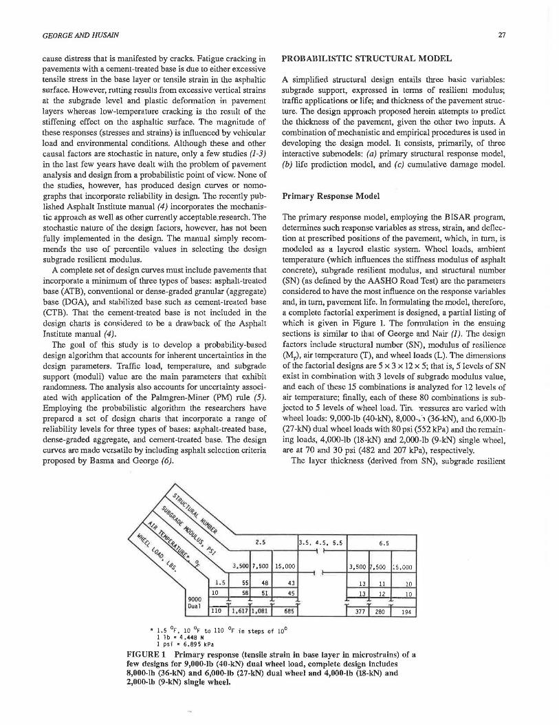
The primary response model, employing the BISAR program, determines such response variables as stress, strain, and deflec­tion at prescribed positions of the pavement, which, in tum, is modeled as a layered elastic system. Wheel loads, ambient temperature (which influences the stiffness modulus of asphalt concrete), subgrade resilient modulus, and structural number (SN) (as defined by the AASHO Road Test) are the parameters considered to have the most influence on the response variables and, in tum, pavement life. In formulating the model, therefore, a complete factorial experiment is designed, a partial listing of which is given in Figure 1. The formulation in the ensuing sections is similar to that of George and Nair (1). The design factors include structural number (SN), modulus of resilience <Mr), air temperature (T), and wheel loads (L). The dimensions of the factorial designs are 5 x 3 x 12 x 5; that is, 5 levels of SN exist in combination with 3 levels of subgrade modulus value, and each of these 15 combinations is analyzed for 12 levels of air temperature; finally, each of these 80 combinations is sub­jected to 5 levels of wheel load. Tirt. iressures are varied with wheel loads: 9,000-lb (40-kN), 8,000-. ·1 (36-kN), and 6,000-lb (27-kN) dual wheel loads with 80 psi (552 kPa) and the remain­ing loads, 4,000-lb (18-kN) and 2,000-lb (9-kN) single wheel, are at 70 and 30 psi (482 and 207 kPa), respectively.

The layer thickness (derived from SN), subgrade resilient

3.5, 4. 5, 5.5 6.5

15 ,000 3,500 ,500 15,000

43 13 11 10 45 10

685 194

* 1.5 °F, 10 °F to 110 °F in steps of 10° 1 1 b • 4 .448 N 1 psi • 6.895 kPa

FIGURE 1 Primary response (tensile strain In base layer in microstralns) or a rew designs for 9,000-lb (40-kN) dual wheel load, complete design includes 8,000-lb (36-kN) and 6,000-lb (27-kN) dual wheel and 4,000-lb (18-kN) and 2,000-lb (9-kN) single wheel.

28

mcxlulus, and wheel loads are direct inputs into the BISAR program. Temperature enters into the analysis as it affects the stress-strain response of bituminous concrete in the surface layer and in the base layer, when applicable. The temperature­rlepemfont morl11li 11re rlerived in two steps 11s describe.d herein. First, the temperatures of both layers in the mcxlel are estimated from the air temperature employing the following empirical relationship (7):

Layer 1

TP = Ta [1 + (3/h1 + 12)] - (102/h1 + 12) + 6

Layer 2

TP =Ta [1 + (3/3h1 +h2 +12)] - (102/3h1 + h2 + 12) + 6

where

TP = pavement temperature; Ta = air temperature; and

h1, h2 = thickness of surface layer, base layer.

(1)

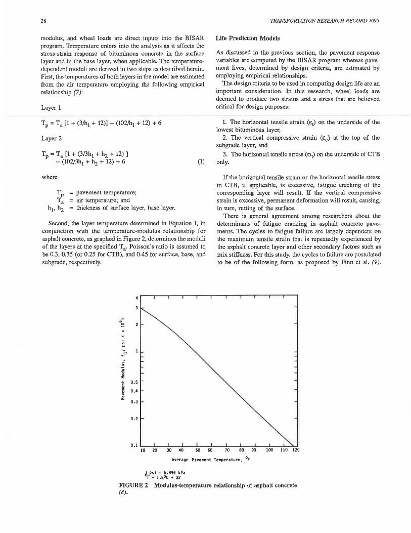
Second, the layer temperature determined in Equation 1, in conjunction with the temperature-modulus relationship for asphalt concrete, as graphed in Figure 2, determines the moduli of the layers at the specified Ta. Poisson's ratio is assumed to be 0.3, 0.35 (or 0.25 for CTB), and 0.45 for surface, base, and subgrade, respectively.

4

3

.., ~ 2

.. 0.

... .; ~ :s

i .. o.s c

i 0.4 > ..

0.. 0.3

0.2

TRANSPORTATION RESEARCH RECORD 1095

Life Prediction Models

As discussed in the previous section, the pavement response variables are computed by the BISAR program whereas pave­ment lives, determined by design criteria, are estimated by employing empirical relationships.

The design criteria to be used in computing design life are an important consideration. In this research, wheel loads are deemed to produce two strains and a stress that are believed critical for design purposes:

1. The horizontal tensile strain (e.) on the underside of the lowest bituminous layer,

2. The vertical compressive strain (Ee) at the top of the subgrade layer, and

3. The horizontal tensile stress (at) on the underside of CTB only.

If the horizontal tensile strain or the horizontal tensile stress in CTH, if applicable, is excessive, fatigue cracking of the corresponding layer will result. If the vertical compressive strain is excessive, permanent deformation will result, causing, in tum, rutting of the surface.

There is general agreement among researchers about the determinants of fatigue cracking in asphalt concrete pave­ments. The cycles to fatigue failure are largely dependent on the maximum tensile strain that is repeatedly experienced by the asphalt concrete layer and other secondary factors such as mix stiffness. For this study, the cycles to failure are postulated to be of the following form, as proposed by Finn et al. (9).

0.1 .... ~--~ ....... ~--~....._~_._~ ..... ~--i~~.._~..._~ ....... ...-.. 10 20 30 40 so 60 70 80 90

Average Pnenent Tet1'4ler1ture, °F

~ psi • 6.894 kPa F = i.eoc + 32

100 110 120

FIGURE 2 Modulus-temperature relationship of asphalt concrete (8).

GEORGE AND HUSAIN

Equation 2 was derived allowing for 45 percent fatigue crack­ing in the wheel paths.

Nr = 18.4(C) x 4.325 x 10-3 (Ett3.29 (IE* I to.854 (2)

where

Nr = number of 18-kip (80-kN) equivalent single axle loads (ESALs) before (fatigue) failure occurs,

Et = tensile strain in asphalt layer (in./in. or mm/ mm),

I E* I = asphalt mixture stiffness modulus (psi or kPa), and

C = function of air voids (V v) and asphalt volume (Vb).

Like the fatigue life equation, the vertical compressive strain criterion is related to number of load applications by an equa­tion of the form

(3)

where Ee is the vertical compressive strain in µ in./in. (µ mm/ mm) at subgrade surface and a, b are fitting coefficients; a = 3.0212 x 1015 and b = 3.571, respectively, as proposed by Brown (10).

A tensile stress criterion for cement-treated base is believed to be relevant and preferred to the tensile strain criterion. This conclusion is reached after an in-depth study of the two criteria and after confirmation that the strain criterion is highly conser­vative in that it predicts significantly shorter life for CTB (11). The fatigue equation that follows is attributable to Scott (12):

crt = 94.4 - 4.71 log Nr (4)

where O't is the initial flexural stress. The life (Nr) of the 900 pavement models is calculated by

employing either Equation 2 or Equation 3 for ATB and DGA pavements and Equation 2, 3, or 4 for CTB pavement. In each case, two or three lives, as applicable, are obtained, one for each critical response value; the smallest of the two or three is used in subsequent calculations. With N f as the dependent variable and L, T, ~. and SN of Table 1 as independent

TABLE 1 DESIGN PARAMETERS

Design Factor

Critical damage (D) Cumulative damage, (d)

Probability Distribution Chart

Log normal Log normal

29

variables, multiple regression models are formulated: for brevity, only one equation for ATB is included here:

Nr = 24144.210 SN-3·803L24.137 1 2·372 exp (0.279SN)

exp (12.600 L - 1128 L2 + 0.041 L3)

exp [1422 (lnT)2

- 0.270 (lnT)3] exp [-2.270 · 10-~

+ 5.048 · 10-13Mi°T2 + 0.037(1~)2] (5)

where

L = wheel load in kips (4.448 kN), T = temperature in degrees Fahrenheit (32 + 1.8°C),

and ~ = subgrade resilient modulus in psi (6.895 kPa).

Cumulative Damage Model

Employing the functional relationship among N f and L, T, ~. and SN and the joint probability density function of random variables L, T, and~ [fL,T,M/l,t,m)], expectation of l/Nr is, by definition,

E[l/NrJ = f f_: f {l/[Nr (L,T,MI'SN)]}

f(L,T,Mr) (l,t,m) dl dt dm (6)

where E [ ] stands for the expected value (mean) of the random variable.

According to the PM rule, if Nr is deterministic, l/Nc repre­sents the "unit damage." Expected value of l/Nr is simply the unit damage induced in a pavement of average structural num­ber by a single load application of mean magnitude at average conditions of temperature and subgrade support.

The most widely used failure criterion of variable-stress fatigue is the Palmgren-Miner hypothesis of linear damage accumulation. As indicated before, both fatigue and rutting are considered to be potential distresses that detract from ser­viceability. For want of a better model, the PM rule is presumed to govern the accumulated rutting damage also. The cumulative damage (~). in accordance with the PM hypothesis, is

Parameters of Probability Dislribution

µD = 1.0; Cn = 0.5 µa = 1.00, 0.80, 0.56 and

(7)

Traffic Air temperature Subgrade modulus

Shifted exponential (Figure 4) Two-parameter Weibull (Figure 5) Log normal

0.40 from Figure 3; Ca= 0.67 A,= 0.45 kip-1, I = 1.0 Characteristic value = 70°F, slope = 3.5 µM = 3,000, 100,000, 20,000, and

r 30,000 psi; CM = 0.2 r

Note: 1 kip= 4,448 kN, 1°F = 1.8°C + 32, and 1 psi= 6.895 kPa.

30

where

~ = cumulative fatigue damage; Il;.jk = the predicted number of applications of

strain range Eijk (stress range crijk> if applicable);

Ne = number of load applications (before failure) of strain range ~jk (stress range crijk• if applicable); and

i, j, and k = discrete values of load (L), temperature (T), and subgrade resilient modulus <1fr), respectively.

Because E or cr, if applicable, is a continuous variable, the expression for damage can be expressed in an integral form. The expected numbe.r of load cycles [n(E)] in the load range(/, I + ~l) applied when the pavement temperature is in the range (t, t + ~t) and subgrade resilient modulus in the interval (m, m + ~) can be expressed as

n(E) = Nf- fL TM (l,t,m) M ~t ~ ' , r

(8)

where N[ is the expected number of mixed traffic load cycles before failure. Assuming probabilistic independence among L, T, and ~. Equation 8 can be rearranged, and, when substituted in Equation 7, an expression for expected cumulative damage (µa) will result:

(9)

It is instructive to rewrite Equation 9 in the following manner:

= Nf- f(SN) E (l/Ne) (10)

where f(SN) is a function of SN. For a given pavement of known structural number, Equation

10 provides for the expected value of cumulative damage as a product of the expected value of damage for a single load cycle, referred to as "unit damage" and the expected number of load applications for failure.

Reliability-Based Design

By using Equation 9, expected cumulative damage (µa) can be solved, provided that the probability density functions of ran­dom variables L, T, and Mr are known. Because of the uncer­tainties in predicting fatigue damage, fatigue life can be esti­mated with only a certain reliability (confidence) level. For example, a fatigue life estimated with a reliability level of 95 percent implies that there is at least a 95 percent chance that the pavement will not show the specified amount of fatigue crack­ing before it reaches its estimated fatigue life.

Before a reliability level can be specified, the probability distribution of /\, needs to he known. Significant experimental evidence has been presented in the literature that indicates that

TRANSPORTATION RESEARCH RECORD 1095

the distribution of fatigue lives at a particular stress level is lognormal (13, 14). If Ne is a random variable lognormally distributed by virture of Equation 7, ~ is also lognormally distributed, ~ = LN(µA, O" a)·

As has been demonstrated experimentally by many inves­tigators, the critical damage at failure (D) is not always close to 1.00 but assumes a wide distribution of values (15). For many materials, this variation appears to follow lognormal distribu­tion, D = LN(µ0 , cr0 ). Because both ~ and D are random variables, reliability (R) can be defined as the event (~ < D). That is,

R = P(~ < D) (11)

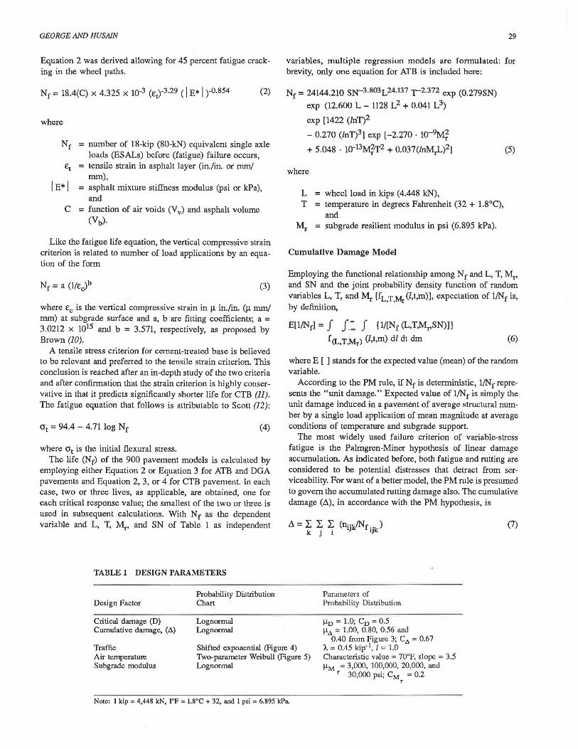
A closed-form expression of µA in terms of Ca and R is given he.rein. Various stops of its derivation can be seen elsewhere (1).

µ~=exp {(1/2) ln(l + C~.) - 0.1116

- cp·1 (R) [ln(l + C3_) + 0.2231]1/2} (12)

where <I> is the standard normal variate. A graphic representation of Equation 12 is shown in Figure

3. Equation 12, in conjunction with Equation 9, renders an explicit solution for the fatigue life (N) of a pavement of given SN; these steps constitute a pavement analysis. Alternatively, a design will entail solving the two equations for SN.

Probability Density Functions for Input Variables

Solving for Equation 9 requires probability distribution func­tions for wheel load, ambient temperature, and subgrade mod-

.s

.4 .. "' ... 0 .. c, . .5 :I

';;; > .3 c, . .8 .. c, . 1.2 ;; i :;:

• i .. ., "' .2

.1...,.,. _________ ~~ 80 90 100

Reliability, percent

FIGURE 3 Maximum allowable µii as a function of R and Ce,; µD = 1, CD= 0.5 (1).

GEORGE AND HUSAIN

ulus. The development of appropriate probability distributions may vary somewhat, depending on availability of data. The authors, however, outline what they believe to be a viable approach.

The wheel load distribution is derived using the Mississippi truck weight data of 1977 and 1980. Passenger cars are excluded from the data. The cumulative truck weight data, along with the "best fit" cumulative distribution function, are shown in Figure 4. A shifted exponential distribution fits the data best with A.= 0.45 kip-1.

The temperature distribution is obtained from the daily tem­perature of a station located in University (northern Mis­sissippi), which is considered to have temperatures representa­tive of the southeastern United States. The 2-year data showed a tendency toward air temperature distributed according to a two-parameter Weibull distribution with characteristic value and slope of distribution of 70°F and 3.5, respectively (Figure 5).

The wide fluctuation of the subgrade moduli, for such rea­sons as temperature or moisture changes or both, must be accounted for by prescribing a probability density function. The subgrade support value data of the AASHO Road Test, when plotted on an annual basis, give rise to a lognormal distribution (1). In view of the direct relationship between subgrade support value and subgrade resilient modulus, a log­normal distribution for the latter may be postulated as well, LN[4500, 900].

Design Charts

When Equation 9 is integrated after the proper substitutions have been made for the probability density functions and N 1 expression as in Equation 5, an expression for µ.1. is obtained for ATB. Similar expressions for DOA and CTB have been obtained; however, they are not reported in this paper. For easy reference, the parameters related to the probability density functions used in those computations are given in Table 1.

"' .. ... .,

1.0

~ 0.8 "' c

c .. &; ,._ L .. ~ 0.4 ... c .. v L .. ...

FL (l) • U-exp(-l[l-1 ]l l<I 1>1

Data

Expclnenthl

o.~....,..-=-~~,,-~~,...........,,...,_~__,....,..~.....,.,.. 1.0 J.O S.O 7.0 9.0 11.0

Wheel Load, kips

1 kip • 4.448 kN

FIGURE 4 Cumulative distribution function of wheel loads, trucks only (shifted exponential with A. = 0.45 klp-1) (1).

0 20 40 60

Tecnperature, °F

°F E i.e0c + 32

80 100 120

FIGURE 5 Relative frequency of temperature data compared with the theoretical distribution (Weibull with scale parameter 70°F and slope 3.5) (1).

31

When an appropriate value of µ.1. has been selected, depending on the desired confidence as in Figure 3, it is a simple pro­cedure to derive and graph explicit relations among the three variables, traffic load repetitions (N[), asphalt concrete thick­ness included in the structural number, and the resilient mod­ulus <Mr). Figures 6 and 7 are illustrative of these charts, for ATB and DOA, respectively. Note that the mixed traffic Nf­needs to be converted into 18-kip (80-kN) ESAL (using AASHO equivalency factors) before the graphs are plotted. A complete set of charts for ATB, DGA, and CTB can be seen in Husain (16). The thickness values shown represent the thick­nesses required to satisfy the tensile strain and compressive strain criteria for ATB and DGA pavement and all three of the criteria for CTB pavement.

EFFECT OF TEMPERATURE ON ASPHALT THICKNESS

Selection of Asphalt Grade for Mix Design

To account for the effect of temperature on asphalt mixture, it is customary to specify softer-grade asphalt in colder climates to reduce low-temperature thermal cracking and harder-grade asphalt in warmer climates to reduce rutting. On the basis of earlier work of Von Quintus et al. (17), Basma and George (6) developed nomographs to help select asphalt grade such that both thermal cracking [not more than 35 ft/1,000 ft2 (115 m/1000 m2)] and rutting [not more than 0.5 in. (12.5 mm)] requirements would be met. Basma and George, employing the nomographs and such weather data as the mean annual air temperature and monthly mean air temperature for some 175 typical stations across the United States, prepared an asphalt selection map identifying five zones commensurate with five grades of asphalt (Figure 8). This map offers a simple pro­cedure for selecting the asphalt grade appropriate to the tem­perature regime of an area. Asphalt selection using this map is in good agreement with that of the Asphalt Institute (4). For

--' cc VI ....

VI :z 0

I­CC u

--' 0.. 0.. cc u .._ !:;: "' I-

SUBGRADE RESILIENT MODULUS, psi x 103

l psi = 6.895 kPa; l kip = 4.448 kN; l inch = 25.4 nm

FIGURE 6 Design chart for asphalt-treated base (80 percent confidence level).

"' 10.

s: _J cc VI .... a. _,. ' ~ .,; l.O :z 0

I-cc ~ --' 0.. o._ cc u .._ .._ ... "' I-

SUBGRADE RESILIENT MODULUS, psi x 103

l psi = 6.895 kPa; l kip = 4.448 kN; l inch • 25.4 11111

FIGURE 7 Design chart for dense-graded aggregate base 8 in. thick (80 percent confidence level).

GEORGE AND HUSAIN

-40 - so -20 -10

C- I

FIGURE 8 Recommended asphalt concrete grades for the United States.

example, the Chicago area with a mean annual air temperature of 50°F (10°C) calls for an asphalt grade of from AC-10 to AC-20 by both methods (Figure 8 and 4, Table VI-1).

AC Thickness Influenced by Asphalt Grade

The question of the effect of asphalt grade on AC thickness now arises. That is, is AC-5 bituminous concrete required for the northern climate as effective (fatigue resistant) as, say, AC-40 mix mandated for the southern climate? To offer an explanation of this dilemma, Basma and George, employing the asphalt selection criteria, prescribed specific asphalt grades for each climatic zone. The "effective moduli" that correspond to various asphalt grades are also reported in the study (Table 2).

Effective modulus is defined as the weighted mean asphalt concrete modulus (weighted with respect to fatigue) (17). Inter­estingly enough, the effective modulus, as given in Table 2, exhibited little variation within a zone, even with the different asphalt grades specified in Figure 8. The data clearly show that

TABLE 2 EFFECTIVE MODULI AND ASPHALT GRADES

Zone

Wet no-freeze Wet freeze and thaw Wet freeze

Ory no-freeze Ory freeze and thaw Dry freeze

psi = 6.895 kPa

Asphalt Grade

AC-40 AC-30 AC-20 AC-10 AC-5 AC-40 AC-30 AC-5 AC-10 AC-30

Effective Modulus

(psi x 105 )

8.40 5.30 4.42 4.43 4.27 4.90 3. 30 2. 50 2. 40 2. 90

33

the prevailing climate of the region stipulates the asphalt grade and therefore determines the asphalt concrete modulus. For example, the effective modulus in a wet no-freeze region may be three times as large as that in a dry freeze region. How this fluctuation affects thickness design is discussed next.

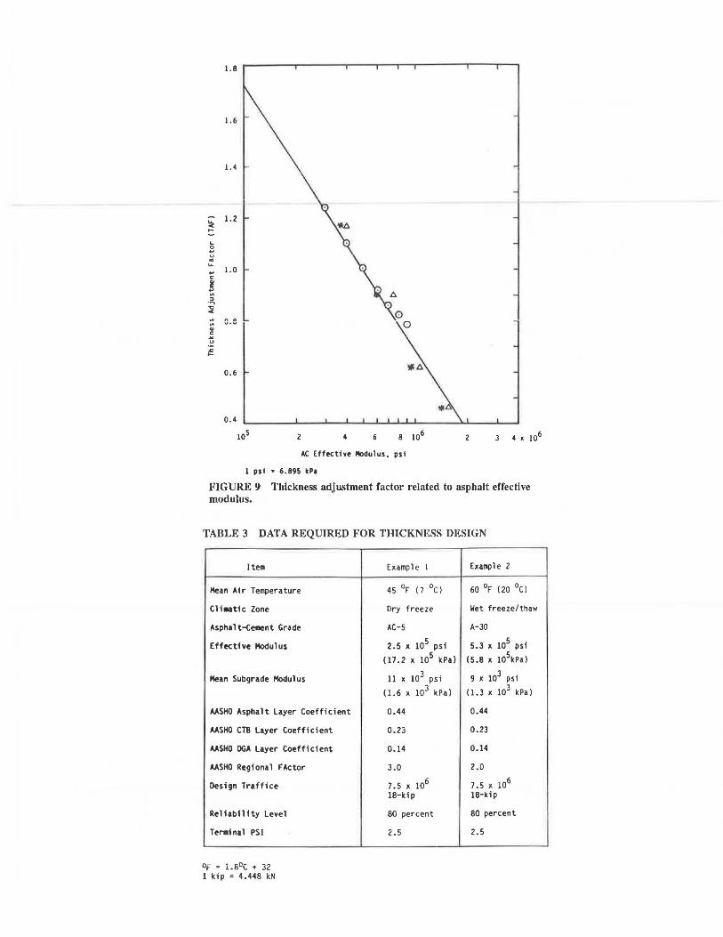
Basma and George studied this problem and defined what is known as modulus factor (MF) (ratio of structural layer coeffi­cient evaluated at the reference modulus of 500,000 psi or 72.S x 103 kPa to that at an arbitrary modulus). Because the layer coefficient and thickness required are related (through struc­tural number), MF could be interpreted as a thickness adjust­ment factor (TAF) that accounts for the modulus fluctuations from region to region. When MF- or TAP-values of this pre­vious study are plotted against the respective moduli, a definite trend is noted in their variations (Figure 9).

Whether or not this relationship is valid is investigated in the present research effort by repeatedly calculating the thickness nomographs, similar to Figures 6 and 7, using a range of effective moduli above and below the reference modulus of 500,000 psi (72.S x la3 kPa). Note that a modulus of 500,000 psi (72.5 x la3 kPa) is used to prepare the nomographs in Figures 6 and 7. The moduli inputs for the calculations are ascertained from temperature distributions (mean and variance) employing Figure 2. For each temperature distribution, two moduli are calculated: a "simple" mean and a "derived" mean (18). The two sets of moduli are subsequently used to calculate asphalt layer thicknesses. Again, the thickness adjustment fac­tors (ratio of thickness of AC for 500,000 psi or 72.S x Hf kPa to that for another modulus) are plotted against the respective moduli. That the TAF -versus-moduli relationship of the present study is in good agreement with that of the previous study attests to the validity of the TAF concept. A trend line compris­ing the two sets of data is shown by a solid line in Figure 9.

The thickness adjustment factor is proposed as a multiplier that would transform the calculated thickness values (from the nomograph) to the "true" design value. Asphalt concrete sur­facing needs to be thicker in regions where the TAF is greater than 1 than it does in regions where the TAF is less than 1. The writers propose that TAF be used as an adjustment factor to account for the modulus variation. That is, when the projected modulus of a region is different from 500,000 psi (72.5 x la3 kPa), the nomographed thickness values should be adjusted employing the TAF. TAF will be greater than 1 when the effective modulus for the region is below the reference value of 500,000 psi and smaller than 1 when the effective modulus is above the reference value. The use of TAF is illustrated in the example problems.

SUMMARY

The design procedure presented in this paper is believed to have successfully incorporated both mechanistic and empirical state-of-the-art information in a viable design methodology. A major improvement in this procedure is the incorporation of structural performance characteristics. Structural performance refers to fatigue cracking and surface rutting. A unique aspect of this design algorithm is that it accounts for variabilities or uncertainties, or both, that are inherent in the design param­eters: traffic load, ambient temperature, and subgrade support

~ .... L 0 ... u .. ... .. c

~ .;:?, .., c ~

~ QI c .. u ~ ....

1.8

1.6

1.4

1.2

1.0

c.e

0.6

0.4

105 4

AC Effecthe llOdul us, psi

l psi • 6.895 kPI

4 • 106

FIGURE 9 Thickness adjustment factor related to asphalt effective modulus.

TABLE 3 DATA REQUIRED FOR THICKNESS DESIGN

Item

Mean Afr Temperature

Cli.atfc Zone

Asphalt-Cement Grade

Effective Modulus

Mean Subgrade Modulus

AASHO Asphalt Layer Coefficient

AASHO CT8 Layer Coefficient

AASHO DGA Layer Coefficient

AASHO Regional FActor

Design Traffice

Reliability Level

Terminal PSI

oF = i.0°c + 32 1 kip = 4.448 kN

Example l Example 2

45 °F ( 7 OC) 60 °F (20 °cl

Dry freeze Wet freeze/thaw

AC-5 A-30

2.5 x 105 psf 5.3 x 105 psi

(17.2 x 105 kPa) (5.8 x l05kPal

11 x 103 psi 9 x 103 psi

(1.6 x 103 kPa) (1.3 x 103 kPa)

0.44 0.44

D.23 0.23

0.14 0.14

3.0 2.0

7.5 x 106 7.5 x 106

18-kip 18-kip

80 percent 80 percent

2.5 2.5

GEORGE AND HUSAIN 35

TABLE 4 COMPARISON WITH OTHER METHODS

Location

Huron, S.D. RF= 3.0 Es= 11,000 psi

Oxford, Miss. RF= 2.0 Es = 9,000 psi

No. of 18-kip ESALs

7.5 x 106

7.5 x 106

Note: 1 psi = 6.895 kPa and 1 in. = 25.4 mm.

conditions. Because the design incorporates reliability in design, the engineer, if he wishes, can exercise a wide range of reliability options commensurate with the functional classifica­tion of the pavement. Design nomographs for two types of base materials, ATB and DGA, are included in this paper; a com­plete set of nomographs for four different reliability levels, however, can be found elsewhere (16).

A rational method for selecting asphalt grade is presented as an integral part of the design procedure. When implementing this criterion for the entire nation, it becomes clear that the desired bituminous mix for each climatic region (six in all) exhibits a unique effective modulus. The region-to-region modulus variation, however, is accounted for by the use of the thickness adjustment factor (multiplying factor) that would transform the nomograph value (of thickness) to the "true" design value.

The example problems presented in the following subsec­tions illustrate the entire procedure, including the use of the thickness adjustment factor. The data required for the thickness design, along with other information for both examples, are given in Table 3.

Example 1: Huron, South Dakota

Enter Figure 6 with design traffic 7.5 x 106 18-kip ESAL and subgrade modulus 11,000 psi (1.6 x lol kPa) and obtain the asphalt layer thickness 11.5 in. (292 mm) for standard condi­tions. Because Figure 6 is prepared by using asphalt modulus 5 x la5 psi (7.25 x HP kPa), the thickness obtained from this figure should be corrected for the asphalt grade, selected for local conditions. From Figure 9, read the TAF = 1.3 corre­sponding to asphall concrete modulus 2.5 x la5 psi (36.3 x lol kPa). Multiply the thickness obtained previously by TAF to get the design asphalt thickness, 1.3 x 11.5 in. = 15.0 in. (381 mm). The design asphalt thickness determined from the present method is compared with thickness obtained from Asphalt Institute (4) and AASHO (19) methods.

Example 2: Oxford, Mississippi

With design traffic 7.5 x 106 18-kip ESAL and subgrade mod­ulus 9 x 103 psi (1.3 x 1a3 kPa), the required thickness of asphalt concrete for standard conditions, from Figure 6, is 12.0

Thickness of Asphalt Concrete (in.) Probabilistic Fatigue Design, 80% Reliability

15.0

11.7

Asphalt Institute (4)

13.3

13.0

AAS HO (19)

9.6

9.3

in. (305 mm). Enter Figure 8 and obtain TAF = 0.97 corre­sponding to 5.30 x 1a5 psi (76.8 x 103 kPa) effective asphalt concrete modulus. Thus the design asphalt concrete thickness is 0.97 x 12.0 in. = 11.7 in. (297 mm).

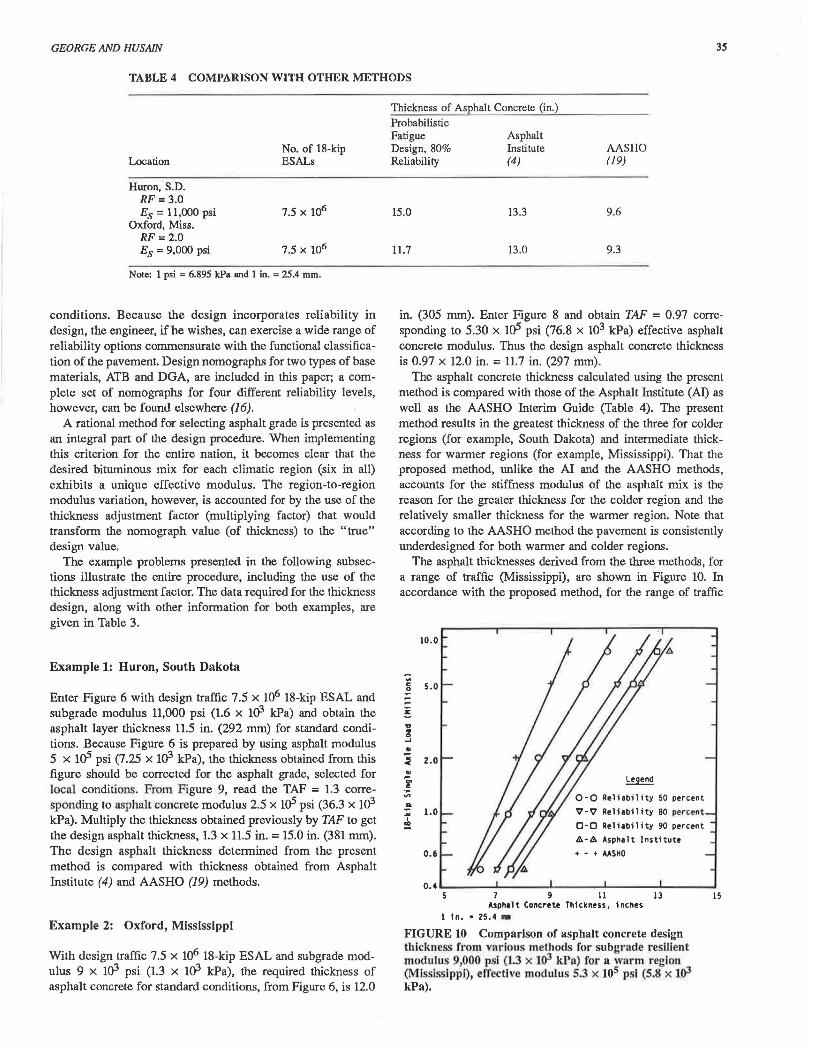
The asphalt concrete thickness calculated using the present method is compared with those of the Asphalt Institute (Al) as well as the AASHO Interim Guide (Table 4). The present method results in the greatest thickness of the three for colder regions (for example, South Dakota) and intermediate thick­ness for warmer regions (for example, Mississippi). That the proposed method, unlike the AI and the AASHO methods, accounts for the stiffness modulus of the asphalt mix is the reason for the greater thickness for the colder region and the relatively smaller thickness for the warmer region. Note that according to the AASHO method the pavement is consistently underdesigned for both warmer and colder regions.

The asphalt thicknesses derived from the three methods, for a range of traffic (Mississippi), are shown in Figure 10. In accordance with the proposed method, for the range of traffic

10.0

.. g 5.0

;: i ,, :!l _, .. ~ 2.0 .. "' c

... ... I

~

1.0

0.6

Legend

0-0 Reliability 50 percent

V-V Reliability BO percent

0-0 Reliability 90 percent

//:i.-A Asphalt Institute

+ - + AASHO

0.4...._~~~.._~~--' ..... ~~-"'~~~--I.~~~.-. s 7 9 11 13

Asph1l t Concrete Th1 ckness, inches 1 in. • 25.4 •

FIGURE 10 Comparison of asphalt concrete design thickness from various methods for subgrade reslUent modulus 9,000 psi (l.3 x 1a3 kPa) for a warm region (Mississippi), effectlve modulus 5.3 x 105 psi (5.8 x 1a3 kPa).

15

36

levels considered and for all three of the reliability levels, the required thicknesses lie between those required by AI and AASHO methods.

These examples reaffirm the conclusion that the proposed design procedure is sound with respect to the use of mechanis­cic merhods, probabilisric considerarion of variables, and, finally, asphalt grade selection.

ACKNOWLEDGMENTS

This paper is a part of the study titled "Overlay Design and Reflection Cracking Study for Flexible Pavements," sponsored by the Mississippi Highway Department and the U.S. Depart­ment of Transportation, Federal Highway Administration. The authors wish to acknowledge the Shell-Laboratorium for their permission to use the BlSAR program.

REFERENCES

1. K. P. George and S. K. Nair. Probabilistic Fatigue Design for Aexible Pavements. Proc., Fifth International Conference on the Structural Design of Asphalt Pavements, The Netherlands, 1982.

2. W. J. Kenis. Predictive Design Procedures-A Design Method for Aexible Pavements Using the VESYS Structural Subsystem. Proc., Fourth International Conference on the Structural Design of Asphalt Pavements, The University of Michigan, Ann Arbor, 1977.

3. R. B. Kulkarni. Probabilistic Prediction of Pavement Distress Models. Proc., Third International Conference on Applications of Statistics and Probability in Soil and Structural Engineering, Sydney, Australia, 1979.

4. Thickness Design-Asphalt Pavements for Highways and Streets. MS-1. The Asphalt Institute, College Park, Md., 1981.

5. M.A. Miner. Cumulative Damage in Fatigue. Transactions of the ASME, Vol. 67, 1945.

6. A. A. Basma and K. P. George. Environmental Factors in Aexible Pavement Design. In Transportation Research Record 954, TRB, National Research Council, Washington, D.C,, 1984, pp. 52-58.

7. D. Hwang and M. W. Witezak. Program DAMA: User's Manual. University of Maryland, College Park, 1979.

8. K. Majidzadeh and J. Ilves. Flexible Pavement Overlay Design.

TRANSPORTATION RESEARCH RECORD 1095

Report GHWA/RD-81/032. Federal Highway Administration, Vol. 1., 1981.

9. F. N. Finn, C. Saraf, R. Kulkarni, K. Nair, W. Smith, and A. Abdullah. The Use of Distress Prediction Subsystems for the Design of Pavement Structure. Proc., Fourth International Con­ference on the Structural Design of Asphalt Pavements, The Uni­versity of Michigan, Ann Arbor, 1977.

10. S. F. Brown, J. M. Brunton, and P. S. Pell. The Development and Implementation of Analytical Pavement Design for British Condi­tions. Proc., Fifth International Conference on the Structural Design of Asphalt Pavements, Delft University, Delft, The Nether­lands, 1982, pp. 3-16.

11. K. P. George. Material Parameters for Pavement Design Using AASHO Interim Guide. Final Report. The University of Mis­sissippi, University, 1981.

12. J. L. M. Scott. Flexural Stress-Strain Characteristics of Saskatchewan Soil-Cement Technical Report 23. Saskatchewan Department of Highway, Saskatoon, 1974.

13. P. S. Pell and I. F. Taylor. Asphaltic Road Materials in Fatigue. Proc., Association of Asphalt Paving Technologists, Vol. 38, 1969.

14. C. L. Monismith et al. Asphalt Mixture Behavior in Repeated Flexure. Report 705. Institute of Transportation and Traffic Engi­neering, University of California, Irvine, 1972.

15. P. H. Wirsching and J. T. P. Yao. A Probabilistic Design Approach Using the Palmgren-Miner Hypothesis. Proc., Nation~/ St~uctural Engineering Conference, ASCE, Vol. 1, 1976.

16. S. Husain. Evaluation of Flexible Pavement and Overlay Design. Ph.D. dissertation. The University of Mississippi, University, 1985.

17. H. L. Von Quintus, F. N. Finn, W. R. Hudson, and F. L. Roberts. Flexible and Composite Structures for Premium Pavements, Vol. 2: Design Manual. FHWAH-RD-80. FHWA, U.S. Department of Transportation, 1980.

18. J. R. Benjamin and C. A. Cornell. Probability Statistics and Deci­sion for Civil Engineer. McGraw-Hill Book Company, New York, 1970.

19. AASHO Interim Guide 1972. AASHO, Washington, D.C., 1972.

Publication of this paper sponsored by Committee on Flexible Pave­ments.

The opinions, findings~ and conclusions e~r.pressed in this paper are those of the authors and not necessarily those of the Mississippi Stale Highway Department or the Federal Highway Administration. This paper does not constitute a standard, specification, or regulation.