Performance Enhancements for the Lattice-Boltzmann Solver in the LAVA

Framework

Michael Barad, Joseph Kocheemoolayil, Gerrit Stich, and Cetin Kiris

Computational Aerosciences BranchNASA Ames Research Center

ICCFD10 2018July 9-13, Barcelona, Spain

ICCFD10-2018-101

ü Increase predictive use of computational aerosciences capabilities for next generation aviation and space vehicle concepts.• The next frontier is to use wall modeled and/or wall resolved large-eddy simulation

(LES) to predict:

Motivation

2

Unsteady loads and fatigue

Buffet and shock BL interaction

Fan, jet, and airframe noise

Active flow control

ü Need novel techniques for reducing the computational resources consumed by current high-fidelity CAA• Need routine acoustic analysis of aircraft components at full-scale Reynolds number from

first principles• Need an order of magnitude or more reduction in wall time to solution!

Contra-Rotating Open Rotor PropulsionLanding Gear Acoustics

Launch Abort System Analysis for OrionLow Density Supersonic Decelerators

Launch Pad Design

Many successful applications of High-Performance High-Fidelity Cartesian methods to NASA Mission critical applications

SOFIA Airplane Cavity Acoustics

ISS Battery Analysis

Unsteady Rocket Loads

ü Computational Requirements• Space-time resolution requirements for acoustics problems are demanding. • Resources used for recent Cartesian Navier-Stokes simulations:

• Launch Environment: ~200 million cells, ~7 days (1000 cores)• Parachute: 200 million cells, 3 days (2000 cores)• Contra-Rotating Open Rotor: 360 million cells, 14 days (1400 cores)• Launch Abort System: 400 million cells, 28 days (2000 cores)• Landing Gear: 298 million cells, 20 days (3000 cores)

Challenges in Computational Aero-Acoustics

4

ü Physics:• Governs space time evolution of Density Distribution Functions• Equilibrium distribution functions are truncated Maxwell-Boltzmann distributions• Relaxation time related to kinematic viscosity• Pressure related to density through the isothermal ideal gas law• Lattice Boltzmann Equations (LBE) recover the Navier-Stokes equations in the

low Mach number limit

ü Numerics:• Extremely efficient ‘collide at nodes and stream along links’ discrete analog to the

Boltzmann equation • Particles bound to a regularly spaced lattice collide at nodes relaxing towards the

local equilibrium (RHS)

• Post-collision distribution functions hop on to neighboring nodes along the lattice links (LHS) – Exact, dissipation-free advection from simple ‘copy’ operation

• Macroscopic quantities such as density and momentum are moments of the density distribution functions in the discrete velocity space

Lattice-Boltzmann Method (LBM)

5

ü LBM Benefits: • Ultra high performance: excellent data locality, vectorizable, scalable.• Minimal numerical dissipation that is critical for computational aeroacoustics, and ideal for Large

Eddy Simulations.• Simulation of arbitrarily complex geometry with high performance structured adaptive mesh

refinement is straight forward, bypassing manual and/or expensive meshing bottlenecks.

ü NASA’s LAVA-LBM • Progress to Date:

• LAVA Cartesian infrastructure has been re-factored into Navier-Stokes (NS) and LBM. Existing LAVA Cartesian data structures and algorithms are utilized.

• Parallel Structured Adaptive Mesh Refinement (SAMR) meshing, robust collision models, second-order boundary conditions, all implemented.

• Verification & validation: Taylor-Green vortex, flow past a cylinder, and nose landing gear.• A 12 to 15 times speedup compared to LAVA-Cart-NS was demonstrated for landing gear.

• Current Efforts:• Performance

• Enhanced Accuracy at Coarse/Fine interface• Parallel Efficiency and Scaling

• Moving Geometry• Wall Modeling• High Mach formulation

Lattice-Boltzmann Method (LBM)

6

Focus on these for this paper

In testing phase

Initial stages of development

Recent LAVA-LBM Success for Landing Gear:

LBM @ 1.6 billion – Velocity Magnitude at Centerline 102 103 104

Frequency (Hz)

10�14

10�13

10�12

10�11

10�10

10�9

10�8

10�7

10�6

10�5

10�4

PSD

(psi

2 /H

z)

Channel 5

LB: 90 MillionLB: 260 MillionLB: 1.6 BillionEXP-UFAFF

Surface Pressure Spectra at Sensor Locations

9

Near Field Noise Predictions

“Lattice Boltzmann and Navier-Stokes Cartesian CFD Approaches for Airframe Noise Predictions”, Barad, Kocheemoolayil, Kiris, AIAA 2017-4404

7

Lessons from LAVA LBM Landing Gear Simulations

LBM @ 1.6 billion – Velocity Magnitude at Centerline

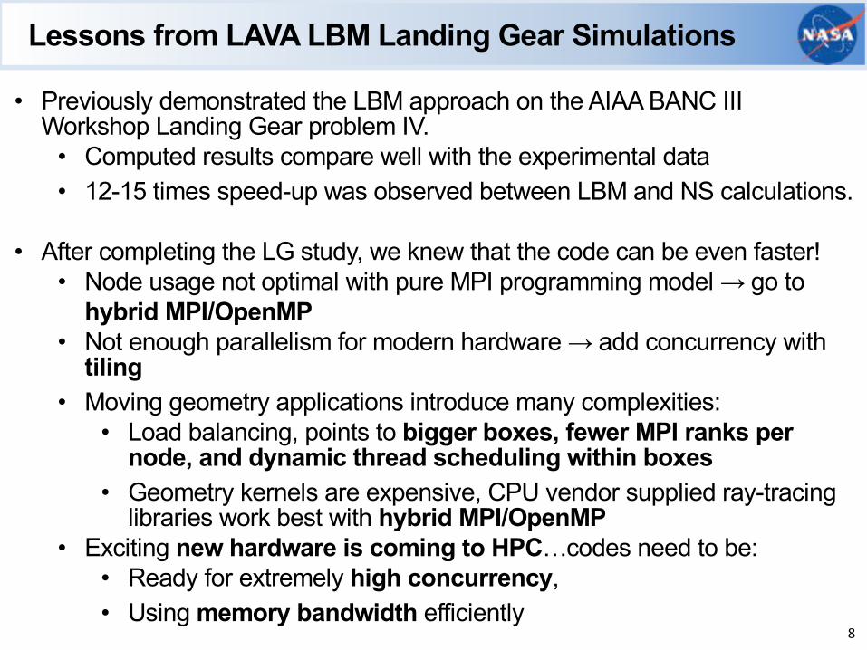
• Previously demonstrated the LBM approach on the AIAA BANC III Workshop Landing Gear problem IV.

• Computed results compare well with the experimental data• 12-15 times speed-up was observed between LBM and NS calculations.

• After completing the LG study, we knew that the code can be even faster!• Node usage not optimal with pure MPI programming model → go to

hybrid MPI/OpenMP• Not enough parallelism for modern hardware → add concurrency with

tiling• Moving geometry applications introduce many complexities:

• Load balancing, points to bigger boxes, fewer MPI ranks per node, and dynamic thread scheduling within boxes

• Geometry kernels are expensive, CPU vendor supplied ray-tracing libraries work best with hybrid MPI/OpenMP

• Exciting new hardware is coming to HPC…codes need to be: • Ready for extremely high concurrency, • Using memory bandwidth efficiently

8

Conservative Coarse/Fine Interface

Sketch of conservative recursive sub-cycling algorithm. • Block structured AMR showing 3 levels of refinement by factor 2. • Arrows indicate direction of information propagation:

• streaming (blue), • coarse-to-fine communication (red), • fine-to-coarse communication (green).

Refs: Schornbaum and Rude 2016, Rohde et al 2006, Chen et al 2006. 9

Conservative Coarse/Fine Interface2D Conservation Test:

10

Conservative Coarse/Fine Interface

11

3D Conservation Test:

More Parallelism: Tiling (a) Regular Tiles (b) Pencil Tiles

Different tile types for a single box: (a) regular tiles (8D), including inner (blue) and outer (red); and (b) pencil tiles (green) for contiguous memory accesses

The box shown has 64D cells, plus 3 ghost layers. 3D tiles are conceptually similar.

12

More Parallelism: Tiling + OpenMPAdding another level of parallelism has many benefits:

• Loop collapse: OpenMP over boxes on a proc & tiles in each box #pragma omp for schedule(dynamic) collapse(2)

for (int ibox = 0; ibox < nbox; ++ibox)

{for (int itile = 0;itile < ntile; ++itile)

{

work(ibox,itile);

}

}

• Improved load balancing for irregularities: • Complex geometry• AMR

• Bigger boxes are possible which improves surface/volume ratios and reduces MPI expense

• Asynchronous communication is enabled:• Outer tiles are computed first, then non-blocking MPI sends• Inner tiles then computed• Finish MPI comms

13

LAVA LBM: Verification and ValidationTURBULENT TAYLOR GREEN VORTEX BREAKDOWN TEST CASE:• Motivation:

• Simple low speed workshop case for testing high-order solvers

• Illustrates ability of solver to simulate turbulent energy cascade

• Periodic boundary conditions• Setup:

• Analytic initial condition• Mach = 0.1• Reynolds Number = 1600

• Triply periodic flow in a box• Comparisons:

• LAVA’s Lattice Boltzmann (LB) solver captures the turbulent kinetic energy cascade from large scales to small scales extremely well.

• Performance compared to LAVA’s Cartesian grid Navier-Stokes WENO solver showed a factor of 50 speedup.

0

0.2

0.4

0.6

0.8

1

0 5 10 15 20

E(t)/

E(0)

t

Lattice Boltzmann (1283)Navier-Stokes (1283)

Reference (5123)

Ta ylo r G reen kinetic energy d eca y using LA VA So lve rs

Ta ylo r G reen vortic ity b rea kd ow n. Im a ge c red it: 3rd In te rna tiona l W orkshop on H igh-O rd er C FD M ethod s (Beck et a l)

CFD

14

TGV Profiling: SetupTaylor-Green Vortex (TGV) test case:

• 2563 cells per node problem size, unless noted otherwise • Single static level (i.e. no AMR issues)• No geometry• 64 time-steps performed, time to solution measured• All simulations conducted on Skylake nodes on NASA’s Pleiades

supercomputer (1 node has 2 sockets, 20 physical cores per socket)

• Focused on 3 versions of the code:• Baseline (no tiling)• Tiling with data copies to tiles• Tiling without data copies to tiles

15

See paper for these results

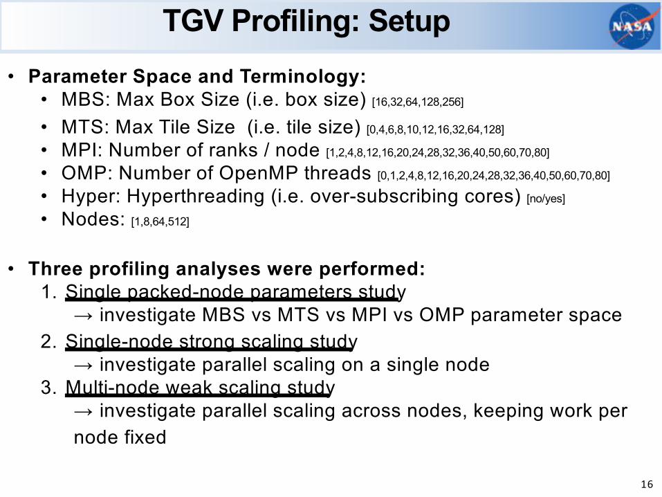
TGV Profiling: Setup• Parameter Space and Terminology:

• MBS: Max Box Size (i.e. box size) [16,32,64,128,256]

• MTS: Max Tile Size (i.e. tile size) [0,4,6,8,10,12,16,32,64,128]

• MPI: Number of ranks / node [1,2,4,8,12,16,20,24,28,32,36,40,50,60,70,80]

• OMP: Number of OpenMP threads [0,1,2,4,8,12,16,20,24,28,32,36,40,50,60,70,80]

• Hyper: Hyperthreading (i.e. over-subscribing cores) [no/yes]

• Nodes: [1,8,64,512]

• Three profiling analyses were performed:1. Single packed-node parameters study

→ investigate MBS vs MTS vs MPI vs OMP parameter space2. Single-node strong scaling study

→ investigate parallel scaling on a single node3. Multi-node weak scaling study

→ investigate parallel scaling across nodes, keeping work per node fixed

16

TGV Profiling: Single Packed-Node

20 40 60 80 100 120Box Size

102

Tim

e[s

]

40 MPI, 0 OMP, 0 MTS, Min = 57.13 80 MPI, 0 OMP, 0 MTS, Min = 66.55; Hyper

Baseline (no tiling), sensitivity to box size (MBS):

17

TGV Profiling: Single Packed-Node

20 40 60 80 100 120Box Size

102

Tim

e[s

]

40 MPI, 0 OMP, 0 MTS, Min = 48.3740 MPI, 0 OMP, 4 MTS, Min = 37.8740 MPI, 0 OMP, 6 MTS, Min = 39.2240 MPI, 0 OMP, 8 MTS, Min = 36.7340 MPI, 0 OMP, 10 MTS, Min = 36.7440 MPI, 0 OMP, 12 MTS, Min = 37.8440 MPI, 0 OMP, 16 MTS, Min = 38.9240 MPI, 0 OMP, 32 MTS, Min = 36.992 MPI, 20 OMP, 4 MTS, Min = 34.942 MPI, 20 OMP, 6 MTS, Min = 34.15

2 MPI, 20 OMP, 8 MTS, Min = 32.182 MPI, 20 OMP, 10 MTS, Min = 31.872 MPI, 20 OMP, 12 MTS, Min = 28.702 MPI, 20 OMP, 16 MTS, Min = 30.292 MPI, 20 OMP, 32 MTS, Min = 29.6880 MPI, 0 OMP, 0 MTS, Min = 79.74; Hyper80 MPI, 0 OMP, 4 MTS, Min = 46.37; Hyper80 MPI, 0 OMP, 6 MTS, Min = 49.67; Hyper80 MPI, 0 OMP, 8 MTS, Min = 44.64; Hyper80 MPI, 0 OMP, 10 MTS, Min = 51.65; Hyper

80 MPI, 0 OMP, 12 MTS, Min = 53.96; Hyper80 MPI, 0 OMP, 16 MTS, Min = 52.10; Hyper80 MPI, 0 OMP, 32 MTS, Min = 51.19; Hyper2 MPI, 40 OMP, 4 MTS, Min = 30.25; Hyper2 MPI, 40 OMP, 6 MTS, Min = 27.38; Hyper2 MPI, 40 OMP, 8 MTS, Min = 28.98; Hyper2 MPI, 40 OMP, 10 MTS, Min = 28.17; Hyper2 MPI, 40 OMP, 12 MTS, Min = 24.84; Hyper2 MPI, 40 OMP, 16 MTS, Min = 24.92; Hyper2 MPI, 40 OMP, 32 MTS, Min = 25.77; Hyper

Optimized, without copy into tiles, sensitivity to box size (MBS):

18

Conclusion: bigger boxes are better, andwithout copy is better2 MPI/node, 40 OMP/MPI, 12 MTS

TGV Profiling: Single Packed-NodeOptimized, without copy into tiles, sensitivity to tile size (MTS):

0 5 10 15 20 25 30Tile Size

102

Tim

e[s

]

40 MPI, 0 OMP, 16 MBS, Min = 88.7940 MPI, 0 OMP, 32 MBS, Min = 49.1340 MPI, 0 OMP, 64 MBS, Min = 36.732 MPI, 20 OMP, 16 MBS, Min = 96.982 MPI, 20 OMP, 32 MBS, Min = 52.81

2 MPI, 20 OMP, 64 MBS, Min = 35.132 MPI, 20 OMP, 128 MBS, Min = 28.7080 MPI, 0 OMP, 16 MBS, Min = 80.69; Hyper80 MPI, 0 OMP, 32 MBS, Min = 44.64; Hyper

2 MPI, 40 OMP, 16 MBS, Min = 87.04; Hyper2 MPI, 40 OMP, 32 MBS, Min = 45.46; Hyper2 MPI, 40 OMP, 64 MBS, Min = 30.14; Hyper2 MPI, 40 OMP, 128 MBS, Min = 24.84; Hyper

19

Conclusion: without copy code is less sensitive to tile size, and much better than with copy

TGV Profiling: Single-Node Strong ScalingOptimized, without copy into tiles: Hyperthreading

region is marked with gray shading

Conclusion: 2 MPI per node (i.e. 1 per socket) has best performance

20

TGV Profiling: Multi-Node Weak Scaling

101 102 103 104

Millions of Cells

20

40

60

80

100

120

140

Tim

e[s

]

0 OMP, 16 MBS, 0 MTS0 OMP, 32 MBS, 0 MTS

0 OMP, 64 MBS, 0 MTS0 OMP, 16 MBS, 0 MTS; Hyper

0 OMP, 32 MBS, 0 MTS; Hyper

Baseline (no tiling):

21

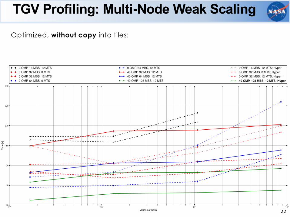
TGV Profiling: Multi-Node Weak ScalingOptimized, without copy into tiles:

101 102 103 104

Millions of Cells

20

40

60

80

100

120

140

Tim

e[s

]

0 OMP, 16 MBS, 12 MTS0 OMP, 32 MBS, 0 MTS0 OMP, 32 MBS, 12 MTS0 OMP, 64 MBS, 0 MTS

0 OMP, 64 MBS, 12 MTS40 OMP, 32 MBS, 12 MTS40 OMP, 64 MBS, 12 MTS40 OMP, 128 MBS, 12 MTS

0 OMP, 16 MBS, 12 MTS; Hyper0 OMP, 32 MBS, 0 MTS; Hyper0 OMP, 32 MBS, 12 MTS; Hyper40 OMP, 128 MBS, 12 MTS; Hyper

22

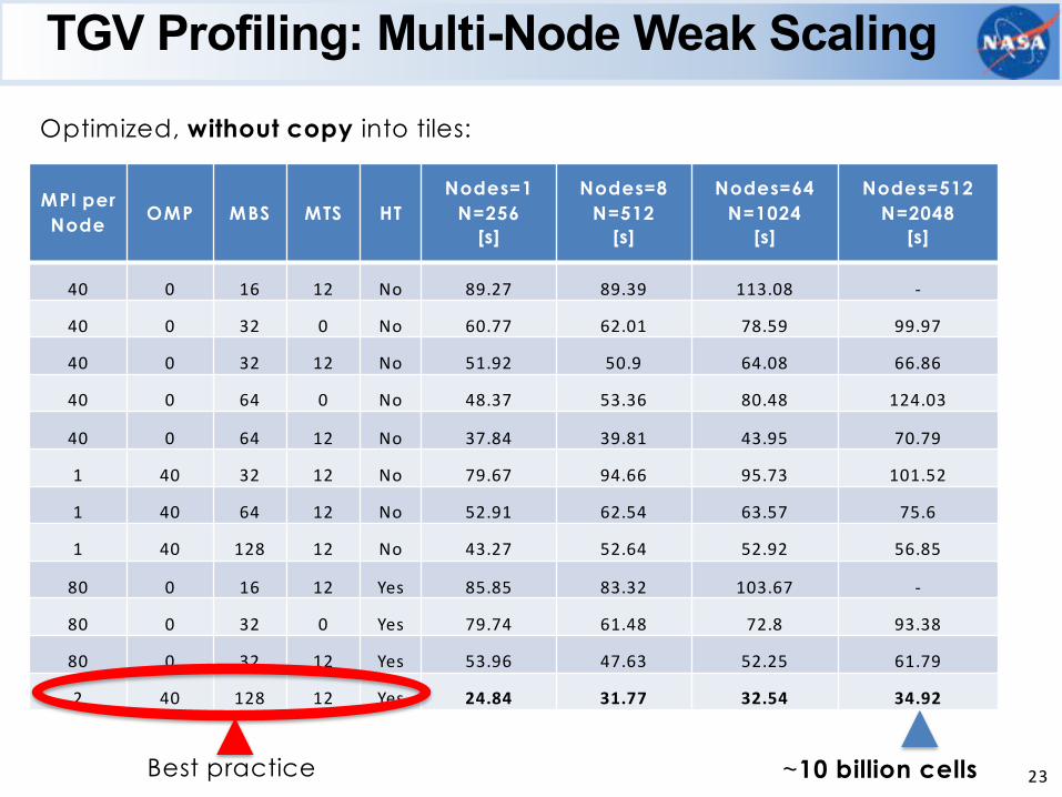
TGV Profiling: Multi-Node Weak Scaling

~10 billion cells 23

Optimized, without copy into tiles:

MPI perNode OMP MBS MTS HT

Nodes=1N=256

[s]

Nodes=8N=512

[s]

Nodes=64N=1024

[s]

Nodes=512N=2048

[s]

40 0 16 12 No 89.27 89.39 113.08 -

40 0 32 0 No 60.77 62.01 78.59 99.97

40 0 32 12 No 51.92 50.9 64.08 66.86

40 0 64 0 No 48.37 53.36 80.48 124.03

40 0 64 12 No 37.84 39.81 43.95 70.79

1 40 32 12 No 79.67 94.66 95.73 101.52

1 40 64 12 No 52.91 62.54 63.57 75.6

1 40 128 12 No 43.27 52.64 52.92 56.85

80 0 16 12 Yes 85.85 83.32 103.67 -

80 0 32 0 Yes 79.74 61.48 72.8 93.38

80 0 32 12 Yes 53.96 47.63 52.25 61.79

2 40 128 12 Yes 24.84 31.77 32.54 34.92

Best practice

Bonus: GPU Hackathon 2018The LAVA team participated in a “GPU Hackathon” in Boulder, CO (06/2018)Focused on a highly simplified LBM-mini app (single level TGV)

25631963

1283

963

643

Skylake Node CPU

2563

Nvidia V100 GPU

Hackathon

optimizations

?

Strong scaling with varying problem size:

Mill

ion

s o

f C

ells

Up

da

ted

pe

r Se

co

nd

24

Remaining Challenges for LAVA-LBM-GPU

The following key operations are implemented efficiently on the CPU, but not yet addressed during the hackathon for GPU:• MPI parallel

• AMR operators

• Immersed boundaries• Fixed geometry

• Introduces load imbalances at both simulation startup and during time-stepping

• Treated using structured looping in LAVA -> should map to GPU with some effort

• Moving geometry• Major cost / load imbalances are introduced at every

timestep (re-computing geometry intersections, etc).• Expense on CPU treated using highly optimized vendor

supplied ray-tracing kernels (Embree). Enabling technology for CPU calcs.

• On CPU this is currently roughly a 1.2-1.5x hit in performance, not sure how this will be addressed on the GPU. Try using NVIDIA OptiX.

25

LAVA-NS-CPU

LAVA-LBM-CPU

TGV Profiling: SummaryFor the simple Taylor-Green Vortex problem:

• Found that copying into small tile sized memory is slower than just using the box based memory layout. Not enough re-use in LBM for cache-blocking.

• Developed best practices:• Larger boxes are better• Tile sizes of 8-12 are superior than smaller or larger• Hyperthreading yields a small improvement (~1.16x speedup)• 1 MPI per socket, 40 OMP threads per socket (i.e. hyperthreaded)

• Achieved a 2.3x speedup over the baseline code for a single Skylake-SP CPU node containing 40 physical cores,

• Achieved a 2.14x speedup over the baseline code for 64 Skylake-SP nodes containing 2560 cores

• Scaled the code almost perfectly to 20480 physical cores where the problem size was ~10 billion cells

• LAVA-LBM-GPU mini-app on Nvidia V100 yielded 11.5x speedup vs CPU baseline. Could result in O(100)x speedup for full-app vs LAVA-NS-CPU. 26

Next Steps• Further code optimizations for:

• Moving geometry and • Adaptive meshing

• Improve wall modeling for arbitrarily complex geometry at high Reynolds numbers• Extend Mach number range to transonic and high speed flows

LAVA LBM full aircraft (in progress)

HLPW3, JSM, Case 2c, ! = 20.59°

27

28

Acknowledgments

• This work was partially supported by the NASA ARMD’s Transformational Tools and Technologies (TTT) project and Revolutionary Computational Aerosciences (RCA) sub-project.

• LAVA team members in the Computational Aerosciences Branch at NASA Ames Research Center for many fruitful discussions

• Computer time provided by NASA Advanced Supercomputing (NAS) facility at NASA Ames Research Center

Questions ?

29