post-newtonian and post-minkowskian approximations

Post-Newtonian and Post-MinkowskianApproximations

Alexandre Le Tiec

Laboratoire Univers et TheoriesObservatoire de Paris / CNRS

Gravity@Malta 2018 Alexandre Le Tiec

Modelling coalescing compact binaries

numerical relativity

postNewtonian theory

log10

(m2 /m

1)

0 1 2 3

0

1

2

3

4

4

log10

(r /m)

perturbation theory & selfforce

(com

pact

ness

)

mass ratio

−1





log10

(m2 /m

1)

0 1 2 3

0

1

2

3

4

4

log10

(r /m)


(com

pact

ness

)

mass ratio

−1 m1

m2


B. Wardell’s talk




log10

(m2 /m

1)

0 1 2 3

0

1

2

3

4

4

log10

(r /m)


(com

pact

ness

)

mass ratio

−1

m1

m2


See talks by:

• P. Schmidt

• U. Sperhake




log10

(m2 /m

1)

0 1 2 3

0

1

2

3

4

4

log10

(r /m)


(com

pact

ness

)

mass ratio

−1m

1

m2

r


v2

c2∼ Gm

c2r 1




log10

(m2 /m

1)

0 1 2 3

0

1

2

3

4

4

log10

(r /m)


(com

pact

ness

)

mass ratio

−1m

1

m2

r


v2

c2∼ Gm

c2r 1

See talks by:

• M. Haney

• Y. Boetzel

• N. Tenorio Maia

• Z. Keresztes

Small parameter

ε ∼ v212

c2∼ Gm

r12c2 1 m

2

m1

r12

v2

v1

Example

g00(t, x) = −1 +2Gm1

r1c2︸︷︷︸Newtonian

+4Gm2v2

2

r2c4︸︷︷︸1PN term

+ · · ·+ (1↔ 2)

Notation

nPN order refers to effects O(c−2n) with respect to “Newtonian” solution


Small parameter

ε ∼ v212

c2∼ Gm

r12c2 1 m

2

m1

x

r1

r2

r12

v2

v1

Example

g00(t, x) = −1 +2Gm1

r1c2︸︷︷︸Newtonian

+4Gm2v2

2

r2c4︸︷︷︸1PN term

+ · · ·+ (1↔ 2)

Notation

nPN order refers to effects O(c−2n) with respect to “Newtonian” solution


A wave generation formalism

t

near zone

wave zone

diagram not to scale

r < d R

R λGW

r λGWd

exterior region

λGW


(Figure credit: Buonanno & Sathyaprakash 2015)

Two-body equations of motion

m1

m2

r

v2

v1

GW

GW

n

dv1

dt= −Gm2

r2n +

A1PN

c2+A2PN

c4︸︷︷︸conservative terms

+A2.5PN

c5︸︷︷︸rad. reac.

+A3PN

c6︸︷︷︸cons. term

+A3.5PN


+ · · ·


State of the art: 4PN equations of motion

dv1

dt= −Gm2

r2n +

A1PN

c2+A2PN

c4︸︷︷︸conservative terms

+A2.5PN


+A3PN

c6︸︷︷︸cons. term

+A3.5PN


+A4PN

c8︸︷︷︸cons. term+ rad. tail

+ · · ·

3PN

[Jaranowski & Schafer 1999; Damour, Jaranowski & Schafer 2001] ADM Hamiltonian

[Blanchet & Faye 2001; de Andrade, Blanchet & Faye 2001] Harmonic EOM

[Itoh & Futamase 2003; Itoh 2004] Surface integral

[Foffa & Sturani 2011] Effective field theory

4PN

[Jaranowski & Schafer 2012, 2013; Damour, Jaranowski & Schafer 2014] ADM Hamiltonian

[Bernard, Blanchet, Bohe, Faye, Marchant & Marsat 2015, 2016, 2017] Fokker Lagrangian

[Foffa, Mastrolia, Sturani & Sturm 2012, 2013, 2017] (partial results) Effective field theory


Gravitational-wave tail effect at 4PN order[Blanchet & Damour 1988, Foffa & Sturani 2013, Galley et al. 2016]

• Starting at 4PN order, the near-zone metric depends onthe entire past history of the source:

g tail00 (t, x) = −8G 2M

5c10x ix j

∫ t

−∞dt ′Q

(7)ij (t ′) ln

(c(t − t ′)

2r

)

• This leads to a 4PN non-local-in-timecontribution to the Fokker action:

S tailF =

G 2M

5c8

∫ ∫dt dt ′

|t − t ′|Q(3)ij (t)Q

(3)ij (t ′)

• And to a 1.5PN relative correction tothe leading radiation-reaction force


Phasing for inspiralling compact binaries

• Conservative orbital dynamics → 4PN binding energy

E (ω) = −µ2

(mω)2/3︸︷︷︸Newtonian

binding energy

(1 + · · ·

)︸︷︷︸4PN relative

correction

• Wave generation formalism → 3.5PN GW energy flux

F(ω) =32

5ν2 (mω)5︸︷︷︸

Einstein’squad. formula

(1 + · · ·

)︸︷︷︸

3.5PN relativecorrection

• Energy balance → 3.5PN orbital phase and GW phase

dE

dt= −F

=⇒ dω

dt= −F(ω)

E ′(ω)=⇒ φ(t) =

∫ t

ω(t ′)dt ′




E (ω) = −µ2


binding energy

(1 + · · ·


correction


F(ω) =32

5ν2 (mω)5︸︷︷︸


(1 + · · ·

)︸︷︷︸



dE

dt= −F =⇒ dω

dt= −F(ω)

E ′(ω)

=⇒ φ(t) =

∫ t

ω(t ′)dt ′




E (ω) = −µ2


binding energy

(1 + · · ·


correction


F(ω) =32

5ν2 (mω)5︸︷︷︸


(1 + · · ·

)︸︷︷︸



dE

dt= −F =⇒ dω

dt= −F(ω)

E ′(ω)=⇒ φ(t) =

∫ t

ω(t ′) dt ′


Measurement of PN parameters


[LIGO/Virgo 2016]

Spins of supermassive black holes[Reynolds 2013]

χ

M (106 M)


Binary systems of spinning compact bodies


(Figure credit: L. Blanchet)

Spin-orbit coupling at leading order[Barker & O’Connell 1975]

dSa

dt= Ωa × Sa

H(xa,pa,Sa) = Horb(xa,pa) +

spin-orbit coupling︷︸︸︷∑b

Ωb(xa,pa) · Sb

Ω1(xa,pa) =G

c2r212

(3m2

2m1n12 × p1 − 2n12 × p2

)∝ L


Spin effects in the conservative dynamics[Steinhoff & Vines 2016]

HBBHLO (m1, a1,m2, a2) = HBBH,test

LO (M,σ, µ,σ∗)


Comparing PN and self-force dynamics



log10

(m2 /m

1)

0 1 2 3

0

1

2

3

4

4

log10

(r /m)

(com

pact

ness

)

mass ratio

−1m

1

m2

r

postNewtonian theory & selfforce



Averaged redshift for eccentric orbits[Barack & Sago 2011]

• Generic eccentric orbit parameterizedby the two frequencies

ωr =2π

P, ωφ =

Φ

P

• Time average of redshift z = dτ/dtover one radial period

〈z〉 ≡ 1

P

∫ P

0z(t) dt =

T

P

m2

m1

t = 0 = 0

t = P = T


Averaged redshift vs semi-latus rectum[Akcay, Le Tiec, Barack, Sago & Warburton 2015]

p

⟨1/z

⟩ GS

F

e = 0.1



p

⟨1/z

⟩ GS

F

e = 0.2



p

⟨1/z

⟩ GS

F

e = 0.3



p

⟨1/z

⟩ GS

F

e = 0.4


Spin precession angle vs semi-latus rectum[Akcay, Dempsey & Dolan 2017]

10 20 50 100

0.01

0.02

0.03

0.04

0.05

p

|Δψe0num|

|Δψe09.5|

|ΔψLO(e=0)||ΔψNLO(e=0)||ΔψNNLO(e=0)|

10 30 60 100

10-5

10-9

10-13|Δψ

e0num-Δψ

e09.5| 3⨯106p-10


First law of compact binary mechanics

δM = ωH δS +κ

8πδA

δM = ω δJ +∑a

κa8π

δAa

δM = ω δJ +∑a

za δma

δM = ω δJ +κ

8πδA + z δm

test[Bardeen et al. 1973]

[Friedman et al. 2002]

[Le Tiec et al. 2012]

[Blanchet et al. 2013]

[Gralla & Le Tiec 2013]


Applications of the first law

• Fix “ambiguity parameters” in the 4PN two-body EOM[Jaranowski & Schafer 2012, Damour et al. 2014, Bernard et al. 2016]

• Compute GSF contributions to energy and angular momentum[Le Tiec, Barausse & Buonanno 2012]

• Calculate Schwarzschild and Kerr ISCO frequency shifts[Le Tiec et al. 2012, Akcay et al. 2012, Isoyama et al. 2014]

• Test cosmic censorship conjecture including GSF effects[Colleoni & Barack 2015, Colleoni et al. 2015]

• Calibrate Effective One-Body potentials[Barausse et al. 2012, Akcay & van de Meent 2016, Bini et al. 2016]

• Compare particle redshift to black hole surface gravity[Zimmerman, Lewis & Pfeiffer 2016, Le Tiec & Grandclement 2017]


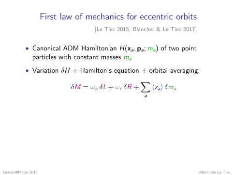
First law of mechanics for eccentric orbits[Le Tiec 2015, Blanchet & Le Tiec 2017]

• Canonical ADM Hamiltonian H(xa,pa;ma) of two pointparticles with constant masses ma

• Variation δH + Hamilton’s equation + orbital averaging:

δM = ωφ δL + ωr δR +∑a

〈za〉 δma

• First integral associated with the variational first law:

M = 2 (ωφL + ωrR) +∑a

〈za〉ma

• These relationships are valid up to at least 4PN order,despite the tail-induced non-local-in-time dynamics


EOB dynamics beyond circular motion

m2

m1+ m

2

EOB

m1

H H (A,D,Q)real eff

• Conservative EOB dynamics determined by “potentials”

A = 1− 2M/r + ν a(r) + · · ·D = 1 + ν d(r) + · · ·Q = ν q(r) p4

r + · · ·

• Functions a(r), d(r) and q(r) controlled by 〈z〉GSF(Ωr ,Ωφ)


EOB dynamics beyond circular motion[Akcay & van de Meent 2016]

Numerical

Δd ISCO(v)

d ISCO(v)

d BDG6.5 pN

(v)

d BDGPade

(v)

0.01 0.05 0.1 0.15 ISCOv

0.6

0.2

0.4

d(v)

0.15 0.16 ISCO0.4

0.5

0.6


EOB dynamics beyond circular motion[Akcay & van de Meent 2016]

Numerical

ΔqISCO(v)

qISCO(v)

qDJS4 pN

(v)

0.01 0.05 0.1 0.15 ISCOv

0.2

0.3

0.1

0.4

q(v)

0.125 0.15 0.16 ISCO

0.3

0.15

0.45


Two-body scattering and EOB mappings[Damour 2016, Vines 2017]

M ↔ m1+m2 µ↔ m1m2

ME ↔ µ+

E 2 −M2

2Ma↔ M

E(a1+a2)

EOB energy map new spin map



M ↔ m1+m2

µ↔ m1m2

ME ↔ µ+

E 2 −M2

2Ma↔ M

E(a1+a2)




M ↔ m1+m2 µ↔ m1m2

M

E ↔ µ+E 2 −M2

2Ma↔ M

E(a1+a2)




M ↔ m1+m2 µ↔ m1m2

ME ↔ µ+

E 2 −M2

2M

a↔ M

E(a1+a2)

EOB energy map

new spin map



M ↔ m1+m2 µ↔ m1m2

ME ↔ µ+

E 2 −M2

2Ma↔ M

E(a1+a2)



Prospects

• Extend the knowledge of the GW phase to the 4.5PN order

• Amplitude corrections, higher order modes, eccentricity andspin effects on the waveform

• PN waveform in well-motivated alternative theories of gravity

• Compare PN predictions to upcoming 2nd order GSF results

• Extend and exploit:

(i) First laws of binary mechanics

(ii) EOB mappings in PM gravity


Further reading

Review articles

• Gravitational radiation from post-Newtonian sources. . .L. Blanchet, Living Rev. Rel. 17, 2 (2014)

• Post-Newtonian methods: Analytic results on the binary problemG. Schafer, in Mass and motion in general relativityEdited by L. Blanchet et al., Springer (2011)

• The post-Newtonian approximation for relativistic compact binariesT. Futamase and Y. Itoh, Living Rev. Rel. 10, 2 (2007)

Topical books

• Gravity: Newtonian, post-Newtonian, relativisticE. Poisson and C. M. Will, Cambridge University Press (2015)

• Gravitational waves: Theory and experimentsM. Maggiore, Oxford University Press (2007)


post-newtonian and post-minkowskian approximations

Documents