preface - british columbia
TRANSCRIPT

Field Manual forDescribing Terrestrial Ecosystems
B.C. Ministry of Environment, Lands, and ParksB.C. Ministry of Forests
Land ManagementHandbook NUMBER
ISSN 0229-1622
1998
25

Field Manual for
Describing Terrestrial Ecosystems
B.C. Ministry of Environment, Lands, and ParksB.C. Ministry of Forests
1998

Canadian Cataloguing in Publication Data
Main entry under title:Field manual for describing terrestrial ecosystems
(Land management handbook, ISSN 0229-1622 ; 25)
Co-published by B.C. Ministry of Forests andB.C. Ministry of Environment, Lands and Parks.ISBN 0-7726-3604-4
1. Ecological surveys - Handbooks, manuals, etc. 2.Ecological surveys - British Columbia - Handbooks,manuals, etc. 3. Forest surveys - British Columbia -Handbooks, manuals, etc. 4. Forest site quality -British Columbia - Handbooks, manuals, etc. I.British Columbia. Ministry of Environment, Lands andParks. II. British Columbia. Ministry of Forests. III.Series.
QH541.15.S95F53 1998 577'.09711 C98-960184-6
1998 Province of British Columbia
Co-Published by theResources Inventory BranchB.C. Ministry of Environment, Lands and ParksandResearch BranchB.C. Ministry of Forests712 Yates StreetVictoria, B.C. V8W 9C2
Copies of this and other MInistry of Foreststitles are available from Crown Publications Inc.,546 Yates Street, Victoria, B.C. V8W 1K8.
Preface
How to use this manualThis manual has been prepared to assist field surveyors in thecompletion of the Ecosystem Field Forms, including site, soil,vegetation, mensuration, wildlife habitat assessment, tree attributesfor wildlife, and coarse woody debris data forms. These are a seriesof forms for the collection of ecological data in British Columbia.
The field manual is organized by section—one for each data form.The forms, as a package, are called Ecosystem Field Forms (FS882)and are numbered as follows:
Site Description FS882(1) ........................................................ SITESoil Description FS882(2) ........................................................ SOILVegetation FS882(3) ................................................................. VEGMensuration FS882(4) .............................................................. MENSWildlife Habitat Assessment FS882(5) ................................. WHATree Attributes for Wildlife FS882(6) .................................... TAWCoarse Woody Debris FS882(7) ............................................. CWDReferences .................................................................................. REFGround Inspection (included as an insert) .......................... GIF
The forms are designed to be used in various inventories, e.g.,ecosystem classification, terrestrial ecosystem mapping, andwildlife habitat assessment. Not all the data fields on all the formswill be completed on every sample plot. Rather, project objectiveswill determine which forms and fields need to be completed.Likewise, project objectives will determine where and how plotsare located.
•iii•

The field manual follows Describing Ecosystems in the Field (Luttmerding etal. 1990), however, it has been updated to accommodate new inventoryrequirements and standards. The forms evolved from the B.C. Ministry ofForests Ecological Classification Reconnaissance Form, the larger moredetailed forms in Luttmerding et al. (1990), and the Vegetation ResourceInventory forms (Resources Inventory Committee 1997).
The size of sample plots has not been identified in this field manual. Inmost cases, a plot size of 400 m2 is considered adequate, however, inspecies-poor ecosystems, the plot size could be smaller (e.g., somewetlands, grasslands, dense forests). Plot shape can be rectangular, square,or circular, but is usually consistent for a project.As this is a field manual, the descriptions have been kept as brief aspossible. Other supporting references, such as Luttmerding et al. (1990),Green et al. (1993), Howes and Kenk (1997), and Agriculture Canada ExpertCommittee on Soil Survey (1998), among others, will be required if theuser is not already familiar with their contents. See references (Section 8)for a complete list of complementary documents.
•iv•
Acknowledgements
This field manual was compiled and edited from material from manysources. As such, there are no easily identifiable authors. Most of thecompilation and editing work was completed by Del Meidinger, RickTrowbridge, Anne Macadam, and Calvin Tolkamp. However, manyothers kindly contributed their time and current information, including:John Parminter, Bob Maxwell, Scott Smith, Charles Tarnocai, and WillMackenzie. Assistance in editing various versions was provided by TedLea, Barb von Sacken, Carmen Cadrin, Larry Lacelle, Tina Lee andArman Mirza. Greg Britton contributed valuable suggestions concerningdata formats and codes.
Contributors to other documents and forms also assisted with this fieldmanual by their work on classifications, procedures, diagrams, figures,tables, or design. All the manuals, reports, and publications used toprepare this field manual are listed in the References section. Theauthors, compilers, and contributors to these primary sources ofinformation are gratefully acknowledged. Their unselfish work has madethis field guide possible.
Many others contributed to the production of the field guide. LouiseGronmyr and Christina Stewart typed the original material fromDescribing Ecosystems in the Field. Anette Thingsted assisted with anearlier draft. Susan Bannerman prepared an extremely useful Englishand format edit. Tetrad Creative Services and Greg Britton prepared thecamera-ready version.
The compilers of this field manual greatly appreciate everyone’scontributions.
Financial assistance for preparing this guide has been provided by theB.C. Ministry of Forests, B.C. Ministry of Environment, Lands, andParks, and particularly, Forest Renewal B.C.
•v•

•vi•

Contents
Site Description Form ............................................................... 3Field Procedure .......................................................................... 4Completing the Form ............................................................... 5
1. Date ................................................................................... 52. Plot Number .................................................................... 53. Project ID ......................................................................... 54. Field Number .................................................................. 55. Surveyor(s) ...................................................................... 66. General Location............................................................. 67. Forest Region .................................................................. 68. Map Sheet ........................................................................ 69. UTM Zone ........................................................................ 6
10. Latitude/Longitude or Northing/Easting .................. 611. Air Photo Number ......................................................... 712. X/Y Co-ordinates ............................................................ 713. Map Unit .......................................................................... 714. Site Diagram .................................................................... 715. Plot Representing ........................................................... 816. Biogeoclimatic Unit ......................................................... 817. Site Series ......................................................................... 818. Transition/Distribution Codes ..................................... 819. Ecosection ........................................................................ 920. Moisture Regime ............................................................ 921. Nutrient Regime ............................................................. 1122. Successional Status .......................................................... 1123. Structural Stage ............................................................... 1624. Realm/Class .................................................................... 1925. Site Disturbance .............................................................. 2226. Photo Roll and Frame Numbers .................................. 2527. Elevation .......................................................................... 2528. Slope ................................................................................. 2529. Aspect ............................................................................... 2530. Mesoslope Position......................................................... 2531. Surface Topography ....................................................... 26
1 SITE DESCRIPTION
Page

•2•
32. Exposure Type ................................................................. 2733. Surface Substrate ............................................................ 2934. Notes ................................................................................ 30
Appendices1.1 Biogeoclimatic Units of British Columbia ................... 311.2 Ecosections of British Columbia ................................... 38
Tables1.1 Soil moisture regime classes ......................................... 101.2 Nutrient regime classes and relationships between
regime and site properties ............................................ 12
Figures1.1 Examples of site diagrams .......................................... 71.2 Stand structure modifiers .............................................. 201.3 Mesoslope position ......................................................... 26
Page
•3•
SIT
E D
IAG
RA
M
FIE
LD N
O.
SU
RV
EY
OR
(S)
SITE DESCRIPTION
SIT
E IN
FO
RM
ATIO
N
NO
TE
S
GE
NE
RA
LLO
CAT
ION
UT
MZ
ON
EM
AP
SH
EE
T
Y C
O-O
RD
.
SU
BS
TR
AT
E (
%)
OR
G. M
ATT
ER
RO
CK
S
DE
C. W
OO
DM
INE
RA
L S
OIL
BE
DR
OC
KW
AT
ER
EX
PO
S.
TY
PE
SIT
ED
IST
UR
B.
AS
PE
CT
PR
OJE
CT
ID.
LA
T./
NO
RT
H.
m.
%o
ME
SO
SLO
PE
PO
S.
SU
RFA
CE
TO
PO
G.
FO
RE
ST
RE
GIO
N
AIR
PH
OT
ON
O.
PLO
TR
EP
RE
SE
NT
ING
BG
CU
NIT
ELE
V.
X C
O-O
RD
.M
AP
UN
IT
LON
G./
EA
ST.
SIT
ES
ER
IES
TR
AN
S./
DIS
TR
IB.
ST
RU
CT.
STA
GE
RE
ALM
/C
LAS
SM
OIS
TU
RE
RE
GIM
E
SLO
PE
PH
OT
OR
OLL
FR
AM
EN
OS
.
EC
OS
YS
TE
M F
IELD
FO
RM
EC
OS
EC
TIO
N
NU
TR
IEN
TR
EG
IME
SU
CC
ES
S.
STA
TU
S
MIN
IST
RY
OF
FO
RE
ST
SB
C E
NV
IRO
NM
EN
T
FS
882
(1)
HR
E 9
8/5
LOC
ATIO
N
PLO
T N
O.
DATE
Y
M
D
54
3
6 20
16
15
11
78
21
17
12
9
22
18
13
10
23
19 24
14
2526
32
33
3130
29
34
2827
12
•4•
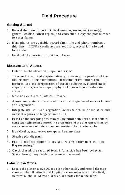
Field Procedure
Getting Started
1 . Record the date, project ID, field number, surveyor(s) name(s),general location, forest region, and ecosection. Copy the plot numberto other forms.
2 . If air photos are available, record flight line and photo numbers atthis time. If GPS co-ordinates are available, record latitude andlongitude.
3 . Establish the location of plot boundaries.
Measure and Assess
1 . Determine the elevation, slope, and aspect.
2 . Traverse the entire plot systematically, observing the position of theplot relative to the surrounding landscape, microtopographicfeatures, and the composition of surface substrates. Record meso-slope position, surface topography and percentage of substrateclasses.
3 . Note any evidence of site disturbance.
4 . Assess successional status and structural stage based on site factorsand vegetation.
5 . Integrate site, soil, and vegetation factors to determine moisture andnutrient regime and biogeoclimatic unit.
6. Based on the foregoing assessments, determine site series. If the site iscomplex, estimate and record the proportion of the plot represented byeach site series and determine the transition/distribution code.
7. If applicable, enter exposure type and realm/class.
8. Sketch a plot diagram.
9 . Enter a brief description of key site features under Item 15, "PlotRepresenting."
10. Check that all the required form information has been collected.Strike through any fields that were not assessed.
Later in the Office
1. Locate the plot on a 1:20 000 map (or other scale), and record the mapsheet number. If latitude and longitude were not entered in the field,determine the UTM zone and co-ordinates from the map.

•5•
2 . Compare elevation recorded in the field with that indicated on atopographic map, and adjust if appropriate.
3 . Locate the plot on an air photo and determine X and Y co-ordinates.
4 . Check again that all the required information has been collected andnoted on the form.
Refer to the following guides for more information:
• Ministry of Forests (MOF) regional field guides to site identification andinterprepation
• Describing Ecosystems in the Field (DEIF) manual (Luttmerding et al. 1990)
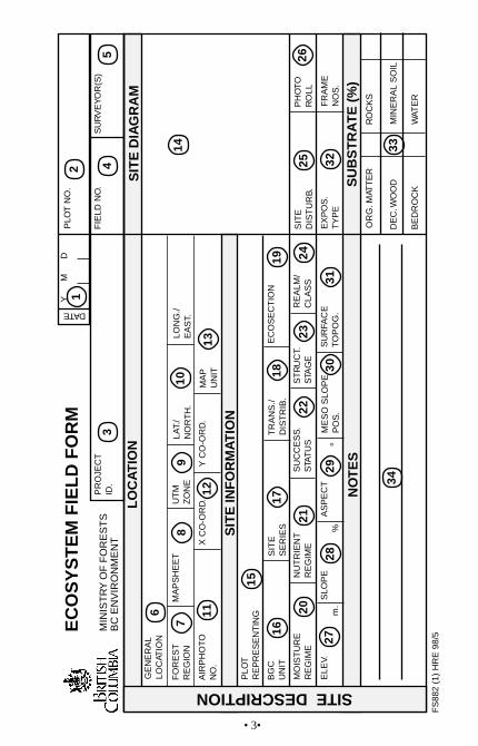
Completing the FormNumbered items below refer to circled numbers on the ecosystem fieldform shown at the beginning of this section. A recommended sequence forcompleting the form is described under "Field Procedure."
1. DateEnter two-digit codes for year, month, and day.
2. Plot NumberThis is the number printed in red in the top right corner of form. Itprovides a unique plot identifier for data management purposes. Recordthis number on all other forms completed for the plot.
3. Project IDEnter a descriptor that connotes the type of project and provides informa-tion about the subject or location of the project. For example:
• ecosystem mapping projects: TEM_BeaverCove
• species inventory: SPP_Woss
• site series classification: BEC_SBSwk1
• wildlife habitat inventory: WHI_grizzly
• site index: SIBEC_Morice
4. Field NumberUse up to eight characters to further identify the plot according to theneeds of the specific project.

•6•
5. Surveyor(s)Record the first initial and last name of each person involved in describ-ing the site.
6. General LocationDescribe the location of the plot relative to natural features such asmountains or bodies of water and permanent structures such askilometre signs on main roads.
• Select points of reference that are unlikely to change and arenamed on maps or are otherwise easily identified.
• Include compass bearings and distances (measured or estimated),where possible.
• More detailed access information may be recorded under Item 34,"Notes."
7. Forest RegionThis information can be useful for sorting plot data. Use the followingcodes:CAR = CaribooKAM = KamloopsNEL = NelsonPG = Prince GeorgePR = Prince RupertVAN = Vancouver
8. Map SheetUse the B.C. Geographic System to identify the map sheet on which theplot is located (e.g., 93H015). The preferred map scale is 1:20,000.
9. UTM ZoneIf using the UTM system to indicate precise plot location, enter the UTMzone number indicated on the map sheet (8–11 within British Columbia).The present standard for UTM data is NAD83. Most new maps follow thisstandard. Older maps, and some new maps use NAD27 which will causesignificant location errors if it is mistaken for NAD83.
10. Latitude/Longitude or Northing/EastingDetermine the precise location of plot using the best available topographicbase map. Latitude and longitude may also be determined using GPS.While either system may be used, the UTM system is recommended if co-ordinates are determined from a map.• For latitude and longitude, note degrees (°), minutes (‘), and
seconds (“).
• For UTM system, record northing and easting (NAD83).
•7•
11. Air Photo NumberRecord the flight line and air photo number.
12. X/Y Co-ordinatesUsing a plastic air photo grid overlay (2M–79), record values of X and Yco-ordinates for the intersecting lines closest to the plot location. Placethe grid over the photograph with photo number viewed upright and theorigin of grid axes aligned with the lower left-hand corner. Be sure toalign centre and feducial points (points at corners or centre of each sideof photograph).
13. Map UnitIf the plot is part of a mapping project, enter coding for the terrestrialecosystem (TEM) or other map unit (eg., soils, terrain, etc.). TEM unitcoding is as follows:
Site series Site modifier Structural stageSS mm #xx
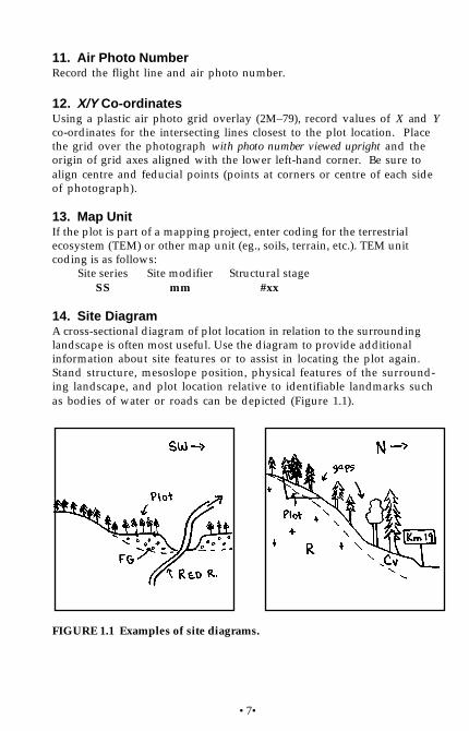
14. Site DiagramA cross-sectional diagram of plot location in relation to the surroundinglandscape is often most useful. Use the diagram to provide additionalinformation about site features or to assist in locating the plot again.Stand structure, mesoslope position, physical features of the surround-ing landscape, and plot location relative to identifiable landmarks suchas bodies of water or roads can be depicted (Figure 1.1).
FIGURE 1.1 Examples of site diagrams.
•8•
15. Plot RepresentingBriefly characterize the site. If the plot was not selected randomly orsystematically, describe the key attributes for which it was chosen.For example:
• Open Pl stand; kinnikinnick, lichens on FG terrace
• Young highly productive Fd stand on zonal site
• Sxw– horsetail–ladyfern, Hydromor, Humic Gleysol, on floodplain
16. Biogeoclimatic UnitEnter a code for the biogeoclimatic zone and subzone. Include variant andphase where applicable. Ministry of Forests maps and regional field guidesto site identification and interpretation are the best sources of information.A current listing of codes is given in Appendix 1.1.
• In areas distinctly transitional between two recognized biogeoclimaticunits, enter the code for the dominant unit here and mark with anasterisk (*). Identify other unit and explain under "Notes" (Item 34).
17. Site SeriesEnter a two-digit site series code and a letter code for site series phases,where recognized, from the appropriate MOF regional field guide to siteidentification and interpretation. Note the following special cases:
• If two or more distinct site series are present, list in order of predomi-nance, followed by the proportion of the plot represented by each inpercent. For example: 01a (70%), 05 (30%).
• Where site characteristics are uniform, but distinctly transitionalbetween two recognized site series, indicate with a dash(e.g., 01a–05).
• If the ecosystem does not resemble a recognized site series, leave thisfield blank, and explain under "Notes".
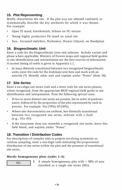
18. Transition / Distribution CodesFor descriptions of complex sites in projects involving systematic orrandom sampling, enter a one-digit code indicating the proportionaldistribution of site series within the plot and the presence of transitionalsite series.
Mostly homogeneous plots (codes 1–3):
1 A simple homogeneous plot with > 98% of areaclassified as a single site series (SS1).
SS1

•9•
2 A homogeneous plot with > 90% of the areaclassified as SS1; however, site characteristics aregrading slightly toward SS2. Less than 10% of thearea is distinctly SS2.
3 A homogeneous plot, but classification isintermediate between SS1 and SS2.
Transitional from one edge of the plot to the other (code 4):
4 Gradual transition from SS1 at one edge of plot toSS2 at other edge, or from SS2 to SS3, with SS1 beingthe modal site series. In the latter case, SS1 usuallyrepresents > 50% of plot.
Two or more distinct site series present (codes 5–8):
5 Two or more distinct site series present, with SS1representing > 70% of plot area.
6 Two or more distinct site series, with SS1representing 40–69% of plot area.
7 Two distinct areas in the plot: SS1 represents > 50%of area, and remainder is intermediate between SS2and SS3.
8 Two distinct areas in the plot: > 50% is intermediatebetween SS1 and SS2, and remainder is SS3.
19. EcosectionEnter a three-letter code for the ecosection. See Appendix 1.2 for a currentlisting of codes.
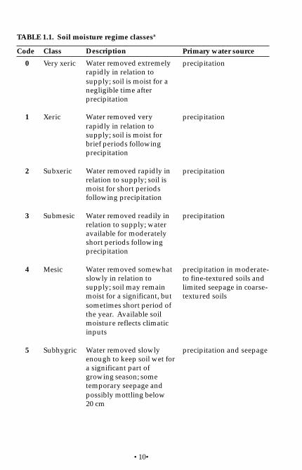
20. Moisture RegimeEnter a code (0–8) for moisture regime. Base the assessment on environ-mental factors, soil properties, and indicator plants relative to other siteswithin same biogeoclimatic unit. Classes are listed with brief descriptionsin Table 1.1. Note the following special cases:
• If two or more areas of the plot have a distinctly different moistureregime, enter codes for the dominant and largest sub-dominant class,with the sub-dominant class in parentheses (e.g., 4 (5)).
• If a wide range of moisture regimes is present, list the dominantand sub-dominant class, followed by the range (e.g. 4 (5), 4–6).
• Where moisture regime is distinctly transitional between two classes,indicate with “+” or “-” (e.g., 4+).
SS1(SS2)
SS1–SS2
SS1 SS2
SS1 SS2
SS3SS2SS1
SS2–SS3SS1
SS3SS1–SS2
•10•
TABLE 1.1. Soil moisture regime classesa
Description
Water removed extremelyrapidly in relation tosupply; soil is moist for anegligible time afterprecipitation
Water removed veryrapidly in relation tosupply; soil is moist forbrief periods followingprecipitation
Water removed rapidly inrelation to supply; soil ismoist for short periodsfollowing precipitation
Water removed readily inrelation to supply; wateravailable for moderatelyshort periods followingprecipitation
Water removed somewhatslowly in relation tosupply; soil may remainmoist for a significant, butsometimes short period ofthe year. Available soilmoisture reflects climaticinputs
Water removed slowlyenough to keep soil wet fora significant part ofgrowing season; sometemporary seepage andpossibly mottling below20 cm
Code Class
0 Very xeric
1 Xeric
2 Subxeric
3 Submesic
4 Mesic
5 Subhygric
Primary water source
precipitation
precipitation
precipitation
precipitation
precipitation in moderate-to fine-textured soils andlimited seepage in coarse-textured soils
precipitation and seepage
•11•
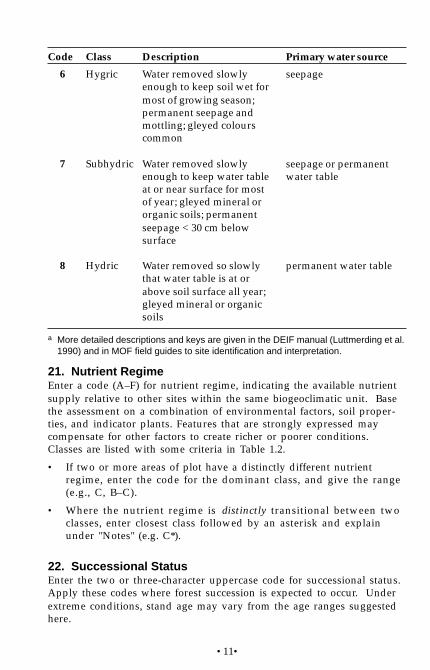
a More detailed descriptions and keys are given in the DEIF manual (Luttmerding et al.1990) and in MOF field guides to site identification and interpretation.
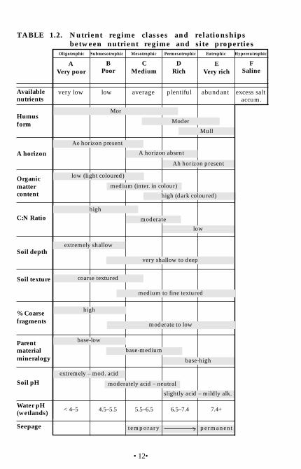
21. Nutrient RegimeEnter a code (A–F) for nutrient regime, indicating the available nutrientsupply relative to other sites within the same biogeoclimatic unit. Basethe assessment on a combination of environmental factors, soil proper-ties, and indicator plants. Features that are strongly expressed maycompensate for other factors to create richer or poorer conditions.Classes are listed with some criteria in Table 1.2.
• If two or more areas of plot have a distinctly different nutrientregime, enter the code for the dominant class, and give the range(e.g., C, B–C).
• Where the nutrient regime is distinctly transitional between twoclasses, enter closest class followed by an asterisk and explainunder "Notes" (e.g. C*).
22. Successional StatusEnter the two or three-character uppercase code for successional status.Apply these codes where forest succession is expected to occur. Underextreme conditions, stand age may vary from the age ranges suggestedhere.
Code Class
6 Hygric
7 Subhydric
8 Hydric
Description
Water removed slowlyenough to keep soil wet formost of growing season;permanent seepage andmottling; gleyed colourscommon
Water removed slowlyenough to keep water tableat or near surface for mostof year; gleyed mineral ororganic soils; permanentseepage < 30 cm belowsurface
Water removed so slowlythat water table is at orabove soil surface all year;gleyed mineral or organicsoils
Primary water source
seepage
seepage or permanentwater table
permanent water table
•12•
AVery poor
BPoor
CMedium
DRich
EVery rich
FSaline
Oligotrophic
very low low average plentiful abundant excess saltaccum.
Submesotrophic Mesotrophic Permesotrophic Eutrophic Hypereutrophic
% Coarsefragments
Soil depth
A horizon
Humusform
Availablenutrients
Mor
Ae horizon present
Moder
Mull
A horizon absent
Ah horizon present
low (light coloured)
medium (inter. in colour)
high (dark coloured)
high
moderate
low
extremely shallow
very shallow to deep
coarse textured
medium to fine textured
high
moderate to low
base-low
base-medium
base-high
extremely – mod. acid
moderately acid – neutral
slightly acid – mildly alk.
< 4–5 4.5–5.5 5.5–6.5 6.5–7.4 7.4+
temporary permanent
Organicmattercontent
C:N Ratio
Soil texture
Parentmaterialmineralogy
Soil pH
Water pH(wetlands)
Seepage
TABLE 1.2. Nutrient regime classes and relationshipsbetween nutrient regime and site properties
•13•
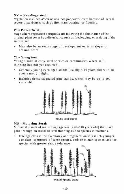
Maturing seral stand
Young seral stand
NV = Non-Vegetated:Vegetation is either absent or less than five percent cover because of recentsevere disturbances such as fire, mass-wasting, or flooding.
PS = Pioneer Seral:Stage where vegetation occupies a site following the elimination of theoriginal plant cover by a disturbance such as fire, logging, or scalping of thesoil surface.
• May also be an early stage of development on talus slopes orerosion scars.
YS = Young Seral:Young stands of early seral species or communities where self-thinning has not yet occurred.
• Generally young even-aged stands (usually < 60 years old) with aneven canopy height.
• Includes dense stagnated pine stands, which may be up to 100years old.
MS = Maturing Seral:Mid-seral stands of mature age (generally 60–140 years old) that havegone through an initial natural thinning due to species interactions.
• One age class in the overstorey and regeneration in a much youngerage class, composed of same species, and/or climax species, and/orspecies with greater shade tolerance.
•14•
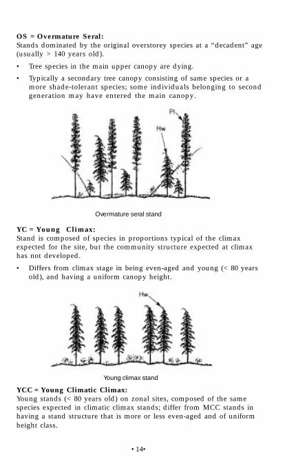
OS = Overmature Seral:Stands dominated by the original overstorey species at a “decadent” age(usually > 140 years old).
• Tree species in the main upper canopy are dying.
• Typically a secondary tree canopy consisting of same species or amore shade-tolerant species; some individuals belonging to secondgeneration may have entered the main canopy.
Young climax stand
Overmature seral stand
YCC = Young Climatic Climax:Young stands (< 80 years old) on zonal sites, composed of the samespecies expected in climatic climax stands; differ from MCC stands inhaving a stand structure that is more or less even-aged and of uniformheight class.
YC = Young Climax:Stand is composed of species in proportions typical of the climaxexpected for the site, but the community structure expected at climaxhas not developed.
• Differs from climax stage in being even-aged and young (< 80 yearsold), and having a uniform canopy height.

•15•
YEC = Young Edaphic Climax:Young stands (usually < 80 years old) composed of the same speciesexpected at climax on a site edaphically different from a “zonal” site.
• Differs in stand structure from the MEC in being more or less even-agedand of uniform height class.
• Examples include a young spruce stand on a wet site, or a youngDouglas-fir stand on a dry, south-facing slope.
MC = Maturing Climax:Stands composed of species expected to be present in the climax stand; standhas undergone natural thinning, gaps have been created, and a structuresimilar to that expected at climax has developed.
• Differs from the YC in having a better-developed understorey and amore or less continuous age and height class distribution, al-though a gap may exist between the older or upper class and thenext class.
• Some remnants of the earlier stand may remain, but they should nothave any effect on the density or structure of the stand. Removal ofa tree would not cause a significant response in the growth orestablishment of the climax trees.
Maturing climax stand
MCC = Maturing Climatic Climax:Stands on zonal sites composed of the species representative of theclimatic climax, and approaching a continuous age and height classdistribution.
• There may be a gap between the main canopy and the continuousage and height class distribution of the regeneration.
• Stands are at least 80–120 years old, but usually much older.
•16•
MEC = Maturing Edaphic Climax:Differs from MCC stands in species composition and site conditions(occurs on azonal sites); soil properties differ primarily in terms of soilmoisture and nutrient regime.
• Species differences may be in stand or understorey.
• Examples include grassland communities on coarse-textured or shallowsoils; spruce–horsetail communities on floodplains; bogs and fens inlarge depressional areas; cedar–devil’s club communities on moist, richsites in a BGC unit where cedar–hemlock–oakfern communities occuron zonal sites.
DC = Disclimax:A self-perpetuating community that strongly differs in species compositionfrom the edaphic or climatic climax expected for the site; normal successionhas been arrested by an external physical or anthropogenic factor.
• Results from changes to the physical characteristics of the site, associatedwith disturbances such as fire, intensive grazing, or avalanche.
NOTE: The codes EC or CC, for Edaphic Climax or Climatic Climax, maybe used where it is difficult to determine whether the successional status is“young” or “maturing.”
23. Structural Stage 1
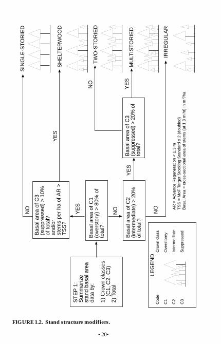
In the assessment of structural stage, structural features and age criteriashould be considered. Use numeric and lowercase alphabetic codes unlessotherwise directed. Modifiers for structural stage (Figure 1.2) and standcomposition are optional. Separate modifier codes from the structural stagecode with a slash (e.g., 7/mC; 3b/D). Uppercase codes in parentheses areused in Vegetation Resources Inventory (Resource Inventory Committee,1997).
Post-disturbance stages, or environmentally limited structuraldevelopment:
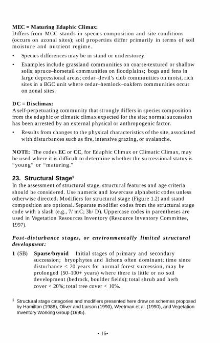
1 (SB) Sparse/bryoid Initial stages of primary and secondarysuccession; bryophytes and lichens often dominant; time sincedisturbance < 20 years for normal forest succession, may beprolonged (50–100+ years) where there is little or no soildevelopment (bedrock, boulder fields); total shrub and herbcover < 20%; total tree cover < 10%.
1 Structural stage categories and modifiers presented here draw on schemes proposedby Hamilton (1988), Oliver and Larson (1990), Weetman et al. (1990), and VegetationInventory Working Group (1995).

•17•
1a (SP) Sparse – less than 10% vegetation cover; or
1b (BR) Bryoid – bryophyte and lichen-dominated communi-ties (> 50% of total vegetation cover).
Stand initiation stages or environmentally induced structural development:
2 (H) Herb Early successional stage or herb communities maintainedby environmental conditions or disturbance (e.g., snow fields,avalanche tracks, wetlands, flooding, grasslands, intensivegrazing, intense fire damage); dominated by herbs (forbs,graminoids, ferns); some invading or residual shrubs and treesmay be present; tree cover < 10%, shrubs < 20% or < 33% of totalcover, herb-layer cover > 20%, or > 33% of total cover; time sincedisturbance < 20 years for normal forest succession; many non-forested communities are perpetually maintained in this stage.
2a (FO) Forb-dominated – includes non-graminoid herbs andferns;
2b (GR) Graminoid-dominated – includes grasses, sedges,reeds, and rushes;
2c (AQ) Aquatic – floating or submerged; does not includesedges growing in marshes with standing water(classed as 2b); or
2d (DS) Dwarf shrub-dominated – dominated by dwarfwoody species such as Arctostaphylos alpina, Salixreticulata, Rhododendron lapponicum, Cassiope tetragona(see Table 3.1 in Vegetation section).
3 (SH) Shrub/Herb Early successional stage or shrub communitiesmaintained by environmental conditions or disturbance;dominated by shrubby vegetation; seedlings and advanceregeneration may be abundant; tree cover < 10%, shrub cover >20% or > 33% of total cover.
3a (LS) Low shrub – dominated by shrubby vegetation < 2 mtall; seedlings and advance regeneration may beabundant; time since disturbance < 20 years for normalforest succession; may be perpetuated indefinitely byenvironmental conditions or disturbance; or
3b (TS) Tall shrub – dominated by shrubby vegetation thatis 2–10 m tall; seedlings and advance regenerationmay be abundant; time since disturbance < 40 years fornormal forest succession; may be perpetuatedindefinitely.
•18•
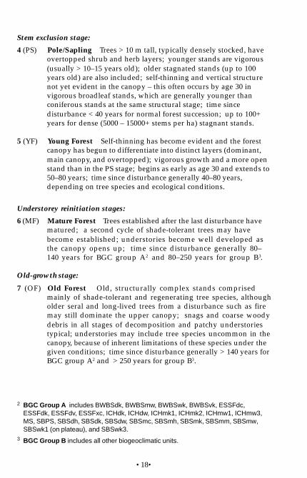
Stem exclusion stage:
4 (PS) Pole/Sapling Trees > 10 m tall, typically densely stocked, haveovertopped shrub and herb layers; younger stands are vigorous(usually > 10–15 years old); older stagnated stands (up to 100years old) are also included; self-thinning and vertical structurenot yet evident in the canopy – this often occurs by age 30 invigorous broadleaf stands, which are generally younger thanconiferous stands at the same structural stage; time sincedisturbance < 40 years for normal forest succession; up to 100+years for dense (5000 – 15000+ stems per ha) stagnant stands.
5 (YF) Young Forest Self-thinning has become evident and the forestcanopy has begun to differentiate into distinct layers (dominant,main canopy, and overtopped); vigorous growth and a more openstand than in the PS stage; begins as early as age 30 and extends to50–80 years; time since disturbance generally 40–80 years,depending on tree species and ecological conditions.
Understorey reinitiation stages:
6 (MF) Mature Forest Trees established after the last disturbance havematured; a second cycle of shade-tolerant trees may havebecome established; understories become well developed asthe canopy opens up; time since disturbance generally 80–140 years for BGC group A2 and 80–250 years for group B3.
Old-growth stage:
7 (OF) Old Forest Old, structurally complex stands comprisedmainly of shade-tolerant and regenerating tree species, althougholder seral and long-lived trees from a disturbance such as firemay still dominate the upper canopy; snags and coarse woodydebris in all stages of decomposition and patchy understoriestypical; understories may include tree species uncommon in thecanopy, because of inherent limitations of these species under thegiven conditions; time since disturbance generally > 140 years forBGC group A2 and > 250 years for group B3.
2 BGC Group A includes BWBSdk, BWBSmw, BWBSwk, BWBSvk, ESSFdc,ESSFdk, ESSFdv, ESSFxc, ICHdk, ICHdw, ICHmk1, ICHmk2, ICHmw1, ICHmw3,MS, SBPS, SBSdh, SBSdk, SBSdw, SBSmc, SBSmh, SBSmk, SBSmm, SBSmw,SBSwk1 (on plateau), and SBSwk3.
3 BGC Group B includes all other biogeoclimatic units.
•19•
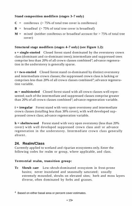
Stand composition modifiers (stages 3–7 only)
C = coniferous (> 75% of total tree cover is coniferous)
B = broadleaf (> 75% of total tree cover is broadleaf)
M = mixed (neither coniferous or broadleaf account for > 75% of total treecover)
Structural stage modifiers (stages 4–7 only) (see Figure 1.2):
s = single-storied Closed forest stand dominated by the overstorey crownclass (dominant and co-dominant trees); intermediate and suppressed treescomprise less than 20% of all crown classes combined4; advance regenera-tion in the understorey is generally sparse.
t = two-storied Closed forest stand co-dominated by distinct overstoreyand intermediate crown classes; the suppressed crown class is lacking orcomprises less than 20% of all crown classes combined4; advance regenera-tion variable.
m = multistoried Closed forest stand with all crown classes well repre-sented; each of the intermediate and suppressed classes comprise greaterthan 20% of all crown classes combined4; advance regeneration variable.
i = irregular Forest stand with very open overstorey and intermediatecrown classes (totalling less than 30% cover), with well developed sup-pressed crown class; advance regeneration variable.
h = shelterwood Forest stand with very open overstorey (less than 20%cover) with well developed suppressed crown class and/or advanceregeneration in the understorey. Intermediate crown class generallyabsent.
24. Realm/ClassCurrently applied to wetland and riparian ecosystems only. Enter thefollowing codes for realm or group, where applicable, and class.
Terrestrial realm, transition group:
Tc Shrub carr Low-shrub-dominated ecosystem in frost-pronebasins; never inundated and seasonally saturated; usuallyextremely mounded, shrubs on elevated sites; herb and moss layersdiverse, often dominated by forbs and grasses.
4 Based on either basal area or percent cover estimates.
•20•
FIGURE 1.2. Stand structure modifiers.
ST
EP
1:
Sum
mar
ize
stan
d ba
sal a
rea
data
by:
1) C
row
n cl
asse
s
(C
1, C
2, C
3)2)
Tot
al
Bas
al a
rea
of C
3(s
uppr
esse
d) >
10%
of to
tal?
and/
orst
ems
per
ha o
f AR
>T
SS
?
Bas
al a
rea
of C
2(in
term
edia
te)
> 2
0%of
tota
l?
Bas
al a
rea
of C
1(o
vers
tory
) >
80%
of
tota
l?
Bas
al a
rea
of C
3(s
uppr
esse
d) >
20%
of
tota
l?
SIN
GLE
-STO
RIE
D
SH
ELT
ER
WO
OD
TW
O-S
TOR
IED
MU
LTIS
TOR
IED
IRR
EG
ULA
R
YE
S
NO NO
YE
S
NO
YE
S
YE
S
NO
Cod
e
C1
C2
C3
Cro
wn
clas
s
Ove
rsto
rey
Inte
rmed
iate
Sup
pres
sed
LEG
EN
D
AR
= A
dvan
ce R
egen
erat
ion
< 1
.3 m
TS
S =
MoF
Tar
get S
tock
ing
Sta
ndar
d x
2 (d
oubl
ed)
Bas
al A
rea
= c
ross
-sec
tiona
l are
a of
ste
ms
(at 1
.3 m
ht)
in m
/ha
2

•21•
Th High meadow Mainly in subalpine and alpine regions; lush forb-richflora; persistent snowpack and prolonged growing season seepage.
Tm Wet meadow Develop on mineral materials; periodically saturated,seldom inundated; diverse community of grasses, low sedges, rushes(Juncus spp.), and forbs.
Ts Saline meadow Occur in dry interior areas of province around salinelakes and in shallow depressions that dry out early in the growingseason; high soil salinities; water table often remains high; salt-tolerantplants.
Terrestrial realm, flood group:
Fl Low bench Flooded at least every other year for moderate periods ofgrowing season; plant species adapted to extended flooding andabrasion; low or tall shrub physiognomy most common.
Fm Middle bench Flooded every 1–6 years for short periods (10–25days); deciduous or mixed forest dominated by species tolerant offlooding and periodic sedimentation; trees occur on elevatedmicrosites.
Fh High bench Only periodically and briefly inundated by high waters,but lengthy subsurface flow in the rooting zone; typically conifer-dominated floodplains of larger coastal rivers.
Ff Fringe Narrow linear communities along open water bodies wherethere is no floodplain; irregular flooding at depth, moderatedmicroclimate, improved light regime (in forested areas), and/ormechanical disturbance by ice.
Wetland realm:
Wb Bog Nutrient-poor peatlands (pH < 4.5) characterized by plantcommunities with a large component of ericaceous shrubs andSphagnum mosses.
Wf Fen Nutrient-medium peatlands fed by ground or surface watersources; dominated by sedges, grasses, reeds, and brown mosses;non-ericaceous shrubs common.
Wm Marsh Mineral wetland that retains shallow surface water formuch of growing season; dominated by emergent sedges,grasses, rushes, or reeds.
Ws Swamp Treed or shrubby mineral wetland; water table at or nearsurface for most of year; if peat present, mainly dark and welldecomposed; high cover of broadleaf or coniferous trees or tall shrubs,forbs and leafy mosses.

•22•
Ww Shallow water Distinct wetlands transitional between wetlands andaquatic ecosystems; characterized by rooted aquatics and standingwater < 2 m deep in mid-summer.
Estuarine Realm:
Em Salt marsh Tidally influenced wetland dominated by graminoidemergents; alternately flooded and exposed with daily tides; bothmarine and fresh water sources.
Ed Salt meadow Tidally influenced herbaceous wetlands in upperintertidal and supratidal zones of estuaries; tidal flooding less frequentthan daily.
Es Salt swamp Treed or shrubby mineral wetlands in brackishlagoons; occasional tidal flooding and subsequent evaporation;waterlogged, highly saline soil.
25. Site DisturbanceNote any events that have caused vegetation and soil characteristics todiffer from those expected at climax for the site. Be as specific as possible,including codes for the category and specific types of disturbance separatedby periods. Record up to three different types of disturbance, separated byslashes. For example, enter L.c./F.l.bb for a clearcut that has been broadcastburned. If existing codes are inadequate, enter an “X” here and explainunder "Notes".
A. Atmosphere-related effects
Use these codes if causative factors are no longer in effect or are isolatedincidents. If effects are ongoing, code as an "Exposure Type" (Item32).e. climatic extremes
co extreme coldht extreme heatgl glaze iceh a severe hailsn heavy snow
p. atmospheric pollutionac acid rainto toxic gases
w. windthrow
B. Biotic effectsb. beaver tree cuttingd. domestic grazing/browsingw. wildlife grazing/browsing (5.1)5
e. excrement accumulation (other than that normally associated withgrazing/browsing) (5.1)5

•23•
i. insects (4.2)5
ki insect killin infestation
p. disease (4.2)5
v. aggressive vegetation
D. Disposalsc. chemical spill or disposale. effluent disposalg. domestic garbage disposalo. oil spill or disposalr. radioactive waste disposal or exposure
F. Firesc. overstorey crown fireg. light surface (ground) firer. repeated light surface firess. severe surface firei. repeated severe surface firesl. burning of logging slash
bb broadcast burnpb piled and burnedwb burned windrows
L. Forest harvestingl. land clearing (includes abandoned agriculture)a. patch cut system
wr with reservesc. clearcut system (if slashburned, see also "Fires")
wr with reserves (patch retention)d. seed tree system
un uniformgr grouped
e . selection systemgr group selectionsi single treest strip
s . shelterwood systemun uniformgr groupst stripi r irregularna naturalnu nurse tree
o. coppice
5 Record type or species under "Notes" using codes given in Appendix 4.2 of theMensuration section or Appendix 5.1 of the Wildlife Habitat Assessment section ofthis manual.
•24•
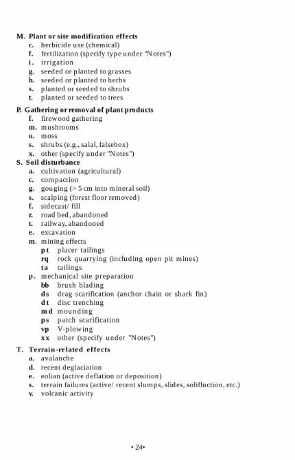
M. Plant or site modification effectsc. herbicide use (chemical)f. fertilization (specify type under "Notes")i . irrigationg. seeded or planted to grassesh. seeded or planted to herbss. planted or seeded to shrubst. planted or seeded to trees
P. Gathering or removal of plant productsf. firewood gatheringm. mushroomso. mosss. shrubs (e.g., salal, falsebox)x. other (specify under "Notes")
S. Soil disturbancea. cultivation (agricultural)c. compactiong. gouging (> 5 cm into mineral soil)s. scalping (forest floor removed)f. sidecast/fillr. road bed, abandonedt. railway, abandonede. excavationm. mining effects
pt placer tailingsrq rock quarrying (including open pit mines)ta tailings
p. mechanical site preparationbb brush bladingds drag scarification (anchor chain or shark fin)dt disc trenchingmd moundingps patch scarificationvp V-plowingxx other (specify under "Notes")
T. Terrain-related effectsa. avalanched. recent deglaciatione. eolian (active deflation or deposition)s. terrain failures (active/recent slumps, slides, solifluction, etc.)v. volcanic activity

•25•
W. Water-related effectsi. inundation (including temporary inundation resulting from beaver
activity)s. temporary seepage (usually artificially induced; excludes
intermittent seepage resulting from climatic conditions)d. water table control (diking, damming)e. water table depression (associated with extensive water extraction
fromwells)
X. Miscellaneous(For other disturbance types, enter “X” and describe under "Notes")
26. Photo Roll and Frame NumbersIf photographs are taken, note the roll and frame numbers.
27. ElevationDetermine in the field using an altimeter. Accuracy of the measurementcan be confirmed by consulting a topographic map. Record in metres withan estimate of accuracy.
28. SlopeRecord percent slope gradient, measured with a clinometer or similarinstrument.
29. AspectRecord the orientation of the slope, measured by compass, in degrees.
• Enter due north as 0°.
• For level ground, enter “999."
30. Mesoslope PositionIndicate the position of plot relative to the localized catchment area(see Figure 1.3).
CR Crest The generally convex uppermost portion of a hill; usuallyconvex in all directions with no distinct aspect.
UP Upper Slope The generally convex upper portion of the slopeimmediately below the crest of a hill; has a specific aspect.
MD Middle Slope Area between the upper and lower slope; thesurface profile is generally neither distinctly concave nor convex;has a straight or somewhat sigmoid surface profile with a specificaspect.
LW Lower Slope The area toward the base of a slope; generally has aconcave surface profile with a specific aspect.

•26•
TO Toe The area demarcated from the lower slope by an abrupt decreasein slope gradient; seepage is typically present.
DP Depression Any area concave in all directions; may be at the base ofa meso-scale slope or in a generally level area.
LV Level Any level meso-scale area not immediately adjacent to a meso-scale slope; the surface profile is generally horizontal and straight withno significant aspect.
31. Surface TopographyNote the general surface shape and the size, frequency, and type ofmicrotopographic features. Describe to the level that best represents whatyou see, separating coding with periods (e.g., code a generally straightsurface that is slightly mounded as ST.sl.mnd and a generallyconcave surface that is relatively flat as CC.smo).
General surface shape:
CC. Concave – surface profile is mainly “hollow” in one or severaldirections
CV. Convex – surface profile is mainly “rounded” like the exterior of asphere
ST. Straight – surface profile is linear, either flat or sloping in onedirection
Size and frequency of microtopographic features:
mc. micro – low relief features (< 0.3 m high) with minimal effect on
Cre
st
Upp
er
Mid
dle
Low
er
Toe
Dep
ress
ion
Leve
l
FIGURE 1.3. Mesoslope position.
•27•
vegetationsl. slightly – prominent features (0.3–1m high) spaced > 7 m apartmd. moderately – prominent features (0.3–1m high) spaced 3–7 m apartst. strongly – prominent features (0.3–1m high) spaced 1–3 m apartsv. severely – prominent features (0.3–1m high) spaced < 1 m apartex. extremely – very prominent features (> 1 m high) spaced > 3 m apartul. ultra – very prominent features (> 1 m high) spaced < 3 m apart
Types of microtopographic features:
cha channelled – incised water tracks or channelsdom domed – raised bogsgul gullied – geomorphic ridge and ravine patternshmk hummocked – mounds composed of organic materialslob lobed – solifluction lobesmnd mounded – mounds composed of mineral materialsnet netted – net vegetation patterns from freeze-thaw action in alpine or
subarctic terrainpol polygonal – polygonal patterns associated with permafrostrib ribbed – wetland pattern with raised ridges perpendicular to
direction of water flowsmo smooth – surface relatively flattus tussocked – associated with tussock-forming graminoids
32. Exposure TypeNote significant localized atmospheric and climate-related factors reflectedin atypical soil and/or vegetation features. If existing codes are inad-equate, enter an “X” and explain under "Notes". If there is no evidence ofexposure to anomalous conditions, enter "NA."
AT Atmospheric toxicity For example, where highly acid or alkalineprecipitation, or chemically toxic fumes from industrial plantsaffect soil chemistry and morphology, and the type and growthform of vegetation.
• Soil indicators – unusually high or low pH values;accumulations of chemicals normally either absent or presentin small quantities.
• Vegetation indicators – defoliated areas; diseased or deadstanding species; presence of several species tolerant toabnormal chemical accumulations.
CA Cold air drainage Downslope areas through which cold airpasses; often grade into frost pockets, but differ in that cold air does
•28•
not accumulate in them. Soil and vegetation indicators are similar tothose for “FR," but the influence of cold temperatures is usually not aspronounced.
FR Frost Cold air accumulation in depressions and valley bottomsassociated with high night-time surface cooling and/or cold airdrainage. Frost pockets are often surrounded by slopes leading to thehigher elevations from which the cold air originates.
• Soil indicators – wet conditions and/or deep organicaccumulations.
• Vegetation indicators – species normally found in colderconditions than those of the general area, such as Abieslasiocarpa in the IDF zone; the presence of frost-hardy shrubsand herbs, such as scrub birch, marsh cinquefoil, and/orshrubby cinquefoil; abundant frost cracks on the trunks oftrees.
IN Insolation Sites subjected to radiant solar heating to a significantlygreater degree than on associated flat or gently sloping ground.Generally on SE, S, and SW aspects with slopes > 20–50%, dependingon climate.
• Soil indicators – weaker than average soil profile development,reflecting a drier environment, or occasionally soil profileswith darker-coloured surface horizons.
• Vegetation indicators – heat-tolerant species; reduced treegrowth; slow or sparse tree regeneration; open crown cover,and tree regeneration in distinct age groups, reflecting ahistory of wetter and drier years.
RN Localized rainshadow Valleys that are protected from theprevailing winds so that they are significantly drier thansurrounding areas.
• Soil indicators – weaker soil development resulting from lessprecipitation, or different soil development because ofsignificantly different vegetation.
• Vegetation indicators – plant communities or speciesindicative of a drier local climate.
SA Saltspray Areas that receive saltspray from a marine environment,affecting the type and growth form of the vegetation, and thechemical and morphological characteristics of the soil.
• Soil indicators – high pH and conductivity, presence of whitesalt accumulations as distinct crystals, and weak profiledevelopment.
• Vegetation indicators – an abundance of salt-tolerantspecies, and slow growth of many species.
SF Fresh water spray Areas adjacent to waterfalls and large rapids that

•29•
receive spray from the rushing water; the resulting vegetation isnoticably different from other areas adjacent to the river or stream.
• Soil indicators – moister soils.• Vegetation indicators – species characteristic of moister sites
are present or more abundant.
SN Snow accumulation Areas that receive significantly more snow thansurrounding areas, which results in different vegetation.
• Soil indicators – poorer soil development resulting from theshorter snow-free period, or moister soils because of the longersnow melt period.
• Vegetation indicators – species adapted to greater snowaccumulations (i.e., resistant to breakage), or a shorter growingseason; or vegetation displaying the effects of a shortergrowing season more than in adjacent areas; or species orcommunities indicative of moister conditions because ofgreater snow melt.
WI Wind Site is directly influenced by strong winds; for example, onexposed mountain tops, along seashores or large lakes, or where “windfunnelling” occurs because of the convergence of valleys in thedirection of wind flow.
• Soil indicators – weak soil development because of scalped(eroded) profiles; evidence of soil erosion on windward sideand deposition on leeside; duning.
• Vegetation indicators – strongly reduced height growth andgnarled growth form with tree tops and branches orienteddownwind; wind-shorn thickets of trees or shrubs (wind-shornsurface of vegetation follows the outline of any objectproviding wind protection).
X Miscellaneous – Describe under "Notes".
33. Surface SubstrateEnter the proportion of the ground surface covered by each class ofsubstrate. The total for all six classes should sum to 100%. Enter “0” if asubstrate class is not present. Classes are defined as follows:
Organic matter Surficial accumulations of organic materials,including the following:
• organic layers > 1 cm thick overlying mineral soil, cobbles,stones, or bedrock;
• layers of decaying wood < 10 cm thick;
• large animal droppings; and
• areas covered by mats of bunchgrasses (mats include L horizons).• Areas of living grass or forb cover where mineral soil is visible

•30•
between stems are classed as mineral soil, as are exposed Ah orAp horizons.
Decaying wood Fallen trees, large branches on the ground surface, andpartially buried stumps with an exposed edge.
• Does not include freshly fallen material that has not yet begun todecompose.
• May be covered with mosses, lichens, liverworts, or other plants.
• If an organic layer has developed over the wood, decaying wood mustbe > 10 cm thick, otherwise it is classed as “organic matter.”
Bedrock Exposed consolidated mineral material.
• May have a partial covering of mosses, lichens, liverworts, orother epilithic plants.
• Does not qualify as bedrock if covered by unconsolidated mineralor organic material > 1 cm in thickness.
Rock (cobbles and stones) Exposed unconsolidated rock fragments> 7.5 cm in diameter.
• May be covered by mosses, lichens, liverworts; or an organic layer < 1 cm in thickness.
• Does not include gravels < 7.5 cm in diameter.
Mineral Soil Unconsolidated mineral material of variable texturenot covered by organic materials.
• May have a partial cover of mosses, lichens, and liverworts.
• Often associated with cultivation, tree tip-ups, active erosion ordeposition, severe fires, trails, or late snow retention areas.
• Includes small cobbles and gravel < 7.5 cm in diameter.
Water Streams, puddles, or areas of open water in bogs or fens.
34. NotesRecord additional information that:
• further characterizes the site;
• assists in finding the plot again;
• explains unusual entries elsewhere on the form; or
• relates to a particular project which is not accommodated elsewhereon the forms.
•31•
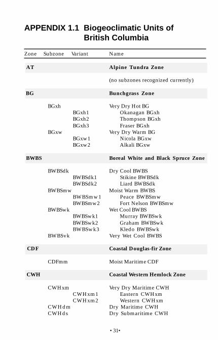
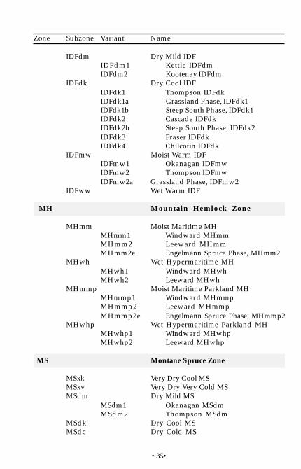
APPENDIX 1.1 Biogeoclimatic Units of British Columbia
Zone Subzone Variant Name
AT Alpine Tundra Zone
(no subzones recognized currently)
BG Bunchgrass Zone
BGxh Very Dry Hot BGBGxh1 Okanagan BGxhBGxh2 Thompson BGxhBGxh3 Fraser BGxh
BGxw Very Dry Warm BGBGxw1 Nicola BGxwBGxw2 Alkali BGxw
BWBS Boreal White and Black Spruce Zone
BWBSdk Dry Cool BWBSBWBSdk1 Stikine BWBSdkBWBSdk2 Liard BWBSdk
BWBSmw Moist Warm BWBSBWBSmw1 Peace BWBSmwBWBSmw2 Fort Nelson BWBSmw
BWBSwk Wet Cool BWBSBWBSwk1 Murray BWBSwkBWBSwk2 Graham BWBSwkBWBSwk3 Kledo BWBSwk
BWBSvk Very Wet Cool BWBS
CDF Coastal Douglas-fir Zone
CDFmm Moist Maritime CDF
CWH Coastal Western Hemlock Zone
CWHxm Very Dry Maritime CWHCWHxm1 Eastern CWHxmCWHxm2 Western CWHxm
CWHdm Dry Maritime CWHCWHds Dry Submaritime CWH

•32•
CWHds1 Southern CWHdsCWHds2 Central CWHds
CWHmm Moist Maritime CWHCWHmm1 Submontane CWHmmCWHmm2 Montane CWHmm
CWHms Moist Submaritime CWHCWHms1 Southern CWHmsCWHms2 Central CWHms
CWHwh Wet Hypermaritime CWHCWHwh1 Submontane CWHwhCWHwh2 Montane CWHwh
CWHwm Wet Maritime CWHCWHws Wet Submaritime CWH
CWHws1 Submontane CWHwsCWHws2 Montane CWHws
CWHvh Very Wet Hypermaritime CWHCWHvh1 Southern CWHvhCWHvh2 Central CWHvh
CWHvm Very Wet Maritime CWHCWHvm1 Submontane CWHvmCWHvm2 Montane CWHvmCWHvm3 Central CWHvm
ESSF Engelmann Spruce – Subalpine Fir Zone
ESSFxc Very Dry Cold ESSFESSFxv Very Dry Very Cold ESSF
ESSFxv1 West Chilcotin ESSFxvESSFxv2 Big Creek ESSFxv
ESSFdk Dry Cool ESSFESSFdku Upper Dry Cool ESSFESSFdc Dry Cold ESSF
ESSFdc1 Okanagan ESSFdcESSFdc2 Thompson ESSFdc
ESSFdv Dry Very Cold ESSFESSFmw Moist Warm ESSF
ESSF mwh Hemlock Phase, ESSFmwESSFmm Moist Mild ESSF
ESSFmm1 Raush ESSFmmESSFmm2 Robson ESSFmm
ESSFmk Moist Cool ESSFESSFmc Moist Cold ESSFESSFmv Moist Very Cold ESSF
ESSFmv1 Nechako ESSFmv
Zone Subzone Variant Name

•33•
ESSFmv2 Bullmoose ESSFmvESSFmv3 Omineca ESSFmvESSFmv4 Graham ESSFmv
ESSFwm Wet Mild ESSFESSFwk Wet Cool ESSF
ESSFwk1 Cariboo ESSFwkESSFwk2 Misinchinka ESSFwk
ESSFwc Wet Cold ESSFESSFwc1 Columbia ESSFwcESSFwc2 Northern Monashee ESSFwcESSFwc3 Cariboo ESSFwcESSFwc4 Selkirk ESSFwc
ESSFwv Wet Very Cold ESSFESSFvc Very Wet Cold ESSFESSFvv Very Wet Very Cold ESSFESSFxcp Very Dry Cold Parkland ESSFESSFxvp Very Dry Very Cold Parkland ESSF
ESSFxvp1 West Chilcotin ESSFxvpESSFxvp2 Big Creek ESSFxvp
ESSFdkp Dry Cool Parkland ESSFESSFdcp Dry Cold Parkland ESSF
ESSFdcp1 Okanagan ESSFdcpESSFdcp2 Thompson ESSFdcp
ESSFdvp Dry Very Cold Parkland ESSFESSFmwp Moist Warm Parkland ESSFESSFmwph Hemlock Phase, ESSFmwpESSFmmp Moist Mild Parkland ESSF
ESSFmmp1 Raush ESSFmmpESSFmmp2 Robson ESSFmmp
ESSFmkp Moist Cool Parkland ESSFESSFmcp Moist Cold Parkland ESSFESSFmvp Moist Very Cold Parkland ESSF
ESSFmvp1 Nechako ESSFmvpESSFmvp2 Bullmoose ESSFmvpESSFmvp3 Omineca ESSFmvpESSFmvp4 Graham ESSFmvp
ESSFwmp Wet Mild Parkland ESSFESSFwcp Wet Cold Parkland ESSF
ESSFwcp2 Northern Monashee ESSFwcpESSFwcp3 Cariboo ESSFwcpESSFwcp4 Selkirk ESSFwcp
ESSFwvp Wet Very Cold Parkland ESSFESSFvcp Very Wet Cold Parkland ESSFESSFvvp Very Wet Very Cold Parkland ESSF
Zone Subzone Variant Name
•34•
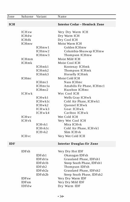
ICH Interior Cedar – Hemlock Zone
ICHxw Very Dry Warm ICHICHdw Dry Warm ICHICHdk Dry Cool ICHICHmw Moist Warm ICH
ICHmw1 Golden ICHmwICHmw2 Columbia-Shuswap ICHmwICHmw3 Thompson ICHmw
ICHmm Moist Mild ICHICHmk Moist Cool ICH
ICHmk1 Kootenay ICHmkICHmk2 Thompson ICHmkICHmk3 Horsefly ICHmk
ICHmc Moist Cold ICHICHmc1 Nass ICHmcICHmc1a Amabilis Fir Phase, ICHmc1ICHmc2 Hazelton ICHmc
ICHwk Wet Cool ICHICHwk1 Wells Gray ICHwkICHwk1c Cold Air Phase, ICHwk1ICHwk2 Quesnel ICHwkICHwk3 Goat ICHwkICHwk4 Cariboo ICHwk
ICHwc Wet Cold ICHICHvk Very Wet Cool ICH
ICHvk1 Mica ICHvkICHvk1c Cold Air Phase, ICHvk1ICHvk2 Slim ICHvk
ICHvc Very Wet Cold ICH
IDF Interior Douglas-fir Zone
IDFxh Very Dry Hot IDFIDFxh1 Okanagan IDFxhIDFxh1a Grassland Phase, IDFxh1IDFxh1b Steep South Phase, IDFxh1IDFxh2 Thompson IDFxhIDFxh2a Grassland Phase, IDFxh2IDFxh2b Steep South Phase, IDFxh2
IDFxw Very Dry Warm IDFIDFxm Very Dry Mild IDFIDFdw Dry Warm IDF
Zone Subzone Variant Name
•35•
Zone Subzone Variant Name
IDFdm Dry Mild IDFIDFdm1 Kettle IDFdmIDFdm2 Kootenay IDFdm
IDFdk Dry Cool IDFIDFdk1 Thompson IDFdkIDFdk1a Grassland Phase, IDFdk1IDFdk1b Steep South Phase, IDFdk1IDFdk2 Cascade IDFdkIDFdk2b Steep South Phase, IDFdk2IDFdk3 Fraser IDFdkIDFdk4 Chilcotin IDFdk
IDFmw Moist Warm IDFIDFmw1 Okanagan IDFmwIDFmw2 Thompson IDFmwIDFmw2a Grassland Phase, IDFmw2
IDFww Wet Warm IDF
MH Mountain Hemlock Zone
MHmm Moist Maritime MHMHmm1 Windward MHmmMHmm2 Leeward MHmmMHmm2e Engelmann Spruce Phase, MHmm2
MHwh Wet Hypermaritime MHMHwh1 Windward MHwhMHwh2 Leeward MHwh
MHmmp Moist Maritime Parkland MHMHmmp1 Windward MHmmpMHmmp2 Leeward MHmmpMHmmp2e Engelmann Spruce Phase, MHmmp2
MHwhp Wet Hypermaritime Parkland MHMHwhp1 Windward MHwhpMHwhp2 Leeward MHwhp
MS Montane Spruce Zone
MSxk Very Dry Cool MSMSxv Very Dry Very Cold MSMSdm Dry Mild MS
MSdm1 Okanagan MSdmMSdm2 Thompson MSdm
MSdk Dry Cool MSMSdc Dry Cold MS

•36•
MSdc1 Bridge MSdcMSdc2 Tatlayoko MSdc
MSdv Dry Very Cold MS
PP Ponderosa Pine Zone
PPxh Very Dry Hot PPPPxh1 Okanagan PPxhPPxh1a Grassland Phase, PPxh1PPxh2 Thompson PPxhPPxh2a Grassland Phase, PPxh2
PPdh Dry Hot PPPPdh1 Kettle PPdhPPdh2 Kootenay PPdh
SBPS Sub-Boreal Pine – Spruce Zone
SBPSxc Very Dry Cold SBPSSBPSdc Dry Cold SBPSSBPBmk Moist Cool SBPSSBPSmc Moist Cold SBPS
SBS Sub-Boreal Spruce Zone
SBSdh Dry Hot SBSSBSdh1 McLennan SBSdhSBSdh2 Robson SBSdh
SBSdw Dry Warm SBSSBSdw1 Horsefly SBSdwSBSdw2 Blackwater SBSdwSBSdw3 Stuart SBSdw
SBSdk Dry Cool SBSSBSmh Moist Hot SBSSBSmw Moist Warm SBSSBSmm Moist Mild SBSSBSmk Moist Cool SBS
SBSmk1 Mossvale SBSmkSBSmk2 Williston SBSmk
SBSmc Moist Cold SBSSBSmc1 Moffat SBSmcSBSmc2 Babine SBSmcSBSmc3 Kluskus SBSmc
Zone Subzone Variant Name

•37•
SBSwk Wet Cool SBSSBSwk1 Willow SBSwkSBSwk2 Finlay-Peace SBSwkSBSwk3 Takla SBSwkSBSwk3a Douglas-fir Phase, SBSwk3
SBSvk Very Wet Cool SBS
SWB Spruce – Willow – Birch Zone
SWBdk Dry Cool SWBSWBdks Dry Cool Scrub SWBSWBmk Moist Cool SWBSWBmks Moist Cool Scrub SWBSWBvk Very Wet Cool SWBSWBvks Very Wet Cool Scrub SWB
Zone Subzone Variant Name

•38•
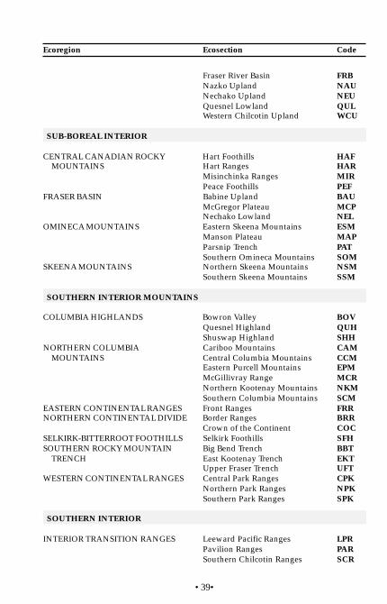
APPENDIX 1.2. Ecosections of British Columbia
Ecoregion Ecosection Code
COAST AND MOUNTAINS
CASCADE RANGES Northwestern Cascade Ranges NWCCASCADIA CONTINENTAL SHELF Vancouver Island Shelf VISCOASTAL GAP Hecate Lowland HEL
Kitimat Ranges KIRHECATE CONTINENTAL SHELF Dixon Entrance DIE
Hecate Strait HESQueen Charlotte Sound QCSQueen Charlotte Strait QCT
NASS BASIN NABNASS RANGES NARNORTHERN COASTAL MOUNTAINS Alaska Panhandle Mountains APM
Alsek Ranges ALRBoundary Ranges BOR
PACIFIC RANGES Eastern Pacific Ranges EPRNorthern Pacific Ranges NPROuter Fiordland OUFSouthern Pacific Ranges SPR
QUEEN CHARLOTTE LOWLAND QCLQUEEN CHARLOTTE RANGES Skidegate Plateau SKP
Windward Queen Charlotte Mtns. WQCWESTERN VANCOUVER ISLAND Nahwitti Lowland NWL
Northern Island Mountains NIMWindward Island Mountains WIM
GEORGIA DEPRESSION
EASTERN VANCOUVER ISLAND Leeward Island Mountains LIMNanaimo Lowland NAL
LOWER MAINLAND Fraser Lowland FRLGeorgia Lowland GEL
GEORGIA-PUGET BASIN Juan de Fuca Strait JDFSouthern Gulf Islands SGIStrait of Georgia SOG
CENTRAL INTERIOR
BULKLEY RANGES BURCHILCOTIN RANGES Central Chilcotin Ranges CCR
Western Chilcotin Ranges WCRFRASER PLATEAU Bulkley Basin BUB
Cariboo Basin CABCariboo Plateau CAPChilcotin Plateau CHP
•39•
Fraser River Basin FRBNazko Upland NAUNechako Upland NEUQuesnel Lowland QULWestern Chilcotin Upland WCU
SUB-BOREAL INTERIOR
CENTRAL CANADIAN ROCKY Hart Foothills HAFMOUNTAINS Hart Ranges HAR
Misinchinka Ranges MIRPeace Foothills PEF
FRASER BASIN Babine Upland BAUMcGregor Plateau MCPNechako Lowland NEL
OMINECA MOUNTAINS Eastern Skeena Mountains ESMManson Plateau MAPParsnip Trench PATSouthern Omineca Mountains SOM
SKEENA MOUNTAINS Northern Skeena Mountains NSMSouthern Skeena Mountains SSM
SOUTHERN INTERIOR MOUNTAINS
COLUMBIA HIGHLANDS Bowron Valley BOVQuesnel Highland QUHShuswap Highland SHH
NORTHERN COLUMBIA Cariboo Mountains CAMMOUNTAINS Central Columbia Mountains CCM
Eastern Purcell Mountains EPMMcGillivray Range MCRNorthern Kootenay Mountains NKMSouthern Columbia Mountains SCM
EASTERN CONTINENTAL RANGES Front Ranges FRRNORTHERN CONTINENTAL DIVIDE Border Ranges BRR
Crown of the Continent COCSELKIRK-BITTERROOT FOOTHILLS Selkirk Foothills SFHSOUTHERN ROCKY MOUNTAIN Big Bend Trench BBT
TRENCH East Kootenay Trench EKTUpper Fraser Trench UFT
WESTERN CONTINENTAL RANGES Central Park Ranges CPKNorthern Park Ranges NPKSouthern Park Ranges SPK
SOUTHERN INTERIOR
INTERIOR TRANSITION RANGES Leeward Pacific Ranges LPRPavilion Ranges PARSouthern Chilcotin Ranges SCR
Ecoregion Ecosection Code

•40•
OKANOGAN HIGHLAND Southern Okanogan Basin SOBSouthern Okanogan Highland SOH
NORTHERN CASCADE RANGES Hozameen Range HOROkanagan Range OKR
THOMPSON-OKANAGAN PLATEAU Northern Okanagan Basin NOBNorthern Okanagan Highland NOHNorthern Thompson Upland NTUSouthern Thompson Upland STUThompson Basin THB
BOREAL PLAINS
CENTRAL ALBERTA UPLAND Clear Hills CLHHalfway Plateau HAP
SOUTHERN ALBERTA UPLAND Kiskatinaw Plateau KIPPEACE RIVER BASIN Peace Lowland PEL
TAIGA PLAINS
HAY RIVER LOWLAND Fort Nelson Lowland FNLMUSKWA PLATEAU MUPNORTHERN ALBERTA UPLAND Etsho Plateau ETP
Maxhamish Upland MAUPetitot Plain PEP
NORTHERN BOREAL MOUNTAINS
HYLAND HIGHLAND HYHLIARD BASIN Liard Plain LIPNORTHERN CANADIAN ROCKY Eastern Muskwa Ranges EMR
MOUNTAINS Muskwa Foothills MUFWestern Muskwa Ranges WMR
BOREAL MOUNTAINS AND Cassiar Ranges CARPLATEAUS Kechika Mountains KEM
Southern Boreal Plateau SBPStikine Plateau STPTeslin Plateau TEPTuya Range TUR
SOUTHERN YUKON LAKES Teslin Basin TEBST. ELIAS MOUNTAINS Icefield Ranges ICRYUKON-STIKINE HIGHLANDS Tagish Highland TAH
Tahltan Highland THHTatshenshini Basin TAB
Ecoregion Ecosection Code

•1•
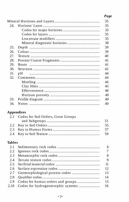
Contents
Soil Description Form ............................................................... 4Field Procedure .......................................................................... 5Completing the Form ............................................................... 6
1. Surveyor .......................................................................... 62. Plot No. ........................................................................... 63. Bedrock Type .................................................................. 64. Coarse Fragment Lithology ......................................... 85. Terrain Classification .................................................... 86. Soil Classification .......................................................... 147. Humus Form .................................................................. 158. Hydrogeomorphic Units .............................................. 159. Rooting Depth ................................................................ 18
10. Rooting Zone Particle-Size ........................................... 1811. Root Restricting Layer .................................................. 2012. Water source ................................................................... 2013. Seepage Water Depth .................................................... 2114. Drainage Class and Soil Moisture Subclass ............... 2115. Flooding Regime ............................................................ 23
Organic Horizons and Layers ................................................. 2416. Horizon/Layer ............................................................... 24
Codes for master organic horizons ......................... 25Codes for subordinate organic horizons ................ 25Lowercase modifiers ................................................. 26Codes for organic layers ........................................... 27Tiers ............................................................................. 27
17. Depth .............................................................................. 2718. Fabric .............................................................................. 28
Structure ...................................................................... 28von Post scale of decomposition ............................. 29
19. Mycelial Abundance ..................................................... 3020. Fecal Abundance............................................................ 3021. Roots .............................................................................. 3122. pH .............................................................................. 3123. Comments section ......................................................... 32
Consistence ................................................................. 32Character .................................................................... 32
2 SOIL DESCRIPTION
Page
•2•
Mineral Horizons and Layers .................................................. 3524. Horizon/Layer ............................................................... 35
Codes for major horizons ......................................... 35Codes for layers ......................................................... 35Lowercase modifiers ................................................. 35Mineral diagnostic horizons .................................... 38
25. Depth .............................................................................. 3926. Colour .............................................................................. 3927. Texture ............................................................................. 4028. Percent Coarse Fragments ............................................ 4129. Roots .............................................................................. 4130. Structure .......................................................................... 4231. pH .............................................................................. 4432. Comments ....................................................................... 44
Mottling ...................................................................... 44Clay films.................................................................... 45Effervescence .............................................................. 48Horizon porosity ....................................................... 49
33. Profile diagram .............................................................. 4934. Notes .............................................................................. 49
Appendices2.1 Codes for Soil Orders, Great Groups
and Subgroups ........................................................... 512.2 Key to Soil Orders .......................................................... 552.3 Key to Humus Forms .................................................... 572.4 Key to Soil Texture ......................................................... 59
Tables2.1 Sedimentary rock codes ............................................... 62.2 Igneous rock codes ........................................................ 72.3 Metamorphic rock codes .............................................. 82.4 Terrain texture codes ..................................................... 92.5 Surficial material codes ................................................. 112.6 Surface expression codes .............................................. 122.7 Geomorphological process codes ............................... 132.8 Qualifier codes ................................................................ 142.9 Codes for humus orders and groups ......................... 15
2.10 Codes for hydrogeomorphic systems ....................... 16
Page
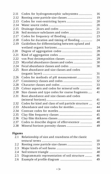
•3•
2.11 Codes for hydrogeomorphic subsystems ................. 162.12 Rooting zone particle size classes ................................ 192.13 Codes for root-restricting layers ................................. 202.14 Water source codes ........................................................ 202.15 Drainage classes and codes .......................................... 212.16 Soil moisture subclasses and codes ............................. 232.17 Codes for frequency of flooding ................................. 232.18 Codes for duration and timing of flooding ............... 242.19 Guidelines for differentiating between upland and
wetland organic horizons ............................................. 242.20 Degree of aggregation codes ....................................... 282.21 Kind of aggregation codes ........................................... 282.22 von Post decomposition classes .................................. 292.23 Mycelial abundance classes and codes ........................ 302.24 Fecal abundance classes and codes ............................. 302.25 Root abundance and size classes and codes
(organic layer) ................................................................ 312.26 Codes for methods of pH measurement ................... 312.27 Consistency classes and codes ..................................... 322.28 Character classes and codes ......................................... 332.29 Colour aspects and codes for mineral soils ............... 402.30 Size classes and type codes for coarse fragments ..... 412.31 Root abundance and size classes and codes
(mineral horizon) ........................................................... 412.32 Codes for kind and class of soil particle structure .... 422.33 Abundance and size codes for mottles ....................... 442.34 Contrast codes for mottles ........................................... 442.35 Clay film frequency classes .......................................... 452.36 Clay film thickness classes ............................................ 482.37 Codes to describe degree of effervescence ............... 482.38 Mineral horizon porosity classes ................................. 49
Figures2.1 Relationship of size and roundness of the clastic
textural terms ................................................................. 102.2 Rooting zone particle size classes ................................ 192.3 Major kinds of soil fauna .............................................. 342.4 Soil texture triangle ....................................................... 402.5 Diagrammatic representation of soil structure ......... 462.6 Example of profile diagram ......................................... 49

•4•
FAB
RIC
1
211
1G
EO
MO
RP
H.
PR
OC
ES
S
DE
PTH
ST
RU
CT
UR
EvP
OS
TM
YC
EL.
AB
.F
EC
AL
AB
.R
OO
TS
AB
.S
IZE
CO
MM
EN
TS
(co
nsis
tenc
y, c
hara
cter
, fau
na,
etc)
:
DE
PTH
CO
LOU
RA
SP.
TEXT
.H
OR
/L
AYE
R
OR
GA
NIC
HO
RIZ
ON
S/L
AY
ER
S
MIN
ER
AL
HO
RIZ
ON
S/L
AY
ER
S%
CO
AR
SE
FR
AG
ME
NT
SC
ST
OTA
LG
RO
OT
SA
B.
SIZ
ESH
APE
CLA
SS
KIN
DS
TR
UC
TU
RE
GE
OLO
GY
BE
DR
OC
K
SO
IL C
LAS
S.
TE
XT
UR
E
cmcm
RO
OT
ING
DE
PT
HR
OO
TR
ES
TR
ICT.
LAY
ER
TY
PE
DE
PT
H
WAT
ER
SO
UR
CE
SE
EPA
GE
DR
AIN
AG
E
FLO
OD
RG
.
TE
RR
AIN
2
NO
TE
S:
HO
R/
LAY
ER
pH
SOIL DESCRIPTION
R. Z
. PA
RT.
SIZ
E
cm
C. F
. LIT
H.
SU
RV
EYO
R(S
)
pHC
OM
ME
NT
S (
mot
tles,
cla
y fil
ms,
effe
rves
c., e
tc):
PLO
T N
O.
SU
RF
ICIA
LM
ATE
RIA
LS
UR
FAC
EE
XP
R.
22
PR
OF
ILE
DIA
GR
AM
HU
MU
S F
OR
MH
YD
RO
GE
O.
FS
882
(2)
HR
E 9
8/5
3322
32318
1
1213 23
3029
2827
1920
2122
11
7
43
5
69
10
1817
16 2425
26
3451134
14
15

•5•
Field Procedure
Getting Started1. Locate plot boundaries, assess variability, select pit location(s).2. Excavate pit (generally 50–75 cm in depth) leaving the face and sides
undisturbed around the ground surface.3. While excavating, observe:
• organic horizon depths and fabric;• mineral horizon depths, colours, structure, and textural changes;• percentage and shape of coarse fragments;• rooting abundance, depth, and restrictions; and• mottling, water seepage, or water table.
4. Lay out notes, forms, and soil description tools.5. Clean off face from top to bottom (and photograph if required).
• Note horizon changes and mark with knife indentations or golf tees.• Collect soil texture samples from bottom to top and put aside.
Record and Classify (see tab numbers on sample f orm, facing page)Designate horizons on form (organic and mineral horizons/layers).For each horizon (depending on survey objectives/requirements):• Record average starting and ending depths.• For organic horizon, record fabric, mycelia and fecal abundance, rooting,
and pH.• For mineral horizons, hand-texture soil samples and determine colours.
Record percent and shape of coarse fragments, rooting, structure, and pH.• Note important observations in comments (e.g. soil fauna, mottles, clay
films, etc.).• confirm original horizon designationsSketch a profile diagram to approximate scale.
Record:• rooting depth, particle size, and restricting layer• water source, seepage depth, drainage class, and flooding regimeClassify:• bedrock geology and coarse fragment lithology type(s)• terrain unit(s), soil pedon, humus form, and hydrogeomorphic unitUse the “Notes” section to summarize or describe important soil featuresnot otherwise collected on the form, or are significant to the study, classifica-tions, or management interpretations.
Check and IntegrateCheck the form to ensure there are no missing data, and then (under mostcircumstances) fill in the pit. Strike through any fields that were not assessed.Integrate the soil data with other site factors to determine and record the soilmoisture and soil nutrient regimes on the site description form.
2
1
3
4
5
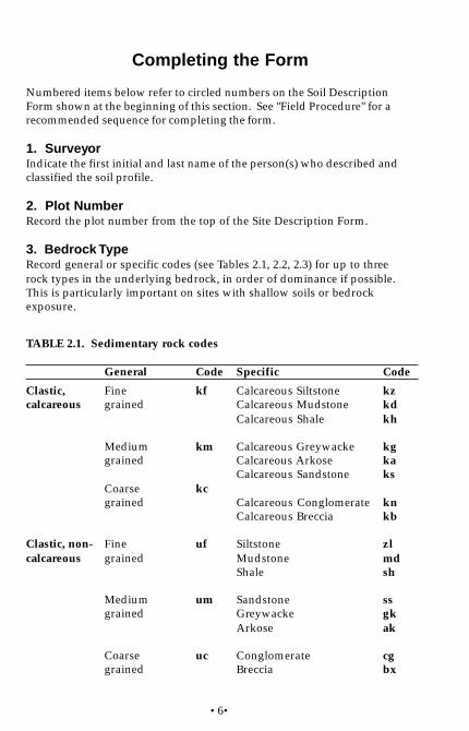
•6•
Completing the Form
Numbered items below refer to circled numbers on the Soil DescriptionForm shown at the beginning of this section. See "Field Procedure" for arecommended sequence for completing the form.
1. SurveyorIndicate the first initial and last name of the person(s) who described andclassified the soil profile.
2. Plot NumberRecord the plot number from the top of the Site Description Form.
3. Bedrock TypeRecord general or specific codes (see Tables 2.1, 2.2, 2.3) for up to threerock types in the underlying bedrock, in order of dominance if possible.This is particularly important on sites with shallow soils or bedrockexposure.
TABLE 2.1. Sedimentary rock codes
Clastic,calcareous
Clastic, non-calcareous
General
Finegrained
Mediumgrained
Coarsegrained
Finegrained
Mediumgrained
Coarsegrained
Code
kf
km
kc
uf
um
uc
Specific
Calcareous SiltstoneCalcareous MudstoneCalcareous Shale
Calcareous GreywackeCalcareous ArkoseCalcareous Sandstone
Calcareous ConglomerateCalcareous Breccia
SiltstoneMudstoneShale
SandstoneGreywackeArkose
ConglomerateBreccia
Code
kzkdkh
kgkaks
knkb
zlmdsh
ssgkak
cgbx

•7•
TABLE 2.2. Igneous rock codes
Precipitates,crystalline
Organic
General
Calcareous
Non-calcareous
Calcareous
Carbonaceous
Code
pk
pu
ok
oc
Specific
TravertineLimestoneDolomite
GypsumLimoniteBarite
Mar
LigniteCoal
Code
tvlsdo
gyliba
ma
lgco
Intrusive
Extrusive
GeneralAcid (felsic)
Intermediate
Basic (mafic)
Acid (felsic)
Intermediate
Basic (mafic)
Recent lava flow
Pyroclastic
Codeia
ii
ib
ea
ei
eb
la
ep
SpecificSyeniteGraniteQuartz MonzoniteGranodiorite
Quartz DioriteDiorite
QuartzGabbroPyroxeniteDunite
TrachyteRhyoliteDacite
Andesite
Quartz BasaltBasalt
TuffVolcanic BrecciaAgglomerate
Codesygrqmgd
qddi
qggbpydu
trrhda
an
qbbs
tuvbag

•8•
TABLE 2.3. Metamorphic rock codes
4. Coarse Fragment LithologyRecord up to three rock types in order of dominance from left to right onthe form that make up the coarse fraction (i.e., gravels, cobbles, and stones)of the soil material. Characters are recorded using the same codes asoutlined for bedrock type. If the lithologies are so mixed that dominancecan not be determined, record by entering the code “mx.”
5. Terrain ClassificationFour information fields are provided for recording terrain texture, surficialmaterial, surface expression and geomorphological process, respectively(Howes and Kenk 1997) (see Tables 2.4, 2.5, 2.6, and 2.7 and Figure 2.1). Upto three codes can be entered in each of these fields. Place qualifyingdescriptor codes (Table 2.8) in the appropriate field to the right of any othercodes used in that field (superscript codes are no longer used). Code line 1for the uppermost stratigraphic layer, and code line 2 for an underlyinglayer. For those wishing to use terrain subclasses and subtypes, refer toHowes and Kenk (1997).
Foliated
Non-foliated
General
Fine grained
Medium tocoarse grained
Coarse grained
Fine grained
Medium tocoarse grained
Coarse grained
Calcareous
Code
ff
fm
fc
nf
nm
nc
nk
Specific
SlatePhylite
SchistGneissGranite GneissDiorite Gneiss
Migmatite
ArgilliteSerpentinite
QuartziteHornfelsGranulite
AmphiboliteHornblendite
MarbleDolomite MarbleSerpentine Marble
Code
slph
scgnggdg
mi
arsp
qthfgl
amhb
mbdmsm
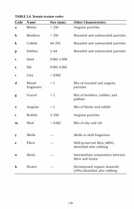
•9•
TABLE 2.4. Terrain texture codes
Code Name Size (mm) Other Characteristics
a Blocks > 256 Angular particles
b Boulders > 256 Rounded and subrounded particles
k Cobble 64–256 Rounded and subrounded particles
p Pebbles 2–64 Rounded and subrounded particles
s Sand 0.062–2.000
z Silt 0.002–0.062
c Clay < 0.002
d Mixed > 2 Mix of rounded and angularfragments particles
g Gravel > 2 Mix of boulders, cobbles, andpebbles
x Angular > 2 Mix of blocks and rubble
r Rubble 2–256 Angular particles
m Mud < 0.062 Mix of clay and silt
y Shells — Shells or shell fragments
e Fibric — Well-preserved fibre; (40%)identified after rubbing
u Mesic — Intermediate composition betweenfibric and humic
h Humic — Decomposed organic material;(10%) identified after rubbing
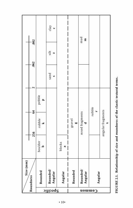
•10•
Siz
e (m
m)
Rou
nd
nes
s2
6425
6.0
62.0
02
Specific Common
Rou
nd
ed
Rou
nd
ed/
An
gula
r
An
gula
r
Rou
nd
ed
Rou
nd
ed/
An
gula
r
An
gula
r
boul
der
bco
bble
kpe
bble
p
sand s
silt z
clay c
bloc
ksa
grav
elg
mxe
d fr
agm
ents
d
rubb
ler
angu
lar f
ragm
ents
x
mud m
FIG
UR
E 2
.1.
Rel
atio
nsh
ip o
f si
ze a
nd
rou
nd
nes
s of
th
e cl
asti
c te
xtu
ral
term
s.

•11•
TABLE 2.5. Surficial (genetic) material codes
Code Name (Assumed Descriptionstatus)
A Anthropogenic (A) Artificial or human-modified material
C Colluvium (A) Products of mass wastage
D Weathered bedrock (A) In situ, decomposedbedrock
E Eolian (I) Materials deposited bywind action
F Fluvial (I) River deposits
FG Glaciofluvial (I) Ice contact fluvial material
I Ice (A) Permanent snow, glaciers,and icefields
L Lacustrine (I) Lake sediments; includeswave deposits
LG Glaciolacustrine (I) Ice contact lacustrinematerial
M Morainal (I) Material deposited directlyby glaciers
O Organic (A) Accumulation/decay ofvegetative matter
R Bedrock (–) Outcrops/rocks covered byless than 10 cm of soil
U Undifferentiated (–) Layered sequence; threematerials or more
V Volcanic (I) Unconsolidated pyroclasticsediments
W Marine (I) Marine sediments; includeswave deposits
WG Glaciomarine (I) Ice contact marinesediments
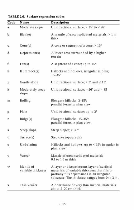
•12•
TABLE 2.6. Surface expression codes
Code Name Descriptiona Moderate slope Unidirectional surface; > 15° to < 26°
b Blanket A mantle of unconsolidated materials; > 1 mthick
c Cone(s) A cone or segment of a cone; > 15°
d Depression(s) A lower area surrounded by a higherterrain
f Fan(s) A segment of a cone; up to 15°
h Hummock(s) Hillocks and hollows, irregular in plan;15–35°
j Gentle slope Unidirectional surface; > 3° and < 15°
k Moderately steep Unidirectional surface; > 26° and < 35slope
m Rolling Elongate hillocks; 3–15°;parallel forms in plan view
p Plain Unidirectional surface; up to 3°
r Ridge(s) Elongate hillocks; 15–35°;parallel forms in plan view
s Steep slope Steep slopes; > 35°
t Terrace(s) Step-like topography
u Undulating Hillocks and hollows; up to < 15°; irregular inplan view
v Veneer Mantle of unconsolidated material;0.1 to 1.0 m thick
w Mantle of A layer or discontinuous layer of surficialvariable thickness materials of variable thickness that fills or
partially fills depressions in an irregularsubstrate. The thickness ranges from 0 to 3 m.
x Thin veneer A dominance of very thin surficial materialsabout 2–20 cm thick
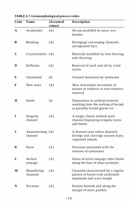
•13•
TABLE 2.7. Geomorphological process codes
Code Name (Assumed Descriptionstatus)
A Avalanches (A) Terrain modified by snow ava-lanches
B Braiding (A) Diverging/converging channels;unvegetated bars
C Cryoturbation (A) Materials modified by frost heavingand churning
D Deflation (A) Removal of sand and silt by windaction
E Channeled (I) Channel formation by meltwater
F Slow mass (A) Slow downslope movement ofmasses of cohesive or non-cohesivematerial
H Kettle (I) Depressions in surficial materialresulting from the melting of buriedor partially buried glacier ice
I Irregular (A) A single, clearly defined mainchannel channel displaying irregular turns
and bends
J Anastomosing (A) A channel zone where channelschannel diverge and converge around many
vegetated islands
K Karst (A) Processes associated with thesolution of carbonates
L Surface (A) Zones of active seepage often foundseepage along the base of slope positions
M Meandering (A) Channels characterized by a regularchannels pattern of bends with uniformed
amplitude and wave length
N Nivation (A) Erosion beneath and along themargin of snow patches
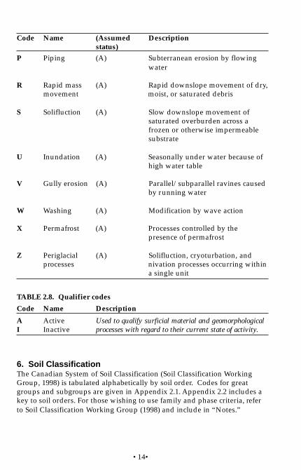
•14•
TABLE 2.8. Qualifier codes
6. Soil ClassificationThe Canadian System of Soil Classification (Soil Classification WorkingGroup, 1998) is tabulated alphabetically by soil order. Codes for greatgroups and subgroups are given in Appendix 2.1. Appendix 2.2 includes akey to soil orders. For those wishing to use family and phase criteria, referto Soil Classification Working Group (1998) and include in “Notes.”
Code Name (Assumed Descriptionstatus)
P Piping (A) Subterranean erosion by flowingwater
R Rapid mass (A) Rapid downslope movement of dry,movement moist, or saturated debris
S Solifluction (A) Slow downslope movement ofsaturated overburden across afrozen or otherwise impermeablesubstrate
U Inundation (A) Seasonally under water because ofhigh water table
V Gully erosion (A) Parallel/subparallel ravines causedby running water
W Washing (A) Modification by wave action
X Permafrost (A) Processes controlled by thepresence of permafrost
Z Periglacial (A) Solifluction, cryoturbation, andprocesses nivation processes occurring within
a single unit
Code Name Description
A Active Used to qualify surficial material and geomorphologicalI Inactive processes with regard to their current state of activity.
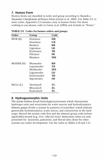
•15•
7. Humus FormHumus forms are classified to order and group according to Towards aTaxonomic Classification of Humus Forms (Green et al. 1993) Use Table 2.9 toenter codes. Appendix 2.3 contains a key to humus forms. For thosewishing to use phases, refer to Green et.al. (1993), and include in “Notes.”
TABLE 2.9. Codes for humus orders and groups
Order Group Code
MOR (R) Hemimor HRHumimor URResimor RRLignomor LRHydromor YRFibrimor FRMesimor MR
MODER (D) Mormoder RDLeptomoder TDMullmoder MDLignomoder LDHydromoder YDSaprimoder SD
MULL (L) Vermimull VLRhizomull ZLHydromull YL
8. Hydrogeomorphic UnitsThe system defines broad hydrological processes which characterizelandscape units and ecosystems by water sources and hydrodynamics.Element groups divide a system by patterns of waterflow which indicategenerically hydrodynamics, water source, and connectivity in the land-scape. Record the system code first and the element group code (whereapplicable) second (e.g., Fra= alluvial river). Subsystem codes are onlypresented for lacustrine, palustrine, and fluvial sites; those for othersystems are under development. Use the codes in Tables 2.10 and 2.11.
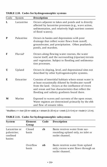
•16•
a Modifiers: r = river (20 m+ wide); s = stream (5–20 m); c = creek (1.5–5 m); v = rivulet (< 1.5 m).
TABLE 2.10. Codes for hydrogeomorphic systems
TABLE 2.11. Codes for hydrogeomorphic subsystems
Description
Occurs adjacent to lakes and ponds and is directlyaffected by lacustrine processes (e.g., wave action,sedimentation, and relatively high nutrient contentof flood waters).
Occurs in basins and depressions with poordrainage that collect water flows from runoff,groundwater, and precipitation. Often peatlands,ponds, and marshes.
Occurs along flowing water courses, the watercourse itself, and the surrounding (riparian) terrainand vegetation. Subject to flooding and sedimenta-tion processes.
Occurs in sloping, level, and depressional sites notdescribed by other hydrogeomorphic systems.
Consists of intertidal habitats where ocean water isat least occasionally diluted by freshwater runofffrom the land. Occurs at the confluence of riversand ocean and has characteristics that reflect theflooding and salinity gradients found there.
Exposed to waves and currents of the open ocean.Water regimes are determined primarily by the ebband flow of oceanic tides.
Code System
L Lacustrine
P Palustrine
F Fluviala
U Upland
E Estuarine
M Marine
Description
Basin receives water from sur-rounding upland only, no inlet oroutlet channel.
Basin receives water from uplandonly; excess water flows through anoutlet channel.
System
Lacustrine orpalustrine;confinedbasins
ElementGroup
Closedbasin
Overflowbasin
Code
cb
ob
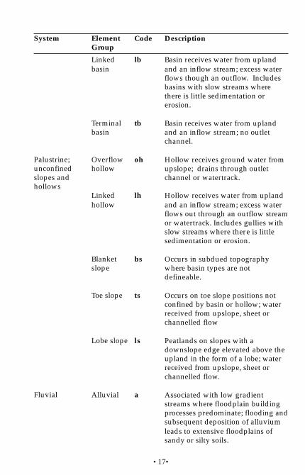
•17•
System
Palustrine;unconfinedslopes andhollows
Fluvial
ElementGroup
Linkedbasin
Terminalbasin
Overflowhollow
Linkedhollow
Blanketslope
Toe slope
Lobe slope
Alluvial
Code
lb
tb
oh
lh
bs
ts
ls
a
Description
Basin receives water from uplandand an inflow stream; excess waterflows though an outflow. Includesbasins with slow streams wherethere is little sedimentation orerosion.
Basin receives water from uplandand an inflow stream; no outletchannel.
Hollow receives ground water fromupslope; drains through outletchannel or watertrack.
Hollow receives water from uplandand an inflow stream; excess waterflows out through an outflow streamor watertrack. Includes gullies withslow streams where there is littlesedimentation or erosion.
Occurs in subdued topographywhere basin types are notdefineable.
Occurs on toe slope positions notconfined by basin or hollow; waterreceived from upslope, sheet orchannelled flow
Peatlands on slopes with adownslope edge elevated above theupland in the form of a lobe; waterreceived from upslope, sheet orchannelled flow.
Associated with low gradientstreams where floodplain buildingprocesses predominate; flooding andsubsequent deposition of alluviumleads to extensive floodplains ofsandy or silty soils.

•18•
9. Rooting DepthRooting depth refers to the depth (cm) from the ground surface, which is thetop of the uppermost soil horizon including organic horizons (e.g., Fm1),down to the bottom of the rooting zone (i.e., the level at which the majorityof roots stop; for example, the end of “plentiful” and beginning of “few”rooting abundance).
10. Rooting Zone Particle SizeThe particle size distribution within the mineral portion of the rooting zoneis used to make broad interpretations. After determining rooting depth,estimate the rooting zone particle-size class as a weighted average of themineral horizons within the rooting zone (Figure 2.2, Table 2.12). Whererooting is restricted to the organic horizons, use the organic material codesin Table 2.12. For the most part, class names and definitions have beenmodified from the Canadian System of Soil Classification family particlesize criteria. Rooting zone classes are greatly simplified and use onlypercent coarse fragments(> 2 mm) by volume, and texture class sizes by percent weight for sand(.05 to < 2 mm), silt (< .05 to .002 mm), and clay (< .002). Two differentclasses can be entered on the data form if strongly contrasting size classesoccur (e.g. CLS/FC= coarse-loamy over fine-clayey), however ranges ofrooting zone particle-size classes can not be shown.
ElementGroup
Transport
Headwater
Code
t
h
Description
Associated with moderate gradientstreams where neither erosion ordeposition forces predominate;floodplain development limited, in-stream bars and gravelly soilcommon.
Associated with high gradientstreams where erosive processespredominate; flood plain and bardevelopment limited; cobble, stoneor bedrock substrates common
System
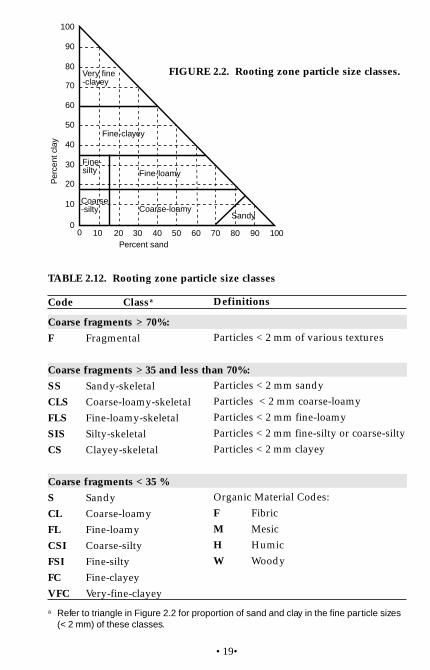
•19•
Code Classa
Coarse fragments > 70%:
F Fragmental
Coarse fragments > 35 and less than 70%:
SS Sandy-skeletalCLS Coarse-loamy-skeletalFLS Fine-loamy-skeletalSIS Silty-skeletalCS Clayey-skeletal
Coarse fragments < 35 %
S SandyCL Coarse-loamyFL Fine-loamyCSI Coarse-siltyFSI Fine-siltyFC Fine-clayeyVFC Very-fine-clayey
Definitions
Particles < 2 mm of various textures
Particles < 2 mm sandyParticles < 2 mm coarse-loamyParticles < 2 mm fine-loamyParticles < 2 mm fine-silty or coarse-siltyParticles < 2 mm clayey
Organic Material Codes:F FibricM MesicH HumicW Woody
a Refer to triangle in Figure 2.2 for proportion of sand and clay in the fine particle sizes(< 2 mm) of these classes.
00
10 20 30 40 50 60 70 80 90 100
10
20
30
40
50
60
70
80
90
100
Percent sand
Per
cent
cla
y
Coarse-loamySandy
Coarse-silty
Fine-silty Fine-loamy
Fine-clayey
Very fine-clayey
FIGURE 2.2. Rooting zone particle size classes.
TABLE 2.12. Rooting zone particle size classes

•20•
12. Water SourceThe most influential source of water on a site (determined by a qualitativeassessment) is recorded using the codes in Table 2.14.
TABLE 2.13. Codes for root restricting layers
TABLE 2.14. Water source codes
Code DescriptionC Strongly cemented horizon
P Clay pan or restriction due to fines
K Compacted morainal material
L Lithic contact
W Excessive moisture; this refers to the depth where the roots arebeing restricted by excessive moisture, but does not require thepresence of free water at the time of sampling
X Excessive accumulations of chemicals within the profile whichinhibit root growth (i.e., CaCO3 )
Z Permafrost; characterized by temperatures never exceeding 0°C,ice cementation, ice lenses, or massive ice.
N No root restriction evident.
11. Root Restricting LayerIf present, enter a code for the type of root restricting layer (Table 2.13), andthe depth (cm) from the ground surface down to the top of the layer.
Code Water Source
P Precipitation
G Groundwater
S Snowmelt (prolonged through the growing season)
F Stream sub-irrigation and flooding
M Mineral spring
T Tidal, freshwater
E Tidal, saltwater
Z Permafrost

•21•
13. Seepage Water DepthIf seepage is present at the time of sampling, record the depth (cm) from theground surface to the level of temporary or permanent subsurface waterflow. Enter “NP” if not present.
14. Drainage Class and Soil Moisture SubclassDrainage class describes the speed and extent to which water is removedfrom a mineral soil in relation to additions (Table 2.15.) s
TABLE 2.15. Drainage classes and codes
Description
Water is removed from the soil very rapidly inrelation to supply. Water source is precipitationand available water storage capacity followingprecipitation is essentially nil. Soils are typicallyfragmental or skeletal, shallow, or both.
Water is removed from the soil rapidly inrelation to supply. Excess water flows down-ward if underlying material is pervious.Subsurface flow may occur on steep gradientsduring heavy rainfall. Water source is precipita-tion. Soils are generally coarse textured.
Water is removed from the soil readily, but notrapidly. Excess water flows downward readilyinto underlying pervious material or laterally assubsurface flow. Water source is precipitation.On slopes, subsurface flow may occur for shortdurations, but additions are equalled by losses.Soils are generally intermediate in texture andlack restricting layers.
Water is removed from the soil somewhatslowly in relation to supply because of impervi-ousness or lack of gradient. Precipitation is thedominant water source in medium- to fine-textured soils; precipitation and significantadditions by subsurface flow are necessary incoarse-textured soils.
Code Class
x Very rapidlydrained
r Rapidly drained
w Well drained
m Moderatelywell drained

•22•
Code Class
i Imperfectlydrained
p Poorly drained
v Very poorlydrained
Description
Water is removed from the soil sufficientlyslowly in relation to supply to keep the soil wetfor a significant part of the growing season.Excess water moves slowly downward ifprecipitation is the major source. If subsurfacewater or groundwater (or both) is the mainsource, the flow rate may vary but the soilremains wet for a significant part of thegrowing season. Precipitation is the mainsource if available water storage capacity ishigh; contribution by subsurface orgroundwater flow (or both) increases asavailable water storage capacity decreases. Soilsgenerally have a wide range of texture, andsome mottling is common.
Water is removed so slowly in relation tosupply that the soil remains wet for much of thetime that it is not frozen. Excess water isevident in the soil for a large part of the time.Subsurface or groundwater flow (or both), inaddition to precipitation, are the main watersources. A perched water table may be present.Soils are generally mottled and/or gleyed.
Water is removed from the soil so slowly thatthe water table remains at or near the surfacefor most of the time the soil is not frozen.Groundwater flow and subsurface flow are themajor water sources. Precipitation is lessimportant, except where there is a perchedwater table with precipitation exceedingevapotranspiration. Typically associated withwetlands. For organic wetlands, also evaluatethe soil moisture subclass, and when enteringon the form, separate from drainage by a slash.For example, v/ac.
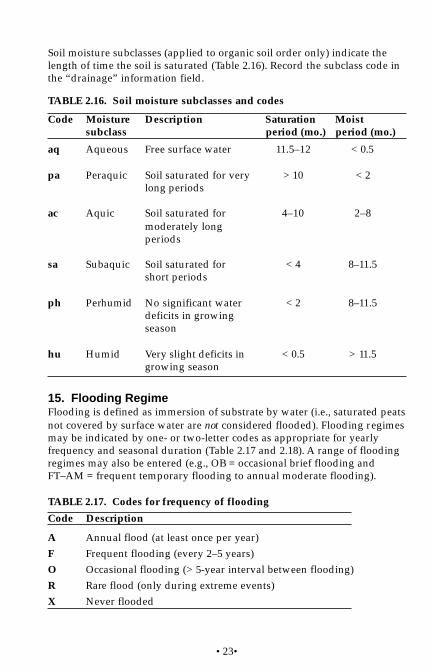
•23•
Soil moisture subclasses (applied to organic soil order only) indicate thelength of time the soil is saturated (Table 2.16). Record the subclass code inthe “drainage” information field.
15. Flooding RegimeFlooding is defined as immersion of substrate by water (i.e., saturated peatsnot covered by surface water are not considered flooded). Flooding regimesmay be indicated by one- or two-letter codes as appropriate for yearlyfrequency and seasonal duration (Table 2.17 and 2.18). A range of floodingregimes may also be entered (e.g., OB = occasional brief flooding andFT–AM = frequent temporary flooding to annual moderate flooding).
TABLE 2.17. Codes for frequency of flooding
TABLE 2.16. Soil moisture subclasses and codes
Code Moisturesubclass
aq Aqueous
pa Peraquic
ac Aquic
sa Subaquic
ph Perhumid
hu Humid
Description
Free surface water
Soil saturated for verylong periods
Soil saturated formoderately longperiods
Soil saturated forshort periods
No significant waterdeficits in growingseason
Very slight deficits ingrowing season
Code Description
A Annual flood (at least once per year)F Frequent flooding (every 2–5 years)O Occasional flooding (> 5-year interval between flooding)R Rare flood (only during extreme events)X Never flooded
Saturation period (mo.)
11.5–12
> 10
4–10
< 4
< 2
< 0.5
Moist period (mo.)
< 0.5
< 2
2–8
8–11.5
8–11.5
> 11.5
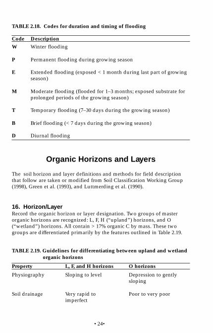
•24•
Organic Horizons and Layers
The soil horizon and layer definitions and methods for field descriptionthat follow are taken or modified from Soil Classification Working Group(1998), Green et al. (1993), and Luttmerding et al. (1990).
16. Horizon/LayerRecord the organic horizon or layer designation. Two groups of masterorganic horizons are recognized: L, F, H (“upland”) horizons, and O(“wetland”) horizons. All contain > 17% organic C by mass. These twogroups are differentiated primarily by the features outlined in Table 2.19.
TABLE 2.18. Codes for duration and timing of flooding
TABLE 2.19. Guidelines for differentiating between upland and wetlandorganic horizons
Code Description
W Winter flooding
P Permanent flooding during growing season
E Extended flooding (exposed < 1 month during last part of growingseason)
M Moderate flooding (flooded for 1–3 months; exposed substrate forprolonged periods of the growing season)
T Temporary flooding (7–30 days during the growing season)
B Brief flooding (< 7 days during the growing season)
D Diurnal flooding
Property
Physiography
Soil drainage
L, F, and H horizons
Sloping to level
Very rapid toimperfect
O horizons
Depression to gentlysloping
Poor to very poor

•25•
Codes for master organic horizons:L An upland horizon consisting of relatively fresh organic residues
that are readily identifiable as to origin.
F An upland horizon comprised of partly decomposed plant residuesin which fragmented plant structures are generally recognizable asto origin.
H An upland horizon comprised of well-decomposed plant residues inwhich plant structures are generally not recognizable.
O A wetland organic horizon comprised of materials in varying degreesof decomposition.
Property
Water table
Origin ofmaterials
L, F, and H horizons
Absent in organichorizons (may fluctuatein response to waterinput)
Organic residues fromplant communitiestypically associatedwith soil moistureregimes 0–6
O horizons
At or near ground surfacefor significant durationduring the frost-freeperiod
Organic residues fromplant communitiestypically associated withsoil moisture regimes 7–8
Codes for subordinate organic horizons:Ln An L horizon composed of newly accreted and essentially
unfragmented plant residues.
Lv An L horizon exhibiting initial decay and strong discoloration.
Fm An F horizon in which plant residues are aggregated in a mattedstructure, with a tenacious consistence. Fungal mycelia are clearly apredominant biotic component; some faunal droppings may bepresent.
Fz An F horizon in which plant residues are weakly aggregated with aloose or friable consistence. Faunal droppings are typically numer-ous and easily observed under magnification with a hand lens orbinocular microscope; fungal mycelia may be present.

•26•
Fa An F horizon in which plant residues are aggregated into a weak tomoderate, non-compact matted structure. This is an intergradebetween the Fm and Fz horizons, and as such, reflects properties ofboth, but neither fungal mycelia or faunal droppings predominates.
Hh An H horizon dominated by fine substances with very few, if any,recognizable plant residues.
Hz An H horizon dominated by fine substances with very few, if any,recognizable plant residues; faunal droppings constitute most of thefabric.
Hr An H horizon dominated by fine substances, but that also containsrecognizable plant residues, usually from fine roots, wood, or bark;typically dark reddish-brown hues, around 2.5YR.
Of An O horizon comprised largely of poorly decomposed plantresidues that are readily identifiable as to origin. It has 40% or morerubbed fibre (i.e., fibre that remains after rubbing a sample about 10times between thumb and forefinger). These materials are classifiedin the von Post scale of decomposition (defined below, in Item 18,“Fabric”) as class 1 to class 4.
Om An O horizon comprised of partly decomposed plant residues whichare at a stage of decomposition intermediate between Of and Ohhorizons. Rubbed fibre usually ranges between 10 and 40% byvolume. These materials are classified in the von Post scale ofdecomposition as class 5 or 6.
Oh An O horizon of well-decomposed plant residues that for the mostpart have been transformed into humic materials. The rubbed fibrecontent is less than 10% by volume. These materials are usuallyclassified in the von Post scale of decomposition as class 7 or higher,and very rarely as class 6.
Oco Coprogenous earth, deposited or modified by aquatic organisms.
Lowercase modifiers:The following lowercase modifiers may be applied to any organic horizonwithout restriction.
i An organic horizon that contains intermixed mineral particles finerthan 2 mm, with 17–35% organic C by mass. This intermixing ofmineral particles with organic materials may result from severaldifferent processes (e.g., colluvial, eolian, alluvial, cryoturbation,silvoturbation, and zooturbation).

•27•
p, u, y May also be used with organic horizons, and are defined under“Mineral lowercase modifiers” in Item 24.
w An organic horizon that contains significant amounts (> 35% of thevolume of solids) of coarse woody debris in various stages ofdecomposition.
Codes for organic layers:S A distinct ground surface layer of living materials such as
bryophytes or “soil crusts.”
Limno A layer or layers 5 cm or more thick of sedimentary peat,diatomaceous earth, or marl.
Cumulo A 5–30 cm thick layer or layers of mineral material in Organicsoils.
Terric An unconsolidated mineral substratum not underlain by or-ganic matter, or one continuous unconsolidated mineral layermore than 30 cm thick in the middle or bottom tiers underlainby organic matter within a depth of 160 cm.
Lithic Bedrock occurring within 10–160 cm in Organic soils
Hydric A layer of water that extends from a depth of not less than40 cm from the organic surface to a depth of more than 160 cm.
Tiers:Tiers are arbitrary depth intervals used in classifying wetland Organic soils,and consist of the surface (0–40 cm), middle (40–120 cm) and bottom tiers(120–160 cm). They are not recorded.
17. DepthRecord the average depths (in centimetres) of the upper and lowerboundaries of the horizon being described. The depth of organic horizonsin mineral soils are measured upward from zero depth (e.g., L 12–9,Fm 9–2, and Ah 2–0), and in organic soils they are measured downwardfrom the ground surface, or uppermost soil horizon (e.g., S 4–0, Of 0–35,and Om 35–110).

•28•
TABLE 2.20. Degree of aggregation codes
TABLE 2.21. Kind of aggregation codes
18. FabricDescribe the structure and consistence of the upland organic horizons andrecord the von Post classes for wetland horizons. Structure is important indistinguishing between Fm, Fz, and Fa horizons, and the von Post scale ofdecomposition helps to distinguish the Of, Om, and Oh horizons.
Structure:Describe structure according to the degree and kind of themacromorphological aggregation of the material within a horizon. Recordthe structure “degree” code (Table 2.20) in the first column and the “kind”code (Table 2.21) in the second column.
Code Class Description
W Weak Disaggregated materials are dominant;< 20% distinctly aggregated
M Moderate Some disaggregated materials are found;20–60% distinctly aggregated
S Strong Aggregated materials are dominant; most materialconforms to the same arrangement;> 60% distinctly aggregated
Code Class Description
SP Single particle An incoherent mass of individual particles with noaggregation
BK Blocky Faces rectangular and flattened; vertices angular
GR Granular Spheroidal and characterized by rounded orsubrounded vertices
NM Non-compact Materials arranged along horizontal planesmatted with no compaction
CM Compact Materials arranged along horizontal planesmatted with evident compaction
ER Erect Materials arranged vertically
RC Recumbent Materials arranged in recumbent (reclining)position
MA Massive A coherent mass showing no evidence ofaggregation
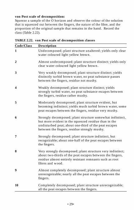
•29•
von Post scale of decomposition:Squeeze a sample of the O horizon and observe the colour of the solutionthat is squeezed out between the fingers, the nature of the fibre, and theproportion of the original sample that remains in the hand. Record theclass (Table 2.22).
TABLE 2.22. von Post scale of decomposition classes
Code/Class Description
1 Undecomposed; plant structure unaltered; yields only clearwater coloured light yellow brown.
2 Almost undecomposed; plant structure distinct; yields onlyclear water coloured light yellow brown.
3 Very weakly decomposed; plant structure distinct; yieldsdistinctly turbid brown water, no peat substance passesbetween the fingers, residue not mushy.
4 Weakly decomposed; plant structure distinct; yieldsstrongly turbid water, no peat substance escapes betweenthe fingers, residue rather mushy.
5 Moderately decomposed; plant structure evident, butbecoming indistinct; yields much turbid brown water, somepeat escapes between the fingers, residue very mushy.
6 Strongly decomposed; plant structure somewhat indistinct,but more evident in the squeezed residue than in theundisturbed peat; about one-third of the peat escapesbetween the fingers, residue strongly mushy.
7 Strongly decomposed; plant structure indistinct, butrecognizable; about one-half of the peat escapes betweenthe fingers.
8 Very strongly decomposed; plant structure very indistinct;about two-thirds of the peat escapes between the fingers,residue almost entirely resistant remnants such as rootfibres and wood.
9 Almost completely decomposed; plant structure almostunrecognizable; nearly all the peat escapes between thefingers.
10 Completely decomposed; plant structure unrecognizable;all the peat escapes between the fingers.
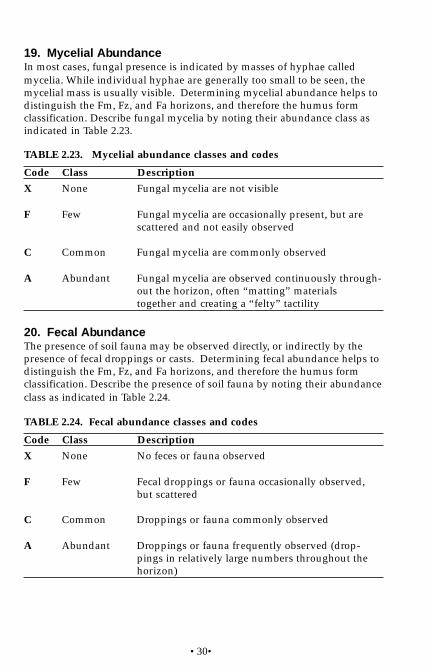
•30•
19. Mycelial AbundanceIn most cases, fungal presence is indicated by masses of hyphae calledmycelia. While individual hyphae are generally too small to be seen, themycelial mass is usually visible. Determining mycelial abundance helps todistinguish the Fm, Fz, and Fa horizons, and therefore the humus formclassification. Describe fungal mycelia by noting their abundance class asindicated in Table 2.23.
20. Fecal AbundanceThe presence of soil fauna may be observed directly, or indirectly by thepresence of fecal droppings or casts. Determining fecal abundance helps todistinguish the Fm, Fz, and Fa horizons, and therefore the humus formclassification. Describe the presence of soil fauna by noting their abundanceclass as indicated in Table 2.24.
TABLE 2.24. Fecal abundance classes and codes
Code Class Description
X None Fungal mycelia are not visible
F Few Fungal mycelia are occasionally present, but arescattered and not easily observed
C Common Fungal mycelia are commonly observed
A Abundant Fungal mycelia are observed continuously through-out the horizon, often “matting” materialstogether and creating a “felty” tactility
TABLE 2.23. Mycelial abundance classes and codes
Code Class Description
X None No feces or fauna observed
F Few Fecal droppings or fauna occasionally observed,but scattered
C Common Droppings or fauna commonly observed
A Abundant Droppings or fauna frequently observed (drop-pings in relatively large numbers throughout thehorizon)
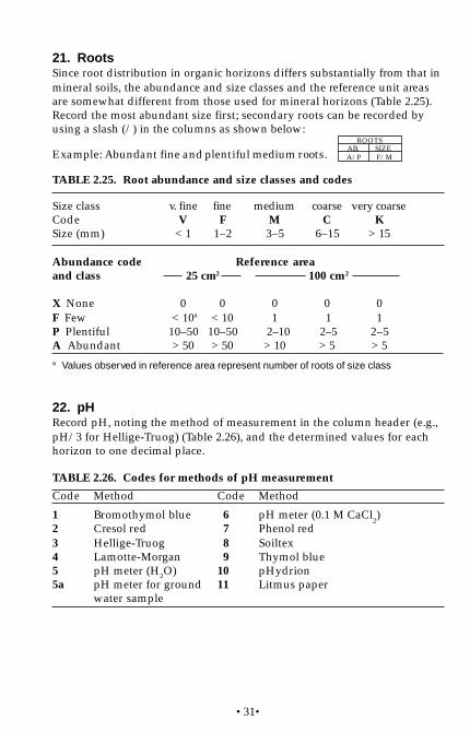
•31•
Size class v. fine fine medium coarse very coarseCode V F M C KSize (mm) < 1 1–2 3–5 6–15 > 15
Abundance code Reference areaand class 25 cm2 100 cm2
X None 0 0 0 0 0F Few < 10a < 10 1 1 1P Plentiful 10–50 10–50 2–10 2–5 2–5A Abundant > 50 > 50 > 10 > 5 > 5
21. RootsSince root distribution in organic horizons differs substantially from that inmineral soils, the abundance and size classes and the reference unit areasare somewhat different from those used for mineral horizons (Table 2.25).Record the most abundant size first; secondary roots can be recorded byusing a slash (/) in the columns as shown below:
Example: Abundant fine and plentiful medium roots.
22. pHRecord pH, noting the method of measurement in the column header (e.g.,pH/3 for Hellige-Truog) (Table 2.26), and the determined values for eachhorizon to one decimal place.
TABLE 2.25. Root abundance and size classes and codes
ROOTSAB.A/P
SIZEF/M
Code Method Code Method
1 Bromothymol blue 6 pH meter (0.1 M CaCl2)
2 Cresol red 7 Phenol red3 Hellige-Truog 8 Soiltex4 Lamotte-Morgan 9 Thymol blue5 pH meter (H2O) 10 pHydrion5a pH meter for ground 11 Litmus paper
water sample
TABLE 2.26. Codes for methods of pH measurement
a Values observed in reference area represent number of roots of size class

•32•
Character:This describes tactile qualities, particulate shapes, and other noteworthyqualities of materials in organic horizons. Determining the characterrequires a qualitative examination of the fabric. Use the codes in Table 2.28to describe character.
23. Comments SectionRecord any observations or measurements that are unique, unconforming,or could be of particular significance to the study, classification, or manage-ment interpretations. Examples include: consistence, character, faunalspecies, colour of mycelium, percentage of decaying wood, presence ofcharcoal, and disturbance history. When coding a property, be sure to notethe property being described.
Consistence:This describes the nature and strength of forces holding materials together.It is determined by the kind of deformation or rupture that occurs whenpressure is applied and then released. Use the codes in Table 2.27 todescribe consistency.
TABLE 2.27. Consistency classes and codes
Code Class Description
LO Loose Material has no consistence
FR Friable Material crumbles easily under gentle pressure
FM Firm Material can be crushed under moderate pressure;resistance is noticeable
PL Pliable Material is soft and plastic
RE Resilient Material is springy or elastic; assumes its original shapeafter pressure is released
TE Tenacious Material is cohesive and not easily pulled apart
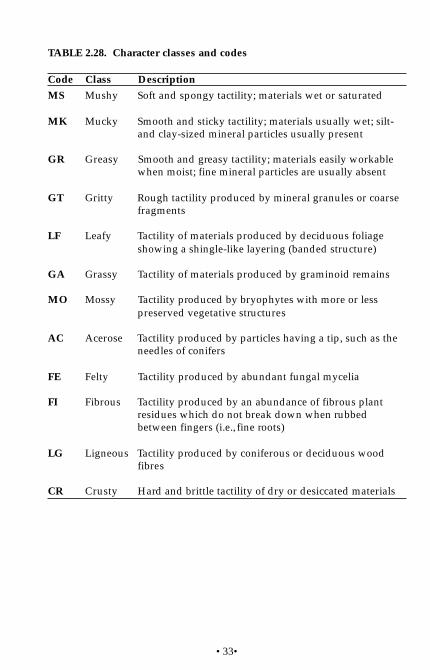
•33•
TABLE 2.28. Character classes and codes
Code Class Description
MS Mushy Soft and spongy tactility; materials wet or saturated
MK Mucky Smooth and sticky tactility; materials usually wet; silt-and clay-sized mineral particles usually present
GR Greasy Smooth and greasy tactility; materials easily workablewhen moist; fine mineral particles are usually absent
GT Gritty Rough tactility produced by mineral granules or coarsefragments
LF Leafy Tactility of materials produced by deciduous foliageshowing a shingle-like layering (banded structure)
GA Grassy Tactility of materials produced by graminoid remains
MO Mossy Tactility produced by bryophytes with more or lesspreserved vegetative structures
AC Acerose Tactility produced by particles having a tip, such as theneedles of conifers
FE Felty Tactility produced by abundant fungal mycelia
FI Fibrous Tactility produced by an abundance of fibrous plantresidues which do not break down when rubbedbetween fingers (i.e., fine roots)
LG Ligneous Tactility produced by coniferous or deciduous woodfibres
CR Crusty Hard and brittle tactility of dry or desiccated materials

•34•
Fauna:When describing soil fauna, use the name (Figure 2.3), e.g., few earth-worms, several nematodes.
FIGURE 2.3. Major kinds of soil fauna.
Label Fauna Label Fauna
A Mites (Acarina) G Woodlice (Isopoda)B Springtails H Centipedes and millipedes
(Collembola) (Myriapoda)C Spiders (Araneida) I Termites (Isoptera)D Fly larvae (Diptera) J Earthworms (Lumbricida)E Beetles and larvae K Potworms (Enchytraeida)
(Coleoptera)F Ants (Hymenoptera) L Nematodes (Nematoda)

•35•
Mineral Horizons/Layers
The soil horizon and layer definitions and methods for field descriptionthat follow are taken or modified from Agriculture Canada Expert Commit-tee on Soil Survey (1997), Green et al. (1993), and Luttmerding et al. (1990).
24. Horizon/LayerRecord the mineral horizon or layer designation followed by lowercasemodifiers, e.g., Btg.
Codes for major horizons:A Mineral horizon, containing < 17% organic C by mass, that has formed
at or near the soil surface in the zone of leaching or eluviation oforganic materials in solution or suspension, or of maximum in situaccumulation of organic matter, or both.
B Mineral horizon characterized by enrichment in organic matter,sequioxides, or clay; or by the development of soil structure; or by achange of colour denoting hydrolysis, reduction, or oxidation.
C Mineral horizon comparatively unaffected by the pedogenic processesoperative in the A and B horizons, except the process of gleying (Cg),and the accumulation of calcium and magnesium carbonates (Cca)and more soluble salts (Cs, Csa).
Codes for layers:R Consolidated bedrock layer which is too hard to break with the hands.
W Layer of water in Gleysolic, Organic, or Cryosolic soils.
Lowercase modifiers:b Buried soil horizon.
c Irreversibly cemented horizon (ortstein, placic, duric, and CaCO3
cemented layers are examples).
ca Horizon > 10 cm thick of secondary carbonate enrichment in whichthe concentration of lime exceeds that in the unenriched parentmaterial.
cc Irreversibly cemented concretions.
e Horizon characterized by the eluviation of clay, Fe, Al, or organicmatter alone or in combination.

•36•
f Horizon enriched with amorphous material, principally Al and Fecombined with organic matter. It must have a hue of 7.5YR or redder,or its hue must be 10YR near the upper boundary and becomesyellower with depth. When moist the chroma is higher than three orthe value is three or less. It is used primarily with the Bf, Bhf, Bfg, andBgf codes. The following f horizons are differentiated on the basis ofthe organic C content:
Bf 0.5–5% organic CBhf > 5% organic C
g Horizon characterized by gray colours, or prominent mottling, orboth, which indicates of permanent or periodic intense reduction.Chromas of the matrix are generally one or less. It is used with theAeg, Bg, Bfg, Bgf, Bhfg, Btg, Cg, Ckg codes, and others. When usedwith the Ae, Bf, Bhf, and Bt codes, the limits set for the other modifiersmust be met. The Bgf horizons are usually prominently mottled; morethan half of the soil material occurs as mottles of high chroma. TheBgf horizons occur in Fera Gleysols and Fera Humic Gleysols andpossibly below the Bfg of gleyed Podzols.
h Horizon enriched with organic matter. It is used with the Ah, Ahe, Bh,and Bhf codes.
Ah - An A horizon enriched with humified organic matter; at least onecolour value unit lower that the underlying horizon, or 0.5% more or-ganic C than the C horizon or both.
Ahe - An Ah horizon that has undergone eluviation as evidenced bystreaks and splotches of different shades of gray, and often by platedstructure.
Bh - Contains > 1% organic C with less than 0.3% pyrophosphate-ex-tractable Fe [Fe(p)] and a ratio of C : Fe(p) of 20 or more (very rare inBritish Columbia).
Bhf - Defined under f above.
j Used with e, f, g, n, and t to denote an expression of, but failure tomeet, the specified limits of the letter code it modifies. It is placed tothe right of the letter it modifies.
k Denotes the presence of carbonate as indicated by visible effervescencewhen a dilute HCl solution is added.

•37•
m Horizon slightly altered by hydrolysis, oxidation, or solution, or allthree to give a change in colour or structure, or both. It is used withthe Bm, Bmgj, Bmk, and Bms codes.
It has:1. Evidence of one of or more of the following:
• higher chromas and redder hues than the underlyinghorizons;
• enrichment or complete removal of carbonates either asBmk or Bm; and/or
• change in structure from that of the original material.2. Illuviation too slight to meet requirements of a Bt or podzolic B.3. No cementation or induration and lacks a brittle consistence
when moist.
n Horizon with distinctive prismatic or columnar structure, darkcoatings on ped surfaces, and hard to very hard consistence when dry;the exchangeable Ca to exchangeable Na is 10 or less. It is used withBn or Bnt codes.
p Horizon disturbed by human activities, such as cultivation, logging,and habitation.
s Horizon with salts, including gypsum, which may be detected ascrystal or veins, or as surface crusts of salt crystals. It is used with anycombination of horizon codes.
sa Horizon > 10 cm thick with secondary enrichment of salts moresoluble than Ca and Mg carbonates; the concentration of salts exceedsthat in the unenriched parent material.
t An illuvial horizon enriched with silicate clay. It is used with the Bt,Btg, and Bnt codes and may be modified by j.To use Bt:• The horizon must be at least 5 cm thick.• If any part of an the eluvial horizon has < 15% total clay in the
fine fraction (< 2 mm), the Bt horizon must contain at least 3% moreclay and if > 40% total clay, then it must contain at least 8% more clay.If the eluvial horizon has > 15% and < 40% clay in the fine fraction,then the ratio of the clay in the Bt to that of the eluvial horizon mustbe 1.2 or more (e.g., Ae 25 % clay; Bt at least 30% clay).
• In massive soils, there should be oriented clay in pores and as bridgesbetween sand grains.
• If peds are present, clay films (skins) should be visible on ped surfacesand in pores.

•38•
u Horizon that is markedly disrupted by physical (e.g., blowdown oftrees, mass movement, etc.) or faunal processes (e.g., burrowinganimals), but not from cryoturbation.
x Horizon of fragipan character; loamy subsurface horizon of high bulkdensity and very low organic matter. When dry, it is hard and seemsto be cemented; when moist is has moderate to weak brittleness. Air-dried clods slake (crumble) in water.
y Horizon affected by cryoturbation. It is used with any combination ofhorizon codes.
z A frozen layer, it may be used with any horizon or layer code.
Mineral diagnostic horizons:Chernozemic A• At least 10 cm thick;• Colour value darker than 5.5 dry and 3.5 moist, chroma is lower
than 3.5 moist;• Organic C content 1–17% and C:N ratio < 17;• Structure, when dry, is neither massive and hard, nor single
grained; and• Mean annual soil temperature of 0o C or higher and a soil moisture
regime subclass drier than humid.
Duric horizonA strongly cemented horizon that does not satisfy the criteria of a podzolicB horizon. Usually has an abrupt upper boundary and a diffuse lowerboundary. Air-dried clods do not hydrate in water, and moist clods at least3 cm thick usually can not be broken in the hands.
Fragipan horizonSee definition of “x” above.
Ortstein horizonA strongly cemented Bh, Bhf, of Bf horizon at least 3 cm thick which occursin more than one-third of the exposed pedon. Generally reddish brown tovery dark reddish brown.
Placic horizonA thin layer (commonly 5 mm or less thick) or a series of thin layers that areirregular or involuted, hard, impervious, often vitreous, and dark reddishbrown to black.
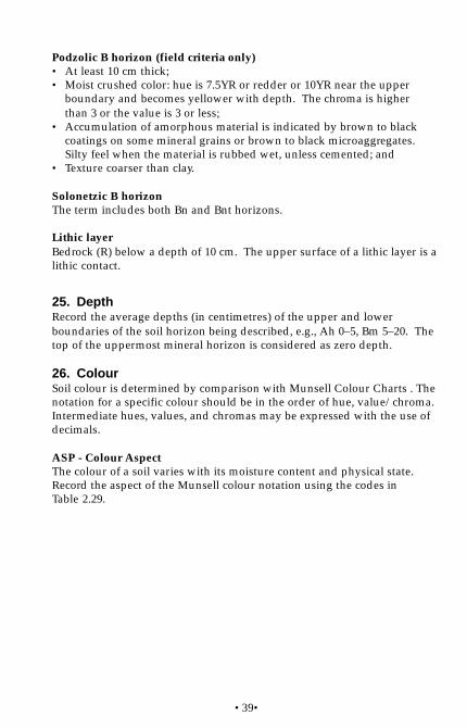
•39•
Podzolic B horizon (field criteria only)• At least 10 cm thick;• Moist crushed color: hue is 7.5YR or redder or 10YR near the upper
boundary and becomes yellower with depth. The chroma is higherthan 3 or the value is 3 or less;
• Accumulation of amorphous material is indicated by brown to blackcoatings on some mineral grains or brown to black microaggregates.Silty feel when the material is rubbed wet, unless cemented; and
• Texture coarser than clay.
Solonetzic B horizonThe term includes both Bn and Bnt horizons.
Lithic layerBedrock (R) below a depth of 10 cm. The upper surface of a lithic layer is alithic contact.
25. DepthRecord the average depths (in centimetres) of the upper and lowerboundaries of the soil horizon being described, e.g., Ah 0–5, Bm 5–20. Thetop of the uppermost mineral horizon is considered as zero depth.
26. ColourSoil colour is determined by comparison with Munsell Colour Charts . Thenotation for a specific colour should be in the order of hue, value/chroma.Intermediate hues, values, and chromas may be expressed with the use ofdecimals.
ASP - Colour AspectThe colour of a soil varies with its moisture content and physical state.Record the aspect of the Munsell colour notation using the codes inTable 2.29.
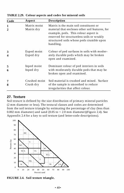
•40•
TABLE 2.29. Colour aspects and codes for mineral soils
Per
cent
cla
y
Percent sand
100
90
80
70
60
50
40
30
20
10
00 10 20 30 40 50 60 70 80 90 100
HC
C
SiC
SiCL CL
SCL
LSiL
Si SL LS S
SC
27. TextureSoil texture is defined by the size distribution of primary mineral particles(2 mm diameter or less). The textural classes and codes are determinedfrom the soil texture triangle by estimating the percentage of clay (less than0.002 mm diameter) and sand (0.05 to < 2.0 mm diameter)(Figure 2.4). SeeAppendix 2.4 for a key to soil texture (and letter-code descriptions).
FIGURE 2.4. Soil texture triangle.
Description
Matrix is the main soil constituent ormaterial that encloses other soil features, forexample, peds. This colour aspect isreserved for structureless soils or weaklystructured soils whose peds crumble uponhandling.
Colour of ped surfaces in soils with moder-ately durable peds which may be brokenopen and examined.
Dominant colour of ped interiors in soilswith moderately durable peds that may bebroken open and examined.
Soil material is crushed and mixed. Surfaceof the sample is smoothed to reduceirregularities that affect colour.
Aspect
Matrix moistMatrix dry
Exped moistExped dry
Inped moistInped dry
Crushed moistCrush dry
Code
12
34
56
78

•41•
Size class Very fine Fine Medium CoarseCode V F M CSize (mm) < 1 1 to 2 3 to 5 > 5
Abundance codeand classX None 0 0 0 0F Few < 10a < 10 1 1P Plentiful 10–100 10–100 2–10 2–5A Abundant > 100 > 100 > 10 > 5
28. Percent Coarse FragmentsEstimate the percent coarse fragment (> 2 mm diameter) volume in eachsize class and record the total percent. Describe the coarse fragment shapeusing the type codes in Table 2.30.
a type codes: R = rounded; S = subrounded and subangular; A = angular; T = thin, flat.
29. RootsDescribe roots by noting their abundance and size (Table 2.31). Record themost abundant size first; secondary roots can be recorded by using a slash(/) in the columns (see example in Item 21).
Shape type: Shape type:R, S, Aa T
Size Classes Diameter (cm) Length (cm)
G - Gravel < 7.5 < 15C - Cobbles 7.5–25 15–38S - Stones and >25 > 38
boulders
TABLE 2.30. Size classes and type codes for coarse fragments
TABLE 2.31. Root abundance and size classes and codes
a Values represent number of roots of size class observed in reference area of 100 cm2.
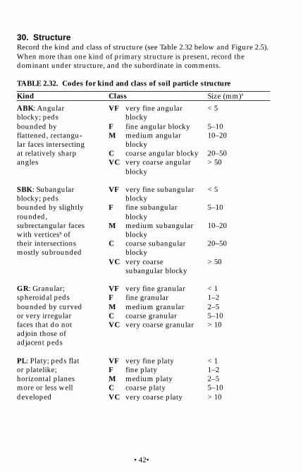
•42•
30. StructureRecord the kind and class of structure (see Table 2.32 below and Figure 2.5).When more than one kind of primary structure is present, record thedominant under structure, and the subordinate in comments.
Kind
ABK: Angularblocky; pedsbounded byflattened, rectangu-lar faces intersectingat relatively sharpangles
SBK: Subangularblocky; pedsbounded by slightlyrounded,subrectangular faceswith verticesb oftheir intersectionsmostly subrounded
GR: Granular;spheroidal pedsbounded by curvedor very irregularfaces that do notadjoin those ofadjacent peds
PL: Platy; peds flator platelike;horizontal planesmore or less welldeveloped
Class
VF very fine angularblocky
F fine angular blockyM medium angular
blockyC coarse angular blockyVC very coarse angular
blocky
VF very fine subangularblocky
F fine subangularblocky
M medium subangularblocky
C coarse subangularblocky
VC very coarsesubangular blocky
VF very fine granularF fine granularM medium granularC coarse granularVC very coarse granular
VF very fine platyF fine platyM medium platyC coarse platyVC very coarse platy
Size (mm)a
< 5
5–1010–20
20–50> 50
< 5
5–10
10–20
20–50
> 50
< 11–22–55–10> 10
< 11–22–55–10> 10
TABLE 2.32. Codes for kind and class of soil particle structure

•43•
Kind
PR: Prismatic;vertical faces of pedswell defined andverticesb angular(edges sharp); prismtops essentially flat
COL: Columnar;vertical edges neartop of columns notsharp (verticesb
subrounded);column tops flat,rounded, orirregular
SGR: single grained
MA: Massive
CDY:
Class
VF very fine prismaticF fine prismaticM medium prismaticC coarse prismaticVC very coarse pris-
matic
VF very fine columnarF fine columnarM medium columnarC coarse columnarVC very coarse colum-
nar
Loose, incoherent mass ofindividual primaryparticles, as in sands
Amorphous; a coherentmass showing noevidence of any distinctarrangement of soilparticles; separates intoclusters of particles, notpeds
Cloddy; not a structure,used to indicate thecondition of someploughed surfaces.
Size (mm)a
< 1010–2020–5050–100> 100
< 1010–2020–5050–100> 100
a The size limits refer to measurements in the smallest dimension of platy, prismatic,and columnar peds, and to the largest of the nearly equal dimensions of blocky andgranular peds.
b Definition of vertex (plural, vertices): the intersection of two planes of a geometricalfigure.

•44•
TABLE 2.34. Contrast codes for mottles
TABLE 2.33. Abundance and size codes for mottles
Grade The degree of distinctness of aggregation of soil particles. If gradeof structure is described, record with class code separated by a slash (e.g.,S/VC = strong/very coarse).
W = WeakWM = Weak to moderateM = ModerateMS = Moderate to strongS = Strong
31. pHRecord pH by noting the method of measurement (see Table 2.26 underItem 22) and the determined values to one decimal place.
32. CommentsRecord any observations or measurements that are unique, unconforming,or could be of particular significance to the study, classification, or manage-ment interpretations. Examples include: colour and description of mottles(see colour section), description of clay films, and porosity.
Mottling:Described by recording abundance, size, and contrast and colour (see Tables2.33 and 2.34). Use Munsell Colour Charts, defaulting to aspect 7, crushedmoist, unless otherwise noted. For example, FMD 7.5YR mottles = few,medium, distinct, strong brown (crushed moist) mottles.
Abundance Size
Code Class % of Code Class Diameterexposed (mm)surface
F Few < 2 F Fine < 5C Common 2–20 M Medium 5–15M Many > 20 C Coarse > 15
Code Description
F Faint: Evident only on close examination. Faint mottles commonlyhave the same hue as the colour to which they are compared anddiffer by no more than 1 unit of chroma or 2 units of value. Somefaint mottles of similar but low chroma and value can differ by 2.5units of hue.
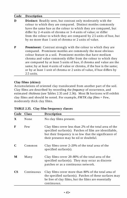
•45•
Clay films (skins):Accumulations of oriented clay translocated from another part of the soil.Clay films are described by recording the frequency of occurrence, andestimated thickness (see Tables 2.35 and 2.36). Most Bt horizons will exhibitclay films and should be noted. For example, FMTK clay films = Few,moderately thick clay films.
Code Description
D Distinct: Readily seen, but contrast only moderately with thecolour to which they are compared. Distinct mottles commonlyhave the same hue as the colour to which they are compared, butdiffer by 2–4 units of chroma or 3–4 units of value; or differfrom the colour to which they are compared by 2.5 units of hue, butby no more than 1 unit of chroma or 2 units of value.
P Prominent: Contrast strongly with the colour to which they arecompared. Prominent mottles are commonly the most obviouscolour feature in a soil. Prominent mottles that have mediumchroma and value commonly differ from the colour to which theyare compared by at least 5 units of hue, if chroma and value are thesame; by at least 4 units of value or chroma, if the hue is the same;or by at least 1 unit of chroma or 2 units of value, if hue differs by2.5 units.
TABLE 2.35. Clay film frequency classes
Description
No clay films present.
Clay films cover less than 2% of the total area of thespecified surface(s). Patches of film are identifiable,but their frequency is so low that the significance oftheir presence may be nil or doubtful.
Clay films cover 2–20% of the total area of thespecified surface(s).
Clay films cover 20–80% of the total area of thespecified surface(s). They may occur as discretepatches or as a continuous network.
Clay films cover more than 80% of the total area ofthe specified surface(s). Patches of these surfaces maybe free of clay films, but the films are essentiallycontinuous.
Code
X
F
C
M
CS
Class
None
Few
Common
Many
Continuous
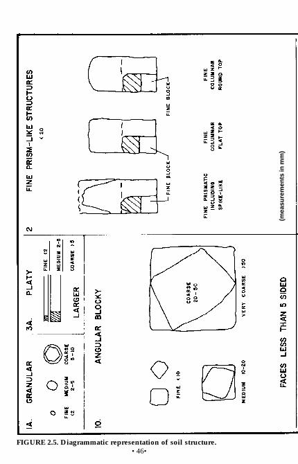
•46•FIGURE 2.5. Diagrammatic representation of soil structure.
(mea
sure
men
ts in
mm
)

•47•FIGURE 2.5. (continued).
SC
ALE
IN M
M.
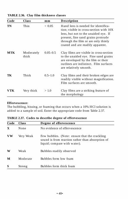
•48•
TABLE 2.36. Clay film thickness classes
Effervescence:The bubbling, hissing, or foaming that occurs when a 10% HCl solution isadded to a sample of soil. Enter the appropriate code from Table 2.37.
TABLE 2.37. Codes to describe degree of effervescence
Description
Hand lens is needed for identifica-tion; visible in cross-section with 10Xlens, but not to the unaided eye. Ifpresent, fine sand grains protrudethrough the film or are only thinlycoated and are readily apparent.
Clay films are visible in cross-sectionto the unaided eye. Fine sand grainsare enveloped by the film or theiroutlines are indistinct. Film surfacesare relatively smooth.
Clay films and their broken edges arereadily visible without magnification.Film surfaces are smooth.
Clay films are a striking feature ofthe morphology
mm
< 0.05
0.05–0.5
0.5–1.0
> 1.0
Class
Thin
Moderatelythick
Thick
Very thick
Code
TN
MTK
TK
VTK
Degree of effervescence
No evidence of effervescence
Few bubbles. (Note: ensure that the cracklingsound is from reaction rather than absorption ofliquid; compare with water).
Bubbles readily observed
Bubbles form low foam
Bubbles form thick foam
Code Class
X None
VW Very Weak
W Weak
M Moderate
S Strong

•49•
Horizon porosity:An estimate of total pore volume that reflects the combined effects of soilstructure and density. Record porosity classes for mineral horizons asdescribed in Table 2.38.
34. NotesUse this section to summarize or describe soil features not otherwiserecorded on the form or that are significant to the study, classifications, ormanagement interpretations.
33. Profile diagramSketch a cross-sectional profile diagram of the horizon boundaries, andadd other significant features (relative coarse fragment distribution andsize, piping, turbation, seepage, water table, lithic contact, etc.) (seeexample, Figure 2.6.
AeFm
Bf1
Bf2
BC
C
PROFILEDIAGRAM
20
40
60
0
10
TABLE 2.38. Mineral horizon porosity classes
FIGURE 2.6. Example of profile diagram.
Description
Closely packed structureless soil material; highlycompacted material.
Horizons with weak to moderate structure andmoderately close packing; closely packed soilswith large, well-developed peds.
Horizons that are loosely packed, and/or verywell structured with small peds.
Code Porosity class
S Slightly porous
M Moderatelyporous
H Highly porous

•50•

•51•
Appendix 2.1 Codes for Soil Orders,Great Groups and Subgroups
Brunisolic OrderMelanic Brunisol MBOrthic O.MBEluviated E.MBGleyed GL.MBGleyed Eluviated GLE.MB
Eutric Brunisol EBOrthic O.EBEluviated E.EBGleyed GL.EBGleyed Eluviated GLE.EB
Sombric Brunisol SBOrthic O.SBEluviated E.SBDuric DU.SBGleyed GL.SBGleyed Eluviated GLE.SB
Dystric Brunisol DYBOrthic O.DYBEluviated E.DYBDuric DU.DYBGleyed GL.DYBGleyed Eluviated GLE.DYB
Chernozemic OrderBrown Chernozem BCOrthic O.BCRego R.BCCalcareous CA.BCEluviated E.BCSolonetzic SZ.BCVertic V.BCGleyed GL.BCGleyed Rego GLR.BCGleyed Calcareous GLA.BCGleyed Eluviated GLE.BCGleyed Solonetzic GLSZ.BCGleyed Vertic GLV.BC
Dark Brown Chernozem DBCOrthic O.DBCRego R.DBCCalcareous CA.DBCEluviated E.DBCSolonetzic SZ.DBCGleyed GL.DBCGleyed Rego GLR.DBCGleyed Calcareous GLCA.DBCGleyed Eluviated GLE.DBCGleyed Solonetzic GLSZ.DBC
Black Chernozem BLCOrthic O.BLCRego R.BLCCalcareous CA.BLCEluviated E.BLCSolonetzic SZ.BLCVertic V.BLCGleyed GL.BLCGleyed Rego GLR.BLCGleyed Calcareous GLCA.BLCGleyed Eluviated GLE.BLCGleyed Solonetzic GLSZ.BLCGleyed Vertic GLV.BLC
Dark Gray Chernozem DGCOrthic O.DGCRego R.DGCCalcareous CA.DGCSolonetzic SZ.DGCVertic V.DGCGleyed GL.DGCGleyed Rego GLR.DGCGleyed Calcareous GLCA.DGCGleyed Solonetzic GLSZ.DGCGleyed Vertic GLV.DGC

•52•
Cryosolic OrderTurbic Cryosol TCOrthic Eutric OE.TCOrthic Dystric OD.TCBrunisolic Eutric BRE.TCBrunisolic Dystric BRD.TCHistic Eutric HE.TCHistic Dystric HD.TCLuvisolic L.TCRegosolic R.TCGleysolic GL.TC
Static Cryosol SCOrthic Eutric OE.SCOrthic Dystric OD.SCBrunisolic Eutric BRE.SCBrunisolic Dystric BRD.SCHistic Eutric HE.SCHistic Dystric HD.SCLuvisolic L.SCGleysolic Static Cryosol GL.SCRegosolic Static Cryosol R.SC
Organic Cryosol OCFibric FI.OCMesic ME.OCHumic HU.OCTerric Fibric TFI.OCTerric Mesic TME.OCTerric Humic THU.OCGlacic GC.OC
Gleysolic OrderLuvic Gleysol LGSolonetzic SZ.LGFragic FR.LGHumic HU.LGFera FE.LGOrthic O.LGVertic V.LG
Humic Gleysol HGSolonetzic SZ.HGFera FE.HGOrthic O.HG
Rego R.HGVertic V.HG
Gleysol GSolonetzic SZ.GFera FE.GOrthic O.GRego R.GVertic V.G
Luvisolic OrderGray Brown Luvisol GBLOrthic O.GBLBrunisolic BR.GBLPodzolic PZ.GBLVertic V.GBLGleyed GL.GBLGleyed Brunisolic GLBR.GBLGleyed Podzolic GLPZ.GBLGleyed Vertic GLV.GBL
Gray Luvisol GLOrthic O.GLDark D.GLBrunisolic BR.GLPodzolic PZ.GLSolonetzic SZ.GLFragic FR.GLVertic V.GLGleyed GL.GLGleyed Dark GLD.GLGleyed Brunisolic GLBR.GLGleyed Podzolic GLPZ.GLGleyed Solonetzic GLSZ.GLGleyed Fragic GLFR.GLGleyed Vertic GLV.GL
Organic OrderFibrisol FTypic TY.FMesic ME.FHumic HU.FLimnic LM.FCumulic CU.FTerric T.F
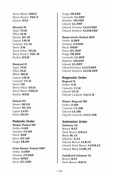
•53•
Terric Mesic TME.FTerric Humic THU.FHydric HY.F
Mesisol MTypic TY.MFibric FI.MHumic HU.MLimnic LM.MCumulic CU.MTerric T.M.Terric Fibric TFI.MTerric Humic THU.MHydric HY.M
Humisol HTypic TY.HFibric FI.HMesic ME.HLimnic LM.HCumulic CU.HTerric T.HTerric Fibric TFI.HTerric Mesic TME.HHydric HY.H
Folisol FOHemic HE.FOHumic HU.FOLignic LI.FOHistic HI.FO
Podzolic OrderHumic Podzol HPOrthic O.HPOrtstein OT.HPPlacic P.HPDuric DU.HPFragic FR.HP
Ferro-Humic Podzol FHPOrthic O.FHPOrtstein OT.FHPPlacic P.FHPDuric DU.FHP
Fragic FR.FHPLuvisolic LU.FHPSombric SM.FHPGleyed GL.FHPGleyed Ortstein GLOT.FHPGleyed Sombric GLSM.FHP
Humo-Ferric Podzol HFPOrthic O.HFPOrtstein OT.HFPPlacic P.HFPDuric DU.HFPFragic FR.HFPLuvisolic LU.HFPSombric SM.HFPGleyed GL.HFPGleyedOrtstein GLOT.HFPGleyed Sombric GLSM.HFP
Regosolic OrderRegosol ROrthic O.RCumulic CU.RGleyed GL.RGleyed Cumulic GLCU.R
Humic Regosol HROrthic O.HRCumulic CU.HRGleyed GL.HRGleyed Cumulic GLCU.HR
Solonetzic OrderSolonetz SZBrown B.SZDark Brown DB.SZBlack BL.SZAlkaline A.SZGleyed Brown GLB.SZGleyed Dark Brown GLDB.SZGleyed Black GLBL.SZ
Solodized Solonetz SSBrown B.SSDark Brown DB.SS
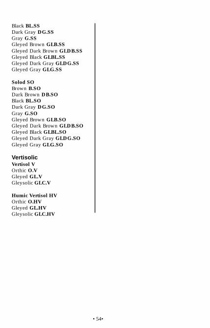
•54•
Black BL.SSDark Gray DG.SSGray G.SSGleyed Brown GLB.SSGleyed Dark Brown GLDB.SSGleyed Black GLBL.SSGleyed Dark Gray GLDG.SSGleyed Gray GLG.SS
Solod SOBrown B.SODark Brown DB.SOBlack BL.SODark Gray DG.SOGray G.SOGleyed Brown GLB.SOGleyed Dark Brown GLDB.SOGleyed Black GLBL.SOGleyed Dark Gray GLDG.SOGleyed Gray GLG.SO
VertisolicVertisol VOrthic O.VGleyed GL.VGleysolic GLC.V
Humic Vertisol HVOrthic O.HVGleyed GL.HVGleysolic GLC.HV
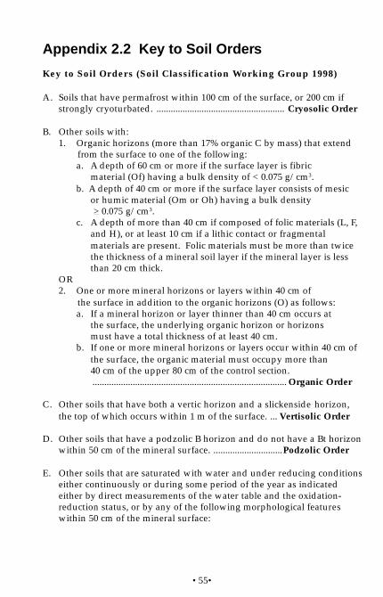
•55•
Key to Soil Orders (Soil Classification Working Group 1998)
A. Soils that have permafrost within 100 cm of the surface, or 200 cm ifstrongly cryoturbated. ...................................................... Cryosolic Order
B. Other soils with:1. Organic horizons (more than 17% organic C by mass) that extend
from the surface to one of the following:a. A depth of 60 cm or more if the surface layer is fibric
material (Of) having a bulk density of < 0.075 g/cm3.b. A depth of 40 cm or more if the surface layer consists of mesic
or humic material (Om or Oh) having a bulk density > 0.075 g/cm3.
c. A depth of more than 40 cm if composed of folic materials (L, F,and H), or at least 10 cm if a lithic contact or fragmentalmaterials are present. Folic materials must be more than twicethe thickness of a mineral soil layer if the mineral layer is lessthan 20 cm thick.
OR2. One or more mineral horizons or layers within 40 cm of
the surface in addition to the organic horizons (O) as follows:a. If a mineral horizon or layer thinner than 40 cm occurs at
the surface, the underlying organic horizon or horizonsmust have a total thickness of at least 40 cm.
b. If one or more mineral horizons or layers occur within 40 cm ofthe surface, the organic material must occupy more than40 cm of the upper 80 cm of the control section................................................................................... Organic Order
C. Other soils that have both a vertic horizon and a slickenside horizon,the top of which occurs within 1 m of the surface. ... Vertisolic Order
D. Other soils that have a podzolic B horizon and do not have a Bt horizonwithin 50 cm of the mineral surface. .............................Podzolic Order
E. Other soils that are saturated with water and under reducing conditionseither continuously or during some period of the year as indicatedeither by direct measurements of the water table and the oxidation-reduction status, or by any of the following morphological featureswithin 50 cm of the mineral surface:
Appendix 2.2 Key to Soil Orders

•56•
1. For all but red soil materials (hue 5YR or redder and colour fadesslowly on dithionite treatment).
a. Chromas of 1 or less, without mottles, on ped surfaces or inthe matrix if peds are lacking in materials that develophigher chromas under oxidizing conditions.
b. Chromas of 2 or less, in hues of 10YR and 7.5YR, on pedsurfaces or in the matrix if peds are lacking, accompanied byprominent mottles.
c. Chromas of 3 or less, in hues yellower than 10YR, on pedsurfaces or in the matrix if peds are lacking, accompanied byprominent mottles.
d. Hues bluer than 10Y, with or without mottles, on ped surfacesor in the matrix if peds are lacking. ................ Gleysolic Order
2. Other soils that have a solonetzic B horizon. ..... Solonetzic Order
G. Other soils that have a chernozemic A horizon and any one of thefollowing:1. No Ae horizon.2. A weakly expressed Ae horizon (Aej) with a dry colour value
lower than 5.3. An Ae horizon thinner than an overlying Ah or Ap horizon that
does not appear to be eluviated.4. An Ae horizon not more than 5 cm thick if the chernozemic A is
eluviated (Ahe), as indicated by grey streaks and splotches whenthe soil is dry. ................................................... Chernozemic Order
H. Other soils that have a Bt horizon. ............................. Luvisolic Order
I. Other soils that have either Bm, Btj, or Bfj horizons at least 5 cm thick,or a Bf horizon less than 10 cm in thickness. .......... Brunisolic Order
J. Other soils. ...................................................................... Regosolic Order
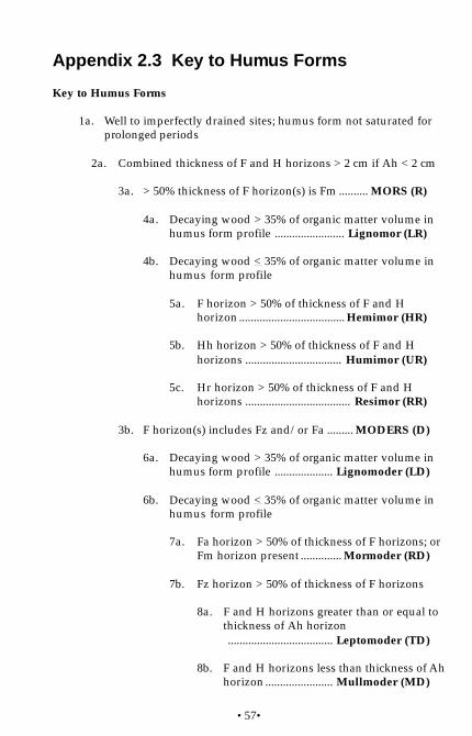
•57•
Key to Humus Forms
1a. Well to imperfectly drained sites; humus form not saturated forprolonged periods
2a. Combined thickness of F and H horizons > 2 cm if Ah < 2 cm
3a. > 50% thickness of F horizon(s) is Fm .......... MORS (R)
4a. Decaying wood > 35% of organic matter volume inhumus form profile ........................ Lignomor (LR)
4b. Decaying wood < 35% of organic matter volume inhumus form profile
5a. F horizon > 50% of thickness of F and Hhorizon .................................... Hemimor (HR)
5b. Hh horizon > 50% of thickness of F and Hhorizons ................................. Humimor (UR)
5c. Hr horizon > 50% of thickness of F and Hhorizons .................................... Resimor (RR)
3b. F horizon(s) includes Fz and/or Fa ......... MODERS (D)
6a. Decaying wood > 35% of organic matter volume inhumus form profile .................... Lignomoder (LD)
6b. Decaying wood < 35% of organic matter volume inhumus form profile
7a. Fa horizon > 50% of thickness of F horizons; orFm horizon present .............. Mormoder (RD)
7b. Fz horizon > 50% of thickness of F horizons
8a. F and H horizons greater than or equal tothickness of Ah horizon.................................... Leptomoder (TD)
8b. F and H horizons less than thickness of Ahhorizon ....................... Mullmoder (MD)
Appendix 2.3 Key to Humus Forms

•58•
2b. Combined thickness of F and H horizons < 2 cm and Ahhorizon > 2cm ...................................................... MULLS (L)9a. Rhizogenous Ah horizon formed from decomposition
of dense fine roots ............................... Rhizomull (ZL)
9b. Zoogenous Ah horizon formed through actions ofabundant earthworms ....................... Vermimull (VL)
1b. Poor to very poorly drained sites; humus form saturated forprolonged periods
10a. Combined thickness of F, H, and O horizons < 2 cm and Ahhorizon > 2 cm ............................................ Hydromull (YL)
10b. Combined thickness of F, H, and O horizons > 2 cm ifAh < 2 cm
11a. Thickness of F and H horizons > O horizons
12a. F horizon(s) is Fm ...................... Hydromor (YR)
12b. F horizon(s) includes Fz and/or Fa................................................. Hydromoder (YD)
11b. Combined thickness of O horizons greater than F andH horizons
13a. Of horizon > 50% of thickness of O horizons......................................................... Fibrimor (FR)
13b. Om horizon > 50% of thickness of O horizons....................................................... Mesimor (MR)
13c. Oh horizon > 50% of thickness of O horizons................................................... Saprimoder (SD)
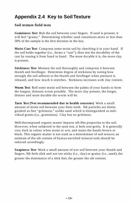
•59•
Soil texture field tests
Graininess Test Rub the soil between your fingers. If sand is present, itwill feel “grainy.” Determining whether sand constitutes more or less than50% of the sample is the first decision in the key.
Moist Cast Test Compress some moist soil by clenching it in your hand. Ifthe soil holds together (i.e., forms a “cast”), then test the durability of thecast by tossing it from hand to hand. The more durable it is, the more clayis present.
Stickiness Test Moisten the soil thoroughly and compress it betweenthumb and forefinger. Determine degree of stickiness by noting howstrongly the soil adheres to the thumb and forefinger when pressure isreleased, and how much it stretches. Stickiness increases with clay content.
Worm Test Roll some moist soil between the palms of your hands to formthe longest, thinnest worm possible. The more clay present, the longer,thinner and more durable the worm will be.
Taste Test (Not recommended due to health concerns) Work a smallamount of moist soil between your front teeth. Silt particles are distin-guished as fine “grittiness,” unlike sand which is distinguished as indi-vidual grains (i.e., graininess). Clay has no grittiness.
Well-decomposed organic matter imparts silt-like properties to the soil.However, when subjected to the taste test, it feels non-gritty. It is generallyvery dark in colour when moist or wet, and stains the hands brown orblack. This organic matter is not used as a determinant of soil texture; anestimate of the silt content of humus-enriched mineral soils should bereduced accordingly.
Soapiness Test Work a small amount of wet soil between your thumb andfingers. Silt feels slick and not too sticky (i.e., clay) or grainy (i.e., sand); thegreater the dominance of a slick feel, the greater the silt content.
Appendix 2.4 Key to Soil Texture

•60•
mod
erat
e ca
st(e
asily
han
dled
)no
n to
s.s
ticky
(<30
% c
lay)
stro
ng c
ast
(v.e
asily
han
dled
)st
icky
(30-
40%
cla
y)
Gra
inin
ess
Test
(Org
anic
Mat
ter
Test
)M
oist
Cas
t T
est
Moi
st C
ast
Tes
tS
ticki
ness
Tes
tT
aste
Tes
t*W
orm
Tes
tS
ticki
ness
Tes
t
Tas
te T
est
(grit
tines
s)S
oapi
ness
Tes
tW
orm
Tes
t
>50
% s
and
grai
ny t
ov.
grai
ny
<50
% s
and
non-
grai
nyto
s.g
rain
y
form
s no
cas
t(<
10%
cla
y)
mod
erat
e ca
st(e
asily
han
dled
)(<
20%
cla
y)
wea
k ca
st(c
aref
ul h
andl
ing)
(<20
% c
lay)
v.w
eak
cast
(no
hand
ling)
(<15
% c
lay)
SiL
*S
ILT
LO
AM
CL
CLA
Y L
OA
M
LLO
AM
Si*
SIL
T
SiC
LS
ILT
Y C
LAY
LO
AM
gritt
y to
v.g
ritty
soap
y to
v.s
oapy
wor
m:
none
or
3 m
m d
ia(0
-50%
san
d)
non-
gritt
y to
s.g
ritty
non-
soap
y to
s.s
oapy
wor
m:
3-1.
5 m
m d
ia(2
0-45
% s
and)
s.gr
itty
to g
ritty
s.so
apy
to s
oapy
wor
m:
none
or
may
eq
ual
3 m
m d
ia(2
5-50
% s
and)
v.gr
itty
v.so
apy
wor
m:
none
or
>3
mm
dia
(0-2
0% s
and)
s.gr
itty
to g
ritty
s.so
apy
to s
oapy
wor
m:
3-1.
5 m
m d
ia(0
-20%
san
d)
LSLO
AM
Y S
AN
D
SL
SA
ND
Y L
OA
M
SS
AN
D
FS
L*F
INE
SA
ND
Y L
OA
M
non
to s
.grit
tyno
n to
s.s
ticky
wor
m:
none
(70-
90%
san
d)
non
to s
.grit
tyno
n to
s.s
ticky
wor
m:
varia
ble,
no
ne o
r >
3 m
m d
ia(4
5-80
% s
and)
non-
gritt
yno
n-st
icky
wor
m:
none
(85-
100%
san
d)
gritt
y to
v.g
ritty
non
to s
.stic
kyw
orm
: no
ne o
r 3
mm
dia
(45-
85%
fin
e sa
nd)
ST
AR
T
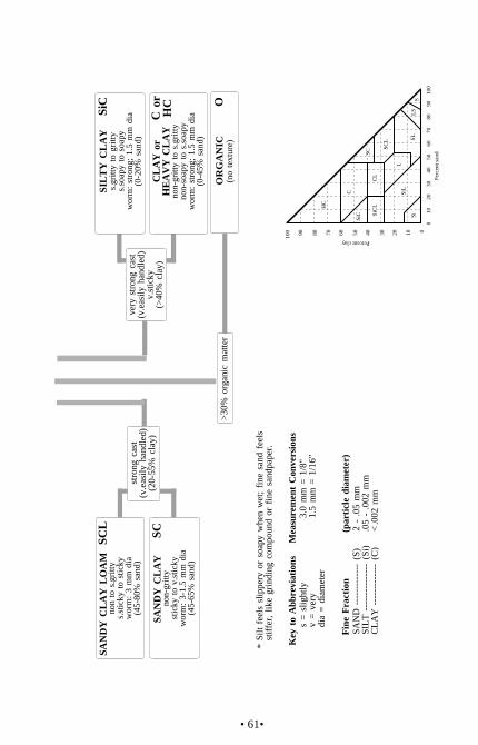
•61•
SA
ND
Y C
LAY
LO
AM
SC
LS
iCS
ILT
Y C
LAY
SA
ND
Y C
LAY
SC
OO
RG
AN
IC
C o
r H
CC
LAY
or
HE
AV
Y C
LAY
>30
% o
rgan
ic m
atte
r
non
to s
.grit
tys.
stic
ky t
o st
icky
wor
m:
3 m
m d
ia(4
5-80
% s
and)
s.gr
itty
to g
ritty
s.so
apy
to s
oapy
wor
m:
stro
ng;
1.5
mm
dia
(0-2
0% s
and)
non-
gritt
yst
icky
to
v.st
icky
wor
m:
3-1.
5 m
m d
ia(4
5-65
% s
and)
stro
ng c
ast
(v.e
asily
han
dled
)(2
0-55
% c
lay)
(no
text
ure)
non-
gritt
y to
s.g
ritty
non-
soap
y to
s.s
oapy
wor
m:
stro
ng;
1.5
mm
dia
(0-4
5% s
and)
Key
to
Abb
revi
atio
ns
Fin
e F
ract
ion
(par
ticle
dia
met
er)
Mea
sure
men
t C
onve
rsio
nss
= s
light
lyv
= v
ery
dia
= d
iam
eter
SA
ND
---
----
----
-- (
S)
2 -
.05
mm
SIL
T -
----
----
----
-- (
Si)
.05
- .0
02 m
mC
LAY
---
----
----
-- (
C)
<.0
02 m
mH
EA
VY
CLA
Y --
(HC
)>
60 %
cla
yLO
AM
---
----
----
- ( L
)m
ix o
f sa
nd,
silt,
and
cla
y
3.0
mm
= 1
/8"
1.5
mm
= 1
/16"
Silt
fee
ls s
lippe
ry o
r so
apy
whe
n w
et;
fine
sand
fee
ls
stiff
er,
like
grin
ding
com
poun
d or
fin
e sa
ndpa
per.
*
very
str
ong
cast
(v.e
asily
han
dled
)v.
stic
ky(>
40%
cla
y)
Percent clay
Per
cent
san
d
100 90 80 70 60 50 40 30 20 10 0
010
2030
4050
6070
8090
100
HC
C
SiC S
iCL
CL
SC
L
LS
iL
Si
SL
LSS
SC

•62•

3 VEGETATION
Contents
Vegetation Form ........................................................................ 3Field Procedure .......................................................................... 4Guidelines for Describing Vegetation..................................... 5
Vegetation Layers .................................................................. 5Species Lists ............................................................................ 6Unknown Species .................................................................. 6Plants Growing on Subdominant Substrates .................... 8Estimating Percent Cover .................................................... 8Recording Percent Cover ..................................................... 10Blank Columns on the Form ............................................... 10
Completing the Form ............................................................... 111. Species List ....................................................................... 112. Percent Cover by Layer ................................................ 113. Surveyor .......................................................................... 114. Plot Number .................................................................... 115. Page __ of __ ................................................................... 116. Trees .................................................................................. 117. Shrubs ............................................................................... 128. Herb Layer ...................................................................... 129. Moss, Lichen, and Seedling Layer ................................ 12
10. Additional Species ........................................................... 1211. Notes ................................................................................ 12
Appendix ..................................................................................... 123.1 Coding For Additional Information ............................ 13
Arboreal Lichen Loading ............................................ 13Available Forage .......................................................... 13Distribution Codes ...................................................... 13Utilization Ratings ....................................................... 14Coding for Vigour ....................................................... 14Phenology Codes: Vegetative Stages ...................... 15Phenology Codes: Generative Stages ..................... 16
Page
•2•
Tables3.1 List of low woody species and species of uncertain
life form assigned to the herb layer ............................. 73.2 Codes for subdominant substrates .............................. 83.3 Dimensions of various areas in a 400 m2 plot ............ 10
Figures3.1 Stratification of forest stands, shrubs, and trees ........ 63.2 Comparison charts for visual estimation of
foliage cover .................................................................... 93.3 An example of percent coverages in a plot, viewed
from above ...................................................................... 10

•3•
SP
P.
LIS
T
TR
EE
(A
)O
F
A1
A2
SH
RU
BS
NO
TE
S:
VEGETATION
%%H
ER
B L
AYE
R (
C)
TR
EE
S
SH
RU
B (
B)
HE
RB
(C
)M
OS
S /
LIC
HE
N (
D)
LAYE
R
PAG
ES
UR
VE
YO
R(S
)
B
B1
B2
B
B1
B2
AD
DIT
ION
AL
SP
EC
IES
MO
SS
/ LI
CH
EN
/ S
EE
DLI
NG
(D
)%
A3
A
CO
MP.
PAR
T.
% C
OV
ER
BY
LAY
ER
PLO
T
NO
.
FS
882
(3)
HR
E 9
8/511
7
1
6
2
89
34
5
10
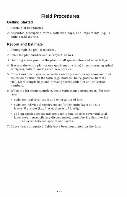
•4•
Field ProceduresGetting Started
1. Locate plot boundaries.
2 . Assemble description forms, collection bags, and implements (e.g., aknife, small shovel).
Record and Estimate
1. Photograph the plot, if required.
2. Enter the plot number and surveyors’ names.
3. Standing at one point in the plot, list all species observed in each layer.
4. Traverse the entire plot (or one quadrant at a time) in an increasing spiralor zig-zag pattern, noting each new species.
5. Collect unknown species, recording each by a temporary name and plotcollection number on the form (e.g., moss 01, hairy grass 02, herb 03,etc.). Mark sample bags and pressing sheets with plot and collectionnumbers.
6. When the list seems complete, begin estimating percent cover. For eachlayer:
• estimate total layer cover and enter at top of form;
• estimate individual species covers for the entire layer and sub-layers, if present (i.e., first A, then A1, A2, A3);
• add up species covers and compare to total species cover and totallayer cover; reconcile any discrepancies, remembering that overlap
can occur between species and layers.
7 . Check that all required fields have been completed on the form.

•5•
Guidelines for Describing Vegetation
Throughout the process of describing vegetation, observe the followingguidelines.
Vegetation LayersAll vegetation is assigned to one of the following layers. Criteria for A and Blayers and sub-layers are depicted in Figure 3.1.A. The tree layer includes all woody plants greater than 10 m tall. Three
sub-layers are recognized:A1 Dominant trees - includes the dominant (tallest) trees of the
main canopy, which may be veterans of one or more fires(previously classed as A0), or the tallest trees of the same ageclass as the main canopy; usually a minor portion of the standcomposition.
A2 Main tree canopy (codominant trees) - the main layer of treecover, composed of trees whose crowns form the upper layer offoliage; typically the major portion of the stand composition.
A3 Sub-canopy trees - includes trees greater than 10 m high that donot reach the main canopy; may form a distinct secondarycanopy; often a mixture of trees of various heights younger thanthose in the main canopy or may be suppressed trees of the sameage; includes “intermediate” and “overtopped” trees(terminology of MOF Resources Inventory Branch).
B. The shrub layer includes all woody plants less than 10 m tall, exceptlow (usually < 15 cm tall) woody or trailing plants which are consid-ered part of the herb layer (see Table 3.1). Established tree regenera-tion more than two years of age and less than 10 m in height isconsidered part of the shrub layer. Two sub-layers are recognized:B1 Tall shrub layer - includes all woody plants 2–10 m tall,
including shrubs and advance tree regeneration and trees inpoorly growing stands where the canopy is less than 10 m high.
B2 Low shrub layer - includes all woody plants less than 2 m high,except low (< 15 cm) woody or trailing plants (see Table 3.1);includes shrubs and established tree regeneration more than twoyears old and dwarfed or immature specimens of speciesnormally considered in the shrub category (e.g., young Vacciniummembranaceum, or dwarf alpine forms of normally taller shrubs).
C. The herb layer includes all herbaceous species, regardless of height, andsome low woody plants less than 15 cm tall (see Table 3.1).
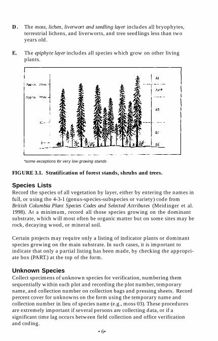
•6•
D. The moss, lichen, liverwort and seedling layer includes all bryophytes,terrestrial lichens, and liverworts, and tree seedlings less than twoyears old.
E. The epiphyte layer includes all species which grow on other livingplants.
Species ListsRecord the species of all vegetation by layer, either by entering the names infull, or using the 4-3-1 (genus-species-subspecies or variety) code fromBritish Columbia Plant Species Codes and Selected Attributes (Meidinger et al.1998). At a minimum, record all those species growing on the dominantsubstrate, which will most often be organic matter but on some sites may berock, decaying wood, or mineral soil.
Certain projects may require only a listing of indicator plants or dominantspecies growing on the main substrate. In such cases, it is important toindicate that only a partial listing has been made, by checking the appropri-ate box (PART.) at the top of the form.
Unknown SpeciesCollect specimens of unknown species for verification, numbering themsequentially within each plot and recording the plot number, temporaryname, and collection number on collection bags and pressing sheets. Recordpercent cover for unknowns on the form using the temporary name andcollection number in lieu of species name (e.g., moss 03). These proceduresare extremely important if several persons are collecting data, or if asignificant time lag occurs between field collection and office verificationand coding.
*some exceptions for very low growing stands
FIGURE 3.1. Stratification of forest stands, shrubs and trees.
*
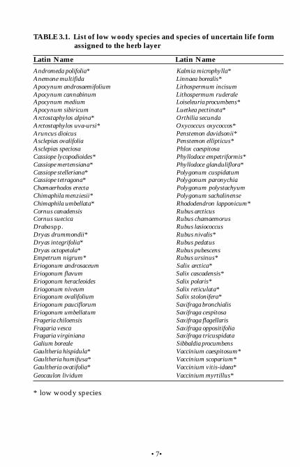
•7•
TABLE 3.1. List of low woody species and species of uncertain life formassigned to the herb layer
Andromeda polifolia* Kalmia microphylla*Anemone multifida Linnaea borealis*Apocynum androsaemifolium Lithospermum incisumApocynum cannabinum Lithospermum ruderaleApocynum medium Loiseleuria procumbens*Apocynum sibiricum Luetkea pectinata*Arctostaphylos alpina* Orthilia secundaArctostaphylos uva-ursi* Oxycoccus oxycoccos*Aruncus dioicus Penstemon davidsonii*Asclepias ovalifolia Penstemon ellipticus*Asclepias speciosa Phlox caespitosaCassiope lycopodioides* Phyllodoce empetriformis*Cassiope mertensiana* Phyllodoce glanduliflora*Cassiope stelleriana* Polygonum cuspidatumCassiope tetragona* Polygonum paronychiaChamaerhodos erecta Polygonum polystachyumChimaphila menziesii* Polygonum sachalinenseChimaphila umbellata* Rhododendron lapponicum*Cornus canadensis Rubus arcticusCornus suecica Rubus chamaemorusDraba spp. Rubus lasiococcusDryas drummondii* Rubus nivalis*Dryas integrifolia* Rubus pedatusDryas octopetala* Rubus pubescensEmpetrum nigrum* Rubus ursinus*Eriogonum androsaceum Salix arctica*Eriogonum flavum Salix cascadensis*Eriogonum heracleoides Salix polaris*Eriogonum niveum Salix reticulata*Eriogonum ovalifolium Salix stolonifera*Eriogonum pauciflorum Saxifraga bronchialisEriogonum umbellatum Saxifraga cespitosaFrageria chiloensis Saxifraga flagellarisFragaria vesca Saxifraga oppositifoliaFragaria virginiana Saxifraga tricuspidataGalium boreale Sibbaldia procumbensGaultheria hispidula* Vaccinium caespitosum*Gaultheria humifusa* Vaccinium scoparium*Gaultheria ovatifolia* Vaccinium vitis-idaea*Geocaulon lividum Vaccinium myrtillus*
* low woody species
Latin Name Latin Name

•8•
Plants Growing on Subdominant SubstratesWhere the objectives of a study or the features of a particular site warrantcollecting data for plants growing on substrates other than the dominantsubstrate, list these under “Additional Species” on the form. Identify thelayer to which the plant belongs (A–E) and the type of substrate using thecodes in Table 3.2. Label the top of the blank column used to record the typeof substrate as "SS" (subdominant substrate).
TABLE 3.2. Codes for subdominant substrates
Estimating Percent CoverIn most surveys, only those species growing on the dominant substrate areincluded in estimates. Percent cover is estimated as the percentage of theground surface covered when the crowns are projected vertically. Followthe outside perimeter of the projected crown. For the tree layer, distinctholes in the canopy should be subtracted from the estimate. For otherlayers, small gaps that are not fully covered can be ignored.
• Viewing the layer obliquely, rather than vertically, can result in anover-estimation.
• Avoid biasing estimates because of crown density.
• For species with high cover values, mentally move the plants to acorner of the plot to estimate if they represent one-quarter, one-third,or one-half, or more of the plot.
• For species that almost cover the plot, mentally move them togetherand estimate how much of the area is not covered by the plants.
• For species with low cover, try making estimates for subsections in eachquarter of the plot.
• Equating percent cover with equivalent dimensions relative to plot areacan be very helpful (Table 3.3). For several small scattered areas ofcoverage, think about the area covered by 1% (2 x 2 m in a 400 m2
plot), or 0.1% (63 x 63 cm), and add up the total number of areas ofcover that are roughly equivalent to these dimensions.
Code DescriptionA Aquatic; where water is the subdominant substrateL Cobbles, stones, or bedrock outcrops (epiliths)O Organic matter (e.g., plants growing on patches of organic matter on
a talus slope where the dominant substrate is rock)S Bare soil (episols)X Dead wood (epixyles)

•9•
FIGURE 3.2. Comparison charts for visual estimation of foliage cover.
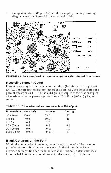
•10•
FIGURE 3.3. An example of percent coverages in a plot, viewed from above.
• Comparison charts (Figure 3.2) and the example percentage coveragediagram shown in Figure 3.3 are other useful aids.
Recording Percent CoverPercent cover may be entered in whole numbers (1–100), tenths of a percent(0.1–0.9), hundredths of a percent (recorded as 1H–9H), and thousandths of apercent (recorded as 1T– 9T). Table 3.3 gives examples of the relationship ofdimensional area to percentage area, for a 20 x 20 m (400 m2) plot, andcoding.
TABLE 3.3. Dimensions of various areas in a 400 m2 plot
Dimensions Area (m2) % cover Coding
10 x 10 m 100.0 25.0 255 x 8 m 40.0 10.0 102 x 2 m 4.0 1.0 163 x 63 cm 0.4 0.1 0.120 x 20 cm 0.04 0.01 1H6.3 x 6.3 cm 0.004 0.001 1T
Blank Columns on the FormWithin the main body of the form, immediately to the left of the columnsprovided for recording percent cover, two blank columns have beenprovided for recording additional information. Suggested items that maybe recorded here include subdominant substrates (SS), distribution

•11•
codes (DC), plant vigour ratings (VI), phenology (PV or PG), utilization(UT), estimates of available forage (AF), and arboreal lichen loading(LL). Codes for these items are provided in Appendix 3.1. Enter a two-letter abbreviation for the type of data at the top of each column used.For types of data other than those listed here, explain under Item 11,"Notes."
Completing the FormNumbered items below refer to circled numbers on the Vegetation Descrip-tion Form shown at the beginning of this section. A recommendedsequence for completing the form is described under "Field Procedure."
1. Species ListCertain projects may require a listing of dominant or indicator species only.Check the appropriate box to indicate whether an attempt has been madeto record a complete listing of all species on the dominant substrate("Comp."), or if only a partial list has been made ("Part.").
2. Percent Cover by LayerAfter all species have been listed, enter the total percent cover by layer (seedescriptions of layers and instructions for estimating and recording percentcover at the beginning of this section). Note that because of overlaps the sumof the percent cover values for all species within each layer may be greaterthan the total layer coverage.
3. Surveyor(s)Record the first initial and last name of the person(s) who described thevegetation.
4. Plot NumberRecord plot number from the Site Description Form.
5. Page __ of __If more than one page is required, enter the number as a total and numbereach page.
6. TreesEstimate percent cover for each tree species by sub-layer and layer (A1, A2,A3, A, B1, B2, B). If trees in A1 are veterans, record this under Item 11,"Notes." For each of the A and B layers, the total percent coverage for aspecies will often be less than the sum of the covers for each of the sub-layers, due to crown overlap.

•12•
7. ShrubsEstimate percent cover for each shrub species by sub-layer (B1 and B2),and as a total for the species (B). The total percent coverage of a specieswill often be less than the sum of the two sub-layer values due to overlap offoliage.
8. Herb LayerEstimate percent cover for each species in the herb (C) layer.
9. Moss, Lichen, and Seedling LayerEstimate percent cover for each moss, lichen, and seedling species in thislayer (D).
10. Additional SpeciesUse these lines to list species from the E layer (epiphytes), additional speciesfrom any other layer if there has been insufficient space elsewhere on theform, and species growing on subdominant substrates.
11. NotesUse this space to record important features not described elsewhere, or forexplanatory notes keyed to other entries on the vegetation form.

•13•
APPENDIX 3.1 Coding for Additional Information
Arboreal Lichen Loading (LL)If a "Tree Attributes for Wildlife" form is not required, a general assessmentof lichen loading can be recorded by tree species on the vegetation descrip-tion form. Assess standing live and dead trees for lichen loading on thebranches within 4.5 m of the ground or root collar. Assign an overall rating(0–5) by species by comparing with photos in Estimating the Abundance ofAboreal Forage Lichens (Armleder et al. 1992). A value of 0 indicates nolichens. If trees have lichens, but none are below the 4.5 m mark, rate as zero.
Available Forage (AF)The amount of available forage may be estimated or measured in g/m2 andrecorded by species in one of the blank columns. If estimated for groups ofspecies, such as palatable forbs, grasses, browse species, undesirable species,etc., record under item 11, "Notes." Also indicate whether forage wasmeasured or estimated and note the method of determining weight (i.e.,estimated green, air-dried, or oven-dried).
Distribution Codes (DC)The spatial distribution pattern of individuals of each species is describedusing the following codes:
Description
Rare individual, single occurrence
A few sporadically occurringindividuals
A single patch or clump of a species
Several sporadically occurringindividuals
A few patches or clumps of aspecies
Several well-spaced patches orclumps
Continuous uniform occurrence ofwell-spaced individuals
Code
1
2
3
4
5
6
7
No. plantsa in 400 m2
1
2–5
1 patch (< 25% of plot)
> 6
2–5 patches, each < 25% ofplot
> 6 patches, each < 25% ofplot
many
(over)

•14•
Utilization Ratings (UT)Coding for utilization (present use) of browse and forage species is asfollows:
Coding for Vigour (VI)Plant vigour is described using the following codes:
Code
8
9
Description
Continuous occurrence of aspecies with a few gaps in thedistribution
Continuous dense occurrence of aspecies
No. plantsa in 400 m2
many
many
Code % utilization Description
0 0 Nil1 1-15 Slight2 16-36 Light3 36-65 Moderate4 66-80 Heavy5 > 80 Extreme
Code Description
0 Species dead1 Vigour poor2 Vigour fair3 Vigour good4 Vigour excellent
a guidelines for low shrubs, herbs, and mosses
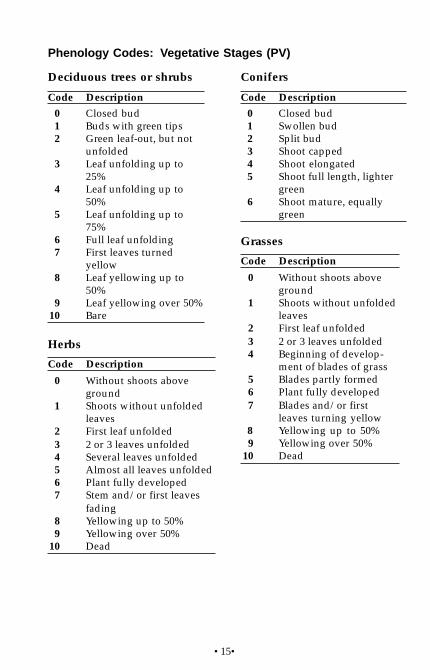
•15•
Phenology Codes: Vegetative Stages (PV)
Deciduous trees or shrubs
Code Description
0 Closed bud1 Buds with green tips2 Green leaf-out, but not
unfolded3 Leaf unfolding up to
25%4 Leaf unfolding up to
50%5 Leaf unfolding up to
75%6 Full leaf unfolding7 First leaves turned
yellow8 Leaf yellowing up to
50%9 Leaf yellowing over 50%
10 Bare
Conifers
Code Description
0 Closed bud1 Swollen bud2 Split bud3 Shoot capped4 Shoot elongated5 Shoot full length, lighter
green6 Shoot mature, equally
green
Herbs
Code Description
0 Without shoots aboveground
1 Shoots without unfoldedleaves
2 First leaf unfolded3 2 or 3 leaves unfolded4 Several leaves unfolded5 Almost all leaves unfolded6 Plant fully developed7 Stem and/or first leaves
fading8 Yellowing up to 50%9 Yellowing over 50%
10 Dead
Grasses
Code Description
0 Without shoots aboveground
1 Shoots without unfoldedleaves
2 First leaf unfolded3 2 or 3 leaves unfolded4 Beginning of develop-
ment of blades of grass5 Blades partly formed6 Plant fully developed7 Blades and/or first
leaves turning yellow8 Yellowing up to 50%9 Yellowing over 50%
10 Dead
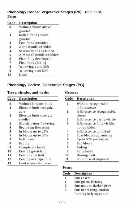
•16•
Grasses
Code Description
0 Without recognizableinflorescence
1 Inflorescence recognizable,closed
2 Inflorescence partly visible3 Inflorescence fully visible,
not unfolded4 Inflorescence unfolded5 First blooms pollenizing6 Up to 50% pollenized7 Full bloom8 Fading9 Fully faded
10 Bearing fruit11 Fruit or seed dispersal
Ferns
Code Description0 Without shoots above
ground1 Rolled fronds above
ground2 First frond unfolded3 2 or 3 fronds unfolded4 Several fronds unfolded5 Almost all fronds unfolded6 Plant fully developed7 First fronds fading8 Yellowing up to 50%9 Yellowing over 50%
10 Dead
Phenology Codes: Vegetative Stages (PV) (continued)
Phenology Codes: Generative Stages (PG)
Trees, shrubs, and herbs
Code Description
0 Without blossom buds1 Blossom buds recogniz-
able2 Blossom buds strongly
swollen3 Shortly before flowering4 Beginning flowering5 In bloom up to 25%6 In bloom up to 50%7 Full bloom8 Fading9 Completely faded
10 Bearing green fruit11 Bearing ripe fruit12 Bearing overripe fruit13 Fruit or seed dispersal
Ferns
Code Description0 Sori absent1 Sori green, forming2 Sori mature, darker, drier3 Sori depressing, strobili
forming in lycopodium
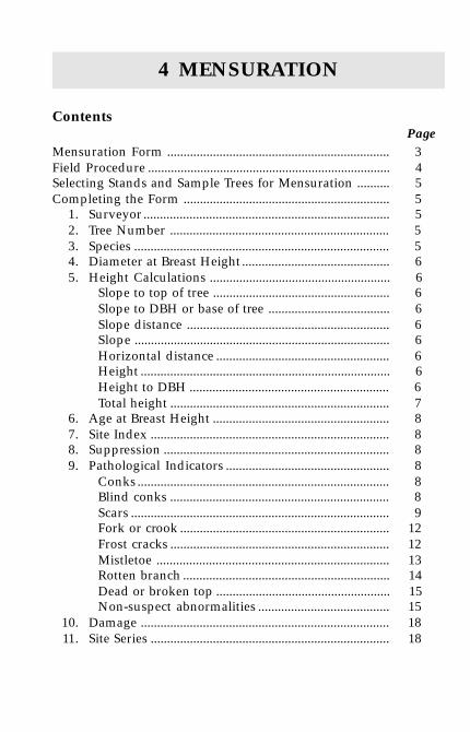
Contents
Mensuration Form .................................................................... 3Field Procedure .......................................................................... 4Selecting Stands and Sample Trees for Mensuration .......... 5Completing the Form ............................................................... 5
1. Surveyor ........................................................................... 52. Tree Number ................................................................... 53. Species .............................................................................. 54. Diameter at Breast Height ............................................. 65. Height Calculations ....................................................... 6
Slope to top of tree ...................................................... 6Slope to DBH or base of tree ..................................... 6Slope distance .............................................................. 6Slope .............................................................................. 6Horizontal distance ..................................................... 6Height ............................................................................ 6Height to DBH ............................................................. 6Total height ................................................................... 7
6. Age at Breast Height ...................................................... 87. Site Index ......................................................................... 88. Suppression ..................................................................... 89. Pathological Indicators .................................................. 8
Conks............................................................................. 8Blind conks ................................................................... 8Scars ............................................................................... 9Fork or crook ................................................................ 12Frost cracks ................................................................... 12Mistletoe ....................................................................... 13Rotten branch ............................................................... 14Dead or broken top ..................................................... 15Non-suspect abnormalities ........................................ 15
10. Damage ............................................................................ 1811. Site Series ......................................................................... 18
4 MENSURATION
Page
•2•
Appendices4.1 Tree species codes ........................................................... 194.2 Damage agent codes ...................................................... 22
Tables4.1 Slope distance factors .................................................... 74.2 Defect location codes ..................................................... 8
Figures4.1 Blind conk and sound knot, on a standing tree and in
cross-section .................................................................... 94.2 Appearance of scars that are old or freshly healed .. 104.3 Appearance of scars with light or heavy damage .... 114.4 Appearance of cankers caused by fungi .................... 114.5 Appearance of scars caused by rock slides or
falling rock....................................................................... 114.6 Appearance of different forms of forks and crooks . 124.7 Appearance of frost cracks on standing tree and
in cross-section................................................................ 134.8 Examples of mistletoe infection................................... 134.9 How to determine if mistletoe infection causes tree
to be suspect ................................................................... 144.10 How to determine if rotten branches are a probable
indicator of decay........................................................... 14
Page

•3•
ME
NS
UR
ATIO
N F
OR
MS
UR
VE
YO
R(S
):
TREE#S
PP.
DB
HT
OP
BO
T.S
DS
L.H
DH
T.
HT.
TO
DB
H
TOTA
LH
T.B
HA
GE
SI
SU
P.
BL. CONK
SCAR.
CONK
F. OR C.
F. CRACK
MISTLE.
R. BRAN.
D. OR B.TOP
TY
PE
SE
V.
DA
MA
GE
SIT
ES
ER
IES
HE
IGH
T C
ALC
ULA
TIO
NS
MENSURATION
FS
882
(4)
HR
E 9
8/5
NO
TE
ST
RE
E D
IAM
ET
ER
TA
LLY
TR
EE
#T
RE
E #
SP
P.D
BH
SP
P.D
BH11
10
1
98
76
52
34

•4•
Field Procedure
Getting Started
1. Establish plot boundaries.
2. Traverse the plot systematically to identify candidate sample treesaccording to project objectives. If largest diameter trees are beingsampled, use Tree Diameter Tally to assist in selection.
3. When numbering trees, start with the tree closest to due north of plotcentre and proceed in a clockwise direction.
Measure and Record
1. Enter the name(s) of persons collecting mensuration data.
2. Record tree numbers and species of sample trees.
3. Examine each tree for evidence of suppression, pathological indicators,and pests or injury. If present, and if determining the site index is aprimary objective of the project, select a different sample that is free ofdefects (if possible). If site index is not a primary objective, or noalternate defect-free trees exist, retain the sample and enter coding asappropriate.
4. Determine and record diameters and age at breast height. If age is to bedetermined later, place the collected core in a labelled straw.
5. Determine and record measurements for height calculations.
6. Calculate height, total height, and site index (or leave blank andcalculate using SiteTools software and the data entry program VENUS).
7. If the site is variable, identify the site series code for the area aroundeach tree, in consultation with other surveyors.
8. Check that all the required information has been collected and noted onthe form. Strike through any fields that were not assessed.

•5•
Selecting Stands and SampleTrees for Mensuration
Stand selection criteria will depend entirely on project objectives. If the datais being collected to determine site index, stands should have the followingcharacteristics:
• even-aged (preferably 20–150 years of age)
• dominated by one tree species (or target species > 60% of basal area)
• moderately dense
• ecologically uniform site of at least 400 m2
When determining site index is not a primary objective, select the two orthree largest diameter trees of each species for mensuration. If the data isbeing collected to determine site index, collect mensuration data on “top-height” trees that meet the following criteria:
• 100 largest diameter trees per hectare (largest 4 per 400 m2 plot)
• dominant or co-dominant
• not wolf, open grown, or veteran
• straight-stemmed, free of disease, damage, and breakage
• free of suppression (above breast height)
• vigorous, with full crowns
Completing the Form
Numbered items below refer to circled numbers on the Mensuration formshown at the beginning of this section. A recommended sequence forcompleting the form is described under “Field Procedure.”
1. SurveyorEnter the first initial and last name of the person(s) collecting mensurationdata.
2. Tree NumberAssign numbers sequentially to each tree sampled. Start with the tree closestto due north of plot centre and proceed clockwise. Numbers may be paintedor tagged on trees.
3. SpeciesIdentify tree species using the codes given in Appendix 4.1.

•6•
4. Diameter at Breast HeightRecord DBH (diameter at breast height) to the nearest 0.1 cm. Measure at1.3 m above the point of germination. On slopes, measure from the high sideof the root collar.
5. Height CalculationsRecord the following measurements: heights and distances in metres andslopes in percent. Tree height can be calculated in the field using equationsand tables provided, or automatically using the data entry program“VENUS.”
Slope to top of tree (TOP):Enter the percent slope reading to the top of the tree, showing the sign(usually “+”). If a reading greater than 100% is obtained, move further fromthe tree, or upslope.
Slope to DBH or base of tree (BOT):Enter the percent slope reading to DBH, or to the base of the tree, or tolowest visible point, including the sign (“+” or “–”). The maximum allow-able is 100%.
Slope distance (SD):Enter the distance (in metres, to one decimal) from the observer to the centreof the tree trunk, usually at breast height.
Slope (SL):Enter the slope gradient between the observer and the tree at breast height(the slope of the measuring tape used to determine slope distance). Thisvalue is used in height calculations done by “VENUS.”
Horizontal distance (HD):Calculate this by multiplying slope distance (SD) by a slope distance factorfrom Table 4.1. The slope percent column in this table refers to the slopegradient measurement Slope (SL).
Height (HT):Enter the height (m) of the measured part of the tree to one decimal,calculated as follows:HT = [(TOP – BOT) × HD] ÷ 100
Height to DBH (HT TO DBH):If the BOT reading was not taken at the base of the tree, record the height atwhich it was taken. This is usually DBH, but can be another value. Enter“0” if taken at the base of tree.

•7•
% slope Factor % slope Factor % slope Factor
10 .995 36 .941 62 .84911 .994 37 .938 63 .84612 .993 38 .935 64 .84213 .992 39 .932 65 .83814 .990 40 .928 66 .83415 .989 41 .925 67 .83016 .987 42 .922 68 .82717 .986 43 .919 69 .82318 .984 44 .915 70a .81919 .982 45 .912 75 .80020 .980 46 .908 80 .78121 .979 47 .905 85 .76222 .977 48 .902 90 .74323 .974 49 .898 95 .72524 .972 50 .894 100 .70725 .970 51 .890 105 .69026 .968 52 .887 110 .67327 .965 53 .883 115 .65628 .963 54 .880 120 .64029 .960 55 .876 125 .62530 .958 56 .872 130 .61031 .955 57 .868 135 .59532 .952 58 .865 140 .58133 .950 59 .861 150 .55534 .941 60 .85735 .944 61 .853
a Interpolate for slopes between 70 and 150%.
Total height (TOTAL HT) :The total height of the tree = HT + HT TO DBH
Note the following example calculation:TOP = +62, BOT = –24, TOP – BOT = 62–(–24) = 86SD = 20.5 m, SL = 23%, slope distance factor (from table) = 0.974HD = SD × slope distance factor = 20.5 × 0.974 = 20.0HT = [(TOP – BOT) × HD] ÷ 100 = (86 × 20.0) ÷ 100 = 17.2 mHT TO DBH = 1.3 mTotal height = HT + HT TO DBH = 17.2 + 1.3 = 18.5 m
TABLE 4.1. Slope distance factors
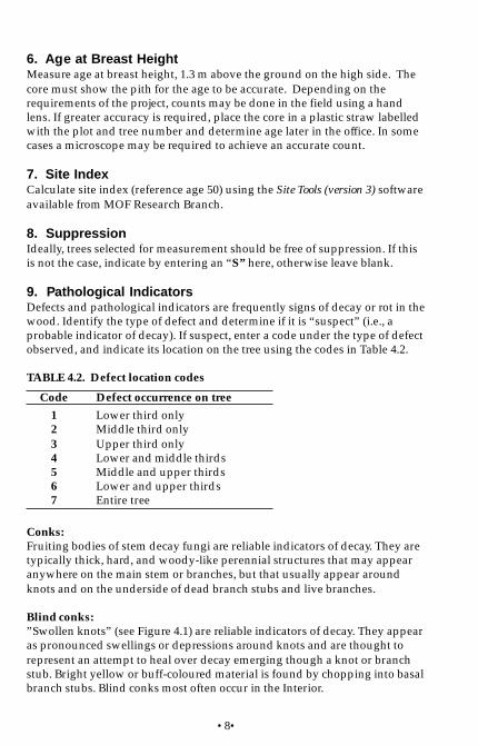
•8•
6. Age at Breast HeightMeasure age at breast height, 1.3 m above the ground on the high side. Thecore must show the pith for the age to be accurate. Depending on therequirements of the project, counts may be done in the field using a handlens. If greater accuracy is required, place the core in a plastic straw labelledwith the plot and tree number and determine age later in the office. In somecases a microscope may be required to achieve an accurate count.
7. Site IndexCalculate site index (reference age 50) using the Site Tools (version 3) softwareavailable from MOF Research Branch.
8. SuppressionIdeally, trees selected for measurement should be free of suppression. If thisis not the case, indicate by entering an “S” here, otherwise leave blank.
9. Pathological IndicatorsDefects and pathological indicators are frequently signs of decay or rot in thewood. Identify the type of defect and determine if it is “suspect” (i.e., aprobable indicator of decay). If suspect, enter a code under the type of defectobserved, and indicate its location on the tree using the codes in Table 4.2.
Code Defect occurrence on tree
1 Lower third only2 Middle third only3 Upper third only4 Lower and middle thirds5 Middle and upper thirds6 Lower and upper thirds7 Entire tree
TABLE 4.2. Defect location codes
Conks:Fruiting bodies of stem decay fungi are reliable indicators of decay. They aretypically thick, hard, and woody-like perennial structures that may appearanywhere on the main stem or branches, but that usually appear aroundknots and on the underside of dead branch stubs and live branches.
Blind conks:”Swollen knots” (see Figure 4.1) are reliable indicators of decay. They appearas pronounced swellings or depressions around knots and are thought torepresent an attempt to heal over decay emerging though a knot or branchstub. Bright yellow or buff-coloured material is found by chopping into basalbranch stubs. Blind conks most often occur in the Interior.

•9•
Scars:Scars result from past injuries caused by external forces that have damagedthe cambium or heartwood, exposing the tree to wood decay fungi. Thesescars are considered suspect if located on the main stem or root collar, unlessthey are of recent origin (Figures 4.2 and 4.3).Scars may be open or closed. Open scars are areas of exposed wood ofvarying size and shape from severe damage caused by fire, lightning,logging, machinery, etc. Closed scars may appear healed over, with slight topronounced indentations of the bark, or there may be pronounced scar tissueor callous growth, often with abundant resin flow.Several common types of scars are described below.Fire scars – may appear as indentations, open catfaces, or hollowing of thetrunk; usually confined to base of trunk.Lightning scars – extensive damage to the trunks and tops of trees; strips oftorn wood typically observed, often extending the entire length of the tree ina spiral.Falling-tree scars – the fallen tree generally found against or near thescarred tree.Logging or other machinery scars – selective cutting operations may causeextensive damage; usually on the base of the trunk, or the upper portion ofthe trunk if caused by rigging.Old blazing – frequent entry points for wood-rotting fungi; do not recordrecent blazing.
FIGURE 4.1. Blind conk and sound knot, on a standing tree and in cross-section.

•10•
FIGURE 4.2. Appearance of scars that are old or freshly healed.
Scars caused by breakage – scars on trunks from the breakage of livebranches or secondary leaders; breakage caused by high winds, heavy snow,or branches falling from adjacent trees.Animal or bird scars – for example, woodpeckers can make large, deepholes in the trunk; bears, deer, moose, and elk may remove areas of bark andcambium; scars can be caused by bear claws and gnawing by beavers orother rodents.Cankers caused by fungi – results in the death of localized areas of bark andcambium (Figure 4.4); dead bark is sloughed off, exposing underlying wood;usually evidence of repeated callous growth; may be mistaken for “mechani-cal” scars; usually flattened, elongated, and of irregular shape; exposedwood often stained and impregnated with resin; fruiting bodies of thefungus may be visible.Scars caused by rock slides or falling rock – usually confined to base oftrunk, however falling rock sometimes causes scars much higher on stembecause of high snow levels or rocks bouncing; usually occur on the upslopeside (Figure 4.5).
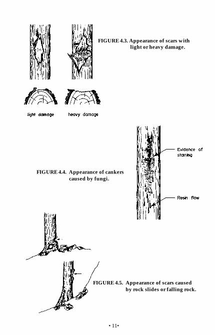
•11•
FIGURE 4.3. Appearance of scars with light or heavy damage.
FIGURE 4.4. Appearance of cankers caused by fungi.
FIGURE 4.5. Appearance of scars caused by rock slides or falling rock.

•12•
Fork or crook (F or C):Forks or crooks that develop after an early injury to the top of the tree arereliable indicators of decay (Figure 4.6). The following are not consideredforks: candelabra branches; natural branching in deciduous trees; small,sharply angled branches or spikes, unless associated with a noticeable offsetor diameter change at the location; flattening of tree tops caused by wind orphysiological conditions where no terminal leaders are evident.
FIGURE 4.6. Appearance of different forms of forks and crooks.
Frost cracks (F. Crack):Frost cracks are caused by uneven expansion of moisture in the treefollowing a sudden and pronounced drop in temperature. They result indeep radial splitting of the trunk and are considered suspect. Usuallyoriginating at the base of the trunk, frost cracks may extend many metres upthe tree. These cracks are often re-opened by wind stresses or low tempera-tures; repeated healing of the wood produces considerable callous tissue,giving the wound a pronounced ribbed appearance (Figure 4.7).
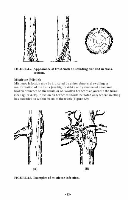
•13•
FIGURE 4.8. Examples of mistletoe infection.
FIGURE 4.7. Appearance of frost crack on standing tree and in cross- section.
Mistletoe (Mistle):Mistletoe infection may be indicated by either abnormal swelling ormalformation of the trunk (see Figure 4.8A), or by clusters of dead andbroken branches on the trunk, or on swollen branches adjacent to the trunk(see Figure 4.8B). Infection on branches should be noted only where swellinghas extended to within 30 cm of the trunk (Figure 4.9).
(A) (B)

•14•
FIGURE 4.9. How to determine if mistletoe infection causes tree to be suspect.
Rotten Branch (R. Bran.):Large, rotten branches, typically on old-growth trees often indicate decay.Note only those branches that are greater than or equal to 10 cm in diameterat the base and that are clearly rotten (usually on overmature trees) (seeFigure 4.10A). Do not include small, dead branches typically just below thelive crown or on the lower trunk of open-growntrees (see Figure 4.10B).
FIGURE 4.10. How to determine if rotten branches are a probable indicator of decay.
(A) (B)
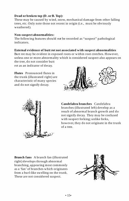
•15•
Dead or broken top (D. or B. Top):These may be caused by wind, snow, mechanical damage from other fallingtrees, etc. Only note those not recent in origin (i.e., must be obviouslyweathered).
Non-suspect abnormalities:The following features should not be recorded as “suspect” pathologicalindicators.
External evidence of butt rot not associated with suspect abnormalitiesButt rot may be evident in exposed roots or within root crotches. However,unless one or more abnormality which is considered suspect also appears onthe tree, do not consider buttrot as an indicator of decay.
Flutes Pronounced flutes inthe trunk (illustrated right) arecharacteristic of many speciesand do not signify decay.
Candelabra branches Candelabrabranches (illustrated left) develop as aresult of abnormal branch growth and donot signify decay. They may be confusedwith suspect forking; unlike forks,however, they do not originate in the trunkof a tree.
Branch fans A branch fan (illustratedright) develops through abnormalbranching, appearing most commonlyas a ‘fan’ of branches which originatesfrom a burl-like swelling on the trunk.These are not considered suspect.

•16•
Black knots Black knots (illustrated right) frequentlydevelop around unhealed knots and wounds. A superfi-cial saprophytic fungus feeding on exuded sap causes theblackness. These do not signify decay.
Burls and galls Burls and galls(illustrated left) develop fromabnormal cell growth in trees.Although formidable in appear-ance, they do not signify decay.
Sweep Sweep refers to a slight curvature or distortionof the trunk (illustrated right). This does not indicatedecay.
Exposed roots Exposed roots and buttress roots (shown below) do notsignify decay unless scarring is present above the point of germination.

•17•
Spiral grain Spiral grain is a growth characteristic of some trees and doesnot signify decay.
Dry side Dry side results from the death of the cambium through bruisingby other trees or other physiological causes. It appears as a narrow to widestrip or small localized area on the side of a tree, with the bark oftenremaining intact over the dead areas. Does not signify the presence of decay.
Sapsucker holes Sapsucker holes are superficial and do not signify decay.Do not confuse with the deeper scarring of woodpeckers.
Insect borings Borings by bark beetles or by other insects do not signifydecay and are non-suspect.

•18•
10. DamageSpecify the type of damage agent and severity of effect on the tree. Damageagents may include insects, diseases, wildlife, competing vegetation, orabiotic agents. If more than one type occurs on the same tree, record the mostdamaging one.
Type of Damage (Type):Specify the type of damage agent using codes listed in Appendix 4.2.
Severity of Damage (Sev.):Rate the severity of the effect on the tree. Either assess subjectively using thefollowing codes or leave blank (severity is difficult to assess withouttraining).
L = LowM = ModerateS = SevereP = Past attacks
11. Site SeriesIf the site is variable, enter the site series code for the area in a 4 m radiusaround the tree.
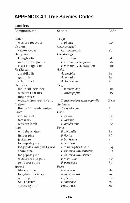
•19•
APPENDIX 4.1 Tree Species Codes
ConifersCommon name Species Code
Cedar Thujawestern redcedar T. plicata Cw
Cypress Chamaecyparisyellow-cedar C. nootkatensis Yc
Douglas-fir PseudotsugaDouglas-fir P. menziesii Fdinterior Douglas-fir P. menziesii var. glauca Fdicoast Douglas-fir P. menziesii var. menziesii Fdc
Fir (Balsam) Abiesamabilis fir A. amabilis Bagrand fir A. grandis Bgsubalpine fir A. lasiocarpa Bl
Hemlock Tsugamountain hemlock T. mertensiana Hmwestern hemlock T. heterophylla Hw
mountain x western hemlock hybrid T. mertensiana x heterophylla HxmJuniper Juniperus
Rocky Mountain juniper J. scopulorum JrLarch Larix
alpine larch L. lyallii Latamarack L. laricina Ltwestern larch L. occidentalis Lw
Pine Pinuswhitebark pine P. albicaulis Palimber pine P. flexilis Pfjack pine P. banksiana Pjlodgepole pine P. contorta Pllodgepole x jack pine hybrid P. x murraybanksiana Pxjshore pine P. contorta var. contorta Plclodgepole pine P. contorta var. latifolia Pliwestern white pine P. monticola Pwponderosa pine P. ponderosa Py
Spruce Piceablack spruce P. mariana SbEngelmann spruce P. engelmannii Sewhite spruce P. glauca SwSitka spruce P. sitchensis Ssspruce hybrid Picea cross Sx
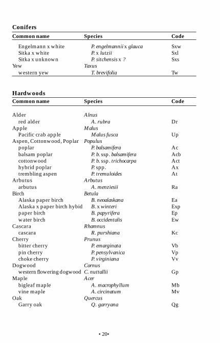
•20•
ConifersCommon name Species Code
Engelmann x white P. engelmannii x glauca SxwSitka x white P. x lutzii SxlSitka x unknown P. sitchensis x ? Sxs
Yew Taxuswestern yew T. brevifolia Tw
HardwoodsCommon name Species Code
Alder Alnusred alder A. rubra Dr
Apple MalusPacific crab apple Malus fusca Up
Aspen, Cottonwood, Poplar Populuspoplar P. balsamifera Acbalsam poplar P. b. ssp. balsamifera Acbcottonwood P. b. ssp. trichocarpa Acthybrid poplar P. spp. Axtrembling aspen P. tremuloides At
Arbutus Arbutusarbutus A. menziesii Ra
Birch BetulaAlaska paper birch B. neoalaskana EaAlaska x paper birch hybid B. x winteri Exppaper birch B. papyrifera Epwater birch B. occidentalis Ew
Cascara Rhamnuscascara R. purshiana Kc
Cherry Prunusbitter cherry P. emarginata Vbpin cherry P. pensylvanica Vpchoke cherry P. virginiana Vv
Dogwood Cornuswestern flowering dogwood C. nuttallii Gp
Maple Acerbigleaf maple A. macrophyllum Mbvine maple A. circinatum Mv
Oak QuercusGarry oak Q. garryana Qg

•21•
Willow Salixpeach-leaf willow S. amygdaloides WaBebb’s willow S. bebbiana Wbpussy willow S. discolor WdPacific willow S. lucida WpScouler’s willow S. scouleriana WsSitka willow S. sitchensis Wt
OthersCommon name Species Code
UnknownUnknown conifer XcUnknown hardwood Xh
Other tree, not on listOther conifer ZcOther hardwood Zh
Exotics1
Common name Species Code
Apple Malusapple Malus pumila Ua
Aspen, Cottonwood or PoplarPopulus*southern cottonwood P. deltoides Ad
Birch BetulaEuropean birch B. pendula Eesilver birch B. pubescens Es
Cherry Prunussweet cherry P. avium Vs
Cypress Chamaecyparis*Port Orford-cedar C. lawsoniana Yp
Fir (Balsam) Abies*balsam fir A. balsamea Bbnoble fir A. procera Bp*Shasta red fir A. magnifica var. shastensis Bm*white fir A. concolor Bc
Larch Larix*Siberian larch L. siberica Ls
Maple Acerbox elder A. negundo Me
HardwoodsCommon name Species Code

•22•
Exotics1
Common name Species Code
*Norway maple A. platanoides Mn*Sycamore maple A. pseudoplatanus Ms
Other exotics*incense-cedar Calocedrus decurrens Oa*giant sequoia Sequoiadendron giganteum Ob*coast redwood Sequoia sempervirens OcEuropean mountain-ash Sorbus aucuparia OdSiberian elm Ulmus pumila Oecommon pear Pyrus communis OfOregon ash Fraxinus latifolia Og
Pine Pinus*Monterey pine P. radiata Pm*red pine P. resinosa Pr*sugar pine P. lambertiana Ps
Oak Quercus*English oak Q. robur Qe
Spruce Picea*Norway spruce P. abies Sn
1 (*) Introduced species not known to occur on Crown Land, but requiring a code fordatabase purposes, are indicated with an asterisk.
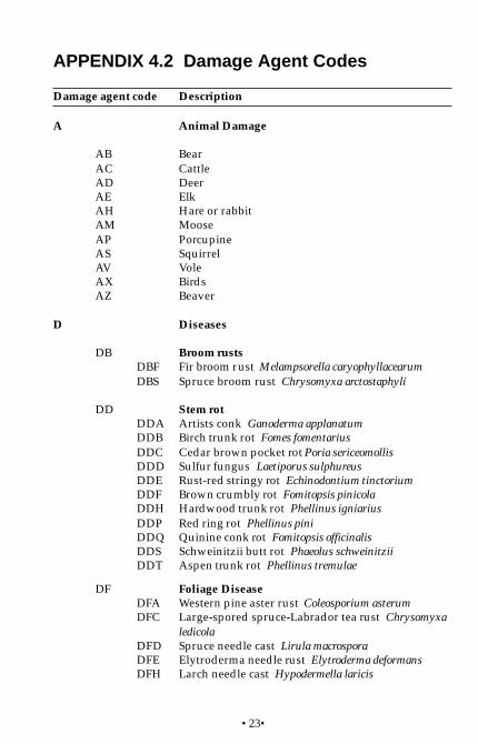
•23•
APPENDIX 4.2 Damage Agent Codes
Damage agent code Description
A Animal Damage
AB BearAC CattleAD DeerAE ElkAH Hare or rabbitAM MooseAP PorcupineAS SquirrelAV VoleAX BirdsAZ Beaver
D Diseases
DB Broom rustsDBF Fir broom rust Melampsorella caryophyllacearumDBS Spruce broom rust Chrysomyxa arctostaphyli
DD Stem rotDDA Artists conk Ganoderma applanatumDDB Birch trunk rot Fomes fomentariusDDC Cedar brown pocket rot Poria sericeomollisDDD Sulfur fungus Laetiporus sulphureusDDE Rust-red stringy rot Echinodontium tinctoriumDDF Brown crumbly rot Fomitopsis pinicolaDDH Hardwood trunk rot Phellinus igniariusDDP Red ring rot Phellinus piniDDQ Quinine conk rot Fomitopsis officinalisDDS Schweinitzii butt rot Phaeolus schweinitziiDDT Aspen trunk rot Phellinus tremulae
DF Foliage DiseaseDFA Western pine aster rust Coleosporium asterumDFC Large-spored spruce-Labrador tea rust Chrysomyxa
ledicolaDFD Spruce needle cast Lirula macrosporaDFE Elytroderma needle rust Elytroderma deformansDFH Larch needle cast Hypodermella laricis
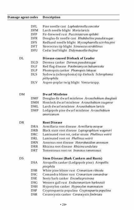
•24•
DFL Pine needle cast Lophodermella concolorDFM Larch needle blight Meria laricisDFP Fir-fireweed rust Pucciniastrum epilobiiDFR Douglas-fir needle cast Rhabdocline pseudotsugaeDFS Redband needle blight Mycosphaerella scirrhia piniDFT Sirococcus tip blight Sirococcus strobilinusDFU Cedar leaf blight Didymascella thujina
DL Disease-caused Dieback of LeaderDLD Dermea canker Dermea pseudotsugaeDLF Red flag disease Potebniamyces balsamicolaDLP Phomopsis canker Phomopsis lokoyaeDLS Sydowia (sclerophoma) tip dieback Sclerophoma
pithyophilaDLV Aspen-poplar twig blight Venturia spp.
DM Dwarf MistletoeDMF Douglas-fir dwarf mistletoe Arceuthobium douglasiiDMH Hemlock dwarf mistletoe Arceuthobium tsugenseDML Larch dwarf mistletoe Arceuthobium laricisDMP Lodgepole pine dwarf mistletoe Arceuthobium
americanum
DR Root DiseaseDRA Armillaria root disease Armillaria ostoyaeDRB Black stain root disease Leptographium wageneriDRC Laminated root rot, cedar strain Phellinus weiriiDRL Laminated root rot Phellinus weiriiDRN Annosus root disease Heterobasidion annosumDRR Rhizina root disease Rhizina undulataDRT Tomentosus root rot Inonotus tomentosus
DS Stem Disease (Bark Cankers and Rusts)DSA Atropellis canker (Lodgepole pine) Atropellis
piniphilaDSB White pine blister rust Cronartium ribicolaDSC Comandra blister rust Cronartium comandraeDSE Sooty bark canker Encoelia pruinosaDSG Western gall rust Endocronartium harknessiiDSH Hypoxylon canker Hypoxylon mammatumDSP Cryptospaeria populina Cryptospaeria populinaDSR Ceratocystis canker Ceratocystis fimbriata
Damage agent codes Description
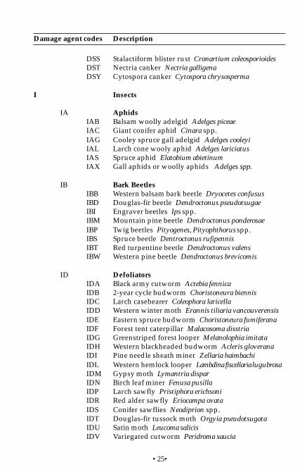
•25•
DSS Stalactiform blister rust Cronartium coleosporioidesDST Nectria canker Nectria galligenaDSY Cytospora canker Cytospora chrysosperma
I Insects
IA AphidsIAB Balsam woolly adelgid Adelges piceaeIAC Giant conifer aphid Cinara spp.IAG Cooley spruce gall adelgid Adelges cooleyiIAL Larch cone wooly aphid Adelges lariciatusIAS Spruce aphid Elatobium abietinumIAX Gall aphids or woolly aphids Adelges spp.
IB Bark BeetlesIBB Western balsam bark beetle Dryocetes confususIBD Douglas-fir beetle Dendroctonus pseudotsugaeIBI Engraver beetles Ips spp.IBM Mountain pine beetle Dendroctonus ponderosaeIBP Twig beetles Pityogenes, Pityophthorus spp.IBS Spruce beetle Dentroctonus rufipennisIBT Red turpentine beetle Dendroctonus valensIBW Western pine beetle Dendroctonus brevicomis
ID DefoliatorsIDA Black army cutworm Actebia fennicaIDB 2-year cycle budworm Choristoneura biennisIDC Larch casebearer Coleophora laricellaIDD Western winter moth Erannis tiliaria vancouverensisIDE Eastern spruce budworm Choristoneura fumiferanaIDF Forest tent caterpillar Malacosoma disstriaIDG Greenstriped forest looper Melanolophia imitataIDH Western blackheaded budworm Acleris gloveranaIDI Pine needle sheath miner Zellaria haimbachiIDL Western hemlock looper Lambdina fiscellaria lugubrosaIDM Gypsy moth Lymantria disparIDN Birch leaf miner Fenusa pusillaIDP Larch sawfly Pristiphora erichsoniIDR Red alder sawfly Eriocampa ovataIDS Conifer sawflies Neodiprion spp.IDT Douglas-fir tussock moth Orgyia pseudotsugataIDU Satin moth Leucoma salicisIDV Variegated cutworm Peridroma saucia
Damage agent codes Description

•26•
IDW Western spruce budworm Choristoneura occidentalisIDX Large aspen tortrix Choristoneura conflictanaIDZ Western false hemlock looper Nepytia freemani
IS Shoot InsectsISB Western cedar borer Trachykele blondeliISE European pine shoot moth Rhyaconia buolianaISG Gouty pitch midge Cecidomyia piniiopisISP Pitch nodule moths Petrova spp.ISQ Sequoia pitch moth Vespamina sequoiaeISS Western pine shoot borer Eucosma sonomana
IW Root and Terminal WeevilsIWC Conifer seedling weevil Steremnius carinatusIWM Magdalis spp.IWP Lodgepole pine terminal weevil Pissodes terminalisIWS White pine weevil (on spruce) Pissodes strobiIWW Warren’s root collar weevil Hylobius warreniIWY Cylindrocopturus weevils Cylindrocopturus spp.IWZ Yosemite bark weevil Pissodes schwartzi
M Mites Trisetacus spp.
N Non-biological Injuries
NB FireND DroughtNF FloodingNG Frost
NGC Frost crackNGH Frost heavedNGK Shoot/bud frost kill
NH HailNK FumekillNL LightningNN Road saltNR RedbeltNS Slide
Damage agent codes Description
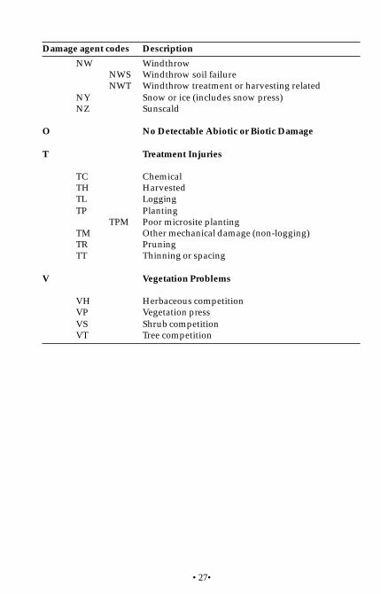
•27•
NW WindthrowNWS Windthrow soil failureNWT Windthrow treatment or harvesting related
NY Snow or ice (includes snow press)NZ Sunscald
O No Detectable Abiotic or Biotic Damage
T Treatment Injuries
TC ChemicalTH HarvestedTL LoggingTP Planting
TPM Poor microsite plantingTM Other mechanical damage (non-logging)TR PruningTT Thinning or spacing
V Vegetation Problems
VH Herbaceous competitionVP Vegetation pressVS Shrub competitionVT Tree competition
Damage agent codes Description
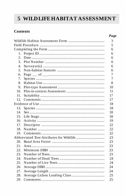
Contents
Wildlife Habitat Assessment Form ......................................... 3Field Procedure .......................................................................... 5Completing the Form ................................................................ 6
1. Project ID .......................................................................... 62. Date ................................................................................... 63. Plot Number .................................................................... 64. Surveyor(s) ...................................................................... 65. Non-habitat features ...................................................... 66. Page ___ of ___ ................................................................ 77. Species .............................................................................. 78. Habitat Use ...................................................................... 89. Plot-type Assessment ..................................................... 10
10. Plot-in-context Assessment ........................................... 1111. Suitability ......................................................................... 1712. Comments ........................................................................ 17
Evidence of Use .......................................................................... 1813. Species .............................................................................. 1814. Sex ..................................................................................... 1815. Life Stage .......................................................................... 1816. Activity ............................................................................. 1917. Descriptor ........................................................................ 2218. Number ............................................................................ 2219. Comments ........................................................................ 22
Abbreviated Tree Attributes for Wildlife ................................ 2320. Basal Area Factor ............................................................ 2321. Area................................................................................... 2322. Minimum DBH ............................................................... 2323. Number of Trees .............................................................. 2324. Number of Dead Trees ................................................... 2425. Number of Live Trees ..................................................... 2426. Average DBH................................................................... 2427. Average Length ............................................................... 2428. Average Lichen Loading Class ..................................... 2529. Comments ........................................................................ 25
5 WILDLIFE HABITAT ASSESSMENT
Page

•2•
Simple Coarse Woody Debris Assessment ............................ 2630. Sampled _ of 30 m Transect ........................................... 2631. Decay Class ...................................................................... 2632. Diameter Class ................................................................ 2833. Comments ........................................................................ 28
Management ............................................................................... 2934. Species .............................................................................. 2935. Use .................................................................................... 2936. Season ............................................................................... 2937. Food/Cover Life Requisite ........................................... 2938. Capability ......................................................................... 2939. Management Techniques ............................................... 3040. Management Feasibility and Intensity ........................ 3041. Comments/Notes ........................................................... 30
Appendix5.1 Wildlife subspecies, species, and species group codes not
included in Cannings and Harcombe (1990) .............. 31
Tables5.1 Codes for types of non-habitat features ............................ 75.2 Codes for distances to nearest non-habitat features ......... 75.3 Specified life requisite codes ............................................. 85.4 Codes for season of use ..................................................... 95.5 Relative quality classes for assessing the plot type
quality relative to the best in B.C. ..................................... 105.6 Habitat features codes for plot-in-context assessment . 115.7 Confidence level codes for assessment of habitat features 155.8 Food/cover life requisite codes ........................................ 155.9 Impact of habitat feature on suitability rating .................. 16
5.10 Codes for life stages for wildlife evidence of use.............. 185.11 Codes for activities and signs of activity .......................... 195.12 Codes for descriptors of wildlife evidence of use ............. 225.13 Decay classes for coarse woody debris ............................. 275.14 Diameter classes for coarse woody debris ........................ 285.15 Codes for management techniques to achieve capability 305.16 Management feasibility/intensity codes for identified
management techniques ................................................... 30Figure 5.1 Top view of biologist standing at center of plot and
estimating the area covering a quarter of the plot andthe number of trees in a quarter plot ........................... 24
Page

•3•
FS
882
(5) H
RE
98/
5
Pro
j. id
.
Plo
t no. 5-
lette
r cod
e
Spe
cies
Sp.
L.R
.S
sn.
FD
SH
TH
Com.
Hab
itat
feat
ure
Conf.
Dis
tanc
e(k
m)
F/C
L.R
.
Com.
Sui
t.Im
p.F
/CL.
R.
FD
SH
TH
Dis
tanc
e(k
m)
Hab
itat
feat
ure
Conf.
Imp.
page
ofN
-hab
.fe
atur
ety
pe
dst.
Sur
veyo
r
Dat
em
yd
Plo
t typ
eH
ab u
se /
Ssn
Plo
t-in
-con
text
Com
men
ts /
Not
es
WILDLIFE HABITAT ASSESSMENT
78
31
9
4
10
25
1211
6

•4•
FS
882
(5) H
RE
98/
5
Pro
ject
id.
Insi
de p
lot
Out
side
plo
t and
insi
de e
cosy
stem
uni
tP
lot n
o.
Evi
denc
e of
Use
Spe
cies
Act
ivity
Sex
Life
Sta
geD
es.
No.
Com
.A
ctiv
ityS
exLi
feS
tage
Des
.N
o.C
om.
No.
Des
.A
ctiv
ityLi
feS
tage
Sex
Abb
revi
ated
Tree
Attr
ibut
es fo
r W
ildlif
e
Com
men
ts /
Not
es
B.A
.F.
No.
of t
rees
Avg
. DB
H (
cm)
Avg
. lic
h lo
ad c
lass
Com
men
ts
No.
dea
d
Are
a
No.
live
Min
DB
H
Avg
. len
gth
(m)
Sim
ple
Coa
rse
Woo
dy D
ebris
Sam
pled
m o
f 30
m tr
anse
ct
Dec
ay c
lass
Dec
ay c
lass
Dia
m. c
lass
Dia
m. c
lass
Com
men
ts
Pie
ce #
Pie
ce #
11
22
33
445 5
6 6
7 7
89
89
10 10
11 11
Man
agem
ent
Spe
cies
(Sp.
gro
up)
Use
Ssn
.F
/C L
R(s
)C
ap.
Mgm
t. Te
ch.
M. F
eat /
Int
Com
men
ts /
Not
es
WILDLIFE HABITAT ASSESSMENT
1918
1716
1514
1918
1716
1514
13
30
3132
33
2225
27
29
2421
2623
28
20
3435
3637
3839
4041

•5•
Field Procedure
Getting Started
1. Determine plot boundaries in consultation with other surveyors.
2. Become familiar with the character of the terrain, soil, and vegetationby traversing the plot and consulting with plant ecologist and soilscientist.
Record and Classify
1. Enter the date, plot number and name(s) of wildlife surveyor(s).
2. Record evidence of use in plot and in ecosystem unit represented bythe plot.
3. List project species and additional species noted during visit.
4. Record habitat use and season for each species.
5. Confer with plant ecologist and soil scientist about site classification,values, and site management concerns.
6. Ensure that relevant wildlife habitat data is filled out on the sitedescription and vegetation forms.
7. Complete coarse woody debris and tree attributes for wildlife forms, ifrequired.
8. Assess the value of the plot-type for each species (not necessary forincidentally recorded species). Be sure that the plot-type assessment iscompleted before the plot-in-context assessment.
9. Assess the value of the plot-in-context for each species based on thespatial context of the plot.
10. Record comments at the bottom of the form, cross-referencing tospecies.
11. Photograph the plot to illustrate important wildlife habitat features orevidence of animal use.
12. Check that all the required information has been collected and notedon the form. Strike through any fields that were not assessed.

•6•
Completing the Form
The purpose of this form is to assess habitat for its value to wildlife and torecord evidence of its usage by wildlife. For inventories of wildlifepopulations, use forms provided in Standardized Inventory Methodologies forComponents of British Columbia’s Biodiversity (Resources Inventory Commit-tee: Elements Working Group 1996) manuals. To record observations ofwildlife outside of the ecosystem unit represented by the plot, use theWildlife Sighting Form available from the B.C. Conservation Data Centre.The Wildlife Sighting Form should be used for observations of all Red andBlue-listed species.
Numbered items below refer to circled numbers on the Wildlife HabitatAssessment Form shown at the beginning of this section. A recommendedsequence for completing the form is described under “Field Procedure.”
1. Project IDIdentify the project as shown on the Site Description form.
2. DateEnter the two-digit codes for year, month, and day.
3. Plot NumberRecord the plot number from the top of the Site Description Form.
4. Surveyor(s)Enter the first initial and last name and of each person involved in complet-ing this form.
5. Non-habitat FeaturesEnter up to two types of human activity or other non-habitat feature (N-hab. feat.) near the plot that may affect usage by wildlife. A non-habitatfeature is a feature of the environment that influences the amount of useof the plot by wildlife. A non-habitat feature can be distinguished froma habitat feature because non-habitat features do not affect habitatattributes (i.e., something measurable to describe habitat) and thereforedo not affect suitability.
Type:Identify the type of prolonged human activity or other non-habitat featurenear the plot using the codes in Table 5.1.

•7•
a This is not a comprehensive list of non-habitat features. For example, disease anddepredation are also examples of non-habitat features that would influence plot-typeusage. Such non-habitat features which are difficult to identify can be noted under thecomments section.
Distance:Enter a code (1–5) indicating the approximate distance (dst.) from theplot to the nearest sites of prolonged human activity or other non-habitatfeatures which may affect wildlife.
TABLE 5.1. Codes for types of non-habitat features a
Code Type
AI Airport (e.g., noise from airplanes and human presence)FA FarmingFE FenceGD Garbage dumpLO Logging activityMI Mining activityOT Other (specify under “Comments”)RF Road traffic, four lanesRO Road traffic, one laneRN Railroad (e.g., noise from trains and human presence)RT Road traffic, two lanesRR Rural (e.g., pressure from human activity)UR Urban/suburban (city, town, village) (e.g., pressure from
human activity)
TABLE 5.2. Codes for distances to nearest non-habitat features
Code Distance
1 0–100 m2 100–250 m3 250–1000 m4 1–5 km5 > 5 km
6. Page ___ of ___If more than one Wildlife Habitat Assessment Form is required for this plot,enter the number of forms used as a total and number each page.
7. SpeciesIndicate the species for which the habitat is being assessed. Use the five-letter codes from Cannings and Harcombe (1990), plus additional codesgiven in Appendix 5.1.

•8•
8. Habitat UseFor each habitat use (Hab use) to be assessed, use one row on the form.
Specified Life Requisite:Specify the life requisite (SpLR) for which the habitat will be used with atwo-letter code from Table 5.3.
TABLE 5.3. Specified life requisite codes
Code Specified life Descriptionrequisite
APa Avoiding pests Habitat used for avoiding pests; e.g., caribouuse snow fields to avoid insects in summer
CO Courting Habitat used for courting; involves enticing aconspecific of the opposite sex into copulation,courtship feeding, and defense of mates
DE Denning/ Habitat used for sleeping or hiding in a cavity,Roosting cave, or burrow; does not include hibernating
nor reproducing-birthing
FS Feeding - Salmon Habitat used for feeding on fish during asalmonid run
HI Hibernating Habitat used for hibernating
LIa Living Habitat used for activities other than;denning, birthing, courting etc.
MDa Migrating daily Habitat used for regular, daily travelling,including travelling away from or towards acommunal habitat; e.g., habitat used by a batfor daily flights to and from a roosting site
MSa Migrating Habitat used for regular, annual travelling; seasonally e.g., habitat used by elk for spring and fall
migrations, or habitat used for travelling awayfrom or towards a communal habitat such as ahibernaculum

•9•
RB Reproducing - Habitat used specifically for giving birth toBirthing live young; e.g., caribou use specialized
habitat for birthing but beaver do not; habitatused by amphibians, birds, and reptiles forhatching of eggs is recorded as habitat usedfor reproduction by eggs (RE)
RE Reproducing - Habitat used for building a nest, laying eggs,Eggs incubation, hatching, and feeding non-mobile
young; reserved for amphibians, birds, andreptiles; specialized habitat used by somemammals to give birth to young is recorded asreproducing-birthing (RB) habitat
SGa Staging Habitat used for staging during spring or fallmigrations
a Activities for which a season needs to be indicated (see below). Theseason is implied for all other activities.
Season:If required, indicate the season (Ssn.) for which the habitat is beingassessed. Use codes listed in Table 5.4. Consult B.C. Wildlife RatingStandards (Resources Inventory Committee: Wildlife InterpretationsSubcommittee 1998) for recommended season coding system for eachspecies.
TABLE 5.4. Codes for season of use
a Early Spring, Late Spring, Early Winter and Late Winter seasons should only be usedfor M-URAR, M-URAM and M-RATA. Also, Early Spring can be used to distinguishEarly Spring feeding habitat from Spring feeding habitat for M-ODVI and M-ODHE.
Code Season Code Season
A All seasons WEa Early WinterG Growing WLa Late WinterW Winter PEa Early SpringP Spring PLa Late SpringS SummerF Fall

•10•
9. Plot-Type AssessmentAssess the food, security habitat and thermal habitat provided by theplot type for the species, use and season being considered. For theseassessments, disregard plot size and shape, and position relative toother habitats. Instead, imagine that the plot type covers a sufficientlylarge area to maximize its value for the species, use and season beingconsidered. This data will be used to establish suitability ratings for theecosystem unit represented by the plot. For assessments of relativequality and suitability use codes in Table 5.5.
For species where it is known that thermal habitat plays a significant role inoverall suitability, but for which thermal qualities of the plot type cannot beassessed separately from the security qualities, do not attempt to enter arating in the TH column—only use the SH column to enter a rating.
TABLE 5.5. Relative quality classes for assessing the plot type quality relative to the best in B.C.
Class Suitability/ Lower limit Upper limit Qualitycapability (%) (%)
1 High > 75 <100 Equivalent2 Mod. high > 50 < 75 Slightly less3 Moderate > 25 < 50 Moderately less4 Low > 5 < 25 Substantially less5 Very low > 0 < 5 Much less6 Nil 0 0 Habitat or attribute
is absent
Food:For species that require food (FD) for the use and season being considered,rate the ability of the plot type to fulfill food requirements.
Security habitat:For species that require security habitat (SH) for the use and season beingconsidered, rate the ability of the plot type to fulfill security requirements.
Thermal habitat:For species that require thermal habitat (TH) for the use and season beingconsidered, rate the ability of the plot type to fulfill thermal requirements.
Comments:To provide additional information about the plot-type assessment, or toclarify an entry made on this line, enter a numeric code (Com.). Enter thesame code in the Comments/Notes section of the form, followed by thepertinent information.
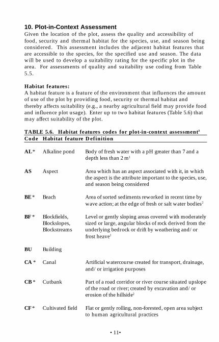
•11•
10. Plot-in-Context AssessmentGiven the location of the plot, assess the quality and accessibility offood, security and thermal habitat for the species, use, and season beingconsidered. This assessment includes the adjacent habitat features thatare accessible to the species, for the specified use and season. The datawill be used to develop a suitability rating for the specific plot in thearea. For assessments of quality and suitability use coding from Table5.5.
Habitat features:A habitat feature is a feature of the environment that influences the amountof use of the plot by providing food, security or thermal habitat andthereby affects suitability (e.g., a nearby agricultural field may provide foodand influence plot usage). Enter up to two habitat features (Table 5.6) thatmay affect suitability of the plot.
TABLE 5.6. Habitat features codes for plot-in-context assessmenta
Code Habitat feature Definition
AL * Alkaline pond Body of fresh water with a pH greater than 7 and adepth less than 2 m1
AS Aspect Area which has an aspect associated with it, in whichthe aspect is the attribute important to the species, use,and season being considered
BE * Beach Area of sorted sediments reworked in recent time bywave action; at the edge of fresh or salt water bodies2
BF * Blockfields, Level or gently sloping areas covered with moderatelyBlockslopes, sized or large, angular blocks of rock derived from theBlockstreams underlying bedrock or drift by weathering and/or
frost heave1
BU Building
CA * Canal Artificial watercourse created for transport, drainage,and/or irrigation purposes
CB * Cutbank Part of a road corridor or river course situated upslopeof the road or river; created by excavation and/orerosion of the hillside2
CF * Cultivated field Flat or gently rolling, non-forested, open area subjectto human agricultural practices
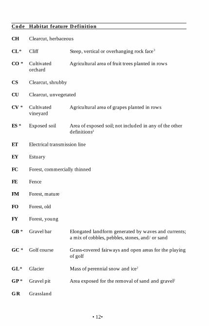
•12•
Code Habitat feature Definition
CH Clearcut, herbaceous
CL * Cliff Steep, vertical or overhanging rock face3
CO * Cultivated Agricultural area of fruit trees planted in rowsorchard
CS Clearcut, shrubby
CU Clearcut, unvegetated
CV * Cultivated Agricultural area of grapes planted in rowsvineyard
ES * Exposed soil Area of exposed soil; not included in any of the otherdefinitions2
ET Electrical transmission line
EY Estuary
FC Forest, commercially thinned
FE Fence
FM Forest, mature
FO Forest, old
FY Forest, young
GB * Gravel bar Elongated landform generated by waves and currents;a mix of cobbles, pebbles, stones, and/or sand
GC * Golf course Grass-covered fairways and open areas for the playingof golf
GL * Glacier Mass of perennial snow and ice2
GP * Gravel pit Area exposed for the removal of sand and gravel2
GR Grassland
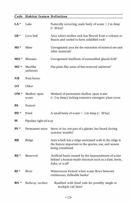
•13•
Code Habitat feature Definition
LA * Lake Naturally occurring, static body of water > 2 m deep(> 50 ha)2
LB * Lava bed Area where molten rock has flowed from a volcano orfissure and cooled to form solidified rock2
MI * Mine Unvegetated area for the extraction of mineral ore andother materials1
MO * Moraine Unvegetated landform of unstratified glacial drift4
MU * Mudflat Flat plain-like areas of fine-textured sediment2
sediment
NB Nest boxes
OT Other
OW * Shallow open Wetland of permanent shallow open waterwater (< 2 m deep); lacking extensive emergent plant cover
PA Pasture
PD * Pond A small body of water > 2 m deep (< 50 ha)
PI Pipeline right-of-way
PS * Permanent snow Snow or ice, not part of a glacier, but found duringsummer months2
RD Ridge Area which has a ridge associated with it; the ridge isthe feature important to the species, use, and seasonbeing considered
RE * Reservoir Artificial basin created by the impoundment of waterbehind a human-made structure such as a dam, berm,dyke, or wall2
RI * River Watercourse formed when water flows betweencontinuous, definable banks2
RN * Railway surface Roadbed with fixed rails for possibly single ormultiple rail lines2
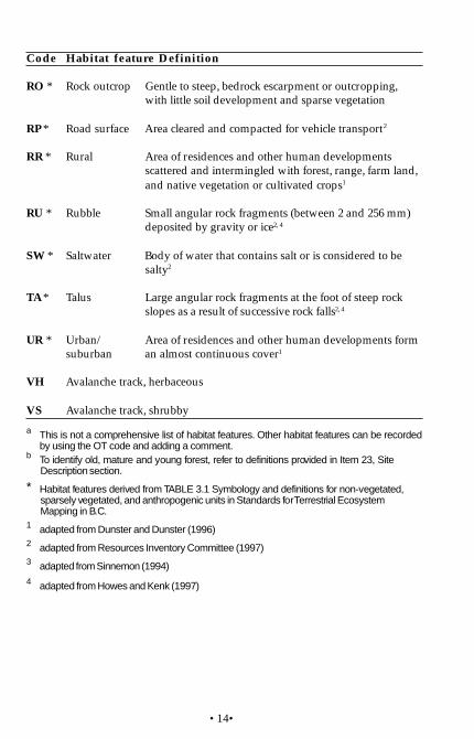
•14•
Code Habitat feature Definition
RO * Rock outcrop Gentle to steep, bedrock escarpment or outcropping,with little soil development and sparse vegetation
RP * Road surface Area cleared and compacted for vehicle transport2
RR * Rural Area of residences and other human developmentsscattered and intermingled with forest, range, farm land,and native vegetation or cultivated crops1
RU * Rubble Small angular rock fragments (between 2 and 256 mm)deposited by gravity or ice2, 4
SW * Saltwater Body of water that contains salt or is considered to besalty2
TA * Talus Large angular rock fragments at the foot of steep rockslopes as a result of successive rock falls2, 4
UR * Urban/ Area of residences and other human developments formsuburban an almost continuous cover1
VH Avalanche track, herbaceous
VS Avalanche track, shrubby
a This is not a comprehensive list of habitat features. Other habitat features can be recordedby using the OT code and adding a comment.
b To identify old, mature and young forest, refer to definitions provided in Item 23, SiteDescription section.
* Habitat features derived from TABLE 3.1 Symbology and definitions for non-vegetated,sparsely vegetated, and anthropogenic units in Standards for Terrestrial EcosystemMapping in B.C.
1 adapted from Dunster and Dunster (1996)2 adapted from Resources Inventory Committee (1997)3 adapted from Sinnemon (1994)4 adapted from Howes and Kenk (1997)
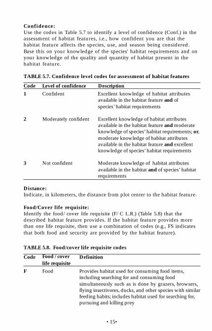
•15•
Confidence:Use the codes in Table 5.7 to identify a level of confidence (Conf.) in theassessment of habitat features, i.e., how confident you are that thehabitat feature affects the species, use, and season being considered.Base this on your knowledge of the species' habitat requirements and onyour knowledge of the quality and quantity of habitat present in thehabitat feature.
TABLE 5.7. Confidence level codes for assessment of habitat features
Code Level of confidence Description
1 Confident Excellent knowledge of habitat attributesavailable in the habitat feature and ofspecies’ habitat requirements
2 Moderately confident Excellent knowledge of habitat attributesavailable in the habitat feature and moderateknowledge of species’ habitat requirements; or,moderate knowledge of habitat attributesavailable in the habitat feature and excellentknowledge of species’ habitat requirements
3 Not confident Moderate knowledge of habitat attributesavailable in the habitat and of species’ habitatrequirements
Distance:Indicate, in kilometers, the distance from plot center to the habitat feature.
Food/Cover life requisite:Identify the food/cover life requisite (F/C L.R.) (Table 5.8) that thedescribed habitat feature provides. If the habitat feature provides morethan one life requisite, then use a combination of codes (e.g., FS indicatesthat both food and security are provided by the habitat feature).
TABLE 5.8. Food/cover life requisite codes
Code Food / cover Definitionlife requisite
F Food Provides habitat used for consuming food items,including searching for and consuming foodsimultaneously such as is done by grazers, browsers,flying insectivores, ducks, and other species with similarfeeding habits; includes habitat used for searching for,pursuing and killing prey

•16•
Code Food / cover Definitionlife requisite
S Security Provides habitat used for protection or hiding frompredators
T Thermal Provides habitat used for protection from heat,cold, or precipitation
Impact:Assess the impact (Imp.) of the habitat feature using codes from Table5.9. Given the presence of the habitat feature, the impact is a measure-ment of the increase or decrease in the quality and accessibility of thefood/cover life requisite(s) relative to quality and accessibility if the plottype extended indefinitely.
TABLE 5.9. Impact of habitat feature on suitability rating
Code Description
1 Large increase2 Moderate increase3 Low increase4 No effect5 Low decrease6 Moderate decrease7 Large decrease
Food:Considering the context of the plot, for species that require food (FD) forthe use and season being considered, rate the overall quality andaccessibility of food. Use coding from Table 5.5.
Security habitat:Considering the context of the plot, for species that require securityhabitat (SH) for the use and season being considered, rate the overallquality and accessibility of security habitat. Use coding from Table 5.5.
Thermal habitat:Considering the context of the plot, for species that require thermalhabitat (TH) for the use and season being considered, rate the overallquality and accessibility of thermal habitat. Use coding from Table 5.5.

•17•
11. SuitabilityAssign a suitability rating (Suit.), using the codes in Table 5.5, for theplot-in-context, for the species, use, and season being considered. Basethe suitability on the ratings entered in the food (FD), security habitat(SH), and thermal habitat (TH) columns. Theoretically, the suitabilityrating should be an average or weighted average of the three food/coverlife requisite ratings.
12. CommentsTo provide additional information about the habitat assessment, or toclarify an entry on this line on the form, enter a numeric code (Com). Enterthe same code in the Comments/Notes section of the form, followed by thepertinent information.

•18•
Evidence of Use
Complete this section if there is any evidence of use by wildlife. Evidenceof use can be in the plot boundaries or in the ecosystem unit represented bythe plot.
13. SpeciesIndicate the species for which the evidence of use is being recorded. Usethe five-letter codes from Cannings and Harcombe (1990), plus additionalcodes given in Appendix 5.1.
14. SexNote the sex of the animal. Code as M (male), F (female), or U (unknown).
15. Life StageRecord the life stage of the animal using the codes in Table 5.10. Notethat these classes differ from those described in the StandardizedInventory Methodologies for Components of B.C.’s Biodiversity (ResourcesInventory Committee: Elements Working Group 1996).
TABLE 5.10. Codes for life stages for wildlife evidence of use
Code Life stage Description
E Egg Amphibian, bird, insect, and reptile eggs
N Nestling Nestling birds and newly hatched or newbornor neonate newborn amphibians, birds, insects, mammals, and
reptiles; only used when it is apparent that the nestsite is within the plot type
J Juvenile Amphibian larvae, fledged birds before their firstwinter, insect larvae, and mammals older thanneonates, but still requiring parental care; reptilesdo not have a juvenile stage
S Subadult Animal that is older than the juvenile stage, doesnot require parental care, and has not reachedsexual maturity; includes amphibians and reptileswhich have not reached adult size, but have adultform; insects have no subadult stage
A Adult Old enough to breed
U Undetermined Life stage is unknown
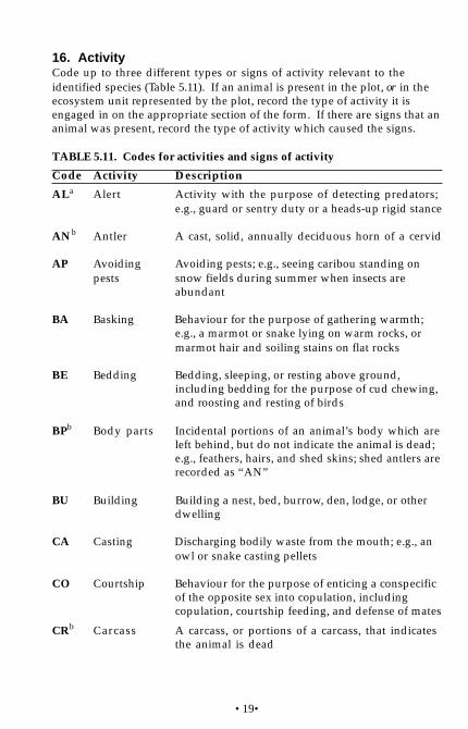
•19•
16. ActivityCode up to three different types or signs of activity relevant to theidentified species (Table 5.11). If an animal is present in the plot, or in theecosystem unit represented by the plot, record the type of activity it isengaged in on the appropriate section of the form. If there are signs that ananimal was present, record the type of activity which caused the signs.
TABLE 5.11. Codes for activities and signs of activity
Code Activity Description
ALa Alert Activity with the purpose of detecting predators;e.g., guard or sentry duty or a heads-up rigid stance
ANb Antler A cast, solid, annually deciduous horn of a cervid
AP Avoiding Avoiding pests; e.g., seeing caribou standing onpests snow fields during summer when insects are
abundant
BA Basking Behaviour for the purpose of gathering warmth;e.g., a marmot or snake lying on warm rocks, ormarmot hair and soiling stains on flat rocks
BE Bedding Bedding, sleeping, or resting above ground,including bedding for the purpose of cud chewing,and roosting and resting of birds
BPb Body parts Incidental portions of an animal’s body which areleft behind, but do not indicate the animal is dead;e.g., feathers, hairs, and shed skins; shed antlers arerecorded as “AN”
BU Building Building a nest, bed, burrow, den, lodge, or otherdwelling
CA Casting Discharging bodily waste from the mouth; e.g., anowl or snake casting pellets
CO Courtship Behaviour for the purpose of enticing a conspecificof the opposite sex into copulation, includingcopulation, courtship feeding, and defense of mates
CRb Carcass A carcass, or portions of a carcass, that indicatesthe animal is dead
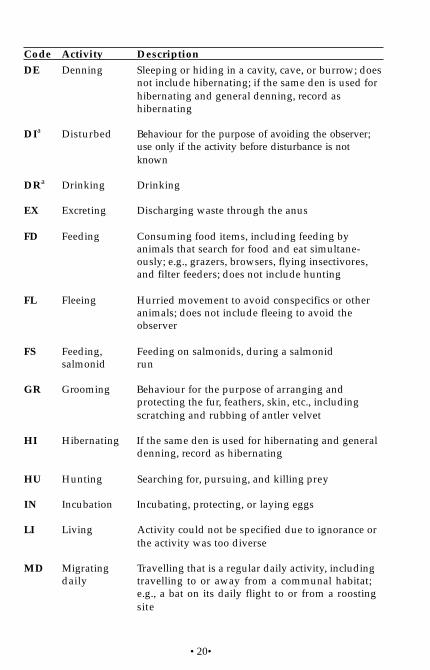
•20•
Code Activity Description
DE Denning Sleeping or hiding in a cavity, cave, or burrow; doesnot include hibernating; if the same den is used forhibernating and general denning, record ashibernating
DIa Disturbed Behaviour for the purpose of avoiding the observer;use only if the activity before disturbance is notknown
DRa Drinking Drinking
EX Excreting Discharging waste through the anus
FD Feeding Consuming food items, including feeding byanimals that search for food and eat simultane-ously; e.g., grazers, browsers, flying insectivores,and filter feeders; does not include hunting
FL Fleeing Hurried movement to avoid conspecifics or otheranimals; does not include fleeing to avoid theobserver
FS Feeding, Feeding on salmonids, during a salmonidsalmonid run
GR Grooming Behaviour for the purpose of arranging andprotecting the fur, feathers, skin, etc., includingscratching and rubbing of antler velvet
HI Hibernating If the same den is used for hibernating and generaldenning, record as hibernating
HU Hunting Searching for, pursuing, and killing prey
IN Incubation Incubating, protecting, or laying eggs
LI Living Activity could not be specified due to ignorance orthe activity was too diverse
MD Migrating Travelling that is a regular daily activity, includingdaily travelling to or away from a communal habitat;
e.g., a bat on its daily flight to or from a roostingsite

•21•
Code Activity Description
MS Migrating Travelling that is a regular annual activity;seasonally e.g., an elk or a Sandhill Crane on its migration
route, or a snake travelling away from a communalhabitat such as a hibernaculum
RB Reproducing, Giving birth to live young; preparing a birthingbirthing reproduction site, such as a den
RE Reproducing, Laying eggs (amphibians, reptiles and birds),eggs building a nest, and feeding non-mobile young
RR Rearing Adults feeding neonates and juveniles
SH Security Using habitat for protection or hiding fromhabitat predators
ST Security and/ Using habitat for its security and/or thermalor thermal values; used when differentiating between the two
values is difficult or impossible
TE Territoriality Behavior for the purpose of marking or defending aterritory; e.g., singing, drumming, winnowing,howling, antler rubbing, wallowing, or scraping theground
TFa Travelling, Used when the purpose of flying is not known;flying if known, use a more specific description such as
hunting
TH Thermal Using habitat for protection from heat, cold, orhabitat precipitation
TP Travelling Walking on a trail that is embedded in theon a path ground due to animals walking the same route for
many years
TR Travelling Travelling by a method other than flying, swim-ming, and walking; usually used for animals thatdo not normally fly, swim, or walk; includes seeingan isolated track; does not include running if thepurpose for running is known

•22•
Code Activity Description
TSa Travelling, Used when the specific purpose of swim-swimming ming is not known; if known, use a more specific
description such as fleeing
TW Travelling, Used when the purpose of walking is notwalking known; if known, use a more specific description
such as migrating; does not include travelling on apath (see “TP”)
UR Urinating Urinatinga Code is only associated with seeing or hearing an animalb Code is only associated with sign of an animal
17. DescriptorEnter a coded descriptor (Des) that indicates whether the animal wasobserved or heard in the plot or ecosystem unit, or gives the probable ageor season of the sign (Table 5.12).
TABLE 5.12. Codes for descriptors of wildlife evidence of use
Code Meaning
S The animal was seenH The animal was heardF Fresh sign (<1 week old)Y Sign is <1 year old but >1 week oldO Old (>1 year old)U Undetermined (age of sign is unknown)W Sign is from the winter seasonG Sign is from the growing season
18. NumberRecord the number (No.) of animals present or the number of sign ele-ments. Codes for relative abundance can be used for sign elements insteadof numbers (i.e., H [high], M [moderate], L [low], or T [trace]).
19. CommentsTo provide additional information about the evidence of use, or to clarifyan entry on this line on the form, enter a numeric code (Com). Enter thesame code in the Comments/Notes section of the form, followed by thepertinent information.

•23•
For a variable radius plot do a prism sweep while counting thenumber of trees in the plot.
For a fixed area plot stand at the plot center and while holdingarms out at right angles to each other (Figure 5.1) estimate thearea and number of trees in one quarter of the plot. Then turn 90degrees and while holding arms out, repeat the estimate for thesecond quarter. Do this for all four quarters. Total the values toobtain the number of trees.
• Complete the Abbreviated Tree Attributes for Wildlife portion of theform based upon the trees selected in the step above.
20. Basal Area FactorIf a variable radius plot is used, enter the standard metric Basal Area Factor(BAF) in m2/ha.
21. AreaIf a fixed area plot is used, enter the area of the plot, in m2.
22. Minimum DBHEnter the minimum diameter at breast height (Min DBH) being used (in cm).
23. Number of TreesRecord the number of trees (No. of trees) in the variable radius or fixedarea plot.
Abbreviated Tree Attributes for Wildlife
The purpose of this section of the form is to provide for a quick assessmentof selected tree attributes for wildlife. The data recorded here is abbreviatedand more qualitative than that collected using the detailed Tree Attributesfor Wildlife Form (Section 6). Refer to Section 6 for information on selectingthe sampling method. Once selected, the same sampling method should beused consistently throughout the project.
Also, refer to Section 6 for information on selecting the prism BAF or plotsize, and minimum DBH. Once the prism or plot size is determined for theplot, complete appropriate sections of the Wildlife Habitat AssessmentForm.
Field Procedures
• Establish plot center
• Stand at the plot center and estimate the number of trees in the plotasfollows:
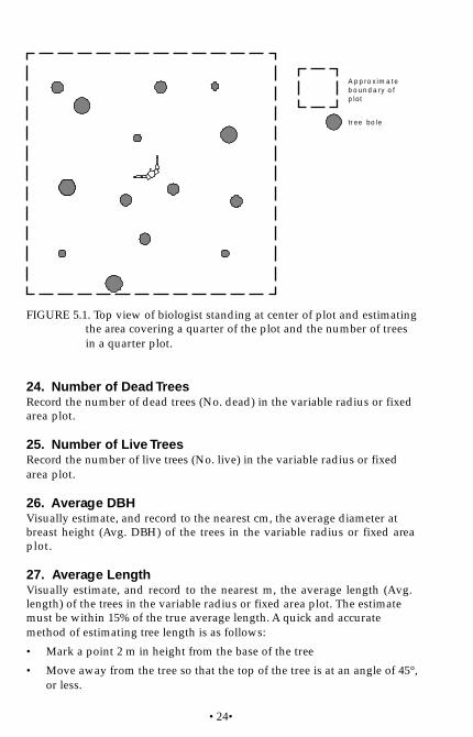
•24•
FIGURE 5.1. Top view of biologist standing at center of plot and estimating the area covering a quarter of the plot and the number of trees in a quarter plot.
tr ee bo le
A p p ro x im a t eb o un d a ry o fp lo t
24. Number of Dead TreesRecord the number of dead trees (No. dead) in the variable radius or fixedarea plot.
25. Number of Live TreesRecord the number of live trees (No. live) in the variable radius or fixedarea plot.
26. Average DBHVisually estimate, and record to the nearest cm, the average diameter atbreast height (Avg. DBH) of the trees in the variable radius or fixed areaplot.
27. Average LengthVisually estimate, and record to the nearest m, the average length (Avg.length) of the trees in the variable radius or fixed area plot. The estimatemust be within 15% of the true average length. A quick and accuratemethod of estimating tree length is as follows:
• Mark a point 2 m in height from the base of the tree
• Move away from the tree so that the top of the tree is at an angle of 45°,or less.
•25•
• Tilt your head so that by rolling your eyes, and not moving your head,you can see the bottom and top of the tree.
• Hold a piece of twig or grass vertically between your thumb and indexfinger, and about 20 cm from your face. Adjust the length of the twig sothat it spans the 2 m distance marked at the bottom of the tree.
• Move the twig upward vertically, and while rolling your eyes, count thenumber of twig-lengths that fit between the bottom of the tree and thetop. When moving the twig upward it is important to keep the twigvertical and in the same plane, and your head still.
• Multiply the number of twig-lengths by two to obtain the length of thetree, in metres.
28. Average Lichen Loading ClassVisually estimate and record the average lichen loading class (Avg. lichload class) of the wildlife trees in the plot. Assign a rating (0–5) based oncomparison with photos in Estimating the Abundance of Arboreal ForageLichens (Armleder et al. 1992).
29. CommentsRecord observations on tree attributes deemed to be of importance towildlife.
•26•
Simple Coarse Woody Debris Assessment
The purpose of this section of the form is to provide for a quick assessmentof total coarse woody debris volume and volume by decay classes follow-ing the methods developed by Taylor (1997). The detailed Coarse WoodyDebris Form (Section 7) is used both to collect more quantitative data thanthat collected here and to collect more attributes.
To complete this section of the form, set up a 30 m line transect as follows:
1. Determine plot centre
2. Establish one 30 m (horizontal distance) line transect following arandom azimuth from the plot centre. It is important to measure theslope along the line and determine the slope distance required toproduce a horizontal transect of 30 m. If significant slope changes occuralong the line, more than one slope distance correction is required.
3. The slope distance factors in Table 4.1 can be used to calculate therequired slope distance for a given slope. For example, if the slope is35%, the slope distance factor is 0.944. The required slope distance isdetermined by dividing the horizontal distance by the slope distancefactor, i.e., 30 m / 0.944 = 31.78 m.
30. Sampled __ of 30 m TransectIndicate the length of the line that was sampled. The form has room torecord 22 pieces of CWD. If more than 22 pieces are encountered on a 30 mtransect, discontinue the transect and record the number of metres thatwere sampled to reach 22 pieces. If the entire line was sampled, indicatethat all 30 m were sampled.
31. Decay ClassAssign a decay class (1 to 5) based on the majority condition of eachpiece encountered along the transect. See Table 5.13 for descriptions ofclasses.
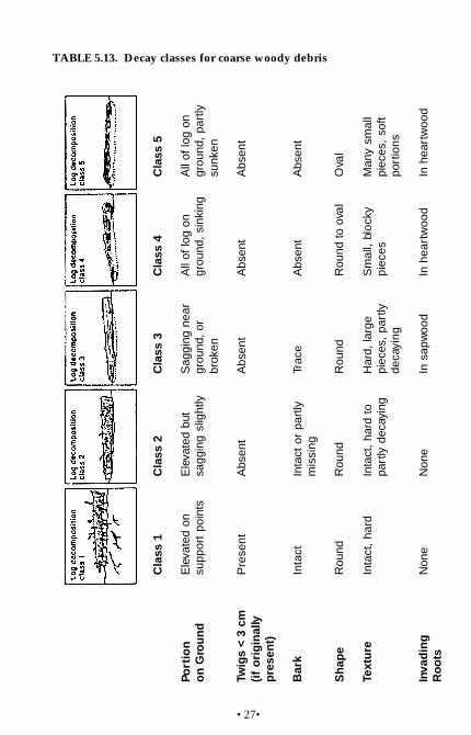
•27•
Port
ion
on G
roun
d
Twig
s <
3 cm
(if o
rigin
ally
pres
ent)
Bar
k
Sha
pe
Text
ure
Inva
ding
Roo
ts
Cla
ss 1
Ele
vate
d on
supp
ort
poin
ts
Pre
sent
Inta
ct
Rou
nd
Inta
ct,
hard
Non
e
Cla
ss 2
Ele
vate
d bu
tsa
ggin
g sl
ight
ly
Abs
ent
Inta
ct o
r pa
rtly
mis
sing
Rou
nd
Inta
ct,
hard
to
part
ly d
ecay
ing
Non
e
Cla
ss 3
Sag
ging
nea
rgr
ound
, or
brok
en
Abs
ent
Trac
e
Rou
nd
Har
d, la
rge
piec
es,
part
lyde
cayi
ng
In s
apw
ood
Cla
ss 4
All
of lo
g on
grou
nd,
sink
ing
Abs
ent
Abs
ent
Rou
nd to
ova
l
Sm
all,
bloc
kypi
eces
In h
eart
woo
d
Cla
ss 5
All
of lo
g on
grou
nd,
part
lysu
nken
Abs
ent
Abs
ent
Ova
l
Man
y sm
all
piec
es,
soft
port
ions
In h
eart
woo
d
TABLE 5.13. Decay classes for coarse woody debris
•28•
32. Diameter ClassUsing the diameter class limits from Table 5.14, record the diameterclass (Diam. class) at the point of intersection for each piece encounteredalong the transect.
TABLE 5.14. Diameter classes for coarse woody debris
33. CommentsRecord observations of interest or importance to making wildlife interpreta-tions.
Class Range (cm)
10 > 7.5 – 12.515 12.6 – 17.520 17.6 – 22.525 22.6 – 27.530 27.6 – 32.535 32.6 – 37.540 37.6 – 42.545 42.6 – 47.550 47.6 – 52.555 52.6 – 57.560 57.6 – 62.565 62.6 – 67.570 67.6 – 72.5
Code Range (cm)
75 72.6 – 77.5 80 77.6 – 82.5 85 82.6 – 87.5 90 87.6 – 92.5 95 92.6 – 97.5100 97.6 – 102.5105 102.6 – 107.5110 107.6 – 112.5115 112.6 – 117.5120 117.6 – 122.5125 122.6 – 127.5130 127.6 – 132.5135 132.6 – 137.5

•29•
Management
This section is to be completed for species or species groups, according tothe project objectives, for which specific management prescriptions may beimplemented.
If the suitability of a habitat for a particular species (as evaluated in Item11) is lower than its capability, it may be possible to apply habitat manage-ment techniques to achieve the capability of the habitat. Table 5.15 listsmanagement practices of a low technological order, e.g., prescribedburning, livestock control, prescribed logging, that may be possible toprescribe in order to modify certain habitat conditions.
The approach is as follows: considering adjacent habitat features and thecurrent value of the plot for a specific species, use, and season, how couldthe ecosystem unit represented by the plot be managed to optimize thesuitability of the area?
34. SpeciesFrom the list of species evaluated on the plot, indicate the species for whichthe habitat could be managed. Use the five-letter codes as in Item 7.
35. UseWith a two-letter code from Table 5.3, indicate the specified life requisite forwhich the habitat will be managed. Use additional rows on the form toassess the habitat for more than one habitat use.
36. SeasonIf required, indicate the season (Ssn) for which the habitat will be managed.Use codes listed in Table 5.4.
37. Food/Cover Life RequisiteIdentify the food/cover life requisite (F/C LR), using the codes in Table 5.8,that will be most affected by the management technique described below. Ifthe management technique affects more than one life requisite, then use acombination of codes (e.g., FS indicates that both food and security areaffected).
38. CapabilityConsidering the presence of habitat features, rate the capability (Cap) of theplot to meet the specified use in the specified season for the selected speciesor species group. Use the codes in Table 5.5. Capability is the ability of thehabitat under optimal conditions to provide life requisites for the species.

•30•
It is assumed that the management techniques identified below will resultin the habitat attaining these optimal conditions.
39. Management TechniquesIdentify the management technique(s) (Mgmt. Tech.) from the list inTable 5.15 that would result in the assigned capability.
TABLE 5.15. Codes for management techniques to achieve capability
Code Management technique
PF Prescribed fireMT Mechanical treatment (slashing/brushing)PL Seeding & plantingTS Thinning & spacingSC Selective cuttingCC ClearcuttingPR Protection (to maintain current conditions)GR Prescribed grazingNG No grazingWL Water level manipulationNC Nest constructionOT Other
40. Management Feasibility and IntensityIndicate the feasibility of management or the management intensity(M. Fea/Int) required to fulfill the objectives. Use the codes in Table 5.16.
TABLE 5.16. Management feasibility/intensity codes for identified management techniques
Code Feasibility/intensity
NR Not required; habitat is in optimum conditionIM Impractical; desired changes would take too longNA Not appropriate; management would affect the ecosystemCM Constant management required (every 2-5 years)FM Frequent management required (every 5-10 years)MM Moderate management required (every 10-20 years)IF Infrequent management required (every 20-50 years)
41. Comments/NotesRecord comments that may assist in developing management prescriptions.

•31•
APPENDIX 5.1Wildlife subspecies, species and speciesgroup codes not included in Canningsand Harcombe (1990).
Subspecies codes are derived from the species code; the last letter of thespecies code is replaced with the first letter of the Latin subspecies name.Species Groups begin the four-letter group code with the letter "U" followedby three letters derived from the common name of the species group. (e.g.,unspecified grouse = BUGRU.) Species names preceded by an asterix are inCannings and Harcombe (1990), and are included here for convenience.
AMPHIBIANS AND REPTILES
Salamanders Order CaudataUnspecified Salamander (unspecified) A-USAL
Frogs and Toads Order AnuraUnspecified Frog (unspecified) A-UFRO
Turtles Order TestudinesUnspecified Turtle (unspecified) R-UTUR
Lizards Order SquamataUnspecified Lizard (unspecified) R-ULIZ
Snakes Order SerpentesUnspecified Snake (unspecified) R-USNA
MAMMALS
Insectivores Order InsectivoraUnspecified Mole (unspecified) M-UMOLUnspecified Shrew (unspecified) M-USHR
Bats Order ChiropteraUnspecified Bat (unspecified) M-UBAT
Rodents Order RodentiaUnspecified Chipmunk (unspecified) M-UCHPUnspecified Jumping Mouse (unspecified) M-UJUMUnspecified Mouse (unspecified) M-UMOUUnspecified Vole (unspecified) M-UVOL

•32•
Carnivores Order CarnivoraBlack Bear Ursus americanus M-URAMCougar* Felis concolor M-FECODomestic Cat Felis sylvestris M-FESYDomestic Dog Canis familiarius M-CAFAFisher* Martes pennanti M-MAPEGray Wolf* Canis lupus M-CALUGrizzly Bear* Ursus arctos M-URARMarten* Martes americana M-MAAMUnspecified Bear (unspecified) M-UBEAUnspecified Sea Lion (unspecified) M-USELUnspecified Weasel (unspecified) M-UWEA
Ungulates Order ArtiodactylaAlaska Moose Alces alces gigas M-ALAGBighorn Sheep* Ovis canadensis M-OVCABlack-tailed Deer Odocoileus hemionus columbianus M-ODHCCalifornia Bighorn Sheep Ovis canadensis californiana M-OVCCDall Sheep Ovis dalli dalli M-OVDDElk* Cervus elaphus M-CEELInterior Mule Deer Odocoileus hemionus hemionus M-ODHHMoose* Alces alces M-ALALMule Deer* Odocoileus hemionus M-ODHENorthwestern Moose Alces alces andersoni M-ALAARocky Mountain Bighorn Sheep Ovis canadensis canadensis M-OVCNRocky Mountain Elk Cervus elaphus nelsoni M-CEENRoosevelt Elk Cervus elaphus roosevelti M-CEERSitka Deer Odocoileus hemionus sitkensis M-ODHSStone Sheep Ovis dalli stonei M-OVDSThinhorn Sheep* Ovis dalli M-OVDAWhite-tailed Deer* Odocoileus virginiana M-ODVIYellowstone Moose Alces alces shirasi M-ALASDomestic Cow Bos taurus M-BOTADomestic Goat Capra hircus M-CAHIDomestic Horse Equus caballus M-EQCADomestic Pig Sus scrofa M-SUSCUnspecified Deer (unspecified) M-UDEE
Whales and Porpoises Order CetaceaUnspecified Dolphin (unspecified) M-UDOLUnspecified Whale (unspecified) M-UWHA

•33•
BIRDS
Loons Order GaviiformesUnspecified Loon (unspecified) B-ULOO
Grebes Order PodicipediformesUnspecified Grebe (unspecified) B-UGRE
Albatrosses, Shearwaters Order Procellariiformesand PetrelsUnspecified Albatross (unspecified) B-UALBUnspecified Shearwater (unspecified) B-USHEUnspecified Storm-Petrel (unspecified) B-USTP
Pelicans and Cormorants Order PelecaniformesUnspecified Cormorant (unspecified) B-UCOR
Waterfowl Order AnseriformesDomestic/feral duck (Peking) Anas platyrhynchos B-DODUDomestic/feral goose (Greylag) Anser answer B-DOGSMuskovy Duck Cairina maschata B-MUDUUnspecified Dabbling Duck (unspecified) B-UDADUnspecified Diving Duck (unspecified) B-UDIDUnspecified Goldeneye (unspecified) B-UGOLUnspecified Merganser (unspecified) B-UMERUnspecified Scaup (unspecified) B-USCAUnspecified Scoter (unspecified) B-USCOUnspecified Swan (unspecified) B-USWNUnspecified Teal (unspecified) B-UTEA
Vultures, Hawks, and Falcons Order FalconiformesUnspecified Eagle (unspecified) B-UEAGUnspecified Falcon (unspecified) B-UFALUnspecified Hawk (unspecified) B-UHAW
Gallinaceous Birds Order GalliformesUnspecified Grouse (unspecified) B-UGRUUnspecified Ptarmigan (unspecified) B-UPTA
Shorebirds, Gulls, Auks, Order Charadriiformesand AlliesUnspecified Auklet (unspecified) B-UAUKUnspecified Gull (unspecified) B-UGULUnspecified Murre (unspecified) B-UMURUnspecified Murrelet (unspecified) B-UMULUnspecified Puffin (unspecified) B-UPUFUnspecified Shorebird (unspecified) B-USHO
Pigeons and Doves Order ColumbiformesUnspecified Dove (unspecified) B-UDOV

•34•
Owls Order StrigiformesUnspecified Owl (unspecified) B-UOWL
Swifts and Hummingbirds Order CaprimulgiformesUnspecified Hummingbird (unspecified) B-UHUMUnspecified Swift (unspecified) B-USWI
Woodpeckers Order PiciformesUnspecified Woodpecker (unspecified) B-UWOO
Passerine Birds Order PasseriformesUnspecified Blackbird (unspecified) B-UBLAUnspecified Bluebird (unspecified) B-UBLUUnspecified Chickadee (unspecified) B-UCHIUnspecified Crossbill (unspecified) B-UCROUnspecified Finch (unspecified) B-UFINUnspecified Flycatcher (unspecified) B-UFLYUnspecified Grosbeak (unspecified) B-UGROUnspecified Kinglet (unspecified) B-UKINUnspecified Longspur (unspecified) B-ULONUnspecified Nuthatch (unspecified) B-UNUTUnspecified Redpoll (unspecified) B-UREDUnspecified Shrike (unspecified) B-USHIUnspecified Sparrow (unspecified) B-USPAUnspecified Swallow (unspecified) B-USWAUnspecified Thrush (unspecified) B-UTHRUnspecified Vireo (unspecified) B-UVIRUnspecified Warbler (unspecified) B-UWARUnspecified Waxwing (unspecified) B-UWAXUnspecified Wren (unspecified) B-UWRE

•35•
Contents
Tree Attributes for Wildlife Form ............................................ 3Field Procedure .......................................................................... 4Selecting the Sampling Method .............................................. 5Selecting the Minimum Diameter .......................................... 5Selecting a Basal Area Factor Prism ....................................... 5Selecting the Plot Size and Shape ........................................... 5Completing the Form ............................................................... 6
1. Project Identification ...................................................... 62. Date ................................................................................... 63. Surveyor ........................................................................... 64. Plot Number .................................................................... 65. Basal Area Factor ............................................................ 66. Plot Size ............................................................................ 67. Minimum Diameter ....................................................... 68. Species .............................................................................. 69. Standing/Fallen .............................................................. 6
10. Diameter at Breast Height ............................................. 711. Measured or Estimated ................................................. 712. Remaining Bark .............................................................. 713. Length .............................................................................. 7
Slope to top of tree ...................................................... 7Slope to DBH or bottom of tree ................................ 8Bottom position ........................................................... 8Slope distance .............................................................. 8
14. Estimated Length ........................................................... 815. Crown Class .................................................................... 816. Height to Live Crown .................................................... 817. Wildlife Codes ................................................................. 9
Appearance .................................................................. 9Crown condition ......................................................... 9Bark retention ............................................................... 9Wood condition ........................................................... 10Lichen loading ............................................................. 10Wildlife use ................................................................... 10
6 TREE ATTRIBUTES FOR WILDLIFE
Page
•2•
Appendix6.1 Tree species codes ........................................................... 13
Tables6.1 Crown condition codes ................................................. 96.2 Bark retention codes ...................................................... 106.3 Wood retention codes .................................................... 10
Figures6.1 Visual appearance codes for wildlife trees ................ 9
Page

•3•
FS
882
(6) H
RE
98/
5
CrownBark
Wood
Lichen
Wildlifeuse
Cr. Class
Bo
tpo
s(m
)
Leng
thC
om
me
nts
Estimatedlength (m)
M or E
DB
H (c
m)
Tree
No.
10 0 0 0
2 3 4
05
06
07
08
09
10
11
12
13
14
15
16
17
18
19
20
Spe
cies
Pro
ject
id.
Plo
t no.
Sur
veyo
r
B.A
.F (
m2 /
ha)
Stand/FallR
em.
Bark
(%)
Plo
t siz
e (m
2 )M
inim
um D
BH
(cm
)
Top
(%)
Bo
t(%
)S
lope
Dis
tanc
e(m
)
Hei
ght
to live
crow
n(m
)
Appear
Wild
life
Cod
es
Dat
ey
md
TREE ATTRIBUTES FOR WILDLIFE
1
5
3
89
1011
1213
6
1415
16
4
1772

•4•
Field Procedure
Getting Started
1. Identify sample trees based on a prism sweep, or if using a fixed-areaplot, establish plot boundaries. Be aware of the minimum DBH for theproject.
2. If desired, tag or flag numbers on each tree including all live and dead,standing and fallen trees.
Measure and Record
1. Enter the header information.
2. For each sample tree, record the species and classify as standing orfallen.
3. Determine DBH and percentage of bark remaining at breast height.
4. Record data required to calculate the length of each sample tree, orestimate length.
5. For each standing live tree, assign a crown class and determine height tolive crown.
6. For each sample tree, assess appearance, crown condition, bark reten-tion, wood condition, lichen loading, and wildlife use.
7. Check that all the required information has been collected and noted onthe form. Strike through any fields that were not assessed.

•5•
Selecting the Sampling Method
Either a fixed-area or variable-radius plot may be used. Variable-radius plotswill be used most commonly, but if the project area is dominated by standswith the following characteristics, a fixed-area plot may be preferable:
• very open stands with widely spaced trees or clumps of trees
• very dense stands where not all trees in a plot would be easily visible
Once selected, the same plot-type should be used consistently throughoutthe project.
Selecting the Minimum DiameterThe minimum diameter at breast height (DBH) is determined by the wildlifespecies of concern in the project—the goal is to sample a reasonable numberof trees of an appropriate minimum size for the species. For example, forBald Eagle interpretations, trees less than 20 cm DBH are not of value andmay be ignored. For most projects, the minimum DBH will be 15 cm orgreater. Trees less than the minimum DBH are ignored
Selecting a Basal Area Factor PrismThe basal area factor (BAF) prism size should be based on previous experi-ence. A prism size that will provide 7-11 sample trees (greater than or equalto the minimum DBH) per plot is ideal. A minimum of 5 and maximum of 16trees is required. Generally, the larger the trees, the larger the BAF; thedenser the stand, the smaller the BAF required. It may be necessary to haveseveral prisms available throughout a project. When traversing the stand,but before determining the plot location, the prism size should be selected.
Selecting the Plot Size and ShapeFor fixed-area plot sampling, a plot size is selected that will provide ten ormore sample trees greater than or equal to the minimum DBH. The plot sizeis determined for a project and is only reduced or increased in exceptionalcircumstances. The decision of whether to increase or decease, e.g., double orhalve, the plot size is done when entering the stand, before the plot ismarked, so as to minimize bias.
Plot shape can be circular, square, or rectangular, but should be determinedat the start of a project.
•6•
Completing the Form
Numbered items below refer to circled numbers on the Tree Attributes forWildlife Form shown at the beginning of this section. A recommendedsequence for completing the form is described under “Field Procedure.”
1. Project IdentificationIdentify the project (Proj id.) as in Item 3, Site Description Form.
2. DateEnter the 2-digit codes for year, month, and day.
3. SurveyorEnter the first initial and last name of person(s) collecting tree attribute data.
4. Plot no.Record the plot number from the Site Description Form.
5. Basal Area FactorEnter the standard metric (m2/ha) Basal Area Factor (BAF) prism used, ifapplicable.
6. Plot sizeEnter the area of the plot, if applicable.
7. Minimum DiameterEnter the minimum diameter (DBH) being used.
8. SpeciesIdentify tree species using the codes given in Appendix 6.1.
9. Standing / FallenClassify the tree as standing or fallen using the following codes and criteria:
S Standing Trees or portions of trees with the root attached and self-supporting (i.e., the tree would remain standing if all supportingmaterials were removed).
F Fallen Trees or portions of trees with the root attached and not self-supporting, greater than 1.3 m in length.

•7•
10. Diameter at Breast HeightMeasure the diameter at breast height (DBH), i.e., 1.3 m, of all live, dead,standing, and fallen sample trees.
• On slopes, breast height is measured from the high side of the tree.
• Measure diameter to the nearest 0.1 cm.
• Hold the diameter tape tight, making no allowance for missing bark.
• If it is not possible to measure DBH accurately because of an obstructionor unsafe conditions, enter an estimate.
11. Measured or EstimatedIf it was necessary to estimate DBH, enter E; otherwise, enter M.
12. Remaining BarkRecord, to the nearest percent, the percentage of bark remaining at breastheight. Use the diameter tape to measure the total circumference and theportion of the circumference with bark remaining. The ratio of the twonumbers multiplied by 100 equals the percent remaining bark. For example,if a tree with a 60 cm circumference has bark remaining on 15 cm, thepercent remaining is 15 ÷ 60 × 100 = 25%. Note the following codingconvention:
• Record 100% bark remaining as “– –”. When the data is entered into adatabase, e.g., VENUS, substitute 100 for “– –”.
• If no bark is present, record as “00”.
13. LengthDetermine the total length of all trees greater than 1.3 m high by collectingall the information required to complete the fields on the form. Measurelength from the ground surface on the high side of the stem, along the stem,to the top.
• If the tree is broken, record the length of the stem to the point of break-age.
• On fallen trees, measure from the root collar to the top of the lastattached portion of the stem.
• Length may be estimated if it is not possible to measure accuratelybecause of obstructions, unsafe conditions, or if project objectives do notrequire measured accuracy on all trees.
Slope to top of tree (Top):Enter the percent slope to the top of the tree; the sign must be shown(usually ‘+’). The maximum acceptable reading is 99%. If a reading greaterthan 99 is obtained, move further from the tree, or up slope.
•8•
Slope to DBH or bottom of tree (Bot):Enter the percent reading to DBH, or the base of the tree, or to the lowestvisible point; the sign must be shown (‘+’ or ‘-’). The maximum allowedreading is 99%.
Bottom position (Bot pos):Enter, to the nearest 0.1 m, the height at which the Bot % reading was taken.
Slope distance (SD):Enter the distance, to nearest 0.1 m, from the observers eye to the centre ofthe tree trunk at Bot pos.
The above information is used by the data entry program, VENUS, tocalculate the length of each tree. The equation used is: Height = Bot pos +(Top - Bot)/100 × (SD × cos(arctan(abs(Bot/100)))).
14. Estimated LengthIf estimating length, enter to the nearest metre. Project objectives may allowfor some lengths to be estimated in order to speed-up the field work. Useconventions as in Item 13. Note: If measuring length, the data entryprogram, VENUS, will calculate the length from the information in Item 13.
15. Crown ClassAssign a crown class designation to all standing live trees as follows:
D Dominant Trees with crown extending above the general level of thelayer; somewhat taller than the codominant trees, and have welldeveloped crowns, which may be somewhat crowded on the sides.
C Codominant Trees with crowns forming the general level of the crowncanopy; crown is generally smaller than those of the dominant trees andusually more crowded on the sides.
I Intermediate Trees with crowns below, but extending into the generallevel of the crown canopy; crowns usually small and quite crowded onthe sides.
S Suppressed Trees with crowns entirely below the general level of thecrown canopy.
16. Height to Live CrownFor each live tree, measure height to live crown (effective portion of the livecrown for growth) in metres. This is normally the height on the stem atwhich live branches occupy about three-quarters of the stem circumference.Enter negative one (-1) for trees with no “effective” crown (e.g., only a fewgreen branches).
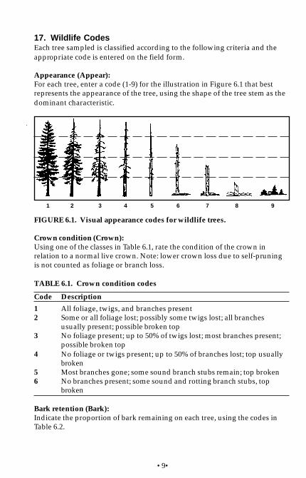
•9•
17. Wildlife CodesEach tree sampled is classified according to the following criteria and theappropriate code is entered on the field form.
Appearance (Appear):For each tree, enter a code (1-9) for the illustration in Figure 6.1 that bestrepresents the appearance of the tree, using the shape of the tree stem as thedominant characteristic.
FIGURE 6.1. Visual appearance codes for wildlife trees.
1 2 3 4 5 6 7 8 9
Crown condition (Crown):Using one of the classes in Table 6.1, rate the condition of the crown inrelation to a normal live crown. Note: lower crown loss due to self-pruningis not counted as foliage or branch loss.
TABLE 6.1. Crown condition codes
Code Description
1 All foliage, twigs, and branches present2 Some or all foliage lost; possibly some twigs lost; all branches
usually present; possible broken top3 No foliage present; up to 50% of twigs lost; most branches present;
possible broken top4 No foliage or twigs present; up to 50% of branches lost; top usually
broken5 Most branches gone; some sound branch stubs remain; top broken6 No branches present; some sound and rotting branch stubs, top
broken
Bark retention (Bark):Indicate the proportion of bark remaining on each tree, using the codes inTable 6.2.

•10•
TABLE 6.2. Bark retention codes
Code Description
1 All bark present2 Bark lost on damaged areas only (< 5% lost)3 Most bark present; bare patches; some bark may be loose (5–25%
lost)4 Bare sections; firm and loose bark remains (26–50% lost)5 Most bark gone; firm and loose bark remains (51–75% lost)6 Trace of bark remains (76–99% lost)7 No bark (100% lost)
Wood condition (Wood):Classify the texture (soundness) of the wood for each tree, using the codes inTable 6.3.
TABLE 6.3 Wood condition codes
Code Description
1 No decay2 Probable limited internal decay and/or deformities3 Wood essentially hard; limited decay4 Wood mostly hard, but decay spreading; soft wood present5 Balance of hard and soft wood; spongy sections6 More soft and spongy wood than hard wood7 No more hard wood; all soft or spongy; powdery sections8 Hollow shell; outer wood mostly hard or firm
Lichen loading (Lichen):Assess all standing live or dead trees for lichen loading on branches that arewithin 4.5 m of the ground or root collar. Assign a rating (0–5) based oncomparison with photos in Estimating the Abundance of Arboreal Forage Lichens(Armleder et al. 1992). A value of 0 indicates no lichens, whether it is a livetree with branches and foliage or a dead tree. If a tree has lichens but noneare below the 4.5 m mark, rate as zero.
Wildlife use:If wildlife are observed using sample trees or if there is evidence of use,record a code for the type of use (activity) in the first column and the user inthe second column (e.g., a feeding bird [FB], nesting amphibian [NA],denning mammal [DM]). If only the activity can be determined, leave thesecond column blank. If no evidence of wildlife use is observed, indicatewith dashes (--).
•11•
Activity:
C Cavity nest May be difficult to detect, but locations are somewhatpredictable, and in season, the begging calls of nestlings are easy todetect; test a tree with a cavity nest by carefully striking it to determine ifthe nest is occupied; if possible, note species in the Comments sectionusing the specific species code (see section “User” below).
• Many woodpeckers prefer nesting in live hardwoods, often under-neath branches.
• Nuthatches and chickadees nest in broken-off standing dead trees, orin broken branch holes, often directly below the breakage pointwhere stem rots have entered the tree and softened the heartwood.
• Cavity nesters have perfectly round or oval nest holes.
• The Pileated Woodpecker and the Common Flicker have oval nestholes.
• Downy Woodpeckers, Chickadees, and Nuthatches have small roundnest holes.
• Brown Creepers have hammock nests under the loose bark.
• Some ducks, owls, and squirrels nest in abandoned woodpeckerholes.
O Open nest Nests of eagles, hawks, owls, and herons are usuallysituated in the upper part or crown of live and dead trees; raptors andherons build large platform-style stick nests.
D Denning/resting May be used by bears, squirrels, bats, marten, fisher,weasels, skunks, and raccoons.
• Bears often hibernate in the hollow trunks of large standing trees,especially western redcedars.
• Entrances to tree dens can be basal or arboreal.
F Feeding Some examples of indicators are:
• Pileated Woodpeckers excavate large rectangular feeding holes.
• Red-breasted and Yellow-bellied Sapsuckers drill horizontal patternsof sap wells.
• Three-toed and Black-backed Woodpeckers scale off bark to feed oninsects.
• Porcupines gnaw on large sections of bark (diagonal tooth marks areoften apparent).
•12•
• Rabbits, hares, and squirrels feed on the base of young trees (squarish“windows” or girdling at the base).
• Squirrels cache cones or leave basal accumulations of cone bracts.
M Mark tree Trees used mostly for communication of territorial bounda-ries and during courtship; examples of indicators include claw marks bygrizzly or black bears, and antler rubbing by deer or elk.
P Perching/roosting Some examples of indicators are:
• Perch trees of aerial foraging and hawking birds are typically tall,with prominent dead branches which provide a good view of thesurrounding area; especially common near riparian edges.
• Plucking spots where raptors feed are identified by “whitewash”and remains of prey in the vicinity.
• Roost trees are often in sheltered locations with natural or excavatedcavities; roosting sites include cavities, hollows, beneath bark, and infoliage.
S Squirrel cache
User:If possible, enter a code identifying the user, as follows:
M = mammalB = birdR = reptileA = amphibian
If a wildlife species using a sample tree can be positively identified, recordthe species code on the Wildlife Habitat Assessment form or record it in theNOTES section of the Site Description Form. Use the six-character codesfound in Appendix 5.1. The first letter identifies the species as mammal (M),bird (B), reptile (R) or amphibian (A); the remaining 4 letters are from thefirst two letters each of the genus and species names, or of the commonnames (mostly in the case of birds).

•13•
APPENDIX 6.1 Tree Species Codes 1
ConifersCommon name Species Code
Cedar Thujawestern redcedar T. plicata Cw
Cypress Chamaecyparisyellow-cedar C. nootkatensis Yc
Douglas-fir PseudotsugaDouglas-fir P. menziesii Fdinterior Douglas-fir P. menziesii var. glauca Fdicoast Douglas-fir P. menziesii var. menziesii Fdc
Fir (Balsam) Abiesamabilis fir A. amabilis Bagrand fir A. grandis Bgsubalpine fir A. lasiocarpa Bl
Hemlock Tsugamountain hemlock T. mertensiana Hmwestern hemlock T. heterophylla Hw
mountain x western hemlock hybrid T. mertensiana x heterophylla HxmJuniper Juniperus
Rocky Mountain juniper J. scopulorum JrLarch Larix
alpine larch L. lyallii Latamarack L. laricina Ltwestern larch L. occidentalis Lw
Pine Pinuswhitebark pine P. albicaulis Palimber pine P. flexilis Pfjack pine P. banksiana Pjlodgepole pine P. contorta Pllodgepole x jack pine hybrid P. x murraybanksiana Pxjshore pine P. contorta var. contorta Plclodgepole pine P. contorta var. latifolia Pliwestern white pine P. monticola Pwponderosa pine P. ponderosa Py
Spruce Piceablack spruce P. mariana SbEngelmann spruce P. engelmannii Sewhite spruce P. glauca SwSitka spruce P. sitchensis Ssspruce hybrid Picea cross Sx
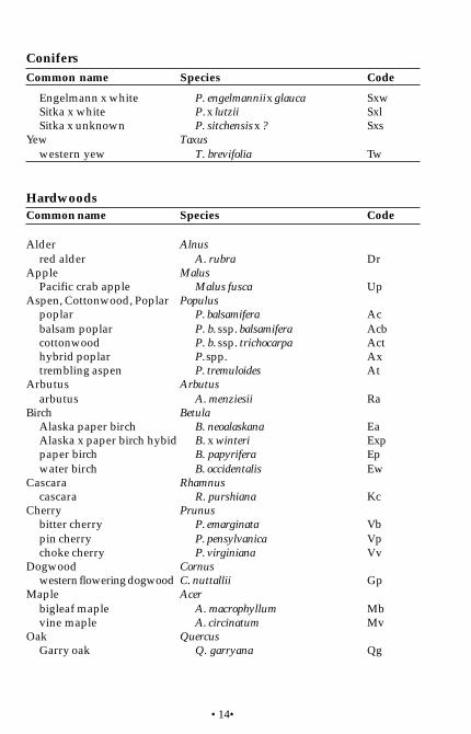
•14•
ConifersCommon name Species Code
Engelmann x white P. engelmannii x glauca SxwSitka x white P. x lutzii SxlSitka x unknown P. sitchensis x ? Sxs
Yew Taxuswestern yew T. brevifolia Tw
HardwoodsCommon name Species Code
Alder Alnusred alder A. rubra Dr
Apple MalusPacific crab apple Malus fusca Up
Aspen, Cottonwood, Poplar Populuspoplar P. balsamifera Acbalsam poplar P. b. ssp. balsamifera Acbcottonwood P. b. ssp. trichocarpa Acthybrid poplar P. spp. Axtrembling aspen P. tremuloides At
Arbutus Arbutusarbutus A. menziesii Ra
Birch BetulaAlaska paper birch B. neoalaskana EaAlaska x paper birch hybid B. x winteri Exppaper birch B. papyrifera Epwater birch B. occidentalis Ew
Cascara Rhamnuscascara R. purshiana Kc
Cherry Prunusbitter cherry P. emarginata Vbpin cherry P. pensylvanica Vpchoke cherry P. virginiana Vv
Dogwood Cornuswestern flowering dogwood C. nuttallii Gp
Maple Acerbigleaf maple A. macrophyllum Mbvine maple A. circinatum Mv
Oak QuercusGarry oak Q. garryana Qg
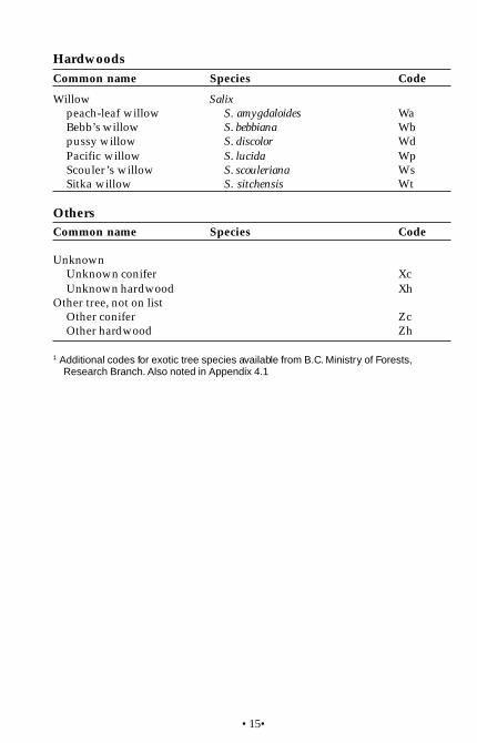
•15•
HardwoodsCommon name Species Code
1 Additional codes for exotic tree species available from B.C. Ministry of Forests,Research Branch. Also noted in Appendix 4.1
Willow Salixpeach-leaf willow S. amygdaloides WaBebb’s willow S. bebbiana Wbpussy willow S. discolor WdPacific willow S. lucida WpScouler’s willow S. scouleriana WsSitka willow S. sitchensis Wt
OthersCommon name Species Code
UnknownUnknown conifer XcUnknown hardwood Xh
Other tree, not on listOther conifer ZcOther hardwood Zh
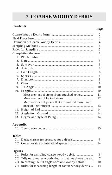
Contents
Coarse Woody Debris Form ...................................................... 2Field Procedure ........................................................................... 3Definition of Coarse Woody Debris.......................................... 4Sampling Methods ..................................................................... 4Rules for Sampling ..................................................................... 5Completing the form .................................................................. 8
1. Plot Number ..................................................................... 82. Date ................................................................................... 83. Surveyor ........................................................................... 84. Azimuth............................................................................ 85. Line Length ...................................................................... 86. Species .............................................................................. 87. Diameter ........................................................................... 88. Class .................................................................................. 89. Tilt Angle .......................................................................... 10
10. Length............................................................................... 10Measurement of stems from attached roots ............... 11Measurement of forked stems ..................................... 12Measurement of pieces that are crossed more thanonce on the transect ...................................................... 13
11. Height of End................................................................... 1412. Angle from Ground......................................................... 1413. Degree and Type of Piling .............................................. 14
Appendix7.1 Tree species codes ............................................................ 15
Tables7.1 Decay classes for coarse woody debris ......................... 97.2 Codes for size of interstitial spaces ................................ 14
Figures7.1 Rules for sampling coarse woody debris ...................... 67.2 Tally only coarse woody debris that lies above the soil 77.3 Recording the tilt angle of coarse woody debris .......... 107.4 Rules for measuring length of coarse woody debris ... 14
7 COARSE WOODY DEBRIS
Page

•2•
Tran
sect
#1
leng
thD
iam
eter
(cm
)S
peci
es
Sam
pled
(0–3
59)
Sur
veyo
r
FS
882
(7)
HR
E 9
8/5
Pro
ject
id.
Azi
mut
ho
f24
m
Leng
th(m
)H
eigh
t of
end
(cm
)
Pile #
Siz
e of
pile
(m
)
wid
thhe
ight
Dia
m(c
m)
Inte
r.sp
ac.
Tree
No. 1
0 0 0 0
2 3 4
05
06
07
08
09
10
11
12
13
14
15
16
17
18
19
20
Class
Tilt
Ang
leA
ngle
grnd
.
COARSE WOODY DEBRISD
ate
ym
d
Plo
t no. Azi
mut
ho
f24
m(0
–359
)S
ampl
ed
Spe
cies
Dia
met
er(c
m)
Leng
th(m
)H
eigh
t of
end
(cm
)
Tran
sect
#2
Class
Tilt
Ang
leA
ngle
grnd
.
1 2 3 4 5 6 7 8 Com
men
ts
Deg
ree
and
Type
of P
iling
(in p
lot b
ound
arie
s)
613
2
3
54
98
107
1112
1
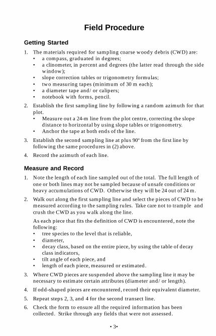
•3•
Field Procedure
Getting Started
1. The materials required for sampling coarse woody debris (CWD) are:• a compass, graduated in degrees;• a clinometer, in percent and degrees (the latter read through the side
window);• slope correction tables or trigonometry formulas;• two measuring tapes (minimum of 30 m each);• a diameter tape and/or calipers;• notebook with forms, pencil.
2. Establish the first sampling line by following a random azimuth for thatplot.• Measure out a 24-m line from the plot centre, correcting the slope
distance to horizontal by using slope tables or trigonometry.• Anchor the tape at both ends of the line.
3. Establish the second sampling line at plus 90o from the first line byfollowing the same procedures in (2) above.
4. Record the azimuth of each line.
Measure and Record
1. Note the length of each line sampled out of the total. The full length ofone or both lines may not be sampled because of unsafe conditions orheavy accumulations of CWD. Otherwise they will be 24 out of 24 m.
2. Walk out along the first sampling line and select the pieces of CWD to bemeasured according to the sampling rules. Take care not to trample andcrush the CWD as you walk along the line.
As each piece that fits the definition of CWD is encountered, note thefollowing:• tree species to the level that is reliable,• diameter,• decay class, based on the entire piece, by using the table of decay
class indicators,• tilt angle of each piece, and• length of each piece, measured or estimated.
3. Where CWD pieces are suspended above the sampling line it may benecessary to estimate certain attributes (diameter and/or length).
4. If odd-shaped pieces are encountered, record their equivalent diameter.
5. Repeat steps 2, 3, and 4 for the second transect line.
6. Check the form to ensure all the required information has beencollected. Strike through any fields that were not assessed.
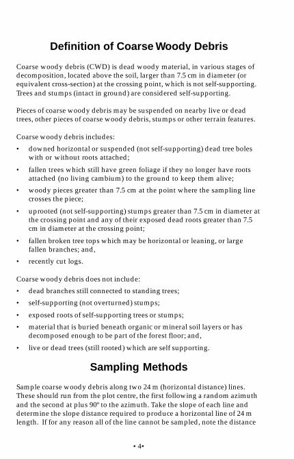
•4•
Definition of Coarse Woody Debris
Coarse woody debris (CWD) is dead woody material, in various stages ofdecomposition, located above the soil, larger than 7.5 cm in diameter (orequivalent cross-section) at the crossing point, which is not self-supporting.Trees and stumps (intact in ground) are considered self-supporting.
Pieces of coarse woody debris may be suspended on nearby live or deadtrees, other pieces of coarse woody debris, stumps or other terrain features.
Coarse woody debris includes:
• downed horizontal or suspended (not self-supporting) dead tree boleswith or without roots attached;
• fallen trees which still have green foliage if they no longer have rootsattached (no living cambium) to the ground to keep them alive;
• woody pieces greater than 7.5 cm at the point where the sampling linecrosses the piece;
• uprooted (not self-supporting) stumps greater than 7.5 cm in diameter atthe crossing point and any of their exposed dead roots greater than 7.5cm in diameter at the crossing point;
• fallen broken tree tops which may be horizontal or leaning, or largefallen branches; and,
• recently cut logs.
Coarse woody debris does not include:
• dead branches still connected to standing trees;
• self-supporting (not overturned) stumps;
• exposed roots of self-supporting trees or stumps;
• material that is buried beneath organic or mineral soil layers or hasdecomposed enough to be part of the forest floor; and,
• live or dead trees (still rooted) which are self supporting.
Sampling Methods
Sample coarse woody debris along two 24 m (horizontal distance) lines.These should run from the plot centre, the first following a random azimuthand the second at plus 90º to the azimuth. Take the slope of each line anddetermine the slope distance required to produce a horizontal line of 24 mlength. If for any reason all of the line cannot be sampled, note the distance
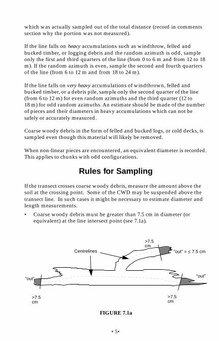
•5•
which was actually sampled out of the total distance (record in commentssection why the portion was not measured).
If the line falls on heavy accumulations such as windthrow, felled andbucked timber, or logging debris and the random azimuth is odd, sampleonly the first and third quarters of the line (from 0 to 6 m and from 12 to 18m). If the random azimuth is even, sample the second and fourth quartersof the line (from 6 to 12 m and from 18 to 24 m).
If the line falls on very heavy accumulations of windthrown, felled andbucked timber, or a debris pile, sample only the second quarter of the line(from 6 to 12 m) for even random azimuths and the third quarter (12 to18 m) for odd random azimuths. An estimate should be made of the numberof pieces and their diameters in heavy accumulations which can not besafely or accurately measured.
Coarse woody debris in the form of felled and bucked logs, or cold decks, issampled even though this material will likely be removed.
When non-linear pieces are encountered, an equivalent diameter is recorded.This applies to chunks with odd configurations.
Rules for Sampling
If the transect crosses coarse woody debris, measure the amount above thesoil at the crossing point. Some of the CWD may be suspended above thetransect line. In such cases it might be necessary to estimate diameter andlength measurements.
• Coarse woody debris must be greater than 7.5 cm in diameter (orequivalent) at the line intersect point (see 7.1a).
Centrelines
>7.5cm
>7.5cm
>7.5cm
“out” = < 7.5 cm
“out”“out”
FIGURE 7.1a
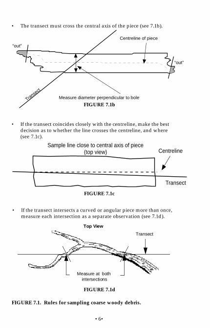
•6•
Transect
Measure diameter perpendicular to bole
Centreline of piece
“out”
“out”
• If the transect coincides closely with the centreline, make the bestdecision as to whether the line crosses the centreline, and where(see 7.1c).
Sample line close to central axis of piece(top view)
Transect
Centreline
• If the transect intersects a curved or angular piece more than once,measure each intersection as a separate observation (see 7.1d).
Measure at both intersections
Transect
Top View
• The transect must cross the central axis of the piece (see 7.1b).
FIGURE 7.1. Rules for sampling coarse woody debris.
FIGURE 7.1b
FIGURE 7.1c
FIGURE 7.1d
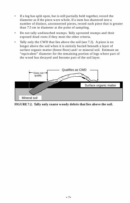
•7•
• If a log has split open, but is still partially held together, record thediameter as if the piece were whole. If a stem has shattered into anumber of distinct, unconnected pieces, record each piece that is greaterthan 7.5 cm in diameter at the point of sampling.
• Do not tally undisturbed stumps. Tally uprooted stumps and theirexposed dead roots if they meet the other criteria.
• Tally only the CWD that lies above the soil (see 7.2). A piece is nolonger above the soil when it is entirely buried beneath a layer ofsurface organic matter (forest floor) and/or mineral soil. Estimate an“equivalent” diameter for the remaining portion of logs where part ofthe wood has decayed and become part of the soil layer.
Does notqualify
Qualifies as CWD
Mineral soil
Surface organic matter
FIGURE 7.2. Tally only coarse woody debris that lies above the soil.

•8•
Completing the Form
Numbered items below refer to circled numbers on the Coarse Woody Debris(CWD) Form shown at the beginning of this section. A recommendedsequence for completing the form is described in "Field Procedure."
1. Plot NumberRecord the plot number and the project identification (Proj. id.) from thetop of the Site Description Form.
2. DateEnter the year (YY), month (MM), and day (DD).
3. SurveyorEnter the first initial and last name of the person(s) collecting CWD data(Survyr).
4. AzimuthRecord the first azimuth (randomly selected) for Transect No. 1, and thesecond at plus 90o to Transect No. 2.
5. Line LengthRecord the distance that was actually sampled (Sampled ___ of 24 m) out ofthe total distance, in the spaces provided.
6. SpeciesRecord code for each piece, using tree species codes found in Appendix 7.1.If the species can not be determined put “X” for unknown, “Xh” forunknown hardwood, or “Xc” for unknown conifer.
7. DiameterRecord the diameter of the piece perpendicular to the bole at the pointwhere the sampling line is considered to intersect the central axis of thepiece. Wrap a diameter tape around the bole, when possible, or use thereverse side of the tape to estimate the diameter. Calipers may also be used,and are often easier when coarse woody debris is in several layers. Measurediameter to the closest 0.1 cm. If the CWD is hollow, estimate the diameterequivalent required to approximate the volume of the remaining wood.
8. ClassAssign a decay class (1 to 5) based on the majority condition of the entirepiece. The five classes used to describe the condition of coarse woodydebris are based primarily upon wood texture, and secondarily on othercharacteristics. See Table 7.1 for descriptions of classes.

•9•
TABLE 7.1. Decay classes for coarse woody debris
Woo
d Te
xtur
e
Por
tion
onG
roun
d
Twig
s <
3 cm
(if o
rigin
ally
pres
ent)
Bar
k
Sha
pe
Inva
ding
Roo
ts
Cla
ss 1
Inta
ct,
hard
Ele
vate
d on
supp
ort
poin
ts
Pre
sent
Inta
ct
Rou
nd
Non
e
Cla
ss 2
Inta
ct,
hard
to
part
ly d
ecay
ing
Ele
vate
d bu
tsa
ggin
g sl
ight
ly
Abs
ent
Inta
ct o
r pa
rtly
mis
sing
Rou
nd
Non
e
Cla
ss 3
Har
d, la
rge
piec
es,
part
lyde
cayi
ng
Sag
ging
nea
rgr
ound
, or
brok
en
Abs
ent
Trac
e
Rou
nd
In s
apw
ood
Cla
ss 4
Sm
all,
bloc
kypi
eces
All
of lo
g on
grou
nd,
sink
ing
Abs
ent
Abs
ent
Rou
nd to
ova
l
In h
eart
woo
d
Cla
ss 5
Man
y sm
all
piec
es,
soft
port
ions
All
of lo
g on
grou
nd,
part
lysu
nken
Abs
ent
Abs
ent
Ova
l
In h
eart
woo
d
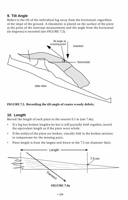
•10•
9. Tilt AngleRefers to the tilt of the individual log away from the horizontal, regardlessof the slope of the ground. A clinometer is placed on the surface of the pieceat the point of the intercept measurement and the angle from the horizontal(in degrees) is recorded (see FIGURE 7.3).
tilt angle atcrossing point
side view
horizontal
transect
10. LengthRecord the length of each piece to the nearest 0.1 m (see 7.4a).
• If a log has broken lengthwise but is still partially held together, recordthe equivalent length as if the piece were whole.
• If the end(s) of the piece are broken, visually fold in the broken sectionsto compensate for the missing parts.
• Piece length is from the largest end down to the 7.5 cm diameter limit.
FIGURE 7.3. Recording the tilt angle of coarse woody debris.
7.5 cm
Length
Transect
FIGURE 7.4a

•11•
Measurement of stems from attached roots:
• For main boles with exposed roots, piece length is measured only downto the root collar (see 7.4b).
• If a root mass is transected, piece length for individual roots (largerthan the minimum diameter) is measured only up to the root collar(see 7.4c).
Transect
Length
Root Collar
FIGURE 7.4c
Root Collar
Transect
Length
7.5 cm
FIGURE 7.4b
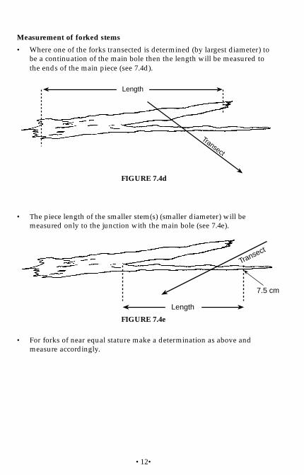
•12•
Measurement of forked stems
• Where one of the forks transected is determined (by largest diameter) tobe a continuation of the main bole then the length will be measured tothe ends of the main piece (see 7.4d).
• The piece length of the smaller stem(s) (smaller diameter) will bemeasured only to the junction with the main bole (see 7.4e).
• For forks of near equal stature make a determination as above andmeasure accordingly.
Transect
Length
Length
Transect
7.5 cm
FIGURE 7.4d
FIGURE 7.4e

•13•
• The full piece length of curved/crooked pieces is measured at bothcrossings (see 7.4g).
FIGURE 7.4. Rules for measuring length of coarse woody debris.
In the same manner as above, record the full piece length twice where thesame piece is crossed by two transects at right angles to each other.
A B Transect
Measurement of pieces that are crossed more than once on the transect:
• Pieces broken but still physically attached are measured as one piece ateach transect point.The length measurement is taken along the centralaxis of the piece (see 7.4f).
A
B
Length
Transect
FIGURE 7.4f
FIGURE 7.4g
Length

•14•
11. Height of Lowest EndThis is the height above ground of the central axis of the lowest end of eachpiece of CWD, measured to the nearest cm. The lowest end is defined as theend of the piece that is in closest contact with the ground, not necessarilythe end that is at the lowest altitude.
12. Angle of GroundAt the transect crossing measure and record the angle of the ground,following the same procedure for determining CWD piece tilt. It may beneccessary to measure the ground angle over a 1 to 2 m (or more) distanceif the surface is irregular.
Record this angle to the nearest degree and indicate whether it is positive ornegative (e.g. -07, +12). When measuring the angle of the ground, face inthe direction that gives a positive tilt angle for the piece of CWD. The angleof ground measured by sighting in that direction may be positive ornegative.
13. Degree and Type of PilingPiles of CWD are important for many wildlife species. Use of the pile isdependent upon interstitial spaces as well as the diameter of pieces and thesize of the pile.
Size of pile:Record the estimated length, width, and height to nearest 0.1 m.
Diameter:Record, to nearest cm, the average diameter of pieces of CWD composingthe pile.
Interstitial Spaces:Using the codes in Table 7.2, estimate of the size of interstitial spaces. Thisnot intended to indicate which species will use the pile.
TABLE 7.5. Codes for size of interstitial spaces.
Code Class Description
s small Most interstitial spaces are the size of, or smallerthan, a squirrel
m medium Most interstitial spaces are the size of a lynx
l large Most interstitial spaces are the size of, or largerthan, the average black bear

•15•
APPENDIX 7.1 Tree Species Codes 1
ConifersCommon name Species Code
Cedar Thujawestern redcedar T. plicata Cw
Cypress Chamaecyparisyellow-cedar C. nootkatensis Yc
Douglas-fir PseudotsugaDouglas-fir P. menziesii Fdinterior Douglas-fir P. menziesii var. glauca Fdicoast Douglas-fir P. menziesii var. menziesii Fdc
Fir (Balsam) Abiesamabilis fir A. amabilis Bagrand fir A. grandis Bgsubalpine fir A. lasiocarpa Bl
Hemlock Tsugamountain hemlock T. mertensiana Hmwestern hemlock T. heterophylla Hw
mountain x western hemlock hybrid T. mertensiana x heterophylla HxmJuniper Juniperus
Rocky Mountain juniper J. scopulorum JrLarch Larix
alpine larch L. lyallii Latamarack L. laricina Ltwestern larch L. occidentalis Lw
Pine Pinuswhitebark pine P. albicaulis Palimber pine P. flexilis Pfjack pine P. banksiana Pjlodgepole pine P. contorta Pllodgepole x jack pine hybrid P. x murraybanksiana Pxjshore pine P. contorta var. contorta Plclodgepole pine P. contorta var. latifolia Pliwestern white pine P. monticola Pwponderosa pine P. ponderosa Py
Spruce Piceablack spruce P. mariana SbEngelmann spruce P. engelmannii Sewhite spruce P. glauca SwSitka spruce P. sitchensis Ssspruce hybrid Picea cross SxEngelmann x white P. engelmannii x glauca Sxw
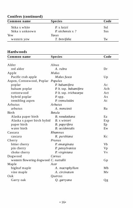
•16•
Conifers (continued)Common name Species Code
Sitka x white P. x lutzii SxlSitka x unknown P. sitchensis x ? Sxs
Yew Taxuswestern yew T. brevifolia Tw
HardwoodsCommon name Species Code
Alder Alnusred alder A. rubra Dr
Apple MalusPacific crab apple Malus fusca Up
Aspen, Cottonwood, Poplar Populuspoplar P. balsamifera Acbalsam poplar P. b. ssp. balsamifera Acbcottonwood P. b. ssp. trichocarpa Acthybrid poplar P. spp. Axtrembling aspen P. tremuloides At
Arbutus Arbutusarbutus A. menziesii Ra
Birch BetulaAlaska paper birch B. neoalaskana EaAlaska x paper birch hybid B. x winteri Exppaper birch B. papyrifera Epwater birch B. occidentalis Ew
Cascara Rhamnuscascara R. purshiana Kc
Cherry Prunusbitter cherry P. emarginata Vbpin cherry P. pensylvanica Vpchoke cherry P. virginiana Vv
Dogwood Cornuswestern flowering dogwood C. nuttallii Gp
Maple Acerbigleaf maple A. macrophyllum Mbvine maple A. circinatum Mv
Oak QuercusGarry oak Q. garryana Qg

•17•
Willow Salixpeach-leaf willow S. amygdaloides WaBebb’s willow S. bebbiana Wbpussy willow S. discolor WdPacific willow S. lucida WpScouler’s willow S. scouleriana WsSitka willow S. sitchensis Wt
OthersCommon name Species Code
UnknownUnknown conifer XcUnknown hardwood Xh
Other tree, not on listOther conifer ZcOther hardwood Zh
Hardwoods (continued)Common name Species Code
1Additional codes for exotic tree species available from B.C. Ministry ofForests, Research Branch. Also noted in Appendix 4.1

•18•

•1•
8 REFERENCES
Armleder, H.M., S.K. Stevenson, and S.D. Walker. 1992. Estimating theabundance of arboreal forage lichens. B.C. Min. For., Victoria,B.C. Land Management Handbook No. 7 (Insert).
Canadian System of Soil Classification. 1998. The Canadian system of soilclassification. Third edition. Soil Classification Working Group,Research Branch, Agriculture Agri-food Canada, Ottawa.
Cannings, R.A. and A.P. Harcombe. (editors). 1990. The vertebrates ofBritish Columbia: scientific and English Names. B.C. Min. ofMunicipal Affairs, Recreation and Culture, and B.C. Min.Environ., Victoria, B.C. Royal British Columbia Museum HeritageRecord No. 20; Wildlife Report No. R24.
Inventory Branch. 1993. Growth and yield: establishment of permanentgrowth samples in natural stands. B.C. Min. For., Victoria, B.C.Forest Inventory Manual.
Green, R., R.L. Trowbridge, and K. Klinka. 1993. Towards a taxonomicclassification of humus forms. Supplement to Forest Science, Vol.39, No. 1, Feb. 1993. Washington, D.C.
Hamilton, E. 1988. A system for the classification of seral ecosystems withinthe Biogeoclimatic Ecosystem Classification system. Firstapproximation. B.C. Min. For. and Lands, Victoria, B.C. ResearchReport RR87004-HQ.
Howes, D.E. and E. Kenk. 1997. Terrain classification system for BritishColumbia. Version 2. B.C. Min. Env., Lands and Parks, MOEManual 10, Victoria, B.C.
Luttmerding, H.A., D.A. Demarchi, E.C. Lea, D.V. Meidinger, and T. Vold.(editors). 1990. Describing ecosystems in the field. Secondedition. B.C. Min. Env., Lands and Parks and B.C. Min. of For.,MOE Manual 11. Victoria, B.C.
Meidinger, D., T. Lee, G.W. Douglas, G. Britton, W. MacKenzie, andH. Qian. 1998. British Columbia plant species codes and selectedattributes. B.C. Min. For., Victoria, B.C. Research Br. Database.
Oliver, C.D., and B.C. Larson, 1990. Forest stand dynamics. McGraw-Hill,New York, N.Y.

Resources Inventory Branch, 1997. Vegetation resources inventory:sampling procedures. B.C. Min. For., Victoria, B.C.
Resources Inventory Committee. 1998. British Columbia Wildlife HabitatRatings Standards. Review Draft. Wildlife InterpretationsSubcommittee. Victoria, B.C.
Resources Inventory Committee. 1997 (in prep). Procedures for wildlifecapability and suitability mapping in British Columbia. ReviewDraft. Wildlife Interpretations Subcommittee. Victoria, B.C.
Resources Inventory Committee: Elements Working Group. 1996. Standard-ized inventory methodologies for components of BritishColumbia’s biodiversity. Prov. of B.C., Victoria, B.C.
Resources Inventory Committee: Terrestrial Ecosystems Group. Standardsfor wildlife habitat capability and suitability ratings in BritishColumbia. Prov. of B.C., Victoria, B.C.
Resources Inventory Committee: Vegetation Inventory Working Group.1995. The British Columbia Land Cover Classification: back-ground and definitions, a working document. Prov. B.C., Victoria,B.C.
VENUS. 1998. VENUS 3.0: Vegetation and Environment data NexUS, data-entry, reporting and analysis tool, version 3. B.C. Min. Environ.and B.C. Min. of For., Victoria, B.C.
Weetman, G.F., E. Ponozzo, M. Jull, and K. Marek. 1990. An assessment ofopportunities for alternative silvicultural systems in the SBS,ICH, and ESSF biogeoclimatic zones of the Prince Rupert ForestRegion. B.C. Min. For., Smithers, B.C. Contract Report.
•2•

•3•

G
PROJECT ID.
MAP SHEET
UTM ZONE
A SPECT
SLOPE
MESO
SLOPE
POSTION
DRAINAGE -MINERAL SOILS
MOISTURE
SUBCLASSES -ORGANIC SOILS
MINERAL SOIL
TEXTURE
ORGANIC SOIL TEXTURE
HUMUS FORM
COARSE FRAGMENT CONTENT
ROOT RESTRICTING LAYER
SURF. ORGANIC HORIZON THICKNESS
TERRAINTERRAIN
TEXTURE
SURFICIAL
MATERIAL
GEOMORPH
PROCESS
SURFACE
EXPRESSION
1
2
1
2
1
2
1
2
ECOSYSTEMBGC UNIT
SITE SERIES
ECOSECTION
SITE MODIFIERS
STRUCTURAL
STAGE
CROWN
CLOSURE %
GROUND INSPECTION FORM
ECOSYSTEM POLYGONSUMMARY
TERRAIN POLYGONSUMMARY
EC3
EC1
EC2
% SS SM ST
TC3
TC1
TC2
% Classification
Vvs
SURV.
PLOT # POLY. #
ELEVATION
DATEY:X:PHOTO
LAT. / NORTH LONG. / EAST
SMR SNR%
m
TC1 TC2 TC3
EC1 EC2 EC3
CrestUpper slope
Toe
Mid slopeLower slope
DepressionLevel
Very rapidlyRapidly
WellMod. wellImperfectly
PoorlyVery poorly
Aqueous
Peraquic
Aquic
Subaquic
Perhumid
Humid
Loamy (SL,L,SCL,FSL)Sandy (LS,S) Silty (SiL,Si)
Clayey (SiCL,CL,SC,SiC,C)
0–40 cm > 40 cmHumicMesicFibric
MullMor Depth cm Type
> 70%35–70%20–35%< 20%
Moder
o
COMPONENT:
COMPONENT:

DOMINANT / INDICATOR PLANT SPECIES
TOTAL %
SPECIES
COMPLETE PARTIAL
Tree MensurationHt. Calculation to DBH
Spp. DBH Top Bot SD SL HD HTHt. toDBH
Total HT
BHAge
Path Y/N
NOTES (site diagram, exposure, gleying, etc.)
SPECIES SPECIESL. L. L.
A: B: C: D:
% % %
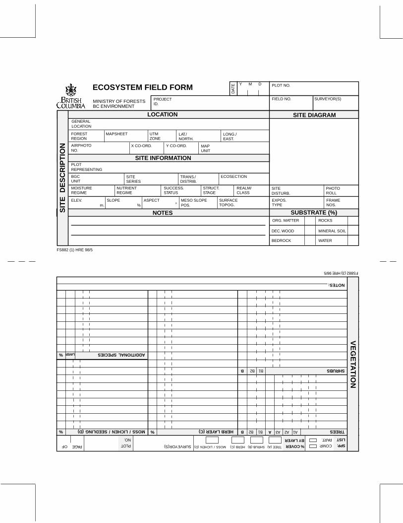
SPP.
LIST
TREE (A)OF
A1A2
SHRUBS
NOTES:
VE
GE
TAT
ION
%
% HERB LAYER (C) TREES
SHRUB (B)HERB (C)MOSS / LICHEN (D)
LAYER
PAGE SURVEYOR(S)
B
B1B2B
B1B2
ADDITIONAL SPECIES
MOSS / LICHEN / SEEDLING (D) % A3A
COMP.
PART.
% COVER
BY LAYERPLOT
NO.
FS882 (3) HRE 98/5
SITE DIAGRAM
FIELD NO. SURVEYOR(S)
SIT
E D
ES
CR
IPT
ION
SITE INFORMATION
NOTES
GENERALLOCATION
UTMZONE
MAPSHEET
Y CO-ORD.
SUBSTRATE (%)ORG. MATTER ROCKS
DEC. WOOD MINERAL SOIL
BEDROCK WATER
EXPOS.TYPE
SITEDISTURB.
ASPECT
PROJECTID.
LAT./NORTH.
m. %o
MESO SLOPEPOS.
SURFACETOPOG.
FORESTREGION
AIRPHOTONO.
PLOTREPRESENTING
BGCUNIT
ELEV.
X CO-ORD. MAPUNIT
LONG./EAST.
SITESERIES
TRANS./DISTRIB.
STRUCT.STAGE
REALM/CLASS
MOISTUREREGIME
SLOPE
PHOTOROLL
FRAMENOS.
ECOSYSTEM FIELD FORM
ECOSECTION
NUTRIENTREGIME
SUCCESS.STATUS
MINISTRY OF FORESTSBC ENVIRONMENT
FS882 (1) HRE 98/5
LOCATION
PLOT NO.
DA
TE Y M D

MENSURATION FORMSURVEYOR(S):TR
EE
#
SPP.DBHTOPBOT.SDSL.HDHT.
HT.TO
DBH
TOTALHT.
BHAGE
SISUP.
BL. C
ON
K
SC
AR
.
CO
NK
F. O
R C
.
F. CR
AC
K
MIS
TLE.
R. B
RA
N.
D. O
R B
.TO
P
TYPESEV.
DAMAGESITESERIES
HEIGHT CALCULATIONS
MEN
SUR
ATION
FS 882 (4) HRE 98/5
NOTESTREE DIAMETER TALLYTREE #TREE # SPP.DBHSPP.DBH
FABRIC
1
2
1 1 1GEOMORPH.PROCESS
DEPTH STRUCTURE vPOSTMYCEL.
AB.FECAL
AB.ROOTS
AB. SIZE COMMENTS (consistency, character, fauna, etc):
DEPTH COLOUR ASP. TEXT.HOR/LAYER
ORGANIC HORIZONS/LAYERS
MINERAL HORIZONS/LAYERS% COARSE FRAGMENTS
C S TOTALGROOTS
AB. SIZESHAPE CLASS KINDSTRUCTURE
GEOLOGY BEDROCK
SOIL CLASS.
TEXTURE
cm cm
ROOTING DEPTH ROOTRESTRICT.LAYER
TYPE
DEPTH
WATER SOURCE
SEEPAGE
DRAINAGE
FLOOD RG.
TERRAIN2
NOTES:
HOR/LAYER
pH
SO
IL D
ES
CR
IPT
ION
R. Z. PART. SIZE
cm
C. F. LITH. SURVEYOR(S)
pHCOMMENTS (mottles, clay films, effervesc., etc):
PLOT NO.
SURFICIALMATERIAL
SURFACEEXPR. 2 2
PROFILE DIAGRAM
HUMUS FORM HYDROGEO.
FS882 (2) HRE 98/5

FS 882 (5) HRE 98/5
Proj. id.
Plot no.
5-letter code
Species
Ssn. FD SH TH
Com
. Habitatfeature C
onf. Distance
(km)F/CL.R. C
om.
Suit.Imp.F/CL.R.
FD SH THDistance
(km)Habitatfeature C
onf.
Imp.
page ofN-hab.feature
type
dst.Surveyor
Date my d
Plot typeHab use / Ssn Plot-in-context
Comments / Notes
WIL
DLI
FE
HA
BIT
AT A
SS
ES
SM
EN
T
Sp. L.R.
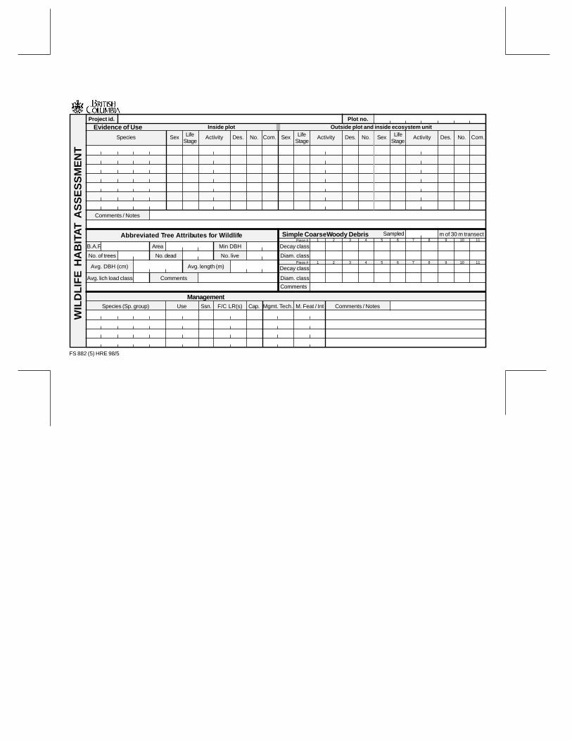
FS 882 (5) HRE 98/5
Project id.Inside plot Outside plot and inside ecosystem unit
Plot no.
Evidence of Use
Species ActivitySex LifeStage
Des. No. Com. ActivitySex LifeStage
Des. No. Com.No.Des.ActivityLifeStage
Sex
Abbreviated Tree Attributes for Wildlife
Comments / Notes
B.A.F.
No. of trees
Avg. DBH (cm)
Avg. lich load class Comments
No. dead
Area
No. live
Min DBH
Avg. length (m)
Simple Coarse Woody Debris Sampled m of 30 m transect
Decay class
Decay class
Diam. class
Diam. class
Comments
Piece #
Piece #
1
1
2
2
3
3
4
4 5
5
6
6
7
7
8 9
8 9
10
10
11
11
ManagementSpecies (Sp. group) Use Ssn. F/C LR(s) Cap. Mgmt. Tech. M. Feat / Int Comments / Notes
WIL
DLI
FE
HA
BIT
AT A
SS
ES
SM
EN
T

FS 882 (6) HRE 98/5
Cro
wn
Bar
kW
ood
Lich
en
Wild
life
use
Cr.
Cla
ss
Botpos(m)
Length Comments
Est
imat
edle
ngth
(m)
M o
r EDBH (cm)TreeNo.
10
0
0
0
2
3
4
0 5
0 6
0 7
0 8
0 9
1 0
1 1
1 2
1 3
1 4
1 5
1 6
1 7
1 8
1 9
2 0
Species
Project id . Plot no. Surveyor
B.A.F (m 2/ha)
Sta
nd/F
all
Rem.Bark(%)
Plot size (m 2) Minimum DBH (cm)
Top(%)
Bot(%)
SlopeDistance
(m)
Heightto
livecrown
(m) App
ear
Wildlife Codes
Date y m d
TR
EE
AT
TR
IBU
TE
S F
OR
WIL
DLI
FE

Transect #1
lengthDiameter
(cm)Species
Sampled(0–359)
Surveyor
FS 882 (7) HRE 98/5
Project id .
Azimuth of24 m
Length(m)
Height ofend (cm)
Pile
# Size of pile (m)
width heightDiam(cm)
Inter.spac.
Tree No.
10
0
0
0
2
3
4
0 5
0 6
0 7
0 8
0 9
1 0
1 1
1 2
1 3
1 4
1 5
1 6
1 7
1 8
1 9
2 0
Cla
ss TiltAngle
Anglegrnd.
CO
AR
SE
WO
OD
Y D
EB
RIS
Date y m d
Plot no.
Azimuth of24 m(0–359) Sampled
Species Diameter(cm)
Length(m)
Height ofend (cm)
Transect #2
Cla
ss TiltAngle
Anglegrnd.
1
2
3
4
5
6
7
8
Comments
Degree and Type of Piling(in plot boundaries)