project deliverables: d13 deliverables: d13.0 scenario comparison and multi-criteria analysis of...
TRANSCRIPT

Project Deliverables: D13.0
Scenario comparison and Multi-Criteria Analysis of Polices and Strategies
Programme name: Energy, Environment and Sustainable Development
Research Programme: 1.1.4. - 4.4.1, 4.1.1
Project acronym: SUTRA
Contract number: EVK4-CT-1999-00013
Project title: Sustainable Urban Transportation
Project Deliverable: D13.0 Scenario comparison and multi-criteria analysis of polices and strategies
Related Work Package:
WP 13 Scenario comparison (all cities)
Type of Deliverable: RE Technical Report
Dissemination level: RES Restricted
Document Author: Sandra Mink, ESS; Jacqueline Rose, MEI
Edited by:
Reviewed by:
Document Version: 1.0
Revision history:
First Availability: 2003 06 01
Final Due Date: 2003 06 30
Last Modification: 2004 06 06
Hardcopy delivered to: Eric Ponthieu DG XII-DI.4 (SDME 4/73) Rue de la Loi, 200 B-1049 Brussels, Belgium

SUTRA Sustainable Urban Transportation
D 13: Scenario comparison and multi-criteria analysis of polices and strategies
Contract number: EVK4-CT-1999-00013
Project title: Sustainable Urban Transportation
Prepared by: Jacqueline Rose Ministry of Environment, Israel 5 Kanfei Nesharim, PO Box 34033 Jerusalem 95464 Phone: +972 2 6553773 Email: [email protected] Sandra Mink Environmental Software and Services Kalkgewerk 1 PO Box 100 A-2352 Gumpoldskirchen – Austria Phone: +43 2252 633 05
Email: [email protected]

WP 13 - Scenario comparison and multi-criteria analysis
1
ENVIRONMENT AND SUSTAINABLE DEVELOPMENT

WP 13 - Scenario comparison and multi-criteria analysis
1
TABLE OF CONTENTS
p.
1. INTRODUCTION 2
2. METHODOLOGY 4
3. ANALYSIS OF ALTERNATIVES 6
4. RULES DEVELOPMENT 10
5. CITY SCENARIO ANALYSIS 17
6. OPTIMISATION EXCERCISE 31
7. RESULTS 35
8. ANNEXES 39
9. REFERENCES 89

WP 13 - Scenario comparison and multi-criteria analysis
2
1. INTRODUCTION 1.1 Objectives The primary objective of WP 13 “Scenario Comparison and Multi-criteria Analysis” is:
• the comparative analysis of the set of scenarios for each city using sustainable city indicators as defined in WP 8 and 10,
• the multi-criteria comparative analysis and selection of a non-dominated set of alternatives and
• the identification of the most promising scenario or small set of candidate scenarios from each test site.
These objectives meet the requirements of the main aim of SUTRA, to develop a consistent and comprehensive approach and planning methodology for the analysis of urban transportation problems, that helps to design strategies for sustainable cities. Each SUTRA city has defined scenarios which examine the current base line situation in terms of transportation and air quality for the year 2000, a do-nothing alternative, and a set of probable development strategies derived from the running of models. These development scenarios reflect changes in terms of demographic, socio-economic, spatial and structural (land-use), and technological aspects for a 30-year horizon (2030). A multi-criteria evaluation methodology has been chosen to analyse the set of scenarios. Based on reference point optimisation, such an analysis makes it possible to rigorously and systematically compare a large set of indicators over a large set of cities and scenarios efficiently and effectively. This should ensure that the overall goal of deriving relevant policy strategies for planning a sustainable city can be achieved. The set of indicators has been pre-defined in WP 8 and 10 according to the DPSIR structure. Indicators defining sustainability are a fundamental part of this analysis as they help to evaluate and measure progress, the distance to a chosen target and failure of plans or their implementation. They are especially important as a tool for cross-comparison over a large set urban scenarios. 1.2 Literature review Defining sustainable development or sustainable cities is the most important element when attempting to identify urban scenarios that best meet the requirements of a sustainable city. Much has been written and discussed on “sustainable development” as a concept, how to define it as an idea and how to achieve it in reality. However the

WP 13 - Scenario comparison and multi-criteria analysis
3
debate focuses mainly on the importance of harmonizing three parameters - economic growth, protection of environment resources, and ensuring social equality - to varying degrees. The most common definition of sustainable development is that used by the Bruntland Commission: “Sustainable development seeks to meet the needs and aspirations of the present without compromising the ability to meet those of the future.” (WCED 1987) Since the coining of this term, many definitions have been developed which try to clarify this broad concept and highlight the need for coordinated planning. New phrases have been created such as sustainable urban development, sustainable transportation, sustainable city. These concepts seek to ensure that the goals of development, growth and economic progress are carried out whilst maintaining the principles of equity, long-term thinking, and ensuring quality of life. The use of indicators has also been deployed to clearly identify those elements which are paramount to ensuring sustainability and enable sustainability to be measured.

WP 13 - Scenario comparison and multi-criteria analysis
4
2. METHODOLGY 2.1 Description of the DSS model
Analysis of the set of scenarios is conducted by a computer based Decision Support System (DSS) for urban traffic and air quality management. A DSS is a flexible model which enables a number of predefined indicators to be selected and weighted. The most sustainable alternative is chosen as the one which most closely fulfils the criteria which were used to define the original sustainable city scenario. Ultimately the DSS improves planning and operational decision making processes. The modelling process involves three stages. 1. Scenario Analysis which required a number of WHAT -- IF questions. Simple
scenario analysis results in a set of results, that is (implicitly or explicitly) compared against a set of objectives or expectations and constraints, such as environmental standards or some minimal requirements for average traffic flow. This has been carried out in WP12.
2. Comparative evaluation or comparative scenario analysis which results in
direct comparison of a set of results, that are explicitly compared against each other and interpreted in terms of improvement or deterioration of performance variables vis a vis the objectives and constraints.
3. A discrete multi-criteria approach to find an efficient strategy (or scenario) that
satisfies all parameters involved in the traffic and environmental management decision processes. The preferences of decision makers can conveniently be defined in terms of a reference point, that indicates one (arbitrary but preferred) location in the solution space.
The data sets describing the scenarios can be displayed in simple scattergrams, using a user defined set of criteria for the (normalized) axes. Along these axes, constraints in terms of minimal and maximal acceptable values of the performance variable in question can be set, leading to a screening and reduction of alternatives. As an implicit reference point, the utopia point can be used. Consequently, the system always has a solution (the feasible alternative nearest to the reference point) that can be indicated and highlighted on the scattergrams (graph 1). Normalizing the solution space in terms of achievement or degree of satisfying each of the criteria between nadir and utopia allows us to find the nearest available Pareto solution efficiently by a simple distance calculation. The selection process is then based on a comparative analysis of the ranking and elimination of (infeasible) alternatives from this set. For spatially distributed and usually dynamic models this process is further complicated, since the number of dimensions (or criteria) that can be used to describe each alternative is potentially very large. Since only a relatively small number of criteria can usefully be compared at any one time it seems important to be able to choose almost any subset of criteria out of this potentially very large set of criteria for further analysis, and modify this selection if required.

WP 13 - Scenario comparison and multi-criteria analysis
5
K.Fedra 2002
Decision SupportDecision SupportDecision SupportReference point approach:Reference point approach:
nadirnadirnadir
utopiautopiautopia
A1A1
A2A2
A3A3
A4A4
betterbetter
efficient efficient pointpoint
criterion 1criterion 1
crite
rion
2cr
iterio
n 2 A5A5
dominateddominated
A6A6
Figure 1: Graphical Representation of the DSS results

WP 13 - Scenario comparison and multi-criteria analysis
6
3. ANALYSIS OF ALTERNATIVES The following section examines the baseline and future scenarios run by each city partner, the indicators gathered as model inputs/outputs, and analyses the range of indicators received. 3.1 Description of the set of scenarios Each city has calibrated a baseline scenario for all models reflecting the current transportation and air quality conditions (for the year 2000). In addition this scenario supplies baseline indicators. Each city partner also runs two types of future scenarios (for the year 2030):
• Common scenarios where all cities run a set of scenarios with pre-defined changes in the set of four parameter – demography, economy, land-use and technolgy. In this instance assumptions are made on the basis of past trends, avaialble forecasts and survey of existing literature, to deduce realistic interval values. This process is described in WP 11 and the list of the four common scenarios is given below.
Table 1. Description of Common Scenarios run by all city partners.
• City Specific Scenarios are defined by each city partner individually. The uniqueness of each city’s individual experience, policies and planning is refelcted in the results.
3.2 List of Indicators Below is the list of sustainable indicators, as defined by Work-Package 8, which will be used for the DSS. The indicators were formulated based on the DPSIR structure and have been compiled by each city. The set of indicators allow analysis and comparisons of the scenarios to be carried out in order to determine those that most closely represent a “sustainable city”.
Dynamic, rich and virtuous
Dynamic, rich and vicious
Virtuous Pensioners City
Vicious Pensioners City
Demographic Increasing Increasing Decreasing Decreasing
Economic Structural Increasing Increasing Decreasing Decreasing
Technological Increasing Decreasing Increasing Decreasing
Land Use Increasing Decreasing Increasing Decreasing

WP 13 - Scenario comparison and multi-criteria analysis
7
Demography number of inhabitants (core/catch.) percentage of population < 18 percentage of population > 64 Land-use structural density functional distribution of urban functions index of mixed use Economy GDP per capita % employment in services % of employment on teleworking Responses: Passenger car occupancy rates (pkm/vkm passenger cars) Share of public transport (% of total pkm) Penetration of alternative technologies (HEV, EV, FCEV) as (% of car fleet) Pressure:** Passenger transport demand (pkm per year) consumption of fossil fuels Emissions of CO2 (tons per year)* NOx (tons per year) VOC (tons per year) ,
CO (tons per year) PM10 (tons per year) **(for private and public transport) State: atmospheric concentrations of pollutants: NOX (annual average conc, pop exp, max CO (pop exp, max) PM10 (annual average conc., pop exp max) O3 (average concentr, IND120) traffic noise levels percentage of population exposed above dB65 crowding (hours in overcrowded public transport) traffic jams (hours spent in traffic jams) Impact: direct costs of transportation system external costs of transportation system mortality caused by pollution by transport number of deaths in a year morbidity caused by pollution by transport number of working days lost in a year number of accidents with personal injuries (days lost?) time losses for congestion •

WP 13 - Scenario comparison and multi-criteria analysis
8
3.3 Analysis of Indicators The list of indicators have been defined according to units, range, distribution They have also been grouped into conceptually relevant categories and assigned relative importance or “weights”. The weighting of indicators for this workpackage is based on “monetizing” the indicators, or giving a financial representation to each indicator. This is not the only way to weight indicators, however it is one of the simplest and enables us to compare a willingness to pay to ensure that sustainability is achieved. Below is an example of six different weighting methodologies (source: Fet, Michelsen, Johnsen 2000)
Unit Eco-
indicator 99 (Damage Control)
EPS (Monetary Valuation
ExternE (monetary
evaluation of external costs)
Political goals
Expert panel
procedures
Deduced from
OECD EST project
Fossil oil kg 0.506 Noise [m2/year] 0.00105 CO2 kg 4.08E-03 0.108 0.0024 0.000000018 NOx kg 2.29 2.13 4 0.000008000 SOx kg 3.27 CO kg 0.331 PM kg 0.19 36 23.95 0.000051600
VOC kg 0.0248 2.14 0.000004350
COMPOSITE TABLE Weighting factors in ELU (Environmental load unit=1 Euro)

WP 13 - Scenario comparison and multi-criteria analysis
9
Sustainable City
• Investment in Transportation
• Efficiency • Affordability • Reliability • Standard of
Living • Safety • Accessibility • Affordability • Exposure • Human Health • Health Effects • Air Pollution • Noise Pollution • Resource
Use/Distribution• Land-use
• GDP/capita • % employed in services • % employed in
teleworking • penetration of alternative
technologies • share of public
transportation • Land-use Index • Traffic jams • Direct Cost of
transportation • Number of work days lost • Number of inhabitants • Structural Density • Passenger car occupancy • Crowding • Passenger transportation
demand • External costs of
transportation • Accidents • Consumption of fossil
fuels • Emissions • Atmospheric
Concentrations • Mortality • Morbidity • Pollution Exposure • Noise
Economic Growth Social Equity Environmental Quality

WP 13 - Scenario comparison and multi-criteria analysis
10
4. RULES DEVELOPMENT 4.1 Introduction
The primary goal of expert systems research is to make expertise available to decision makers and technicians who need answers quickly. Expert systems are systems that provide expert quality advice, diagnoses and recommendations given real world problems. They are meant to solve real problems which normally would require a specialised human expert. Building an expert system therefore first involves extracting the relevant knowledge from the human expert. The most widely used knowledge representation scheme for expert systems is rules.
4.2 Methodology
The objective of a rule-based expert system is to reduce the multidimensionality of the information and to collapse all the data into one dimension so that the different scenarios can be analysed and compared in the same terms. The analysis of the indicators defined in WP 8 in order to develop the rule-based expert system include the following stages: • Grouping of indicators into conceptually relevant categories Based on the primary indicators data aggregating indicators are derived in order to summarize the information. The objective is to obtain an overall evaluation that measures the sustainable transportation performance of the cities. Therefore indicators are classified in three basic categories: economical performances, social performances and environmental quality. As an example for a derived indicator we have transport intensity that is based on the total passenger transport demand, on the public passenger transport demand and on the average distance travelled each year per year, all of them primary indicators. These primary indicators are either direct input from the city partners or are model outputs. The environmental quality category takes into account derived indicators such as pressure on the environment due to transport pollutants emissions
TOTAL PASSENGER TRANSPORT DEMAND PER YEAR (TPTD)
PUBLIC PASSENGER TRANSPORT DEMAND PER YEAR (PPTD)
AVERAGE DISTANCE TRAVELED EACH YEAR PER PERSON (ADTP)
TRA
NSPO
RT
INTEN
SITY

WP 13 - Scenario comparison and multi-criteria analysis
11
(emissions pressure), the actual air quality derived from the peak and average concentrations of pollutants and the consumption of fossil fuels by transportation systems. In the social chapter human health risks are considered. The health risks that the city inhabitants are exposed is derived from transport related illness causing mortality and morbidity, from a stressing factor derived as well considering crowding and traffic jam situations, and from population exposure to pollutant concentrations. Other derived indictors in this category are the transport requirements of the city considering its size, density and age structure, the transport intensity considering passenger demands and the transport safety considered as the danger a person is exposed while using a transportation system analysed in terms of accidents. In the last category, economical performances, examples of derived indicators are living standard, transport efficiency or transport investment. The transport investment is derived considering the direct and the external costs of the transportation system. Finally, the sustainable transport performance is derived taking into account the performance of the city in these three (environmental, social and economical) categories. Using this methodology we have achieved a final overall evaluation of the a urban transportation system considering multiple criteria.
The following table shows in a more graphical way the different levels and diverse derived indicators and how they have been grouped:

WP 13 - Scenario comparison and multi-criteria analysis
12
SUSTAINABLE TRANSPORT PERFORMANCE
ENVIRONMENTAL QUALITY
Concept Sub-concept Indicator Units Source
Total passenger emission in a year [tons] TREM Passenger transport emission per capita in a year [tons/capita] TREM Passenger transport emission per pass-km in a year [tons/pass-km] TREM NO x emissions Percentage of private transport emission over total passenger transport emission in a year
[%] TREM
Total passenger emission in a year [tons] TREM Passenger transport emission per capita in a year [tons/capita] TREM Passenger transport emission per pass-km in a year [tons/pass-km] TREM CO2 emissions Percentage of private transport emission over total passenger transport emission in a year
[%] TREM
Total passenger emission in a year [tons] TREM Passenger transport emission per capita in a year [tons/capita] TREM Passenger transport emission per pass-km in a year [tons/pass-km] TREM VOC emissions Percentage of private transport emission over total passenger transport emission in a year
[%] TREM
Total passenger emission in a year [tons] TREM Passenger transport emission per capita in a year [tons/capita] TREM Passenger transport emission per pass-km in a year [tons/pass-km] TREM CO emissions Percentage of private transport emission over total passenger transport emission in a year
[%] TREM
Total passenger emission in a year [tons] TREM Passenger transport emission per capita in a year [tons/capita] TREM Passenger transport emission per pass-km in a year [tons/pass-km] TREM
Emissions pressure
PM10 emissions Percentage of private transport emission over total passenger transport emission in a year
[%] TREM
Peak concentration [µg/m3] VADIS/OFIS Average annual concentration [µg/m3] ESS Atmospheric [NOx] Above max. threshold [%] ESS Peak concentration [µg/m3] VADIS/OFIS Average annual concentration [µg/m3] ESS Atmospheric [CO] Above max. threshold [%] ESS Peak concentration [µg/m3] VADIS/OFIS Average annual concentration [µg/m3] ESS
Air quality
Atmospheric [PM10] Above max. threshold [%] ESS

WP 13 - Scenario comparison and multi-criteria analysis
13
Atmospheric [O3] Annual average concentration [µg/m3] OFIS IND120 (Index of air quality exceedencies) frequency OFIS
Total consumption of fossil fuels per capita in a year [toe/capita] VISUM Percentage of passenger transport consumption of fossil fuels over total consumption in a year
[toe] MARKAL Fossil fuel consumption
Percentage of private passenger transport consumption in total passenger transport consumption in a year
[%] VISUM
SOCIAL TRANSPORTATION PERFORMANCES
Mortality Number of deaths in a year per capita [number] GDANSK Number of deaths in a year per pass-km [number] GDANSK Percentage of total costs [%] FEEM Morbidity Number of days lost in a year per capita [number] GDANSK
Transport rel. illness
Percentage of total costs [%] FEEM Crowding: hours per capita spent on overcrowded public transports in a year.
[hours/capita] VISUM Stressing factor
Traffic jams: hours per capita spent yearly in traffic jams hours/capita] VISUM PM10: Number of inhabitants under exposure [number] OFIS Nox: Number of inhabitants under exposure [number] OFIS
Health risks
Pop. Pollution exposure
O3: Number of inhabitants under exposure [number] OFIS Number of inhabitants [number] CP Percentage of population under 18 [%] CP
City dynamism
Percentage of population over 64 [%] CP Area [km2] CP Average distance PrT [km] VISUM
Transports requirements
Urban sprawl Average distance PuT [km] VISUM Total passenger transport demand per year [pkm/year] VISUM
Passenger demand Public passenger transport demand per year [pkm/year] VISUM Transport intensity
Traveling distance Average distance traveled each year per person [pkm/capita] VISUM Total number of accidents with personal injuries in a year per capita [number/capita] GDANSK Total number of accidents with personal injuries in a year per pass-km [number/pass-km GDANSK Transport safety Percentage of total costs [%] FEEM
ECONOMICAL PERFORMANCE Penetration rates of EV in car fleet composition [%] FEEM/VISUM Penetration rates of HEV in car fleet composition [%] FEEM/VISUM
New technology penetration
Penetration rates of fuel cell electric vehicles in car fleet composition [%] FEEM/VISUM
Transport efficiency
Use efficiency of Private transport

WP 13 - Scenario comparison and multi-criteria analysis
14
Urban average private car occupancy rate [number] FEEM/VISUM Public transport
trans. systems
Percentage of public transport over total passenger transport [%] FEEM/VISUM Aggregate direct costs of transportation systems in a year, per capita [euros/capita] FEEM Primary costs of
trans. systems Aggregate direct costs of transportation system in a year, per pass-km [euros/pass-km] FEEM Aggregate damage caused by transport in a year, per capita [euros/capita] FEEM
Transportation investment Secondary costs of
trans. systems Aggregate damage caused by transport in a year per pass- km [euros/pass-km] FEEM GDP per capita [euros/capita] CP
Percentage of employment in services over total employment [%] CP Living standard
Percentage of employment on teleworking over total employment [%] CP Total time spent on traveling in a congestion condition in a year per capita
[hours/capita] VISUM Transport reliability
Percentage of total costs [%] FEEM
WP 13 - Scenario comparison and multi-criteria analysis
15
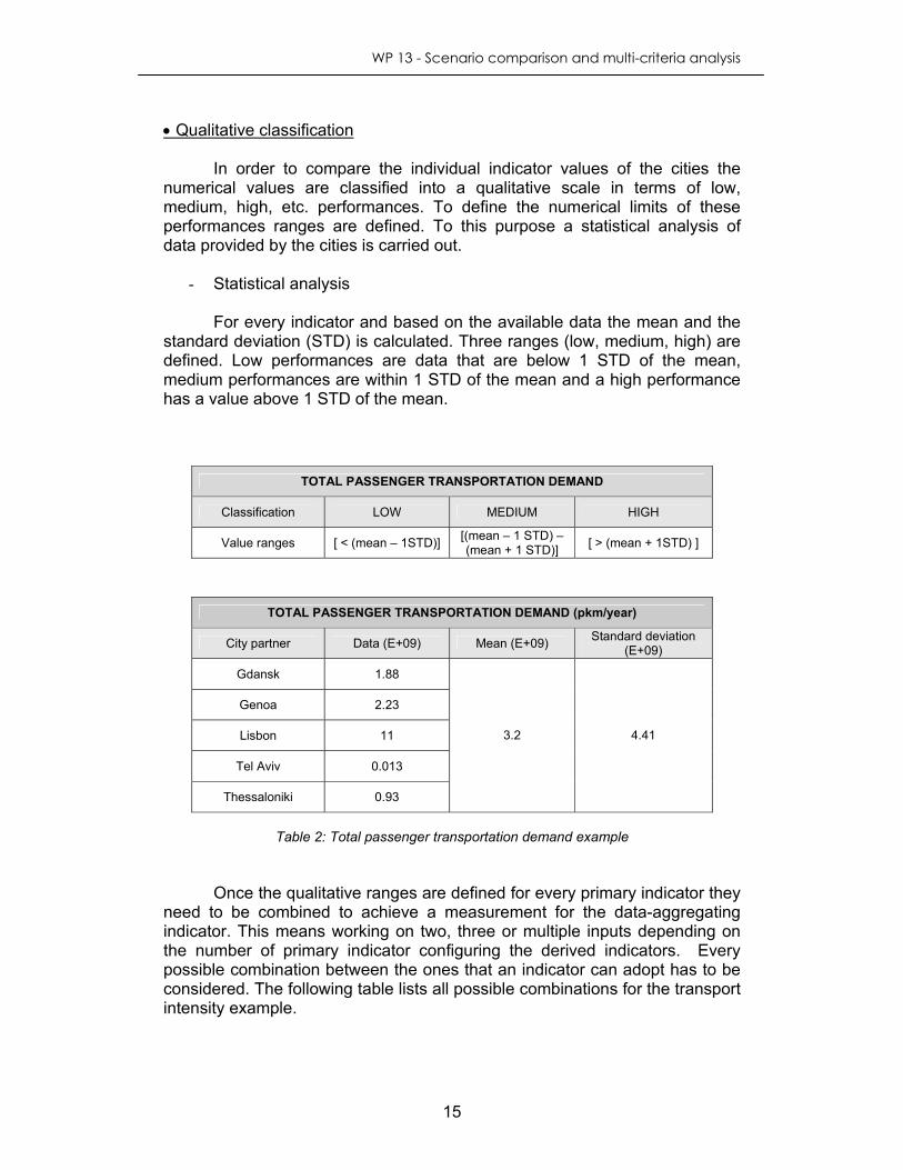
• Qualitative classification In order to compare the individual indicator values of the cities the numerical values are classified into a qualitative scale in terms of low, medium, high, etc. performances. To define the numerical limits of these performances ranges are defined. To this purpose a statistical analysis of data provided by the cities is carried out.
- Statistical analysis For every indicator and based on the available data the mean and the standard deviation (STD) is calculated. Three ranges (low, medium, high) are defined. Low performances are data that are below 1 STD of the mean, medium performances are within 1 STD of the mean and a high performance has a value above 1 STD of the mean.
TOTAL PASSENGER TRANSPORTATION DEMAND
Classification LOW MEDIUM HIGH
Value ranges [ < (mean – 1STD)] [(mean – 1 STD) – (mean + 1 STD)] [ > (mean + 1STD) ]
TOTAL PASSENGER TRANSPORTATION DEMAND (pkm/year)
City partner Data (E+09) Mean (E+09) Standard deviation (E+09)
Gdansk 1.88
Genoa 2.23
Lisbon 11
Tel Aviv 0.013
Thessaloniki 0.93
3.2 4.41
Table 2: Total passenger transportation demand example
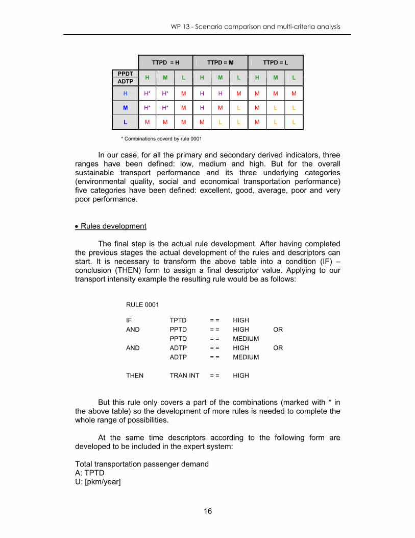
Once the qualitative ranges are defined for every primary indicator they need to be combined to achieve a measurement for the data-aggregating indicator. This means working on two, three or multiple inputs depending on the number of primary indicator configuring the derived indicators. Every possible combination between the ones that an indicator can adopt has to be considered. The following table lists all possible combinations for the transport intensity example.
WP 13 - Scenario comparison and multi-criteria analysis
16
TTPD = H TTPD = M TTPD = L
PPDT ADTP H M L H M L H M L
H H* H* M H H M M M M
M H* H* M H M L M L L
L M M M M L L M L L
* Combinations coverd by rule 0001
In our case, for all the primary and secondary derived indicators, three ranges have been defined: low, medium and high. But for the overall sustainable transport performance and its three underlying categories (environmental quality, social and economical transportation performance) five categories have been defined: excellent, good, average, poor and very poor performance. • Rules development The final step is the actual rule development. After having completed the previous stages the actual development of the rules and descriptors can start. It is necessary to transform the above table into a condition (IF) – conclusion (THEN) form to assign a final descriptor value. Applying to our transport intensity example the resulting rule would be as follows:
RULE 0001
IF TPTD = = HIGH AND PPTD = = HIGH OR PPTD = = MEDIUM AND ADTP = = HIGH OR ADTP = = MEDIUM THEN TRAN INT = = HIGH
But this rule only covers a part of the combinations (marked with * in the above table) so the development of more rules is needed to complete the whole range of possibilities. At the same time descriptors according to the following form are developed to be included in the expert system: Total transportation passenger demand A: TPTD U: [pkm/year]
WP 13 - Scenario comparison and multi-criteria analysis
17
V: Low [ …] V: Medium [ … ] V: High [ … ] R: 0001 / 0002 / 0003 / … Q: What is the total transportation passenger demand measured in pkm in a period of one year? All the results, the developed rules and its descriptors will be included as an annex at the end of the document. 5. CITY SCENARIO ANALYSIS 5.1 Introduction This section analyses the scenario performances of the cities involved in the SUTRA project. The available data provided by the cities has been compared in order to determine which scenario is the most promising one and to identify commonalities and differences between the different performances of the cities. To achieve this objective the indicators data has been analysed grouped in several categories attending to its nature. Each category corresponds to one of the multiple concepts taken into account in the development of the project. The scenarios performances are analysed for transportation demand, pollutant emissions, air quality, consumption of fossil fuels, stressing factors, human health, transportation costs and transport efficiency. The data is analysed to determine the best scenario performance for every city in order to conclude if there is a common trend. At the same time the data is as well analysed to establish which city has the best or worst performance for one given scenario to try to extract conclusions of the reasons of their performances. To facilitate understanding most promising scenarios of every city and for every indicator are highlighted: Green background: best performance within scenarios

WP 13 - Scenario comparison and multi-criteria analysis
18
5.2 Transportation demand
The scenario analysis for the transportation demand shows clearly that all the cities perform in the best way in scenario 3, the virtuous pensioners city. The worst performance goes to scenario 2, dynamic, rich and vicious city. Compared to the baseline the average distance travelled per capita in scenario 3 is lower and in scenario 2 an increment in the distance can be appreciated. Within the case studies, Tel Aviv is the city with the best performance in each scenario whereas Lisbon shows the highest values for scenario 1 and 2 and Gdansk for scenarios 3 and 4.
Gdansk Genoa Lisbon Tel Aviv Thessaloniki
Scenario 0 Total Tr [pkm/yr] 1879E+06 2236E+06 12891E+06 4080E+06 3587E+06 Public Tr [pkm/yr] 771E+06 590E+06 4449E+06 562E+06 598E+06 Average dist. [pkm/cap] 4116.11 3521.02 4805.4 1562.15 4010 Scenario 1 Total trans. [pkm/yr] 2039E+06 3218E+06 14690E+06 6292E+06 3283E+06 Public trans. [pkm/yr] 771E+06 1561E+06 8346E+06 1153E+06 1052E+06 Average dist. [pkm/cap] 3292.88 3241.21 3567.72 1541.29 2348.47 Scenario 2 Total trans. [pkm/yr] 3599E+06 5163E+06 21933E+06 17128E+06 5936E+06 Public trans. [pkm/yr] 771E+06 1211E+06 7283E+06 797E+06 960E+06 Average dist. [pkm/cap] 4939.33 5201.07 5230.74 4195.92 4246.28 Scenario 3 Total trans. [pkm/yr] 1635E+06 1426E+06 6918E+06 1919E+06 1461E+06 Public trans. [pkm/yr] 771E+06 1561E+06 3796E+06 471E+06 5071E+06 Average dist. [pkm/cap] 3292.88 2610.90 3486.23 993.24 2209.66 Scenario 4 Total trans. [pkm/yr] 2237E+06 2233E+06 10222E+06 6837E+06 2665E+06 Public trans. [pkm/yr] 771E+06 540E+06 3313E+06 360E+06 461E+06 Average dist. [pkm/cap] 4939.33 4087.46 5151.37 3539.56 4029.50
Table 3: Scenario results of transportation demand indicators
Total transportation demand per capita
0.00E+00
5.00E+09
1.00E+10
1.50E+10
2.00E+10
2.50E+10
Scena
rio 0
Total tr
ans.
Scena
rio 1
Total tr
ans.
Scena
rio 2
Total tr
ans.
Scena
rio 3
Total tr
ans.
Scena
rio 4
Total tr
ans.
Gdansk
Geneva
Genoa
Lisbon
Tel Aviv
Thessaloniki
Figure 2: Total transportation demand per capita

WP 13 - Scenario comparison and multi-criteria analysis
19
Average distance travelled per capita
9001400
19002400
290034003900
44004900
54005900
Scena
rio 0
Averag
e dist
.
Scena
rio 1
Averag
e dist
.
Scena
rio 2
Averag
e dist
.
Scena
rio 3
Averag
e dist
.
Scena
rio 4
Averag
e dist
.
pkm
per
cap
ita
Gdansk
Geneva
Genoa
Lisbon
Tel Aviv
Thessaloniki
Figure 3: Average distance travelled per capita
Within the case studies, Tel Aviv is the city with the best performance in each scenario whereas Lisbon shows the highest values for scenario 1 and 2 and Gdansk for scenarios 3 and 4. Scenario 3 corresponds to a shrinking and getting older city that is slowly changing towards a high-tech service based economy. It considers as well a fast improvement in transport efficiency and densifying and mixing land uses. It is somewhat obvious that a city with a smaller and a higher number of old age inhabitants will have a lower demand of transportation systems than a growing and younger city because older people tend to have less transport requirements. But it is important for the land use and urban planning to remark that a city with densifying and mixing land uses contributes to reduce the passenger transportations demand in contrast to a city with sprawling and separating ones.
5.3 Pollutant emissions
a. Indicator: Passenger transport emission per capita in a year This analysis has been made taken into account the available data up to the moment. Only the cities of Gdansk, Genoa, Lisbon and Thessaloniki have been considered. Comparing the data of the different scenarios for the cities the best performance scenario for every city has been identified. Scenario 3, virtuous pensioners city, is the most promising one for the cities of Gdansk and Genoa

WP 13 - Scenario comparison and multi-criteria analysis
20
and for Lisbon considering CO2 and PM10 emissions. For Thessaloniki scenario 4, vicious pensioners city, shows the lowest pollutant emission values. Whereas the worst performance, the one with highest emission values, for the considered cities is scenario 2, dynamic, rich and vicious.
Gdansk Genoa Lisbon Thessaloniki Scenario 0
CO2 0.196 0.326 0.562 0.317 NOx 0.0057 0.0015 0.0027 0.0027 VOC 0.0038 0.0065 0.0025 34.84 E-04 CO 5.0968 E-06 0.024 0.0160 156.81 E-04
PM10 9.095 E-05 9.878 E-05 5.81 E-05 Scenario 1
CO2 0.210 0.187 0.425 0.134 NOx 0.0067 0.00012 0.00064 0.0002 VOC 0.0018 0.0013 0.0008 8.70 E-04 CO 5.0967E-06 0.0043 0.0043 29.64 E-04
PM10 3.095 E-05 5.151 E-05 1.14 E-05 Scenario 2
CO2 0.370 0.622 2.233 0.312 NOx 0.0016 0.00038 0.0098 0.0004 VOC 0.0025 0.0032 0.0112 13.74 E-04 CO 5.0968E-06 0.0155 0.0792 57.33 E-04
PM10 9.421 E-05 39.21 E-05 2.79 E-05 Scenario 3
CO2 0.172 0.141 0.348 0.123 NOx 0.0008 9.783 E-05 0.0018 0.0001 VOC 0.0011 0.0010 0.0017 10.66 E-04 CO 5.09636E-06 0.0031 0.0091 29.52 E-04
PM10 2.508 E-05 6.20 E-05 1.06 E-05 Scenario 4
CO2 0.236 0.394 1.304 0.312 NOx 0.0069 0.00027 0.0059 0.0004 VOC 0.0018 0.0028 0.0057 18.87 E-04 CO 5.0968E-06 0.0098 0.0393 69.91 E-04
PM10 7.189 E-05 22.68 E-05 2.57 E-05
Table 4 : Scenario results for passenger transport pollutant emissions per capita
CO2 Passenger transport emissions per capita
0
0.25
0.5
0.75
1
1.25
1.5
CO2 CO2 CO2 CO2 CO2
tons
/yea
r/cap
ita Gdansk
Geneva
Genoa
Lisbon
Tel Aviv
Thessaloniki
Scenario 0 Scenario 1 Scenario 2 Scenario 3 Scenario 4
Figure 4: CO2 Passenger transport emissions per capita

WP 13 - Scenario comparison and multi-criteria analysis
21
NOx and VOC Passenger transport emissions per capita
0
0.002
0.004
0.006
0.008
0.01
0.012
NOx VOC NOx VOC NOx VOC NOx VOC NOx VOC
tons
/yea
r/cap
ita Gdansk
Geneva
Genoa
Lisbon
Tel Aviv
Thessaloniki
Scenario 0 Scenario 1 Scenario 2 Scenario 3 Scenario 4
Figure 5 : NOx and VOC Passenger transport emissions per capita Between the different cities, the city with the highest emission values and therefore the one with worst performance in nearly all pollutant emission values and scenarios is Lisbon. The overall results are similar as the ones obtained analysing the transportation demand because of the correlation between both variables. A lower transportation demand results in a lower use of transportation systems and so pollutant emissions are reduced as well.
5.4 Air quality a. Indicator: Average concentration NOx and CO (ug/m3) Analysing the average concentration of pollutants, NOx and CO, the trend seems to be that the best performing scenario is number 3 with exception of the city of Lisbon. Lisbon values for NOx and CO concentrations reflect lower concentrations for scenario1.

WP 13 - Scenario comparison and multi-criteria analysis
22
Gdansk Genoa Lisbon Thessaloniki Scenario 0
NOx 32000 23.67 1217560 327717 CO 1100000 372.65 9795030 18.64
Scenario 1 NOx 73.32 3.28 11.11 270.28 CO 564119 100.78 81.77 4309.37
Scenario 2 NOx 1.82 22.49 91.83 960.58 CO 929480 810.14 1044.83 10936.39
Scenario 3 NOx 0.65 1.12 12.73 91.83 CO 277282 18.55 86.66 1626.5
Scenario 4 NOx 1.26 4.33 35.11 415.59 CO 542926 132.48 347.91 5774.37
Table 5 : Scenario results for average concentration of NOx and VOC (ug/m3)
NOx Average Concentration
0
50
100
150
200
250
300
350
400
450
NOx NOx NOx NOx
ug/m
3 Gdansk
Genoa
Lisbon
Thessaloniki
Scenario 1 Scenario 2 Scenario 3 Scenario 4
Figure 6 : NOx Average concentration b. Indicator: Above maximum threshold (%) The results for the above maximum threshold values show again that scenario 3 is the most promising one for the cities of Gdansk and Thessaloniki. Genoa’s best performance is attributed to scenario 1 and for the city of Lisbon the different scenarios do not seem to influence the above maximum threshold values for both, NOx and CO, pollutants because the values do not vary.

WP 13 - Scenario comparison and multi-criteria analysis
23
Gdansk Genoa Lisbon Thessaloniki Scenario 0
NOx - 0.05 0.15 0.07 CO - 0.01 0.47 0.08
Scenario 1 NOx 0.18 0.01 0.07 0.06 CO 0.03 0 0.07 0.05
Scenario 2 NOx 0.14 0.01 0.07 0.06 CO 0.18 0.01 0.07 0.06
Scenario 3 NOx 0.14 0.14 0.07 0.04 CO 0.01 0.17 0.07 0.04
Scenario 4 NOx 0.15 0.03 0.07 0.06 CO 0.11 0.01 0.07 0.06
Table 6 : Scenario results for Above max .threshold (%)
NOx Above max Threshold
00.020.040.060.080.1
0.120.140.160.180.2
NOx NOx NOx NOx NOx
%
Gdansk
Genoa
Lisbon
Thessaloniki
Scenario 0 Scenario 1 Scenario 2 Scenario 3 Scenario 4
Figure 7: Above max. threshold values for NOx
5.6 Ozone concentrations The following presented data are the results from the OFIS model runs effectuated for the city cases and scenarios. More detailed information about the model and its methodology can be found in deliverable D.5. The maximum average over threshold (AOT60max), average average over threshold (AOT60ave) and the number of days exceeding the 120 ug/m3 level (E120) have been selected here to make the scenario comparison because they summarize the overall behaviour of the cities in reference to the evolution of the ozone concentrations. AOT60 max: Maximum ppb x hours index in the whole domain AOT60 ave: Average ppb x hours index in the whole domain E120: Number of days exceedance of the 120 µg/m3 value in the whole domain.
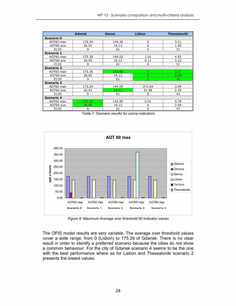
WP 13 - Scenario comparison and multi-criteria analysis
24
Gdansk Genoa Lisbon Thessaloniki Scenario 0
AOT60 max 176.04 144.26 0 3.21 AOT60 ave 26.55 19.13 0 1.95
E120 9 61 0 31 Scenario 1
AOT60 max 175.39 144.02 1.01 4.92 AOT60 ave 26.45 19.12 0.11 3.22
E120 9 61 0 51 Scenario 2
AOT60 max 175.36 143.98 0 3.37 AOT60 ave 26.45 19.13 0 2.08
E120 9 61 0 34 Scenario 3
AOT60 max 175.29 144.05 371.64 3.99 AOT60 ave 26.43 19.11 51.88 2.59
E120 9 61 5 43 Scenario 4
AOT60 max 175.27 143.99 0.01 4.78 AOT60 ave 26.42 19.12 0 2.99
E120 9 61 0 47
Table 7: Scenario results for ozone indicators
AOT 60 max
0.00
50.00
100.00
150.00
200.00
250.00
300.00
350.00
400.00
AOT60 max AOT60 max AOT60 max AOT60 max AOT60 max
ppb
x ho
urs Gdansk
Geneva
Genoa
Lisbon
Tel Aviv
Thessaloniki
Scenario 0 Scenario 1 Scenario 2 Scenario 3 Scenario 4
Figure 8: Maximum Average over threshold 60 indicator values
The OFIS model results are very variable. The average over threshold values cover a wide range, from 0 (Lisbon) to 175.39 of Gdansk. There is no clear result in order to identify a preferred scenario because the cities do not show a common behaviour. For the city of Gdansk scenario 4 seems to be the one with the best performance where as for Lisbon and Thessaloniki scenario 2 presents the lowest values.

WP 13 - Scenario comparison and multi-criteria analysis
25
AOT60 ave
0,00
5,00
10,00
15,00
20,00
25,00
30,00
35,00
40,00
AOT60 ave AOT60 ave AOT60 ave AOT60 ave AOT60 ave
ppb
x ho
urs
GdanskGenevaGenoaLisbonTel AvivThessaloniki
Scenario 0 Scenario 1 Scenario 2 Scenario 3 Scenario 4
Figure 9: Average average over threshold indicator values. Gdansk is the city with the worst performance in the average over threshold maximum and average indicator. Genoa has the highest number of days in the E120 indicator. Lisbon and Tel Aviv seem to be the ones with the best performances if we do not consider scenario 3 of Lisbon that shows a big increase in all three indicators compared to the rest of scenarios.
Number of days exceeding the 120 ug/m3 threshold (E120)
0,00
20,00
40,00
60,00
80,00
100,00
120,00
140,00
160,00
180,00
E120 E120 E120 E120 E120
days
GdanskGenevaGenoaLisbonTel AvivThessaloniki
Scenario 0 Scenario 1 Scenario 2 Scenario 3 Scenario 4
Figure 10: Number of days exceeding 120 ug/m3 threshold
WP 13 - Scenario comparison and multi-criteria analysis
26
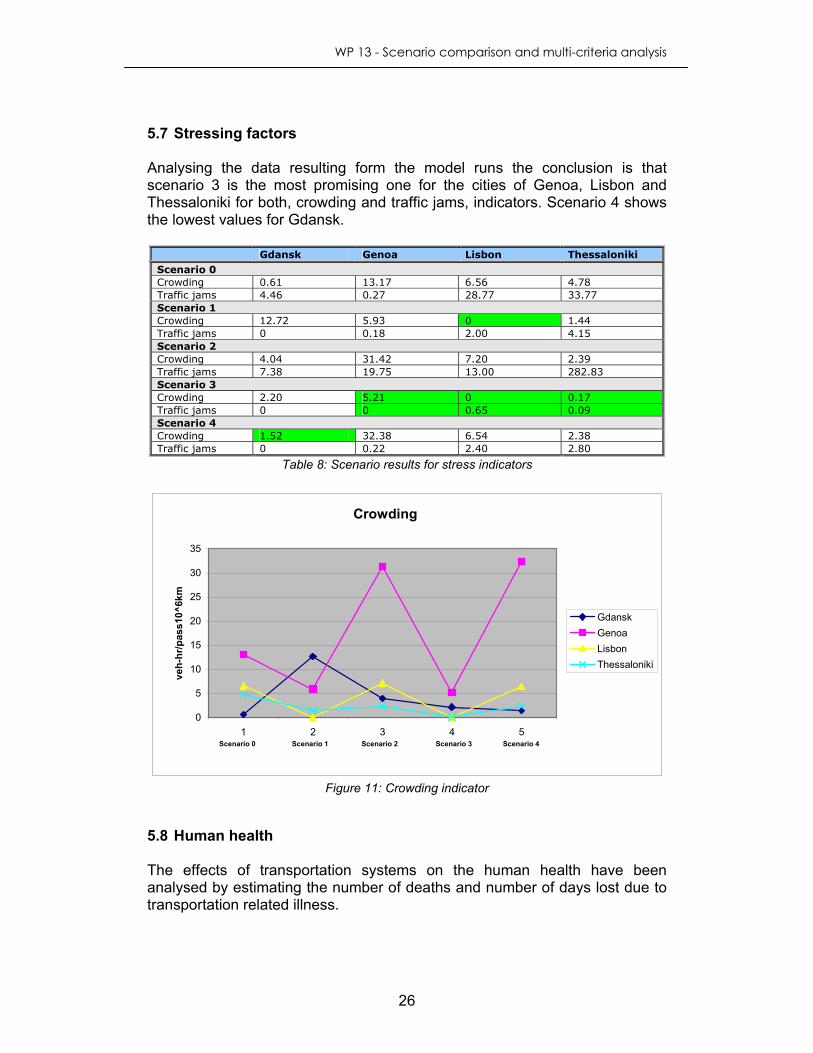
5.7 Stressing factors Analysing the data resulting form the model runs the conclusion is that scenario 3 is the most promising one for the cities of Genoa, Lisbon and Thessaloniki for both, crowding and traffic jams, indicators. Scenario 4 shows the lowest values for Gdansk.
Gdansk Genoa Lisbon Thessaloniki Scenario 0 Crowding 0.61 13.17 6.56 4.78 Traffic jams 4.46 0.27 28.77 33.77 Scenario 1 Crowding 12.72 5.93 0 1.44 Traffic jams 0 0.18 2.00 4.15 Scenario 2 Crowding 4.04 31.42 7.20 2.39 Traffic jams 7.38 19.75 13.00 282.83 Scenario 3 Crowding 2.20 5.21 0 0.17 Traffic jams 0 0 0.65 0.09 Scenario 4 Crowding 1.52 32.38 6.54 2.38 Traffic jams 0 0.22 2.40 2.80
Table 8: Scenario results for stress indicators
Crowding
0
5
10
15
20
25
30
35
1 2 3 4 5
veh-
hr/p
ass1
0^6k
m
GdanskGenoaLisbonThessaloniki
Scenario 0 Scenario 1 Scenario 2 Scenario 3 Scenario 4
Figure 11: Crowding indicator
5.8 Human health The effects of transportation systems on the human health have been analysed by estimating the number of deaths and number of days lost due to transportation related illness.

WP 13 - Scenario comparison and multi-criteria analysis
27
These values have been estimated by a knowledge based system. The objective of the health model is to build system for forecasts the level of mortality and morbidity caused by pollution by transport. The proposed model relies on knowledge-based solutions and the theories of fuzzy sets. A detailed design of fuzzy models takes advantage of the experience of the emitted by the different kinds of vehicles (toxic gases and particles) may cause several human diseases. Data from the project participants have been utilized in tuning of the fuzzy model using knowledge-based rules and membership functions. They include:
• CO total emission [kg/h], methane: Angina - Affects pregnancies, breathing and/or cardiac problems;
• NOx (Nitrogen oxides), Max. Conc. NOx [ug/h], average [ug/h], nonzero Avg.[ug/h],: Bronchitis – Pneumonia, Cancerous diseases
• Mortality caused by pollution by transport [death in a year] • Morbidity caused by pollution by transport [working days lost in a year]
The previously defined variables, fuzzy sets and the membership functions have been set the conditions to build the integrated model using the concept of fuzzy models. Assuming that the model is complete and the rules are continuity and compliance, the number of rules has been depended on the number of input and state variables. If we adopt the rules IF-THEN, then the number of the rules have been completed:
2435*3 === PNR where: R- number of rules N-number of fuzzy sets p-number of input variables The membership function design has been based on clustering methods, where the location of cluster centers of gravity is identified allowing for adjusting the membership functions accordingly.
Example of the description of crisp level for membership functions has been presented in the next figure

WP 13 - Scenario comparison and multi-criteria analysis
28
DESCRIPTION OF THE PARAMETERS
SMALL MEDIUM HIGH110,24 1608694,811 81019504 Max. Conc. NOx [ug/h]1,12 8190,739 1217560 Average [ug/h]7,68 44462,06947 2405390 Nonzero Avg.[ug/h]0,01 0,063 0,15 Above Max. Thres. [%]834,6 5447896,8 56695996 CO Emison (total) [kg/h]
4775,808314 11573 30977,78Mortality [number of
dephs/year]
0,14 0,175 0,23
Morbidity [number of days lost in a year, per capita]
Table 9: Example of the description of the parameters for the fuzzy sets
The suggested fuzzy model treats description of pollutants and examples of morbidity and mortality as a source of knowledge that may be used for carrying out the other ones. It presents the mechanism of the acquisition, implementation and use of knowledge.
The following table presents the results obtained from the health model for the different case studies and the scenarios.
Mortality: number of deaths/year/1000inh
Morbidity: number of days lost per capita
Gdansk Genoa Lisbon Thessaloniki Scenario 0
Mortality 34.16 11.56 11.55 34.63 Morbidity 0.186 0.185 0.23 0.23
Scenario 1 Mortality 43.40 31.20 3.13 8.00 Morbidity 0.23 0.23 0.179 0.173
Scenario 2 Mortality 21.53 13.21 3.13 8.00 Morbidity 0.186 0.178 0.179 0.173
Scenario 3 Mortality 45.49 10.26 6.62 6.62 Morbidity 0.186 0.14 0.179 0.179
Scenario 4 Mortality 45.49 61.18 6.62 6.62 Morbidity 0.186 0.223 0.179 0.179
Table 10: Scenario results for mortality and morbidity
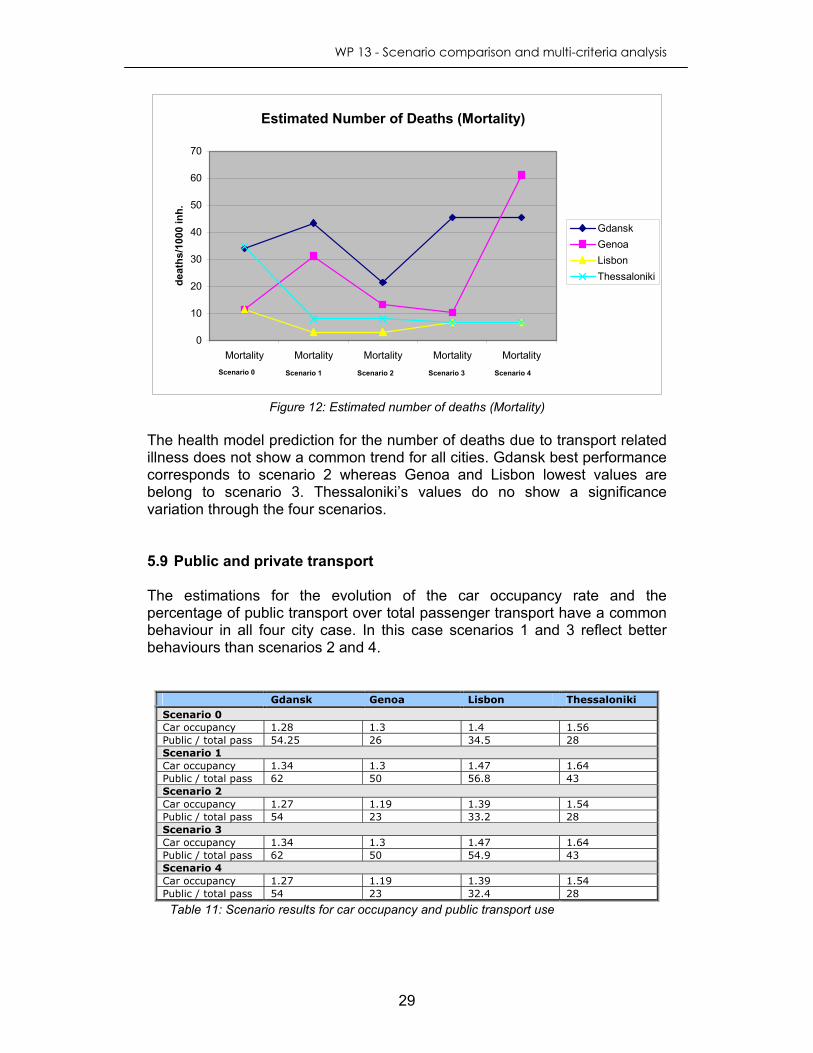
WP 13 - Scenario comparison and multi-criteria analysis
29
Estimated Number of Deaths (Mortality)
0
10
20
30
40
50
60
70
Mortality Mortality Mortality Mortality Mortality
deat
hs/1
000
inh.
GdanskGenoaLisbonThessaloniki
Scenario 0 Scenario 1 Scenario 2 Scenario 3 Scenario 4
Figure 12: Estimated number of deaths (Mortality)
The health model prediction for the number of deaths due to transport related illness does not show a common trend for all cities. Gdansk best performance corresponds to scenario 2 whereas Genoa and Lisbon lowest values are belong to scenario 3. Thessaloniki’s values do no show a significance variation through the four scenarios. 5.9 Public and private transport The estimations for the evolution of the car occupancy rate and the percentage of public transport over total passenger transport have a common behaviour in all four city case. In this case scenarios 1 and 3 reflect better behaviours than scenarios 2 and 4.
Gdansk Genoa Lisbon Thessaloniki Scenario 0 Car occupancy 1.28 1.3 1.4 1.56 Public / total pass 54.25 26 34.5 28 Scenario 1 Car occupancy 1.34 1.3 1.47 1.64 Public / total pass 62 50 56.8 43 Scenario 2 Car occupancy 1.27 1.19 1.39 1.54 Public / total pass 54 23 33.2 28 Scenario 3 Car occupancy 1.34 1.3 1.47 1.64 Public / total pass 62 50 54.9 43 Scenario 4 Car occupancy 1.27 1.19 1.39 1.54 Public / total pass 54 23 32.4 28
Table 11: Scenario results for car occupancy and public transport use

WP 13 - Scenario comparison and multi-criteria analysis
30
Car Occupancy Rate
1
1.1
1.2
1.3
1.4
1.5
1.6
1.7
1 2 3 4 5
Gdansk
Genoa
Lisbon
Thessaloniki
Scenario 0 Scenario 1 Scenario 2 Scenario 3 Scenario 4
Figure 13: Car occupancy rate
Percentage of public transport over total passenger transport
0
10
20
30
40
50
60
70
1 2 3 4 5
%
Gdansk
Genoa
Lisbon
Thessaloniki
Scenario 0 Scenario 1 Scenario 2 Scenario 3 Scenario 4
Figure 14: Percentage of public transport use over total passenger transport
The overall conclusion after having analysed the available data is that
scenario 3 corresponding with a city of pensioners that does not grow and does not change its economic structures but cares about the environment and adopts clean technologies and careful planning is the scenario with best performance on most of the indicators and therefore with the best sustainable performance. A young and growing city moving fast to high-tech services jobs and saving on clean technologies and growing without any landplaning policies into the countryside around like scenario (2) will possibly tend to an unsustainable transportation system.
WP 13 - Scenario comparison and multi-criteria analysis
31
6. OPTIMIZATION EXERCISE - MULTI CRITERIA
ANALYSIS The objective of the multi-criteria analysis is to identify within the different scenarios, the city that has the best performance and identify the factors that lead this city to perform better than the rest in order to extract policy strategies. - Scenarios definition and assumptions The different scenarios defined in WP11 and considered by the city partners are, as already commented in chapter 3, a dynamic, rich and virtuous city, a dynamic, rich and vicious city, a virtuous pensioners city and a vicious pensioners city. The following tables summarize the assumptions taken on the different parameters for every scenario in order to facilitate the posterior understanding of the results. The baseline scenario is calculated for each case study for the year 2000 and used as calibration. Based upon the results of the baseline scenario the percentages of change defined for each scenario are applied and the models are run in order to estimate the possible changes of the pollutant emissions values, atmospheric air concentration or transportation demand for the year 2030 horizon. In addition to these four common scenarios the city partners have selected an individual number of city specific scenarios. The parameter assumptions of the city specific scenarios are chosen within the range defined by the common scenarios taking into account the individual characteristics and development trends foreseen for each city. Scenario 1: Dynamic, rich and virtuous city: A young and growing city moving fast to high-tech services jobs, which cares about the environment and adopts clean technologies and careful planning Scenario 2: Dynamic, rich and vicious city: A young and growing city moving fast to high-tech services jobs, which, however, saves on clean technologies and grows chaotically into the countryside around Scenario 3: Virtuous pensioners city: A city becoming a city of pensioners, it does not grow, it does not change its economic structures, yet, it cares about the environment and adopts clean technologies and careful planning Scenario 4: Vicious pensioner city: A city becoming a city of pensioners, it does not grow, it does not change its economic structures. It does not adopt clean technologies nor careful planning.

WP 13 - Scenario comparison and multi-criteria analysis
32
SCENARIO 1: DYNAMIC, RICH AND VIRTUOUS
1. Population growth p.a. including positive natural (+ 0.5 % pa) and migratory balances (+ 1 % pa)
+ 1.5 %
2.Youth share increases 0.0 %
3. Working age share decreases - 3.0 %
Dem
ogra
phic
ch
anges
4. Old age pensioners share increases + 3.0 %
1.Sector 3 employment share increases + 20.0 %
2. Teleworking share equal to + 50.0 %
3. Mobility rate increases + 25.0 %
Eco
nom
ic
stru
ctura
l ch
anges
4. Goods vehicle transport adding to motorised private transport + 15.0 %
1. Passenger car occupancy rate increases + 5.0 %
2. Passenger urban public transport share increases + 15.0 %
3. Complete knowledge on traffic; network link capacity increases + 10.0 %
Tec
hnolo
gic
al
chan
ges
4. Increases in penetration rate of HEV, EV and FCEV HEV – 13.0 % EV - 7.0 %
FCEV – 7.0 %
Land u
se
chan
ges
1. The average car trip length decreases - 20.0 %
SCENARIO 2: DYNAMIC, RICH AND VICIOUS
1. Population growth p.a. including positive natural (+ 0.5 % pa) and migratory balances (+ 1 % pa)
+ 1.5 %
2.Youth share increases 0.0 %
3. Working age share decreases - 3.0 %
Dem
ogra
phic
ch
anges
4. Old age pensioners share increases + 3.0 %
1.Sector 3 employment share increases + 20.0 %
2. Teleworking share equal to + 50.0 %
3. Mobility rate increases + 25.0 %
Eco
nom
ic
stru
ctura
l ch
anges
4. Goods vehicle transport adding to motorised private transport + 15.0 %
1. Passenger car occupancy rate decreases - 1.0 %
2. Passenger urban public transport share 0.0 %
3. Partial and increasing knowledge on traffic; network link capacity increases
+ 5.0%
Tec
hnolo
gic
al
changes
4. Increases in penetration rate of HEV, EV and FCEV HEV – 7.0 % EV - 4.0 %
FCEV – 3.0 %
Land u
se
changes
1. The average car trip length increases + 20.0 %

WP 13 - Scenario comparison and multi-criteria analysis
33
SCENARIO 3: VIRTUOUS PENSIONERS CITY
1. Population growth p.a. including negative natural and migratory balances (each 0.5 % pa)
- 1.0 %
2.Youth share decreases - 5.0 %
3. Working age share decreases - 10.0 %
Dem
ogra
phic
ch
anges
4. Old age pensioners share increases + 15.0 %
1.Sector 3 employment share increases + 5.0 %
2. Teleworking share equal to + 15.0 %
3. Mobility rate increases + 5.0 %
Eco
nom
ic
stru
ctura
l ch
anges
4. Goods vehicle transport adding to motorised private transport + 25.0 %
1. Passenger car occupancy rate increases + 5.0 %
2. Passenger urban public transport share increases + 15.0 %
3. Complete knowledge on traffic; network link capacity increases + 10.0 %
Tec
hnolo
gic
al
chan
ges
4. Increases in penetration rate of HEV, EV and FCEV HEV – 13.0 % EV - 7.0 %
FCEV – 7.0 %
Land u
se
chan
ges
1. The average car trip length decreases - 20.0 %
SCENARIO 4: VICIOUS PENSIONERS CITY
1. Population growth p.a. including negative natural and migratory balances (each 0.5 % pa)
- 1.0 %
2.Youth share decreases - 5.0 %
3. Working age share decreases - 10.0 %
Dem
ogra
phic
ch
anges
4. Old age pensioners share increases + 15.0 %
1.Sector 3 employment share increases + 5.0 %
2. Teleworking share equal to + 15.0 %
3. Mobility rate increases + 5.0 %
Eco
nom
ic
stru
ctura
l ch
anges
4. Goods vehicle transport adding to motorised private transport + 25.0 %
1. Passenger car occupancy rate decreases - 1.0 %
2. Passenger urban public transport share 0.0 %
3. Partial and increasing knowledge on traffic; network link capacity increases
+ 5.0%
Tec
hnolo
gic
al
changes
4. Increases in penetration rate of HEV, EV and FCEV HEV – 7.0 % EV - 4.0 %
FCEV – 3.0 %
Land u
se
changes
1. The average car trip length increases + 20.0 %

WP 13 - Scenario comparison and multi-criteria analysis
34
The multi-criteria analysis is performed running the Multicriteria DSS software that, with the specified input data, automatically calculates the efficient point as the one closest to utopia.
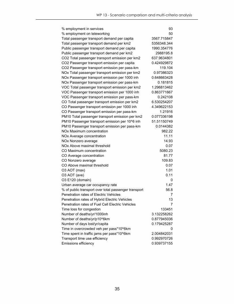
Figure 15: Multicriteria DSS interface To perform one scenario comparison the values of the output model results from WP 12 for this given scenario are used and one file for every city case study is created. For every city case and scenario type, it is necessary to identify as input data:
1. Name of the indicator used for the analysis. 2. Value of the indicator. 3. If the indicator is to maximise or minimise. As an example, one input file should have the following format:
Lisbon Scenario 1
INDICATOR VALUE Inhabitants 4193238 Population under 18 21.5 Population over 64 18
WP 13 - Scenario comparison and multi-criteria analysis
35
% employment in services 93 % employment on teleworking 50 Total passenger transport demand per capita 3567.715847 Total passenger transport demand per km2 5356348.344 Public passenger transport demand per capita 1990.354776 Public passenger transport demand per km2 2988195.8 CO2 Total passenger transport emission per km2 637.9634801 CO2 Passenger transport emission per capita 0.424929872 CO2 Passenger transport emission per pass-km 119.104 NOx Total passenger transport emission per km2 0.97386323 NOx Passenger transport emission per 1000 inh 0.648663428 NOx Passenger transport emission per pass-km 0.181815 VOC Total passenger transport emission per km2 1.296813462 VOC Passenger transport emission per 1000 inh 0.863771667 VOC Passenger transport emission per pass-km 0.242108 CO Total passenger transport emission per km2 6.530254207 CO Passenger transport emission per 1000 inh 4.349622153 CO Passenger transport emission per pass-km 1.21916 PM10 Total passenger transport emission per km2 0.077336198 PM10 Passenger transport emission per 10^6 inh 51.51150749 PM10 Passenger transport emission per pass-km 0.0144382 NOx Maximum concentration 982.22 NOx Average concentration 11.11 NOx Nonzero average 14.93 NOx Above maximal threshold 0.07 CO Maximum concentration 5080.23 CO Average concentration 81.77 CO Nonzero average 109.83 CO Above maximal threshold 0.07 O3 AOT (max) 1.01 O3 AOT (ave) 0.11 O3 E120 (domain) 0 Urban average car occupancy rate 1.47 % of public transport over total passenger transport 56.8 Penetration rates of Electric Vehicles 7 Penetration rates of Hybrid Electric Vehicles 13 Penetration rates of Fuel Cell Electric Vehicles 7 Time loss for congestion 133451 Number of deaths/yr/1000inh 3.132258262 Number of deaths/yr/p10^6km 0.877945036 Number of days lost/yr/capita 0.179425287 Time in overcrowded veh per pass*10^6km 0 Time spent in traffic jams per pass*10^6km 2.004842031 Transport time use efficiency 0.992970726 Emissions efficiency 0.939737155

WP 13 - Scenario comparison and multi-criteria analysis
36
The software allows us to select the indicators of interest interactively out of the complete set of indicators. So that it is possible to analyse the behaviour of the city scenarios focusing on different aspects.
Figure 16: Multicriteria DSS – Selection of criteria
7. RESULTS FROM OPTIMISATION For two selected criteria or indicator the program automatically creates a plot where all the city scenario cases are shown and analysed. Criteria 1 on X axis is displayed against criteria 2 on the Y axis. It is possible to modify the constraints for every criteria. That allows us to increment and reduce the set of dominated and non-dominated points according to our requirements. At the same time we are able to set a new reference point for the criteria if the one given by defaults does not agree with the our ideal (see Figure 17).

WP 13 - Scenario comparison and multi-criteria analysis
37
Figure 17: Multicriteria DSS – Modification of constraints and reference point
WP 13 - Scenario comparison and multi-criteria analysis
38
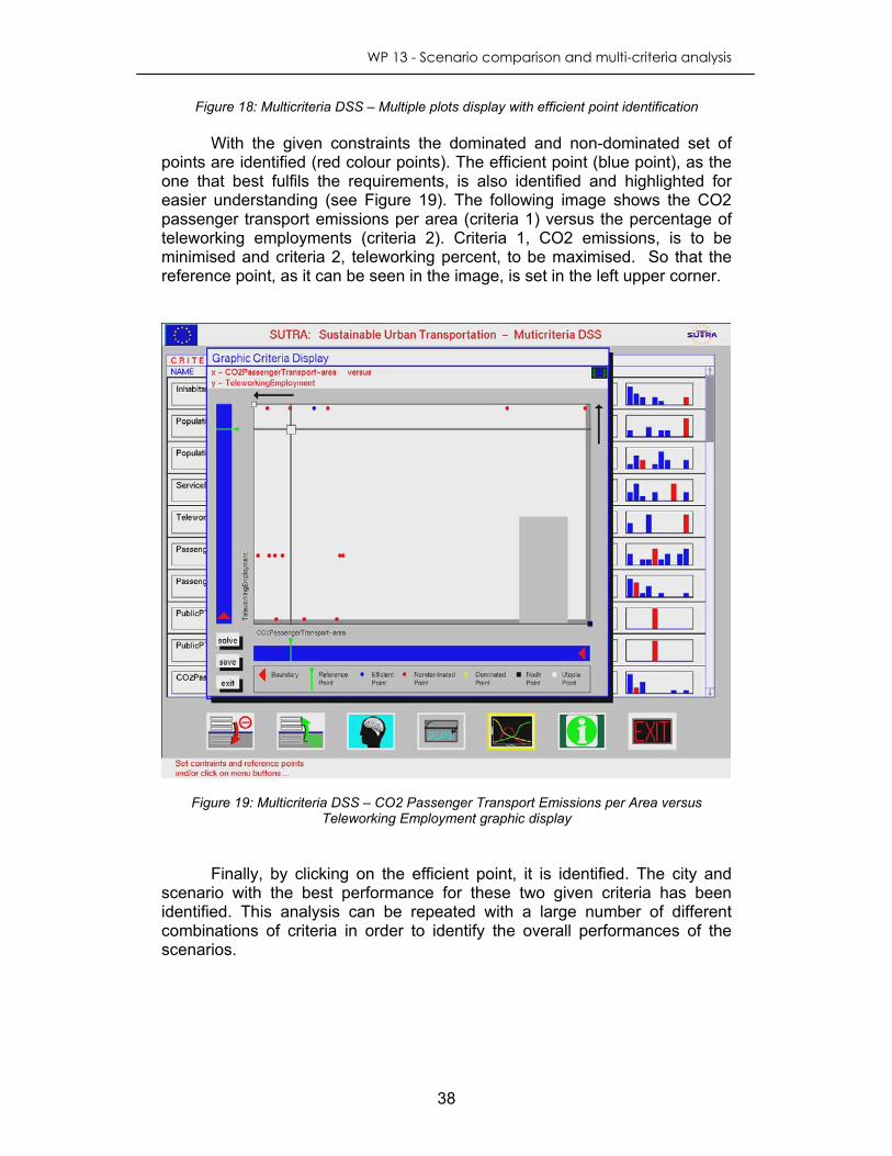
Figure 18: Multicriteria DSS – Multiple plots display with efficient point identification
With the given constraints the dominated and non-dominated set of points are identified (red colour points). The efficient point (blue point), as the one that best fulfils the requirements, is also identified and highlighted for easier understanding (see Figure 19). The following image shows the CO2 passenger transport emissions per area (criteria 1) versus the percentage of teleworking employments (criteria 2). Criteria 1, CO2 emissions, is to be minimised and criteria 2, teleworking percent, to be maximised. So that the reference point, as it can be seen in the image, is set in the left upper corner.
Figure 19: Multicriteria DSS – CO2 Passenger Transport Emissions per Area versus Teleworking Employment graphic display
Finally, by clicking on the efficient point, it is identified. The city and scenario with the best performance for these two given criteria has been identified. This analysis can be repeated with a large number of different combinations of criteria in order to identify the overall performances of the scenarios.

WP 13 - Scenario comparison and multi-criteria analysis
39
8. ANNEXES ANNEX 1. Descriptors developed for the expert system DESCRIPTOR 000 Sustainable_transport_performance A SUSTP T S V excellent / good / average / poor / very_poor R 0237 / 0238 / 0239 / 0240 / 0241 / 0242 / 0243 / 0244 / 0245 / 0246 / 0247 / 0248 / 0249 / 0250 / 0251 / 0252 / 0253 / 0254 / 0255 / 0256 / 0257 Q how would you define the cities overall sustainable transport performance considering factors such as environmental quality, transport impacts on social matters or economical performances? P ENDDESCRIPTOR DESCRIPTOR 001 Environmental_quality A ENVQ T S V excellent / good / average / poor / very_poor R 0224 / 0225 / 0226 / 0227 / 0228 / 0229 / 0230 / 0231 / 0232 / 0233 / 0234 / 0235 / 0236 Q how would you classify the environmental quality of the urban area taking into account factors such as pollutant emissions from transportation systems, air quality derived from atmospheric NOx, PM10, O3 and CO concentrations and fossil fuel consumptions? P ENDDESCRIPTOR DESCRIPTOR 002 Social_transportation_performance A SOCTP T S V excellent / good / average / poor / very_poor R 0191 / 0192 / 0193 / 0194 / 0195 / 0196 / 0197 / 0198 / 0199 / 0200 / 0201 / 0202 / 0203 / 0204 / 0205 / 0206 / 0207 / 0208 / 0209 / 0210 / 0211 / 0212 / 0213 / 0214 / 0215 / 0216 Q how would you define the social performance of the urban transportation system in terms of transport intensity, transport safety, cities transport requirements and human health risks? P ENDDESCRIPTOR DESCRIPTOR 003 Economical_ transportation_performance A ECOTP T S V excellent / good / average / poor / very_poor R 0165 / 0166 / 0167 / 0168 / 0169 / 0170 / 0171 / 0172 / 0173 / 0174 / 0175 / 0176 / 0177 / 0178 / 0179 / 0180 / 0181 / 0182 / 0183 / 0184 / 0185 / 0186 / 0187 / 0188 / 0189 / 0190 Q how would you define the economical performance depending on transport efficiency and new technology penetration, investment and costs of the transportation system, living standard and transport reliability etc.? P ENDDESCRIPTOR DESCRIPTOR 004
WP 13 - Scenario comparison and multi-criteria analysis
40
Emissions_pressure A EPRES T S V high / medium / low R 0001 / 0002 / 0003 / 0004 / 0005 / 0006 / 0007 / 0008 / 0009 / 0010 / 0011 / 0012 / 0013 / 0014 / 0015 / 0016 / 0017 Q how would you classify the pressure derived from the emissions of pollutants such as Nox of transport vehicles on the environment? P ENDDESCRIPTOR DESCRIPTOR 005 Air_quality A AQ T S V high / medium / low R 0217 / 0218 / 0219 / 0220 / 0221 / 0222 / 0223 Q how would you define the air quality based upon the atmospheric concentrations of pollutants such as NOx? P ENDDESCRIPTOR DESCRIPTOR 006 Fossil_fuel_consumption A FFC T S V high / medium / low R 0032 / 0033 / 0034 / 0035 / 0036 / 0037 / 0038 Q how would you classify the consumption of fossil fuels by public and private transportation systems? P ENDDESCRIPTOR DESCRIPTOR 007 NOx_emissions A NOXE T S V high / medium / low R 0001 / 0002 / 0003 / 0004 / 0005 / 0006 / 0007 / 0008 / 0009 / 0010 / 0011 / 0012 / 0013 / 0014 / 0015 / 0016 / 0017 Q how would you classify the amount of NOx emitted to the atmosphere by urban transportation systems? P ENDDESCRIPTOR DESCRIPTOR 008 Atmospheric_NOx_concentration A NOXC T S V high / medium / low R 0018 / 0019 / 0020 / 0021 / 0022 / 0023 / 0024 Q how would you classify the atmospheric concentration of NOx? P ENDDESCRIPTOR DESCRIPTOR 009 Atmospheric_O3_concentration A O3C T S V high / medium / low

WP 13 - Scenario comparison and multi-criteria analysis
41
R Q how would you classify the atmospheric concentration of O3? P ENDDESCRIPTOR DESCRIPTOR 010 Total_passenger_NOx_emission A TPNOXE T S U tons V high [ ] / medium [ ] / low [ ] Q how would you classify the amount of NOx emitted to the atmosphere by the passenger transport system in a year? P ENDDESCRIPTOR DESCRIPTOR 011 Passenger_transport_NOx_emissions_capita A PTNOXE T S U tons/capita V high [ ] / medium [ ] / low [ ] Q how would you classify the amount of NOx emitted by passenger transport systems per capita during one year? P ENDDESCRIPTOR DESCRIPTOR 012 Passenger_transport_NOx_emissions_pass-km A PTNOXEP T S U tons/pass-km V high [ ] / medium [ ] / low [ ] Q how would you classify the amount of NOx emitted by passenger transport systems per passenger and km during one year? P ENDDESCRIPTOR DESCRIPTOR 013 Percentage_private_transport_NOx_emission A PPTNOXE T S U % V high [ ] / medium [ ] / low [ ] Q how would you classify the percentage of NOx emissions due to private transport over the total (private and public) passenger transport NOx emissions? P ENDDESCRIPTOR DESCRIPTOR 014 Peak_NOx_concentration A PNOX T S U µg/m3 V high [ ] / medium [ ] / low [ ] Q how would you classify the measured Nox peak concentration? P ENDDESCRIPTOR DESCRIPTOR 015

WP 13 - Scenario comparison and multi-criteria analysis
42
Average_annual_NOx_concentration A AANOX T S U µg/m3 V high [ ] / medium [ ] / low [ ] Q how would you classify the average atmospheric concentration of NOx in a year? P ENDDESCRIPTOR DESCRIPTOR 016 Average_over _threshold_60 A AOT60 T S U ppb x hours V high [ ] / medium [ ] / low [ ] Q how would you classify the average over threshold value for O3? P ENDDESCRIPTOR DESCRIPTOR 017 Above_max_threshold A AMT T S V high [ ] / medium [ ] / low [ ] Q how would you classify the percentage of Nox concentration above the maximum threshold? P ENDDESCRIPTOR DESCRIPTOR 018 O3_E120 A E120 T days V high [ ] / medium [ ] / low [ ] Q how would you classify the number of days of maximum 8 hours running average O3 concentration exceeding 120 microg/m3? P ENDDESCRIPTOR DESCRIPTOR 019 Total_fossil_fuel_consumption A TFFC T S V high [ ] / medium [ ] / low [ ] Q how would you classify the consumption of fossil fuels by private and public passenger transports per capita during one year? P ENDDESCRIPTOR DESCRIPTOR 020 Percentage_passenger_transport_FF_consumption A PTFFC T S V high [ ] / medium [ ] / low [ ] Q How would you classify the percentage of the total consumption of fossil fuels that is due to the passenger transport in a year? P ENDDESCRIPTOR DESCRIPTOR 021

WP 13 - Scenario comparison and multi-criteria analysis
43
Percentage_private_transport_FF_consumption A PRTFFC T S V high [ ] / medium [ ] / low [ ] Q How would you classify the percentage of fossil fuel consumption over total passenger transport that is due to private passenger transport consumption? P ENDDESCRIPTOR DESCRIPTOR 022 Health_risks A HRISK T S V high [ ] / medium [ ] / low [ ] R 0053 / 0054 / 0055 / 0056 / 0057 / 0058 / 0059 Q How would you define the human health risks a person is exposed taking into account factors like pollutant exposure, transportation stressing factors such as noise, crowding or traffic jams and transport related illness? P ENDDESCRIPTOR DESCRIPTOR 023 Transport_requirements A TREQ T S V high [ ] / medium [ ] / low [ ] R 0109 / 0110 / 0111 / 0112 / 0113 / 0114 / 0115 Q How would you define the city transports requirement considering factors like population dynamism, area extension or urban sprawl, etc.? P ENDDESCRIPTOR DESCRIPTOR 024 Transport_intensity A TINT T S V high [ ] / medium [ ] / low [ ] R 0025 / 0026 / 0027 / 0028 / 0029 / 0030 / 0031 Q how would you classify the transport intensity taking into account factors like passengers demand or travelling distances? P ENDDESCRIPTOR DESCRIPTOR 025 Transport_dangers A TDAN T S V high [ ] / medium [ ] / low [ ] R 0039 / 0040 / 0041 / 0042 / 0043 / 0044 / 0045 Q how would you define the safety conditions of the urban transportation systems in terms of accidents or personal injuries occurred due to its use? P ENDDESCRIPTOR DESCRIPTOR 026 Transport_related_illness A TRILL T S V high [ ] / medium [ ] / low [ ] R 0102 / 0103 / 0104 / 0105 / 0106 / 0107 / 0108

WP 13 - Scenario comparison and multi-criteria analysis
44
Q how would you define occurrence of illness causing morbidity and mortality due to transport air pollution? P ENDDESCRIPTOR DESCRIPTOR 027 Stressing_factor A STRESS T S V high [ ] / medium [ ] / low [ ] R 0074 / 0075 / 0076 / 0077 / 0078 / 0079 / 0080 Q how would you classify the stressing factors such as noise, overcrowded transports or traffic jams the population is exposed? P ENDDESCRIPTOR DESCRIPTOR 028 Population_pollution_exposure A POPEX T S V high [ ] / medium [ ] / low [ ] R 0081 / 0082 / 0083 / 0084 / 0085 / 0086 / 0087 Q how would you classify the population exposure to PM10, Nox or O3 atmospheric concentrations? P ENDDESCRIPTOR DESCRIPTOR 029 Mortality A MORT T S V high [ ] / medium [ ] / low [ ] Q how would you classify mortality due to transport related air pollution in terms of number of deaths? P ENDDESCRIPTOR DESCRIPTOR 030 Morbidity A MORB T S V high [ ] / medium [ ] / low [ ] Q how would you classify morbidity in terms of days lost due to air pollution related illness? P ENDDESCRIPTOR DESCRIPTOR 031 Noise_exposure A NEXP T S V high [ ] / medium [ ] / low [ ] Q how would you classify the number of population exposed to noise above 65 dB(A) over total population? P ENDDESCRIPTOR DESCRIPTOR 032 Crowding A CROW T S
WP 13 - Scenario comparison and multi-criteria analysis
45
V high [ ] / medium [ ] / low [ ] Q how would you classify the hours spent on overcrowded public transport in a year? P ENDDESCRIPTOR DESCRIPTOR 033 Traffic_jams A TJAM T S V high [ ] / medium [ ] / low [ ] Q how would you classify the hours spent yearly in traffic jams P ENDDESCRIPTOR DESCRIPTOR 034 Inhabitants_exposure_PM10 A IEXPPM10 T S V high [ ] / medium [ ] / low [ ] Q how would you classify the number of inhabitants under exposure? P ENDDESCRIPTOR DESCRIPTOR 035 Inhabitants_exposure_NOx A IEXPNOX T S V high [ ] / medium [ ] / low [ ] Q how would you classify the number of inhabitants under exposure? P ENDDESCRIPTOR DESCRIPTOR 036 Inhabitants A INH T S V high [ ] / medium [ ] / low [ ] Q how would you classify the number of inhabitants of the city? P ENDDESCRIPTOR DESCRIPTOR 037 Population_under_18 A PU18 T S U % V high [ ] / medium [ ] / low [ ] Q how would you classify the percentage of the population under 18 years? P ENDDESCRIPTOR DESCRIPTOR 038 Population_over_64 A PO64 T S U % V high [ ] / medium [ ] / low [ ] Q how would you classify the percentage of the population over 64 years? P ENDDESCRIPTOR
WP 13 - Scenario comparison and multi-criteria analysis
46
DESCRIPTOR 039 Area A AREA T S U km2 V high [ ] / medium [ ] / low [ ] Q how would you classify the extension of the city area? P ENDDESCRIPTOR DESCRIPTOR 040 Density A DEN T S V high [ ] / medium [ ] / low [ ] Q how would you classify the population density of the city? P ENDDESCRIPTOR DESCRIPTOR 041 Total_passenger_transport_demand A TPTD T S U pkm/year V high [ ] / medium [ ] / low [ ] Q how would you define the total passenger transport demand for one year? P ENDDESCRIPTOR DESCRIPTOR 042 Public_passenger_transport_demand A PPTD T S U pkm/year V high [ ] / medium [ ] / low [ ] Q how would you define the public transport passenger demand for one year? P ENDDESCRIPTOR DESCRIPTOR 043 Traveling_distance A TDIS T S U pkm/capita V high [ ] / medium [ ] / low [ ] Q how would you define the average distance travelled each year by a person? P ENDDESCRIPTOR DESCRIPTOR 044 Accidents_capita A ACCC T S V high [ ] / medium [ ] / low [ ] Q how would you define the total number of accidents with personal injuries occurred during one year per capita? P ENDDESCRIPTOR

WP 13 - Scenario comparison and multi-criteria analysis
47
DESCRIPTOR 045 City_dynamism A CDYN T S V high [ ] / medium [ ] / low [ ] R 0088 / 0089 / 0090 / 0091 / 0092 / 0093 / 0094 Q how would you define the dynamism of the city considering its number of inhabitants and the population age structure? P ENDDESCRIPTOR DESCRIPTOR 046 Urban sprawl A USPR T S V high [ ] / medium [ ] / low [ ] R Q how would you define the urban sprawl of the city? P ENDDESCRIPTOR DESCRIPTOR 047 Transport_efficiency A TEFF T S V high [ ] / medium [ ] / low [ ] R 0116 / 0117 / 0118 / 0119 / 0120 / 0121 / 0122 Q how would you define the performance of the transportation systems in terms of efficiency considering factors like new technology penetration or the use efficiency of public and private transports? P ENDDESCRIPTOR DESCRIPTOR 048 Transportation_investment A TINV T S V high [ ] / medium [ ] / low [ ] R 0123 / 0124 / 0125 / 0126 / 0127 / 0128 / 0129 Q how would you define the monetary investment in transportation systems considering primary (direct) and secondary (external) costs? P ENDDESCRIPTOR DESCRIPTOR 049 Living_standard A LSTA T S V high [ ] / medium [ ] / low [ ] R 0144 / 0145 / 0146 / 0147 / 0148 / 0149 / 0150 Q how would you define the city living standard? P ENDDESCRIPTOR DESCRIPTOR 050 Transport_reliability A TREL T S V high [ ] / medium [ ] / low [ ] R 0130 / 0131 / 0132 / 0133 / 0134 / 0135 / 0136
WP 13 - Scenario comparison and multi-criteria analysis
48
Q how would you define the transport reliability in terms of time loss due to congestions? P ENDDESCRIPTOR DESCRIPTOR 051 New_technology_penetration A NTECHP T S V high [ ] / medium [ ] / low [ ] R 0046 / 0047 / 0048 / 0049 / 0050 / 0051 / 0052 Q how would you define the penetration of new technologies like electric, hybrid electirc or fuel cell electric vehicles in the car fleet composition? P ENDDESCRIPTOR DESCRIPTOR 052 Use_efficiency_transport_systems A UETS T S V high [ ] / medium [ ] / low [ ] R 0060 / 0061 / 0062 / 0063 / 0064 / 0065 / 0066 Q how would you define the use efficiency of transport systems considering the sharing of private transports and the using rate of public transport systems? P ENDDESCRIPTOR DESCRIPTOR 053 Primary_costs A PCOST T S V high [ ] / medium [ ] / low [ ] Q how would you classify the primary (direct) costs of the transportation system including tasks like cleaning, maintenance and construction of infrastuctures? P ENDDESCRIPTOR DESCRIPTOR 054 Secondary_costs A SCOST T S V high [ ] / medium [ ] / low [ ] Q how would you classify the secondary (external) in terms of aggregated damage caused by transport? P ENDDESCRIPTOR DESCRIPTOR 055 Penetration_rate_EV A PREV T S U % V high [ ] / medium [ ] / low [ ] Q how would you classify the penetration rate of electronic vehicles in the car fleet composition? P ENDDESCRIPTOR DESCRIPTOR 056 Penetration_rate_HEV A PRHEV

WP 13 - Scenario comparison and multi-criteria analysis
49
T S U % V high [ ] / medium [ ] / low [ ] Q how would you classify the penetration rate of hybrid electronic vehicles in the car fleet composition? P ENDDESCRIPTOR DESCRIPTOR 057 Penetration_rate_FCEV A PRFCEV T S U % V high [ ] / medium [ ] / low [ ] Q how would you classify the penetration rate of fuel cell electronic vehicles in the car fleet composition? P ENDDESCRIPTOR DESCRIPTOR 058 Average_car_occupancy_rate A ACOR T S V high [ ] / medium [ ] / low [ ] Q how would you classify the average car occupancy rate of private transport? P ENDDESCRIPTOR DESCRIPTOR 059 Percentage_PuT_use A PPTU T S U % V high [ ] / medium [ ] / low [ ] Q how would you define the percentage of total passenger transport due to public transport use? P ENDDESCRIPTOR DESCRIPTOR 060 Gross_domestic_product A GDP A T S U euros/capita V high [ ] / medium [ ] / low [ ] Q how would you define the gross domestic product per capita of the city? P ENDDESCRIPTOR DESCRIPTOR 061 Percentage_employment_services A PEMS T S U % V high [ ] / medium [ ] / low [ ] Q how would you classify the percentage of employment in the service branch over total employment? P ENDDESCRIPTOR

WP 13 - Scenario comparison and multi-criteria analysis
50
DESCRIPTOR 062 Percentage_employment_teleworking A PEMT T S U % V high [ ] / medium [ ] / low [ ] Q how would you classify the percentage of employment on teleworking over total employment? P ENDDESCRIPTOR DESCRIPTOR 063 Time_travelling_congestion A TTC T S U hours/capita V high [ ] / medium [ ] / low [ ] Q how would you classify the total time spent on travelling in a congestion condition per capita in a year? P ENDDESCRIPTOR DESCRIPTOR 064 Time_congestion_PTC A TCPTC T S U % V high [ ] / medium [ ] / low [ ] Q how would you classify the percentage of total (direct and external) costs due to time spent in congestions? P ENDDESCRIPTOR DESCRIPTOR 065 O3_maxCave A MCAVE T S U microg/m3 V high [ ] / medium [ ] / low [ ] Q how would you define the maximum value of the ozone concentration that is calculated for the considered city area? P ENDDESCRIPTOR DESCRIPTOR 066 O3_aveCave A ACAVE T S U microg/m3 V high [ ] / medium [ ] / low [ ] Q how would you define the average value of the ozone concentration that is calculated for the considered city area? P ENDDESCRIPTOR DESCRIPTOR 067 O3_maxIND120 A MAX120 T S

WP 13 - Scenario comparison and multi-criteria analysis
51
U microg/m3 V high [ ] / medium [ ] / low [ ] Q how would you define the maximum value of the IND120 index, calculated as the number of days with maximum 8 hours running average ozone concentration exceeding 120 microg/m3, that is calculated for the considered city area ? P ENDDESCRIPTOR DESCRIPTOR 068 O3_aveIND120 A AVE120 T S U microg/m3 V high [ ] / medium [ ] / low [ ] Q how would you define the average value of the IND120 index, calculated as the number of days with maximum 8 hours running average ozone concentration exceeding 120 microg/m3, that is calculated for the considered city area ? P ENDDESCRIPTOR DESCRIPTOR 069 O3_minIND120 A MIN120 T S U microg/m3 V high [ ] / medium [ ] / low [ ] Q how would you define the minimum value of the IND120 index, calculated as the number of days with maximum 8 hours running average ozone concentration exceeding 120 microg/m3, that is calculated for the considered city area? P ENDDESCRIPTOR ANNEX 2. Rules developed for the expert system
NOx emissions RULE 0001 IF TPNOXE = = H AND PPTNOXE = = H [AND PTNOXE = = H OR PTNOXEP = = H] OR [AND PTNOXE = = M OR AND PTNOXEP = = M] THEN NOXE = H ENDRULE RULE 0002 IF TPNOXE = = M AND PPTNOXE = = H [AND PTNOXE > = M AND PTNOXEP = = H] OR [AND PTNOXE = = H AND PTNOXEP = = M] THEN NOXE = H ENDRULE RULE 0003
WP 13 - Scenario comparison and multi-criteria analysis
52
IF PTNOXE = = H AND PTNOXEP = = H [AND TPNOXE > = M AND PPTNOXE = = M] OR [AND TPNOXE = = H AND PPTNOXE = = L] OR [AND TPNOXE = = L AND PPTNOXE = = H] THEN NOXE = H ENDRULE RULE 0004 IF TPNOXE = = H AND PPTNOXE = = M [AND PTNOXE > = M AND PTNOXEP = = H] OR [AND PTNOXE = = H AND PTNOXEP = = M] THEN NOXE = H ENDRULE RULE 0005 IF TPNOXE = = L AND PPTNOXE = = L [AND PTNOXE = = L OR PTNOXEP = = L] OR [AND PTNOXE = = M AND PTNOXEP = = M] THEN NOXE = L ENDRULE RULE 0006 IF TPNOXE = = M AND PPTNOXE = = L [AND PTNOXE = = L AND PTNOXEP < = M] OR [AND PTNOXE = = M AND PTNOXEP = = L] THEN NOXE = L ENDRULE RULE 0007 IF TPNOXE = = L AND PPTNOXE = = M [AND PTNOXE = = L AND PTNOXEP < = M] OR [AND PTNOXE = = M AND PTNOXEP = = L] THEN NOXE = L ENDRULE RULE 0008 IF PTNOXE = = L AND PTNOXEP = = L [AND TPNOXE = = L AND PPTNOXE = = H] OR [AND TPNOXE = = M AND PPTNOXE = = M] OR [AND TPNOXE = = L AND PPTNOXE = = L]

WP 13 - Scenario comparison and multi-criteria analysis
53
THEN NOXE = L ENDRULE RULE 0009 IF TPNOXE = = M AND PPTNOXE = = M [AND PTNOXE ! = H AND PTNOXEP ! = H] OR [AND PTNOXE ! = L AND PTNOXEP ! = L] THEN NOXE = M ENDRULE RULE 0010 IF TPNOXE = = L AND PPTNOXE = = H [AND PTNOXE ! = H AND PTNOXEP ! = H] OR [AND PTNOXE ! = L AND PTNOXEP ! = L] THEN NOXE = M ENDRULE RULE 0011 IF TPNOXE = = H AND PPTNOXE = = L [AND PTNOXE ! = H AND PTNOXEP ! = H] OR [AND PTNOXE ! = L AND PTNOXEP ! = L] THEN NOXE = M ENDRULE RULE 0012 IF TPNOXE = = H AND PPTNOXE = = H [AND PTNOXE = = L OR PTNOXEP = = L] OR [AND PTNOXE = = M AND PTNOXEP = = M] THEN NOXE = M ENDRULE RULE 0013 IF TPNOXE = = H AND PPTNOXE = = M [AND PTNOXE = = L OR PTNOXEP = = L] OR [AND PTNOXE = = M AND PTNOXEP = = M] THEN NOXE = M ENRULE RULE 0014 IF TPNOXE = = H AND PPTNOXE = = H [AND PTNOXE = = L AND PTNOXEP < = M] OR [AND PTNOXE = = M AND PTNOXEP = = L]

WP 13 - Scenario comparison and multi-criteria analysis
54
THEN NOXE = M ENDRULE RULE 0015 IF TPNOXE = = L AND PPTNOXE = = M [AND PTNOXE = = H OR PTNOXEP = = H] OR [AND PTNOXE = = M AND PTNOXEP = = M] THEN NOXE = M ENDRULE RULE 0016 IF TPNOXE = = M AND PPTNOXE = = L [AND PTNOXE = = H OR PTNOXEP = = H] OR [AND PTNOXE = = M AND PTNOXEP = = M] THEN NOXE = M ENDRULE RULE 0017 IF TPNOXE = = L AND PPTNOXE = = L [AND PTNOXE = = H AND PTNOXEP > = M] OR [AND PTNOXE = = M AND PTNOXEP = = H] THEN NOXE = M ENDRULE Atmospheric Nox concentration RULE 0018 IF AANOX = = H AND EXNOX = = H THEN NOXC = H ENDRULE RULE 0019 IF PNOX = = H AND AANOX = = H OR EXNOX = = H THEN NOXC = H ENDRULE RULE 0020 IF AANOX = = L AND EXNOX = = L THEN NOXC = L ENDRULE RULE 0021 IF PNOX = = L AND AANOX = = L OR EXNOX = = L THEN NOXC = L
WP 13 - Scenario comparison and multi-criteria analysis
55
ENDRULE RULE 0022 IF PNOX = = H [AND AANOX = = M AND EXNOX > = M] OR [AND AANOX = = L AND EXNOX = = M] THEN NOXC = M ENDRULE RULE 0023 IF PNOX = = M [AND AANOX < = M AND EXNOX < = M] OR [AND AANOX > = M AND EXNOX > = M] THEN NOXC = M ENDRULE RULE 0024 IF PNOX = = L [AND AANOX = = M AND EXNOX < = M] OR [AND AANOX = = H AND EXNOX = = M] THEN NOXC = M ENDRULE Transport intensity RULE 0025 IF PPTD = = H AND ADT = = H THEN TINT = H ENDRULE RULE 0026 IF TPTD = = H AND PPTD = = H OR ADT = = H THEN TINT = H ENDRULE RULE 0027 IF PPTD = = L AND ADT = = L THEN TINT = L ENDRULE RULE 0028 IF TPTD = = L AND PPTD = = L OR ADT = = L THEN TINT = L ENDRULE RULE 0029

WP 13 - Scenario comparison and multi-criteria analysis
56
IF TPTD = = H [AND PPTD = = M AND ADT > = M] OR [AND PPTD = = L AND ADT = = M] THEN TINT = M ENDRULE RULE 0030 IF TPTD = = M [AND PPTD < = M AND ADT < = M] OR [AND PPTD > = M AND ADT > = M] THEN TINT = M ENDRULE RULE 0031 IF TPTD = = L [AND PPTD = = M AND ADT < = M] OR [AND PPTD = = H AND ADT = = M] THEN TINT = M ENDRULE Fossil fuel consumption RULE 0032 IF PTFFC = = H AND PRTFFC = = H THEN FFC = H ENDRULE RULE 0033 IF TFFC = = H AND PTFFC = = H OR PRTFFC = = H THEN FFC = H ENDRULE RULE 0034 IF PTFFC = = L AND PRTFFC = = L THEN FFC = L ENDRULE RULE 0035 IF TFFC = = L AND PTFFC = = L OR PRTFFC = = L THEN FFC = L ENDRULE RULE 0036 IF TFFC = = H [AND PTFFC = = M AND PRTFFC > = M] OR [AND PTFFC = = L AND PRTFFC = = M]

WP 13 - Scenario comparison and multi-criteria analysis
57
THEN FFC = M ENDRULE RULE 0037 IF TFFC = = M [AND PTFFC < = M AND PRTFFC < = M] OR [AND PTFFC > = M AND PRTFFC > = M] THEN FFC = M ENDRULE RULE 0038 IF TFFC = = L [AND PTFFC = = M AND PRTFFC < = M] OR [AND PTFFC = = H AND PRTFFC = = M] THEN FFC = M ENDRULE Transport dangers RULE 0039 IF ACCP = = H AND ACCPC = = H THEN TSAF = H ENDRULE RULE 0040 IF ACCC = = H AND ACCP = = H OR ACCPC = = H THEN TSAF = H ENDRULE RULE 0041 IF ACCP = = L AND ACCPC = = L THEN TSAF = L ENDRULE RULE 0042 IF ACCC = = L AND ACCP = = L OR ACCPC = = L THEN TSAF = L ENDRULE RULE 0043 IF ACCC = = H [AND ACCP = = M AND ACCPC > = M] OR [AND ACCP = = L AND ACCPC = = M] THEN TSAF = M ENDRULE RULE 0044 IF ACCC = = M

WP 13 - Scenario comparison and multi-criteria analysis
58
[AND ACCP < = M AND ACCPC < = M] OR [AND ACCP > = M AND ACCPC > = M] THEN TSAF = M ENDRULE RULE 0045 IF ACCC = = L [AND ACCP = = M AND ACCPC < = M] OR [AND ACCP = = H AND ACCPC = = M] THEN TSAF = M ENDRULE New technology penetration RULE 0046 IF PRHEV = = H AND PRFCEV = = H THEN NTECHP = H ENDRULE RULE 0047 IF PREV = = H AND PRHEV = = H OR PRFCEV = = H THEN NTECHP = H ENDRULE RULE 0048 IF PRHEV = = L AND PRFCEV = = L THEN NTECHP = L ENDRULE RULE 0049 IF PREV = = L AND PRHEV = = L OR PRFCEV = = L THEN NTECHP = L ENDRULE RULE 0050 IF PREV = = H [AND PRHEV = = M AND PRFCEV > = M] OR [AND PRHEV = = L AND PRFCEV = = M] THEN NTECHP = M ENDRULE RULE 0051 IF PREV = = M [AND PRHEV < = M AND PRFCEV < = M] OR [AND PRHEV > = M AND PRFCEV > = M] THEN NTECHP = M

WP 13 - Scenario comparison and multi-criteria analysis
59
ENDRULE RULE 0052 IF PREV = = L [AND PRHEV = = M AND PRFCEV < = M] OR [AND PRHEV = = H AND PRFCEV = = M] THEN NTECHP = M ENDRULE Health risks RULE 0053 IF STRESS = = H AND POPEX = = H THEN HRISK = H ENDRULE RULE 0054 IF TRILL = = H AND STRESS = = H OR POPEX = = H THEN HRISK = H ENDRULE RULE 0055 IF STRESS = = L AND POPEX = = L THEN HRISK = L ENDRULE RULE 0056 IF TRILL = = L AND STRESS = = L OR POPEX = = L THEN HRISK = L ENDRULE RULE 0057 IF TRILL = = H [AND STRESS = = M AND POPEX > = M] OR [AND STRESS = = L AND POPEX = = M] THEN HRISK = M ENDRULE RULE 0058 IF TRILL = = M [AND STRESS < = M AND POPEX < = M] OR [AND STRESS > = M AND POPEX > = M] THEN HRISK = M ENDRULE RULE 0059 IF TRILL = = L [AND STRESS = = M
WP 13 - Scenario comparison and multi-criteria analysis
60
AND POPEX < = M] OR [AND STRESS = = H AND POPEX = = M] THEN HRISK = M ENDRULE Use efficiency of transport systems RULE 0060 IF ACOR = = H AND PPTU = = H THEN UETS = H ENDRULE RULE 0061 IF PCOR = = H AND ACOR = = H OR PPTU = = H THEN UETS = H ENDRULE RULE 0062 IF ACOR = = L AND PPTU = = L THEN UETS = L ENDRULE RULE 0063 IF PCOR = = L AND ACOR = = L OR PPTU = = L THEN UETS = L ENDRULE RULE 0064 IF PCOR = = H [AND ACOR = = M AND PPTU > = M] OR [AND ACOR = = L AND PPTU = = M] THEN UETS = M ENDRULE RULE 0065 IF PCOR = = M [AND ACOR < = M AND PPTU < = M] OR [AND ACOR > = M AND PPTU > = M] THEN UETS = M ENDRULE RULE 0066 IF PCOR = = L [AND ACOR = = M AND PPTU < = M] OR [AND ACOR = = H AND PPTU = = M] THEN UETS = M ENDRULE
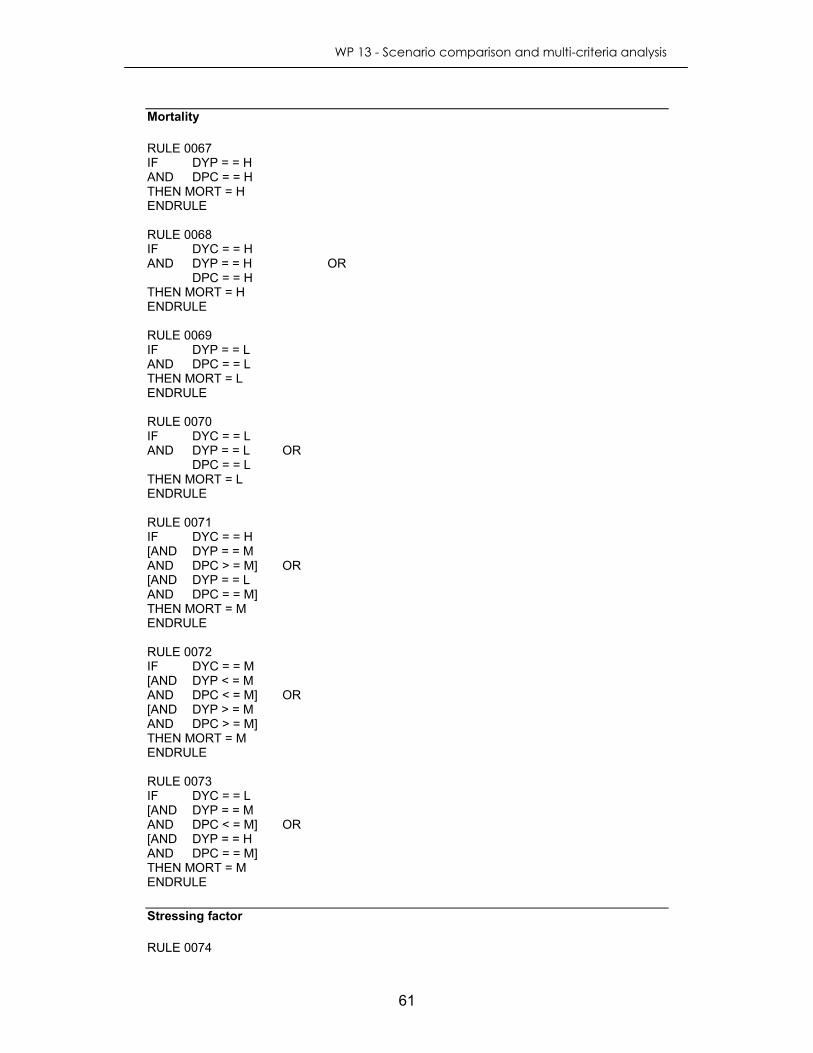
WP 13 - Scenario comparison and multi-criteria analysis
61
Mortality RULE 0067 IF DYP = = H AND DPC = = H THEN MORT = H ENDRULE RULE 0068 IF DYC = = H AND DYP = = H OR DPC = = H THEN MORT = H ENDRULE RULE 0069 IF DYP = = L AND DPC = = L THEN MORT = L ENDRULE RULE 0070 IF DYC = = L AND DYP = = L OR DPC = = L THEN MORT = L ENDRULE RULE 0071 IF DYC = = H [AND DYP = = M AND DPC > = M] OR [AND DYP = = L AND DPC = = M] THEN MORT = M ENDRULE RULE 0072 IF DYC = = M [AND DYP < = M AND DPC < = M] OR [AND DYP > = M AND DPC > = M] THEN MORT = M ENDRULE RULE 0073 IF DYC = = L [AND DYP = = M AND DPC < = M] OR [AND DYP = = H AND DPC = = M] THEN MORT = M ENDRULE Stressing factor RULE 0074
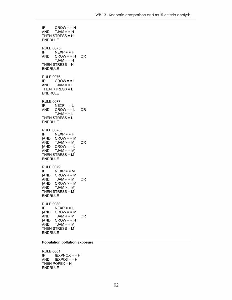
WP 13 - Scenario comparison and multi-criteria analysis
62
IF CROW = = H AND TJAM = = H THEN STRESS = H ENDRULE RULE 0075 IF NEXP = = H AND CROW = = H OR TJAM = = H THEN STRESS = H ENDRULE RULE 0076 IF CROW = = L AND TJAM = = L THEN STRESS = L ENDRULE RULE 0077 IF NEXP = = L AND CROW = = L OR TJAM = = L THEN STRESS = L ENDRULE RULE 0078 IF NEXP = = H [AND CROW = = M AND TJAM > = M] OR [AND CROW = = L AND TJAM = = M] THEN STRESS = M ENDRULE RULE 0079 IF NEXP = = M [AND CROW < = M AND TJAM < = M] OR [AND CROW > = M AND TJAM > = M] THEN STRESS = M ENDRULE RULE 0080 IF NEXP = = L [AND CROW = = M AND TJAM < = M] OR [AND CROW = = H AND TJAM = = M] THEN STRESS = M ENDRULE Population pollution exposure RULE 0081 IF IEXPNOX = = H AND IEXPO3 = = H THEN POPEX = H ENDRULE

WP 13 - Scenario comparison and multi-criteria analysis
63
RULE 0082 IF IEXPPM10 = = H AND IEXPNOX = = H OR IEXPO3 = = H THEN POPEX = H ENDRULE RULE 0083 IF IEXPNOX = = L AND IEXPO3 = = L THEN POPEX = L ENDRULE RULE 0084 IF IEXPPM10 = = L AND IEXPNOX = = L OR IEXPO3 = = L THEN POPEX = L ENDRULE RULE 0085 IF IEXPPM10 = = H [AND IEXPNOX = = M AND IEXPO3 > = M] OR [AND IEXPNOX = = L AND IEXPO3 = = M] THEN POPEX = M ENDRULE RULE 0086 IF IEXPPM10 = = M [AND IEXPNOX < = M AND IEXPO3 < = M] OR [AND IEXPNOX > = M AND IEXPO3 > = M] THEN POPEX = M ENDRULE RULE 0087 IF IEXPPM10 = = L [AND IEXPNOX = = M AND IEXPO3 < = M] OR [AND IEXPNOX = = H AND IEXPO3 = = M] THEN POPEX = M ENDRULE City dynamism RULE 0088 IF PU18 = = H AND PO64 = = L THEN CDYN = H ENDRULE RULE 0089 IF INH = = H AND PU18 = = H OR

WP 13 - Scenario comparison and multi-criteria analysis
64
PO64 = = L THEN CDYN = H ENDRULE RULE 0090 IF PU18 = = L AND PO64 = = H THEN CDYN = L ENDRULE RULE 0091 IF INH = = L AND PU18 = = L OR PO64 = = H THEN CDYN = L ENDRULE RULE 0092 IF INH = = H [AND PU18 = = M AND PO64 > = M] OR [AND PU18 = = L AND PO64 = = M] THEN CDYN = M ENDRULE RULE 0093 IF INH = = M [AND PU18 < = M AND PO64 < = M] OR [AND PU18 > = M AND PO64 > = M] THEN CDYN = M ENDRULE RULE 0094 IF INH = = L [AND PU18 = = M AND PO64 < = M] OR [AND PU18 = = H AND PO64 = = M] THEN CDYN = M ENDRULE Morbidity RULE 0095 IF DAYL > = M AND MPC = = H THEN MORB = H ENDRULE RULE 0096 IF DAYL = = H AND MPC = = M THEN MORB = H ENDRULE RULE 0097 IF DAYL < = M
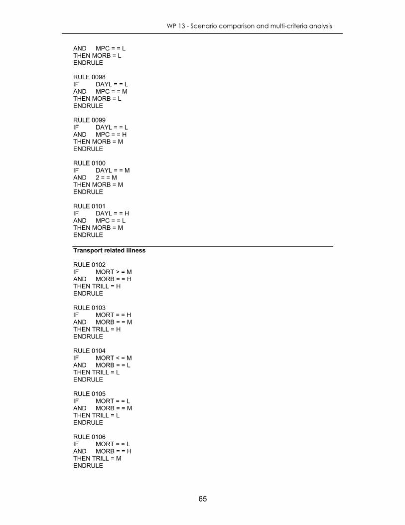
WP 13 - Scenario comparison and multi-criteria analysis
65
AND MPC = = L THEN MORB = L ENDRULE RULE 0098 IF DAYL = = L AND MPC = = M THEN MORB = L ENDRULE RULE 0099 IF DAYL = = L AND MPC = = H THEN MORB = M ENDRULE RULE 0100 IF DAYL = = M AND 2 = = M THEN MORB = M ENDRULE RULE 0101 IF DAYL = = H AND MPC = = L THEN MORB = M ENDRULE Transport related illness RULE 0102 IF MORT > = M AND MORB = = H THEN TRILL = H ENDRULE RULE 0103 IF MORT = = H AND MORB = = M THEN TRILL = H ENDRULE RULE 0104 IF MORT < = M AND MORB = = L THEN TRILL = L ENDRULE RULE 0105 IF MORT = = L AND MORB = = M THEN TRILL = L ENDRULE RULE 0106 IF MORT = = L AND MORB = = H THEN TRILL = M ENDRULE

WP 13 - Scenario comparison and multi-criteria analysis
66
RULE 0107 IF MORT = = M AND 2 = = M THEN TRILL = M ENDRULE RULE 0108 IF MORT = = H AND MORB = = L THEN TRILL = M ENDRULE Transport requirements RULE 0109 IF CDYN > = M AND USPR = = H THEN TREQ = H ENDRULE RULE 0110 IF CDYN = = H AND USPR = = M THEN TREQ = H ENDRULE RULE 0111 IF CDYN < = M AND USPR = = L THEN TREQ = L ENDRULE RULE 0112 IF CDYN = = L AND USPR = = M THEN TREQ = L ENDRULE RULE 0113 IF CDYN = = L AND USPR = = H THEN TREQ = M ENDRULE RULE 0114 IF CDYN = = M AND USPR = = M THEN TREQ = M ENDRULE RULE 0115 IF CDYN = = H AND USPR = = L THEN TREQ = M ENDRULE Transport efficiency RULE 0116 IF NTECHP > = M
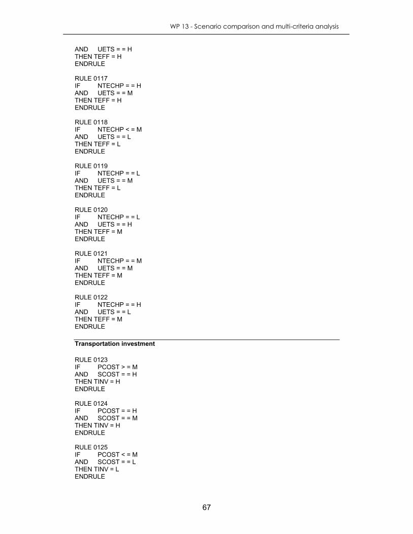
WP 13 - Scenario comparison and multi-criteria analysis
67
AND UETS = = H THEN TEFF = H ENDRULE RULE 0117 IF NTECHP = = H AND UETS = = M THEN TEFF = H ENDRULE RULE 0118 IF NTECHP < = M AND UETS = = L THEN TEFF = L ENDRULE RULE 0119 IF NTECHP = = L AND UETS = = M THEN TEFF = L ENDRULE RULE 0120 IF NTECHP = = L AND UETS = = H THEN TEFF = M ENDRULE RULE 0121 IF NTECHP = = M AND UETS = = M THEN TEFF = M ENDRULE RULE 0122 IF NTECHP = = H AND UETS = = L THEN TEFF = M ENDRULE Transportation investment RULE 0123 IF PCOST > = M AND SCOST = = H THEN TINV = H ENDRULE RULE 0124 IF PCOST = = H AND SCOST = = M THEN TINV = H ENDRULE RULE 0125 IF PCOST < = M AND SCOST = = L THEN TINV = L ENDRULE
WP 13 - Scenario comparison and multi-criteria analysis
68
RULE 0126 IF PCOST = = L AND SCOST = = M THEN TINV = L ENDRULE RULE 0127 IF PCOST = = L AND SCOST = = H THEN TINV = M ENDRULE RULE 0128 IF PCOST = = M AND SCOST = = M THEN TINV = M ENDRULE RULE 0129 IF PCOST = = H AND SCOST = = L THEN TINV = M ENDRULE Transport reliability RULE 0130 IF TTC > = M AND TCPTC = = H THEN TREL = H ENDRULE RULE 0131 IF TTC = = H AND TCPTC = = M THEN TREL = H ENDRULE RULE 0132 IF TTC < = M AND TCPTC = = L THEN TREL = L ENDRULE RULE 0133 IF TTC = = L AND TCPTC = = M THEN TREL = L ENDRULE RULE 0134 IF TTC = = L AND TCPTC = = H THEN TREL = M ENDRULE RULE 0135 IF TTC = = M AND TCPTC = = M
WP 13 - Scenario comparison and multi-criteria analysis
69
THEN TREL = M ENDRULE RULE 0136 IF TTC = = H AND TCPTC = = L THEN TREL = M ENDRULE Atmospheric O3 concentration RULE 0137 IF AAO3 > = M AND IND120O3 = = H THEN O3C = H ENDRULE RULE 0138 IF AAO3 = = H AND IND120O3 = = M THEN O3C = H ENDRULE RULE 0139 IF AAO3 < = M AND IND120O3 = = L THEN O3C = L ENDRULE RULE 0140 IF AAO3 = = L AND IND120O3 = = M THEN O3C = L ENDRULE RULE 0141 IF AAO3 = = L AND IND120O3 = = H THEN O3C = M ENDRULE RULE 0142 IF AAO3 = = M AND 2 = = M THEN O3C = M ENDRULE RULE 0143 IF AAO3 = = H AND IND120O3 = = L THEN O3C = M ENDRULE Living standard RULE 0144 IF PEMS = = H AND PEMT = = H THEN LSTA = H

WP 13 - Scenario comparison and multi-criteria analysis
70
ENDRULE RULE 0145 IF GDP = = H AND PEMS = = H OR PEMT = = H THEN LSTA = H ENDRULE RULE 0146 IF PEMS = = L AND PEMT = = L THEN LSTA = L ENDRULE RULE 0147 IF GDP = = L AND PEMS = = L OR PEMT = = L THEN LSTA = L ENDRULE RULE 0148 IF GDP = = H [AND PEMS = = M AND PEMT < = M] OR [AND PEMS = = L AND PEMT = = M] THEN LSTA = M ENDRULE RULE 0149 IF GDP = = M [AND PEMS < = M AND PEMT > = M] OR [AND PEMS > = M AND PEMT < = M] THEN LSTA = M ENDRULE RULE 0150 IF GDP = = L [AND PEMS = = M AND PEMT > = M] OR [AND PEMS = = H AND PEMT = = M] THEN LSTA = M ENDRULE Primary costs of transportation system RULE 0151 IF ADCC > = M AND ADCP = = H THEN PCOST = H ENDRULE RULE 0152 IF ADCC = = H AND ADCP = = M

WP 13 - Scenario comparison and multi-criteria analysis
71
THEN PCOST = H ENDRULE RULE 0153 IF ADCC < = M AND ADCP = = L THEN PCOST = L ENDRULE RULE 0154 IF ADCC = = L AND ADCP = = M THEN PCOST = L ENDRULE RULE 0155 IF ADCC = = L AND ADCP = = H THEN PCOST = M ENDRULE RULE 0156 IF ADCC = = M AND ADCP = = M THEN PCOST = M ENDRULE RULE 0157 IF ADCC = = H AND ADCP = = L THEN PCOST = M ENDRULE Secondary costs of transportation system RULE 0158 IF ADC > = M AND ADP = = H THEN SCOST = H ENDRULE RULE 0159 IF ADC = = H AND ADP = = M THEN SCOST = H ENDRULE RULE 0160 IF ADC < = M AND ADP = = L THEN SCOST = L ENDRULE RULE 0161 IF ADC = = L AND ADP = = M THEN SCOST = L ENDRULE RULE 0162

WP 13 - Scenario comparison and multi-criteria analysis
72
IF ADC = = L AND ADP = = H THEN SCOST = M ENDRULE RULE 0163 IF ADC = = M AND ADP = = M THEN SCOST = M ENDRULE RULE 0164 IF ADC = = H AND ADP = = L THEN SCOST = M ENDRULE Economical transport performance RULE 0165 IF TEFF = = H AND 2 = = H [AND LSTA > = M AND TREL = = H] OR [AND LSTA = = H AND TREL > = M] THEN ECOTP = EX ENDRULE RULE 0166 IF LSTA = = H AND TREL = = H [AND TEFF = = M AND 2 = = H] OR [AND TEFF = = H AND 2 = = M] THEN ECOTP = EX ENDRULE RULE 0167 IF TEFF = = H AND TINV = = H [AND LSTA = = L AND TREL > = M] OR [AND LSTA < = M AND TREL = M] OR [AND LSTA > = M AND TREL = = L] THEN ECOTP = G ENDRULE RULE 0168 IF TEFF = = M AND TINV = = H [AND LSTA < = M AND TREL = H] OR [AND LSTA > = M AND TREL = = M] OR [AND LSTA = = H AND TREL = = L]

WP 13 - Scenario comparison and multi-criteria analysis
73
THEN ECOTP = G ENDRULE RULE 0169 IF TEFF = = H AND TINV = = M [AND LSTA < = M AND TREL = H] OR [AND LSTA > = M AND TREL = = M] OR [AND LSTA = = H AND TREL = = L] THEN ECOTP = G ENDRULE RULE 0170 IF TEFF = = L AND TINV = = H [AND LSTA > = M AND TREL = = H] OR [AND LSTA = = H AND TREL = = M] THEN ECOTP = G ENDRULE RULE 0171 IF TEFF = = M AND TINV = = M [AND LSTA > = M AND TREL = = H] OR [AND LSTA = = H AND TREL = = M] THEN ECOTP = G ENDRULE RULE 0172 IF TEFF = = H AND TINV = = L [AND LSTA > = M AND TREL = = H] OR [AND LSTA = = H AND TREL = = M] THEN ECOTP = G ENDRULE RULE 0173 IF LSTA = = H AND TREL = = H [AND TEFF = = L AND TINV = = M] OR [AND TEFF = = M AND TINV = = L] THEN ECOTP = G ENDRULE RULE 0174 IF TEFF = = H AND TINV = = H AND LSTA = = L AND TREL = = L
WP 13 - Scenario comparison and multi-criteria analysis
74
THEN ECOTP = A ENDRULE RULE 0175 IF TEFF = = M AND TINV = = H [AND LSTA = = L AND TREL = = M] OR [AND LSTA = = M AND TREL = = L] THEN ECOTP = A ENDRULE RULE 0176 IF TEFF = = H AND TINV = = M [AND LSTA = = L AND TREL = = M] OR [AND LSTA = = M AND TREL = = L] THEN ECOTP = A ENDRULE RULE 0177 IF TEFF = = L AND TINV = = H [AND LSTA = = L AND TREL = = M] OR [AND LSTA = = M AND TREL = = L] THEN ECOTP = A ENDRULE RULE 0178 IF TEFF = = M AND TINV = = M [AND LSTA = = L AND TREL = = M] OR [AND LSTA = = M AND TREL = = L] THEN ECOTP = A ENDRULE RULE 0179 IF TEFF = = H AND TINV = = L [AND LSTA = = L AND TREL = = M] OR [AND LSTA = = M AND TREL = = L] THEN ECOTP = A ENDRULE RULE 0180 IF TEFF = = L AND TINV = = M [AND LSTA = = M AND TREL = = H] OR [AND LSTA = = H AND TREL = = M]

WP 13 - Scenario comparison and multi-criteria analysis
75
THEN ECOTP = A ENDRULE RULE 0181 IF TEFF = = M AND TINV = = L [AND LSTA = = M AND TREL = = H] OR [AND LSTA = = H AND TREL = = M] THEN ECOTP = A ENDRULE RULE 0182 IF TEFF = = L AND TINV = = L AND LSTA = = H AND TREL = = H THEN ECOTP = A ENDRULE RULE 0183 IF LSTA = = L AND TREL = = L [AND TEFF = = M AND TINV = = H] OR [AND TEFF = = H AND TINV = = M] THEN ECOTP = P ENDRULE RULE 0184 IF LSTA = L AND TREL < = M [AND TEFF = = L AND TINV = = H] OR [AND TEFF = = M AND TINV = = M] OR [AND TEFF = = H AND TINV = = L] THEN ECOTP = P ENDRULE RULE 0185 IF LSTA = M AND TREL = = L [AND TEFF = = L AND TINV = = H] OR [AND TEFF = = M AND TINV = = M] OR [AND TEFF = = H AND TINV = = L] THEN ECOTP = P ENDRULE RULE 0186 IF TEFF = = L AND TINV = = M [AND LSTA = = L AND TREL > = M] OR

WP 13 - Scenario comparison and multi-criteria analysis
76
[AND LSTA = = M AND TREL < = M] OR [AND LSTA = = H AND TREL = = L] THEN ECOTP = P ENDRULE RULE 0187 IF TEFF = = M AND TINV = = L [AND LSTA = = L AND TREL > = M] OR [AND LSTA = = M AND TREL < = M] OR [AND LSTA = = H AND TREL = = L] THEN ECOTP = P ENDRULE RULE 0188 IF TEFF = = L AND TINV = = L [AND LSTA < = M AND TREL = = H] OR [AND LSTA > = M AND TREL = = M] OR [AND LSTA = = H AND TREL = = L] THEN ECOTP = P ENDRULE RULE 0189 IF LSTA = = L AND TREL = = L [AND TEFF = = L AND TINV < = M] OR [AND TEFF = = M AND TINV = = L] THEN ECOTP = VP ENDRULE RULE 0190 IF TEFF = = L AND TINV = = L [AND LSTA = = L AND TREL = = M] OR [AND LSTA = = M AND TREL = = L] THEN ECOTP = VP ENDRULE Social transportation impacts RULE 0191 IF HRISK = = H AND TREQ = = H [AND TINT > = M AND TDAN = = H] OR [AND TINT = = H AND TDAN > = M]

WP 13 - Scenario comparison and multi-criteria analysis
77
THEN STP = VP ENDRULE RULE 0192 IF TINT = = H AND TDAN = = H [AND HRISK = = M AND TREQ = = H] OR [AND HRISK = = H AND TREQ = = M] THEN STP = VP ENDRULE RULE 0193 IF HRISK = = H AND TREQ = = H [AND TINT = = L AND TDAN > = M] OR [AND TINT < = M AND TDAN = M] OR [AND TINT > = M AND TDAN = = L] THEN STP = P ENDRULE RULE 0194 IF HRISK = = M AND TREQ = = H [AND TINT < = M AND TDAN = H] OR [AND TINT > = M AND TDAN = = M] OR [AND TINT = = H AND TDAN = = L] THEN STP = P ENDRULE RULE 0195 IF HRISK = = H AND TREQ = = M [AND TINT < = M AND TDAN = H] OR [AND TINT > = M AND TDAN = = M] OR [AND TINT = = H AND TDAN = = L] THEN STP = P ENDRULE RULE 0196 IF HRISK = = L AND TREQ = = H [AND TINT > = M AND TDAN = = H] OR [AND TINT = = H AND TDAN = = M] THEN STP = P ENDRULE RULE 0197
WP 13 - Scenario comparison and multi-criteria analysis
78
IF HRISK = = M AND TREQ = = M [AND TINT > = M AND TDAN = = H] OR [AND TINT = = H AND TDAN = = M] THEN STP = P ENDRULE RULE 0198 IF HRISK = = H AND TREQ = = L [AND TINT > = M AND TDAN = = H] OR [AND TINT = = H AND TDAN = = M] THEN STP = P ENDRULE RULE 0199 IF TINT = = H AND TDAN = = H [AND HRISK = = L AND TREQ = = M] OR [AND HRISK = = M AND TREQ = = L] THEN STP = P ENDRULE RULE 0200 IF HRISK = = H AND TREQ = = H AND TINT = = L AND TDAN = = L THEN STP = A ENDRULE RULE 0201 IF HRISK = = M AND TREQ = = H [AND TINT = = L AND TDAN = = M] OR [AND TINT = = M AND TDAN = = L] THEN STP = A ENDRULE RULE 0202 IF HRISK = = H AND TREQ = = M [AND TINT = = L AND TDAN = = M] OR [AND TINT = = M AND TDAN = = L] THEN STP = A ENDRULE RULE 0203 IF HRISK = = L AND TREQ = = H
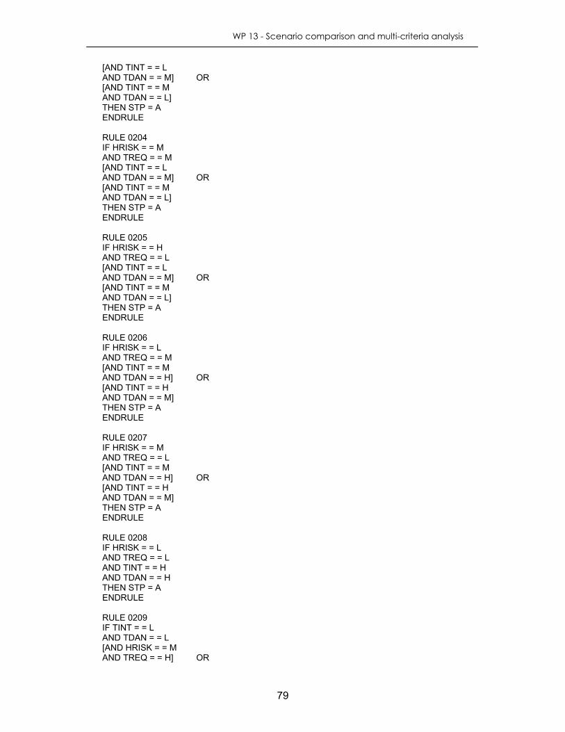
WP 13 - Scenario comparison and multi-criteria analysis
79
[AND TINT = = L AND TDAN = = M] OR [AND TINT = = M AND TDAN = = L] THEN STP = A ENDRULE RULE 0204 IF HRISK = = M AND TREQ = = M [AND TINT = = L AND TDAN = = M] OR [AND TINT = = M AND TDAN = = L] THEN STP = A ENDRULE RULE 0205 IF HRISK = = H AND TREQ = = L [AND TINT = = L AND TDAN = = M] OR [AND TINT = = M AND TDAN = = L] THEN STP = A ENDRULE RULE 0206 IF HRISK = = L AND TREQ = = M [AND TINT = = M AND TDAN = = H] OR [AND TINT = = H AND TDAN = = M] THEN STP = A ENDRULE RULE 0207 IF HRISK = = M AND TREQ = = L [AND TINT = = M AND TDAN = = H] OR [AND TINT = = H AND TDAN = = M] THEN STP = A ENDRULE RULE 0208 IF HRISK = = L AND TREQ = = L AND TINT = = H AND TDAN = = H THEN STP = A ENDRULE RULE 0209 IF TINT = = L AND TDAN = = L [AND HRISK = = M AND TREQ = = H] OR

WP 13 - Scenario comparison and multi-criteria analysis
80
[AND HRISK = = H AND TREQ = = M] THEN STP = G ENDRULE RULE 0210 IF TINT = L AND TDAN < = M [AND HRISK = = L AND TREQ = = H] OR [AND HRISK = = M AND TREQ = = M] OR [AND HRISK = = H AND TREQ = = L] THEN STP = G ENDRULE RULE 0211 IF TINT = M AND TDAN = = L [AND HRISK = = L AND TREQ = = H] OR [AND HRISK = = M AND TREQ = = M] OR [AND HRISK = = H AND TREQ = = L] THEN STP = G ENDRULE RULE 0212 IF HRISK = = L AND TREQ = = M [AND TINT = = L AND TDAN > = M] OR [AND TINT = = M AND TDAN < = M] OR [AND TINT = = H AND TDAN = = L] THEN STP = G ENDRULE RULE 0213 IF HRISK = = M AND TREQ = = L [AND TINT = = L AND TDAN > = M] OR [AND TINT = = M AND TDAN < = M] OR [AND TINT = = H AND TDAN = = L] THEN STP = G ENDRULE RULE 0214 IF HRISK = = L AND TREQ = = L [AND TINT < = M AND TDAN = = H] OR [AND TINT > = M AND TDAN = = M] OR

WP 13 - Scenario comparison and multi-criteria analysis
81
[AND TINT = = H AND TDAN = = L] THEN STP = G ENDRULE RULE 0215 IF TINT = = L AND TDAN = = L [AND HRISK = = L AND TREQ < = M] OR [AND HRISK = = M AND TREQ = = L] THEN STP = EX ENDRULE RULE 0216 IF HRISK = = L AND TREQ = = L [AND TINT = = L AND TDAN = = M] OR [AND TINT = = M AND TDAN = = L] THEN STP = EX ENDRULE Air quality RULE 0217 IF NOXC > = M AND O3C = = H THEN AQ = H ENDRULE RULE 0218 IF NOXC = = H AND O3C = = M THEN AQ = H ENDRULE RULE 0219 IF NOXC < = M AND O3C = = L THEN AQ = L ENDRULE RULE 0220 IF NOXC = = L AND O3C = = M THEN AQ = L ENDRULE RULE 0221 IF NOXC = = L AND O3C = = H THEN AQ = M ENDRULE RULE 0222 IF NOXC = = M AND O3C = = M

WP 13 - Scenario comparison and multi-criteria analysis
82
THEN AQ = M ENDRULE RULE 0223 IF NOXC = = H AND O3C = = L THEN AQ = M ENDRULE ENVIRONMENTAL QUALITY RULE 0224 IF EPRES = = H [AND AQ < = M AND FFC = = H] OR [AND AQ = = L AND FFC = = M] THEN ENVQ = EX ENDRULE RULE 0225 IF EPRES = = M AND AQ = = L AND FFC = = H THEN ENVQ = EX ENDRULE RULE 0226 IF EPRES = = H [AND AQ = = H AND FFC = = H] OR [AND AQ = = M AND FFC = = M] OR [AND AQ = = L AND FFC = =L] THEN ENVQ = G ENDRULE RULE 0227 IF EPRES = = M [AND AQ = = M AND FFC = = H] OR [AND AQ = = L AND FFC = = M] THEN ENVQ = G ENDRULE RULE 0228 IF EPRES = = L AND AQ = = L AND FFC = = H THEN ENVQ = G ENDRULE RULE 0229 IF EPRES = = H [AND AQ = = H AND FFC = = M] OR [AND AQ = = M AND FFC = = L]

WP 13 - Scenario comparison and multi-criteria analysis
83
THEN ENVQ = A ENDRULE RULE 0230 IF EPRES = = M [AND AQ = = H AND FFC = = H] OR [AND AQ = = M AND FFC = = M] OR [AND AQ = = L AND FFC = =L] THEN ENVQ = A ENDRULE RULE 0231 IF EPRES = = L [AND AQ = = M AND FFC = = H] OR [AND AQ = = L AND FFC = = M] THEN ENVQ = A ENDRULE RULE 0232 IF EPRES = = H AND AQ = = H AND FFC = = L THEN ENVQ = P ENDRULE RULE 0233 IF EPRES = = M [AND AQ = = H AND FFC = = M] OR [AND AQ = = M AND FFC = = L] THEN ENVQ = P ENDRULE RULE 0234 IF EPRES = = L [AND AQ = = H AND FFC = = H] OR [AND AQ = = M AND FFC = = M] OR [AND AQ = = L AND FFC = =L] THEN ENVQ = P ENDRULE RULE 0235 IF EPRES = = M AND AQ = = H AND FFC = = L THEN ENVQ = VP ENDRULE RULE 0236 IF EPRES = = L [AND AQ > = M

WP 13 - Scenario comparison and multi-criteria analysis
84
AND FFC = = L] OR [AND AQ = = H AND FFC = = M] THEN ENVQ = VP ENDRULE SUSTAINABLE TRANSPORT PERFORMANCE RULE 0237 IF ENVQ = = EX [AND SOCTP > = G AND ECOTP = = EX] OR [AND SOCTP = = EX AND ECOTP = = G] THEN SUSTP = EX ENDRULE RULE 0238 IF ENVQ = = G AND SOCTP = = EX AND ECOTP = = EX THEN SUSTP = EX ENDRULE RULE 0239 IF ENVQ = = EX [AND SOCTP < = A AND ECOTP = = EX] OR [AND SOCTP < = G AND SOCTP > = P AND ECOTP = = G] OR [AND SOCTP > = A AND ECOTP = = A] OR [AND SOCTP > = G AND ECOTP = = P] OR [AND SOCTP = = EX AND ECOTP = = VP] THEN SUSTP = G ENDRULE RULE 0240 IF ENVQ = = EX [AND SOCTP = = VP AND ECOTP = = G] OR [AND SOCTP < = P AND ECOTP = = A] OR [AND SOCTP < = A AND ECOTP = = P] OR [AND SOCTP < = G AND SOCTP > = P AND ECOTP = = VP] THEN SUSTP = A ENDRULE RULE 0241 IF ENVQ = = EX AND SOCTP = = VP AND ECOTP = = VP THEN SUSTP = P

WP 13 - Scenario comparison and multi-criteria analysis
85
ENDRULE RULE 0242 IF ENVQ = = P [AND SOCTP > = G AND ECOTP = = EX] OR [AND SOCTP = = EX AND ECOTP = = G] THEN SUSTP = G ENDRULE RULE 0243 IF ENVQ = = P AND SOCTP = = EX AND ECOTP = = EX THEN SUSTP = G ENDRULE RULE 0244 IF ENVQ = = P [AND SOCTP < = A AND ECOTP = = EX] OR [AND SOCTP < = G AND SOCTP > = P AND ECOTP = = G] OR [AND SOCTP > = A AND ECOTP = = A] OR [AND SOCTP > = G AND ECOTP = = P] OR [AND SOCTP = = EX AND ECOTP = = VP] THEN SUSTP = A ENDRULE RULE 0245 IF ENVQ = = P [AND SOCTP = = VP AND ECOTP = = G] OR [AND SOCTP < = P AND ECOTP = = A] OR [AND SOCTP < = A AND ECOTP = = P] OR [AND SOCTP < = G AND SOCTP > = P AND ECOTP = = VP] THEN SUSTP = P ENDRULE RULE 0246 IF ENVQ = = P AND SOCTP = = VP AND ECOTP = = VP THEN SUSTP = VP ENDRULE RULE 0247 IF ENVQ = = G AND SOCTP = = EX AND ECOTP = = EX THEN SUSTP = = EX

WP 13 - Scenario comparison and multi-criteria analysis
86
ENDRULE RULE 0248 IF ENVQ = = G [AND SOCTP < = G AND SOCTP > = P AND ECOTP = = EX] OR [AND SOCTP > = A AND ECOTP = = G] OR [AND SOCTP > = G AND ECOTP = = A] OR [AND SOCTP = = EX AND ECOTP = = P] THEN SUSTP = G ENDRULE RULE 0249 IF ENVQ = = G [AND SOCTP = = VP AND ECOTP = = EX] OR [AND SOCTP < = P AND ECOTP = = G] OR [AND SOCTP < = A AND ECOTP = = A] OR [AND SOCTP < = G AND SOCTP > = P AND ECOTP = = P] OR [AND SOCTP > = A AND ECOTP = = VP] THEN SUSTP = A ENDRULE RULE 0250 IF ENVQ = = G [AND SOCTP < = P AND ECOTP = = VP] OR [AND SOCTP = = VP AND ECOTP = = P] THEN SUSTP = P ENDRULE RULE 0251 IF ENVQ = = VP AND SOCTP = = EX AND ECOTP = = EX THEN SUSTP = = G ENDRULE RULE 0252 IF ENVQ = = VP [AND SOCTP < = G AND SOCTP > = P AND ECOTP = = EX] OR [AND SOCTP > = A AND ECOTP = = G] OR [AND SOCTP > = G AND ECOTP = = A] OR [AND SOCTP = = EX AND ECOTP = = P] THEN SUSTP = A

WP 13 - Scenario comparison and multi-criteria analysis
87
ENDRULE RULE 0253 IF ENVQ = = VP [AND SOCTP = = VP AND ECOTP = = EX] OR [AND SOCTP < = P AND ECOTP = = G] OR [AND SOCTP < = A AND ECOTP = = A] OR [AND SOCTP < = G AND SOCTP > = P AND ECOTP = = P] OR [AND SOCTP > = A AND ECOTP = = VP] THEN SUSTP = P ENDRULE RULE 0254 IF ENVQ = = VP [AND SOCTP < = P AND ECOTP = = VP] OR [AND SOCTP = = VP AND ECOTP = = P] THEN SUSTP = VP ENDRULE RULE 0255 IF ENVQ = = A [AND SOCTP > = A AND ECOTP = = EX] OR [AND SOCTP > = G AND ECOTP = = G] OR [AND SOCTP = = EX AND ECOTP = = A] THEN SUSTP = G ENDRULE RULE 0256 IF ENVQ = = A [AND SOCTP < = P AND ECOTP = = EX] OR [AND SOCTP < = A AND ECOTP = = G] OR [AND SOCTP < = G AND SOCTP > = A AND ECOTP = = A] OR [AND SOCTP > = A AND ECOTP = = P] OR [AND SOCTP > = G AND ECOTP = = VP] THEN SUSTP = A ENDRULE RULE 0257 IF ENVQ = = A [AND SOCTP = = VP AND ECOTP = = A] OR [AND SOCTP < = P AND ECOTP = = P] OR

WP 13 - Scenario comparison and multi-criteria analysis
88
[AND SOCTP < = A AND ECOTP = = VP] THEN SUSTP = P ENDRULE

WP 13 - Scenario comparison and multi-criteria analysis
89
9. REFERENCES Cellura, Beccali etal: “A decision support system software based on Multi-Criteria Analysis for the Selection of Urban Sustainability Scenarios” Palerno University, Italy 2002 DTLR Multi-criteria analysis: a manual: http://www.dtlr.gov.uk/about/multicriteria/ Fedra, K., Winkelbauer, L. “Expert Systems for Environmental Screening – An application in the Lower Mekong Basin” International Institute for Applied System Analysis, 1991. Fet, Michelsen, Johnsen: “Environmental Performance of Transportation – A comparative Study” 2000 Valentin, Spangenberg: “Indicators for Sustainable Communities” 1999 Kuenzli, N., Kaiser, R., “Public-health impact of outdoor and traffic-related air pollution: a European assessment” The Lancet, Vol. 356, September 2000. Litman T & Burwell D: “Issues in Sustainable Transportation” Victoria Transport Policy Institute 2003 Litman T: “Sustainable Transportation Indicators” Victoria Transport Policy Institute 2003 The Regional Environmental Center for Central and Eastern Europe website http://www.rec.org/ “Environmentally Sustainable Transportation Indicators – A discussion paper” European Sustainable Cities website http://europa.eu.int/comm/environment/urban/home_en.htm Expert Systems: http://www.cee.hw.ac.uk/~alison/ai3notes/chapter2_5.html Engelmore, R.S., Feigenbaum, E., Expert Systems and Artificial Intelligence http://www.wtec.org/loyola/kb/c1_s1.htm