raymond t. pierrehumbert the university of chicago · r-c modeling, exoclimes 2011...

R-C Modeling, Exoclimes 2011

Radiative-Convective Modeling of Planetary Climate

Raymond T. Pierrehumbert

The University of Chicago

1


Outline of the Lecture

• Basic formulation and solution methods

• Some interesting applications

• Beyond 1D: The need for dynamics

2


Basic formulation: What is a radiative convective model?

• Represent entire atmosphere by a single vertical column T (p, t), etc.

• Column generally meant to represent global mean climate

• Only vertical energy transport is modeled

– Radiative transport

– Turbulent transport due to convection

– Convection modeled as a 1D mixing process

3


For further reading ...

4


Radiating temperature and the greenhouse effect

Tg

T(ps)

Radiation only

TemperatureRadiation

and Turbulence

For many purposes, can assume Tg ≈ T (ps)

For review, see: Pierrehumbert 2010: Infrared Radiation and PlanetaryTemperature, Physics Today 64

5

Abisko 2011: Energy Balance and Planetary Temperature

A few observed vertical structures

10

100

1000

150 180 210 240 270 300

March 15 1993, 12Z2.00 S 169.02 W

Pres

sure

(m

illib

ars)

Temperature (Kelvin)

Tropopause

Troposphere

Stratosphere

100 200 300 400 500 600 700 800

0.001

0.01

0.1

1

10

100

Venus

Pioneer Venus Large Probe, 1978Magellan Radio 1990

T

p (b

ars)

60 80 100 120 140 160 180

1

10

100

1000

Titan (Huygens Data)

T

p (m

illib

ars)

100 150 200 250 300 350 400 450

10-5

0.0001

0.001

0.01

0.1

1

10

Jupiter

T

p (b

ars)

6


The IR Radiative Transfer model

• Input T (p), composition (e.g. pCO2,q(p))

• → fluxes I+(p), I−(p)

• Heating rate H = g−1d(I+ − I−)/dp

7


Pure radiative equilibrium

• H + Hsw = 0 at each p

• Equivalently I+ − I−+ F~ = const.

• Typically ignore scattering for IR, but incorporate it for F~

• Wavelength of incoming stellar radiation�Wavelength of outgoing IR

• ... but this separation can break down for roasters.

8


Energy balance for atmosphere transparent to incoming stellarradiation

120 160 200 240 280

2 104

4 104

6 104

8 104

1 105

Radiative-ConvectiveDry AdiabatPure Radiative Equilibrium

T (K)

pres

sure

(Pa)

300ppmv CO2

in Dry Air

Tropopause

-0.004 -0.002 0 0.002

2 104

4 104

6 104

8 104

1 105

Radiative-ConvectiveDry Adiabat

IR Heating Rate (W/kg)

pres

sure

(Pa)

300ppmv CO2

in Dry Air

Warm A

ir Up

Warm A

ir Up

Cold Air Down

Cold Air Down

(∫ pspt

Hdp/g) + Sabs = 0 ; Determines tropopause height

9


How to get OLR(Tg)

Time steppingrequired here

IR

OLR

Require zeronet flux

No time steppingin troposphere

StratosphereTroposphere

Tg

ptrop

SW

SW

• Without atmospheric shortwave absorption, stratospheric temperaturedepends on insolation only via Tg.

10

• For typical atmospheres stratosphere is optically thin in IR. Can thenuse isothermal stratosphere or ”all troposphere model” and dispensewith time-stepping entirely.


Once you have OLR(Tg) ...

T

OLR

Stellar AbsFlu

x

Plot it, and you’re done!

11


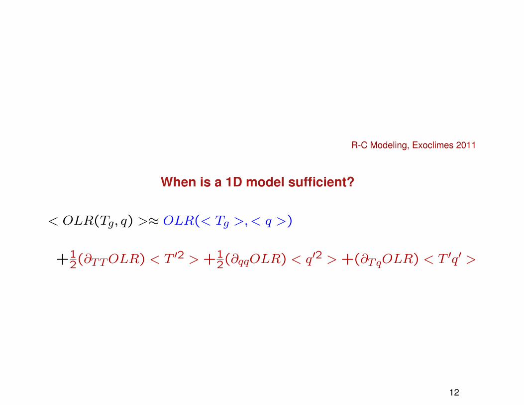
When is a 1D model sufficient?

< OLR(Tg, q) >≈ OLR(< Tg >, < q >)

+12(∂TTOLR) < T ′2 > +1

2(∂qqOLR) < q′2 > +(∂TqOLR) < T ′q′ >

12


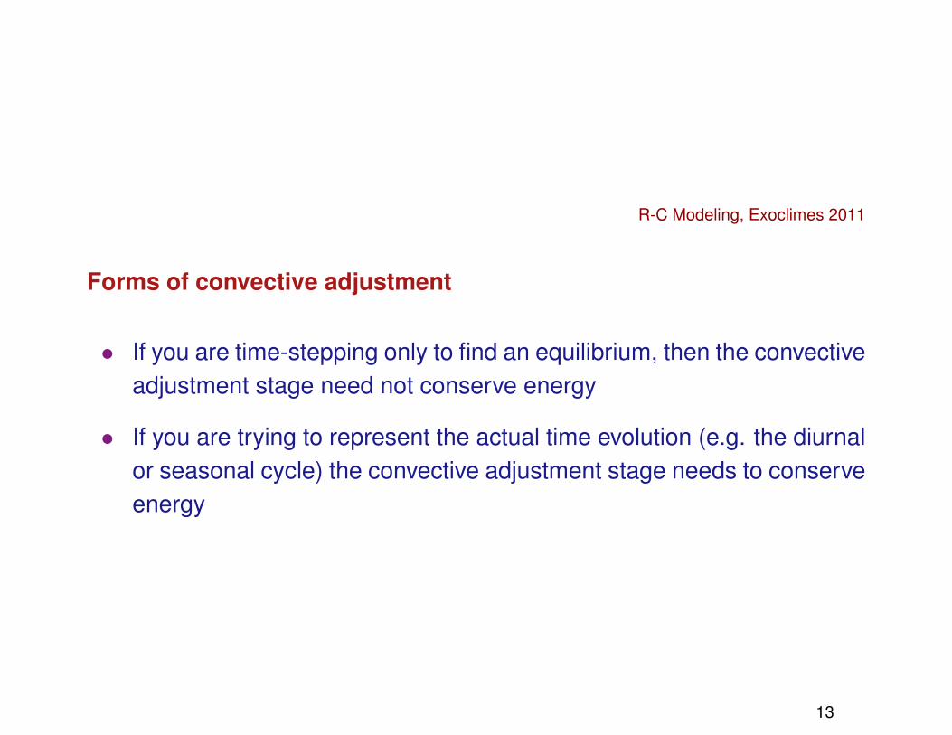
Forms of convective adjustment

• If you are time-stepping only to find an equilibrium, then the convectiveadjustment stage need not conserve energy

• If you are trying to represent the actual time evolution (e.g. the diurnalor seasonal cycle) the convective adjustment stage needs to conserveenergy

13


What is conserved during convective adjustment?

• Suppose the adjustment takes place in a layer from p1 to p2

• The final state is an adiabat. Which adiabat? (e.g. dry adiabat is aone-parameter family defined by T (p) = T (p1)(p/p1)

R/cp)

• First Law: T−1δQ = ds = dcp ln θ

• But during adjustment, δQ 6= 0 at each p. Only have∫ p2p1

δQdp = 0

• Therefore∫ p2p1

T−1δQdp 6= 0; Entropy does not ”mix”

14


The answer: Dry or Moist Static Energy

• Define Z(p) from hydrostatic relation

• First law: δQ = d(cpT + gZ) (in dry case)

• Therefore DSE ≡∫ p2p1

(cpT + gZ)dp/g conserved during adjustment

• If q is the mass concentration of the condensible, then in dilute limit(q � 1), MSE density is cpT + gZ + Lq

• Things get interesting (and somewhat unexplored) in the non-dilutelimit, where you need to track the energy carried by the condensate.

15


Example: DSE-conserving mixing of a step discontinuity

180 200 220 240 260 280 300 320

20000

40000

60000

80000

100000

Tinit

Tadj

Temperature (K)

Pres

sure

(Pa)

1.4 1051.6 1051.8 105 2 105 2.2 1052.4 1052.6 105

20000

40000

60000

80000

100000

DSEinit

DSEadj

Dry Static Energy (J/Kg)

Pres

sure

(Pa)

Unique adjusted solution for any p1 and p2. Adjust p1 and p2 to make thetemperature continuous at endpoints. (An assumption about how

convection works!)16


Deep atmospheres, optically thick in stellar spectrum

ShortwaveAbsorption layer

No net flux in deep layer → isothermal

17


Applications: The conventional habitable zone

• Inner edge: Water vapor runaway (”wet” or ”dry” version).(Runaway = Uninhabitable)

• Outer edge: CO2 runaway.(Runaway = Habitable)

18


Water Vapor runaway and inner edge (pure WV atmosphere)

220

240

260

280

300

320

340

360

380

260 280 300 320 340 360 380 400

100 m/s**2, pure water20 m/s**2, pure water10 m/s**2, pure water1 m/s**2, pure water

OLR

(W

/m2 )

Tg

Abs. solar, g = 20 m/s**2 (schematic)

More on this from Colin!19


CO2 runaway and outer edge edge (pure CO2 atmosphere)

0

20

40

60

80

100

120 140 160 180 200 220 240 260

OLR

(W

/m2 )

Surface Temperature (K)

100 m/s2

20 m/s2

10 m/s2

1 m/s23 m/s2

0.01 0.1 1 10 30Surface Pressure (bar)

Abs. solar, g = 20 m/s**2 (schematic)

Ch. 4, Principles ... plus in-prep radiation model intercomparison byPierrehumbert, Abbot and Halevy

20

Abisko 2011: Energy Balance and Planetary Temperature

Outer edge: Ice-albedo bifurcation

0

100

200

300

400

500

600

700

800

200 220 240 260 280 300 320 340

OLRL=1517L=1685L=1854L=2865

Flux

(W

/m2 )

Surface Temperature

H

Sn1

Ice covered Ice Free

Sn2

Sn3

AB

A'

B'

1

4(1− α(T ))L~ = OLR(T,CO2)

21

Snowbird 2011: Climate sensitivity, feedback and bifurcation

Snowball Earths

Pierrehumbert , Ap. J. L. 2011

Pierrehumbert , Abbot, Voigt & Koll, Ann. Rev. Earth and Plan. Sci. 2011

22

Snowbird 2011: Climate sensitivity, feedback and bifurcation

Zero-D Snowball Bifurcation

1 10 100 1000 104 105220

240

260

280

300

320

340

Glo

bal M

ean

Tem

pera

ture

(K)

55% 60% 65%

L

R

CO2 Inventory (Pa)

CO2 Concentration

S1

S2

S3

S4

W1

W2

W3

W4

.000066.0000066 .00066 .0065 .062 .397

Pierrehumbert,Abbot,Voigt & Koll, AREPS 2011

23


Applications: H2 worlds

• Conventional outer limit defined by CO2 runaway. Yields Early Marsequivalent orbit

• To make planets in more distant orbits habitable you need a less con-densible greenhouse gas

• So how about H2?

• In a distant orbit, a Super-Earth can hold an H2 atmosphere.

• Gravitational lensing has detected Super-Earths in distant orbits.

• Pierrehumbert and Gaidos, ApJL 2011

• Also relevant to Steppenwolf planets

24


Pure H2 atmosphere

0 50 100 150 200 250 300

0.001

0.01

0.1

1

10

Temperature Profiles, Absorbed Stellar Radiation 5 W/m2

AdiabatT (M star)

T (G star)

Temperature (K)

Pres

sure

(bar

)

25


Top-of-Atmosphere Energy Balance

1

10

100

1000

1 10

Flux

per

uni

t sur

face

are

a (W

/m2 )

Surface pressure (bar)

280K300K

320K340K

360K

L = 40 W/m2L = 80 W/m2

26


Beyond 1D: The role of large scale dynamics

• Horizontal heat transport

• Lapse rate

• Subsaturation (Relative Humidity)

• Clouds

27


Intro to General Circulation: The Hadley Cell

90S 60S 30S 0 90N30N 60N1000

800

600

400

200

100

July

Excess EnergyOut

Excess EnergyOut

Excess Energy In

90S 60S 30S 0 90N30N 60N1000

800

600

400

200

100

Excess EnergyOut

Excess EnergyOut

Excess Energy In

January

Gets more global for slow rotation, small planet (Venus,Titan); moreequatorially confined for rapid rotation, large planet (Jupiter, Saturn).

Earth is ”Mr. In-Between.”28


Intro to General Circulation: Extratropical synoptic eddies

Transport hot air poleward/upward, cold air equatorward/downward.

29


Beyond 1D: Lapse Rate

• Hadley cell sets the entire tropics to the moist adiabat, even thoughconvection is active in only a small proportion of the tropics

• In midlatitudes, there may be little convection, and lapse rate is deter-mined by large scale transports of heat by transient baroclinic eddies.Lapse rate can have large geographic and seasonal variation.

30


Example: Siberian lapse rate

200 220 240 260 280 300

200

300

400

500

600

700

800900

1000

Temperature (K)

Pres

sure

(m

b)

55N Asian Continental Interior

Synoptic eddies increase winter stability by sliding in cold polar air at lowaltitudes

31


Beyond 1D: Subsaturation

• Atmospheres with a condensible component need not be saturated

• Subsaturation determines concentration of the condensible (e.g. watervapor)

• Subsaturation is a dynamical phenomenon

• Subsaturation affects runaway at both the inner and outer edge of theHZ.

32


Where does subsaturation come from?

T2<T1

T1 , q1

q2<q1

T3>T1

q3=q2<q1

Saturated Subsaturated

Lift

and

cool Subside and heat

33


Rapid subsidence creates large T (and hence p) gradients

100 200 300 400 500 600 700 800

10000

100000

Temperature (K)

Pres

sure

(Pa)

Subsidence from 10000 Pa to surface

Moist A

scentDry Descent

Radiative Cooling

”Rapid” = ”Rapid compared to radiative cooling”

34


RH feedback leads to metastable non-runaway states

240

260

280

300

320

340

280 300 320 340 360 380 400

RHmin = 25%RHmin = 50%RHmin = 75%RHmin = 100%

OLR

(W/m

2 )

Surface temperature (K)

N2/H

2O Atmosphere

RH = RHmin + (100%−RHmin)(T − T0)/(T1 − T0)

for T0 < T < T1

35


Subsaturation in FMS GCM dynamic simulations

• 3D dynamic general circulation model

• Tide-locked, various orbital periods

• Idealized moist thermodynamics (includes latent heat release)

• Grey gas radiation; no effect of condensible on IR optical depth

• Carried out by Feng Ding

36


Long period orbit

37


Short period orbit

38


A few take-home points

• Radiative-Convective modeling is still a valuable tool.

• Ideal for exploratory work on new problems, testing convection andradiation schemes, etc.

• Energy-conserving convective adjustment for atmospheres with con-densation of a major constituent still has some wrinkles to be workedout.

• Even for planets with quite uniform surface temperature, dynamics hasimportant zero-order climate effects via lapse rate, subsaturation andclouds.

39

raymond t. pierrehumbert the university of chicago · r-c modeling, exoclimes 2011...

Documents