read: chapter 4 contents - tamu mechanics

JN Reddy Nonlinear Problems: (1-D) - 1

Types of nonlinearities Finite element formulation of 1-D problem

(Sec. 4.2 and Sec. 4.3) Solution of nonlinear equations (Sec. 4.4) Calculation of tangent matrix coefficients Computer implementation (Sec. 4.5) Numerical examples (Sec. 4.5)

MEEN 673: Nonlinear Finite Element Analysis

Read: Chapter 4

1D Nonlinear Finite Element Analysis

CONTENTS

JN Reddy - 1 Lecture Notes on NONLINEAR FEM

JN Reddy

TYPES OF NONLINEARITIES

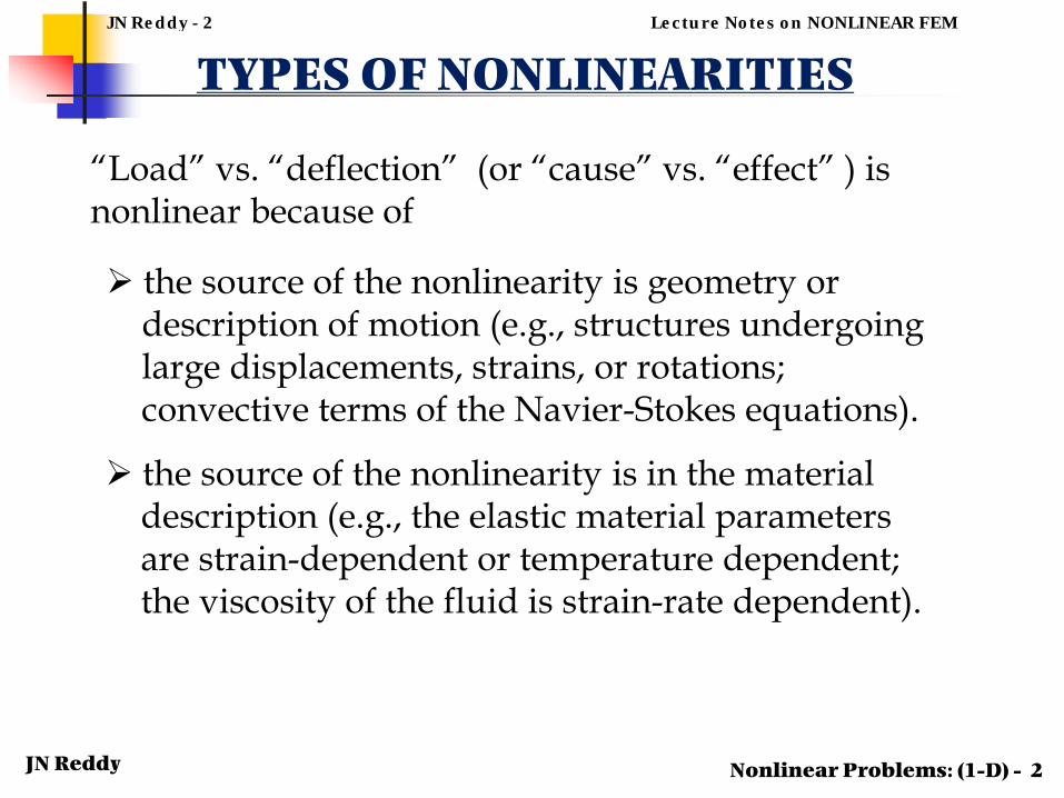
“Load” vs. “deflection” (or “cause” vs. “effect” ) is nonlinear because of

the source of the nonlinearity is in the materialdescription (e.g., the elastic material parametersare strain-dependent or temperature dependent;the viscosity of the fluid is strain-rate dependent).

the source of the nonlinearity is geometry or description of motion (e.g., structures undergoinglarge displacements, strains, or rotations;convective terms of the Navier-Stokes equations).

Nonlinear Problems: (1-D) - 2


JN Reddy Nonlinear Problems (1-D) : 3

( , ) ( , ) ( , ) ( ), 0

where ( / )

( , , ), ( , , ), ( , , )x

x x x

d du dua x u b x u c x u u f x x L

dx dx dxu du dx

a a x u u b b x u u c c x u u

MODEL 1-D PROBLEM

n

h j jj

u x u x u x1

Approximate solution: ( ) ( ) ( )

Weak Form

a

a

( ) ( )

( ) ( )

0b

a

b a

a b

xi h h

i i h i i a i b bx

x xi h h

i i h i i a i b bx x

dw du dua bw cw u w f dx w x Q w x Q

dx dx dx

dw du dua bw cw u dx w f dx w x Q w x Q

dx dx dx

Model Equation



FINITE ELEMENT MODEL

1( ) ( ), ( )

ne e e eh j j i i

ju x u x w x

=

= =∑

1

1

K u u F

( ) ( )

( ) ( )

b

a

b

a

ne e e e e e eij k j i

j

e eex j je e e eiij e e i e i jx

xe e ei e i i a i b nx

K u u F

d ddK a b c dxdx dx dx

F f dx x Q x Q

=

= ⇒ =

= + +

= + +

∑

∫

∫

11

0 a( ) ( )

( ) ( )

b a

a b

b a

a b

x xi h h

i i h i i a i b bx x

n x xj j e eij i i j i i a i b nx xj

dw du dua bw cw u dx w f dx w x Q w x Qdx dx dx

d ddu a b c dx f dx x Q x Qdx dx dx

=

= + + − + + ⋅

= + + − + +

∫ ∫

∑ ∫ ∫



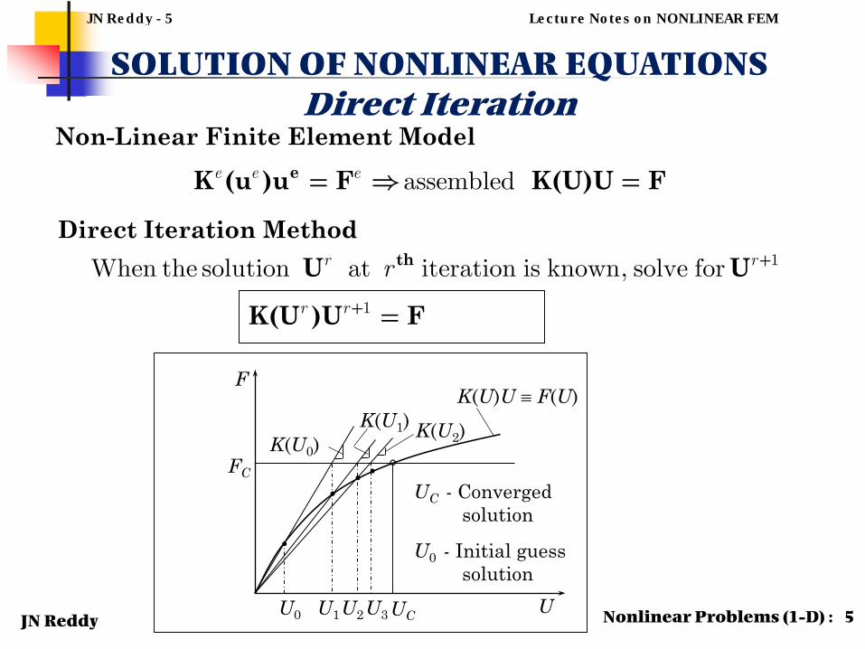
SOLUTION OF NONLINEAR EQUATIONSDirect Iteration

Direct Iteration Method

Non-Linear Finite Element ModeleK (u )u F K(U)U Fassemblede e e

r r

r r

r 1

1

When the solution at iteration is known, solve for

th U U

K(U )U F

K(U)U ≡ F(U)F

U

FC

UCU0

K(U0)

U1

K(U1)

U2

K(U2)

•

•• •

U3

°UC - Converged

solution

U0 - Initial guesssolution



SOLUTION OF NONLINEAR EQUATIONS(continued)

Direct Iteration Method

Convergence Criterion

Possible convergence

21

1

21

1

specified tolerance

NEQr rI I

INEQ

rI

I

U U

U

th U U

K(U )U F

1

1

Solution at iteration is known and solve forr r

r r

r



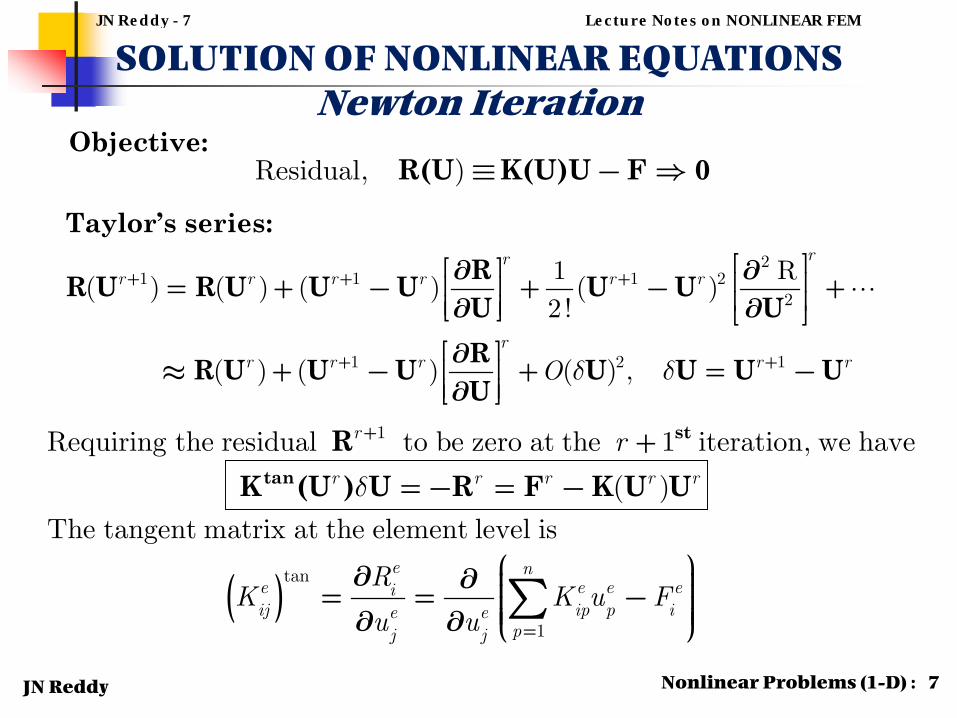
SOLUTION OF NONLINEAR EQUATIONSNewton Iteration

Taylor’s series:RR U R U U U U UU URR U U U U U U UU

21 1 1 2

2

1 2 1

1 R( ) ( ) ( ) ( )

2 !

( ) ( ) ( ) ,

rrr r r r r r

rr r r r rO

1

tan

1

Requiring the residual to be zero at the 1 iteration, we have

( )

The tangent matrix at the element level is

r

r r r r r

e ne e e eiij ip p ie e

pj j

r

RK K u F

u u

st

tan

R K (U ) U R F K U U

Residual, ) R(U K(U)U F 0Objective:



SOLUTION OF NONLINEAR EQUATIONSNewton-Raphson Iteration (continued)

T U U F K U U U U U1( ) ( ) ,r r r r r r

tan

1 1

en neipe e e e e e ei

ij ip p i ij p ije e ej j jp p

KRK K u F K u T

u u u

K(U) U − F ≡ R(U)F

U

FC

U0

T(U0)

T(U1)

T(U2)

•

••

UC = U3

°UC - Converged

solution

U0 - Initial guesssolutionδ U1 δ U2

U1 = δ U1 + U0 U2 = δ U2 + U0


JN Reddy 2-D Problems: 9

COMPUTATION OF TANGENT MATRIX COEFFICIENTS

1

1( ) ( )

( ) , b

a

b

a

e en ex j je e e e e e eiij k j i ij e e i e i jxj

xe e ei e i i a i b nx

d ddK u u F K a b c dxdx dx dx

F f dx x Q x Q

=

= = + +

= + +

∑ ∫

∫

tan

1 1

en neipe e e e e e ei

ij ip p i ij p ije e ej j jp p

KRK K u F K u T

u u u

Given: 0( , ) ( ) ( )e e ee u ux

dua x u a x a u x adx

= + +

Compute:e

ijT

EXERCISE:


JN Reddy

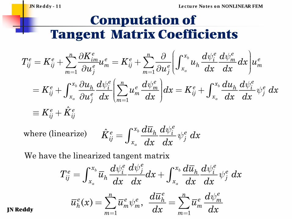
Computation of Tangent Matrix Coefficients

1

1

b

a

b

a

eenx je e e iij k kx k

een x je e ik kxk

ddK u dxdx dx

ddu dxdx dx

0

0

0 1

1

, ;

ˆ ˆ, ( )x

d duu f xdx dx

duu Q u udx

An Example:


JN Reddy

Computation of Tangent Matrix Coefficients

1 1

1

ˆ

b

a

b b

a a

e e en n xe e e e eim i mij ij m ij h me e xm mj j

e e enx xe e e eh i m h iij m ij jex xmje eij ij

K d dT K u K u dx uu u dx dx

u d d du dK u dx K dxu dx dx dx dx

K K

ˆ b

a

exe eh iij jx

du dK dxdx dx

where (linearize)

b b

a a

ee ex xje ei h iij jhx x

dd du ddx dxdx dx dx d

ux

T

We have the linearized tangent matrix

1 1

( ) ,e en n

e e e eh mh m m m

m m

du du x u udx dx


JN Reddy

PREPROCESSOR

PROCESSOR

POSTPROCESSOR

ECHOand

MESH1D

SOLVRUNSYM

ELMATRCS1D

INTERPLN1D

Post-processing

BNDRYUNS1D

FLOW CHART OF FEM1DUNSYM CODE

Computer Implementation: 12

JN Reddy

Assembly


JN Reddy

Flow Chart of a PROCESSOR Unit for Linear Analysis

Initialize global K and F

DO N = 1 to NEM

Call ELMATRCS to calculate K(N)

and F(N), and assemble to form global K and F

Transfer global information(material properties, geometry,

and solution) to element

Print solution STOP

Call BNDRYUNS1D to impose boundary conditions and call

SOLVRUNSYM to solve the equationsComputer Implementation: 13


JN Reddy

GENERAL LOGIC IN A COMPUTER PROGRAM for Nonlinear Analysis

Logic in the MAIN program

Initialize global Kij, fi

Iter = iter + 1

DO 1 to n

Iter = 0

Impose boundary conditionsand solve the equations

CALL ELMATRCS to calculate Kij(n)

and fi(n), and assemble to form global Kij and Fi

Transfer global information(material properties, geometry and solution)

to element

Iter < itmax

Error < ε yesno

STOP

Print Solution

Write a message

STOP

Yes No



JN Reddy

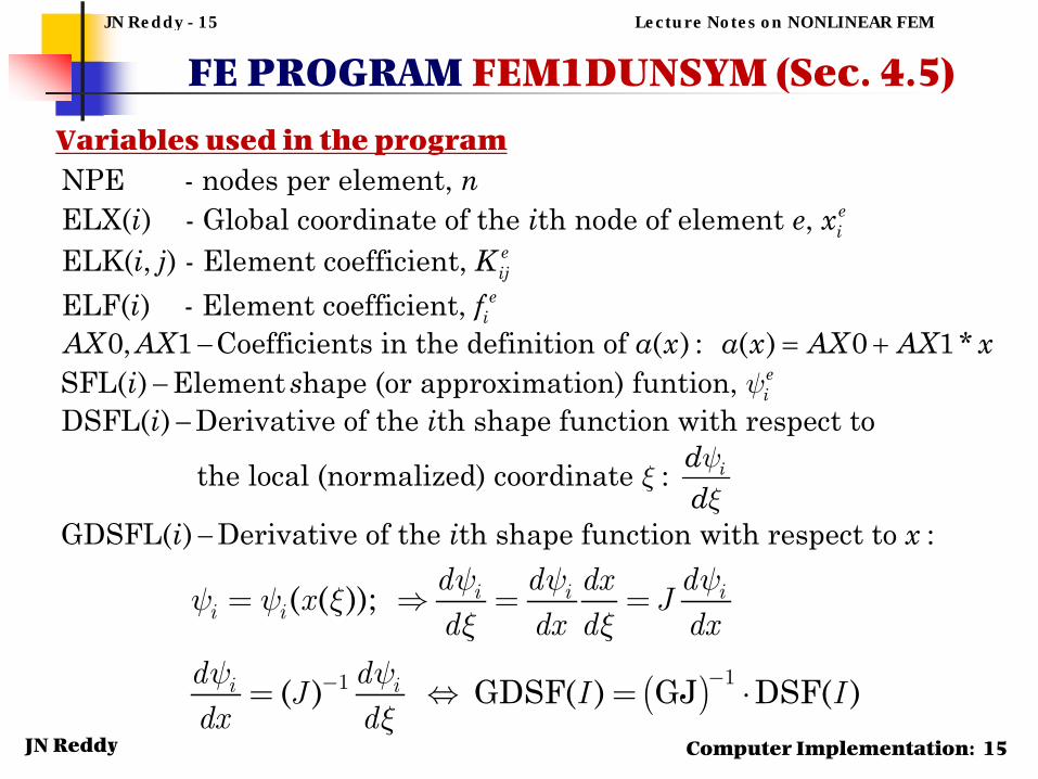
Variables used in the programNPE - nodes per element, ELX( ) - Global coordinate of the th node of element , ELK( , ) - Element coefficient, ELF( ) - Element coefficient,

0, 1 Coefficients in the definition o

ei

eij

ei

ni i e xi j Ki f

AX AX − f ( ) : ( ) 0 1*SFL( ) Element hape (or approximation) funtion, DSFL( ) Derivative of the th shape function with respect to

the local (normalized) coordinate :

GDSFL( ) Derivative of the

ei

i

a x a x AX AX xi s

i idd

i

= +−

−

− th shape function with respect to : i x

FE PROGRAM FEM1DUNSYM (Sec. 4.5)


( ( ));

( ) GDSF( ) GJ DSF( )

i i ii i

i i

d d ddxx J

d dx d dx

d dJ I I

dx d

11


JN Reddy

1

1

1 1

1 1 1( ) ( )

ˆ ˆ( ) GAUSPT( , ) * ( , )

1 1ˆ ( ) ( ) ( )

b

a

xj ji

e e i e i jx

j jie i j e i e e

e e eNGP NGP

ij I I ijI I

j iij e i j e i e

e e

d dda b c dxdx dx dx

d ddc b a J dJ d J d J d

F W F I NGP GAUSWT J NGP

d dF c b aJ d J

−

= =

+ +

= + +

≈ =

= + +

∫

∫

∑ ∑1 ,

1 , or 0.5

( , ) thGauss point, ,for the -point Gauss rule( , ) thGauss weight, ,for the -point Gauss rule

je

e

i i ie e e

e

I

I

dJ

d J dd d dd dxdx J d J hdx dx d J d d

GAUSPT I j I jGAUSWT I j I W j

= = = = =

−−

Numerical Integration

FINITE ELEMENT PROGRAM FEM1D-2


1 1( ) ( ) * ( ),

n ne ej j

j jx x ELX j SFL j

= =

= =∑ ∑


JN Reddy

( , ) ( , ) ( , )

ˆ ( )

( ) ( ) ( ) ( )( ) ( ) CNST

CNST GJ * GAUSWT( )Define , , and as given in the problem (you may

1

b

a

x j jiij i i j

x

NGP

ij NI NINI

d ddK a u x b u x c x u dx

dx dx dx

F W

A GDSF I GDSF J B SF I GDSF J

C SF I DSF J

NI

A B C

assume a general form that is useful for a number of problems):


The following statement should be inside a do-loop on number of Gauss points:

FINITE ELEMENT PROGRAM FEM1D-3

0 1( , ) * * * dua x u ax ax x axu u axdudx


JN Reddy

SUBROUTINE ELMATRCS1D (IEL,NPE,NONLIN,F0) IMPLICIT REAL*8(A-H,O-Z) DIMENSION GAUSPT(5,5),GAUSWT(5,5) COMMON /SHP/ SFL(4),GDSFL(4) COMMON /STF/ ELK(3,3),ELF(3),ELX(3),AX0,AX1,

BX0,BX1,CX0,CX1,FX0,FX1,FX2C

DATA GAUSPT/5*0.0D0,−0.57735027D0,0.57735027D0,3*0.0D0,1 −0.77459667D0,0.0D0,0.77459667D0,2*0.0D0,−0.86113631D0,2 −0.33998104D0,0.33998104D0,0.86113631D0,0.0D0,3 −0.906180D0,−0.538469D0,0.0D0,0.538469D0,0.906180D0/

DATA GAUSWT /2.0D0,4*0.0D0,2*1.0D0,3*0.0D0,0.55555555D0,1 0.88888888D0,0.55555555D0,2*0.0D0,0.34785485D0,2 2*0.65214515D0,0.34785485D0,0.0D0,0.2369227D0,3 0.478629D0,0.568889D0,0.478629D0,0.236927D0/

C

SUBROUTINE ELMATRCS1D-1(see pages 196-198 of the text book)

Nonlinear 1D problems: 18


JN Reddy

NGP=IEL+1EL=ELX(IEL+1)-ELX(1) DO 10 I=1,NPE

ELF(I)=0.0 DO 10 J=1,NPEIF(NONLIN.GT.1)THEN

TANG(I,J)=0.0ENDIF

10 ELK(I,J) = 0.0 DO 50 NI=1,NGP XI=GAUSS(NI,NGP) CALL INTERPLN1D (ELX,GJ,IEL,NPE,XI) CNST=GJ*WT(NI,NGP) X=0.0U=0.0 DU=0.0 DO 20 I=1,NPE X=X+SFL(I)*ELX(I)

20 CONTINUEAX=AX0+AX1*XBX=BX0+BX1*XCX=CX0+CX1*XFX=FX0+FX1*X+FX2*X*X

1 1

n ne ei i

i ix x ( ) ELX(i) * SFL(i)

( ) 0 1* *

( ) 0 1* 2 * *

a x AX AX x AXU u

f x FX FX x FX x x

= + +

= + +

* * ( )NICNST J w GJ GAUSWT NI= =

( , )NI GAUSPT NI NGP=ξ

Nonlinear 1D problems: 19

SUBROUTINE ELMATRCS1D-2JN Reddy - 19 Lecture Notes on NONLINEAR FEM

JN Reddy

IF(NONLIN.GT.0)THENU=0.0 DU=0.0 DO 20 I=1,NPE U=U+SFL(I)*ELU(I)DU=DU+GDSFL(I)*ELU(I)

20 CONTINUEAX=AX0+AX1*X+AU1*U+AUX1*DU+AU2*U*U+AUX2*DU*DUBX=BX0+BX1*X+BU1*U+BUX1*DU+BU2*U*U+BUX2*DU*DUCX=CX0+CX1*X+CU1*U+CUX1*DU+CU2*U*U+CUX2*DU*DUIF(NONLIN.GT.1)THEN

AXT1=(AU1+2.0*AU2*U)*DUAXT2=(AUX1+2.0*AUX2*DU)*DUBXT1=(BU1+2.0*BU2*U)*DUBXT2=(BUX1+2.0*BUX2*DU)*DUCXT1=(CU1+2.0*CU2*U)*UCXT2=(CUX1+2.0*CUX2*DU)*U

ENDIFENDIF

1 1( ) ( ) * ( )

n ne ei i

i iu u ELU i SFL i

= =

= =∑ ∑ψ ξ

Define parts of a, b, and cthat depend on u and du/dx

SUBROUTINE TO CALCULATE ELEMENT COEFFICIENTS-3

22

( , ) 0 1 * 1 * 1 *

2 * ( ) 2 *

dua x u AX AX x AU u AUXdx

duAU u AUXdx

= + + +

+ +


JN Reddy

DO 40 I=1,NPE ELF(I)=ELF(I)+FX*SFL(I)*CNST

DO 40 J=1,NPE S00=SFL(I)*SFL(J)*CNSTS10=GDSFL(I)*SFL(J)*CNST S11=GDSFL(I)*GDSFL(J)*CNST ELK(I,J)=ELK(I,J)+AX*S11+BX*S01+CX*S00IF(NONLIN.GT.1)THEN

TANG(I,J)=TANG(I,J)+AXT1*S10+AXT2*S11+BXT1*S00* +BXT2*S01+CXT1*S00+CXT2*S01

ENDIF40 CONTINUE 50 CONTINUE

1

1 1

b

a

x

ix

NGP

iNI

f ( x ) dx

f ( ) ( ) J d FX * SFL( i)* CNST

[ ]1

( , ) ( , ) ( , )

* 11 * 01 * 00

b

a

x j jii i jx

NGP

NI

d dda x u b x u c x u dxdx dx dx

AX S BX S CX S

=

+ +

= + +

∫

∑Nonlinear 1D problems: 20


1( , ) n ik

kkj

KTANG i j uu=

∂≡

∂∑


JN Reddy Nonlinear 1D problems: 22

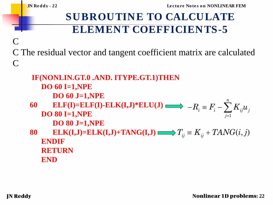
CC The residual vector and tangent coefficient matrix are calculatedC


IF(NONLIN.GT.0 .AND. ITYPE.GT.1)THEN DO 60 I=1,NPE

DO 60 J=1,NPE 60 ELF(I)=ELF(I)-ELK(I,J)*ELU(J)

DO 80 I=1,NPE DO 80 J=1,NPE

80 ELK(I,J)=ELK(I,J)+TANG(I,J)ENDIF RETURN END

1

n

i i ij jj

R F K u=

− ≡ − ∑

( , )ij ijT K TANG i j≡ +



MAIN PROGRAMUPDATING AND SAVING SOLUTIONS

CALL SLVUNSYM(GLK,MXNEQ,MXFBW,NEQ,NHBW) IF(NONLIN.EQ.0 .OR. NCOUNT.EQ.1)THEN

WRITE(IT,395)F0WRITE(IT,350)(GLK(I,NBW),I=1,NEQ) IF(NONLIN.EQ.0)THEN

STOPENDIF

ENDIF C Previous iteration solution is saved and current solution is updated

DO 210 I=1,NEQ GP2(I)=GP1(I) IF(ITYPE.LE.1)THEN

GP1(I)=GLK(I,NBW)ELSE

GP1(I)=GP1(I)+GLK(I,NBW)ENDIF

210 CONTINUE



C Test for the convergence of the solution DNORM=0.0 DINORM=0.0 DO 220 IE=1,NEQ DNORM=DNORM+GP1(IE)*GP1(IE)

220 DINORM=DINORM+(GP1(IE)-GP2(IE))*(GP1(IE)-GP2(IE))TOLR=DSQRT(DINORM/DNORM) IF(TOLR.GT.EPS)THEN

WRITE(IT,440)ITER,TOLR WRITE(IT,350)(GP1(I),I=1,NEQ) GOTO 80

ELSEWRITE(IT,400)NL,F0 WRITE(IT,420)ITER,TOLR WRITE(IT,350)(GP1(I),I=1,NEQ)

ENDIF270 CONTINUE

STOP

MAIN PROGRAM: ERROR CHECKJN Reddy - 24 Lecture Notes on NONLINEAR FEM

JN Reddy

NSPV – Number of specified primary variables of the problem.

ISPV(I,J) – Array containing the information about the global node number and the local

degree of freedom that is specified.

ISPV(I,1) – For the Ith boundary condition, the global node number at which the BC is specified.

ISPV(I,2) – For the Ith boundary condition, the local degree of freedom that is specified.

VSPV(I) – The specified value of the deg. of freedom.

Similar meaning for NSSV, ISSV, and VSSV for specified secondary variables

IMPOSOITION OF BOUNDARY CONDITIONS



JN Reddy

•

•

••

•

•

•

•• •

•

•••

•

• •• •

•

••

•

•

• • •••

• •••

••

••

•

•NDF = 36

I

16 17 18, ,U U U

1 2 3

1

, ,( ) *

K K KU U UK I NDF

•NDF= number of primary degrees of freedom at a node

IMPOSOITION OF BOUNDARY CONDITIONS



JN Reddy Computer program FEM1D 27

a11 a12 . . . a1k 0 0 0 . . . 0

a21 a22 . . . a2k a2k+1 0 0 . . . 0

a31 a32 . . . a3k a3k+1 a3k+2 0 0 . . .

. . . . . . . . .

0 . . . 0 an1 . . . ank . . . ann

[K] = [K] =(half-banded

form)

a11 a12 . . . a1k

a22 a23 . . . a2k+1

a33 a34 . . . a3k+2

. . . . . . .

NHBW

ann 0 . . . 0

an-1, n-1 an-1, n...0

NHBW

NEQ = n

Main diagonal

Last diagonal beyond which all coefficients are zero

NEQ

NEQ × NEQ

BANDED SYMMETRIC SYSTEM (used in FEM1D)

BANDED UNSYMMETRICSYSTEM

a11 a12 . . . a1k 0 0 0 . . . 0

a21 a22 . . . a2k a2k+1 0 0 . . . 0

a31 a32 . . . a3k a3k+1 a3k+2 0 0 . . .

. . . . . . . . .

0 . . . 0 an1 . . . ank . . . ann

[K] = [K] =(full-banded

form)

NHBW NBW=2*NHBW

NEQ = n

Main diagonal

Last diagonal beyond which all coefficients are zero

NEQ

NEQ × NEQ

11 12 1* * * ka a a

21 22 23 2( 1)* * ka a a a +

31 32 33 34 3( 2)* ka a a a a +

41 42 43 44 45 4( 3)ka a a a a a +

( 1) * * *n n nna a−

##..##

NBWth column;used for storing F

FORMATS OF ASSEMBLED EQUATIONSJN Reddy - 27 Lecture Notes on NONLINEAR FEM

JN Reddy

0 0

0 500 300

d dTk T x Ldx dx

T T L° °

− = < < = =

( ) ,

( ) K, ( ) K

Example 1: 1-D Heat flow

( ) 3 10 1 0 11 0 2 2 10k T k k T k k K− ° −= + = = ×°( ) , . W/ (m K),

DI/NI Direct iteration Newton iterationx Linear 8L 4Q 8L 4Q

0.0000 500.00 500.00 500.00 500.00 500.000.0225 475.00 477.24 477.24 477.24 477.240.0450 450.00 453.94 453.94 453.94 453.940.0675 425.00 430.06 430.06 430.05 430.050.0900 400.00 405.54 405.54 405.54 405.540.1125 375.00 380.35 380.35 380.34 380.340.1350 350.00 354.40 354.40 354.40 354.400.1575 325.00 327.65 327.65 327.65 327.650.1800 300.00 300.00 300.00 300.00 300.00


JN Reddy

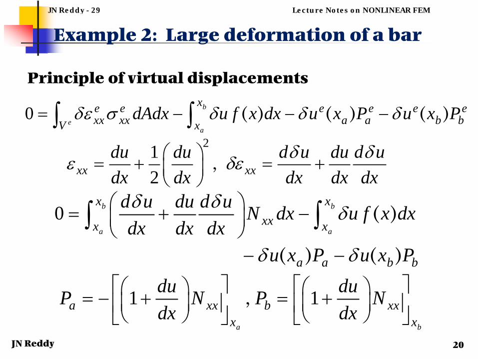
Example 2: Large deformation of a bar

0 b

ea

xe e e e e exx xx a a b bV x

dAdx u f x dx u x P u x Pδε σ δ δ δ= − − −∫ ∫ ( ) ( ) ( ) 21

2xx xxdu du d u du d udx dx dx dx dx

δ δε δε = + = +

,

Principle of virtual displacements

0 ( )

( ) ( )

b b

a a

x xxxx x

a a b b

d u du d u N dx u f x dxdx dx dx

u x P u x P

δ δ δ

δ δ

= + −

− −

∫ ∫

1 1a b

a xx b xxx x

du duP N P Ndx dx

= − + = + ,

20


JN Reddy

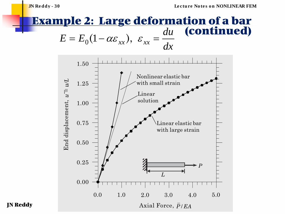
Example 2: Large deformation of a bar(continued)

0 1 xx xxduE Edx

αε ε= − =( ),

PL

2.0 3.0 4.0Axial Force, P / EA

Nonlinear elastic bar with small strain

Linear solution

Linear elastic bar with large strain

0.0 1.0 5.0

1.25

1.00

0.75

0.50

0.25

0.00

1.50E

nddi

spla

cem

ent,

u =

u/L


JN Reddy 31

Finite element formulation of a 1-Dmodel nonlinear problem

Solution of nonlinear equations (Picard and Newton) Calculation of tangent matrix coefficients General logic in a computer program Numerical examples Nonlinear (material) nonlinear analysis of

a 1D heat transfer problem Nonlinear (geometric and material) analysis of

a bar problem

SUMMARYJN Reddy - 31 Lecture Notes on NONLINEAR FEM

read: chapter 4 contents - tamu mechanics

Documents