real risks: statistical thinking and risk perception · real risks statistical thinking and risk...

Digital Publication

Digital Publication

Digital PublicationFRASER INSTITUTE

December 2007

Real RisksStatistical Thinking and Risk Perception

Mark Wolters

The Fraser Institutewww.fraserinstitute.org

Contents

Overview of risk and statistical thinking / 1

1 A tour of the risk landscape / 1

2 A case study of Canadian mortality data / 5

Conclusion / 10

Introduction / 11

Statistical thinking / 11

This publication / 12

1 Risk, society, and individual decision making / 14

Risk is a complex system / 14

The problem of risk perception / 16

Institutional and individual perspectives / 18

Risks old and new / 19

Back to statistical thinking / 20

2 Statistical thinking and Canadian mortality data / 22

The data set / 22

Life expectancy / 23

Causes of death / 30

Conclusion / 38

Appendix: Methodological Notes / 40

List of causes of death / 40

Ordinary life table / 44

References / 47

About the author & Acknowledgments / 50

Publishing information / 51

About The Fraser Institute / 52

Supporting The Fraser Institute / 53

1


Real Risks

Overview of risk and statistical thinking

In today’s information age, consumers are exposed to an unprecedented amount of messaging in daily life. From moment to moment, we endure a steady bombardment of advertising, news items, political views, and other information intended to help us make decisions toward happier, healthier lives. Conveniently, much of the information we consume about health and wellness is prepackaged for easy digestion. Elaborate scientific studies are distilled into snappy sound bites—“Studies show that Disease X kills 2.7 people per minute”—while exhaustive research and development behind a new product is spun into glossy advertising copy—“Ask your doctor about Condition Y, which affects up to 20,000 people each year”.

Statistics such as these are common and familiar, and they appear to contain important information for consumers. Most people understand that statistical analy-sis is used to summarize a set of data, identify trends, and confidently project the probability—or risk—of a particular event or outcome. But how relevant are statistics to our individual experience? Are we at serious risk of contracting Disease X or devel-oping Condition Y? How much should we worry about these risks in the context of our everyday lives? Our inherent desire to understand the myriad risks to our health drives many of the everyday decisions we make, from lifestyle choices to consumer patterns to political views. But much of the information we receive about risk is derived from the painstaking mathematical analysis of large and complex sets of information, which requires an expertise that is well beyond the grasp of most people.

Yet non-statisticians can take heart. While there is much more to statistics and risk than meets the eye, we can easily extract meaningful information from a set of data by asking the right questions. Once we gain an appreciation of how risk informa-tion can be interpreted—and misinterpreted—we can begin to make informed deci-sions about our own health and that of our society.

1 A tour of the risk landscape

Statistical thinkingSuppose you see a news story reporting that ten people across Canada were killed by lightning last year while playing golf. Assuming a population of 30 million Canadians, that is a death rate of one in three million. Is this worth worrying about? This depends first on the validity of the information: are ten deaths per year typical or was there a rash of lightning strikes on golf courses last year? Did the deaths occur randomly across the country or did nine of them happen at Treeless Acres Golf Club at the top of beautiful Mount Stormy?

2


Real Risks

The “worry factor” of this risk information also depends on individual behaviour: non-golfers have little to be concerned about but people who get a thrill out of golfing during thunderstorms should consider this information carefully. Finally, even if you have reason to worry, is your lifetime risk of being struck by lightning while golfing any greater than, say, the risk of dying in a car accident while driving to the golf course? If you know only that ten people died from lightning strikes last year while golfing, there is no way to put this information into useful perspective.

When presented with new information about risk such as the fictitious example above, we can choose to believe it and act accordingly or we can investigate it and draw our own conclusions. Fortunately, an education in applied mathematics is not necessary to make sense of the morass of risk-related statistics available to consum-ers. Rather, the practice of statistical thinking—built on basic, non-mathematical con-cepts of statistics—can easily help one assess risk critically in the face of uncertainty. Statistical thinking involves two key concepts:

l understanding the process by which the information (or data) is collected; and l presenting conclusions drawn from the data in an appropriate context (conclusions

reported out of context are frequently misleading).

The example above illustrates the main questions involved in statistical thinking. By what process was the risk data generated and reported? How will I be exposed to this risk? How does the risk vary according to my behaviour? How can I compare other risks to the risk in question?

Interpreting risk in the golf example may seem obvious or trivial but a real set of mortality data does require a serious effort in statistical thinking. In part 2 of this publication (p. 22), a case study of Canadian mortality data illustrates in detail how statistical thinking (“What is the process? What is the context?”) can be applied to interpret risk accurately from a complex but highly relevant set of information.

Risk in societyNaturally, consumers are not the only members of society who are risk averse. Being a gullible consumer of risk information can lead to bad decision-making at the individ-ual level but it can also spawn wanton wastefulness with unintended consequences at the societal level. Identifying, assessing, and managing risks in society requires a com-plex system with many stakeholders. Any public, risk-related issue involves regulatory bodies that control risk-management policy; scientists who attempt to understand the risks better; corporate stakeholders with a fiscal responsibility; special-interest groups that attempt to influence the debate; and media outlets that seek to present an objec-tive viewpoint while maintaining their own bottom line. In addition, two types of chance events can also influence the interactions among stakeholders: chance events

3


Real Risks

that affect individuals (such as a loved one contracting a particular disease), and chance events that act on a societal scale (such as an epidemic or a chemical spill).

The web of interactions among these varied stakeholders can produce complex responses to risk, ranging from unpredictable to irrational behaviour. The way in which stakeholders react to risk is difficult to predict, and helps to explain the common lack of consensus about risk-related issues. For this reason, many risk-management policies are perceived as ineffective.

How we perceive riskAmidst the scrum of institutional stakeholders, the individual maintains a powerful role in the complex system of risk management. People are at the heart of every orga-nization involved in assessing, communicating, and managing risk. Each person is influenced by a unique set of values, biases, and experiences, which collectively deter-mine how they perceive and respond to a particular risk. Risk perception is a personal and informal assessment of risk that is based on intuition, experience, and whatever information is at hand. Risk perception often differs drastically from the formal risk-assessment process of governments and other large institutions. Indeed, our some-times irrational individual responses to a perceived risk can lead to poor public choices, with negative consequences for society.

One example of this is the ongoing debate over nuclear power generation and its associated public health risks. Despite expert assurances that nuclear power is extremely safe, many people remain vehemently opposed to it. Why? Because the tech-nology is conceptually connected to radiation and to nuclear weapons, and because high-profile disasters such as Three-Mile Island and Cherynobyl suggest a potential for future catastrophes. These connections inspire fear, which powerfully influences perceived risk. Because the average person does not understand the physics behind the issues well enough to assuage their mistrust of the industry, the objective evidence supporting nuclear power has little effect on risk perception.

Finally, the potential impact of the media in influencing risk perception should not be understated. The media often report only the substantive conclusions of a scien-tific study, failing to include information about process and context. This is not objec-tive reporting; it is an incomplete account that burdens the individual with interpreting the information without knowledge of its validity or limitations. Of course, a media outlet with its own agenda may even report risk information in a deliberately selective or distorted fashion.

In bridging the gap between risk assessment and risk perception, some argue that the public simply needs to be “educated” to agree with the experts. Others view risk perception as more inclusive and forward-thinking than expert assessment. The ongoing resolution of expert risk assessment and public risk perception is one of the great challenges of risk management.

4


Real Risks

Managing riskAs a duty to shareholders and the public, large institutions and governments must consider problems of risk using formal, standardized, and defensible procedures. Risk assessment ensures that institutions are at least partially accountable for mitigating risks to the public. For instance, cyclists may applaud a government that spends mil-lions to fill potholes but, if that same government neglects to provide clean water to its citizens, it is not serving the public interest by effectively assessing or managing risks.

Typically, a risk assessment first gathers objective information about the prob-ability and severity of a given risk. Next, decisions are made about how to manage the risk, weighing factors such as cost-benefit, available alternatives, institutional val-ues, and so on. Conversely, we manage risks at the individual level by making dozens of small, personal decisions each day that are based on our values and the risks we perceive to ourselves and our loved ones. Perception dominates decision-making for individuals much more than it does for institutions, simply because individuals are real people with jobs, families, and things to do. We have less time, less information, and less training for performing analysis.

Naturally, the way in which individuals and the public perceive risk does not always agree with the institutional assessment of risk, which can lead to serious conflict. Suppose public opinion is overwhelmingly concerned with a relatively minor public health risk, such as the potholes in the previous example. What should the government do? Can it convince the public of an alternative action through communication, educa-tion, and persuasion? If not, should it force an alternative on the unwilling electorate or should it respect the will of the people and begin street repairs? There is no easy solution; the difference in perception between institutions and the public highlights some of the fundamental issues about the nature of our society.

New and historical risksIn our quest for a better understanding of risk as it applies to ourselves and to society, we can distinguish between two types of risk: historical and new risks. A historical risk describes an event or outcome that has occurred frequently enough for a significant amount of data to have been collected over the years, making it possible to estimate with reasonable accuracy the danger it poses. For example, thousands of deaths from cardiovascular disease and car accidents are recorded each year. Not only do we under-stand the mechanisms that cause them to occur but the available data also documents their impact in society.

New risks are either hypothetical or rare and it is often unclear how much actual danger they present. New risks may include rare catastrophic events with little or no precedent (such as severe global warming, meteor impacts, or full-scale nuclear war), or they could be low-level impacts that are predicted across a population but are difficult to observe (such as cancers caused by food additives and household chemicals). Over

5


Real Risks

time, a new risk may become a historical risk once enough information is gathered; the risk of cancer associated with cigarette smoking is an example.

It can be fairly straightforward to estimate the probability of a historical risk based on the available information. New risks require a more involved process, in which the event is broken down into its parts and studied, then recombined through a model to predict the behavior of the whole. This process requires more focus on basic science, more assumptions made, and more debate about which models to use. For example, scientists often determine the cancer-causing potential of a new substance by giving enormous doses to rats or mice. Applying these results to humans involves two extrapolations: jumping the species barrier from rodents to humans and using the results of large and deliberate doses to estimate the effects of small and incidental doses. As a result, relying on toxicological studies alone to estimate the cancer-causing potential of a substance can lead to uncertainty about its actual risk to humans.

Despite their obvious differences, new and historical risks have much in com-mon. Both are reported in the news, both are reported with statistics, and both are significantly affected by people’s risk perception and media bias. The burden of inter-pretation shifts to the individual: accept the message as issued or interpret the infor-mation in the larger context of risk in their lives and in society.

2 A case study of Canadian mortality data

Consider this true statement: 16,490 deaths in Canada were attributed to renal failure between 2000 and 2004. How significant is this number? We can put this information into better context once we appreciate the number of deaths from pancreatic cancer (16,505), suicide (18,326), and motor-vehicle accidents (13,910) over the same period. Even with this knowledge, it is worthwhile to ask what the risk is of renal failure at dif-ferent ages, what the factors are that put one at risk of renal failure, and how the risk of renal failure compares to other risks.

Our attitudes and decisions toward risk affect not only our own health but also the way in which risks are prioritized and managed in society. Statistical thinking pro-vides a useful road map for assessing risk but how does one use statistical thinking to make sense of real and complex risk information? The following case study analyzes a set of Canadian mortality data in an attempt to illustrate how one might interpret risk information in a meaningful and relevant way.

All deaths in Canada are registered by age and cause, using the World Health Organization’s International Classification of Diseases (ICD) system. This hierarchi-cal system uses thousands of alphanumeric codes that correspond to a specific dis-ease, condition, or event leading to death. For example, accidents are assigned codes V01 to X59; transport accidents form a subgroup (V01–V99); injuries to cyclists form

6


Real Risks

a further subgroup (V10–V19); and so on, down to specific instances such as “Pedal cyclist injured in collision with pedestrian or animal, passenger injured” (V11.5).

Each year, Statistics Canada reports mortality data based on the ICD codes and grouped into 113 broad causes. The 113 causes may be further grouped into fewer cat-egories for convenience; for example, 24 of the 113 causes of death are cancers. The number of deaths due to each cause is also recorded by age. For the purposes of this example, the mortality data from 2000 to 2004 has been aggregated to produce a single data set. By combining this information with data from Canada Census, we can esti-mate the probability of death by different causes, at any age. We can further use these probabilities to calculate life expectancy and other useful information. In this way, the Canadian mortality data can be used to inform people of the real risk associated with various causes of death, which is a starting point for making personal decisions about risk management.

Statistical thinking and life expectancyHow long can a person expect to live? Using mortality data and census information, we can construct a so-called ordinary life table (OLT) that yields a measure of average life expectancy, or the estimated number of additional years a person will live, as a func-tion of their current age. In popular discussion, the single value from an OLT that is most commonly reported is average life expectancy at birth. Based on our aggregated mortality data from 2000 to 2004, this value is 79.8 years. [table 1]

Does this statistic apply to everyone in Canada? Using statistical thinking, let’s examine how the statistic is generated and reported, and its underlying assumptions. Our statistic of 79.8 years is the life expectancy at birth, not the age to which the average adult, who has already lived several decades, can expect to live. With every year we survive, we have avoided many risks that could have killed us. Another look

Table 1: Life expectancy (years) in Canada, based on aggregated mortality data

from 2000 to 2004

Age Life Expectancy

Age Life Expectancy

Age Life Expectancy

0 79.8 35 46.0 65 19.1

5 75.2 40 41.2 70 15.3

10 70.3 45 36.4 75 12.0

15 65.3 50 31.8 80 9.0

20 60.5 55 27.4 85 6.6

25 55.6 60 23.1 90 4.7

30 50.8

Sources: Statistics Canada 2004, 2006a, 2006b, 2006c, 2006d, 2006e, 2007; calculations and analysis by author.

7


Real Risks

at the OLT shows that a 50-year-old can expect to live an additional 31.8 years for an average age of death of 81.8. For those that survive to age 80, the average age-of-death increases to 89.

Furthermore, the OLT is based on a critical assumption that the death rates for all ages and for all causes will be constant throughout all future time; that is, that they will be the same 100 years from now as they are today. This is fine for the purpose of producing a table but, in the real world, advances in science and technology constantly increase our longevity. In this light, our life-expectancy statistic simply provides a snapshot of the Canadian population as it was from 2000 to 2004.

Finally, we must remember that our life-expectancy statistic is an average based on an entire population. Yet no one is exactly average: these life-expectancy statis-tics describe a theoretical person who constantly shares the same risk for all diseases as everyone else and who, moreover, is half male and half female (our ordinary life table was constructed using aggregate data for both genders). Separate tables can be constructed for each gender and doing so confirms a familiar fact: females have con-siderably greater life expectancy than males. But the averaging of these two distinct subgroups concealed this important information.

Averages provide easily used summaries and are the type of statistic most com-monly encountered by the public. But, by quoting an average, an entire distribution of possible outcomes is distilled into a single, potentially misleading number. As our aggregate mortality data shows, an average population value such as life expectancy has less significance for an individual than one might expect at first glance. However, we can draw out the significance by looking beyond the average numbers to find age- and gender-specific statistics. For example, if we were to construct gender-specific ordinary life tables from our mortality data, we would find that men have a life expectancy at birth of 77.2 years while that value increases to 82.2 years for women. If we then plotted these gender-specific mortality rates against age, we would find that 90% of females and 84% of males are expected to reach age 65 but, beyond this age, men have a much higher mortality than women, producing the five-year gap in average life expectancy. This analysis is discussed in some detail in the main body of this publication.

Statistical thinking and causes of deathIn addition to providing useful information about life expectancy, our Canadian mor-tality data-set can also describe the risk of dying of a particular cause. We can use the data to create a multiple decrement life table (MDLT), a derivative of the ordinary life table. With this information we can answer a number of questions, such as the prob-ability of dying from a given cause or the life expectancy of a person who eventually dies of that cause.

Statistical thinking requires us to first consider the processes behind con-structing an MDLT. Like the ordinary life table, the MDLT provides a snapshot of

8


Real Risks

a population at a particular point in time (in this case, 2000 to 2004), and its results cannot be reliably transferred to future time. We must also consider the way in which deaths are counted, classified, and reported. If an elderly man has a heart attack while water skiing, should this be counted as a heart attack, or as a water-sports accident? Regardless of how it should be counted, how will it be counted once the deceased reaches the hospital? Will the reported cause of death for such a case be consistent over time and from hospital to hospital?

In Canada, deaths are classified in two stages: first, the death certificate is filled out (usually by a doctor); then, a medical coder uses the certificate to assign a single ICD code for the event. Inconsistencies in this process lead Statistics Canada to monitor the quality of the ICD information submitted, noting in a recent disclaimer that approximately one-third of death certificates contain errors. Such disclaimers in the mortality data highlight deficiencies in process and provide important context to the reader.

A limitation of the ICD system is that it provides little information about cause-and-effect relationships. For example, it is not possible to use this data set to study the relationship between smoking and lung cancer or to see how many deaths occur due to water skiing. The “effect” in question is always death and the “causes” are fixed by the system of codes used by the ICD.

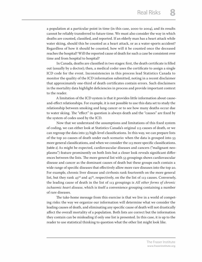
Now that we understand the assumptions and limitations of this fixed system of coding, we can either look at Statistics Canada’s original 113 causes of death, or we can regroup the data into 53 high-level classifications. In this way, we can prepare lists of the top 20 causes of death under each scenario: when the data is grouped into 53 more general classifications, and when we consider the 113 more specific classifications. [table 2] As might be expected, cardiovascular diseases and cancers (“malignant neo-plasms”) feature prominently on both lists but a closer look reveals significant differ-ences between the lists. The more general list with 53 groupings shows cardiovascular disease and cancer as the dominant causes of death but these groups each contain a wide range of specific diseases that effectively allow more rare diseases into the top 20. For example, chronic liver disease and cirrhosis rank fourteenth on the more general list, but they rank 43rd and 45th, respectively, on the the list of 113 causes. Conversely, the leading cause of death in the list of 113 groupings is All other forms of chronic ischaemic heart disease, which is itself a convenience grouping containing a number of rare diseases.

The take-home message from this exercise is that we live in a world of compet-ing risks: the way we organize our information will determine what we consider the leading causes of death, and eliminating any specific cause of death will not drastically affect the overall mortality of a population. Both lists are correct but the information they contain can be misleading if only one list is presented. In this case, it is up to the reader to use statistical thinking to question what the other list might look like.

9


Real Risks

Table 2: The top 20 causes of death, when all deaths are first grouped into 53 more general causes (left),

or when all deaths are first grouped into 113 more specific causes (right)

More general causes of death More specific causes of death

1 Major cardiovascular diseases All other forms of chronic ischaemic heart disease

2 Malignant neoplasms All other diseases (residual)

3 All other diseases (residual) Acute myocardial infarction

4 Chronic lower respiratory diseases Cerebrovascular diseases

5 Diabetes mellitus Malignant neoplasms of trachea, bronchus and lung

6 Accidents (unintentional injuries) Other chronic lower respiratory diseases

7 Alzheimer's disease All other and unspecified malignant neoplasms

8 Influenza and pneumonia Diabetes mellitus

9 Nephritis, nephrotic syndrome and nephrosis All other forms of heart disease

10 Symptoms, signs and abnormal clinical and laboratory findings, not elsewhere classified

Alzheimer's disease

11 Other diseases of respiratory system Malignant neoplasms of colon, rectum and anus

12 Intentional self-harm (suicide) Pneumonia

13 Parkinson's disease Heart failure

14 Chronic liver disease and cirrhosis Malignant neoplasm of breast

15 Septicaemia Malignant neoplasm of prostate

16 In situ neoplasms, benign neoplasms and neoplasms of uncertain or unknown behaviour

Renal failure

17 Pneumonitis due to solids and liquids Malignant neoplasm of pancreas

18 Certain conditions originating in the perinatal period Symptoms, signs and abnormal clinical and laboratory findings, not elsewhere classified

19 Anaemias Other and unspecified nontransport accidents and their sequelae

20 Certain other intestinal infections Other diseases of respiratory system

Source: Statistics Canada 2004, 2006a, 2006b, 2006c, 2006d, 2006e, 2007; calculations and analysis by author.

10


Real Risks

Conclusion

The concept of risk applies as much to our individual health and welfare as it does to that of society. We are exposed to competing risks throughout our lives, and acting to change our exposure to one risk will undoubtedly affect our level of exposure to others. At the societal level, decision-making about risk is the result of interactions between the public and its institutions, and is driven by a complex mix of fact and perception, knowledge and uncertainty, trust and skepticism, and cost and benefit.

However, it is the individual decision-maker who is the single largest consumer of information; what we think, know, and feel about risks plays a powerful role in the broader context of risk in society. It is easy to be swayed—for better or for worse—by statistics that we accept without question. As the Canadian mortality data illustrates, drawing one’s own conclusions from complex statistics demands a concerted effort to understand process and context and to compare one risk with the numerous other risks we are simultaneously exposed to. But when our own health and that of our loved ones is at stake, as well as the overall health of our society, asking the right questions of risk information can mean the difference between sickness and health, and life and death.

11


Real Risks

Introduction

A judicious man looks on statistics not to get knowledge, but to save himself from having ignorance foisted on him.

—Thomas Carlyle

Messages about risk are everywhere. A charity reminds us that disease X kills 2.7 peo-ple per minute; a pharmaceutical company suggests that we ask our doctor about con-dition Y, which affects up to 20,000 people annually (though most of them do not even know it); and a new study suggests that using technology Z may increase the chance of getting disease Q by over 40%. What do these numbers really mean?

When presented with these messages about risk, we have two options: to accept the messages or to seek more information. If we simply accept the messages, we may find ourselves getting out our chequebooks, swallowing the latest pill, or avoiding the newest gadget, with little real basis for our actions. If, on the other hand, we choose to investigate the facts behind the messages, we may find that “fact” is a more pliable concept than we thought. A little digging is likely to turn up numerous versions of the story—some from scientific organizations, some from government, and others from industry or special-interest groups. Comparing these accounts to each other, we are bound to find conflicting views. Depending on the issue, the conflicts may range from quibbles about interpretation to antagonistic contradiction about basic facts. Worst of all, each report is likely to be bolstered by an array of statistics that, when considered one at a time, inspire confidence; but when considered as a group, are sure to raise suspicion. Instead of clarity, this attempt to find more information will only gain the seeker a sense of confusion, along with a healthy contempt for statistics.

Statistical thinking

The suspicious feeling people get around statistics is generally well founded: it is, in fact, easy to be misled by statistics. As a result, many people feel that they may be missing something if they try to apply statistical information to their own lives. Fortunately, understanding a few concepts from statistics (the science) can help people make more sense of statistics (the numbers). The concepts in question are not mathematical in nature. They are a set of thinking skills, collectively called statistical thinking [Britz,

Emerling, Hare, Hoerl, and Shade, 1996; Wild and Phannkuch, 1999]. Broadly defined, statisti-cal thinking is the set of skills needed to assess information critically in the presence of uncertainty. It is a “data sense” that prevents a person from being misled by variability. Statistical thinking involves two key themes:

12


Real Risks

Process All information is the result of a process, and understanding the processes behind the information we receive is essential to meaningful interpretation.

Context All processes and, therefore, all data have variability and it is crucially important to understand any data in the context of variability appropriate to that data. [1]

Randomness also plays a large role in all of our lives. It is particularly important when considering risk because the very concept of risk implies chance and uncertainty; and because everyone has an interest in understanding the risks to their health and well-being. Although most of us desire to make good decisions regarding our health and welfare, many people are ill-equipped to deal with problems involving uncertainty and variability [Tversky and Kahneman 1974; Piattelli-Palmarini 1994]. Developing an ability to engage in statistical thinking is, consequently, useful in many aspects of life.

This publication

This publication aims to provide the reader with a gentle start at developing statistical thinking as it applies to the interpretation of risks. The theme of statistical think-ing will be developed in two stages. In Part 1, “Risk, society, and individual decision making,” the need for improved critical thinking will be motivated by looking at the high-level structure of the risk culture we live in. In Part 2, “Statistical thinking and Canadian mortality data,” we will demonstrate statistical thinking using Canadian mortality data.

Before moving on to the body of the discussion, a few conciliatory words are in order. The principles of statistical thinking are best illustrated through real examples; in particular, real-world risk controversies provide excellent illustrations. At the same time, an appreciation for statistical thinking fosters a desire to review any contro-versial issue from all angles before drawing conclusions: an example should properly be discussed in depth, to ensure fair treatment. This creates a predicament for the author of a short publication on statistical thinking: how to provide good illustrations of the principles, without undermining those same principles by resorting to a cursory, superficial analysis.

[1] The defining elements of statistical thinking vary somewhat depending on the author. Britz et al. [1996] discuss statistical thinking in the context of improving industrial processes while Wild and Phannkuch (1999) review it from a statistics education standpoint. The themes of process and context are proposed here as a most general statement of statistical thinking principles. Good sources of generally-applied examples of statistical thinking are Campbell [1974]; Balestracci [1998]; and Murray, Schwartz, and Lichter [2002]; as well as the website <http://www.stats.org>.

http://www.stats.org

13


Real Risks

The solution attempted here is to present only a very high-level summary of mortality data in Canada, to illustrate the desired concepts while skirting the most complicated individual issues. Although every effort has been made to ensure that the analysis is valid, there is no intention of providing detailed consideration of particu-lar risks or to endorse any specific risk-management policies. When considering the examples in the text, the reader is encouraged to focus primarily on the ways of think-ing about data. These habits of thought are the real subject of the publication.

Finally, although mortality will be discussed in broad terms at the population level, this is not meant to diminish the significance of any individual death, no matter the cause; nor is the focus on death statistics intended to diminish the importance of other factors, such as quality of life, in setting public-health priorities. Focusing on mortality at the population level always risks oversimplifying and dehumanizing the issues; but this perspective is necessary to help each of us understand how our own risks play out on the social stage.

14


Real Risks

1 Risk, society, and individual decision making

The majority is the best way, because it is visible, and has strength to make itself obeyed. Yet it is the opinion of the least able.

—Blaise Pascal

The outcome of any risk-related issue is determined by a complex mixture of fact and perception, knowledge and uncertainty, individuals and society, trust and skepticism, cost and benefit. In keeping with the two broad themes in statistical thinking of pro-cess and context, we must situate the individual decision-maker in the broader context of risk in society, and explore the processes that influence what we know, think, and feel about risks.

Risk is a complex system

The identification, assessment, and management of risks is a complex system involving many agents and information flows. For any risk-related issue, there are numerous players: regulatory bodies control risk-management policy; the scientific establishment attempts to understand risks better; competing advocacy groups attempt to influence the debate; and the media attempts to cover all of the develop-ments while meeting their own bottom line. In the middle of this stands the public, who are at once the object of the discussion, its subject, and the principal determi-nant of the outcome.

A key characteristic of a complex system is that predicting the behavior of the system as a whole is difficult, even if the workings of the constituent parts are well understood. The complex behavior of the system is a result of the network of inter-actions among the parts. In systems modeling, an influence diagram is sometimes used to visualize a complex system [Shachter, 1986]. Figure 1 shows a first attempt at creating an influence diagram for risk in society. In this simplified representation, four interacting agents are shown: individuals, the research establishment, the public, and policy makers. The influences these agents have on each other’s perceptions and activities are shown as arrows connecting them. Also shown are two types of random events that can have influence: chance events that affect individuals (such as a loved one contracting a particular disease), and chance events that act on a societal scale (such as an epidemic or a chemical spill).

The web of interactions among the various agents is what produces complex—unstable, unpredictable, or irrational—responses to risk. The exact nature of the inter-actions are hard to predict and there are many feedback loops in the system. The notion

15


Real Risks

of risk as a complex system can help to explain (or at least come to terms with) the lack of consensus about risk issues and the ineffectiveness of many risk-management poli-cies. Chance events of little real importance can have a disproportionate influence on policy through complex social interactions [Kasperson, Renn, Slovic, Brown, Emel, Goble,

Kasperson, and Ratick, 1988] and interventions that are enormously expensive on a cost-per-life-saved basis are implemented rather than interventions that are essentially free [Wilson and Crouch, 2001].

The real system through which risk is communicated, perceived, and managed is considerably more complex than the one shown in figure 1. Two important players are not shown on the diagram: corporate stakeholders and special-interest groups. Both of these agents strongly influence (and are influenced by) most of the other nodes on the graph—to the point where drawing these agents on the figure would produce a dense and unwieldy web of interconnections. Another major force not adequately portrayed in the figure is the media. In many cases, the news media are the means through which risk information is transmitted from one agent to another. The media, of course, can have their own agendas, so that information is transmitted in a selec-tive or distorted fashion. Influences largely transmitted by the media are shown as dashed arrows in the figure; the potential impact of the media on the system should not be understated.

Figure 1: Influence diagram of risk in society

Note: This is a simplistic influence diagram of risk in society. Each box represents a variable that is a function of all its incoming arrows. Ellipses show random events. Dashed arrows indicate influences that are transmitted largely by the media. Note that there are numerous feedback loops.

Research

Public perceptionIndividual perception

Public policy

Chance events: individuals

Chance events: society

16


Real Risks

The problem of risk perception

What is the role of the individual in the complex system of risk management? A large part of the answer is found in the field of risk perception. All of the organizations involved in the assessment, communication, and management of risk are composed of people; and all people bring their own set of value judgments and conceptual biases with them when thinking about risks.

Risk perception is closely related to risk assessment. Formal risk assessment, as practiced by scientists, engineers, and other technical experts, involves objectively estimating the probability that a particular negative outcome will occur. Once the probability of occurrence is estimated as accurately as possible, decision-making (risk management) can proceed via the discipline of cost-benefit analysis—weighing the negative impact of the unlikely occurrence against the benefit gained from taking the risk. Risk perception is risk assessment carried out through a different process: an informal one, made based on intuition, experience, and whatever information is at hand. The key fact, and a source of enormous difficulty in risk management, is that the formal and informal assessments of risk are often drastically different.

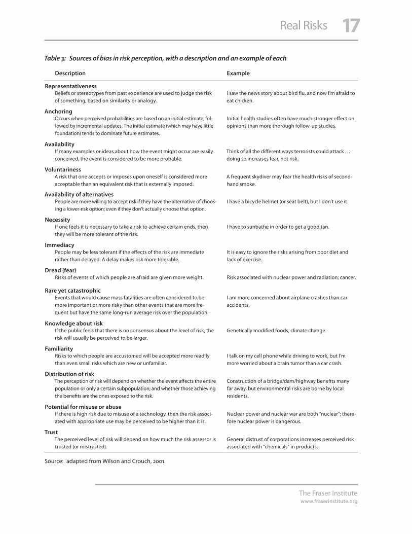
Studies reveal the different ways that risk perceptions are formed; that is, the methods people use to arrive at personal estimates of probability when only partial information is available, and the cognitive shortcuts people use to determine the rela-tive importance of different risks. Interestingly, studies suggest that the actual probabil-ity that an event will occur—the real risk—often plays a negligible role in determining the perceived level of concern [Slovic, Finucane, Peters, and MacGregor, 2004; Margolis 1996]. Instead, what matters are the various characteristics of the risk in question, and the ways these characteristics are processed in a person’s mind. Table 3 (p. 17) summarizes 14 ways in which bias may enter into the perception of a risk.

The generation of nuclear power is a technological example illustrating the gap that can exist between expert risk assessments and public risk perception, and how, once formed, this gap can be extremely difficult to bridge. The consensus among experts in the field is that nuclear power is an extremely safe technology—the risk of harm from serious accidents is extremely small and the safe disposal of nuclear waste poses no significant technical challenges [Cohen, 1990; IAEA, 2003]. Despite these assurances, many people remain extremely resistant to nuclear power. Why? Nuclear power happens to possess many of the characteristics that lead to an elevated percep-tion of risk. The technology has conceptual connections to radiation (and thereby to cancer), and to nuclear weapons; these connections inspire fear, and fear has great power to increase perceived risk. Two high-profile accidents (Three-Mile Island and Chernobyl) suggest the potential for catastrophes—this is another perception-raising characteristic, even though neither accident was catastrophic in terms of their impact on human health [Lieberman, 1997; Jaworowski, 2004]. Nuclear power plants have accu-mulated an outstanding number of accident-free hours and have the strictest safety

17


Real Risks

Table 3: Sources of bias in risk perception, with a description and an example of each

Description Example

RepresentativenessBeliefs or stereotypes from past experience are used to judge the risk of something, based on similarity or analogy.

I saw the news story about bird flu, and now I’m afraid to eat chicken.

AnchoringOccurs when perceived probabilities are based on an initial estimate, fol-lowed by incremental updates. The initial estimate (which may have little foundation) tends to dominate future estimates.

Initial health studies often have much stronger effect on opinions than more thorough follow-up studies.

AvailabilityIf many examples or ideas about how the event might occur are easily conceived, the event is considered to be more probable.

Think of all the different ways terrorists could attack … doing so increases fear, not risk.

VoluntarinessA risk that one accepts or imposes upon oneself is considered more acceptable than an equivalent risk that is externally imposed.

A frequent skydiver may fear the health risks of second-hand smoke.

Availability of alternativesPeople are more willing to accept risk if they have the alternative of choos-ing a lower-risk option; even if they don’t actually choose that option.

I have a bicycle helmet (or seat belt), but I don’t use it.

Necessity If one feels it is necessary to take a risk to achieve certain ends, then they will be more tolerant of the risk.

I have to sunbathe in order to get a good tan.

ImmediacyPeople may be less tolerant if the effects of the risk are immediate rather than delayed. A delay makes risk more tolerable.

It is easy to ignore the risks arising from poor diet and lack of exercise.

Dread (fear)Risks of events of which people are afraid are given more weight. Risk associated with nuclear power and radiation; cancer.

Rare yet catastrophicEvents that would cause mass fatalities are often considered to be more important or more risky than other events that are more fre-quent but have the same long-run average risk over the population.

I am more concerned about airplane crashes than car accidents.

Knowledge about riskIf the public feels that there is no consensus about the level of risk, the risk will usually be perceived to be larger.

Genetically modified foods, climate change.

FamiliarityRisks to which people are accustomed will be accepted more readily than even small risks which are new or unfamiliar.

I talk on my cell phone while driving to work, but I’m more worried about a brain tumor than a car crash.

Distribution of riskThe perception of risk will depend on whether the event affects the entire population or only a certain subpopulation; and whether those achieving the benefits are the ones exposed to the risk.

Construction of a bridge/dam/highway benefits many far away, but environmental risks are borne by local residents.

Potential for misuse or abuseIf there is high risk due to misuse of a technology, then the risk associ-ated with appropriate use may be perceived to be higher than it is.

Nuclear power and nuclear war are both “nuclear”; there-fore nuclear power is dangerous.

TrustThe perceived level of risk will depend on how much the risk assessor is trusted (or mistrusted).

General distrust of corporations increases perceived risk associated with “chemicals” in products.

Source: adapted from Wilson and Crouch, 2001.

18


Real Risks

standards possible, but the industry does not have the full trust of the public, and the physics behind the issues is not well understood by the average person. As a result, the objective evidence has little effect.

The differences between expert assessment and public risk perceptions pose a considerable problem for orderly risk management in society. The differences can go quite deep: even the perception of risk perception varies drastically across different groups. Many risk analysts feel that risk perception simply reflects biases that should be ignored or eliminated—the public needs to be “educated” to come to agreement with the experts. Others view public risk perception as (somehow) more inclusive, broad-based, and forward-thinking than expert assessments [Slovic, 1987]. The truth, of course, will vary between these extremes for different cases.

Institutional and individual perspectives

Problems of risk are usually considered in two stages: risk assessment, where informa-tion about the probability and severity of the risk is gathered; and risk management, where decisions are made about how to act on the risk, taking into consideration other factors such as cost, benefit, alternatives, values, and so on. Significantly, this two-step process may be carried out in entirely different ways by individuals and by the institu-tions of society. The ways in which the institutional and individual perspectives differ, and sometimes conflict, are strongly coloured by the role of risk perception.

Any institution has a generally accepted responsibility to use its resources in an efficient manner, and to act in the best interests of those it represents. Governments and regulatory bodies clearly have responsibility to the public at large, while cor-porations are answerable to their shareholders and (increasingly) bear a general social responsibility as well. In matters of risk, this responsibility forces—or should force—institutions to perform risk assessment and risk management according to some formal, standardized, and defensible process. The appropriate process, and the risk assessment and management principles it should be based on, are the subject of much debate and policy analysis. It is hopefully beyond question, however, that some formalism and accountability is required at the institutional level of risk man-agement. The government that spends millions filling potholes while neglecting to provide clean water to its citizens may be applauded by cyclists but it is not providing efficient risk management.

Risk management at the individual level, by contrast, is carried out in a con-tinuous stream of dozens of small decisions made by each person every day. All of us have at least partial freedom to choose where we live, where we work (and how we get there), what kind of friends we keep, what we eat, and how we spend our spare time. Our decisions, and the habits that develop from them, implicitly define our risk-assessment process and our risk-management values, even if most of us have no formal

19


Real Risks

plan or statement of risk priorities. Personal decisions are based on individual values and on risk perceptions. Perception dominates decision -making for individuals much more than it does for institutions, simply because individuals are real people, with jobs, families, and things to do. They have less time, less information, and less training for performing analysis. While to some extent everyone bases decisons on their percep-tions, the argument made in this report is that individuals should strive to make valid interpretations of the information they have. Beyond this, decision-making depends on personal values.

When the actions and beliefs of institutions differ radically from those of indi-viduals, considerable conflict can arise. Suppose that the public are overwhelmingly concerned about a risk that, like potholes in the previous example, is unimportant in the formal analysis; what should the government do? Can the government use commu-nication, education, and persuasion to convince the public of an alternative action? If such efforts fail, should the government respect the will of the people and start paving or force the alternatives on the unwilling subjects? In the clash between institutional and individual perspectives, risk touches on fundamental questions about the nature of society [Slovic, 1993].

Risks old and new

The final stop in this tour of the risk landscape is a distinction that establishes two dif-ferent groups of risks. Following Wilson and Crouch [2001: 26], risks can be divided into two categories: “historical” risks and “new” risks. The first category, historical risks, is for events or outcomes that are known to occur, can be observed, and occur frequently enough for a significant amount of data to have been collected over the years. It is pos-sible to quantify with reasonable accuracy the danger posed by historical risks. New risks, on the other hand, are either hypothetical, never having been observed, or are observed only rarely. The actual degree of danger associated with a new risk is often highly uncertain.

Note that the terms historical and new do not directly relate to how long we have been aware of a risk, or to how severe or frequent a risk may be. The real basis for putting a risk in one category or the other is the amount of data available. The risks posed by cardiovascular disease or motor-vehicle accidents, for example, are histori-cal—thousands of deaths every year are recorded and unambiguously assigned to each of these causes; the mechanisms through which these events happen are understood and the available data provides a comprehensive summary of the impact they have in society. New risks, on the other hand, may be rare catastrophic events (such as severe global warming, meteor impacts, or full-scale nuclear war) for which there is little or no historical precedent; or they could be low-level, population-wide health impacts that are hypothesized but difficult to observe (such as cancers caused by food additives

20


Real Risks

and household chemicals). In this scheme, a new risk may become a historical risk once more information is gathered, much as the risks associated with cigarette smoking moved from hypothetical to incontrovertible over time.

The distinction between historical and new risks translates into differences in how risks are assessed. For historical risks, the probability that the event occurs may be estimated fairly straightforwardly from past occurrences. The underlying causal mechanism is usually not in question, so that uncertainty in the risk estimate primar-ily reflects variation in the data or problems inherent in the design of the studies. New risks require a more involved process, where the event is broken down into contribut-ing parts and each part is studied mechanistically; at the end, the understanding of the individual parts is combined through a model to predict the behavior of the whole. Throughout this process, there is necessarily more focus on the basic science, more assumptions made, and more debate about the best models to use. A good example of this is the evaluation of the carcinogenic potency of substances. Measurements of the cancer-causing potential of a substance are often done by administering enormous doses of the substance to rats or mice. Applying these results to humans involves two simultaneous extrapolations: jumping the species barrier from rodents to humans, and using results at high doses to predict results at small doses. Determining whether, when, and how these extrapolations may be validly performed is itself an extremely complicated and controversial scientific question [ACSH, 2005]. As a result, carcinoge-nicity as measured by such toxicological studies alone is fraught with uncertainty.

For the information consumer, new risks and historical risks have much in com-mon. Both types of risk will be reported in the news; both will have statistics reported; and both may have slant or bias imposed by the media. Both may be significantly affected by risk perception and cognitive biases. In both cases, the burden is on indi-viduals: to simply accept the message that has been prepared for them or to interpret the information they receive in the larger context of risk, in their lives, and in society.

In the remainder of this publication, the focus will be on historical risks—spe-cifically, historical mortality risks. This is done for two reasons: first, to limit the dis-cussion to a manageable scope; and second, because historical risks summarize those dangers that are known to affect people in the present. As such, the historical mortality risks are an appropriate starting point for gaining more perspective on the nature of risk in everyday life.

Back to statistical thinking

The foregoing review was intended to give some perspective on the multifaceted subject of risk and to help show the place of individuals in the bigger picture of risk in society. Personal intuitions about risk are subject to cognitive biases that can lead to inconsistencies between perceived and real risk levels. The attitudes and

21


Real Risks

decisions of each person have an impact not only on their own health risk but also on the larger issue of how risks are prioritized and managed at the social level.

One of the main reasons to commend statistical thinking is its power to inform individual risk assessment and, thereby, to improve health outcomes on both the indi-vidual and social scale. If opinions take valid interpretation of the data as their starting point, everyone benefits. Valid interpretation requires good thinking about problems, along the following lines.

Poor thinking … tends to be characterized by too little search, by overconfidence in hasty conclusions, and—most importantly—by biases in favor of the possibili-ties that are favored initially. In contrast, good thinking consists of (1) search that is thorough in proportion to the importance of the question, (2) confidence that is appropriate to the amount and quality of thinking done, and (3) fairness to other possibilities than the one we initially favor … Thinking that follows these principles can be called actively open-minded thinking. [Baron, 2000: 191–92]

Whatever one’s opinion on various risks, it is hard to find fault with the concept of actively open-minded thinking as an ideal of clear thought. Statistical thinking, with its focus on process and context, provides a mechanism for actively open-minded thinking when dealing with statistics and chance events.

22


Real Risks

2 An analysis of Canadian mortality data

I detest life-insurance agents. They always argue that I shall someday die, which is not so.

—Stephen Leacock

The time has come to illustrate how each person can use statistical thinking to make risk-related information more meaningful in his or her life. The basic ideas may be illustrated as follows. Suppose you see a news story reporting that ten people in Canada were killed by lightning while playing golf last year. With an assumed 30 million people in Canada, that’s a death rate of one in three million, or about 0.00000033 deaths per person per year. How important is this information to you? That depends. You might first question the validity of the information itself. Is 10 deaths per year typical for this event or was there a rash of lightning strikes in the past year? Did the deaths occur randomly across the country or did nine of them happen at Treeless Acres Golf Club, at the top of beautiful Mount Stormy? You might also consider how the information relates to you in particular. No matter who you are, the average death rate from golf-related lightning-strikes of one in three million is almost certainly meaningless to you. You are at no risk if you never golf; but if you get a thrill out of golfing during thunder-storms, you should consider this carefully. Finally, even if you have reason to worry, it is not clear how much you should worry. Is your lifetime risk of being struck by lightning while playing golf greater than your lifetime risk of being struck while doing something else? How does the risk of dying during your round compare to the risk of dying in a car accident during the half-hour drive to the course? There is no way to put things in perspective if you only know that 10 people died in this manner last year.

This fictitious example illustrates the main questions involved in statistical think-ing about risk: questions about process and context. By what process was the data gener-ated? By what process was it reported? By what processes will I be exposed to this risk? What is the context of variation to which I can compare the given numbers? What is the context of other risks I can compare to the risk in question? In the golf example, the interpretation may seem obvious, even trivial. But for a real set of mortality data, a more conscious effort at statistical thinking is probably required. This is not because the prob-lems are more difficult but because the amount of data is larger and the stakes, higher.

The data set

All deaths in Canada are registered by age and cause, using the World Health Organization’s International Classification of Diseases (ICD) system. The system pro-vides a consistent way to classify mortality data. Comprehensive reporting of ICD

23


Real Risks

codes for deaths enables quantitative comparison of causes of mortality. The mortality data constitutes an up-to-date snapshot of causes of death and should be of primary interest to risk-conscious Canadians.

The ICD system is currently in its tenth revision, ICD-10. It is a hierarchical clas-sification method with thousands of alphanumeric codes, each code corresponding to a disease, condition, or event. Its tree structure begins with highest-level categories for the broadest classes of events; each of these categories has sub-categories for more spe-cific types of events in that class, and so on for several levels of branching. Accidents, for example, constitute codes V01 to X59; transport accidents form a subgroup within this category (V01–V99); injuries to cyclists form a subgroup within transport acci-dents (V10–V19), and so on down to “Pedal cyclist injured in collision with pedestrian or animal, passenger injured” (V11.5). In this way, any study may be done at different levels of detail by choosing an appropriate grouping of the codes.

The discussion below focuses on the Mortality, Summary List of Causes reports issued annually by Statistics Canada [Statistics Canada 2006b, 2006c, 2006d, 2006e, 2007]. These reports provide mortality data based on the ICD codes but arranged into 113 different groupings of causes. The groupings are chosen to have an intermediate level of detail, so that all of the major causes of death (and many minor ones) may be consid-ered, while keeping the number of categories manageable. The 113 groups of causes may be further grouped into a smaller number of categories for convenience—for example, 24 of the 113 causes are malignant neoplasms (cancers), and these categories may be grouped when it is desired to look at only the highest level of information.

Each year’s data comes in the same format. The number of deaths due to each cause are recorded for each of 19 five-year age groups (0–4, 5–9, 10–14, and so on up to the last interval, 90+). The data are also provided separately for each gender but for the majority of this study the numbers for men and women will be combined.

The mortality data from the five years from 2000 to 2004 were aggregated to produce a single data set. This information can be used in combination with census data—population estimates as of July 1 for the same age groups over the same range of years [Statistics Canada, 2004, 2006a]—to estimate the probability of death by differ-ent causes, at any age. The age- and cause-specific probabilities can be further used to calculate life expectancy and other summaries of mortality risk. The mortality data-set can thus be used to inform people of the real risk associated with various causes of death, a starting point for prioritizing risk mitigation for individuals. It is also useful as a vehicle to discuss statistical thinking.

Life expectancy

How long can a person expect to live? One way to approach this question is through the construction of a life table. Life tables are a traditional way for actuaries and

24


Real Risks

demographers to summarize the mortality experience of an entire population at a cer-tain point in time. The so-called ordinary life table (OLT) can be constructed from the mortality data and the census information. The two most important outputs from a life table analysis are the survival function and the life expectancy. [2] These are described below, and shown in table 4.

l The survival function is the fundamental result of a life-table calculation. The value of the survival function at age X gives the probability of living to that age; or, put anoth-er way, it tells us the proportion of people who live to reach age X. For example, the value of the survival function at age 70 is 0.8106, indicating that about 81% of people should live to reach 70 years old.

l The life expectancy column reports the estimated average number of additional years a person will live, as a function of their current age. The single value from an OLT that is commonly used in popular discussion is the life expectancy at birth (age zero). In the case of table 4, this value is 79.8 years.

It may seem surprising that so much information can be gleaned from simple popula-tion estimates and death counts. This surprise is not misplaced: this richness of infor-mation comes at a price.

[2] The OLT is a calculation instrument more than it is an informative display, so only the important results are shown here. The complete OLT is given as table 9, in the Appendix.

Table 4: Life expectancy (years) and survival function in Canada, based on aggregated

mortality data from 2000 to 2004

Age Survival Function

Life Expectancy

Age Survival Function

Life Expectancy

0 1.0000 79.8 50 0.9586 31.8

5 0.9941 75.2 55 0.9416 27.4

10 0.9935 70.3 60 0.9152 23.1

15 0.9928 65.3 65 0.8734 19.1

20 0.9905 60.5 70 0.8106 15.3

25 0.9875 55.6 75 0.7189 12.0

30 0.9847 50.8 80 0.5907 9.0

35 0.9813 46.0 85 0.4261 6.6

40 0.9765 41.2 90 0.2397 4.7

45 0.9695 36.4


25


Real Risks

Check the assumptionsWhen we are presented with quantitative information, such as “the life expectancy in Canada is 79.8 years,’’ there is often a tendency to treat this information as an immu-table fact: the quantity has been measured, it is what it is, and we must accept it. The real situation is rarely so clear, however. Statisticians, actuaries, demographers, medi-cal scientists, and other professionals generally find the world just as confusing as everyone else. These technical professionals differ from the general public mainly in that they are trained in appropriate ways to simplify complex reality into manageable pieces—hopefully with minimal distortion of the truth. Understanding how a given statistic relates to the truth, and how it may deviate from the truth, requires some understanding of the process used to generate the number—in particular, an under-standing of the statistic’s underlying assumptions.

The measurement of life expectancy provides a good example of the importance of assumptions. First, popular reports will usually refer simply to the “life expectancy” (79.8 years in this case). The quoted number is actually the life expectancy at birth; the average adult that has already lived a few decades will not necessarily be expected to live to the same age. The good news is that the expected length of life actually increases as a person gets older. This is because, with every passing year that you survive, you have avoided many risks that could have killed you. The life expectancy column in table 4 reports the number of additional years one can expect to live at various ages, so it is worth considering more than just the first entry in the column. At birth, the table does indeed show 79.8 years; but a 50-year-old can expect 31.8 more years of life, with average age at death increased to 81.8. For those that make it to age 80, the average age at death has increased to 89; it would, after all, be absurd to apply a life expectancy of 79.8 to someone who has already reached age 80.

The indiscriminate use of life expectancy at birth is an example of a common problem in the interpretation of statistics: using the answer without considering the question. When we hear a “life expectancy” number, it is natural to apply this informa-tion to ourselves; however, the life expectancy (at birth) is not an appropriate answer to the question of how long an individual adult can expect to live.

There is a second, and even more serious, problem in applying the results of an ordinary life table to an individual person. The OLT is based upon a critical assumption, called the stationary population assumption: the survival function is assumed to be constant throughout all future time. In other words, it is assumed that the death rates for all ages and for all causes will be the same 100 years from now as they are today. This is fine for the purpose of producing a table; but it is absurd in the real world, where lon-gevity is constantly increasing due to advances in science and technology. So a person in the life table at age 50 may indeed be expected to live to 81.8 years old; but an average real-world 50-year-old will live considerably longer if longevity trends continue.

So what good is the life table? The table is generated from data collected over a short period of time—the years 2000 to 2004 in our case. Though it gives the impression

26


Real Risks

of tracking a set of people over their entire lifetimes, the OLT is actually intended to be a snapshot of the mortality experience of a population at a given point in history. Its best use is as a comparative measure. Through the repeated construction of tables, either across different populations or for a single population over time, one can explore differences or changes in mortality rates. Like all statistical instruments, the life table is perfectly valid if used with open eyes but potentially misleading if accepted blindly. To interpret the information appropriately, readers of table 4 need to ask themselves about the processes behind the numbers: the questions these statistics are intended to answer, the raw data collected to produce the output, and the assumptions involved in going from the raw data to the summary statistics.

No one is averageAverages are the type of statistic most commonly encountered by the public. They provide easily used summaries: average house prices, average investment returns, aver-age temperature and rainfall. By quoting an average, an entire distribution of possible outcomes is distilled into a single number. But it is a statistical truism that an average should not be used without some consideration of the distribution of the underlying data; the context of variation from which the average is constructed is often of critical importance. Hence the stale joke about the statistician who drowned in a river that was only 10 centimetres deep—on average.

The difficulty applying the results of a life table to a particular individual has just been discussed, on the basis of the assumptions involved in the calculations. Even if we agree to swallow the assumptions and treat the table as if it applies to ourselves, we should remember that the life table contains estimated average values, based on the entire population. While there is a sense in which average values apply to everyone, there is another sense in which they apply to no one at all. No one is exactly average: the survival function and life expectancies in table 4 apply to a person that constantly shares the same risk for all diseases as everyone else and who, moreover, is half male and half female. Anyone attempting to interpret what the OLT means to them would do well to consider what makes them unique. The average mortality experience is valid to you only to the extent that you are average—your own health future will be strongly influenced by any special risk factors you have or that characterize the particular sub-population of which you are a member.

Males and females provide two subpopulations that nicely illustrate how aver-age values can overlook important aspects of a situation. The ordinary life table was constructed using aggregate of data for males and females. Separate tables can be constructed for each gender and doing so confirms a result that may be familiar to most readers: females have considerably greater life expectancy than males. Selected information from the gender-specific life tables is given in table 5. It is clear from this table that the life table for the whole population given previously overlooks (or averages out) some important information. The difference in life expectancy between

27


Real Risks

women and men is approximately five years at birth, and remains nearly constant, only dropping to 4.1 years at age 50. The gap slowly decreases at older ages.

If one were only presented with the life table for the whole population, the gen-der difference would not be apparent. This illustrates one key question when presented with an average value: are all the individuals that were included in this average really the same? If the group being averaged contains subpopulations (men and women, in this case), then the average may conceal important information. If the subpopulations are sufficiently different from one another, the average might be inappropriate for describing either group.

The distribution of the dataIt is also vital when considering an average value to question the distribution of the data used to construct the average. The gender-specific life tables can be used to illustrate this question as well. The life expectancies at birth (77.2 for males, 82.2 for females) tell

Table 5: Selected results from ordinary life tables produced separately

for males and females

Age Death rate per 100,000 Life Expectancy

Males Females Males Females

0 129 108 77.2 82.2

5 13 9 72.7 77.6

10 16 12 67.8 72.7

15 64 29 62.8 67.7

20 85 33 58.0 62.8

25 80 34 53.2 57.9

30 93 46 48.4 53.0

35 125 71 43.7 48.1

40 178 108 38.9 43.3

45 278 175 34.2 38.5

50 438 279 29.7 33.8

55 705 437 25.3 29.2

60 1,175 703 21.1 24.8

65 1,890 1,122 17.2 20.6

70 3,075 1,816 13.7 16.7

75 5,058 3,074 10.6 13.0

80 8,312 5,358 7.9 9.8

85 13,969 9,866 5.7 7.0

90 23,945 20,071 4.2 5.0


28


Real Risks

us only that men, on average, live shorter lives than women. They provide no infor-mation on the manner in which mortality experiences differ for males and females. Taking women’s mortality experience as the reference point, there are numerous ways that men might achieve their life expectancy shortfall. Consider several possibilities:

l all men live about 77 years and then die;

l a minority of men die at a young age but the rest of the men live to about 82 years, just like women;

l a larger group of men, though still a minority, die at a young age; those that survive live even longer than the average woman, perhaps dying around age 90.

All of these scenarios could result in a life expectancy gap of five years; but of course the social implications of each scenario are drastically different.

Figure 2 contains information, derived from the life tables, that sheds light on the situation. The figure shows the ratio of the death rate of men to that of women, as a function of age. By indicating how mortality varies with age, this graph conveys a much richer picture than the life expectancies do. The ratio of male death rate to female death rate is always greater than one, indicating that males are at higher risk of dying, on average, throughout their lives. The ratio is surprisingly high—the male

Figure 2: Ratio of male death rate to female death rate, and actual death rate for males, by age


0

1

2

3

0

5,000

10,000

15,000

80706050403020100

Age, X

Rat

io

Dea

ths

per

100

,000

Ratio of male to female death rates (left axis)

Absolute death rate, males (left axis)

29


Real Risks

death rate is over 150% of the female rate from about age 10 to age 75, and reaches a peak of over 250% around age 20. It would seem from this information alone that men, continuously exposed to a much greater risk of dying, should consider themselves lucky to have a reduction of only five years in life expectancy. Why is the gap, then, so small? The second curve in figure 2—showing the absolute death rate—provides the explanation. During the first decades of life, the overall death rates of both males and females are very small. So, although the ratio between male and female death rates may be alarmingly high, comparatively few men actually die in their younger years. Later in life, the ratio is still high but the death rate is much higher. The high ratio over ages 10 to 35 has little effect on the average lifespan, because it accounts for relatively few deaths. So the five-year gap in life expectancy is indeed due primarily to men’s higher mortality in old age.

The distribution of life lengths can be illustrated more directly by comparing the survival functions for men and for women, as done in figure 3. For example, the figure shows that, according to the life table for years 2000–2004—and subject to its assumptions—90% of females and 84% of males are expected to reach age 65; and the chances of living to age 90 are 30% for women and 16% for men. Reporting mor-tality histories as a distribution conveys much more information than just reporting an average.

Figure 3: Survival functions for males and females


Age, X

P (s

urvi

ve to

ag

e X)

Females

Males

0.0

0.1

0.2

0.3

0.4

0.5

0.6

0.7

0.8

0.9

1.0

9080706050403020100

30


Real Risks

Causes of death

The analyses so far have considered only overall mortality, without considering the many different causes of death. The Canadian mortality data breaks down all deaths into 113 ICD-10 codes, however, so that a multiple decrement life table (MDLT) can be constructed. A MDLT essentially splits the ordinary life table into a series of sub-tables, creating estimated survival functions for each cause. These survival functions can be used to calculate many different comparative measures, such as the lifetime probability of dying from a given cause or the life expectancy of a person who eventually dies of a given cause.

The discussion now proceeds into an analysis of different causes of death, using the methods of multiple decrement life tables applied to the Canadian mortality data for 2000 to 2004 (only selected results will be shown; further discussion of the MDLT is given in the Appendix). As with the life expectancy analysis, the results to be pre-sented will be interesting in their own right but the analyses will also illustrate more general issues related to the appropriate interpretation of statistics.

Definitions and measurement systemsThe first duty in studying the different causes of death is to consider the processes used to generate the data at hand. Construction of an MDLT involves the same assumptions as an ordinary life table; in particular, the stationary population assumption (that sur-vival functions remain fixed over time) must be invoked here as well. Accepting this assumption as a necessary evil in order to make progress, we should next question the way in which “cause of death” is defined and measured.

Any statistical summary will contain an implicit statement about definitions and measurement. Why? Because in order to enumerate something—deaths by heart attack, for example—it is necessary to define clear boundaries about what will and will not be counted. Furthermore, the method of counting will play a significant role in determining the accuracy and validity of the result. If an elderly gentleman has a heart attack while water skiing, should this be counted as a heart attack or as a water-sports accident? Regardless of how it should be counted, how will it be counted once the deceased reaches the hospital? Will the reported cause of death for such a case be consistent from site to site and from time to time?

An ideal system for classifying deaths would minimize this sort of problem in two ways: by using an unambiguous set of classification rules and by being perfectly consistent in the application of those rules. The ICD system provides a set of classifica-tion rules but naturally it is difficult to implement the system universally with perfect success. In Canada, death classification happens in two stages. The death certificate is first filled out, usually by a doctor; the certificate is later used by a medical coder to assign a single ICD-10 code. In the report Mortality, Summary List of Causes—2004, Statistics Canada notes:

31


Real Risks

Quality studies done on the certification have shown that approximately one-third of certificates contain major errors. Most of the errors (about 85%) involve the use of non-specific conditions such as “stroke” or “heart failure.” Approximately 10% of the errors involve illogical sequences of conditions entered on the line items. Some of these can be resolved during coding, where the classification rules pinpoint illogical sequences. The remaining 5% involve competing causes. [Statistics Canada, 2007: 130]

This quotation underscores the difficulty of measuring anything, especially social vari-ables, accurately and consistently over the long term and across an entire nation. The statistical thinker is careful to watch for the problems of dubious definitions and erro-neous measurements.

A further conceptual wrinkle related to definitions is the scope of applicability of the mortality data. Note that, when the ICD system is being used to classify deaths by cause, many of the cause-and-effect relationships that might be of interest are out-side the scope of discussion. It is not possible, for example, to use this data set to study the relationship between smoking and lung cancer or to see how many heart attacks are in fact due to water skiing. The “effect” in question is always death and the “causes” under consideration are fixed by the ICD system; the definitions and the measurement system therefore determine the set of questions that the data is capable of answering. This situation is typical: the questions that can be addressed depend on the processes used to collect and analyze the data.

The final process-related topic is the question of the best way to group the 113 causes of death in the data set. To create data summaries for presentation, it is often necessary to reduce the dimension of a data-set to a manageable size by grouping similar information. The particular choices used to define groups can significantly influence how the data is interpreted. The Canadian mortality data are provided as 113 categories but many of these categories are nested within each other as, for example,

“lung cancer” is a sub-category of “cancer.” All of the sub-categories may be grouped into a total of 53 more general categories. Table 6 shows the top 20 causes of death under two scenarios: when the 53 general causes are considered and when the 113 more specific causes are considered. In each scenario, the rankings are based on the lifetime probability of dying from each cause (which can be calculated from the MDLT).

The lists formed using the two grouping methods make many of the same general points—cardiovascular diseases and malignant neoplasms (cancer) are a major feature of both lists—but a closer look reveals considerable differences. Among the 53 general causes, cardiovascular disease and cancer are seen as the dominant causes of death. A wide range of specific diseases are lumped into these two categories, however, effectively letting other more rare diseases enter the top 20. Chronic liver disease and cirrhosis, for example, ranks fourteenth on the more general list. This grouped cause actually consists of two sub-causes: “other chronic liver disease and cirrhosis,” and “alcoholic liver disease.” These two causes rank 43rd and 45th, respectively, out of the 113 more specific causes.

32


Real Risks

Table 6: The top 20 causes of death, when all deaths are first grouped into 53 more general causes (left),

or when all deaths are first grouped into 113 more specific causes (right), ranked by P(death), the lifetime

probability of dying from each cause

More general causes of death More specific causes of deathCause P(death) 1 in … Cause P(death) 1 in …

1 Major cardiovascular diseases 36.49% 2.7 All other forms of chronic ischaemic heart disease

9.91% 10.1

2 Malignant neoplasms 25.66% 3.9 All other diseases (residual) 9.59% 10.4

3 All other diseases (residual) 9.59% 10.4 Acute myocardial infarction 8.72% 11.5

4 Chronic lower respiratory diseases 4.72% 21.2 Cerebrovascular diseases 7.84% 12.8

5 Diabetes mellitus 3.36% 29.8 Malignant neoplasms of trachea, bronchus and lung

6.41% 15.6

6 Accidents (unintentional injuries) 3.28% 30.5 Other chronic lower respiratory diseases

4.19% 23.9

7 Alzheimer’s disease 3.07% 32.6 All other and unspecified malignant neoplasms

3.65% 27.4

8 Influenza and pneumonia 2.82% 35.5 Diabetes mellitus 3.36% 29.8

9 Nephritis, nephrotic syndrome and nephrosis

1.69% 59.0 All other forms of heart disease 3.18% 31.5

10 Symptoms, signs and abnormal clinical and laboratory findings, not elsewhere classified

1.25% 79.8 Alzheimer’s disease 3.07% 32.6

11 Other diseases of respiratory system 0.99% 100.9 Malignant neoplasms of colon, rectum and anus

2.86% 35.0

12 Intentional self-harm (suicide) 0.89% 112.3 Pneumonia 2.66% 37.7

13 Parkinson’s disease 0.80% 124.4 Heart failure 2.59% 38.6

14 Chronic liver disease and cirrhosis 0.75% 132.8 Malignant neoplasm of breast 1.91% 52.5

15 Septicaemia 0.69% 145.5 Malignant neoplasm of prostate 1.73% 57.8

16 In situ neoplasms, benign neoplasms and neoplasms of uncertain or unknown behaviour

0.64% 156.2 Renal failure 1.66% 60.1

17 Pneumonitis due to solids and liquids 0.48% 206.4 Malignant neoplasm of pancreas 1.32% 75.7

18 Certain conditions originating in the perinatal period

0.27% 365.4 Symptoms, signs and abnormal clinical and laboratory findings, not elsewhere classified

1.25% 79.8

19 Anaemias 0.26% 384.7 Other and unspecified nontransport accidents and their sequelae

1.16% 85.9

20 Certain other intestinal infections 0.26% 389.3 Other diseases of respiratory system

0.99% 100.9


33


Real Risks

The top 20 killers by low-level grouping force us to look beyond the catch-all names of cardiovascular disease and cancer, to note that the roster of possible causes of death is truly diverse. The top two causes in this list, “all other forms of chronic ischaemic heart disease” and “all other diseases (residual),” are themselves convenience groupings used to hold numerous rare diseases. This list indicates that if we choose to look at specific causes of death, then we will not have the comfort of worrying about only one or two causes. It also underscores the fact that we live in a world of compet-ing risks; eliminating any one source of risk will not necessarily have a large effect on population mortality.

Which of the two options presented in table 6 is correct? Both are correct: as usual, the better one to use will depend on the particular goals of the reader. Either one can be used incorrectly, however, if no consideration is given to how the causes are grouped. The challenge for the statistical thinker comes when only one of these two top-20 lists is presented. When we see one list, we should ask ourselves what the other list might look like.

Beware of isolated statisticsMany of the illustrations discussed so far have involved looking at the same data in dif-ferent ways, to get a fuller picture of the truth. Developing a habit of doing this is a key step toward statistical thinking. Statistical thinkers actively seek out the information required to put the data they are confronted with into context. If no such information is available, the statistical thinker will know what questions to ask and what mental caveats to retain.

In the mortality data, one of the most important factors that is not visible in the usual statistics is the effect of age. Most of the summaries given so far are either life-time probabilities, overall averages, or values applicable to a single age. As with most published statistics, this was done for the author’s convenience, not for the reader’s. For people to interpret the mortality data as it applies to them, the age effect is essen-tial to provide context. To illustrate how mortality risks from various causes change with age, survival functions were estimated (using the MDLT method) for six broad groups of causes:

1 major cardiovascular diseases; 2 cancer; 3 high-profile diseases (diabetes, Alzheimer’s disease, Parkinson’s disease, HIV); 4 all other diseases; 5 accidents; 6 suicide, homicide, and other events.

A detailed list of these groupings is given in the Appendix. The survival functions for the six causes were used to produce the summary displays in Table 7 and Figure 4.

34


Real Risks

Table 7 shows the probability of dying in the next five years from each of the six causes, for individuals of age 25 and age 65. At 25 years old, the top killers are accidents; suicide and homicide; and all other diseases. In keeping with the good health of youth, the large-scale overall causes of death (cancer, cardiovascular disease, and the high-profile diseases) are actually the least of the young person’s worries. The situation shifts by age 65, however: cancer, cardiovascular disease, and other diseases are at the top of the list. The risk of suicide or homicide remains relatively constant throughout adult-hood, so that it is no longer a significant contributor to mortality at age 65. Interestingly, the high-profile diseases, despite their high profile, are only moderate contributors to overall mortality at age 65. This group of causes is about one sixth as likely as cardiovas-cular disease, and only about twice as likely as accidents, to cause death.

Figure 4 shows the age effect in a different fashion. Rather than looking at a short time horizon of five years, the figure plots the probability of eventually dying from each cause, as a function of the person’s present age. To use the graph, one should read upward from a chosen age value; the heights of the lines associated with each cause give the probability of dying from that cause in the remaining years of life. The sum of the probabilities equals exactly 1 for any age, since everyone must die eventually. This again illustrates the competing nature of risk—when the probability of eventually dying from one cause drops, the probability of dying from some other cause must rise to compensate.

The probabilities in Figure 4 remain roughly constant until about age 50, because few people die in the first decades of life. Cardiovascular disease leads the way during this period with a probability of about 0.37, with cancer and other diseases also above the 0.25 mark; the other causes are relatively much smaller. As age moves into the six-ties, seventies, and beyond, the probability of dying of cancer during one’s remaining lifetime goes down quite sharply, while the risk of death from cardiovascular disease and other diseases increases considerably.

Table 7: Probability of dying from different causes in the next five years,

for persons at age 25 and 65P(die within 5 years)

Age 25 Age 65

Cardiovascular diseases 0.016% 2.0%

Cancer 0.031% 3.3%

High-profile diseases 0.0056% 0.34%

All other diseases 0.054% 1.4%

Accidents 0.093% 0.14%

Suicide, homicide, and other events 0.086% 0.070%

Total (all causes) 0.29% 7.2%


35


Real Risks

Table 7 and Figure 4 help to reveal the effect of age but they also aid a com-parison between the relative magnitude of different risks. Performing such relative comparisons is a vital step when considering risk. Any statistic presented in isolation, without a frame of reference, is of limited value. Consider the following true state-ment: 16,490 deaths in Canada were attributed to renal failure in the years 2000 to 2004. This surely seems like a large number. But, how large is it? Once we learn that it is similar to the number of deaths due to pancreatic cancer (16,505) and that it is in the same ballpark as suicide (18,326) and motor-vehicle accidents (13,910), we can put the information in better context. Even so, it would still be worthwhile to ask what the risk of renal failure is at different ages, what the risk factors are for renal failure, how this information compares to the other comparable risks, and so on.

Figure 4: Probability of eventually dying from different causes, as a function of age


Age, X

P (e

vent

ually

die

from

cau

se k

)

Cardiovascular disease

0.00

0.05

0.10

0.15

0.20

0.25

0.30

0.35

0.40

0.45

0.50

9080706050403020100

All other diseases

High-profile diseases

Accidents

Suicide, homicide, & other

Cancer

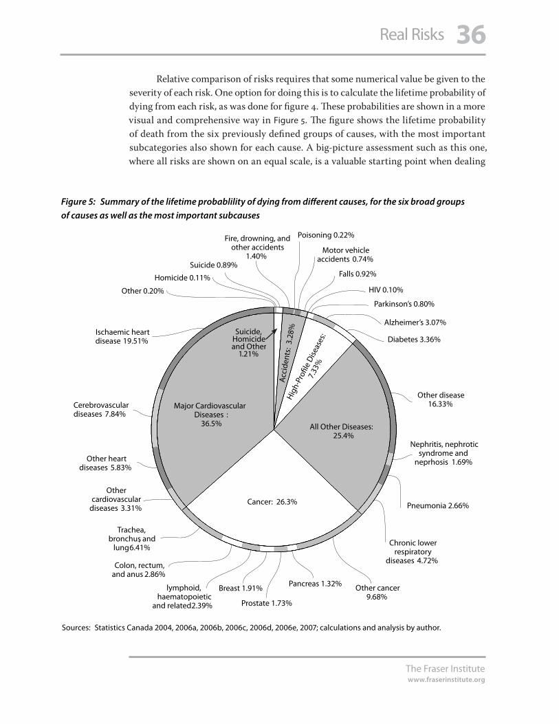
36


Real Risks

Relative comparison of risks requires that some numerical value be given to the severity of each risk. One option for doing this is to calculate the lifetime probability of dying from each risk, as was done for figure 4. These probabilities are shown in a more visual and comprehensive way in Figure 5. The figure shows the lifetime probability of death from the six previously defined groups of causes, with the most important subcategories also shown for each cause. A big-picture assessment such as this one, where all risks are shown on an equal scale, is a valuable starting point when dealing

Figure 5: Summary of the lifetime probablility of dying from different causes, for the six broad groups

of causes as well as the most important subcauses


Ischaemic heart disease 19.51%

Cerebrovascular diseases 7.84%

Other heart diseases 5.83%

Other cardiovascular

diseases 3.31%

Colon, rectum, and anus 2.86%

Trachea, bronchus, and

lung 6.41%

lymphoid, haematopoietic

and related 2.39%

Breast 1.91%

Prostate 1.73%

Other cancer 9.68%

Chronic lower respiratory

diseases 4.72%

Pneumonia 2.66%

Nephritis, nephrotic syndrome and

neprhosis 1.69%

Other disease 16.33%

Diabetes 3.36%

Alzheimer’s 3.07%

Parkinson’s 0.80%

HIV 0.10%

Falls 0.92%

Motor vehicle accidents 0.74%

Poisoning 0.22%Fire, drowning, and other accidents

1.40%

Homicide 0.11%

Other 0.20%

Suicide 0.89%

Major Cardiovascular Diseases :

36.5% All Other Diseases:25.4%

Cancer: 26.3%

Hig

h-Pr

ofile

Dise

ases

:

7.33

%

Acc

iden

ts:

3.28

%Suicide, Homicide and Other

1.21%

Pancreas 1.32%

37


Real Risks

with any specific risk. The risks in the graph all sum to 100%, so we can be sure we are considering each particular risk in the widest possible scope. The relative importance of each risk is immediately called to attention. When viewed in this perspective, it is possible to begin to assess whether priorities (at either the personal or societal level) are in line with the real risks faced throughout life. Without this vital context, we are left making risk decisions based on perception alone.

Is figure 5 the last word in relative risk comparisons? Hopefully it is clear, from everything discussed so far, that there is no last word when it comes to statistical sum-maries. In the case of figure 5, the data provides a formal and accurate way of compar-ing the magnitude of different mortality risks; and it is a valid representation of the mortality experience of the population for the years 2000 to 2004. But a figure such as this also invites over-interpretation; it is potentially misleading in several ways.

1 It may give the impression that, for example, 36.5% of Canadians alive today will die of cardiovascular diseases. This is only true if the (unlikely) stationary population assumption holds.

2 It suggests prioritization of risks based only on overall mortality. Other factors, such as whether a certain cause primarily affects young people, might also be considered important.

3 It ignores the effect of age. The relative importance of different causes varies continu-ously with age but the figure masks this fact.

4 It cannot communicate the comforting truth that survival (not dying) is overwhelm-ingly the most likely outcome for people of any age, over a short time horizon such as a year or five years.

5 It is based on combined data for males and females. As a result, the numbers for dis-eases such as breast cancer or prostate cancer are meaningful only at the population (not the individual) level.

6 It only considers death, not illness. So diseases that are common, but less often fatal, may not be given their due importance from this plot alone.

These problematic points neither invalidate the graph nor render it useless. But they illus-trate a point: every statistic is valid within its boundaries of appropriate use, and danger-ous elsewhere. The role of statistical thinking is to make the boundaries more visible.

38


Real Risks

Conclusion

Many highly intelligent people are poor thinkers. Many people of average intelligence are skilled thinkers. The power of the car is separate from the way it is driven.

—Edward DeBono

Although this report has been ostensibly about risk, its real purpose was to introduce the concept of statistical thinking. Statistical thinking has been proposed as a para-digm for clear thinking in the face of variability and uncertainty. So what is statisti-cal thinking, and how can it be practiced? Statistical thinking has been defined as having two principal aspects: understanding the processes active in a given situation and putting information in an appropriate context. Being mindful of these two basic questions—What is the process? What is the context?—should make it easier to build up statistical thinking skills in various situations.

Process-oriented thinking leads a person to view all the world as a series of interconnected processes. In part 1, we saw how decision-making about risk at the social level is the result of a complex process of interactions between the public and its institutions. We saw how at the individual level, perceptions of risk depend on the cognitive processes we use to relate to information. In part 2, it was shown how appro-priate interpretation of results depends critically on the processes of data collection and data analysis: definitions, measurement systems, assumptions, and models.

In an ideal world, journalists would report more process-related informa-tion in the stories they cover, since a clear understanding of the issues is impossible otherwise. Unfortunately, the media typically report too little about the processes behind the headlines. For example, regarding new or hypothetical health risks, that often hinge on new science, it was concluded: “The procedural and methodologi-cal components of scientific research—which often determine the conclusions, and always shape them decisively—tend to be downplayed if not altogether ignored in news accounts that concentrate on a study’s substantive conclusions” [Murray et al.,

2002: 117]. When it comes to reporting on health and risks, the primary focus is on the conclusions, with little or no concern for how valid they might be or what limitations might exist on their application. The burden of proper interpretation is largely borne by the information consumer.

An awareness of context is the second important ingredient in developing statistical thinking. Analysis of the Canadian mortality data illustrated how useful the search for context can be when applied to questions of risk. Average population values such as life expectancy, for example, were shown to have less significance for an individual than first impression might suggest; the interpretation of the aver-age values depends on contextual information such as individual risk factors or the distribution of individual lifetimes. Consideration of context also brought up the

39


Real Risks

important idea of competing risks. Throughout their lives, all people are exposed to numerous risks simultaneously and acting to change exposure to one risk will undoubtedly affect the level of exposure to other risks as well.

Consideration of context leads from competing risks to the vital idea that risks are relative quantities. To be understood well, risks should not be considered in isola-tion; they should be considered in the context of other risks. In fact, as the analysis of the Canadian mortality data showed, it might not even be sufficient to compare risks only in one way; looking at the comparison from several different angles gives a much clearer picture. The relativity of risks is another idea that the media, in its focus on specific conclusions, often downplays or completely ignores:

We cannot minimize our risks by simply avoiding those we happen to think about … The problem with such an approach is that the risks we think about are those most publicized by the media, whose coverage is a very poor guide to actual dangers. The logical procedure for minimizing risks is to quantify all risks and then choose those that are smaller in preference to those that are larger. [Cohen 1990: 118]

Clearly, just as the process background is often absent, consumers should expect that the appropriate context for interpretation of risk will be absent as well. The consumer needs to use statistical thinking to recognize that vital information is often missing.

Statistical thinking is good thinking in the face of variability and uncertainty, and good thinking is essential for the modern consumer of risk information. Developing statistical thinking skills takes some experience and practice but, once the habits of thought are in place, a person can become much more resistant to misinformation. Risk perception will continue to be determined by values, fears, and other influences—some rational, some irrational. By questioning the processes and by putting informa-tion into context, one can ensure that the already capricious nature of risk perception is not amplified by a misinterpretation of the facts.

40


Real Risks

Appendix: Methodological Notes

The analyses in Part 2 of this publication were all made using methods for abridged life tables. The calculation of the ordinary life table (OLT) and of the multiple decrement life table (MDLT) were as described in the text Survival Models and Data Analysis, sections 4.9 and 10.5 [Elandt-Johnson and Johnson, 1980]. An equivalent, more recent ref-erence is Biostatistical Methods in Epidemiology, chapter 13 [Newman, 2001]. A thorough mathematical and conceptual description of life-table methods is beyond the scope of this publication. Only selected calculations and results are presented below; the reader is directed to the references for more details.

As discussed in the text, the data analyzed were cause-grouped death counts for Canada, years 2000 to 2004. To create the life tables, population estimates as of July 1 for each year were also used. These were obtained from Statistics Canada’s demo-graphic reports from 2003 and 2005 [Statistics Canada, 2004, 2006a]. The 2001 and 2002 data were final postcensal estimates; the 2003 and 2004 data were revised postcensal estimates; and the 2000 data was the final intercensal estimate.

List of causes of death

The 113 lowest-level (more specific) causes used to classify deaths are given in table 8. Each cause is shown with its corresponding ICD-10 codes. The causes are grouped into the six overall categories shown in Table 7, Figure 4, and Figure 5.

Table 8: List of causes—multiple decrement life table (MDLT) groupings

1 Cancer (neoplasms)

of lip, oral cavity and pharynx (C00-C14)

of oesophagus (C15)

of stomach (C16)

of colon, rectum and anus (C18-C21)

of liver and intrahepatic bile ducts (C22)

of pancreas (C25)

of larynx (C32)

of trachea, bronchus and lung (C33-C34)

of skin (C43)

of breast (C50)

of cervix uteri (C53)

41


Real Risks

of corpus uteri and uterus, part unspecified (C54-C55)

of ovary (C56)

of prostate (C61)

of kidney and renal pelvis (C64-C65)

of bladder (C67)

of meninges, brain and other parts of central nervous system (C70-C72)

Hodgkin’s disease (C81)

Non-Hodgkin’s lymphoma (C82-C85)

Leukaemia (C91-C95)

Multiple myeloma and immunoproliferative neoplasms (C88, C90)

Other and unspecified malignant neoplasms of lymphoid, haematopoietic and related tissue (C96)

All other and unspecified malignant neoplasms (various codes)

In situ neoplasms, benign neoplasms and neoplasms of uncertain or unknown behaviour (D00-D48)

2 Cardiovascular Disease

Acute rheumatic fever and chronic rheumatic heart diseases (I00-I09)

Hypertensive heart disease (I11)

Hypertensive heart and renal disease (I13)

Acute myocardial infarction (I21-I22)

Other acute ischaemic heart diseases (I24)

Atherosclerotic cardiovascular disease, so described (I25.0)

All other forms of chronic ischaemic heart disease (I20, I25.1-I25.9)

Acute and subacute endocarditis (I33)

Diseases of pericardium and acute myocarditis (I30-I31, I40)

Heart failure (I50)

All other forms of heart disease (various codes)

Essential (primary) hypertension and hypertensive renal disease (I10, I12)

Cerebrovascular diseases (I60-I69)

Atherosclerosis (I70)

Aortic aneurysm and dissection (I71)

Other diseases of arteries, arterioles and capillaries (I72-I78)

3 High-profile diseases

Human immunodeficiency virus [HIV] disease (B20-B24)

Diabetes mellitus (E10-E14)

Parkinson’s disease (G20-G21)

Alzheimer’s disease (G30)

Table 8 (continued): List of causes—multiple decrement life table (MDLT) groupings

1 Cancer (neoplasms) (continued)

42


Real Risks

4 Accidents

Motor vehicle accidents (various codes)

Other land transport accidents (various codes)

Water, air and space, and other and unspecified transport accidents and their sequelae (V90-V99, Y85)

Falls (W00-W19)

Accidental discharge of firearms (W32-W34)

Accidental drowning and submersion (W65-W74)

Accidental exposure to smoke, fire and flames (X00-X09)

Accidental poisoning and exposure to noxious substances (X40-X49)

Other and unspecified nontransport accidents and their sequelae (various codes)

5 Suicide, homicide, and other events

Suicide by discharge of firearms (X72-X74)

Suicide by other and unspecified means and their sequelae (various codes)

Homicide by discharge of firearms (X93-X95)

Homicide by other and unspecified means and their sequelae (various codes)

Discharge of firearms, undetermined intent (Y22-Y24)

Other and unspecified events of undetermined intent and their sequelae (various codes)

Operations of war and their sequelae (Y36, Y89.1)

Legal intervention (Y35, Y89.0)

Complications of medical and surgical care (Y40-Y84, Y88)

6 All other diseases

Whooping cough (A37)

Scarlet fever and erysipelas (A38, A46)

Meningococcal infection (A39)

Septicaemia (A40-A41)

Syphilis (A50-A53)

Acute poliomyelitis (A80)

Arthropod-borne viral encephalitis (A83-A84, A85.2)

Measles (B05)

Viral hepatitis (B15-B19)

Malaria (B50-B54)

Other and unspecified infectious and parasitic diseases and their sequelae (various codes)

Anaemias (D50-D64)

Malnutrition (E40-E46)

Other nutritional deficiencies (E50-E64)

Meningitis (G00, G03)

Other disorders of circulatory system (I80-I99)


43


Real Risks

Influenza (J10-J11)

Pneumonia (J12-J18)

Acute bronchitis and bronchiolitis (J20-J21)

Unspecified acute lower respiratory infection (J22)

Bronchitis, chronic and unspecified (J40-J42)

Emphysema (J43)

Asthma (J45-J46)

Other chronic lower respiratory diseases (J44, J47)

Pneumoconioses and chemical effects (J60-J66, J68)

Pneumonitis due to solids and liquids (J69)

Other diseases of respiratory system (various codes)

Peptic ulcer (K25-K28)

Diseases of appendix (K35-K38)

Hernia (K40-K46)

Alcoholic liver disease (K70)

Other chronic liver disease and cirrhosis (K73-K74)

Cholelithiasis and other disorders of gallbladder (K80-K82)

Acute and rapidly progressive nephritic and nephrotic syndrome (N00-N01, N04)

Chronic glomerulonephritis, nephritis and nephropathy not specified as acute or chronic, and renal sclerosis unspecified (various codes)

Renal failure (N17-N19)

Other disorders of kidney (N25, N27)

Infections of kidney (N10-N12, N13.6, N15.1)

Hyperplasia of prostate (N40)

Inflammatory diseases of female pelvic organs (N70-N76)

Pregnancy with abortive outcome (O00-O07)

Other complications of pregnancy, childbirth and the puerperium (O10-O99)

Certain conditions originating in the perinatal period (P00-P96)

Congenital malformations, deformations and chromosomal abnormalities (Q00-Q99)

Symptoms, signs and abnormal clinical and laboratory findings, not elsewhere classified (R00-R99)

All other diseases (residual) (various codes)

Sources: Statistics Canada, 2006b; grouped by author.


6 All other diseases (continued)

44


Real Risks

Ordinary life table

Table 9 (p. 46) shows a complete ordinary life table (OLT). Each column is described below.

Age, x

This column specifies the age intervals into which the population is divided. In this study, five-year age intervals were used. The first row (x = 0), for example, contains information about people in the first five years of life: from age 0 up to just before the fifth birthday. The second row covers the age interval from the fifth birthday until just before the tenth birthday, and so on. The last interval is the only exception—it covers the open interval of all ages 90 and above.

Total population at risk, nKx.

Input column. This column contains the population count as of July 1 for each age range, from census data. The values shown are sums over the years 2000 to 2004. Midyear population estimates are used as an estimate of the total population at risk—note they are only estimates, since the exact number of people in any age range is constantly changing due to births, deaths, and birthdays.

Total deaths, nDx

Input column. The number of deaths observed in each age range over the years in ques-tion (2000–2004).

Death rate per 100,000, nMx

Calculated column. For each age range, the death rate is calculated as the observed num-ber of deaths per 100,000 people per year, using the population estimates as of July 1.

Conditional death probability, nqx

Calculated column. The conditional probability is the estimated probability that a per-son of exact age x will die before reaching the exact age x + 5. The conditional probabil-ity for the last age group (90+) is set to 1 by definition. This column is the fundamental column of the life table, on which all of the remaining columns depend. For this table, it was calculated assuming that those who die in a given age interval live, on average, to the halfway point of the interval.

Hypothetical cohort size, lx

Calculated column. This column shows the expected size of a “hypothetical cohort,” usually 100,000 people, all born at the same instant, if the conditional death prob-abilities are applied to them as they get older (i.e., moving down the rows of the table). Note that if we divide this column by 100,000, we get the estimated survival function, which is a more modern and generally useful concept.

45


Real Risks

Number of deaths, ndx

Calculated column. This is the expected number of deaths in the hypothetical cohort as it ages from age x to x + 5.

Person-years lived in the period, nLx

Calculated column. This column contains an estimate of the total number of years lived, by all people in the hypothetical cohort, during the selected five-year interval. This column also assumes that those who die, live 2.5 years into the interval, on average. It is an intermediate step toward calculating the total future years lived.

Total future years lived, Tx

Calculated column. The expected total number of years to be lived, by all people in the cohort, during the present age interval and all subsequent age intervals. It is used in calculation of life expectancy.

Life expectancy, ex

The average number of additional years to be lived: the total future years lived divided by the present cohort size.

Survival functionAs mentioned in the text, life tables are traditional calculation instruments, and so most of the columns in them are not particularly enlightening. The OLT is structured toward the calculation of life expectancies. The important point for the average reader, however, is that death counts and demographic statistics can be combined to estimate the survival function—the probability of living to a given age. Once the survival func-tion has been estimated, other quantities like the life expectancy, or the chance of dying in a given time interval, can be calculated using standard methods.

Multiple decrement life table The multiple decrement life table (MDLT) is actually a series of ordinary life tables, one constructed for each cause of interest. The only difference between construction of an MDLT and an OLT is in the way the conditional death probabilities are obtained. For each age group, the overall conditional probability (from the OLT) is partitioned among all of the selected causes in proportion to the number of deaths attributed to each cause. Once these cause-specific conditional probabilities are established, the OLT columns, described above, are all calculated separately for each cause; the result is an MDLT. The MDLT contains survival functions for each particular cause; these survival functions can be used (along with the overall survival function) to calculate useful quantities such as the lifetime probability of dying from a particular cause.

46


Real Risks

Table 9: Ordinary life table, Canada, 2000–2004, males and females combined

Age Total population

at risk

Total deaths Death rate per 100,000

Conditional death

probability

Hypothetical cohort size

Number deaths

Person-years lived in period

Total future years lived

Life expectancy

x nKx nDx nMx nqx lx ndx nLx Tx ex

0 8,694,038 10,335 119 0.00593 100,000 593 498,518 7,976,326 79.8

5 9,915,149 1,129 11 0.00057 99,407 57 496,895 7,477,808 75.2

10 10,481,518 1,501 14 0.00072 99,351 71 496,576 6,980,912 70.3

15 10,591,592 4,979 47 0.00235 99,280 233 495,816 6,484,336 65.3

20 10,746,090 6,424 60 0.00298 99,047 296 494,494 5,988,520 60.5

25 10,529,308 6,026 57 0.00286 98,751 282 493,050 5,494,026 55.6

30 11,197,726 7,813 70 0.00348 98,469 343 491,487 5,000,977 50.8

35 12,796,912 12,530 98 0.00488 98,126 479 489,431 4,509,490 46.0

40 13,418,723 19,159 143 0.00711 97,647 695 486,497 4,020,058 41.2

45 12,232,130 27,682 226 0.01125 96,952 1,091 482,033 3,533,561 36.4

50 10,713,354 38,355 358 0.01774 95,861 1,701 475,054 3,051,528 31.8

55 8,700,434 49,570 570 0.02809 94,160 2,645 464,191 2,576,474 27.4

60 6,731,490 62,892 934 0.04565 91,516 4,178 447,135 2,112,283 23.1

65 5,745,807 85,699 1,492 0.07189 87,338 6,279 420,993 1,665,148 19.1

70 5,143,295 123,387 2,399 0.11316 81,059 9,173 382,363 1,244,155 15.3

75 4,143,866 162,227 3,915 0.17829 71,886 12,817 327,389 861,792 12.0

80 2,767,207 179,163 6,475 0.27863 59,069 16,458 254,201 534,403 9.0

85 1,456,929 163,206 11,202 0.43756 42,611 18,645 166,443 280,202 6.6

90 720,818 151,858 21,067 1.00000 23,966 23,966 113,759 113,759 4.7


47


Real Risks

References

American Council on Science and Health [ACSH] (2005). America’s War on “Carcinogens”: Reassessing the Use of Animal Tests to Predict Human Cancer Risk. American Council on Science and Health.

Balestracci, Davis (1998). Data “Sanity”: Statistical Thinking Applied to Everyday Data. Special Publication, Summer 1998. ASQ Statistics Division.

Baron, Jonathan (2000). Thinking and Deciding. Third ed. Cambridge University Press.

Britz, Galen, Donald Emerling, Lynne Hare, Roger Hoerl, and Janice Shade (1996). Statistical Thinking. Special Publication, Summer 1998. ASQ Statistics Division.

Cohen, Bernard L. (1990). The Nuclear Energy Option: An Alternative for the 90s. Plenum Press.

Campbell, Stephen K. (1974/2004). Flaws and Fallacies in Statistical Thinking. Reprint. Dover Publications.

Elandt-Johnson, Regina C., and Norman L. Johnson (1980). Survival Models and Data Analysis. John Wiley & Sons.

International Atomic Energy Agency [IAEA] (2003). The Long Term Storage of Radioactive Waste: Safety and Sustainability. International Atomic Energy Agency.

Jaworowski, Zbigniew (2004). Radiation Folly. In Kendra Okonski and Julian Morris (eds.), Environment and Health: Myths and Realities (International Policy Press): 68–86.

Kasperson, Roger E., Ortwin Renn, Paul Slovic, Halina S. Brown, Jacque Emel, Robert Goble, Jeanne X. Kasperson, and Samuel Ratick (1988). The Social Amplification of Risk: A Conceptual Framework. Risk Analysis 8, 2: 177-87.

Lieberman, Adam J. (1997). Facts versus Fears: A Review of the Greatest Unfounded Health Scares of Recent Times. Third ed. American Council on Science and Health.

Margolis, Howard (1996). Dealing with Risk: Why the Public and the Experts Disagree on Environmental Issues. University of Chicago Press.

48


Real Risks

Murray, David, Joel Schwartz, and S. Robert Lichter (2002). It Ain’t Necessarily So: How the Media Remake Our Picture of Reality. Penguin Books.

Newman, Stephen C. (2001). Biostatistical Methods in Epidemiology. John Wiley & Sons.

Piattelli-Palmarini, Massimo (1994). Inevitable Illusions: How Mistakes of Reason Rule Our Minds. John Wiley & Sons.

Shachter, Ross D. (1986). Evaluating Influence Diagrams. Operations Research 34, 6: 871–82.

Slovic, Paul (1987). Perception of Risk. Science 236: 280–85.

Slovic, Paul (1993). Perceived Risk, Trust, and Democracy. Risk Analysis 13, 6: 675–82.

Slovic, Paul, Melissa L. Finucane, Ellen Peters, and Donald G. MacGregor (2004). Risk as Analysis and Risk as Feelings: Some Thoughts about Affect, Reason, Risk, and Rationality. Risk Analysis 24, 2: 311–22.

Statistics Canada (2004). Annual Demographic Statistics, 2003. Catalogue no. 91-213-XIB. Statistics Canada.

Statistics Canada (2006a). Annual Demographic Statistics, 2005. Catalogue no. 91-213-XIB. Statistics Canada.

Statistics Canada (2006b). Mortality, Summary List of Causes: 2000. Catalogue no. 84F0209XIE. Statistics Canada.

Statistics Canada (2006c). Mortality, Summary List of Causes: 2001. Catalogue no. 84F0209XIE. Statistics Canada.

Statistics Canada (2006d). Mortality, Summary List of Causes: 2002. Catalogue no. 84F0209XIE. Statistics Canada.

Statistics Canada (2006e). Mortality, Summary List of Causes: 2003. Catalogue no. 84F0209XIE. Statistics Canada.

Statistics Canada (2007). Mortality, Summary List of Causes: 2004. Catalogue no. 84F0209XIE2004000. Statistics Canada.

49


Real Risks

Tversky, Amos, and Daniel Kahneman (1974). Judgment Under Uncertainty: Heuristics and Biases. Science 185: 1124–31.

Wild, C. J., and M. Phannkuch (1999). Statistical Thinking in Empirical Enquiry. International Statistical Review 67, 3: 223–65.

Wilson, Richard, and Edmund A. C. Crouch (2001). Risk-Benefit Analysis. Second ed. Harvard University Press.

50


Real Risks

About the author

Mark Wolters

Mark Wolters is a professional engineer originally from Vernon, British Columbia. His enthusiasm for statistical thinking led him to quit his job as a senior fuel-cell engineer and study statistics full time. He has recently completed his master’s degree at Simon Fraser University and is currently pursuing a doctorate in the Department of Statistical and Actuarial Sciences at the University of Western Ontario.

Acknowledgments

The author and the Risk & Environment Centre of The Fraser Institute would like to thank the generous supporters of The Fraser Institute who funded this project. We would also like to thank Andy Torr for his editorial assistance; and Carolyn Huston (Department of Statistics, Simon Fraser University), Kenneth P. Green (Resident Scholar, American Enterprise Institute), Angela Logomasini (Director of Risk and Environmental Policy, Competitive Enterprise Institute), and Fred McMahon (Director of Centre for Globalization Studies, The Fraser Institute), who reviewed and made suggestions for improving this publication. Any remaining errors or omissions are the sole responsibility of the author. As the author of this publication has worked inde-pendently, opinions expressed by him are his own and do not necessarily reflect the opinions of the supporters, trustees, or other staff of The Fraser Institute. This publica-tion in no way implies that The Fraser Institute, its trustees, or staff are in favor of, or oppose the passage of, any bill.

51


Real Risks

Publishing information

Fraser Institute Digital Publications are published from time to time by The Fraser Institute to provide, in a format easily accessible on-line, timely and comprehensive studies of current issues in economics and public policy.

DistributionThese publications are available from <http://www.fraserinstitute.ca> in Portable Document Format (PDF) and can be read with Adobe Acrobat® or with Adobe Reader®, which is available free of charge from Adobe Systems Inc. To down-load Adobe Reader, go to this link: <http://www.adobe.com/products/acrobat/readstep2.html> with your Browser. We encourage you to install the most recent version.

Ordering publicationsFor information about ordering the printed publications of The Fraser Institute, please contact the publications coordinator

l e-mail: [email protected] l telephone: 604.688.0221 ext. 580 or, toll free, 1.800.665.3558 ext. 580 l fax: 604.688.8539.

MediaFor media enquiries, please contact our Communications Department

l telephone: 604.714.4582 l e-mail: [email protected].

CopyrightCopyright© 2007 by The Fraser Institute. All rights reserved. No part of this publica-tion may be reproduced in any manner whatsoever without written permission except in the case of brief passages quoted in critical articles and reviews.

ISSN1714–6739

Date of issueDecember 2007

Editing, design, and productionLindsey Thomas Martin & Kim Forrest

http://www.fraserinstitute.ca

http://www.adobe.com/products/acrobat/readstep2.html

mailto:[email protected]

52


Real Risks

About The Fraser Institute

Our vision is a free and prosperous world where individuals benefit from greater choice, competitive markets, and personal responsibility. Our mission is to measure, study, and communicate the impact of competitive markets and government interventions on the welfare of individuals.

Founded in 1974, we are an independent research and educational organization with offices in Calgary, Montréal, Tampa, Toronto, and Vancouver, and international part-ners in over 70 countries. Our work is financed by tax-deductible contributions from thousands of individuals, organizations, and foundations. In order to protect its indepen-dence, the Institute does not accept grants from government or contracts for research.

菲沙研究所的願景乃一自由而昌盛的世界，當中每個人得以從更豐富的選擇、具競爭

性的市場及自我承擔責任而獲益。我們的使命在於量度、研究並使人知悉競爭市場及

政府干預對個人福祉的影響。

創辨於1974年，我們乃一獨立的研究及教育機構，在卡加利、滿地可、坦帕、多倫多及

溫哥華均設有辨事處，並在超過七十個國家擁有國際伙伴。我們的工作得到不同人仕、

機構及基金透過可免稅捐獻資助。為了保持其獨立性，本研究所不接受政府的撥款

或研究合約。

Nous envisageons un monde libre et prospère, où chaque personne bénéficie d’un plus grand choix, de marchés concurrentiels et de responsabilités individuelles. Notre mis-sion consiste à mesurer, à étudier et à communiquer l’effet des marchés concurrentiels et des interventions gouvernementales sur le bien-être des individus.

Fondé en 1974, notre Institut existe en tant qu’organisme indépendant de recherches et établissement éducatif. Nous avons des bureaux à Calgary, à Montréal, à Tampa, à Toronto, et à Vancouver, ainsi que des associés internationaux dans plus de 70 pays. Notre œuvre est financée par la contribution déductible d’impôt de milliers de person-nes, d’organismes et de fondations. Pour protéger son indépendance, l’Institut Fraser n’accepte ni subvention gouvernementale ni recherche sous contrat.

53


Real Risks

Supporting The Fraser Institute

For information about how to support The Fraser Institute, please contact

l Development Department, The Fraser Institute Fourth Floor, 1770 Burrard Street Vancouver, British Columbia, V6J 3G7 Canada

l telephone, toll-free: 1.800.665.3558 ext. 586 l e-mail: [email protected]

Calgary l telephone: 403.216.7175 ext. 227 l fax: 403.234.9010

Montréal l telephone: 514.281.9550 ext. 303 l fax: 514.281.9464 l e-mail: [email protected].

Tampa, USA l telephone: 813.961.6543 l fax: 636.773.2152 l e-mail: [email protected].

Toronto l telephone: 416.363.6575 ext. 232 l fax: 416.934.1639.

Vancouver l telephone: 604.688.0221 ext. 586 l fax: 604.688.8539




real risks: statistical thinking and risk perception · real risks statistical thinking and risk...

Documents