.. .. r'.ENTATION PAGE, m ~ 4~ A >... .. > . 2AD -A267 466 ": : ' ...... ,: .. : .

1_____ II11 "F77i 0l~ ~~~~I~~II ~2 R &P3R) DA I 3. kEPOIRT TYPE ANO) DATES COVERED)1111. ,! ,1i 11R 11 9 H S S W

' -1111 E AND SUBiIi LE S FUNDING NJMBRES

Pneumatically-Powered Orthosis and Electronic ControlSystem for Stroke Patient Rehabilitation

6. AUT ION(S)

Capt William K. Brogran, Jr

7. PERE ORlrNV4G ORGANIZATION NAME(S) AND ADDRSS( S) N PFI!IO;;?,I?,G OI.GANIVAIIONREPORT NUMBEI

AFIT Student Attending: University of California-San Diego AFIT/CI/CIA- 93-002

9. St'ONSO.NIr1G,'NI0.'I7TORING AGENCY NAME(S) AND ADDtIESS(FS) 10. SI'Or4SOIaNG ,.MONITOIINGI AGENCY REI'ORT NLUMBERAFIT/C r-

Wright-Patterson AFB OH 45433-6583 D T IC•r • ELECTE I

11. SUPPLEMENTARY NOTES AUG 6 1993U

12a. DISTRIBUTION / AVAI! ABILITY STATEMENT 12b. DISTRIBUTION CODE

Approved for Public Release IAW 190-1Distribution UnlimitedMICHAEL M. BRICKER, SMSgt, USAFChief Administration

13. ABSTRACT (Mttrnum 200 words)

9 3 -18177

9 8 0 ~6-4

1.. SUCJLCT TLNMS 15 I~JMLR•; O/- ;A;GV

97"jt. IWýI coal

17. SFCUF.!IY CLf.SSIFI.TIOfN 18• SEC'ýýITY CLASSIL.TIC" ,S1I .,,TION 20 20 'L% ATIO, OI AT ION.0CT

0" ,• - r 7S r G 1 G, T

N UtJ 7 ,0 - -2 'i- 5 . ,, . . :.. ., . ,. .,. . a

UNIVERSITY OF CALIFORNIA, SAN DIEGO

Pneumatically-Powered Orthosis and Electronic Control Systemfor Stroke Patient Rehabilitation

A thesis submitted in partial satisfaction of therequirements for the degree Master of Science

in Engineering Sciences (Systems Science)

by

William K Brogan, Jr.

Captain, USAF

DTIC QUM=~ fl'T3EQTD 3

TOTAL NUMBER OF PAGES -97 Acc-.,., Fct •

Committee in Charge: r Tis

Alan M. Schneider, Sc.D., Chair ..Richard L. Lieber, Ph.D. J, WShu Chien, M.D., Ph.D. H . . .

1993 . . . . . . . -~iiui

S .,

Si i

ABSTRACT OF THE THESIS

Pneumatically-Powered Orthosis and Electronic Control Systemfor Stroke Patient Rehabilitation

by

William K Brogan, Jr.Master of Science in Engineering Sciences (Systems Science)

University of California, San Diego, 1993

Dr. Alan M. Schneider, Chair

This thesis presents the development of a system designed to manipulate theupper extremity of stroke patients suffering from hemiplegia. The orthosis, analuminum structure built to be strapped onto a patient's paretic arm, is jointed at theelbow to allow rotational motion of the arm. Compressed air provides the forcenecessary to move the orthosis/arm combination through a selected motion profile viaa power cylinder activated by a pneumatic servovalve. Sensors located on the orthosisand throughout the system provide feedback to circuitry which precisely controls armposition.

A digital computer with data acquisition capability provides software control overseveral system parameters and generates a user-friendly interface to the therapistperforming the rehabilitation exercise. Measurements such as velocity, acceleration, anddifferential pressure taken during various operating modes can be used to calculatepower, strength, range of motion, and degree of muscle spasticity so that a time historyof improvement for the patient may be developed and used to study the effects of suchtherapy on stroke rehabilitation.

vii

REFERENCES

[1] Vernon L. Nickel, M.D., M.Sc., retired Professor of Surgery for the University ofCalifornia, San Diego Medical School (Orthopedics and Rehabilitation) and Director ofRehabilitation at the Sharp Rehabilitation Center in San Diego.

[2] Isaka, S., Schneider, A., Filia, P., Lue, K, Coutts, R., Nickel, V., "A New Tool forStroke Rehabilitation Study," proceedings of RESNA 10th Annual Conference, San Jose,CA, 1987.

[3] Blevins, F., Coutts, R., Lieber, R., Schneider, A., Guier, C., Rosenstein, A., Stewart,W., Filia, P., Nickel, V., "The Effect of Patterning Using Continuous Passive Motion onStroke Rehabilitation," proceedings of 34th Annual Meeting, Orthopaedic ResearchSociety, February 1-4, 1988, Atlanta, Georgia.

[4] S. Gordon, "Servo Control of Pneumatic Systems Is Here," Hydraulics &Pneumatics, July 1991.

[5] deSilva, Clarence W., Control Sensors and Actuators. Prentice Hall, 1989.

[6] Richard Duder, Vice President of Engineering, Dynamic Valves, Incorporated, 923Industrial Avenue, Palo Alto, CA 94303. Phone: (800) 227-8825.

[7] Operations manual for Model 23-7030A Servovalve Control Amplifier, DynamicValves, Inc.

[8] Ogata, Katsohiko, Modern Control Engineering second edition, Prentice Hall, 1990.

[9] McCloy, D. and H.R. Martin, The Control of Fluid Power. John Wiley & Sons, 1973.

[10] Operations manual for Keithley-Metrabyte DAS-16F Data Acquisition Board.

[11] Reference manual for the GW BASIC programming language, AT&T and Microsoft,Inc., 1984.

90

UNIVERSITY OF CALIFORNIA, SAN DIEGO

Pneumatically-Powered Orthosis and Electronic Control Systemfor Stroke Patient Rehabilitation

A thesis submitted in partial satisfaction of therequirements for the degree Master of Science

in Engineering Sciences (Systems Science)

by

William K Brogan, Jr.

Committee in Charge:Alan M. Schneider, Sc.D., ChairRichard L. Lieber, Ph.D.Shu Chien, M.D., Ph.D.

1993

UNIVERSITY OF CALIFORNIA, SAN DIEGO

Pneumatically-Powered Orthosis and Electronic Control Systemfor Stroke Patient Rehabilitation

A thesis submitted in partial satisfaction of therequirements for the degree Master of Science

in Engineering Sciences (Systems Science)

by

William K Brogan, Jr.

Committee in Charge:Alan M. Schneider, Sc.D., ChairRichard L. Lieber, Ph.D.Shu Chien, M.D., Ph.D.

1993

Copyright

William K Brogan, Jr., 1993

All rights reserved.

The thesis of William K Brogan, Jr. is approved:

Chair

University of California, San Diego

1993

111°i

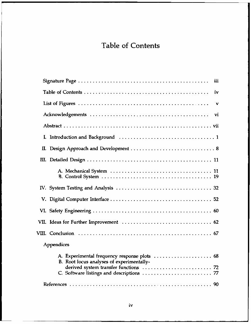
Table of Contents

Signature Page ............................................... iii

Table of Contents ............................................. iv

List of Figures ............................................. v

Acknowledgements .. ......................................... vi

Abstract .................................................... vii

I. Introduction and Background ................................. 1

II. Design Approach and Development ............................. 8

MI. Detailed Design ............................................ 11

A. Mechanical System ................................... 11B. Control System ....................................... 19

IV. System Testing and Analysis ................................. 32

V. Digital Computer Interface ................................... 52

VI. Safety Engineering .......................................... 60

VII. Ideas for Further Improvement ............................... 62

VIII. Conclusion . .............................................. 67

Appendices

A. Experimental frequency response plots .................... 68B. Root locus analyses of experimentally-

derived system transfer functions ........................ 72C. Software listings and descriptions ........................ 77

References .................................................. 90

iv

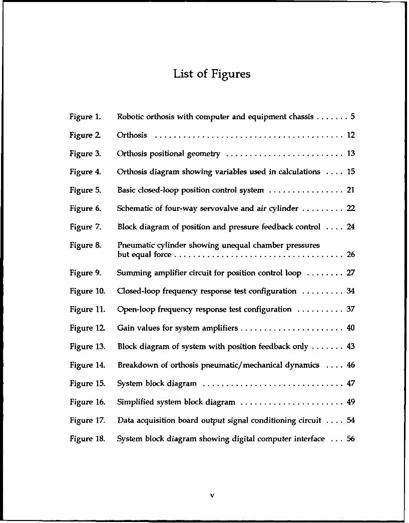
List of Figures

Figure 1. Robotic orthosis with computer and equipment chassis ....... 5

Figure 2 Orthosis . ........................................ 12

Figure 3. Orthosis positional geometry ......................... 13

Figure 4. Orthosis diagram showing variables used in calculations .... 15

Figure 5. Basic closed-loop position control system ................ 21

Figure 6. Schematic of four-way servovalve and air cylinder ......... 22

Figure 7. Block diagram of position and pressure feedback control .... 24

Figure 8. Pneumatic cylinder showing unequal chamber pressuresbut equal force .................................... 26

Figure 9. Summing amplifier circuit for position control loop ........ 27

Figure 10. Closed-loop frequency response test configuration ......... 34

Figure 11. Open-loop frequency response test configuration .......... 37

Figure 12. Gain values for system amplifiers ...................... 40

Figure 13. Block diagram of system with position feedback only ....... 43

Figure 14. Breakdown of orthosis pneumatic/mechanical dynamics .... 46

Figure 15. System block diagram .............................. 47

Figure 16. Simplified system block diagram ...................... 49

Figure 17. Data acquisition board output signal conditioning circuit .... 54

Figure 18. System block diagram showing digital computer interface ... 56

v

Acknowledgements

I am very grateful to Dr. Alan Schneider for providing me the opportunity

to develop this project from an idea to a working model, spending many hours

helping me to realize practical applications of control system theory. Many

thanks also to the UCSD Academic Senate for approving our proposal and

funding this research.

Eric Rollins, an engineering student, has been instrumental in the progress

of this research by designing and manufacturing the structure of the orthosis as

well as many other custom parts, and is responsible for converting each of the

figures in the body of this document from a crude sketch to a computer graphic.

I also wish to acknowledge Tom Phillips, AMES Electronics Technician, for

superior assistance in designing, building, and testing much of the circuitry

required to ope-'e, the robotic arm.

I would like to thank my wonderful parents for their loving support an'1

my father especially for spending countless hours with me editing and formatting

this document Thanks also go to Jim Braun for providing the computer and

software necessary to publish this document

Finally, special acknowledgement is deserved by the most important

person in my life, Brenda Jean Brogan, who not only provided extra motivation

and support throughout my Master's program, but who also gave me the most

beautiful daughter in the world last summer, Kristin Ann. I love you both very

much.

vi

ABSTRACT OF THE THESIS

Pneumatically-Powered OrthosiL and Electronic Control System

for Stroke Patient Rehabilitation

by

William K Brogan, Jr.

Master of Science in Engineering Sciences (Systems Science)

University of California, San Diego, 1993

Dr. Alan M. Schneider, Chair

This thesis presents the development of a system designed to manipulate

the upper extremity of stroke patients suffering from hemiplegia. The orthosis,

an aluminum structure built to be strapped onto a patient's paretic arm, is jointed

at the elbow to allow rotational motion of the arm. Compressed air provides the

force necessary to move the orthosis/arm combination through a selected motion

profile via a power cylinder activated by a pneumatic servovalve. Sensors located

on the orthosis and throughout the system provide feedback to circuitry which

precisely controls arm position.

vii

A digital computer with data acquisition capability provides software

control over several system parameters and generates a user-friendly interface to

the therapist performing the rehabilitation exercise. Measurements such as

velocity, acceleration, and differential pressure taken during various operating

modes can be used to calculate power, strength, range of motion, and degree of

muscle spasticity so that a time history of improvement for the patient may be

developed and used to study the effects of such therapy on stroke rehabilitation.

viii

I. INTRODUCTION AND BACKGROUND

Hundreds of thousands of Americans become victims of a disabling stroke

each year. Although many are too severely affected to benefit from standard

rehabilitation therapy, most patients will benefit from such therapy in varying

degrees. Stroke often leaves it's victim suffering from hemiplegia, paralysis of

one half of the body. Current rehabilitative techniques include passive motion of

the patient's unresponsive limb to improve range of motion and strength.

However, there seems to be a lack of scientifically-gathered quantitative

measurements dealing with stroke patient improvement over a course of time.

This is the underlying premise on which my research and the development of the

powered orthosis is based.

With our "robotic arm" orthosis, as I shall refer to it throughout this report,

we will perform extensive studies of stroke patient improvement over time based

on several measurable quantities recorded during therapy. Since this goal is a

long-term one, this thesis only covers the design approach and preliminary testing

of the mechanical and electronic systems of which the robotic arm is comprised.

A later section will describe recommended additions and improvements to the

system that will enable safe and practical use with actual stroke patients.

The original idea for this research came from Dr. Vernon L. Nickel [11,

retired Director of Rehabilitation at Sharp Rehabilitation Center, who suggested

that continuous passive motion of a stroke patient's disabled limb could possibly

increase the effectiveness of and shorten the ensuing recovery period. Research

i r =1

2

involving continuous passive motion (one of the functions this robotic orthosis

will provide) for the rehabilitation of a stroke victim's dysfunctional upper

extremity, together with quantitative measurements of progress, is almost non-

existent. The mechanism of continuous passive motion (CPM) in stroke patient

rehabilitation has not been fully exploited, although several studies have been

performed by associates of the University. However, these studies concentrated

on the lower extremities. In previous work, Dr. Schneider and others developed

a computer program that complemented a continuous passive motion device built

by a San Diego biomedical company for exercising and training the leg of a stroke

patient. [2] Favorable results from its use in a test with 31 patients are described

in a short paper by Blevins, Coutts, Lieber, Schneider, et. al. [3] Up to the present

time, over 100 patients have used this machine at Sharp Hospital, San Diego,

under the direction of Richard D. Coutts, M.D.

The "robotic arm" prototype as it currently exists is a machined aluminum

frame structure, hinged at the elbow, which can be strapped around a patient's

forearm and upper arm (see Figure 1). The forearm and upper arm sections move

relative to each other with the positioning force provided by a pneumatic (air)

cylinder. A similar-looking cylinder attached onto this power cylinder is a linear

potentiometer which provides a feedback voltage relative to the position of the

pneumatic cylinder rod. The compressed air required to power the cylinder is

provided by facility connections at a pressure of 80 pounds per square inch (psi).

This air is fed through a mist separator to remove excessive moisture, then

3

directly to the controlling component, called a pneumatic servovalve. The

servovalve is an electro-pneumatic device which uses a varying input voltage

produced by the electronic control system to output a proportional rate of air

flow to the air cylinder. This is the key ingredient in the ability of the system to

position the arm precisely to where it is commanded. The electronic control

system consists of the various devices and electrical signals required to generate

a desired motion profile for the arm, measure the arm's actual position, and use

any error between the two to cause the servovalve to correct the arm's position.

Specifically, this system includes a commercially available analog servo control

amplifier circuit designed to drive the servovalve, two pressure transducers

(sensors) which provide a differential cylinder pressure feedback signal to this

amplifier circuit, and position-sensing equipment used to generate the control

signal required. A rotary encoder (used to determine rotation angle) located at

the elbow joint and the linear potentiometer mentioned earlier provide different

forms of position feedback, either of which can be compared with the desired

position of the arm (based on a selected motion profile). A separate summing

amplifier circuit performs this comparison and outputs the resulting error signal

to the servo control amplifier circuit.

User-friendly, interactive software for an IBM-compatible personal

computer exists in preliminary form to create a desired motion profile for the arm

and will eventually be upgraded to perform the calculations necessary to

determine patient exercise parameters such as strength, energy, power, and range

4

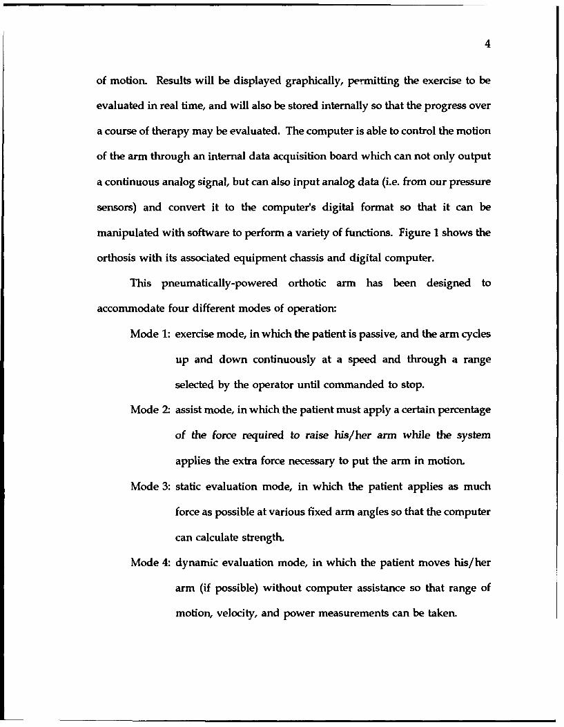
of motion. Results will be displayed graphically, permitting the exercise to be

evaluated in real time, and will also be stored internally so that the progress over

a course of therapy may be evaluated. The computer is able to control the motion

of the arm through an internal data acquisition board which can not only output

a continuous analog signal, but can also input analog data (i.e. from our pressure

sensors) and convert it to the computer's digital format so that it can be

manipulated with software to perform a variety of functions. Figure 1 shows the

orthosis with its associated equipment chassis and digital computer.

This pneumatically-powered orthotic arm has been designed to

accommodate four different modes of operation:

Mode 1: exercise mode, in which the patient is passive, and the arm cycles

up and down continuously at a speed and through a range

selected by the operator until commanded to stop.

Mode 2 assist mode, in which the patient must apply a certain percentage

of the force required to raise his/her arm while the system

applies the extra force necessary to put the arm in motion.

Mode 3: static evaluation mode, in which the patient applies as much

force as possible at various fixed arm angles so that the computer

can calculate strength.

Mode 4: dynamic evaluation mode, in which the patient moves his/her

arm (if possible) without computer assistance so that range of

motion, velocity, and power measurements can be taken.

5

Figure 1. Robotic orthosis with computer and equipment chassis

' m '

6

At the present time, the exercise mode (Mode 1) is fully functional. When

the computer program is started, the therapist is prompted to strap the orthosis

around the patients arm then move the arm/orthosis combination to maximum

flexion and extension angles to be achieved during the exercise. This angle data

is generated by the rotary encoder and inserted into the exercise motion profile.

Continuing prompts from the software ask the user for desired rate of motion,

any rest time at each extreme position, and the number of exercise cycles to

perform (one cycle defined as motion from the maximum extension angle to the

maximum flexion angle and back to maximum extension). The arm is

commanded to move at a constant speed to more closely resemble the motion

applied by a physical therapist.

Mode 2, assist mode, is still being implemented but is conceptually defined.

Since it can be calculated how much pressure in the cylinder is required to move

the orthosis and patient arm, the operator will select a percentage of machine

assistance from zero to one hundred which will preload the air cylinder with a

proportional amount of pressure. The patient then only needs to put enough

force into the orthosis to generate the remaining pressure in the cylinder which

will consequently cause the arm to move. This mode will allow the patient to

benefit from self-exercise at any level at which they are capable.

The static evaluation of Mode 3 has been partially demonstrated at this

point by sending the output of the two pressure transducers (which measure

pressure on both sides of the cylinder piston) to the computer and displaying a

7

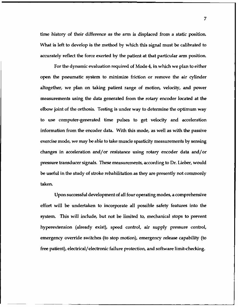
time history of their difference as the arm is displaced from a static position.

What is left to develop is the method by which this signal must be calibrated to

accurately reflect the force exerted by the patient at that particular arm position.

For the dynamic evaluation required of Mode 4, in which we plan to either

open the pneumatic system to minimize friction or remove the air cylinder

altogether, we plan on taking patient range of motion, velocity, and power

measurements using the data generated from the rotary encoder located at the

elbow joint of the orthosis. Testing is under way to determine the optimum way

to use computer-generated time pulses to get velocity and acceleration

information from the encoder data. With this mode, as well as with the passive

exercise mode, we may be able to take muscle spasticity measurements by sensing

changes in acceleration and/or resistance using rotary encoder data and/or

pressure transducer signals. These measurements, according to Dr. Lieber, would

be useful in the study of stroke rehabilitation as they are presently not commonly

taken.

Upon successful development of all four operating modes, a comprehensive

effort will be undertaken to incorporate all possible safety features into the

system. This will include, but not be limited to, mechanical stops to prevent

hyperextension (already exist), speed control, air supply pressure control,

emergency override switches (to stop motion), emergency release capability (to

free patient), electrical/electronic failure protection, and software limit-checking.

II. DESIGN APPROACH AND DEVELOPMENT

Several options for powering the orthosis were considered during the

conceptual design stage of this project Electric motors were first discussed to

directly drive the angular motion of the orthosis about the elbow joint, but a

desire to minimize weight and protuberances prevented us from finding a

suitable device. It was also recognized that a complex gearbox and/or clutch

arrangement would be required in order to operate the orthosis in all of the

planned modes, specifically the dynamic evaluation mode where all possible

friction sources should be removed. Among the advantages of using a motor

drive however are readily-available velocity feedback (with an attached

tachometer), fewer system components, and a simpler system to analyze.

Although the possibility of incorporating electric motors still remains a viable

option, we decided to investigate other practical automation techniques.

The use of hydraulics was then considered because of its very high force

output capability and ability for precise positioning control. However, it was

determined that the very high pressures commonly found in hydraulic systems

would prove to be a potential safety problem when used in such close proximity

to human beings. Since a viscous fluid is used to transmit power in the system,

we also felt that oil leaks would be inevitable, dangerous, and messy. Pricing

components for a hydraulically controlled system revealed high costs which

would have quickly depleted our budget.

8

9

We learned that several companies manufacture pneumatic servovalves,

devices capable of using compressed air to produce the precise positioning

required of our feedback control system. With a suitable electronic controller, a

pneumatic servovalve can control a load with the accuracy normally only found

in comparable hydraulic servo systems. Pneumatic systems however are limited

to smaller loads since the standard maximum air pressure available is normally

only 120 psi. We knew that the compressibility of air could present some

problems, but decided to test a pneumatic servovalve and associated servo control

amplifier anyway. Since compressed air was available via facility connections both

in our engineering laboratory and in the Veterans Administration Medical Center

physical therapy room, it was felt cost saving could be realized by requiring less

machinery. For instance, a costly, loud, bulky air compressor is no longer

required whereas it would have been if facility air was not available or if we had

decided to use hydraulics. Consideration must be given to future locations where

this system may be used, which may not have compressed air available through

facility connections, such as in some rehabilitation clinics or smaller hospitals.

This is one reason why the incorporation of electric motors may still be the best

overall method of providing power to move the orthosis if the proper

transmission system can be devised.

During the Spring quarter of 1992, a team consisting of four undergraduate

engineering students (Eric Rollins, Steve Haase, Michelle Conlay, and Rick Batt)

took initial requirements for design of the robotic arm from Dr. Schneider and

myself and produced, over the course of an eight week class, the aluminum

10

orthosis structure and the circuitry for reading the elbow joint's optical encoder

data. Complex initial specifications including wrist rotation and a master/slave

concept using the patients good arm to control the orthosis on the dysfunctional

arm yielded to a more practical design involving just one degree of rotational

freedom at the elbow joint. It was felt that once the mechanics and the control

system were fully understood and developed for this approach, it would be more

efficient to then incorporate more complex modifications.

My work with this robotic orthosis project has concentrated on using the

student team's mechanical orthosis to design, develop, and integrate a suitable

pneumatic control system so that the arm could eventually be used in the four

desired modes previously mentioned.

III. DETAILED DESIGN

The robotic orthosis can be broken down into two major design categories:

the mechanical system and the control system. Discussion of the digital interface

will be deferred until Section V.

A. MECHANICAL SYSTEM

The primary mechanics of the orthosis at present include the hinged,

aluminum structure itself as well as the linkage between the forearm and bicep

sections provided by the pneumatic cylinder body and its piston rod (Figure 2).

The device is allowed to rotate about the elbow joint with very low friction

through use of high-precision ball bearings. The cylinder mounting locations on

both sections of the orthosis are pin connections so that as the arm sweeps

through its range of motion the pneumatic cylinder can freely adjust its relative

position while its length varies. A 100-degree angular range of motion from full

extension to full flexion was originally sought, but the geometry of the mounting

locations and the cylinder size has limited us to about 93 degrees of arc. The

cylinder body mounting collar may be used to adjust the maximum extension

angle (and correspondingly the maximum flexion angle) while retaining the 93

degree range of motion. All analysis and initial testing were performed with the

cylinder positioned so that the maximum extension occurred at zero degrees

(when the forearm section and the bicep section are at an angle 180 degrees

relative to each other). Refer to Figure 3 for a graphic description of the rotation

11

12

Figure 2. Crthosis

13

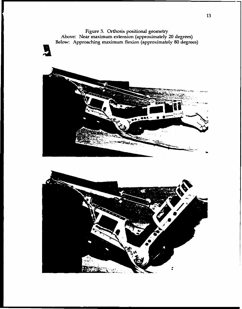
Figure 3. Orthosis positional geometryAbove: Near maximum extension (approximately 20 degrees)

Below: Approaching maximum flexion (approximately 80 degrees)

14

angle, 0, showing the orthosis near maximum extension and then approaching the

93-degree maximum flexion angle.

To find the smallest cylinder possible that would give us this range of

motion, the distances between the adjustable cylinder mounting bracket locations

had to be measured when the arm was at both maximum extension and at

maximum flexion. We found that with the mounting brackets in their closest

position toward the elbow joint we could achieve an acceptable range of motion

with a cylinder having eight inches of stroke. The reason the smallest possible

cylinder is necessary is not only for aesthetic quality but because if it were too

long the rear part may contact the patient's shoulder.

The next consideration for sizing the cylinder was determining how much

force it would be required to transmit given a constant supply pressure. The

variable here is cylinder bore, or diameter, which directly relates to piston area

and therefore force output (force equals pressure times piston area). The

following analysis determines FL, the load force which must be applied by the

piston to hold the arm in static equilibrium against gravity. Since the arm will

be commanded to operate through a motion profile which requires a constant

velocity and no acceleration, inertial forces can be ignored. Once the maximum

force is calculated, the proper cylinder can then be selected

Referring to the free-body diagram of Figure 4, in e, !,brirnum the sum of

the moments about the elbow joint is zero:

SFL sin azo,, = mg cosO

from which we find:

15

Figure 4. Orthosis diagram showing variables used in calculations

cylinder

Sdistance fromelbwji pointnpivot • r a

point u fo rr cn.e WRIST

~ -- /, ditac fro elo Jon to bie pio

SHOULDER bicep section ELBOW forearp section Mg coseJOINT W-mg•

FL ,. -ood force component normal to IFL. - load force component parallel to JFl. - cylinder load forceI-= distance from elbow joint to forearm pivotJl - distance from elbow joint to forearm center of gravityu - distance from elbow joint to bleep pivotr -, distance from bicep pivot to forearm pivot

r., - corrected distance from cylinder mounting bracket to forearm pivotk - height of cylinder centerline above bicep pivote - rotation angle of forearm relative to horizontalm = combined mass of orthosis forearm section and patient forearm

16

F- • 1mgcosOFL- 9,sgric O

9sina corr

It can be seen that the maximum load force will occur when 0 = 0" (when

the arm is at full extension) because here a (and thus sin a) will be its smallest

value and cos 0 will be at its greatest. The variables 0, m, and •1 are all

measurable which leaves the problem of determing a.

From the law of sines,

r U

siny sina

so

a=arcsin( usiny)r

and

acmn=arcsin ( usiny,,)

We can find y. from the law of cosines (r. is measurable)

y x=arccos( 2u_

Using values measured from the orthosis and taken from CAD drawings

r. = 15.94 inches

9 = 7.026 inches

u = 9.747 inches

we calculate that a.. = 21.47 degrees.

17

Correcting for the fact that the bicep section's cylinder mounting collar raises the

centerline of the cylinder a height k above the pivot point (Figure 4),

rcorr= (Ir2,.-k2) 1A

and

acorr== +arcsin( krcorr

With k measured as 1.05 inches, we get a.,, = 25.26 degrees.

The orthosis forearm section weighs approximately 0.75 lb, and a volume

displacement test performed on my forearm showed its weight to be about 3.0 lbs

(or about 1.9% of my body weight, assuming arm density of 1.053 g/cm3).

Adding a few pounds to these values to account for the maximum expected

forearm weight for a large person and to provide for growth to the orthosis, I

chose 6.0 lbs as the maximum weight the cylinder would have to lift. This weight

acts at a distance 1, (center of gravity location) from the elbow joint which was

determined for the orthosis forearm section by a basic "knife edge" balance test

with the adjustable forearm extender in the furthest position. It was then

assumed that for our maximum expected patient forearm size the center of

gravity location would be no further than 10 inches from the elbow joint, giving

us the worst case distance for the orthosis/patient arm center of gravity location.

With that,

18

FL_ (10inches) (61bs)cosO =20lbs(7. 026inches) (sin25.260)

To ensure enough force would be available to provide a stiff, responsive system

even at worst-case conditions and to overcome frictional forces, we decided that

the pneumatic cylinder should have a force output capability of about 40 pounds

at a supply pressure of 80 p.s.i. (pounds per square inch). Most cylinders are

rated for slightly different force outputs on the extension and retraction strokes

due to the small area lost to the piston rod. Since we would require the highest

force moving the orthosis from maximum extension to maximum flexion (because

of gravity) which is the direction powered by this smaller area of the piston in

our particular configuration, we chose a cylinder which provides about 40 pounds

in that direction (and obviously provides slightly more in the opposite direction

due to the full area available on the piston). The cylinder we are using has a bore

size of 0.75 inch. At this point in the development of the mechanical system the

possible effects of muscle spasticity on the required force output of the cylinder

were not taken into consideration. A cylinder with a larger bore could easily be

substituted to provide more force if necessary.

Early in the design of the robotic arm we assumed incorrectly that the

patient's arm should be exercised using a sinusoidal velocity profile, providing

a slightly higher speed in the middle of the range of motion than at both

extremes. For this reason analyses were accomplished to find the velocity and

19

acceleration of the orthosis through its arc for use in load force calculations and

determination of mechanical time constants. Per Dr. Lieber's suggestion, the

orthosis is now commanded to move only at constant velocities, which eliminates

the need to present those analyses in this report. They are on file with Dr.

Schneider for reference.

B. CONTROL SYSTEM

Because there exists the requirement to maintain the orthosis precisely

along a path or at a position commanded by the user-defined motion profile, a

closed-loop feedback control system was necessary to measure actual arm position

and compare that with the commanded arm position then perform any

corrections resulting from their difference.

Since the power transmission medium is a fluid in our case, the control of

the system is more complicated due to the compressibility of the air. Only in the

past ten years or so has the technology become available to provide precise

positioning control of pneumatic systems. The availability of high-speed

controlling electronics and pneumatic servovalves allows the closed-loop control

of a system by quickly and continuously restoring equilibrium across the piston

in the power cylinder should it change from its commanded value [4]. The term

servovalve merely refers to the fact that the valve's output or response is directly

proportional to its input signal from feedback sensors which may be constantly

varying in order to bring the system to its commanded position, velocity, etc. [5]

20

In fact, closed-loop control provides automatic compensation for changes in

command signals, friction, temperature, transient loading, and leakage.

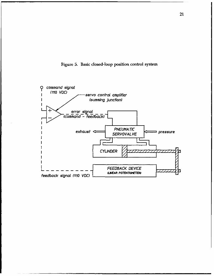
A basic closed-loop position control system is shown in Figure 5. Our

robotic orthosis uses this configuration as well as several other devices for sensing

and control which will be discussed later. From the figure we see that the servo

control amplifier produces an error signal which is the difference between the

command signal (a voltage representing the desired position) and the feedback

signal (also proportional to position). This error signal will cause the servovalve

to displace its inner spool (see Figure 6) enough to bring the pressure in the

cylinder to a point where the piston moves and the feedback device reads exactly

the same voltage as the command signal. When this occurs, the error signal

becomes zero and the orthosis, attached to the piston, is now static until the

command signal changes.

The servo control amplifier is a commercial circuit board which not only

accepts the command signal and feedback inputs and produces the servovalve

driving signal, but also contains potentiometers for adjustment of the gains for the

feedback and error signals (among others). This provides the proportional control

which improves system performance.

Using a 5 kfQ linear potentiometer (which is mounted above the pneumatic

cylinder) to generate a voltage proportional to the piston rod position and

inputting this signal to the servo control amplifier, we found that the motion of

the orthosis under a sinusoidal command signal was slightly jerky. Mr. Richard

21

Figure 5. Basic closed-loop position control system

command signal±0 Vservo control amplifier

(summing junction)

error signal

- (command - feedback)

exhaust SEVOALVE pressure

t 'CL FEEDBACK DEVICE

feedback signal (±10 VDC)

22

Figure 6. Schematic of four-way servovalve and air cylinder

Sdouble-acting air cylinder (actuator)

valve actuation coi four-way servovolve

supply pressure

23

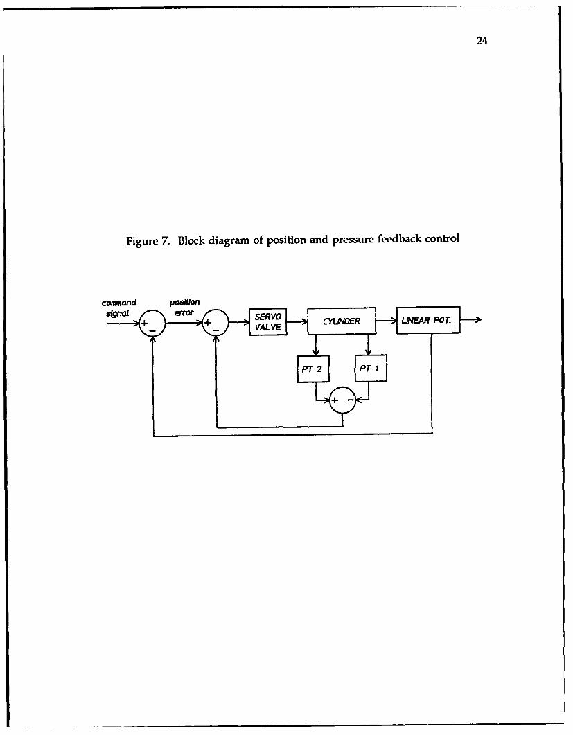
Duder of Dynamic Valves, Inc. [6], the company from which the servovalve and

servo control amplifier were purchased, suggested that improvements in control

loop stability could be achieved by using a dual closed-loop configuration with

pressure feedback as the inner loop and position feedback as the outer loop, as

in Figure 7. This is true because with position feedback only, the error signal

causes the servovalve to output a linear flow rate which in turn moves the

orthosis at a proportional velocity. However, if the position error is used as the

input signal to a pressure feedback loop, the output of the servovalve will

generate a force proportional to the signal that will drive the position error to

zero. Laboratory tests under both conditions confirmed that using both pressure

and position feedback provided a smoother, more stable orthosis movement

Pressure feedback was introduced by using two pressure transducers which

were connected in-line with the air hoses coming from both outputs of the

servovalve and going to both chambers of the pneumatic cylinder. These

transducers are designed to output 0 to 5 VDC when subjected to pressures of

between 0 and 120 psi. Since we are only using a maximum pressure of about

85 psi, the maximum output signal from the units is only about 3 VDC. For this

reason the FEEDBACK GAIN potentiometer on the servo control amplifier board

was adjusted to amplify this signal so that it ranges between 0 and 10 VDC,

matching the command input signal. The transducers were wired so that one

produced a positive output voltage while the other produced an equivalent

negative output voltage when connected to the compressed air supply. This was

24

Figure 7. Block diagram of position and pressure feedback control

cowand positon

VLEO

25

necessary because each output was connected to one of two feedback input

terminals on the servo control amplifier, the sum of which was produced and

used as the inner control loop feedback signal. In effect, we were using the

circuitry available on the servo control amplifier board to create a differential

pressure measurement since we did not have available such a transducer. The

important concept is that the difference in pressure between both chambers in the

pneumatic cylinder is a measurement of the force balance on the piston, and

depending on the size of the load the piston is required to move, whether the

piston is in motion (note that an equal force balance across the piston will require

slightly different pressures in both cylinder chambers due to the smaller piston

area where the piston rod is connected-see Figure 8).

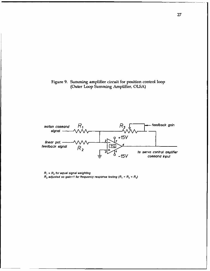
Because the addition of pressure feedback as the inner control loop

required the two available feedback inputs on the servo control amplifier boaraj,

a separate summing amplifier was necessary to add the motion profile command

signal with the linear potentiometer position feedback signal. This outer control

loop creates the position error signal used as input to the inner pressure control

loop. The summing amplifier circuit, shown in Figure 9, uses a standard

integrated circuit operational amplifier.

Although another sensor, the optical rotary encoder mounted on the

orthosis elbow, was available for use in the control system it was not incorporated

into the analog servo amplifier circuit because of its inherent digital output Its

use will be described in Section V, Digital Computer Interface.

26

Figure 8. Pneumatic cylinder showing unequal chamber pressures but equalforce

p Ap piston p-

piston rod chamber 1 chamber 2(requires slightly higher pressure)

0SQchamber I piston chamber 2 pistoneffective area effective area

27

Figure 9. Summing amplifier circuit for position control loop(Outer Loop Summing Amplifier, OLSA)

motion command P1 R3 _ + feedback gain

linear pot.7feedback signal 62

d k nto servo control amplifier

._15V command input

R, = R2 for equal signal weightingR, adjusted so gain=1 for frequency response testing (R, = R2 = RJ)

28

In order to tune the control system so that the orthosis would respond to

different inputs (i.e., impulse, step) in an acceptable manner, the amplifier gain

values had to be properly adjusted. The outer loop summing amplifier gain was

set to 1 so that system stability could be solely adjusted by the ERROR GAIN

potentiometer found on the servo control amplifier circuit board. [NOTE: A

procedure for matching magnitudes of the feedback signals and command signals

on the servo control amplifier board must first be performed per the operations

manual [7]. This is done to ensure the maximum feedback signal with gain (from

the pressure transducers) is equal in magnitude but opposite in polarity to the

maximum command signal (from the outer loop summing amplifier)]. With no

command signal input provided to the outer loop summing amplifier, the system

moves the orthosis to a position which generates zero volts from the linear

potentiometer. Since the linear potentiometer is powered with +10 VDC at one

end and -10 VDC at the other, its center position will produce an output of zero

volts (an orthosis angle of about 45 degrees).

Movement of the arm by brute force while it is being held static generates

a voltage from the linear potentiometer proportional to the displacement. Since

there is no command signal present (0 volts), the output of the outer loop

summing amplifier is equal to but opposite in polarity from this linear

displacement signal and is sent to the inner pressure control loop. The servovalve

immediately responds by increasing the pre-sure in the respective cylinder

chamber to force the piston back to the center position. An impulse response was

29

simulated by forcing the arm away from its neutral central position and releasing.

An oscillatory time response was observed initially. Adjusting the ERROR GAIN

potentiometer on the servo board, the time response to this impulse input was

optimized so that oscillations were eliminated but not at the expense of

introducing too much damping (thus creating too slow of a response). To verify

acceptable response to a step input, a constant voltage was applied to the outer

loop summing amplifier command input The system responded quickly and

properly by positioning the orthosis at an angle which produced an equal but

opposite voltage from the linear potentiometer with no visible oscillations.

With the control system configured as described above, the proposed

exercise mode of the robotic orthosis is now basically functional. This mode

merely requires a user-defined motion profile to be input as the command signal

to the outer loop summing amplifier. The arm will move accordingly and can

thus be used as a continuous passive motion device. A ±10 VDC sinusoidal input

was initially used to move the arm in this mode, but later a computer program

was developed that can command the arm to move through any programmed

motion profile.

This control system configuration also directly supports operation of the

static evaluation mode in which the arm is held at a specified position and the

patient uses his/her strength to try to move the arm. With a constant voltage

command signal applied at the outer loop summing amplifier, the linear pot will

hold the arm in a specified position within its range of motion. Any attempt to

30

displace the arm from this position will create an error signal from the position

control loop and cause the servovalve to increase pressure in the appropriate

cylinder chamber to maintain the commanded position. This pressure change can

be measured at Test Point B on the servo control amplifier circuit board [7]. This

signal, therefore, has a direct correlation to the force input to displace the arm,

and thus is a measure of the patient's strength. This relationship has not yet been

quantitatively defined. Calibration using a load cell has been suggested as one

method of determining this force to verify it has a linear relationship with the

pressure change across the cylinder piston.

It has also been suggested that measurement of a stroke patient's bicep

muscle spasticity would be useful. Laboratory experiments show that while the

arm is in the passive exercise mode described earlier that any resistance

encountered along the arm's trajectory will create a corresponding pressure

increase in order to overcome and maintain the commanded position. This in

turn creates a voltage signal that can be used in the measurement of the

magnitude of spasticity. Difficulties that may be encountered with this

measurement, however, include any volitional, or desired, muscle activity by the

patient which may taint the spasticity measurement

Some prelimninary analysis has been performed by Dr. Schneider to

determine the proper control system configuration necessary for the "percent

assist" mode of orthosis operation. Here the pneumatic cylinder is preloaded

31

with a selected fraction of the force required to place the arm in motion and

therefore may require pressure feedback only in order to operate properly.

IV. SYSTEM TESTING AND ANALYSIS

With the control system configured as described in the previous section

such that the arm follows a commanded motion profile (passive exercise mode),

the system transfer function was characterized by performing various frequency

response tests using a sinusoidal signal with known magnitude and frequency

applied to the outer loop summing amplifier. The voltage signal from the linear

potentiometer was measured as the arm oscillated through its range of motion,

then the frequency of the sine wave was increased. This process continued until

the arm was oscillating so fast and its amplitude was attenuated by so much that

it appeared to be at rest. These data were used to create a frequency response,

or Bode, plot of the system. From this plot, approximations to the actual system

transfer functions can be made. Once transfer functions are available, standard

control system analysis techniques can be used to design any required

compensation into the system to make it perform in a specified manner. The

following test data and analyses are relevant only at a supply air pressure of 80

psi and with the amplifier gains set at the values discussed later in this section.

A Hewlett-Packard Model 3312A Function Generator was used to provide

the sinusoidal command input. The sine wave output amplitude was adjusted

initially using a digital multimeter to span a range of +10 VDC to -10 VDC,

thus matching the linear potentiometer's output range. Once this signal was

input to the outer loop summing amplifier however, it was causing the orthosis

to strike its mechanical stops (cylinder piston extreme points). This was due to

32

33

the fact that the linear potentiometer output was actually somewhat less than ±10

VDC due to inaccuracies of the voltage-dropping resistors placed in-line with it

(to drop the ±15 VDC power supply voltage from the servo control amplifier

circuit down to the desired ±10 VDC). This problem was overcome by simply

reducing the sine wave magnitude from the signal generator until a shorter range

of motion was achieved. The outpit of the function generator was input to a

Hewlett-Packard Model 54500A 100 MHz Digital Oscilloscope so that its

amplitude and frequency could be easily determined after any adjustments.

CLOSED-LOOP TEST

The output of interest for the closed-loop system test is from the linear

potentiometer (See Figure 10). This signal must still be connected to the outer

loop summing amplifier to ensure closed-loop operation, so a probe was used to

pick off this signal and send it to the other available oscilloscope input channel.

Once the function generator was started, both signals were available on the scope.

The test was initiated using a very low frequency (0.01 Hz) then a manual sweep

of increasing frequencies was performed. At each selected input frequency, the

magnitude of the output oscillation was measured from the linear potentiometer

signal. As the frequency increased past 1.3 Hz, it was evident that the output

was being attenuated relative to the input Finally, at 9.0 Hz, the output was so

attenuated that the magnitude was indiscernible on the oscilloscope. Graphical

display of these data is available in the form of a Bode plot that can be found in

34

Figure 10. Closed-loop frequency response test configuration

OLSA

linear pot. feedbackOLSA - outer loop summing ampliferPT - presaure transducer

35

Appendix A-1. The vertical axis of the plot depicts the magnitude of the ratio of

the output voltage to the input voltage in decibels (dB), or

201oglo ( output voltage)input voltage

From the plot we see (using the asymptotic approximations for the actual

test data) that our closed-loop control system behaves as a third-order system

because of the first-order (-20 dB/decade) attenuation slope at frequencies higher

than about 1.3 Hz (8.17 radians/sec) and the second-order (-40 dB/decade)

attenuation after about 3.0 Hz (18.85 rad/sec). The closed-loop transfer function

(CLTF) could then be approximated as (assuming a damping factor of 0.5)

CLTF= 1S +1)[( S )2+ s +1]

8.17 18.85 18.85

or simplified as

CLTF= 2902.85(s+8.17) (S 2 +18.85s+355.32)

Since the arm will be operated at frequencies in the range of approximately

0.05 Hz to 0.3 Hz, our analysis shows that the bandwidth of the system is more

than adequate (the output of the system will exactly match the input) and

therefore no compensation is required. This experimentally derived closed-loop

36

transfer function will be compared to an analytically derived model (using open-

loop test data) at the conclusion of this section.

OPEN LOOP TESTS

More useful information can often be gained from open-loop frequency

response testing than from closed-loop tests. An open-loop test can help us

determine the actual transfer functions of any number of individual components

or groups of components within the system. Once characteristics of the open-loop

system are known (i.e., the location of poles and zeroes), the methods of classical

control theory can be applied to dictate the desired system characteristics once the

loop is closed. A closed-loop frequency response on the other hand merely

displays how a complex system is responding with feedback under a given, static

set of conditions.

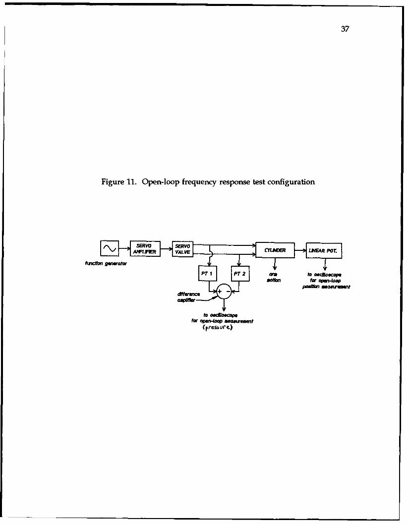
Two separate open-loop frequency tests were performed; one in which the

output of the pressure transducers was measured and the other in which the

output of the linear potentiometer was measured. For both tests, the feedback

loops from the pressure transducers and the linear potentiometer were opened

(See Figure 11). The lack of position control made the performance of the

frequency response tests very difficult as the center point for the arm's range of

motion tended to drift. Since unmeaningful data would result if the arm reached

the mechanical stop at either extreme position, I had to constantly adjust the

amplitude of the input sine wave (using the vernier control on the function

37

Figure 11. Open-loop frequency response test configuration

Mf U9E VAV OR• POT.

to oedbeacpefor qmn-IW meai"nmnt

(pressure.)

38

generator) to try to keep the arm oscillating in an acceptable arc long enough to

read a valid output magnitude signal.

In order to use the output from both pressure transducers now that they

are disconnected from the servo control amplifier circuit board's feedback inputs,

a summing amplifier was required to add the two signals to again create a single

differential pressure signal (remember, the pressure transducers are wired so that

they produce signals opposite in polarity to each other). The outer loop summing

amplifier was used since it was not required for these open loop tests.

A procedure similar to that for the closed-loop test was used for

performing the frequency response test of the open-loop system. The function

generator was started and the appropriate output response signal from the control

system (position or pressure) was measured and compared to the input signal

magnitude. The frequency was increased from as low as practical to as high as

output magnitude measurements were still discernible. See Appendix A-2 and

A-3 for the Bode plots of these open-loop tests. It should be noted that these

experimental measurements are by no means absolute; each time the test was

performed slightly different values resulted. These Bode plots reflect the

experience of several test runs each and are what I consider to be the most

accurate data. During these tests, I also monitored the input-output phase

relationship on the oscilloscope at each measurement. The resulting waveform

(when the scope is placed in the "X-Y" display mode) is known as a Lissajous

pattern and gives a qualitative measure of the phase lag of the output versus the

39

input signal. According to Ogata [81, experimental phase measurements are not

as reliable as magnitude measurements due to their sensitivity to slight changes

in system parameters and to system non-linearities. However, they can be used

to gain some insight into the complexity of the system. Rough sketches of the

Lissajous patterns as seen on the oscilloscope screen are available with the raw

test data on file with Dr. Schneider.

In order to perform a meaningful analysis from these Bode plots, any

amplifiers in series with the components whose transfer functions are sought

must have their gain values known. These gains can then be removed from the

measured open-loop transfer function to reveal the component's true gain value.

This gain measurement test was performed using a Hewlett-Packard Model 6235A

Triple Output Power Supply that supplied a constant voltage which I chose

arbitrarily to be +3.0 VDC. This voltage was applied to the various amplifiers in

our system, including the custom open loop summing amplifier and the various

amplifiers on the servo control amplifier circuit board. Figure 12 shows these

gain values as they appear in the system block diagram. It is important to note

that the experimental frequency response measurements are based on these values

of amplifier gain that were chosen to optimize system response to inputs as

mentioned earlier. Any change to these values by adjusting the appropriate

potentiometers will alter the frequency response test output.

It is now possible to use the Bode plots to again perform system

characterization, the determination of a system's transfer function from

40

Figure 12. Gain values for system amplifiers

servo control amplifler drcult board

outer loop summing anla test pt. A test pt. C

#1. -fx CYLINDIER. APNO

K•,, -1 Kj-=-4.35 K,- -155 ORTHO-S I$

E #2K,- -0.745

pressure transducer (PT) feedback:

linear potentiometer feedback

a gain values are negative because of Inverting amplifiers

"KoLsA, K, K2. K3 . K4 in vols/volt

41

experimental response data. First we will use the output of the open-loop

position measurement test found in Appendi>, A-2. It should be mentioned that

the asymptotes drawn on the Bode plot (which must be multiples of ±20 decibels

per decade) are only visual approximations to actual test data. The asymptotic

approximations I used show an initial first-order slope (an integrating effect of the

servovalve with a constant voltage input signal creating a continuous, cumulative

flow of air) with two other first-order breaks occurring at about 3.5 Hz (22

radians/sec) and 6 Hz (37.7 rad/sec). This reveals to us that the open-loop path

for position control is third-order, as suggested by deSilva [51 and McCloy [91 for

a pneumatic system similar to ours. The gain of the system is found by noting

where the plot intersects a frequency of I rad/sec (0.16 Hz). In this case it is at

31.5 dB, or converting to natural numbers as a gain factor K,

201og1 0 K=31.5dB

31.5

K=10 20 =37.58

Using the values in radians/sec for further calculations, the open-loop system

transfer function (without pressure feedback) can be written as

Y(s) 37.58OLTFPitio- X(s)" (- 1) S +1)22 37.7

42

which when normalized yields

_YLT _( 31158.68OLTPPiti "-O X(s) s(s+22) (s+37. 7)

where Y(s) represents the Laplace transform of the output position from the linear

potentiometer in volts and X(s) the commanded input position in volts. This

transfer function is a conglomeration of all system gains and dynamic

characteristics in the open-loop forward path. A quick method for checking

stability of this system when the position feedback loop is close .. -iming no

pressure loop) is to perform a root locus analysis of the above transfer function.

This is done in Appendix B-1 which shows that the closed-loop system with

position feedback only is stable (the closed-loop poles are to the left of the vertical

axis), although very little margin remains. In fact, the system can remain stable

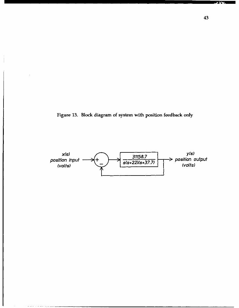
only if gain is increased by a factor less than 1.59. Figure 13 shows the block

diagram for this system.

From the open-loop pressure measurement test Bode plot (Appendix A-3)

we perform a similar analysis. Theory did not predict the very high gains

measured at frequencies below 1 H7, but this was most likely due to the very

slow rate at which the servovalve was commanded to cycle back and forth thus

allowing full air flow to the cylinder, in turn forcing the piston to its extreme

position. Thus, if we neglect this portion of the Bode plot as not being inherent

to the system dynamics, we simply find a fiat response (constant gain of about -

3 dB) with a first-order break at about 6 Hz (37.7 rad/sec), a very convenient

43

Figure 13. Block diagram of system with position feedback only

x(s) _31158.7 ys)position input position output

volts) (volts)

44

location keeping in mind this was also the location of a break frequency from the

open-loop position measurement Bode plot. This constant gain of -3 dB converted

to natural numbers gives

201og1 oK=-3dB

-3

K=10 20 =0.708

and a transfer function can now be written for this open-loop path as

OLTFPressure= P (s) 0.708

X(s) 3- ) +1~37.7

which when normalized yields

0LTF _P(s)_ 26.69

O pressure X(s) s+37.7

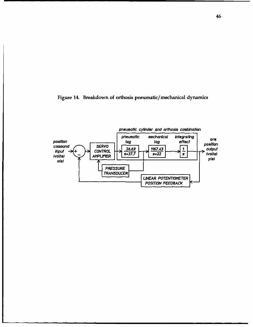
Knowing this transfer function helps us deduce the transfer functions and

system dynamics of the individual components of the pneumatic/mechanical

system. For example, we can see now from Figure 14 that the response of the

orthosis is dependent on three distinct system characteristics; pneumatic lag,

mechanical lag, and an integrating, or cumulative, effect.

Because the open-loop position and pressure tests both generated a first-

order exponential decay term of

45

G,(S) -s+37.7

we can consider this term the pneumatic time constant term

?pneumatic- 1=0. 027 secondsPnema~c37 .7

or the inherent delay in response due to the transmission of power via

compressed air. The remaining first-order term would then be the mechanical

lag, or delay, due to the inertial forces, friction, and other non-linearities integral

to the mechanical arm

=-n21 =0.04 5secondsmechanica-l22

and is almost double the delay of the pneumatics. Because we know the gain of

the open-loop position transfer function to be 31,158.68, we can divide this value

by the gain of the first first-order term found as the open-loop pressure transfer

function (26.69) to find a gain value for the second first-order term within the

system of 1,167.43 (shown in Figure 14).

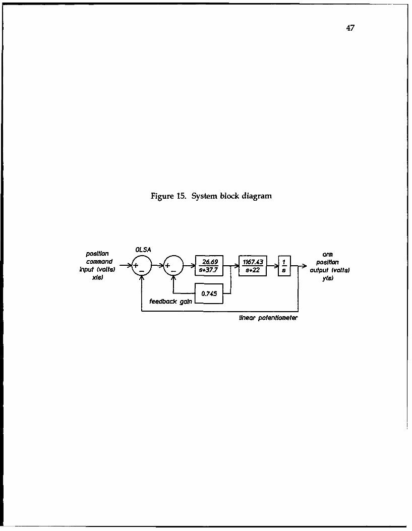
Now that the individual contributions for each component of the system

are known, we can close both the pressure feedback loop and the position

feedback loop and analytically determine the effects of pressure feedback on the

system response characteristics. The system block diagram is shown in Figure 15.

46

Figure 14. Breakdown of orthosis pneumatic/mechanical dynamics

pneumatic cylinder and orthosis combination

pneumatic mechanical integrating armposition lag lag effect positioncommand " RVut "+ CONTROL 26.69 1167.43 1 output(volts)• A+PLIOER s-37.7 s+22 s (volts)

(Vols) APURR LL-------- iy(G)

| TRANDUCERI LINEAR POTENTI0O4ETF_.R

POSITION FEEDBACK

47

Figure 15. System block diagram

position OLSAcommand + + 26.69 1167.43 1 position

Input (volts) - 377 s+22 a output (volts)xrs) y(s)

feedback gptneImI

linear potentiometer

48

The inner feedback loop can be simplified by finding its closed-loop transfer

function from

CLTF=_ G(s)

I +G(s) H(s)

as

26.69CLTFinnerloop= _ s+37.7i + (26.69) (0.745)

s+37.7

or simplified as

CLTFi op 26.69CLTF10v S+57.58

which when combined with the other components in the forward path yields the

open-loop transfer function

G(s) 31158.68s(s+22) (s+57.58)

and the simplified block diagram shown in Figure 16.

Referring to the block diagram of Figure 13, which does not take into

account pressure feedback, we can see the similarity with this system containing

both pressure and position feedback. A root locus analysis of the system transfer

function which does include pressure feedback is given in Appendix B-2 This

analysis reveals that the addition of pressure feedback to the system as the inner

control loop has benefitted the system by increasing its relative stability (the

system can now tolerate a gain multiplier of 3.24 versus only 1.59 without

49

Figure 16. Simplified system block diagram

OLSAposition armcommand +__31158.7__ position

input (volts) s-s+22)(s+57.58) output (volts)x(s) y(s)

linear potentiometer

50

pressure feedback). System damping was also affected positively by a slight

increase in its value which helps control oscillations.

An interesting check can now be performed by comparing this semi-

analytically derived closed-loop system transfer function (found from Figure 16

using unity feedback, or H(s) = 1)

CLTF= G(s) _ 31158.681+G(s)H(s) (s+67.66) (s 2 +l11.92s+460.2)

to the experimentally determined closed-loop system transfer function derived

from the Bode plot in Appendix A-I,

CLTF= 2902.85(s+8.17) (s 2 +18.85s+355.32)

Although there is an obvious discrepancy among the gains (a factor of 10.73) and

the loýcation of the real poles, the complex conjugate poles of both transfer

functions are quite similar. Such errors may be due to test inconsistency,

improper gain measurements, system non-linearities, and various other factors.

The usefulness of this comparison as well may be limited.

With the system transfer function now available, it is possible to alter

system response characteristics if desirable through implementation of

proportional, integral, and/or derivative (PID) control algorithms. At the present

this is not required because of acceptable system response but may be desirable

to implement in the future.

51

Before this section is concluded, it should be mentioned that the dynamic

characteristics of the servovalve and the pressure transducers were neglected in

this section's frequency response analyses because of their high bandwidth. The

servovalve has a rated bandwidth (frequency up to which the components output

replicates its input, or a flat frequency response) of 90 Hz and the pressure

transducers are rated to about 100 Hz, both much higher than our system was

required to respond (pressure transducer data was obtained from the

manufacturer, Wiancko Engineering Co. of Tarzana, CA).

V. DIGITAL COMPUTER INTERFACE

Once it was determined that the robotic orthosis system was properly

responding to commanded inputs, transition over to digital control was desired.

Using a computer as an interface between the operator and the controlling

electronics is an advantage not only in that it makes the system more user-

friendly through use of custom software, but also allows greater flexibility in

providing control to the system. If the proper signals are provided to the

computer, many complex algorithms may be developed to precisely dictate the

response of the system to any input. Our system in its present state has been

integrated with the computer but not to its full potential. Software has been

written which generates a user-specified motion profile for the orthosis by taking

position feedback from the optical encoder device on the elbow joint as input and

outputting a voltage related to the desired arm position. Pressure transducer

voltage signals have also been fed to the computer so that they may be used to

assist in system control. The remainder of this section presents the detailed

configuration of this computer hardware interface while detailed description of

the software will be discussed in Appendix C.

Up to this point, we have described the robotic arm as controlled by an

entirely analog, or continuous-time, control system made up of the outer loop

summing amplifier and the servo control amplifier circuit board. Interfacing an

analog system to a digital, or discrete-time, system requires the use of analog-to-

digital (A/D) converters and digital-to-analog (D/A) converters. These are

52

53

present in our system in the form of a data acquisition circuit board which installs

inside the computer, in our case a 286-based 12 MHz IBM clone. This Kiethley-

Metrabyte DAS-16F data acquisition board has eight differential (signal source

and signal common) analog inputs and two separate D/A-converted continuous

signal outputs that can operate at sampling rates of up to 100 kHz. Control of the

board is via special software commands [10] which can be incorporated into any

programming language, but in our case it was most effective to use the BASIC

language [111 since many supplied example programs were already written in

BASIC.

The first requirement was to use the computer and data acquisition board

to generate a command voltage that would be input to the outer loop summing

amplifier. Since the linear potentiometer provides a feedback signal in the range

of slightly less than ±10 VDC, the command signal must be matched accordingly

otherwise the arm will either move further or shorter than desired. Using a

reference voltage source of -5 VDC available on the data acquisition board itself,

the board can only produce an output signal in the range of 0 to +5 VDC.

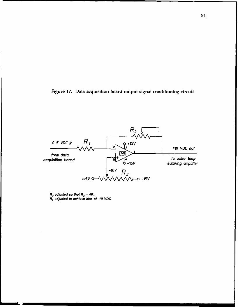
Therefore, a signal conditioning amplifier circuit that converts this 0 to 5 VDC

signal to a ±10 VDC signal was built This was done by amplifying the data

acquisition board signal by a gain of four to get a 0 to 20 VDC signal then

offsetting this with a constant -10 VDC to achieve the required ±10 VDC range

(schematic shown in Figure 17). Potentiometers were used to provide the gain

adjustment so a precisely determined signal could be achieved.

54

Figure 17. Data acquisition board output signal conditioning circuit

0-5 voc in R, +.15VS21- •k..2*7 -10 VOC out

from data F71 _

acquisition board 3 to outer loop-15V summing amplifier

-10V R 3

+15V o-- ' -15V

R2 adjusted so that R2 = 4R,R3 adjusted to achieve bias of -10 VDC

55

The method used by the data acquisition board to output a voltage is to

convert a user-definable bit count stored in a data array of between 0 and 4095

to a proportional 0 to +4.9988 VDC output signal (using -5 VDC as reference

input). This is imFortant because all software control of output voltages must be

performed in this fashion whereby the number of bits represents a proportional

voltage. Any waveform such as a continuous DC voltage or a sinusoid can be

output by the board by loading the appropriate software array with the proper

bit values. For example, a constant voltage of +1.0 VDC from the board

(equivalent to approximately -6.0 VDC once passed through the signal

conditioning amplifier) would be generated by loading several elements of an

array with an integer bit value of 819 (as calculated below)

1. 0VDC _ X4.9988VDC 4095bits

x=819.2

and commanding the software to continuously read this array and output the

appropriate voltage. This method is used several times in the orthosis control

software to bring the arm to or hold the arm at a specified angle.

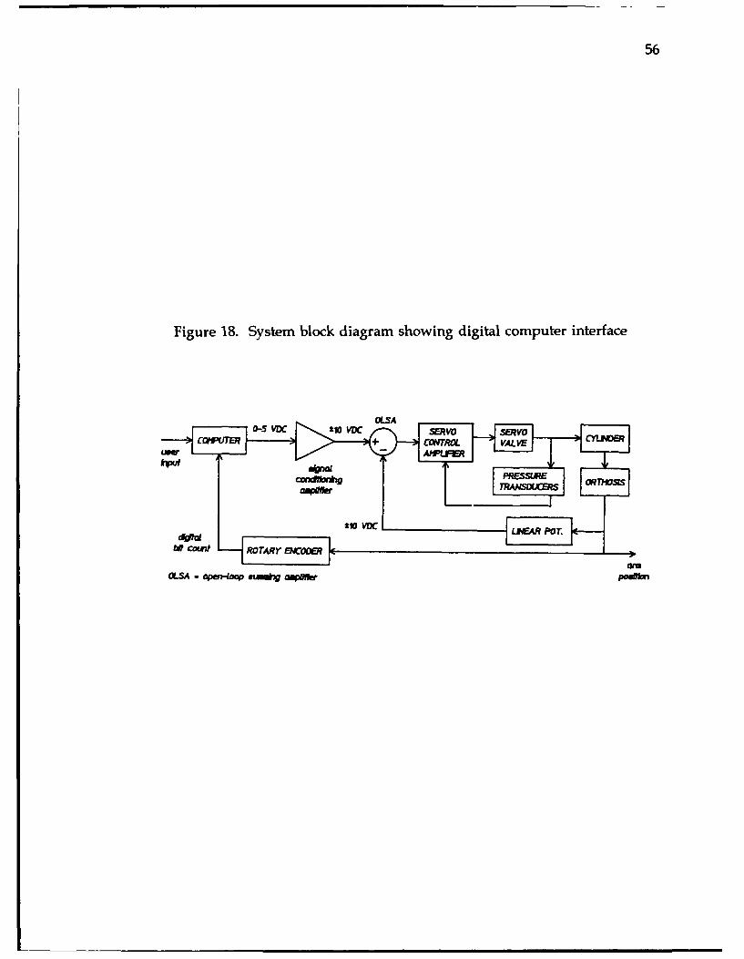
The method of position feedback control at this point is still provided by

the analog linear potentiometer signal being summed with the data acquisition

board conditioned signal at the outer loop summing amplifier (see Figure 18).

Hence, the computer is merely acti g as a cominand signal generator. In order

56

Figure 18. System block diagram showing digital computer interface

oL.A - aOpS-4Ca mu~Q pa oo

57

to provide some computer control over arm position, the pulsed signal generated

by the rotary encoder mounted on the orthosis elbow joint was sent to the

computer via a special quadrature amplifier circuit board custom built by the

department electronics technician. Although it would now be possible to use the

encoder data as position feedback instead of the linear potentiometer feedback,

time restrictions allowed me to use it merely to display the current angle of the

arm. Nevertheless, it is still important to understand the operation of the encoder

when interfaced with the computer as it has much greater potential with our

system.

The optical rotary encoder consists of a disk with 1024 small slots evenly

spaced around the circumference and infrared sensors which emit a pulse each

time one of these slots passes. The quadrature amplifier circuitry can distinguish

between pulses as well, so the actual resolution of the encoder is 2048 counts per

revolution (360 degrees), or 0.176 degree per count. The counts are accumulated

in a memory storage register so a precise value for the angular position of the

arm can be calculated by multiplying the number of counts in the register by

0.176 degree (assuming the counter was initialized at the zero degree arm position

by storing a value of zero at the initialization memory address, hex 30416).

The memory storage location for the encoder counter register requires two

bytes (eight bits per byte), allowing a bit count of up to 65,535 (2`641). The low

byte alone allows a count of up to 255 (2s-1), but since our arm will move through

an angle of about 94 degrees, this requires a count of about 532, so the high byte

58

is also needed. The low byte is available at a hex address of 30116 while the high

byte is found at hex address 30016. Software commands as found in the orthosis

control program (Appendix C-1) can be issued to read these values and use them

to find the absolute arm angle. It is necessary to point out that the encoder

increments as the arm is rotated in one direction and decrements when rotated

in the other direction. If the encoder register is initialized with a zero count and

the arm rotates in the direction that causes the encoder to decrement the count,

erroneous data results (Appendix C-2 contains a simple program that shows the

encoder register count only). This problem is encountered and corrected via

software in the orthosis control program.

By using the data acquisition board's A/D conversion ability, we have

demonstrated that the differential pressure signal available from the servo control

amplifier circuit board (at Test Point B) can be sampled and therefore used in

some manner to either aid in system control or measure any resistance the patient

may be offering, voluntarily or involuntarily (i.e., muscle spasticity). This

prospect has not been fully investigated at this point, but a strip chart example

program supplied with the data acquisition board (QBSTRIP) has allowed us to

graphically display variations in pressure as the arm is forced to move.

One final important note on hardware configuration is that the default base

address setting for the data acquisition board inside the computer is 30016 (hex),

the same address as the encoder register. Therefore, the data acquisition board's

set switches had to be changed to represent a new memory address that did not

59

conflict with the encoder or any other intrinsic computer functions (we chose hex

address 2F016 ). The INSTALL.EXE program provided with the board must be

run to create a file containing the new address location for use by the board's

own controlling software [101.

VI. SAFETY ENGINEERING

Safety of both the patient and the operator is a major concern with this

pneumatically-controlled system. Compressed air even at the 80 pounds per

square inch we are using can generate enough force to cause serious injury to

body parts in the way of moving orthosis parts. Several safety measures have

been incorporated into the orthosis hardware, but several more need to be added

before we can justifiably expect a stroke patient to use it for the first time.

The stroke of the air cylinder itself determines the maximum extension and

flexion angles, so the mechanical mounting of the cylinder on the arm provides

the mechanism by which hyperextension of the patient's arm is avoided. This

will be considered the "mechanical stops" as mentioned early in this report With

maximum rotation angles controlled, the next obvious safety concern is that the

rate at which the arm rotates be controlled. Although the orthosis control

program generates a comfortable motion profile as specified by the operator,

should a failure occur either in the software or in the electronic circuitry that

causes the servovalve to pass full flow to the cylinder, a mechanism must be in

place to keep the rotation speed to one that will not injure the patient Pneumatic

speed control valves were placed at the cylinder ports through which the flow of

air is limited according to orifice size (adjustable by thumbscrew). These speed

control valves can be set to keep the maximum rotation speed down to a safe

level, but should not restrict the air flow too greatly otherwise the system will be

overdamped and may not operate properly at normal rotation speeds.

60

61

(NOTE: These speed control valves were not installed during frequency response

testing, allowing free flow of air to the cylinder).

The orthosis control software incorporates some concern for safety but this

endeavor needs to be expanded. At the start of the program when the arm must

swing from one extreme point to the other, the software displays a red warning

screen and waits for a key press from the operator to ensure nobody is near (or

strapped in). Also, during operation of the arm, the operator is reminded that at

any time any key on the keyboard may be pressed to stop motion if required.

VII. IDEAS FOR FURTHER IMPROVEMENT

This section lists both suggestions that should be incorporated as soon as

practical and ideas which may in the future contribute to the efficient operation

of the system. They are broken down into four categories: Hardware

modifications, control system challenges, software improvements, and safety

additions.

HARDWARE

1. An effective mounting platform needs to be developed that will easily

allow the operator to fasten the orthosis to the patient in the wheelchair (in

work).

2. The cylinder mounting position should be altered so as to move the

available 94 degree range of motion from a starting angle of 0 degrees to

one of about 25 to 30 degrees so that the maximum flexion angle becomes

about 120 degrees or 130 degrees (suggested by Dr. Lieber-patient would

then be moving arm at an angle that, once rehabilitated, allows easy access

to the mouth area).

3. It should be fairly easy to disconnect the pneumatic cylinder from the

orthosis and install a DC servomotor which can be controlled by the

existing system components. This might provide useful information

should this alternative be more desirable at a later date.

4. The incorporation of a mechanism which attaches to the existing orthosis

structure and provides wrist flexion and extension as the arm is operating

62

63

would be fairly easy to incorporate and could prove to be a great benefit

in patient rehabilitation.

CONTROL SYSTEM

1. Operation of the "percent assist" mode may require temporary removal of

position feedback from the system so that it operates under pressure

control only. This can be done most efficiently by rewiring the linear

potentiometer feedback from the outer loop summing amplifier to the data

acquisition board (as an analog input to be digitally converted) where it

would be summed with the software-generated command signal in normal

operation or ignored while in this mode. The system should compensate

if the patient were to add more force than necessary to put the orthosis in

motion at the selected assist percentage (thus causing an acceleration and

increase in velocity) by reducing the degree of assist in an attempt to

maintain a constant arm velocity.

2. An improvement to the aesthetic appearance of the orthosis could be

achieved by removing the linear potentiometer, which then dictates that

the system would receive position feedback solely from the optical rotary

encoder. This should be feasible with proper software development

3. Addition of integral or derivative control techniques to improve system

performance might be interesting. The servo control amplifier circuit

board has provisions for such rate compensation.

64

4. Adjustment of the gain potentiometers throughout the circuitry may yield

a better combination of system gains which could improve performance.

SOFITWARE

1. The user interface should be tested by several potential operators and their

suggestions incorporated.

2. Programs written in BASIC should be compiled using a BASIC compiler

or converted to another language to significantly increase processing speed.

3. A module should be written to take the sampled pressure transducer

difference signal and use it to determine patient strength during the static

evaluation mode or measure muscle spasticity during the passive exercise

mode.

4. The existing orthosis control program should be upgraded to include the

ability to perform the patient's initial range of motion calibration without

pneumatic assistance. The therapist would move the orthosis/ patient arm

to a maximum desired extension angle then press a key to store that angle

(available from the encoder register) and do the same for the maximum

desired flexion angle. Pneumatic assistance could then be applied at this

point.

5. Real time graphical display of selected parameters should be an option.

Incorporate the example program "QBSTRIP" to get real-time display of

pressure difference for use in the static evaluation mode.

65

6. A master control program should be developed that contains a patient

database and stores information in files from all previous patient tests. It

should also be able to graphically display a progress history and output

relative quantitative values for study (i.e., strength, power, energy, etc.).

It should also allow selection of the various test modes.

7. Code should be written to generate periodic interrupts (from the data

acquisition board) at a preselected time interval which would fetch the

value in the encoder register. Using algorithms currently being developed

and tested, these periodic encoder counts can be used to determine angular

velocity and acceleration of the arm which would then be used in the

calculation of power and energy. These calculations will be required in the

dynamic evaluation mode.

SAFETY

1. Areas on the orthosis which could crush the hand and/or fingers during

operation should be covered with some sort of rubber, plastic or cloth boot.

Such areas include the area directly above the elbow joint and underneath

the piston rod mounting bracket.

2. In order to regulate supply pressure at a constant predetermined value, the

electro-pneumatic regulator (donated by SMC Corporation) could be used

and, in fact, controlled via computer if pressure changes were desired (i.e.,

to unstrap patient, to allow therapist to move orthosis/patient arm, etc.).

Also, an electrically-operated bi-directional valve (also from SMC) could

66

be placed in the air circuit that would :equire a constant voltage for air to

flow to the system so that any power failure or operator-initiated

emergency stop sequence would protect the patient arm from sudden

movements.

3. Any controlling software needs to be thoroughly tested to ensure certain

actions or keystroke combinations do not result in the sudden,

uncontrolled movement of the arm. The current version of the orthosis

control program does have these problems under certain conditions when

using the cursor positioning controls.

VIII. CONCLUSION

We have seen that pneumatics is a viable option for powering our orthosis

by providing smooth, precise control of arm position and that our configuration

has the capability to command the arm in several different modes of operation.

Much work has been done to bring the robotic arm to this stage of development,

but much more remains to continue developing ways in which it can be more

useful to the people who will be operating it and hopefully more beneficial to the

patients who may eventually use it as part of their rehabilitation program.

67

APPENDIX A

EXPERIMENTAL FREQUENCY RESPONSE PLOTS

A-i: Closed-Loop System with Pressure and Position FeedbackA-2: Open-Loop Position MeasurementA-3: Open-Loop Pressure Measurement

68

69

t---

H ! i

70

8- - - - -- -

3 -F .~-------:-j :1 ______----------__

-~~~~ ~ .- -. .. .- .__.__.__.__.

77 - - - - --- - -___--__

_ _ _r 7,_~

71

A--

I 4I ,

13,

ýj.e ýL-,arthmhc Ce ¶ T The I,Ch

APPENDIX B

ROOT LOCUS ANALYSES OF EXPERIMENTALLY-DERIVED SYSTEM TRANSFER FUNCTIONS

B-I: Position Feedback OnlyB-2. Position and Pressure Feedback

72

APPENDIX B-1

ROOT LOCUS ANALYSIS(POSITION FEEDBACK ONLY)

The open-loop transfer function (OLTF) for this system is:

G(s) = 31158.68s(s+22) (s+37.7)

Origin of asymptote crossing = (37.7 + 22)/3 = 59.7/3 = 19.9

Using the magnitude criterion with test points along negative real axis to findlocus breakaway point (point of relative maximum magnitude),

IG(s) J= Is('js+22"1s+37.7j

31158.68

which is a maximum of 0.11 at a test point of s=-9.

Finding where the locus crosses the imaginary axis:

1+G(s) H(s) =0

I+ 31158.68.K =0s (s+22) (s+37.7)

The characteristic equation of the above transfer function is

S3+59.7s2+829.4s+31158.68K=0

and substituting s=jto then equating the imaginary terms to zero yields

co=±28.8

for the imaginary axis crossing point Setting the real terms to zero results in again factor K=1.59 at which the closed-loop poles will lie on the axis and thesystem becomes unstable (a system gain of 49,542.3). Because K is greater thanone the closed-loop poles are in the left-half plane and our system is thus stable.

73

74

We can also use the characteristic equation to find the location of the system'sclosed-loop poles in its current state (K=1, or a system gain of 31,158.68). Theseroots, and hence pole locations, are

s=-54.93

s=-2.385±23.7j

and are shown on the accompanying root locus diagram along with the originalopen-loop poles.

gain=49,542.330

STABLE gain=31,158.68 UNSTABLEREGION REGION

-20

asymptote -

-10

* open-loop pole

* closed-loop pole

APPENDIX B-2

ROOT LOCUS ANALYSIS(POSITION AND PRESSURE FEEDBACK)

The open-loop transfer function (OLTF) for this system is:

G(s) = 31158.68s(s+22) (s+57.58)

Origin of asymptote crossing = (57.58 + 22)/3 = 79.58/3 = 26.53

Using the magnitude criterion with test points along negative real axis to findlocus breakaway point (point of relative maximum magnitude),

IG(s) J= Is1"1s+221"1s+57.581

31158.68

which is a maximum of 0.1832 at a test point of s=-10.

Finding where the locus crosses the imaginary axis:

1+G(s) H(s) =0

1+ 31158.68-K =0s(s+22) (s+57.58)

The characteristic equation of the above transfer function is

s3 +79 .58s 2 +1266.76s+31158.68K=0

and substituting s=j(o then equating the imaginary terms to zero yields

w=±35.59

for the imaginary axis crossing point Setting the real terms to zero results in again factor K=3.24 (system gain of 100,954.1) at which the closed-loop poles willlie on the axis and the system becomes unstable. Because K is greater than onethe closed-loop poles are in the left-half plane and our system is thus stable.

75

76

We can also use the characteristic equation to find the location of the system'sclosed-loop poles in its current state (K=1, or a system gain of 31,158.68). Theseroots, and hence pole locations, are

s=-67.66

s=-5.96±20.61j

and are shown on the accompanying root locus diagram along with the originalopen-loop poles.

gain= 100.954.1

35

-30

STABLE 2 UNSTABLEREGION gain=31,158.6 REGION

20

'S

asymptote

j5 t A5 J.0 -t -. .1, 15 5 .

* open-loop pole

* closed-loop pole-20

*25

-35

APPENDIX C

SOFTWARE LISTINGS AND DESCRIPTIONS

C-1: Orthosis Control ProgramC-2. Simple Encoder Testing Program

77

APPENDIX C-1

ORTHOSIS CONTROL PROGRAM(ROBOTARM.BAS)

This program, written in BASIC, is the controlling program for the only

functional mode of orthosis operation, the passive exercise mode. It was built

upon an example program supplied with the data acquisition board (EX18.BAS)

which allows voltage output of various waveforms based on values loaded into

an array.

The program interacts with the operator by first showing a red warning

screen to make sure operator and patient are clear of the orthosis while it gets

initialized. When the <ENTER> key is pressed, the software commands the data

acquisition board to generate a null output (which is 0 VDC but becomes -10 VDC

because of the signal conditioning amplifier) which, because of the linear

potentiometer position feedback, causes the orthosis to swing to its fully extended

position. Here, the encoder register is initialized to zero counts so that absolute

angle information as the arm is moving can be obtained. The software then

commands the board to output its full scale voltage (a bit value of 4095 equivalent

to +4.9988 VDC, but after the signal conditioning amplifier becomes +10 VDC)

which swings the arm to its full flexion position where the encoder register is

read to determine the maximum angle the arm has moved. The operator is now

prompted to use the cursor keys to move the arm down to a more comfortable

angle for patient attachment if desired. Once tLie patient is ready, the operator

is then prompted to again use the cursor keys to move the arm up or down to

78

79

enter the maximum desired flexion angle for the therapy session. Once this value

is recorded, the operator is prompted to move the arm down to the maximum

desired extension angle to be used (according to patient comfort). The

opportunity to enter a rest period at each extreme position is available, then the

number of exercise cycles is requested (one cycle is motion of the orthosis from

maximum extension angle to maximum flexion angle back to maximum extension

angle). If "0" is entered, the profile will continue operation until commanded to

stop by pressing any key. Next, the desired rotational velocity is requested and

the software then calculates the output data array elements based on the entered

parameters. These elements will produce a triangle wave (clipped if any rest time

is selected) with a frequency and magnitude dependent on these entered

parameters. When this calculation is complete, the operator is told that the

exercise will begin when any key is pressed. The data acquisition board uses the

data array elements to output proportional voltages which cause the arm to move

though the desired motion profile. The time remaining for the exercise is

displayed if other than continuous operation was selected. When complete, the

operator has the option of repeating the exact same motion profile or cycling back

to the point in the program where new parameters can be entered.

Detailed software control of the data acquisition board is outlined in the

operations manual [10], but basically the board receives its commands through

information passed to it via a pre-compiled binary subroutine called DAS16. The

call to this subroutine within the BASIC program must always contain an integer

80

variable (representing the desired mode number), an integer array (containing

information about how that mode is to be operated), and another integer variable

(a returned value representing any error conditions). Although there are over 20

modes of operation for the data acquisition board, I will only describe the four

used in this program.

Mode 0 is merely an initialization which should be run before using any

of the other modes, otherwise the board will default to specified parameters.

Mode 7 is used to terminate any outputs from the board and should be

used before any call to Mode 18.

Mode 18 outputs a voltage based on integer elements between 0 and 4095

stored in an array. If Mode 18 is called while the board is outputting any other

signal, erroneous signals will be produced and the servovalve will start "buzzing"

loudly.

Mode 17 is used to set the rate at which elements of the desired output

signal data array are to be converted to their appropriate output voltages. This

mode uses the integer product of the frequencies set for two independent timers

to create the desired output sampling frequency.

When performing other operations such as sampling an incoming analog

signal (i.e., the pressure transducer difference signal), access to different modes

will be required.

The latest version of the orthosis control program, called ARMCONTROL,

is listed on the following pages.

81

10 ' ************** ***** ** ****** **** ** **** ***** **** *** *****w** **** ********

20 '* PROGRAM: ARMCONTROL *

30 '* INITIALIZES ARM, ALLOWS CURSOR CONTROL OF MOTION, REQUESTS *

40 * PARAMETERS FOR EXERCISE MOTION PROFILE, AND PERFORMS PASSIVE *

50 * EXERCISE MODE. *

60 ********************************************************************

70

80 ' --------- STEP 1----------------------------------------------

90 'First load DAS16.BIN routine by contracting BASIC to 48K workspace

100 CLEAR, 49152! 'reduce workspace to 48K

110 DEF SEG 0 'find BASIC's segment

120 SG = 256 * PEEK(&H511) + PEEK(&H510)

130 SG = SG + 49152!/16 'the ! denotes a single precision value

140 DEF SEG = SG 'SG = load location for

150 BLOAD "DAS16.BIN", 0 'DAS16.BIN routine

160

170 '--------- STEP 2----------------------------------------------

180 'Initialize data acquisition board using mode 0

190 DIM D%(15) 'declare integer (%) data array

200 'Find the board's base address from DAS16.ADR file (run INSTALL.EXE to

210 'generate this file if any changes have been made to the configuration).

220 'The default base address of hex 300 cannot be used in our system because

230 'the encoder's quadrature amplifier board built by Tom Phillips occupies

240 'that address. We are using a base address of hex 2FO or decimal 752.

250 OPEN "DAS16.ADR" FOR INPUT AS #1 : INPUT #1, D%(O) : CLOSE #1

260 D%(1) = 2 'interrupt level

270 D%(2) = 1 'D.M.A. level

280 'Be sure that base address & DMA level correspond to switches

290 'on DAS-16F!

300 MD% = O 'initialize mode

310 FLAG% = 0 'declare error variable

320 DAS16 = 0 'CALL offset = 0

330 CALL DAS16 (MD%,D%(0),FLAG%) 'initialize

340 'Check for any initializing errors

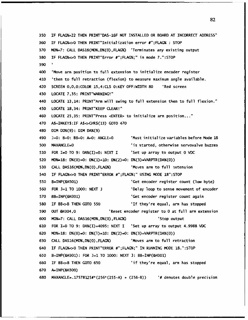
82

350 IF FLAG%=22 THEN PRINT"DAS-16F NOT INSTALLED OR BOARD AT INCORRECT ADDRESS"

360 IF FLAG%<>O THEN PRINT"Initialization error #";FLAG% : STOP

370 MD%=7: CALL DAS16(MD%,D%(O),FLAG%) 'Terminates any existing output

380 IF FLAG%<>O THEN PRINT"Error #";FLAG%;" in mode 7.":STOP

390

400 'Move arm position to full extension to initialize encoder register

410 'then to full retraction (flexion) to measure maximum angle available.

420 SCREEN 0,O,0:COLOR 15,4:CLS O:KEY OFF:WIDTH 80 'Red screen

430 LOCATE 7,35: PRINT"WARNING!"

440 LOCATE 13,14: PRINT"Arm will swing to full extension then to full flexion."

450 LOCATE 18,34: PRINT"KEEP CLEAR!"

460 LOCATE 25,35: PRINT"Press <ENTER> to initialize arm position..."

470 A$=INKEYS:IF AS<>CHRS(13) GOTO 470

480 DIM DD%(9): DIM DA%(9)

490 J=0: B=O: BB=O: A=O: ANGLE=O 'Must initialize variables before Mode 18

500 MAXANGLE=O 'is started, otherwise servovalve buzzes

510 FOR I=0 TO 9: DA%(I)=O: NEXT I 'Set up array to output 0 VDC

520 MD%=18: D%(O)=O: D%(1)=10: D%(2)--0: D%(3)=VARPTR(DA%(0))

530 CALL DAS16(MD%,D%(O),FLAG%) 'Moves arm to full .xtension

540 IF FLAG%<>O THEN PRINT"ERROR #";FLAG%;" USING MODE 18":STOP

550 B=INP(&H301) 'Get encoder register count (low byte)

560 FOR J=1 TO 1000: NEXT J 'Delay loop to sense movement of encoder

570 BB=INP(&H301) 'Get encoder register count again

580 IF BB<>B THEN GOTO 550 'If they're equal, arm has stopped

590 OUT &H304,0 'Reset encoder register to 0 at full arm extension

600 MD%=7: CALL DAS16(MD%,D%(O),FLAG%) 'Stop output

610 FOR I=0 TO 9: DA%(I)=4095: NEXT I 'Set up array to output 4.9988 VDC

620 MD%=18: D%(O)=O: D%(1)=10: 0%(2)--0: D%(3)=VARPTR(DA%(O))

630 CALL DAS16(MD%,D%(O),FLAG%) 'Moves arm to full retraction

640 IF FLAG%<>O THEN PRINT"ERROR #";FLACG;" IN RUNNING MODE 18.":STOP

650 B=INP(&H301): FOR J=1 TO 1000: NEXT J: BB=INP(&H301)

660 IF BBo'B THEN GOTO 650 'if they're equal, arm has stopped

670 A=INP(&H300)

680 MAXANGLE=.17578125#*(256*(255-A) + (256-B)) '# denotes double precision

83

690 MD%=7: CALL DAS16(MD%,E'Y(O),FLAG%) 'Stop output

700

710 'Now enable cursor control of arm

720

730 SCREEN O,0,O:COLOR 14,1:CLS O:KEY OFF:WIDTH 80

740 PS%=4095 'initialize integer variable PS to eflect current position in

750 'full flexion.

760 COLOR 7: LOCATE 7,19: PRINT"USE UP AND DOWN CURSOR KEYS TO MOVE ARM TO"

770 COLOR 15: LOCATE 9,22: PRINT"DESIRED ANGLE FOR PATIENT ATTACHMENT"

780 GOSUB 1860 'Performs cursor control and angle readout

790 CLS 0: COLOR 7

800 LOCATE 7,19: PRINT"USE UP ,A':D DOWN CURSOR KEYS TO MOVE ARM TO"

810 COLOR 15: LOCATE 9,29: PRINT"MAXIMUM FLEXION ANGLE"

820 GOSUB 1860

830 MAX=PS% 'set MAX to voltage level determined by PS

840 CLS 0: COLOR 7

850 LOCATE 7,19: PRINT"USE UP AND DOWN CURSOR KEYS TO MOVE ARM TO"

860 COLOR 15: LOCATE 9,29: PRINT"MAX2[MUM EXTENSION ANGLE"

870 GOSUB 1860

880 MIN=PS% 'set MIN to voltage level determined by PS

890 1

900 'Get user-desired exercise parameters

910 '

920 CLS 0: COLOR 15: LOCATE 7,25

930 PRINT"Enter rest time at each end"

940 LOCATE 9,25: INPUT"(O-15 seconds)";DELAY

950 IF DELAY<O OR DELAY>15 THEN GOTO 920

960 CLS 0: COLOR 15: LOCATE 7,18

970 PRINT"Enter number of exercise cycles to perform"

980 LOCATE 9,18: INPUT"(1-100 or 0 for continuous)";CYCLES

990 IF CYCLES<O OR CYCLES>100 THEN GOTO 960

1000 CLS 0: COLOR 15: LOCATE 7,20

1010 PRINT"Enter desired rotation velocity"

1020 LOCATE 9,20: INPUT"(1-90 deg/sec)";RATE

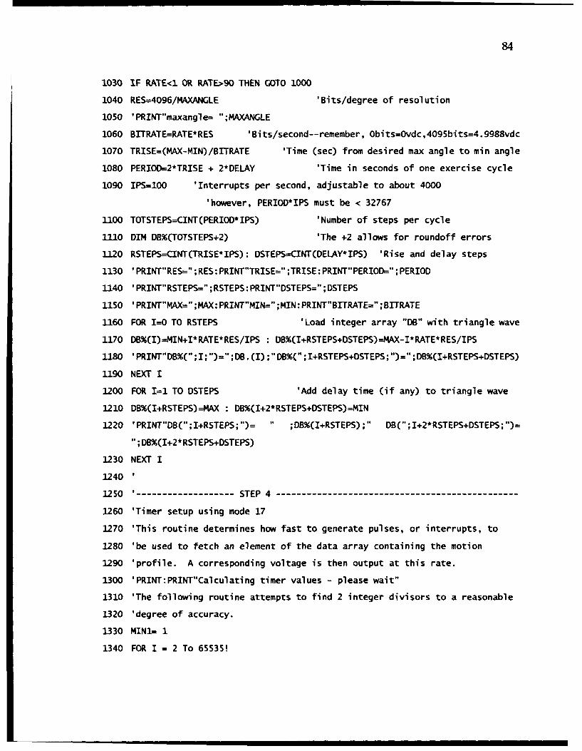
84

1030 IF RATE<1 OR RATE>90 THEN GOTO 1000

1040 RES=4096/MAXANGLE 'Bits/degree of resolution

1050 'PRINT"maxangle= ";MAXANGLE

1060 BITRATE=RATE*RES 'Bits/second--remember, Obits=Ovdc,4095bits=4.9988vdc

1070 TRISE=(MAX-MIN)/BITRATE 'Time (sec) from desired max angle to min angle

1080 PERIOD=2*TRISE + 2*DELAY 'Time in seconds of one exercise cycle

1090 IPS=100 'Interrupts per second, adjustable to about 4000

'however, PERIOD*IPS must be < 32767

3100 TOTSTEPS=CINT(PERIOD*IPS) 'Number of steps per cycle

1110 DIM DB%(TOTSTEPS+2) 'The +2 allows for roundoff errors

1120 RSTEPS--CINT(TRISE*IPS): DSTEPS--CINT(DELAY*IPS) 'Rise and delay steps

1130 'PRINT"RES-=" ; RES: PRINT"TRISE=" ;TRISE: PRINT"PERIOD=" ; PERIOD

1140 'PRINT"RSTEPS=" ; RSTEPS: PRINT"DSTEPS=" ; DSTEPS

1150 'PRINT"MAX=" ; MAX: PRINT"MIN=" ; MIN: PRINT"BITRATE=" ; BITRATE

1160 FOR 1--0 TO RSTEPS 'Load integer array "DB" with triangle wave

1170 DB%(I)--MIN+I*RATE*RES/IPS : DB%(I+RSTEPS+DSTEPS)--MAX-I*RATE*RES/IPS

1180 'PRINT"DB%(" ; I; ")="; DB. (I) ; "DB%("; I+RSTEPS+DSTEPS; ")=" ; DB%(I+RSTEPS+DSTEPS)

1190 NEXT I

1200 FOR I=1 TO DSTEPS 'Add delay time (if any) to triangle wave

1210 DB%(I+RSTEPS)=MAX : DB%(I+2*RSTEPS+DSTEPS)--MIN

1220 'PRINT"DB(';I+RSTEPS; ")= ;DB%(I+RSTEPS);" DB(" ;I+2*RSTEPS+DSTEPS; ")=

"; DB%(I+2*RSTEPS+DSTEPS)

1230 NEXT I

1240 '

1250 '------------------- STEP 4----------------------------------------------

1260 'Timer setup using mode 17

1270 'This routine determines how fast to generate pulses, or interrupts, to

1280 'be used to fetch an element of the data array containing the motion

1290 'profile. A corresponding voltage is then output at this rate.

1300 'PRINT'PRINT"Calculating timer values - please wait"

1310 'The following routine attempts to find 2 integer divisors to a reasonable

1320 'degree of accuracy.

1330 MINI= 1

1340 FOR I = 2 To 65535!

85

1350 RESl= 1000000!/(I*IPS)

1360 RES1= ABS(RES1- CINT(RES1))

1370 IF RES1< MINI THEN MINI = RESI:N1 = I:N2=CINT(1000000!/(IPS*N1))

1380 IF MINI < .01 THEN I = 65536!

1390 NEXT 1

1400 'LOCATE CSRLIN-l, 1: PRINT SPC(79):PRINT"Actual output rate will be";1 000000!/(N1*N2*TOTSTEPS);" cycles/sec."

1410 MD% = 17

1420 IF Ni > 32767 THEN Ni = NI - 65536!

1430 D%(O) = Ni

1440 IF N2 > 32767 THEN N2 = N2 - 65536!

1450 D%(1) = N2

1460 CALL DASG (MD%, D%(O), FLAC%)

1470 IF FLAGo<0 THEN PRINT"Error #";FLAG%;" in setting timer rate":STOP

1480 'You can load any other waveshape you li~'e, 0 = 0 volts, 4095 = 4.9988 volts

1490 '

1500 ' --------- STEP 7----------------------------------------------

1510 'Ready to begin - prompt user for start

1520 COLOR 14: LOCATE 15,20: PRINT"Press any key to start exercise"

1530 IF INKEY$=."" GOTO 1530

1540 DURATION=O: MINUTES1=0: MINUTES2=0: SECONDSI-=0: SECONDS2--0

1550 '

1560 ' --------- STEP 8----------------------------------------------

1570 'Note: Start of mode 18 can be held off in hardware by keeping IPO

1580 ' low until ready.

1590

1600 MD% = 18

1610 D%(O) = 0

1620 D%(1) = TOTSTEPS

1630 D%(2) = CYCLES

1640 D%(3) = VARPTR(DC%(O))

1650 CALL DASG (MD%, D%(O), FLAG%)

1660 IF FLAG%<>O THEN PRINT"Error #";FLAG%;" in running mode 18":STOP

1670 CLS 0

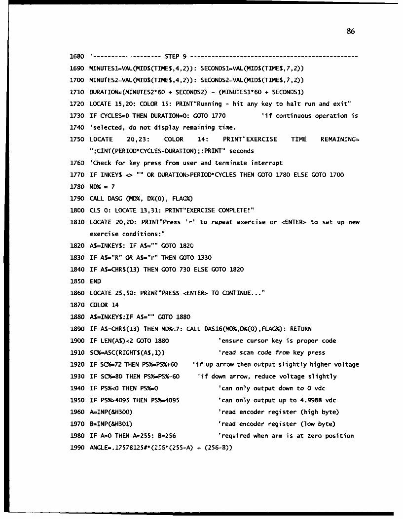
86

1680 '---- STEP 9

1690 MINUTES1=VAL(MIDS(TIME$,4,2)): SECONDS1=VAL(MIDS(TIME$, 7,2))

1700 MINUTES2=VAL(MID$(TIMES, 4,2)): SECONDS2=VAL(MIDS(TIMES, 7,2))

1710 DURATION=(MINUTES2*60 + SECONDS2) - (MINUTES1*60 + SECONDS1)

1720 LOCATE 15,20: COLOR 15: PRINT"Running - hit any key to halt run and exit"

1730 IF CYCLES=O THEN DURATION=0: GOTO 1770 'if continuous operation is

1740 'selected, do not display remaining time.

1750 LOCATE 20,23: COLOR 14: PRINT"EXERCISE TIME REMAINING=";CINT(PERIOD*CYCLES-DURATION) ; :PRINT" seconds

1760 'Check for key press from user and terminate interrupt

1770 IF INKEYS o ."" OR DURATION>PERIOD*CYCLES THEN GOTO 1780 ELSE GOTO 1700

1780 MD% = 7

1790 CALL DASG (MD%, D%(O), FLAG%)

1800 CLS 0: LOCATE 13,31: PRINT"EXERCISE COMPLETE!"

1810 LOCATE 20,20: PRINT"Press 'r' to repeat exercise or <ENTER> to set up new

exercise conditions:"

1820 AS=INKEYS: IF AS="" GOTO 1820

1830 IF AS="R" OR AS="r" THEN GOTO 1330

1840 IF A$---CHRS(13) THEN GOTO 730 ELSE GOTO 1820

1850 END

1860 LOCATE 25,50: PRINT"PRESS <ENTER> TO CONTINUE..."

1870 COLOR 14

1880 AS=INKEYS:IF AS=-"" GOTO 1880

1890 IF AS=CHRS(13) THEN MD%=7: CALL DAS16(MD%,D%(O),FLAG%): RETURN

1900 IF LEN(AS)<2 GOTO 1880 'ensure cursor key is proper code

1910 SCY-A5C(RIGHTS(AS,1)) 'read scan code from key press

1920 IF SC%=72 THEN PS%=PS%+60 'if up arrow then output slightly higher voltage

1930 IF S06=80 THEN PS%=PS%-60 'if down arrow, reduce voltage slightly

1940 IF PS%<O THEN PS%=O 'can only output down to 0 vdc

1950 IF PS%>4095 THEN PS%=4095 'can only output up to 4.9988 vdc

1960 A-INP(&IH300) 'read encoder register (high byte)

1970 B-INP(&H301) 'read encoder register (low byte)

1980 IF AMO THEN A=255: B=256 'required when arm is at zero position

1990 ANGLE=.17578125#*(2=5*(255-A) + (256-8))

87

2000 'The encoder decrements from extension to flexion.

2010 LOCATE 13,27: PRINT USING"ARM ANGLE = ###.## DEGREES";ANGLE

2020 FOR I=0 TO 9: DD%(I)=PS%: NEXT I

2030 MD%=7: CALL DAS16(MD%,D%(O),FLAG%) 'terminate any output before MODE 18

2040 MDX=18: D%(O)=0: D%(1)=10: D%(2)=O: D%(3)=VARPTR(DD%(O))

2050 CALL DAS16(MD%,D%(O),FLAG%) 'move arm to new position

2060 IF FLAG%<>O THEN PRINT"ERROR #";FLAG*;" IN RUNNING MODE 18":STOP

2070 GOTO 1880 'be ready to accept any more key inputs

APPENDIX C-2

SIMPLE ENCODER TESTING PROGRAM(ENCODER.BAS)

This program sets the rotary encoder's initialization memory storage register

to a count of zero when the program is started (the arm should be fully extended

otherwise erroneous data will result). It is then put into a loop which

continuously reads the encoder register's low and high bytes used to determine

and display the current arm angle. The double precision value 0.17578125 is the

exact resolution of the encoder in degrees/count. This value is multiplied by the

number of counts to produce the arm angle. If the encoder were wired so that

it incremented as the arm moved up, line 40 would read

40 ANGLE = 0.17578125#*(256*A + B)

but since it decrements in that direction and since an angle of 0 degrees is defined

to be at full extension, the correction found in the program's line 40 (and in the

orthosis control program) was necessary to simulate incrementing the counter as

the arm rotated up. The BASIC program is listed on the following page.

88

89

BASIC Program Listing for Testing Rotary Encoder Operation

10 'RUN THIS PROGRAM WHEN ARM IS FULLY EXTENDED

20 OUT &H304,0

30 COLOR 14,1

40 KEY OFF

50 CLS 0

60 A=INP(&H300)

70 B=INP(&H301)

80 IF A=O THEN A=255:B=256

90 ANGLE=.1757812S#*(2S6*(255-A) + (256-B))

100 IF ANGLE < 0 THEN ANGLE = 0!

130 LOCATE 13,30

120 PRINT USING "ARM ANGLE = ###.## DEGREES" ;ANGLE

130 GOTO 60

140 END

REFERENCES

[1] Vernon L. Nickel, M.D., M.Sc., retired Professor of Surgery for theUniversity of California, San Diego Medical School (Orthopedics andRehabilitation) and Director of Rehabilitation at the Sharp Rehabilitation Centerin San Diego.

[2] Isaka, S., Schneider, A., Filia, P., Lue, K, Coutts, R., Nickel, V., "A New Toolfor Stroke Rehabilitation Study," proceedings of RESNA 10th Annual Conference,San Jose, CA, 1987.

[3] Blevins, F., Coutts, R., Lieber, R., Schneider, A., Guier, C., Rosenstein, A.,Stewart, W., Filia, P., Nickel, V., "The Effect of Patterning Using ContinuousPassive Motion on Stroke Rehabilitation," proceedings of 34th Annual Meeting,U~rthopaedic Research Society, February 1-4, 1988, Atlanta, Georgia.

[4] S. Gordon, "Servo Control of Pneumatic Systems Is Here," Hydraulics &Pneumatics, July 1991.

[5] deSilva, Clarence W., Control Sensors and Actuators. Prentice Hall, 1989.

[6] Richard Duder, Vice President of Engineering, Dynamic Valves,Incorporated, 923 Industrial Avenue, Palo Alto, CA 94303. Phone: (800) 227-8825.

[7] Operations manual for Model 23-7030A Servovalve Control Amplifier,Dynamic Valves, Inc.

[8] Ogata, Katsohiko, Modern Control Engineerin& second edition, PrenticeHall, 1990.

[9] McCloy, D. and H.R. Martin, The Control of Fluid Power. John Wiley &Sons, 1973.

[101 Operations manual for Keithley-Metrabyte DAS-16F Data Acquisition Board.

[111 Reference manual for the GW BASIC programming language, AT&T andMicrosoft, Inc., 1984.

90