Representations of Geometry for Computer Graphics

Course 29 Tuesday / Full Day / Advanced

The latest research on the most important computational representations ofgeometry used in computer graphics. The emphasis is on their strengths andweaknesses and how to build a coherent system that supports multiplerepresentations.

Schedule & Table of Contents

8:30 am: Introduction to Computational Representations of Geometry - Naylor Course objectives and taxonomy of representations.

8:45 am: Voxels as Computational Representations of Geometry - Kaufman Volume graphics is an emerging subfield of computer graphics concerned with the synthesis, manipulation, and rendering of volumetric modeled objects, stored as a volume buffer of voxels. Unlike volume visualization which focuses primarily on sampled and computed data sets, volume graphics is concerned primarily with modeled geometric scenes and particularly with those that are represented in a regular volume buffer. Volume graphics has advantages over surface graphics by being viewpoint independent, insensitive to scene and object complexity, and suitable for the representation of sampled and simulated data sets and mixtures thereof with geometric objects. It supports the visualization of internal structures, and lends itself to the realization of block operations, CSG modeling, and hierarchical multi-resolution representations. The problems associated with the volume buffer representation, such as discreteness, memory size, processing time, and loss of geometric representation, echo problems encountered when raster graphics emerged as an alternative technology to vector graphics and can be alleviated in similar ways.

10:00 am: Break

10:15 am: - Specification, Representation, and Construction of Non-ManifoldeGeometric Structures - Rossignac

We will discuss boundary/topological representations for characterizing the topological coverages of CAD system, for comparing the data structures they maintain, and for reliably computing boundary models from constructive representations. Creating multi-resolution representation will be addressed.

11:15 am: Modeling with Simplicial Complexes - Edelsbrunner The main theme of this talk is the idea of using cell decompositions (complexes) to model geometric shapes. The complex is what is often called a grid or mesh. This approach to modeling allows the instantaneous analysis of the created shape. The following specific questions and issues will be addressed.

• What are complexes? (definitions and examples)• How can the geometric integrity of a complex be guaranteed?• How can complexes be used to model shape?• How can complexes be manipulated and maintained?

12:00 noon: Break

1:30 pm: Polynomial Surface-Patch Representations - Bajaj Algebraic curves and surfaces can be represented in an implicit form, and sometimes also in a parametric form. We will compare the implicit and parametric representations of algebraic surfaces by considering the the parametric form either as a mapping or alternatively, an algebraic variety. In this course, I shall consider specific geometric operations: scattered data fitting and surface display and compare the implicit and parametric forms for their superiority (or lack thereof) in optimizing algorithms for these operations.

3:00 pm: Break

3:15 pm: Binary Space Partitioning Trees - Naylor Partitioning Trees, a multi-dimensional generalization of binary search trees, provide a computational representation of geometry via recursive subdivision with hyperplanes defined by linear equations. Linearity and recursive subdivision lead to simple algorithms for visibility (hidden surface removal, transparency, shadows) as well as intersections (set operations, collision detection, clipping, ray-tracing). We will present a review of these capabilities as well as present new results on building multi-resolution trees, representing volumetric data, and integrating parametric surfaces into Partitioning Trees to permit local non-linear deformations.

4:15 pm: Building a Whole Geometry System - All

Having presented each of the representational schemes, we will now be in a position to focus exclusively on the relation between the various representations and how one can build a single coherent geometry system that exploits the strengths of each and avoids their weaknesses. We will be able to draw upon the experience of several of the speakers who have built such integrated systems.

1

Computational Representationsof Geometry

Bruce NaylorSpatial Labs Inc.

I n t r o d u c t i o n

Computational representations of geometry provide the foundations for all the various a r e a sof computing that involve geometry. These areas currently include Computer Graphics,Computer-Aided Geometric Design, Scientific Visualization, Computational Geometry, FiniteElement Analysis, Robotics, Computer Vision and Image Processing. Yet only a fewrepresentations of geometry have emerged to date. We believe that the reason for this is t h a tgeometric sets are describable in terms of only a few fundamental aspects, e.g. their topology,or set theoretic structure, etc. Many of the representations, in their purest form, describeprimarily a single fundamental aspect of geometric sets. Each "pure" representation then isthe language for expressing that aspect (it is the syntatic form for which the in tendedsemantic interpretation is direct). For example, the topology of a set is expressed directly a n dexactly by what we naturally call "a topological representation": a graph with a one- to -onecorrespondence between graph nodes and topologically connected components, and w h e r egraph edges indicate incidence between components. In addition to pure representat ions ,other types of representations may be hybrids, combining multiple aspects simultaneously.

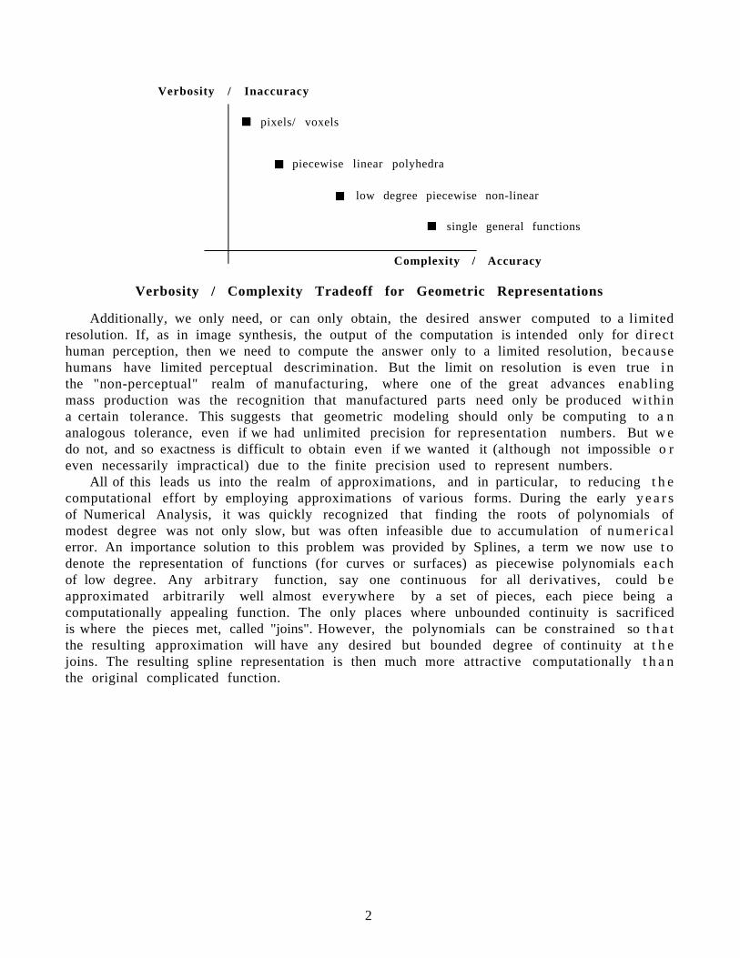
Representatons of geometry have a very strong connection to "traditional" mathematics,both historically, dating back to Classical Greek civilization, and to modern subjects. Theseinclude Set Theory, Graph Theory, Algebraic Topology, etc., in addition to the var iousvarieties of Geometry: Projective, Analytic, Algebraic, Differential, and Combinatorial. Whatis different, as everyone knows, is that computation is "constructive mathematics", and t h eprimary measure of value is not proveability per se (as much as we might want error f r eeprograms), but rather performance and accuracy. The pursuit of efficiency has lednumerous times to what might initially be considered as a counter-intuitive result: t h a tcomputing with many simple pieces can be faster than attempting to process fewer but m o r ecomputationally complicated pieces. This is what we call the verbosity/complexity tradeoff: wetrade a relatively small number of complicated operations for many more but simpleroperations. This is a very important consideration in geometric computation, and we h a v egiven a qualitative picture of this for representations of geometry in Figure 1.

2

Verbosity / Inaccuracy

Complexity / Accuracy

pixels/ voxels

piecewise linear polyhedra

low degree piecewise non-linear

single general functions

Verbosity / Complexity Tradeoff for Geometric Representations

Additionally, we only need, or can only obtain, the desired answer computed to a limitedresolution. If, as in image synthesis, the output of the computation is intended only for directhuman perception, then we need to compute the answer only to a limited resolution, becausehumans have limited perceptual descrimination. But the limit on resolution is even true i nthe "non-perceptual" realm of manufacturing, where one of the great advances enablingmass production was the recognition that manufactured parts need only be produced withina certain tolerance. This suggests that geometric modeling should only be computing to a nanalogous tolerance, even if we had unlimited precision for representation numbers. But w edo not, and so exactness is difficult to obtain even if we wanted it (although not impossible o reven necessarily impractical) due to the finite precision used to represent numbers.

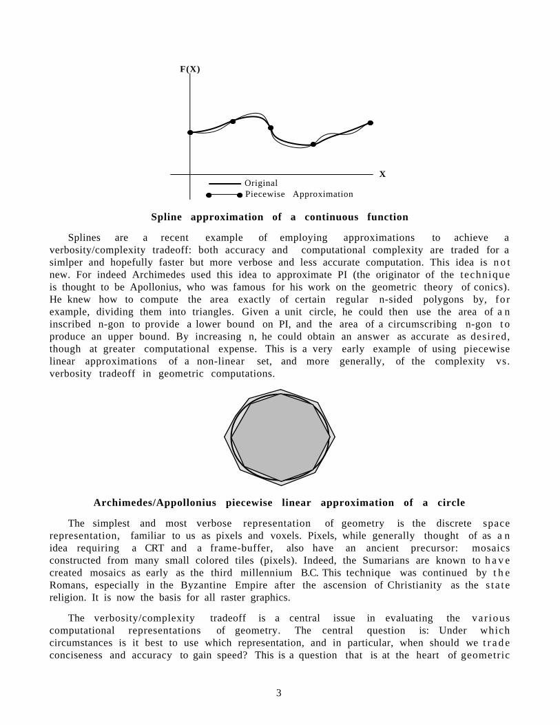
All of this leads us into the realm of approximations, and in particular, to reducing t h ecomputational effort by employing approximations of various forms. During the early y e a r sof Numerical Analysis, it was quickly recognized that finding the roots of polynomials ofmodest degree was not only slow, but was often infeasible due to accumulation of numericalerror. An importance solution to this problem was provided by Splines, a term we now use t odenote the representation of functions (for curves or surfaces) as piecewise polynomials eachof low degree. Any arbitrary function, say one continuous for all derivatives, could b eapproximated arbitrarily well almost everywhere by a set of pieces, each piece being acomputationally appealing function. The only places where unbounded continuity is sacrificedis where the pieces met, called "joins". However, the polynomials can be constrained so t h a tthe resulting approximation will have any desired but bounded degree of continuity at t h ejoins. The resulting spline representation is then much more attractive computationally t h a nthe original complicated function.

3

X

F(X)

OriginalPiecewise Approximation

Spline approximation of a continuous function

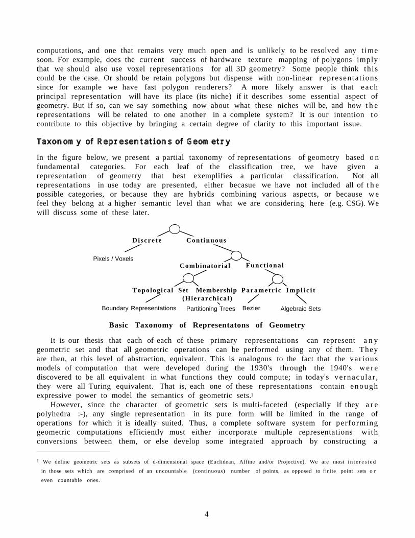
Splines are a recent example of employing approximations to achieve averbosity/complexity tradeoff: both accuracy and computational complexity are traded for asimlper and hopefully faster but more verbose and less accurate computation. This idea is n o tnew. For indeed Archimedes used this idea to approximate PI (the originator of the techniqueis thought to be Apollonius, who was famous for his work on the geometric theory of conics).He knew how to compute the area exactly of certain regular n-sided polygons by, forexample, dividing them into triangles. Given a unit circle, he could then use the area of a ninscribed n-gon to provide a lower bound on PI, and the area of a circumscribing n-gon t oproduce an upper bound. By increasing n, he could obtain an answer as accurate as desired,though at greater computational expense. This is a very early example of using piecewiselinear approximations of a non-linear set, and more generally, of the complexity vs.verbosity tradeoff in geometric computations.

Archimedes/Appollonius piecewise linear approximation of a circle

The simplest and most verbose representation of geometry is the discrete spacerepresentation, familiar to us as pixels and voxels. Pixels, while generally thought of as a nidea requiring a CRT and a frame-buffer, also have an ancient precursor: mosaicsconstructed from many small colored tiles (pixels). Indeed, the Sumarians are known to h a v ecreated mosaics as early as the third millennium B.C. This technique was continued by t h eRomans, especially in the Byzantine Empire after the ascension of Christianity as the s t a t ereligion. It is now the basis for all raster graphics.

The verbosity/complexity tradeoff is a central issue in evaluating the var iouscomputational representations of geometry. The central question is: Under whichcircumstances is it best to use which representation, and in particular, when should we t r a d econciseness and accuracy to gain speed? This is a question that is at the heart of geometric

4

computations, and one that remains very much open and is unlikely to be resolved any t imesoon. For example, does the current success of hardware texture mapping of polygons implythat we should also use voxel representations for all 3D geometry? Some people think th i scould be the case. Or should be retain polygons but dispense with non-linear representa t ionssince for example we have fast polygon renderers? A more likely answer is that eachprincipal representation will have its place (its niche) if it describes some essential aspect ofgeometry. But if so, can we say something now about what these niches will be, and how t h erepresentations will be related to one another in a complete system? It is our intention t ocontribute to this objective by bringing a certain degree of clarity to this important issue.

T a x o n o m y o f R e p r e s e n t a t i o n s o f G e o m e t r y

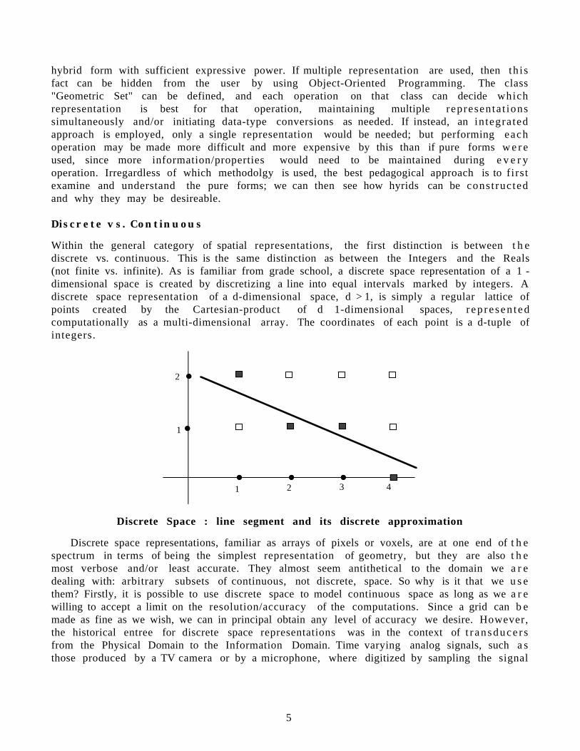
In the figure below, we present a partial taxonomy of representations of geometry based o nfundamental categories. For each leaf of the classification tree, we have given arepresentation of geometry that best exemplifies a particular classification. Not allrepresentations in use today are presented, either becasue we have not included all of t h epossible categories, or because they are hybrids combining various aspects, or because w efeel they belong at a higher semantic level than what we are considering here (e.g. CSG). Wewill discuss some of these later.

Discre t e Cont inuous

Combinatoria l Funct iona l

P a r a m e t r i c I m p l i c i tTopolog ica l Set Membership(Hierarchica l )

Pixels / Voxels

Boundary Representations Partitioning Trees Bezier Algebraic Sets

Basic Taxonomy of Representatons of Geometry

It is our thesis that each of each of these primary representations can represent a n ygeometric set and that all geometric operations can be performed using any of them. Theyare then, at this level of abstraction, equivalent. This is analogous to the fact that the var iousmodels of computation that were developed during the 1930's through the 1940's w e r ediscovered to be all equivalent in what functions they could compute; in today's vernacula r ,they were all Turing equivalent. That is, each one of these representations contain enoughexpressive power to model the semantics of geometric sets.1

However, since the character of geometric sets is multi-faceted (especially if they a r epolyhedra :-), any single representation in its pure form will be limited in the range ofoperations for which it is ideally suited. Thus, a complete software system for performinggeometric computations efficiently must either incorporate multiple representations wi thconversions between them, or else develop some integrated approach by constructing a 1 We define geometric sets as subsets of d-dimensional space (Euclidean, Affine and/or Projective). We are most i n t e r e s t e d

in those sets which are comprised of an uncountable (continuous) number of points, as opposed to finite point sets o r

even countable ones.

5

hybrid form with sufficient expressive power. If multiple representation are used, then th i sfact can be hidden from the user by using Object-Oriented Programming. The class"Geometric Set" can be defined, and each operation on that class can decide whichrepresentation is best for that operation, maintaining multiple representa t ionssimultaneously and/or initiating data-type conversions as needed. If instead, an in tegratedapproach is employed, only a single representation would be needed; but performing eachoperation may be made more difficult and more expensive by this than if pure forms w e r eused, since more information/properties would need to be maintained during e v e r yoperation. Irregardless of which methodolgy is used, the best pedagogical approach is to firstexamine and understand the pure forms; we can then see how hyrids can be const ructedand why they may be desireable.

D i s c r e t e v s . C o n t i n u o u s

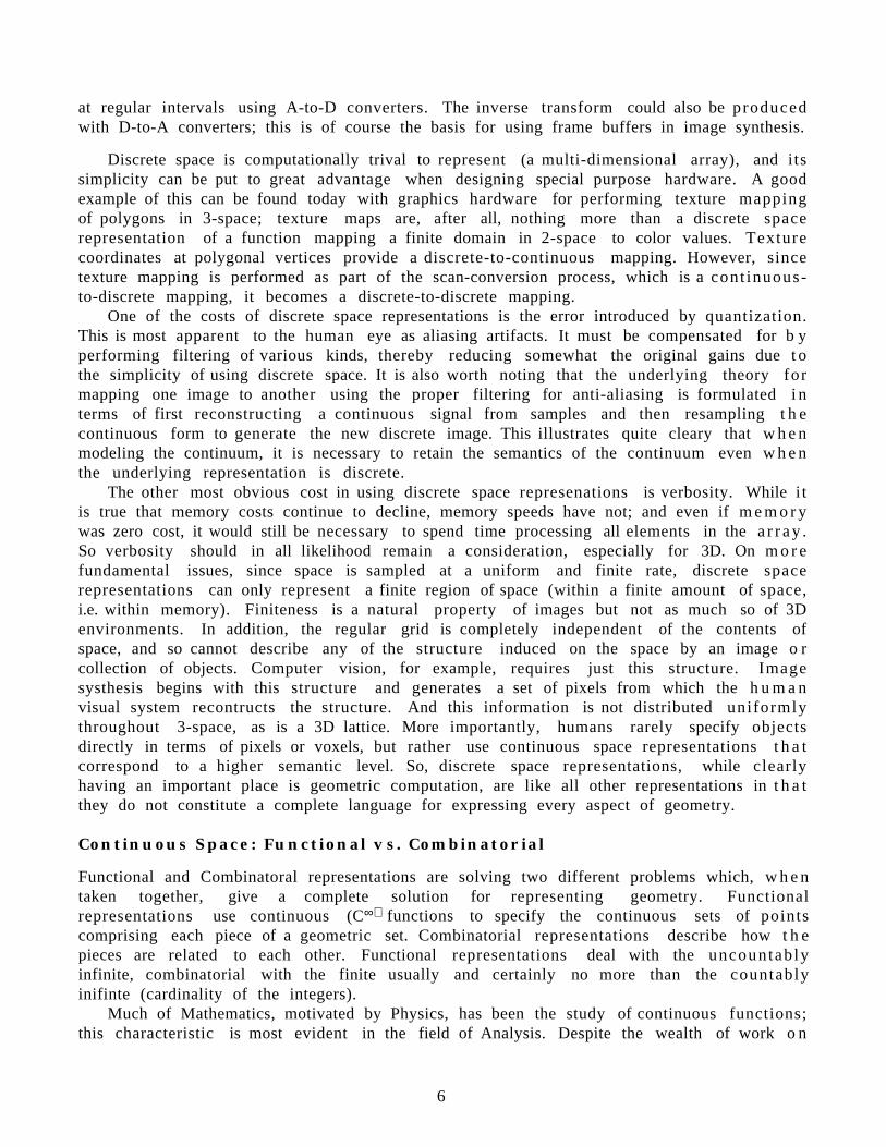
Within the general category of spatial representations, the first distinction is between t h ediscrete vs. continuous. This is the same distinction as between the Integers and the Reals(not finite vs. infinite). As is familiar from grade school, a discrete space representation of a 1 -dimensional space is created by discretizing a line into equal intervals marked by integers. Adiscrete space representation of a d-dimensional space, d > 1, is simply a regular lattice ofpoints created by the Cartesian-product of d 1-dimensional spaces, r ep re sen t edcomputationally as a multi-dimensional array. The coordinates of each point is a d-tuple ofintegers.

1 2 3 4

1

2

Discrete Space : line segment and its discrete approximation

Discrete space representations, familiar as arrays of pixels or voxels, are at one end of t h espectrum in terms of being the simplest representation of geometry, but they are also t h emost verbose and/or least accurate. They almost seem antithetical to the domain we a r edealing with: arbitrary subsets of continuous, not discrete, space. So why is it that we u s ethem? Firstly, it is possible to use discrete space to model continuous space as long as we a r ewilling to accept a limit on the resolution/accuracy of the computations. Since a grid can b emade as fine as we wish, we can in principal obtain any level of accuracy we desire. However,the historical entree for discrete space representations was in the context of t r ansduce r sfrom the Physical Domain to the Information Domain. Time varying analog signals, such a sthose produced by a TV camera or by a microphone, where digitized by sampling the signal

6

at regular intervals using A-to-D converters. The inverse transform could also be producedwith D-to-A converters; this is of course the basis for using frame buffers in image synthesis.

Discrete space is computationally trival to represent (a multi-dimensional array), and itssimplicity can be put to great advantage when designing special purpose hardware. A goodexample of this can be found today with graphics hardware for performing texture mappingof polygons in 3-space; texture maps are, after all, nothing more than a discrete spacerepresentation of a function mapping a finite domain in 2-space to color values. Texturecoordinates at polygonal vertices provide a discrete-to-continuous mapping. However, sincetexture mapping is performed as part of the scan-conversion process, which is a cont inuous-to-discrete mapping, it becomes a discrete-to-discrete mapping.

One of the costs of discrete space representations is the error introduced by quantization.This is most apparent to the human eye as aliasing artifacts. It must be compensated for b yperforming filtering of various kinds, thereby reducing somewhat the original gains due t othe simplicity of using discrete space. It is also worth noting that the underlying theory formapping one image to another using the proper filtering for anti-aliasing is formulated i nterms of first reconstructing a continuous signal from samples and then resampling t h econtinuous form to generate the new discrete image. This illustrates quite cleary that w h e nmodeling the continuum, it is necessary to retain the semantics of the continuum even w h e nthe underlying representation is discrete.

The other most obvious cost in using discrete space represenations is verbosity. While i tis true that memory costs continue to decline, memory speeds have not; and even if m e m o r ywas zero cost, it would still be necessary to spend time processing all elements in the a r r a y .So verbosity should in all likelihood remain a consideration, especially for 3D. On m o r efundamental issues, since space is sampled at a uniform and finite rate, discrete spacerepresentations can only represent a finite region of space (within a finite amount of space,i.e. within memory). Finiteness is a natural property of images but not as much so of 3Denvironments. In addition, the regular grid is completely independent of the contents ofspace, and so cannot describe any of the structure induced on the space by an image o rcollection of objects. Computer vision, for example, requires just this structure. Imagesysthesis begins with this structure and generates a set of pixels from which the h u m a nvisual system recontructs the structure. And this information is not distributed uniformlythroughout 3-space, as is a 3D lattice. More importantly, humans rarely specify objectsdirectly in terms of pixels or voxels, but rather use continuous space representations t h a tcorrespond to a higher semantic level. So, discrete space representations, while clearlyhaving an important place is geometric computation, are like all other representations in t h a tthey do not constitute a complete language for expressing every aspect of geometry.

C o n t i n u o u s S p a c e : F u n c t i o n a l v s . C o m b i n a t o r i a l

Functional and Combinatoral representations are solving two different problems which, w h e ntaken together, give a complete solution for representing geometry. Functionalrepresentations use continuous (C∞) functions to specify the continuous sets of pointscomprising each piece of a geometric set. Combinatorial representations describe how t h epieces are related to each other. Functional representations deal with the uncountablyinfinite, combinatorial with the finite usually and certainly no more than the countablyinifinte (cardinality of the integers).

Much of Mathematics, motivated by Physics, has been the study of continuous functions;this characteristic is most evident in the field of Analysis. Despite the wealth of work o n

7

continuous functions, the problem of having humans design objects has resulted in a nimportant contribution to our understanding of how to represent curves and surfaces usingpolynomials, and how to represent the polynomials themselves. This is most evident in t h edevelopment of the Bezier/Berstein theory and the closely related B-spline theory. Thetraditional "power basis" form describes polynomials in terms of a weighted sum ofmonomials. This turns out to be a direct specification of the behaviour of the polynomialexactly at the origin of the coordinate system in terms of its value and derivatives. The Bezierform instead expresses a polynomial directly as the weighted sum of points (control points)independent of the coordinate system, and its behaviour in the vacintity of these points isunderstandable in terms of these points. So while any polynomial can be expressed in e i t he rthe power or the Berstein basis, the latter has proved to be much more a t t rac t ivecomputationally.

In contrast to Analysis, Computer Science has been principally the study of the finite, albeit in a computational milieu. This is most evident in the use of combinatorial s t ruc tu res ,such as graphs, that provide the basis in computing for data structures. As discussed earlier,a strict devotion to using monolithic but complicated functions for representing objects ismuch less attractive computationally than using many simpler pieces. It is the problem ofrepresenting "the many" that requires the combinatorial component. This can be used t oexpress how the pieces connect to one another or how to organize the pieces hierarchically t osignificantly improve performance. And once we have a combinatorial structure, it is easy t ointroduce the discontinuities absent from the standard representations of continuousfunctions which are C∞. This is most readily perceived if, for example, we interpret a 3Dgeometric model as a function that maps points in 3-space to some set of attributes, such a scolor; surfaces then correspond to discontinuities in this function. Analysis has always h a ddifficulty with discontinuites, often resorting to such devices as representing a sample as t h elimit of an inifinite sequence of continuous functions. This is due to the absence in t h e i rlanguage of adequate means for expressing arbitrary discontinuities. The combinatorialcomponent provides us with just such a language.

F u n c t i o n a l : P a r a m e t r i c s v s . I m p l i c i t s

An important distinction for the functional form is between parametrics and implicits. This isnothing more than the difference between whether the set lies in the range or the domain ofa function, respectively. The computational impact of this distinction manifest in var iousgeometric operations. Parametrics are naturally suited for generating a finite sampling ofpoints while implicits facilitate computing intersections.

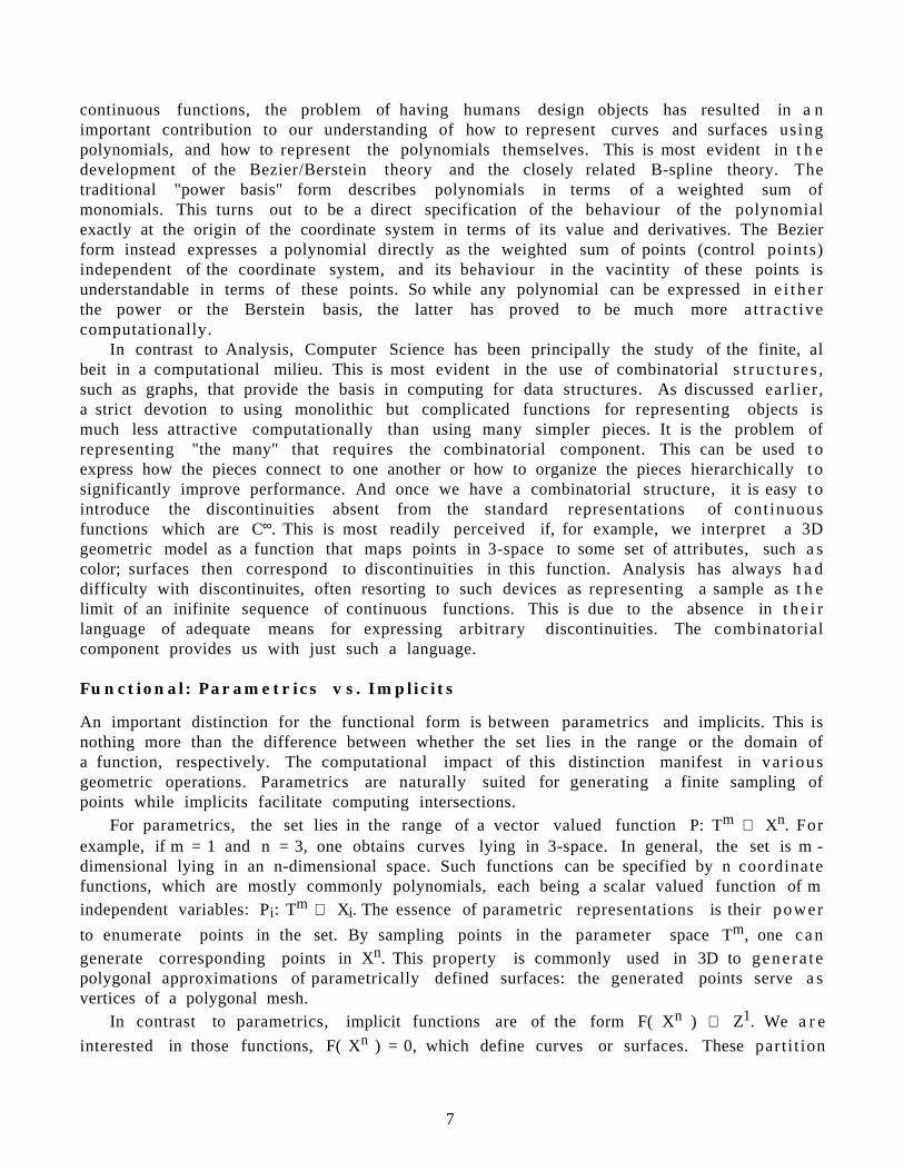
For parametrics, the set lies in the range of a vector valued function P: Tm ⇒ Xn. Forexample, if m = 1 and n = 3, one obtains curves lying in 3-space. In general, the set is m -dimensional lying in an n-dimensional space. Such functions can be specified by n coordinatefunctions, which are mostly commonly polynomials, each being a scalar valued function of mindependent variables: Pi: Tm ⇒ Xi. The essence of parametric representations is their power

to enumerate points in the set. By sampling points in the parameter space Tm, one c a ngenerate corresponding points in Xn. This property is commonly used in 3D to genera tepolygonal approximations of parametrically defined surfaces: the generated points serve a svertices of a polygonal mesh.

In contrast to parametrics, implicit functions are of the form F( Xn ) ⇒ Z1. We a r e

interested in those functions, F( Xn ) = 0, which define curves or surfaces. These part i t ion

8

space into a collection of connected regions such that each region is entirely in F( Xn) > 0 or F(Xn) < 0. We can then use these to define solids in 3D as those points that satisfy F( Xn) <= 0 ( o rF( Xn) >= 0). This gives us a membership function (also called a characteristic function) for t h eset. A membership function allows us to determine for any point in space whether it is amember of the set by evaluating the function. This is the essential computationalcharacteristic of implicit representations.

Currently, the most popular forms of parametric and implicit functions use polynomials(with rational coefficients). Sets defined in the implicit form by a single polynomial define t h eclass called Algebraic Sets. Surfaces defined parameterically by (rational) polynomialcoordinate functions are also algebraic sets; but not all algebraic sets admit such aparameterization. Thus, parametrics are a subset of the implicits when only polynomials a r einvolved. Determining the implicit form of a parametric surface is called implicitization, whiledetermining a parametric form of an implicit is called parameterization. However, neither ofthese is easy to do in general, requiring techniques from Algebraic Geometry. The o n enotable exception is when only quadratic polynomials are used, in which case both forms a r ewell known; and quadratic rational parametrics and quadratic implicits define exactly t h esame class of sets.

The distinction between sets for which one has a membership function, as with implicits,and those for which one has an enumeration function, as with parametrics, lies at the v e r yfoundations of the theory of computation. In order for a (countable) set to be characterized a scomputable, the set must have a computable membership function. Such sets are calledRecursive Sets. Those sets for which there exist computable enumera t ing /genera t ingfunctions are called Recursively Enumerable Sets. For any recursive set, there exists, i naddition to its membership function, a computable generating function for the set, and so t h eRecursive Sets are also Recursively Enumerable. However, the reverse is not the case, and sothe Recursive Sets are a proper subset of the Recursively Enumerable Sets, the later beingcalled semi-computable. This strongly suggests that the distinction between implicits a n dparametrics corresponds to an important difference in methods of defining sets. (The fact t h a tpolynomially define parametrics are a subset of the implicits, rather than the reverse a ssuggested by recursive sets being a subset of the recursively enumerable, may be an artifactof considering only polynomials.)

The difference in the computational efficacy of the two representations can be largelyunderstood in terms of the difference between membership and enumeration functions.Determining set membership is required for performing any intersection operation ( t h epoints of intersection are those which are members of both sets). Such geometric operationsinclude point classification, ray-surface intersection, clipping to a view-volume, collisiondetection, constructive solid geometry, radiosity, shadows, etc. On the other hand ,enumeration is used directly for polygonalization of a curved surface and scan-conversion ofpolygons. However, the parametric form can be use to compute intersections qui teeffectively if paired with an implicit. This is commonly done when a parametr icrepresentation of a line (ray or edge) is substituted into an implicit equation of a surface.Various values of the parameter are "enumerated" either analytically if the degree is 1 or 2 ,or numerically by a iterative technique such as Newton iteration.

C o m b i n a t o r i a l : T o p o l o g i c a l v s . S e t M e m b e r s h i p

9

Given an object defined by a collection of functionally defined continuous pieces, we m u s torganize them into a whole using combinatorial structures. Currently, combinatorialstructures, i.e. graphs, have been used primary to express two fundamental relationsbetween components of a set: the topological structure and the set membership structure.

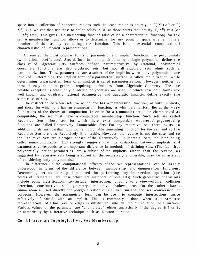
The topological structure encodes the incidence relations between geometric elements, i.e.which elements "touch" which other elements. These elements may be of the same dimension,such as polyhedral faces which share an edge, or they may be of differing dimensions, a sbetween a polygon and the edges that bound it. This structure is represented by a g r a p hwhere each node corresponds to an element and graph edges correspond to the incidencerelation. It also has a hierarchical structure in which levels of the hierarchy correspond t othe various dimensions of the components. Other topological properties, such as number ofconnected components and genus of each components, can be computed from this graph. Thetopological form is the basis for the many varieties of boundary representations. As aconsequence, for 3D it is most closely associated with surface representations, a l thoughvolumes be easily included in the schema by adding the appropriate nodes for each 3 -dimensional connected region of space (such as F1in the figure below).

V 1

V 2 V 3

V 4

V 5 V 6

E1

E2

E3

E4

E5

E6

2 D - s e t

M1

E1 E2 E3

V 1 V 2 V 3

1 D - s e t

0 D - s e t

F 1

1D-man i fo ld

0D-man i fo ld

M2

E4 E5 E6

V 4 V 5 V 6

Topological Representation

Representing set membership is more closely identified with volumetric representa t ionsthan with boundary representations, and the collection of elements are usually not the s a m eas those defined by using the topological properties. Most commonly, the elements are regionsof space created as a consequence of forming a hierarchical search structure whose purposeis to accelerate intersection and/or visibility calculations. These include octrees, boundingvolume hierarchies, and binary space partitioning trees. They all accelerate intersectionsusing the same prinicpal: the bounding volume principal. If some geometry entity, such as apoint, ray or object, does not intersect a region/bounding-volume, then the entity cannotintersect any contents of that region: (B subset of A) & not (C subset of A) ⇒ not (B ∩ C). Thusthe set membership relation confers transitively the non-intersection property. Similarly, ifa region has visibility priority over another region, then the set membership relation confersvisibility priority transitively.

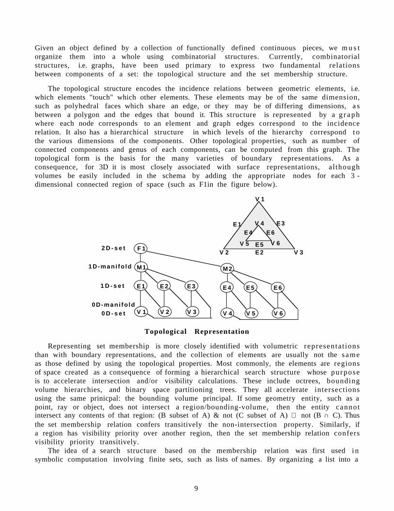
The idea of a search structure based on the membership relation was first used i nsymbolic computation involving finite sets, such as lists of names. By organizing a list into a

1 0

binary search tree, various operations, such as "find", "insert" and "delete", could b eperformed in O( log n) rather than O( n ) time, and even better when the statisticaldistribution of the input was known to be other than uniform.

0 1 2 3 4 5 6 7 8

5

0 8

64

1

<0

0 - 1 1 - 4

4 - 5 5 - 6 6 - 8

>8

x < 5 x > 5

x < 8x > 0

Binary Search Tree for the set 0,1,4,5,6,8

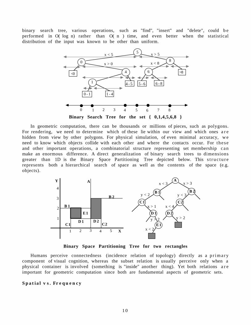
In geometric computation, there can be thousands or millions of pieces, such as polygons.For rendering, we need to determine which of these lie within our view and which ones a r ehidden from view by other polygons. For physical simulation, of even minimal accuracy, w eneed to know which objects collide with each other and where the contacts occur. For t h e s eand other important operations, a combinatorial structure representing set membership c a nmake an enormous difference. A direct generalization of binary search trees to dimensionsgreater than 1D is the Binary Space Partitioning Tree depicted below. This s t r u c t u r erepresents both a hierarchical search of space as well as the contents of the space (e.g.objects).

X

Y

31 2 4 5

1

2

3

4

A

B 2

B 1

C1 C2D 1 D 2

E 1

Ax < 3 x > 3

B 1 B 2

C2C1

D 1 D 2

y < 2 y < 3

x < 4x > 1

E 1y > 2

x < 2

y > 2

Binary Space Partitioning Tree for two rectangles

Humans perceive connectedness (incidence relation of topology) directly as a p r i m a r ycomponent of visual cognition, whereas the subset relation is usually perceive only when aphysical container is involved (something is "inside" another thing). Yet both relations a r eimportant for geometric computation since both are fundamental aspects of geometric sets.

S p a t i a l v s . F r e q u e n c y

1 1

It is somewhat counter-intuitive that "geometry", which is almost synonymous with the term"spatial", can be represented in a non-spatial way, in particular, represented in t h efrequency domain, as is natural to do for something like sound waves. For indeed mos tgeometric features are non-periodic and local, while sine waves are exactly the opposite,periodic and global (from -inf to +inf). For representing geometry, this incompatibility h a srequired introducing locality into the frequency paradigm to produce something of a h y b r i dfrequency/spatial schema. Initially, this was accomplished by such mechanisms as t h e"Windowed Fourier Transform".

But more recently, this difficulty has been addresses by the use of "wavelets". Thistechnique replaces sine and cosine, which are the Fourier Transform basis functions and a r enon-zero over an infinite domain (possessing "infinite support"), with ones that are non-ze roover only a finite domain (possessing local support), such as an isolated square pulse.However, local support has a price in the frequency domain: the Fourier Transform of such afunction has infinite support in Fourier-space, another form of the uncertainity principle. Awavelet transform begins with a single generating (mother) wavelet, and then it is scaled,often by 2-n, n > 0, and translated to create a collection of basis functions. In the typical case,this scaling and translating of a function with local support results in a hierarchical spatialsubdivision analogous to a quadtree (in 2D). Thus, achieving a truely effective use of t h efrequency concept for representing geometry has led to the introduction of an increasinglygeometric character. Given the success of frequency domain based operations forimage/video compression and the emerging wavelet theory, we would expect s u c hfrequency/spatial hybrid schemes to become much more widely used for geometriccomputation in the future.

Voxels as a Computational Representation of Geometry

Arie E. Kaufman

Computer Science DepartmentState University of New York at Stony Brook

Stony Brook, NY 11794-4400ari@cs.sunysb.edu

http://www.cs.sunysb.edu

Abstract

This paper is a survey of volume visualization, volume graphics, and volume rendering techniques. Itfocuses specifically on the use of the voxel representation and volumetric techniques for geometricapplications.

1. Introduction

Volume data are 3D entities that may have information inside them, might not consist of surfaces andedges, or might be too voluminous to be represented geometrically .Volume visualizationis a methodof extracting meaningful information from volumetric data using interactive graphics and imaging, andit is concerned with volume data representation, modeling, manipulation, and rendering [49]. Volumedata are obtained by sampling, simulation, or modeling techniques. For example, a sequence of 2Dslices obtained from Magnetic Resonance Imaging (MRI) or Computed Tomography (CT) is 3Dreconstructed into a volume model and visualized for diagnostic purposes or for planning of treatmentor surgery. The same technology is often used with industrial CT for non-destructive inspection ofcomposite materials or mechanical parts. Similarly, confocal microscopes produce data which isvisualized to study the morphology of biological structures. In many computational fields, such as incomputational fluid dynamics, the results of simulation typically running on a supercomputer are oftenvisualized as volume data for analysis and verification. Recently, many traditional geometric computergraphics applications, such as CAD and simulation, have been exploiting the advantages of volumetechniques calledvolume graphicsfor modeling, manipulation, and visualization.

Over the years many techniques have been developed to visualize 3D data. Since methods fordisplaying geometric primitives were already well-established, most of the early methods involveapproximating a surface contained within the data using geometric primitives. When volumetric dataare visualized using a surface rendering technique, a dimension of information is essentially lost. Inresponse to this, volume rendering techniques were developed that attempt to capture the entire 3D datain a single 2D image. Volume rendering convey more information than surface rendering images, but atthe cost of increased algorithm complexity, and consequently increased rendering times. To improveinteractivity in volume rendering, many optimization methods as well as several special-purpose volumerendering machines have been developed.

We begin with an introduction to volumetric data. Section 3 covers briefly surface rendering techniquesfor volume data. Section 4 discusses in details volume rendering techniques, including image-order,object-order, and domain techniques. Optimization methods for volume rendering are discussed inSection 5, and special-purpose volume rendering hardware is described in Section 6. Section 7introduces global illumination of volumetric data, including volumetric ray tracing and volumetricradiosity. Irregular grid rendering is briefly discussed in Section 8. Volume graphics is introduced in

-2-

Section 9, including several volume modeling techniques, such as voxelization, texture mapping,amorphous phenomena, block operations, constructive solid modeling, and volume sculpting.

2. Volumetric Data

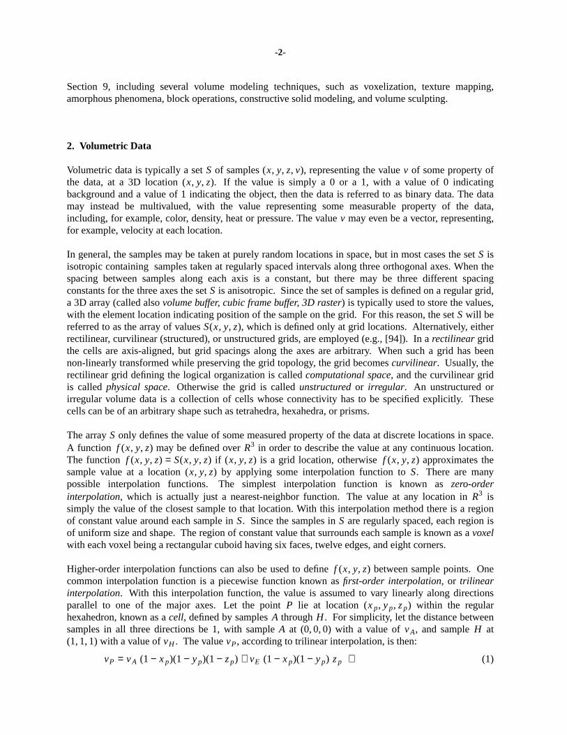
Volumetric data is typically a setS of samples (x, y, z, v), representing the valuev of some property ofthe data, at a 3D location (x, y, z). If the value is simply a 0 or a 1, with a value of 0 indicatingbackground and a value of 1 indicating the object, then the data is referred to as binary data. The datamay instead be multivalued, with the value representing some measurable property of the data,including, for example, color, density, heat or pressure. The valuev may even be a vector, representing,for example, velocity at each location.

In general, the samples may be taken at purely random locations in space, but in most cases the setS isisotropic containing samples taken at regularly spaced intervals along three orthogonal axes. When thespacing between samples along each axis is a constant, but there may be three different spacingconstants for the three axes the setS is anisotropic. Since the set of samples is defined on a regular grid,a 3D array (called alsovolume buffer, cubic frame buffer, 3D raster) is typically used to store the values,with the element location indicating position of the sample on the grid. For this reason, the setS will bereferred to as the array of valuesS(x, y, z), which is defined only at grid locations. Alternatively, eitherrectilinear, curvilinear (structured), or unstructured grids, are employed (e.g., [94]). In arectilinear gridthe cells are axis-aligned, but grid spacings along the axes are arbitrary. When such a grid has beennon-linearly transformed while preserving the grid topology, the grid becomescurvilinear. Usually, therectilinear grid defining the logical organization is calledcomputational space,and the curvilinear gridis calledphysical space. Otherwise the grid is calledunstructuredor irregular. An unstructured orirregular volume data is a collection of cells whose connectivity has to be specified explicitly. Thesecells can be of an arbitrary shape such as tetrahedra, hexahedra, or prisms.

The arrayS only defines the value of some measured property of the data at discrete locations in space.A function f (x, y, z) may be defined overR3 in order to describe the value at any continuous location.The function f (x, y, z) = S(x, y, z) if ( x, y, z) is a grid location, otherwisef (x, y, z) approximates thesample value at a location (x, y, z) by applying some interpolation function toS. There are manypossible interpolation functions. The simplest interpolation function is known aszero-orderinterpolation, which is actually just a nearest-neighbor function. The value at any location inR3 issimply the value of the closest sample to that location. With this interpolation method there is a regionof constant value around each sample inS. Since the samples inS are regularly spaced, each region isof uniform size and shape. The region of constant value that surrounds each sample is known as avoxelwith each voxel being a rectangular cuboid having six faces, twelve edges, and eight corners.

Higher-order interpolation functions can also be used to definef (x, y, z) between sample points. Onecommon interpolation function is a piecewise function known asfirst-order interpolation, or trilinearinterpolation. With this interpolation function, the value is assumed to vary linearly along directionsparallel to one of the major axes. Let the pointP lie at location (xp, yp, zp) within the regularhexahedron, known as acell, defined by samplesA throughH . For simplicity, let the distance betweensamples in all three directions be 1, with sampleA at (0, 0, 0) with a value ofvA, and sampleH at(1, 1, 1) with a value ofvH . The valuevP, according to trilinear interpolation, is then:

(1)vP = vA (1 − xp)(1 − yp)(1 − zp) + vE (1 − xp)(1 − yp) zp +

-3-

vB xp (1 − yp)(1 − zp) + vF xp (1 − yp) zp +

vC (1 − xp) yp (1 − zp) + vG (1 − xp) yp zp +

vD xp yp (1 − zp) + vH xp yp zp

In general,A will be at some location (xA, yA, zA), andH will be at (xH ,yH ,zH ). In this case,xp in

Equation 1 would be replaced by(xp − xA)

(xH − xA), with similar substitutions made foryp andzp.

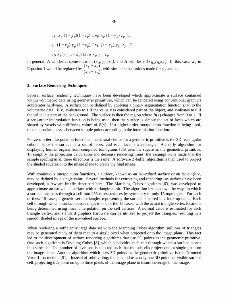
3. Surface Rendering Techniques

Several surface rendering techniques have been developed which approximate a surface containedwithin volumetric data using geometric primitives, which can be rendered using conventional graphicsaccelerator hardware. A surface can be defined by applying a binary segmentation functionB(v) to thevolumetric data.B(v) evaluates to 1 if the valuev is considered part of the object, and evaluates to 0 ifthe valuev is part of the background. The surface is then the region whereB(v) changes from 0 to 1. Ifa zero-order interpolation function is being used, then the surface is simply the set of faces which areshared by voxels with differing values ofB(v). If a higher-order interpolation function is being used,then the surface passes between sample points according to the interpolation function.

For zero-order interpolation functions, the natural choice for a geometric primitive is the 3D rectangularcuboid, since the surface is a set of faces, and each face is a rectangle. An early algorithm fordisplaying human organs from computed tomograms [35] uses the square as the geometric primitive.To simplify the projection calculation and decrease rendering times, the assumption is made that thesample spacing in all three directions is the same. A software Z-buffer algorithm is then used to projectthe shaded squares onto the image plane to create the final image.

With continuous interpolation functions, a surface, known as aniso-valued surfaceor an iso-surface,may be defined by a single value. Several methods for extracting and rendering iso-surfaces have beendeveloped, a few are briefly described here. The Marching Cubes algorithm [63] was developed toapproximate an iso-valued surface with a triangle mesh. The algorithm breaks down the ways in whicha surface can pass through a cell into 256 cases, reduces by symmetry to only 15 topologies. For eachof these 15 cases, a generic set of triangles representing the surface is stored in a look-up table. Eachcell through which a surface passes maps to one of the 15 cases, with the actual triangle vertex locationsbeing determined using linear interpolation on the cell vertices. A normal value is estimated for eachtriangle vertex, and standard graphics hardware can be utilized to project the triangles, resulting in asmooth shaded image of the iso-valued surface.

When rendering a sufficiently large data set with the Marching Cubes algorithm, millions of trianglesmay be generated many of them map to a single pixel when projected onto the image plane. This factled to the development of surface rendering algorithms that use 3D points as the geometric primitive.One such algorithm is Dividing Cubes [8], which subdivides each cell through which a surface passesinto subcells. The number of divisions is selected such that the subcells project onto a single pixel onthe image plane. Another algorithm which uses 3D points as the geometric primitive is the TrimmedVoxel Lists method [91]. Instead of subdividing, this method uses only one 3D point per visible surfacecell, projecting that point on up to three pixels of the image plane to insure coverage in the image.

-4-

4. Volume Rendering Techniques

Representing a surface contained within a volumetric data set using geometric primitives can be usefulin many applications, however there are several main drawbacks to this approach. First, geometricprimitives can only approximate surfaces contained within the original data. Adequate approximationsmay require an excessive amount of geometric primitives. Therefore, a trade-off must be made betweenaccuracy and space requirements. Second, since only a surface representation is used, much of theinformation contained within the data is lost during the rendering process. For example, in CT scanneddata useful information is contained not only on the surfaces, but within the data as well. Also,amorphous phenomena, such as clouds, fog, and fire cannot be adequately represented using surfaces,and therefore must have a volumetric representation, and must be displayed using volume renderingtechniques.

In the next subsections various volume rendering techniques are explored.Volume renderingis theprocess of creating a 2D image directly from 3D volumetric data. Although several of the methodsdescribed in these subsections render surfaces contained within volumetric data, these methods operateon the actual data samples, without the intermediate geometric primitive representations used by thealgorithms in Section 3.

Volume rendering can be achieved using anobject-order, an image-order, or adomain-basedtechnique.Object-order volume rendering techniques use aforward mappingscheme where the volume data ismapped onto the image plane. In image-order algorithms, abackward mappingscheme is used whererays are cast from each pixel in the image plane through the volume data to determine the final pixelvalue. In a domain-based technique the spatial volume data is first transformed into an alternativedomain, such as compression frequency, and wav elet, and then a projection is generated directly fromthat domain.

4.1. Object-Order Techniques

Object-order techniques involve mapping the data samples on to the image plane. One way toaccomplish a projection of a surface contained within the volume is to loop through the data samples,projecting each sample which is part of the object onto the image plane. For this algorithm, the datasamples are binary voxels, with a value of 0 indicating background and a value of 1 indicating theobject. Also, the data samples are on a grid with uniform spacing in all three directions.

If an image is produced by projecting all voxels with a value of 1 to the image plane in an arbitraryorder, we are not guaranteed a correct image. If two voxels project to the same pixel on the image plane,the one that was projected later will prevail, even if it is farther from the image plane than the earlierprojected voxel. This problem can be solved by traversing the data samples in aback-to-frontorder.For this algorithm, the strict definition of back-to-front can be relaxed to require that if two voxelsproject to the same pixel on the image plane, the first processed voxel must be farther away from theimage plane than the second one. This can be accomplished by traversing the data plane-by-plane, androw-by-row inside each plane. For arbitrary orientations of the data in relation to the image plane, someaxes may be traversed in an increasing order, while others may be considered in a decreasing order. Thetraversal can be accomplished with three nested loops, indexing onx, y, andz. Although the relativeorientations of the data and the image plane specify whether each axis should be traversed in anincreasing or decreasing manner, the ordering of the axes in the traversal is arbitrary.

-5-

An alternative to back-to-front projection is afront-to-backmethod in which the voxels are traversed inthe order of increasing distance from the image plane. Although a back-to-front method is easier toimplement, a front-to-back method has the advantage that once a voxel is projected onto a pixel, othervoxels which project to the same pixel are ignored, since they would be hidden by the first voxel.Another advantage of front-to-back projection methods is that if the axis which is most parallel to theviewing direction is chosen to be the outermost loop of the data traversal, meaningful partial imageresults can be displayed to the user. This allows the user to better interact with the data and terminatethe image generation if, for example, an incorrect view direction was selected. Partial image results canbe displayed to the user during a back-to-front method also, but the value of a pixel may change manytimes during image generation. With a front-to-back method, once a pixel value is set, its value remainsunchanged.

Clipping planes orthogonal to the three major axes, and clipping planes parallel to the view plane areeasy to implement using either a back-to-front or a front-to-back algorithm. For orthogonal clippingplanes, the traversal of the data is limited to a smaller rectangular region within the full data set. Toimplement clipping planes parallel to the image plane, data samples whose distance to the image planeis less than the distance between the cut plane and the image plane are ignored. This ability to explorethe whole data set is a major difference between volume rendering techniques and the surface renderingtechniques described in Section 3. In surface rendering techniques, the geometric primitiverepresentation of the object need to be changed in order to implement cut planes, which could be a time-consuming process. In a back-to-front method, cut planes can be achieved by simply modifying thebounds of the data traversal, and utilizing a condition when placing depth values in the image planepixels.

For each voxel, its distance to the image plane could be stored in the pixel to which it maps along withthe voxel value. At the end of a data traversal a 2D array of depth values, called a Z-buffer, is created,where the value. at each pixel in the Z-buffer is the distance to the closest non-empty voxel. A 2Ddiscrete shading technique can then be applied to the image, resulting in a shaded image suitable fordisplay. The 2D discrete shading techniques described here take as input a 2D array of depth values anda 2D array of projected voxel values, and produce as output a 2D image of intensity values. Thesimplest 2D discrete shading method is known as depth shading, ordepth-only shading[36, 103], whereonly the Z-buffer is used and the intensity value stored in each pixel of the output image is inverselyproportional to the depth of the corresponding input pixel. This produces images where features farfrom the image plane appear dark, while close feature are bright. Since surface orientation is notconsidered in this shading method, most details such as surface discontinuities and object boundaries arelost.

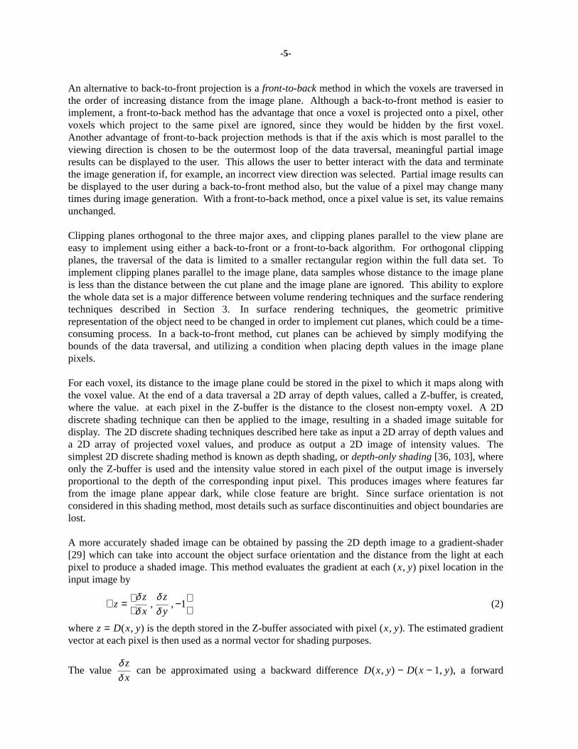
A more accurately shaded image can be obtained by passing the 2D depth image to a gradient-shader[29] which can take into account the object surface orientation and the distance from the light at eachpixel to produce a shaded image. This method evaluates the gradient at each (x, y) pixel location in theinput image by

(2)∇z =

δ z

δ x,

δ z

δ y, −1

wherez = D(x, y) is the depth stored in the Z-buffer associated with pixel (x, y). The estimated gradientvector at each pixel is then used as a normal vector for shading purposes.

The valueδ z

δ xcan be approximated using a backward differenceD(x, y) − D(x − 1, y), a forward

-6-

difference D(x + 1, y) − D(x, y), or a central difference1

2(D(x + 1, y) − D(x − 1, y)). Similar

equations are used for approximatingδ z

δ y. In general, the central difference is a better approximation of

the derivative, but along object edges where, for example, pixels (x, y) and (x + 1, y) belong to twodifferent objects, a backward difference would provide a better approximation. A context sensitivenormal estimation method [120] was developed to provide more accurate normal estimations bydetecting image discontinuities. In this method, two pixels are considered to be in the same ‘‘context’’if their depth values, and the first derivative of the depth at these locations do not greatly differ. Thegradient vector at some pixelp is then estimated by considering only those pixels which lie within auser-defined neighborhood, and belong to the same context asp. This ensures that sharp object edges,and slope changes are not smoothed out in the final image.

The previous rendering methods consider only binary data samples where a value of 1 indicates theobject and a value of 0 indicates the background. Many forms of data acquisition (e.g., CT) producedata samples with 8, 12, or even more bits of data per sample. If these data samples represent the valuesat some sample points, and the value vary according to some convolution applied to the data sampleswhich can reconstruct the original 3D signal, then a scalar field which approximates the original 3Dsignal has been defined.

One way to reconstruct the original signal is, as described previously, to define a functionf (x, y, z)which determines the value at any location in space. This technique is typically employed by backward-mapping (image-order) algorithms. In forward mapping algorithms, the original signal is reconstructedby spreading the value at a data sample into space. Westover describes a splatting algorithm [111] forapproximating smooth object-ordered volume rendering, in which the value of the data samplesrepresents a density. Each data samples = (xs,ys,zs,ρ(s)), s∈S, has a functionC defining itscontribution to every point (x, y, z) in the space:

(3)Cs(x, y, z) = hv(x − xs, y − ys, z − zs)ρ(s)

wherehv is the volume reconstruction kernel andρ(s) is the density of samples which is located at(xs, ys, zs). The contribution of a samples to an image plane pixel (x, y) can then be computed byintegration:

(4)Cs(x, y) = ρ(s)∞

−∞∫ hv(x − xs, y − ys, u)du

where theu coordinate axis is parallel to the view ray. Since this integral is independent of the sampledensity, and depends only on its (x, y) projected location, a footprint functionF can be defined asfollows:

(5)F(x, y) =∞

−∞∫ hv(x, y, u)du

where (x, y) is the displacement of an image sample from the center of the sample’s image planeprojection. The weightw at each pixel can then be expressed as:

(6)w (x, y)s = F(x − xs, y − ys)

where (x, y) is the pixel location, and (xs, ys) is the image plane location of the samples.

A footprint table can be generated by evaluating the integral in Equation 5 on a grid with a resolutionmuch higher than the image plane resolution. All table values lying outside of the footprint table extent

-7-

have zero weight and therefore need not be considered when generating an image. A footprint table fora data samples, can be centered on the projected image plane location ofs, and be sampled in order todetermine the weight of the contribution ofs to each pixel on the image plane. Multiplying this weightby ρ(s) then gives the contribution ofs to each pixel.

Computing a footprint table can be difficult due to the integration required. Discrete integrationmethods can be used to approximate the continuous integral, but generating a footprint table is still acostly operation. Luckily, for orthographic projections, the footprint of each sample is the same exceptfor an image plane offset. Therefore, only one footprint table needs to be calculated per view. Since thisstill would require too much computation time, only one generic footprint table is built for the kernel.For each view, a view-transformed footprint table is created from the generic footprint table. Thegeneric footprint table can be precomputed, therefore, it does not matter how long the computationtakes.

Generating a view-transformed footprint table from the generic footprint table can be accomplished inthree steps. First, the image plane extent of the projection of the reconstruction kernel is determined.Next a mapping is computed between this extent and the extent that surrounds the generic footprinttable. Finally, the value for each entry in the view-transformed footprint table is determined by mappingthe location of the entry to the generic footprint table, and sampling. The extent of the reconstructionkernel is either a sphere, or is bounded by a sphere, so the extent of the generic footprint table is alwaysa circle. If the grid spacing of the data samples is uniform along all three axes, then the reconstructionkernel is a sphere and the image plane extent of the reconstruction kernel will be a circle. The mappingfrom this extent to the extent of the generic footprint table is simply a scaling operation. If the gridspacing differs along the three axes, then the reconstruction kernel is an ellipsoid and the image planeextent of the reconstruction kernel will be an ellipse. In this case, a mapping from this ellipse to thecircular extent of the generic footprint table must be computed.

There are three modifiable parameters in this algorithm which can greatly affect image quality. First,the size of the footprint table can be varied. Small footprint tables produce blocky images, while largefootprint tables may smooth out details and require more space. Second, different sampling methodscan be used when generating the view-transformed footprint table from the generic footprint table.Using a nearest-neighbor approach is fast, but may produce aliasing artifacts. On the other hand, usingbilinear interpolation produces smoother images at the expense of longer rendering times. The thirdparameter which can be modified is the reconstruction kernel itself. The choice of, for example, a conefunction, Gaussian function, sync function or bilinear function affects the final image.

Drebin, Carpenter, and Hanrahan [16] developed a technique for rendering volumes that containmixtures of materials, such as CT data containing bone, muscle and flesh. In this method, variousassumptions about the volume data are made. First, it is assumed that the scalar field was sampledabove the Nyquist frequency, or a low-pass filter was used to remove high frequencies before sampling.The volume contains either several scalar fields, or one scalar field representing the composition ofseveral materials. If the latter is the case, it is assumed that material can be differentiated either by thescalar value at each point, or by additional information about the composition of each volume element.

The first step in this rendering algorithm is to create new scalar fields from the input data, known asmaterial percentage volumes. Each material percentage volume is a scalar field representing only onematerial. Color and opacity are then associated with each material, with composite color and opacityobtained by linearly combining the color and opacity for each material percentage volume. A mattevolume, that is, a scalar field on the volume with values ranging between 0 and 1, is used to slice the

-8-

volume or perform other spatial set operations. Actual rendering of the final composite scalar field isobtained by transforming the volume so that one axis is perpendicular to the image plane. The data isthen projected plane by plane in a back-to-front manner and composited to form the final image.

4.2. Image-Order Techniques

Image-order volume rendering techniques are fundamentally different from object-order renderingtechniques. Instead of determining how a data sample affects the pixels on the image plane, in animage-order technique we determine for each pixel on the image plane, the data samples contribute to itare determined.

One of the first image-order volume rendering techniques, which may be calledbinary ray casting[101], was developed to generate images of surfaces contained within binary volumetric data withoutthe need to explicitly perform boundary detection and hidden-surface removal. For each pixel on theimage plane, a ray is cast from that pixel to determine if it intersects the surface contained within thedata. For parallel projections, all rays are parallel to the view direction, where as for perspectiveprojections, rays are cast from the eye point according to the view direction and the field of view. If anintersection does occur, shading is performed at the intersection point, and the resulting color is placedin the pixel. In order to determine the first intersection along the ray a stepping technique is used wherethe value is determined at regular intervals along the ray until the object is intersected. Data sampleswith a value of 0 are considered to be the background while those with a value of 1 are considered to bepart of the object. A zero-order interpolation technique is used, so the value at a location along the rayis 0 if that location is not in any voxel of the data, otherwise it is the value of the closest data sample.For a step sized, thei th point samplepi would be taken at a distancei×d along the ray. For a given ray,either all point samples along the ray have a value of 0 (the ray missed the object entirely), or there issome samplepi taken at a distancei×d along the ray, such that all samplespj , j < i , hav e a value of 0,and samplepi has a value of 1. Point samplepi is then considered to be the first intersection along theray. In this algorithm, the step sized must be chosen carefully. Ifd is too large, small features in thedata may not be detected. On the other hand, ifd is small, the intersection point is more accuratelyestimated at the cost of higher computation time.

There are several optimizations which can be made to this algorithms. First, the number of steps whichmust be made along each ray can be reduced by traversing only the part of the ray contained within thebounding box of the data. A second optimization involves the representation of the data in memory.This algorithm was originally developed on a machine with only 32K of RAM, so data compression wasa critical issue. Instead of simply storing the data as a binary array of 0’s and 1’s, a scan-linerepresentation can be used. For each scan-line in the data, a list of end points can be stored whichrepresent the segments belonging to the object. This representation is compact, yet does not add toomuch time to the intersection calculation.

The previous algorithm deals with the display of surfaces within binary data. A more general algorithmcan be used to generate surface and composite projections of multivalued data. Instead of traversing acontinuous ray and determining the closest data sample for each step with a zero-order interpolationfunction, a discrete representation of the ray could be traversed. This discrete ray is generated using a3D Bresenham-like algorithm or a 3D line scan-conversion (voxelization) algorithm [43, 49] (seeSection 9.1). As in the previous algorithms, for each pixel in the image plane, the data samplescontribute to it need to be determined. This could be done by casting a ray from each pixel in thedirection of the viewing ray. This ray would be discretized (voxelized), and the contribution from each

-9-

voxel along the path is considered when producing the final pixel value. This technique is referred to asdiscrete ray casting[122].

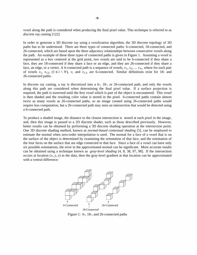
In order to generate a 3D discrete ray using a voxelization algorithm, the 3D discrete topology of 3Dpaths has to be understood. There are three types of connected paths: 6-connected, 18-connected, and26-connected, which are based upon the three adjacency relationships between consecutive voxels alongthe path. An example of these three types of connected paths is given in Figure 1. Assuming a voxel isrepresented as a box centered at the grid point, two voxels are said to be 6-connected if they share aface, they are 18-connected if they share a face or an edge, and they are 26-connected if they share aface, an edge, or a vertex. A 6-connected path is a sequence of voxels,v1, v2, ... vN , where for each pairof voxels vi , vi+1 (1 ≤ i < N), vi and vi+1 are 6-connected. Similar definitions exist for 18- and26-connected paths.

In discrete ray casting, a ray is discretized into a 6-, 18-, or 26-connected path, and only the voxelsalong this path are considered when determining the final pixel value. If a surface projection isrequired, the path is traversed until the first voxel which is part of the object is encountered. This voxelis then shaded and the resulting color value is stored in the pixel. 6-connected paths contain almosttwice as many voxels as 26-connected paths, so an image created using 26-connected paths wouldrequire less computation, but a 26-connected path may miss an intersection that would be detected usinga 6-connected path.

To produce a shaded image, the distance to the closest intersection is stored at each pixel in the image,and, then this image is passed to a 2D discrete shader, such as those described previously. Howev er,better results can be obtained by performing a 3D discrete shading operation at the intersection point.One 3D discrete shading method, known asnormal-based contextual shading[5], can be employed toestimate the normal when zero-order interpolation is used. The normal for a face of a voxel that is onthe surface of the object is determined by examining the orientation of that face, and the orientation ofthe four faces on the surface that are edge connected to that face. Since a face of a voxel can have onlysix possible orientations, the error in the approximated normal can be significant. More accurate resultscan be obtained using a technique known asgray-level shading[4, 8, 38, 97, 98]. If the intersectionoccurs at location (x, y, z) in the data, then the gray-level gradient at that location can be approximatedwith a central difference:

6-Connected

18-Connected

26-Connected

Figure 1: 6-, 18-, and 26-connected paths

-10-

Gx =f (x + 1, y, z) − f (x − 1, y, z)

2Dx,

(7)Gy =f (x, y + 1,z) − f (x, y − 1,z)

2Dy,

Gz =f (x, y, z + 1) − f (x, y, z − 1)

2Dz,

where (Gx, Gy, Gz) is the gradient vector, andDx, Dy, andDz are the distances between neighboringsamples in thex, y, andz directions, respectively. The gradient vector is used as a normal vector forshading calculation, and the intensity value obtained from shading is stored in the image. A normalestimation can be performed at point samplepi , and this information, along with the light direction, andthe distancei×d can be used to shadepi .

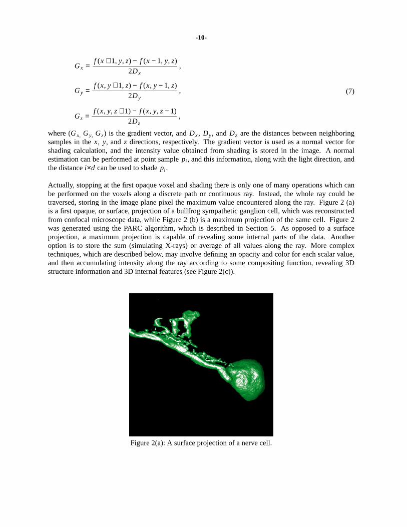
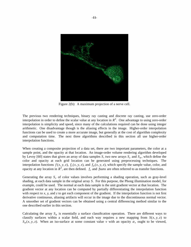
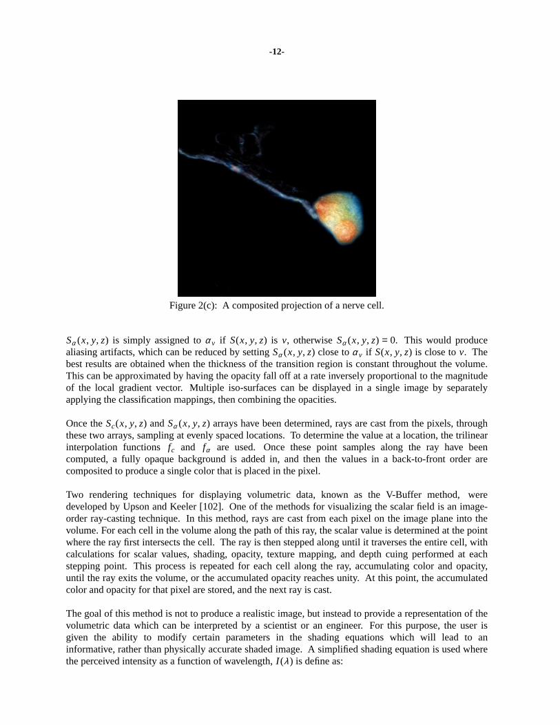
Actually, stopping at the first opaque voxel and shading there is only one of many operations which canbe performed on the voxels along a discrete path or continuous ray. Instead, the whole ray could betraversed, storing in the image plane pixel the maximum value encountered along the ray. Figure 2 (a)is a first opaque, or surface, projection of a bullfrog sympathetic ganglion cell, which was reconstructedfrom confocal microscope data, while Figure 2 (b) is a maximum projection of the same cell. Figure 2was generated using the PARC algorithm, which is described in Section 5. As opposed to a surfaceprojection, a maximum projection is capable of revealing some internal parts of the data. Anotheroption is to store the sum (simulating X-rays) or average of all values along the ray. More complextechniques, which are described below, may involve defining an opacity and color for each scalar value,and then accumulating intensity along the ray according to some compositing function, revealing 3Dstructure information and 3D internal features (see Figure 2(c)).

Figure 2(a): A surface projection of a nerve cell.

-11-

Figure 2(b): A maximum projection of a nerve cell.

The previous two rendering techniques, binary ray casting and discrete ray casting, use zero-orderinterpolation in order to define the scalar value at any location inR3. One advantage to using zero-orderinterpolation is simplicity and speed, since many of the calculations required can be done using integerarithmetic. One disadvantage though is the aliasing effects in the image. Higher-order interpolationfunctions can be used to create a more accurate image, but generally at the cost of algorithm complexityand computation time. The next three algorithms described in this section all use higher-orderinterpolation functions.

When creating a composite projection of a data set, there are two important parameters, the color at asample point, and the opacity at that location. An image-order volume rendering algorithm developedby Levo y [60] states that given an array of data samplesS, two new arraysSc andSα , which define thecolor and opacity at each grid location can be generated using preprocessing techniques. Theinterpolation functionsf (x, y, z), fc(x, y, z), and fα (x, y, z), which specify the sample value, color, andopacity at any location inR3, are then defined.fc and fsunxare often referred to as transfer functions.

Generating the arraySc of color values involves performing a shading operation, such as gray-levelshading, at each data sample in the original arrayS. For this purpose, the Phong illumination model, forexample, could be used. The normal at each data sample is the unit gradient vector at that location. Thegradient vector at any location can be computed by partially differentiating the interpolation functionwith respect tox, y,andz to get each component of the gradient. If the interpolation function is not firstderivative continuous, aliasing artifacts will occur in the image due to the discontinuous normal vector.A smoother set of gradient vectors can be obtained using a central differencing method similar to theone described earlier in this section.

Calculating the arraySα is essentially a surface classification operation. There are different ways toclassify surfaces within a scalar field, and each way requires a new mapping fromS(x, y, z) toSα (x, y, z). When an iso-surface at some constant valuev with an opacityα v ought to be viewed,

-12-

Figure 2(c): A composited projection of a nerve cell.

Sα (x, y, z) is simply assigned toα v if S(x, y, z) is v, otherwiseSα (x, y, z) = 0. This would producealiasing artifacts, which can be reduced by settingSα (x, y, z) close toα v if S(x, y, z) is close tov. Thebest results are obtained when the thickness of the transition region is constant throughout the volume.This can be approximated by having the opacity fall off at a rate inversely proportional to the magnitudeof the local gradient vector. Multiple iso-surfaces can be displayed in a single image by separatelyapplying the classification mappings, then combining the opacities.

Once theSc(x, y, z) andSα (x, y, z) arrays have been determined, rays are cast from the pixels, throughthese two arrays, sampling at evenly spaced locations. To determine the value at a location, the trilinearinterpolation functions fc and fα are used. Once these point samples along the ray have beencomputed, a fully opaque background is added in, and then the values in a back-to-front order arecomposited to produce a single color that is placed in the pixel.

Tw o rendering techniques for displaying volumetric data, known as the V-Buffer method, weredeveloped by Upson and Keeler [102]. One of the methods for visualizing the scalar field is an image-order ray-casting technique. In this method, rays are cast from each pixel on the image plane into thevolume. For each cell in the volume along the path of this ray, the scalar value is determined at the pointwhere the ray first intersects the cell. The ray is then stepped along until it traverses the entire cell, withcalculations for scalar values, shading, opacity, texture mapping, and depth cuing performed at eachstepping point. This process is repeated for each cell along the ray, accumulating color and opacity,until the ray exits the volume, or the accumulated opacity reaches unity. At this point, the accumulatedcolor and opacity for that pixel are stored, and the next ray is cast.

The goal of this method is not to produce a realistic image, but instead to provide a representation of thevolumetric data which can be interpreted by a scientist or an engineer. For this purpose, the user isgiven the ability to modify certain parameters in the shading equations which will lead to aninformative, rather than physically accurate shaded image. A simplified shading equation is used wherethe perceived intensity as a function of wav elength,I (λ) is define as:

-13-

(8)I (λ) = Ka(λ)I a + Kd(λ)j

Σ[(N ⋅ L j )I j ]

In this equation,Ka is the ambient coefficient,I a is the ambient intensity,Kd is the diffuse coefficient,N is the normal approximated by the local gradient,L j is the vector to thej th light source, andI j is theintensity of the j th light source. In order to highlight certain features in the final image, the diffusecoefficient can be defined as a function of not only wav elength, but also scalar value and solid texture:

(9)Kd(λ , S, M) = K (λ) Td(λ , S(x, y, z) M(λ , x, y, z)),

whereK is the actual diffuse coefficient,Td is the color transfer function,S is the sample array, andMis the solid texture map. The color transfer function is defined for red, green, and blue, and maps scalarvalue to intensity. In this method the following intensity integral is approximated when accumulatingalong the ray:

(10)I (λ) = ∫wτ (d)O(s)

Ka(λ)I a + Kd(λ , S, M) Σ

(N ⋅ L j )I j

+ (1 − τ (d)bc(λ))du

whereτ (d) represents atmospheric attenuation as a function of distanced, O (s) is the opacity transferfunction, bc is the background color, andu is a vector in the direction of the view ray. The opacitytransfer function is similar to the color transfer function in that it defines opacity as a function of scalarvalue. Different color and opacity transfer functions can be defined to highlight different features in thevolume.

The second method for visualizing the scalar field is a cell-by-cell processing technique [Upston Keeler1988.], where within each cell an image-order ray-casting technique is used, thus making this a hybridtechnique. In this method, each cell in the volume is processed in a front-to-back order. Processingbegins on the plane closest to the viewpoint, and progresses in a plane-by-plane manner. Within eachplane, processing begins with the cell closest to the viewpoint, then continues in order of increasingdistance from the viewpoint. Each cell is processed by first determining for each scan line in the imageplane, which pixels are affected by the cell. Then, for each pixel an integration volume is determined.Within the bounds of the integration volume, an intensity calculation similar to Equation 10 isperformed according to:

(11)I (λ) = ∫x ∫y ∫zτ (d)O(s)

Ka(λ)I a + Kd(λ , S, M) Σ

(N ⋅ L j )I j

+ (1 − τ (d)bc(λ))dxdydz

This process continues in a front-to-back order, until all cells have been processed, with intensityaccumulated into pixel values. Once a pixel opacity reaches unity, a flag is set and this pixel is notprocessed further. Due to the front-to-back nature of this algorithm, incremental display of the image ispossible.

In order to simulate light coming from translucent objects, volumetric data with data samplesrepresenting density values can be considered as a field of density emitters [84]. A density emitter is atiny particle that both emits and scatters light. The amount of density emitters in any small regionwithin the volume is proportional to the scalar value in that region. These density emitters are used tocorrectly model the occlusion of deeper parts of the volume by closer parts, but both shadowing andcolor variation due to differences in scattering at different wav elengths are ignored. These effects areignored because it is believed that they would complicate the image, detracting from the perception ofdensity variation. Similar to the V-Buffer method, rays are cast from the eye point, through each pixelon the image plane, and into the volume. The intensityI of light for a given pixel is calculatedaccording to:

-14-

(12)I =t2

t1∫ e

−τt

t1∫ ργ (λ)dλ

ργ (t)dt

In this equation, the ray is traversed fromt1 to t2, accumulating at each locationt the densityργ (t) at

that location attenuated by the probabilitye−τ

t

t1∫ ργ (λ)dλ

that this light will be scattered before reachingthe eye. The parameterτ is modifiable, and controls the attenuation, with higher values ofτ specifyinga medium which darkens more rapidly. The parameterγ is also modifiable, and controls the spread ofdensity values. Lowγ values produce a diffuse cloud appearance, while higherγ values highlight denseportions of the data. For each ray, three values in addition toI maybe computed. The maximum valueencountered along the ray, the distance at which that maximum occurred, and the center of gravity ofdensity emitters along the ray. By mapping these values to different color parameters (such as hue,saturation and lightness), interesting effects can be achieved. Krueger [55] showed that the variousexisting volume rendering models can be described as special cases of an underlying transport theorymodel of the transfer of particles in inhomogeneous media. The basic idea is that a beam of ‘‘virtual’’particles is sent through the volume, with the user selecting the particle properties and the laws ofinteraction between the particles and the data. The image plane then contains the ‘‘scattered’’ virtualparticles, and information about the data is obtained from the scattering pattern. If, for example, thevirtual particles are chosen to have the properties of photons, and the laws of interaction are governedby optical laws, then this model essentially becomes a generalized ray tracer. Other virtual particles andinteraction laws can be used, for example, to identify periodicities and similar hidden symmetries of thedata.

Using Krueger’s transport theory model, the intensity of lightI at a pixel can be described as a pathintegral along the view ray:

(13)I =pfar

pnear

∫ Q(p)e−

p

pnear

∫ σ a(p′)+σ pc(p′)d p′

dp

The emission at each pointp along the ray is scaled by the optical depth to the eye to produce the finalintensity value for a pixel. The optical depth is a function of the total extinction coefficient, which iscomposed of the absorption coefficientσ a, and the scattering coefficientσ sc. The generalized sourceQ(p) is defined as:

(14)Q(p) = q(p) + σ sc(p) ∫ ρ sc(→ω ′ → →ω )I (S, →ω ′)d →ω ′

This generalized source consists of the emission at a given pointq(p), and the incoming intensity alongall directions scaled by the scattering phaseρ sc. Typically, a low albedo approximation is used tosimplify the calculations, reducing the integral in Equation 15 to a sum over all light sources.

4.3. Domain Volume Rendering

In domain rendering the spatial 3D data is first transformed into another domain, such as compression,frequency, and wav elet domain, and then a projection is generated directly from that domain or with thehelp of information from that domain. The frequency domain rendering applies the Fourier sliceprojection theorem, which states that a projection of the 3D data volume from a certain view directioncan be obtained by extracting a 2D slice perpendicular to that view direction out of the 3D Fourier

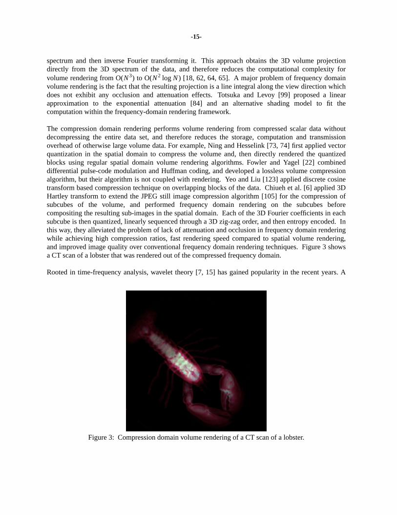
-15-

spectrum and then inverse Fourier transforming it. This approach obtains the 3D volume projectiondirectly from the 3D spectrum of the data, and therefore reduces the computational complexity forvolume rendering from O(N3) to O(N2 log N) [18, 62, 64, 65]. A major problem of frequency domainvolume rendering is the fact that the resulting projection is a line integral along the view direction whichdoes not exhibit any occlusion and attenuation effects. Totsuka and Levo y [99] proposed a linearapproximation to the exponential attenuation [84] and an alternative shading model to fit thecomputation within the frequency-domain rendering framework.

The compression domain rendering performs volume rendering from compressed scalar data withoutdecompressing the entire data set, and therefore reduces the storage, computation and transmissionoverhead of otherwise large volume data. For example, Ning and Hesselink [73, 74] first applied vectorquantization in the spatial domain to compress the volume and, then directly rendered the quantizedblocks using regular spatial domain volume rendering algorithms. Fowler and Yagel [22] combineddifferential pulse-code modulation and Huffman coding, and developed a lossless volume compressionalgorithm, but their algorithm is not coupled with rendering. Yeo and Liu [123] applied discrete cosinetransform based compression technique on overlapping blocks of the data. Chiueh et al. [6] applied 3DHartley transform to extend the JPEG still image compression algorithm [105] for the compression ofsubcubes of the volume, and performed frequency domain rendering on the subcubes beforecompositing the resulting sub-images in the spatial domain. Each of the 3D Fourier coefficients in eachsubcube is then quantized, linearly sequenced through a 3D zig-zag order, and then entropy encoded. Inthis way, they alleviated the problem of lack of attenuation and occlusion in frequency domain renderingwhile achieving high compression ratios, fast rendering speed compared to spatial volume rendering,and improved image quality over conventional frequency domain rendering techniques. Figure 3 showsa CT scan of a lobster that was rendered out of the compressed frequency domain.

Rooted in time-frequency analysis, wav elet theory [7, 15] has gained popularity in the recent years. A

Figure 3: Compression domain volume rendering of a CT scan of a lobster.

-16-

wavelet is a fast decaying function with zero averaging. The nice features of wav elets are that they hav elocal property in both spatial and frequency domain, and can be used to fully represent the volumes withsmall number of wav elet coefficients. Muraki [71] first applied wav elet transform to volumetric datasets, Gross et al. [30] found an approximate solution for the volume rendering equation usingorthonormal wav elet functions, and Westermann [110] combined volume rendering with wav elet-basedcompression. However, all of these algorithms have not focused on the acceleration of volume renderingusing wav elets. The greater potential of wav elet domain, based on the elegant multiresolution hierarchyprovided by the wav elet transform, is still far from fully utilized for volume rendering. A possibleresearch and development is to exploit the local frequency variance provided by wav elet transform andaccelerate the volume rendering in homogeneous area.

5. Volume Rendering Optimizations

Volume rendering can produce informative images that can be useful in data analysis, but a majordrawback of the techniques described above isthe time required to generate a high-quality image. Inthis section, several volume rendering optimizations are described that decrease rendering times, andtherefore increase interactivity and productivity. Other optimizations have been discussed briefly earlierin the paper, along with the original algorithms. Another way to speed up volume rendering is toemploy special-purpose hardware accelerators for volume rendering, which are described in Section 6.

Object-order volume rendering typically loops through the data, calculating the contribution of eachvolume sample to pixels on the image plane. This is a costly operation for moderate to large sized datasets (e.g., 128M bytes for a 5123 sample data set, with one byte per sample), leading to rendering timesthat are non-interactive. Viewing the intermediate results in the image plane may be useful, but thesepartial image results are not always representatives of the final image. For the purpose of interaction, itis useful to be able to generate a lower quality image in a shorter amount of time. For data sets withbinary sample values, bits could be packed into bytes such that each byte represents a 2×2×2 portion ofthe data [101]. The data would be processed bit by bit to generate the full resolution image, but lowerresolution image could be generated by processing the data byte by byte. If more than four bits of thebyte are set, the byte is considered to represent an element of the object, otherwise it represents thebackground. This will produce an image with one-half the linear resolution in approximately one-eighth the time.

A more general method for decreasing data resolution is to build a pyramid data structure, which for anoriginal data set ofN3 data samples, consists of a sequence of logN volumes. The first volume is theoriginal data set, while the second volume is created by averaging each 2×2×2 group of samples of theoriginal data set to create a volume of one-eight the resolution. The third volume is created from thesecond volume in a similar fashion, with this process continuing until all logN volumes have beencreated. An efficient implementation of the splatting algorithm, called hierarchical splatting [58], usessuch a pyramid data structure. According to the desired image quality, this algorithm scans theappropriate level of the pyramid in a back-to-front order. Each element is splatted onto the image planeusing the appropriate sized splat. The splats themselves are approximated by polygons which canefficiently be rendered by graphics hardware.

Image-order volume rendering involves casting rays from the image plane into the data, and samplingalong the ray in order to determine pixel values. The idea of pyramid can also be used here. Actually,Wang and Kaufman [108] have proposed the use of multi-resolution hierarchy at arbitrary resolutions.

-17-

In discrete ray casting, the ray would be discretized, and the contribution from each voxel along the pathis considered when producing the final pixel value. It would be quite computationally expensive todiscretize every ray cast from the image plane. Fortunately, this is unnecessary for parallel projections.Since all the rays are parallel, one ray can be discretized into a 26-connected line and used as a‘‘template’’ for all other rays. This technique, developed by Yagel and Kaufman [119], is calledtemplate-based volume viewing. If this template were used to cast a ray from each pixel in the imageplane, some voxels in the data may contribute to the image twice while others may not be considered atall. To solve this problem, the rays are cast instead from abaseplane, that is, the plane of the volumebuffer most parallel to the image plane. This ensures that each data sample can contribute at most onceto the final image, and all data samples could potentially contribute. Once all the rays have been castfrom the base plane, a simple final step of resampling is needed, which uses bilinear interpolation todetermine the pixel values on the image plane from the ray values that have been calculated on the baseplane.

An extension can be made to this template-based ray casting to allow higher-order interpolation [121].The template for higher-order interpolation consists of connected cells, as opposed to the connectedvoxel template used for zero-order interpolation. Since the value varies within a cell, it is desirable totake multiple samples along the continuous ray inside of each cell. Since these samples are taken atregular intervals, and the same template is used for every ray, there is only a finite number of 3Dlocations (relative to a cell) at which sampling occurs. This fact allows us to precompute part of theinterpolation function and store it in a table, allowing for faster rendering times.

Another extension to template-based ray casting allows for screen space supersampling to improveimage quality [118]. This is accomplished by allowing rays to originate at sub-pixel locations. A finitenumber of sub-pixel locations from which a ray can originate is selected, and a template is created foreach. When a ray is cast, its sub-pixel location determines which template is used. For example, toaccomplish a 2×2 uniform supersampling, four rays would be cast per pixel, and therefore four sub-pixel locations are possible. Stochastic supersampling can also be supported by limiting the possibleray origins to a finite number of sub-pixel locations, and precomputing a template for each.

Lacroute and Levo y [56] extended the previous ideas in an algorithm called shear-warp factorization. Itis based on algorithm that factors the viewing transformation into a 3D shear parallel to the data-slices, aprojection to form an intermediate but distorted image, and a 2D warp to form an undistorted finalimage. The algorithm is extended in three ways. First, a fast object-order rendering algorithm based onthe factorization algorithms with pre-processing and some loss of image quality, has been developed.Shear-warp factorization has the property that rows of voxels in the volume are aligned with rows ofpixels in the intermediate image. Consequently, a scanline-based algorithm has been constructed thattraverses the volume and the intermediate image in synchrony, taking advantage of the spatial coherencepresent in both. Spatial data structures based on run-length encoding for both the volume and theintermediate image are used. An implementation running on an SGI Indigo workstation renders a 2563

voxel data set in one second. The second extension is shear-warp factorization for perspective viewingtransformations. Third, a data structure for encoding spatial coherence in unclassified volumes (i.e.,scalar fields with no precomputed opacity) has been introduced. When combined with the shear-warprendering algorithm this data structure supports classification and rendering a 2563 voxel volume inthree seconds. The method extends to support mixed volumes and geometry and is parallelizable [57].

One obvious optimization for both discrete and continuous ray casting which has already been discussedis to limit the sampling to the segment of the ray which intersects the data, since samples outside of thedata evaluate to 0 and do not contribute to the pixel value. If the data itself contains many zero-valued

-18-

data samples, or a segmentation function is applied to the data that evaluates to 0 for many samples, theefficiency of ray casting can be greatly enhanced by further limiting the segment of the ray in whichsamples are taken. One algorithm of this sort is known aspolygon assisted ray casting, or PARC[1].This algorithm approximates objects contained within a volume using a crude polyhedral representation.The polyhedral representation is created so that it completely contains the objects. Using conventionalgraphics hardware, the polygons are projected twice to create two Z-buffers. The first Z-buffer is thestandard closest-distance Z-buffer, while the second is a farthest-distance Z-buffer. Since the object iscompletely contained within the representation, the two Z-buffer values for a given image plane pixelcan be used as the starting and ending points of a ray segment on which samples are taken.

The PARC algorithm is part of theVolVis volume visualization system [1, 2], which provides a multi-algorithm progressive refinement approach for interactivity. By using available graphics hardware, theuser is given the ability to interactively manipulate a polyhedral representation of the data. When theuser is satisfied with the placement of the data, light sources, and view, the Z-buffer information ispassed to the PARC algorithm, which produces a ray-cast image. In a final step, this image is furtherrefined by continuing to follow the PARC rays which intersected the data according to a volumetric raytracing algorithm [92] in order to generate shadows, reflections, and transparency (See Section 7.1).The ray tracing algorithm uses various optimization techniques, including uniform space subdivisionand bounding boxes, to increase the efficiency of the secondary rays. Surface rendering, as well astransparency with color and opacity transfer functions, are incorporated within a global illuminationmodel.

6. Special-Purpose Volume Rendering Hardware

The high computational cost of direct volume rendering makes it difficult for sequentialimplementations and general-purpose computers to deliver the targeted level of performance. Thissituation is aggravated by the continuing trend towards higher and higher resolution datasets. Forexample, to render a dataset of 10243 16-bit voxels at 30 frames per second requires 2 GBytes ofstorage, a memory transfer rate of 60 GBytes per second and approximately 300 billion instructions persecond, assuming 10 instructions per voxel per projection. To address this challenge, researchers havetried to achieve interactive display rates on supercomputers and massively parallel architectures [70, 86,104, 124]. However, most algorithms require very little repeated computation on each voxel and datamovement actually accounts for a significant portion of the overall performance overhead. Todayscommercial supercomputer memory systems don’t hav e and will not have in the near future adequatelatency and memory bandwidth for efficiently transferring the required large amounts of data.Furthermore, supercomputers seldom contain frame buffers and, due to their high cost, are frequentlyshared by many users.

The same way as the special requirements of traditional computer graphics lead to high-performancegraphics engines, volume visualization naturally lends itself to special-purpose volume renderers thatseparate real-time image generation from general-purpose processing. This allows for stand-alonevisualization environments that help scientists to interactively view their data on a single userworkstation, either augmented by a volume rendering accelerator or connected to a dedicatedvisualization server. Furthermore, a volume rendering engine integrated in a graphics workstation is anatural extension of raster based systems into 3D volume visualization.

Several researchers have proposed special-purpose volume rendering architectures [49, Chapter 6] [27,

-19-

41, 47, 68, 76, 95, 96, 116]. Most recent research focuses on accelerators for ray-casting of regulardatasets. Ray-casting offers room for algorithmic improvements while still allowing for high imagequality. Recent architectures [37] include VOGUE, VIRIM, and Cube.

VOGUE [54], a modular add-on accelerator, is estimated to achieve 2.5 frames per second for 2563

datasets. For each pixel a ray is defined by the host computer and sent to the accelerator. The VOGUEmodule autonomously processes the complete ray, consisting of evenly spaced resampling locations, andreturns the final pixel color of that ray to the host. Several VOGUE modules can be combined to yieldhigher performance implementations. For example, to achieve 20 projections per second of 5123

datasets requires 64 boards and a 5.2 GB per second ring-connected cubic network.

VIRIM [31] is a flexible and programmable ray-casting engine. The hardware consists of two separateunits, the first being responsible for 3D resampling of the volume using lookup tables to implementdifferent interpolation schemes. The second unit performs the ray-casting through the resampled datasetaccording to user programmable lighting and viewing parameters. The underlying ray-casting modelallows for arbitrary parallel and perspective projections and shadows. An existing hardwareimplementation for the visualization of 256× 256× 128 datasets at 10 frames per second requires 16processing boards.

The Cube project aims at the realization of high-performance volume rendering systems for largedatasets and pioneered several hardware architectures. Cube-1, a first generation hardware prototype,was based on a specially interleaved memory organization [46], which has also been used in allsubsequent generations of the Cube architecture. This interleaving of then3 voxel enables conflict-freeaccess to any ray parallel to a main axis ofn voxels. A fully operational printed circuit board (PCB)implementation of Cube-1 is capable of generating orthographic projections of 163 datasets from a finitenumber of predetermined directions in real-time. Cube-2 was a single-chip VLSI implementation ofthis prototype [3].

To achieve higher performance and to further reduce the critical memory access bottleneck, Cube-3introduced several new concepts [78-80]. A high-speed global communication network aligns anddistributes voxels from the memory to several parallel processing units and a circular cross-linkedbinary tree of voxel combination units composites all samples into the final pixel color. Estimatedperformance for arbitrary parallel and perspective projections is 30 frames per second for 5123 datasets.Cube-4 [81] has only simple and local interconnections, thereby allowing for easy scalability ofperformance. Instead of processing individual rays, Cube-4 manipulates a group of rays at a time. As aresult, the rendering pipeline is directly connected to the memory. Accumulating compositors replacethe binary compositing tree. A pixel-bus collects and aligns the pixel output from the compositors.Cube-4 is easily scalable to very high resolution of 10243 16-bit voxels and true real-time performanceimplementations of 30 frames per second.

The choice of whether one adopts a general-purpose or a special-purpose solution to volume renderingdepends upon the circumstances. If maximum flexibility is required, general-purpose appears to be thebest way to proceed. However, an important feature of graphics accelerators is that they are integratedinto a much larger environment where software can shape the form of input and output data, therebyproviding the additional flexibility that is needed. A good example is the relationship between the needsof conventional computer graphics and special-purpose graphics hardware. Nobody would dispute thenecessity for polygon graphics acceleration despite its obvious limitations. The exact same argumentcan be made for special-purpose volume rendering architectures.

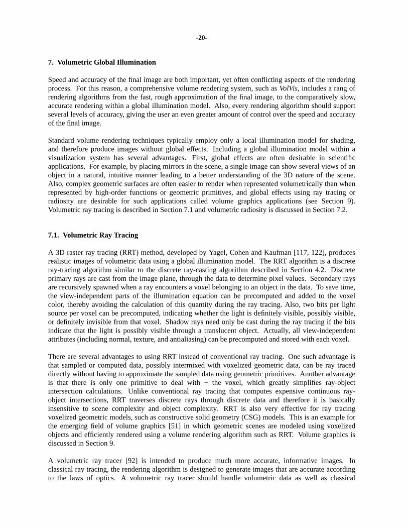
-20-

7. Volumetric Global Illumination

Speed and accuracy of the final image are both important, yet often conflicting aspects of the renderingprocess. For this reason, a comprehensive volume rendering system, such asVolVis, includes a rang ofrendering algorithms from the fast, rough approximation of the final image, to the comparatively slow,accurate rendering within a global illumination model. Also, every rendering algorithm should supportseveral levels of accuracy, giving the user an even greater amount of control over the speed and accuracyof the final image.

Standard volume rendering techniques typically employ only a local illumination model for shading,and therefore produce images without global effects. Including a global illumination model within avisualization system has several advantages. First, global effects are often desirable in scientificapplications. For example, by placing mirrors in the scene, a single image can show sev eral views of anobject in a natural, intuitive manner leading to a better understanding of the 3D nature of the scene.Also, complex geometric surfaces are often easier to render when represented volumetrically than whenrepresented by high-order functions or geometric primitives, and global effects using ray tracing orradiosity are desirable for such applications called volume graphics applications (see Section 9).Volumetric ray tracing is described in Section 7.1 and volumetric radiosity is discussed in Section 7.2.

7.1. Volumetric Ray Tracing

A 3D raster ray tracing (RRT) method, developed by Yagel, Cohen and Kaufman [117, 122], producesrealistic images of volumetric data using a global illumination model. The RRT algorithm is a discreteray-tracing algorithm similar to the discrete ray-casting algorithm described in Section 4.2. Discreteprimary rays are cast from the image plane, through the data to determine pixel values. Secondary raysare recursively spawned when a ray encounters a voxel belonging to an object in the data. To sav e time,the view-independent parts of the illumination equation can be precomputed and added to the voxelcolor, thereby avoiding the calculation of this quantity during the ray tracing. Also, two bits per lightsource per voxel can be precomputed, indicating whether the light is definitely visible, possibly visible,or definitely invisible from that voxel. Shadow rays need only be cast during the ray tracing if the bitsindicate that the light is possibly visible through a translucent object. Actually, all view-independentattributes (including normal, texture, and antialiasing) can be precomputed and stored with each voxel.

There are several advantages to using RRT instead of conventional ray tracing. One such advantage isthat sampled or computed data, possibly intermixed with voxelized geometric data, can be ray traceddirectly without having to approximate the sampled data using geometric primitives. Another advantageis that there is only one primitive to deal with − the voxel, which greatly simplifies ray-objectintersection calculations. Unlike conventional ray tracing that computes expensive continuous ray-object intersections, RRT traverses discrete rays through discrete data and therefore it is basicallyinsensitive to scene complexity and object complexity. RRT is also very effective for ray tracingvoxelized geometric models, such as constructive solid geometry (CSG) models. This is an example forthe emerging field of volume graphics [51] in which geometric scenes are modeled using voxelizedobjects and efficiently rendered using a volume rendering algorithm such as RRT. Volume graphics isdiscussed in Section 9.

A volumetric ray tracer [92] is intended to produce much more accurate, informative images. Inclassical ray tracing, the rendering algorithm is designed to generate images that are accurate accordingto the laws of optics. A volumetric ray tracer should handle volumetric data as well as classical

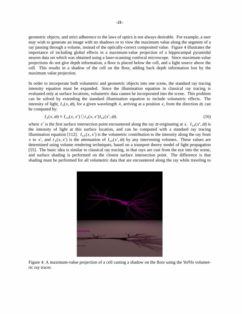
-21-

geometric objects, and strict adherence to the laws of optics is not always desirable. For example, a usermay wish to generate an image with no shadows or to view the maximum value along the segment of aray passing through a volume, instead of the optically-correct composited value. Figure 4 illustrates theimportance of including global effects in a maximum-value projection of a hippocampal pyramidalneuron data set which was obtained using a laser-scanning confocal microscope. Since maximum-valueprojections do not give depth information, a floor is placed below the cell, and a light source above thecell. This results in a shadow of the cell on the floor, adding back depth information lost by themaximum value projection.

In order to incorporate both volumetric and geometric objects into one scene, the standard ray tracingintensity equation must be expanded. Since the illumination equation in classical ray tracing isevaluated only at surface locations, volumetric data cannot be incorporated into the scene. This problemcan be solved by extending the standard illumination equation to include volumetric effects. Theintensity of light,I λ (x, →ω ), for a given wav elengthλ , arriving at a positionx, from the direction→ω , canbe computed by:

(16)I λ (x, →ω ) = I vλ (x, x′) + τ λ (x, x′)I sλ (x′, →ω ).

wherex′ is the first surface intersection point encountered along the ray→ω originating atx. I sλ (x′, →ω ) isthe intensity of light at this surface location, and can be computed with a standard ray tracingillumination equation [112].I vλ (x, x′) is the volumetric contribution to the intensity along the ray fromx to x′, andτ λ (x, x′) is the attenuation ofI sλ (x′, →ω ) by any intervening volumes. These values aredetermined using volume rendering techniques, based on a transport theory model of light propagation[55]. The basic idea is similar to classical ray tracing, in that rays are cast from the eye into the scene,and surface shading is performed on the closest surface intersection point. The difference is thatshading must be performed for all volumetric data that are encountered along the ray while traveling to

Figure 4: A maximum-value projection of a cell casting a shadow on the floor using theVolVisvolumet-ric ray tracer.

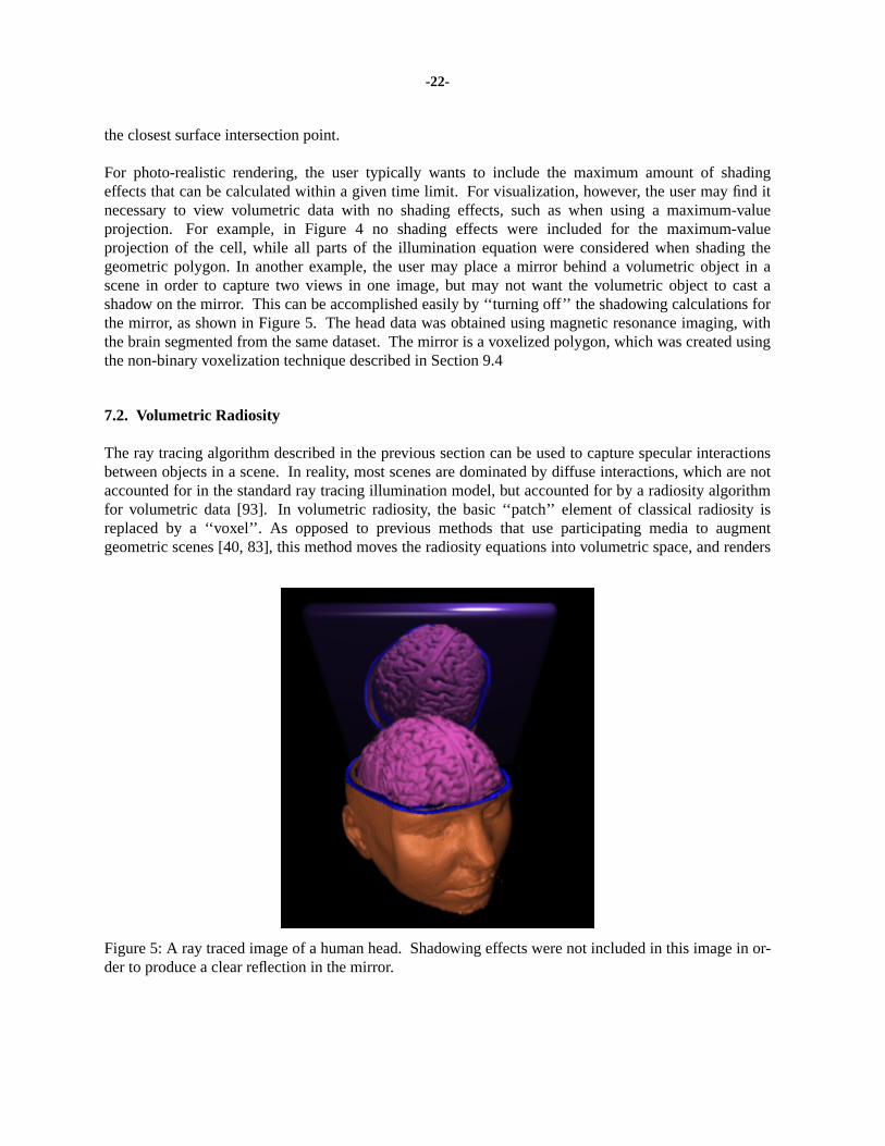
-22-

the closest surface intersection point.

For photo-realistic rendering, the user typically wants to include the maximum amount of shadingeffects that can be calculated within a given time limit. For visualization, however, the user may find itnecessary to view volumetric data with no shading effects, such as when using a maximum-valueprojection. For example, in Figure 4 no shading effects were included for the maximum-valueprojection of the cell, while all parts of the illumination equation were considered when shading thegeometric polygon. In another example, the user may place a mirror behind a volumetric object in ascene in order to capture two views in one image, but may not want the volumetric object to cast ashadow on the mirror. This can be accomplished easily by ‘‘turning off’’ the shadowing calculations forthe mirror, as shown in Figure 5. The head data was obtained using magnetic resonance imaging, withthe brain segmented from the same dataset. The mirror is a voxelized polygon, which was created usingthe non-binary voxelization technique described in Section 9.4

7.2. Volumetric Radiosity

The ray tracing algorithm described in the previous section can be used to capture specular interactionsbetween objects in a scene. In reality, most scenes are dominated by diffuse interactions, which are notaccounted for in the standard ray tracing illumination model, but accounted for by a radiosity algorithmfor volumetric data [93]. In volumetric radiosity, the basic ‘‘patch’’ element of classical radiosity isreplaced by a ‘‘voxel’’. As opposed to previous methods that use participating media to augmentgeometric scenes [40, 83], this method moves the radiosity equations into volumetric space, and renders

Figure 5: A ray traced image of a human head. Shadowing effects were not included in this image in or-der to produce a clear reflection in the mirror.

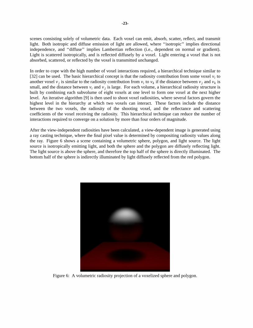
-23-

scenes consisting solely of volumetric data. Each voxel can emit, absorb, scatter, reflect, and transmitlight. Both isotropic and diffuse emission of light are allowed, where ‘‘isotropic’’ implies directionalindependence, and ‘‘diffuse’’ implies Lambertian reflection (i.e., dependent on normal or gradient).Light is scattered isotropically, and is reflected diffusely by a voxel. Light entering a voxel that is notabsorbed, scattered, or reflected by the voxel is transmitted unchanged.

In order to cope with the high number of voxel interactions required, a hierarchical technique similar to[32] can be used. The basic hierarchical concept is that the radiosity contribution from some voxelvi toanother voxelv j is similar to the radiosity contribution fromvi to vk if the distance betweenv j andvk issmall, and the distance betweenvi andv j is large. For each volume, a hierarchical radiosity structure isbuilt by combining each subvolume of eight voxels at one level to form one voxel at the next higherlevel. An iterative algorithm [9] is then used to shoot voxel radiosities, where several factors govern thehighest level in the hierarchy at which two voxels can interact. These factors include the distancebetween the two voxels, the radiosity of the shooting voxel, and the reflectance and scatteringcoefficients of the voxel receiving the radiosity. This hierarchical technique can reduce the number ofinteractions required to converge on a solution by more than four orders of magnitude.

After the view-independent radiosities have been calculated, a view-dependent image is generated usinga ray casting technique, where the final pixel value is determined by compositing radiosity values alongthe ray. Figure 6 shows a scene containing a volumetric sphere, polygon, and light source. The lightsource is isotropically emitting light, and both the sphere and the polygon are diffusely reflecting light.The light source is above the sphere, and therefore the top half of the sphere is directly illuminated. Thebottom half of the sphere is indirectly illuminated by light diffusely reflected from the red polygon.

Figure 6: A volumetric radiosity projection of a voxelized sphere and polygon.

-24-

8. Irregular Grid Rendering

All the algorithms discussed above handle only regular gridded data. Irregular gridded data comes in alarge variety [94], including curvilinear data or unstructured (scattered) data, where no explicitconnectivity is defined between cells (one can even be giv en a scattered collection of points that can beturned into an irregular grid by interpolation [66, 72]). For rendering purposes, manifold (locallyhomeomorphic toR3) grids composed of convex cells are usually necessary. In general, the mostconvenient grids for rendering purposes are tetrahedral grids and hexahedral grids. One disadvantage ofhexahedral grids is that the four points on the side of a cell may not necessarily lie on a plane forcing therendering algorithm to approximate the cells by convex ones during rendering. Tetrahedral grids haveseveral advantages, including easier interpolation, simple representation (specially for connectivityinformation because the degree of the connectivity graph is bounded, allowing for compact datastructure representation), and the fact that any other grid can be interpolated to a tetrahedral one (withthe possible introduction of Steiner points). Among their disadvantages is the fact that the size of thedatasets tend to grow as cells are decomposed into tetrahedra. In the case of curvilinear grids, anaccurate (and naive) decomposition will make the cell complex contain five times as many cells.

As compared to regular grids, operations for irregular grids are more complicated and the effectivevisualization methods are more sophisticated in all fronts. Shading, interpolation, point location, etc.,are all harder (and some even not well defined) for irregular grids. One notable exception is isosurfacegeneration [63], that even in the case of irregular grids is fairly simple to compute given suitableinterpolation functions. Slicing operations are also simple [94].

Volume rendering irregular grids is a hard operation and there are several different approaches to thisproblem. The simplest and most inefficient is to resample the irregular grid to a regular grid. In order toachieve the necessary accuracy, a high enough sampling rate has to be used what in most cases willmake the resulting regular grid volume too large for storage and rendering purposes, not mentioning thetime to perform the re-sampling.

Extending the simple volumetric point sampling ray tracing to irregular grids is a challenge. For raytracing, it is necessary to depth-sort samples along ray emanating from each screen pixel. In the case ofirregular grids, it is not trivial to perform this sorting operation. Garrity [24] proposed a scheme wherethe cells are convex and connectivity information is available. He proposed to pre-process the gridfinding the external cells to help locating the boundary elements during ray tracing, and using theconnectivity information for cell skipping. The actual resampling and shading, that is simple in theregular grid, is not trivial here and has to be carefully considered, usually taking into account thespecific application at hand (actually the development of accurate illumination models for volumerendering has irregular grid rendering as one of its main uses [67]). Simple ray casting is too inefficient,as there is a large amount of inter-pixel and inter-scanline coherency in ray casting. Giertsen [25]proposed a sweep-plane approach to ray casting that uses different forms of "caching" to speed up raycasting irregular grids.

Another approach for rendering irregular grids is the use of feed-forward (or projection) methods, wherethe cells are projected onto the screen one by one accumulating their contributions incrementally to thefinal image [66, 89, 113, 114]. One major advantage of these methods is the ability to use the graphicshardware on graphics workstations to compute the volumetric lighting models (usually simplified) inorder to speed up rendering. Another advantage is that the user can see the rendering as it progresses.One problem with this method is generating the ordering for the cell projections. In general, suchordering does not even exist and cells have to be partitioned into multiple cells for projection. The

-25-

partitioning is (in general) view dependent, but some types of irregular grids (like delaunaytriangulations in space) are acyclic and do not need any partitioning.

9. Volume Graphics

The 3D raster representation seems to be more natural for empirical imagery then for geometric objects,due to its ability to represent interiors and digital samples. Nonetheless, the advantages of thisrepresentation are also attracting traditional surface-based applications that deal with the modeling andrendering of synthetic scenes made out of geometric models. The geometric model isvoxelized (3Dscan-converted)into a set of voxels that ‘‘best’’ approximate the model. Each of these voxels is thenstored in the volume buffer together with the voxel pre-computed view-independent attributes. Thevoxelized model can be either binary (see [10, 43-45]) or volume sampled [106] which generates alias-free density voxelization of the model. Some surface-based application examples are the rendering offractals [75], hyper textures [77], fur [42], gases [20], and other complex models [90] including CADmodels and terrain models for flight simulators [11, 51, 115]. Furthermore, in many applicationsinvolving sampled data, such as medial imaging, the data need to be visualized along with syntheticobjects that may not be available in digital form, such as scalpels, prosthetic devices, injection needles,radiation beams, and isodose surfaces. These geometric objects can be voxelized and intermixed withthe sampled organ in the voxel buffer [48].

Volume graphics[51], which is an emerging subfield of computer graphics, is concerned with thesynthesis, modeling, manipulation, and rendering of volumetric geometric objects, stored in a volumebuffer of voxels. Unlike volume visualization which focuses primarily on sampled and computeddatasets, volume graphics is concerned primarily with modeled geometric scenes and commonly withthose that are represented in a regular volume buffer. As an approach, volume graphics has the potentialto greatly advance the field of 3D graphics by offering a comprehensive alternative to traditional surfacegraphics.

In the next sub-sections we describe the volumetric approach to several common volume graphicsmodeling techniques. We describe the generation of object primitives (voxelization), 3D antialiasing,texture and photo mapping, solid-texturing, modeling of amorphous phenomena, modeling by blockoperations, constructive solid modeling, and volume sculpting. Then, volume graphics is contrastedwith surface graphics, and the corresponding advantages are discussed.

9.1. Voxelization

An indispensable stage in volume graphics is the synthesis of voxel-represented objects from theirgeometric representation. This stage, which is calledvoxelization, is concerned with convertinggeometric objects from their continuous geometric representation into a set of voxels that ‘‘best’’approximates the continuous object. As this process mimics the scan-conversion process that pixelizes(rasterizes) 2D geometric objects, it is also referred to as3D scan-conversion. In 2D rasterization thepixels are directly drawn onto the screen to be visualized and filtering is applied to reduce the aliasingartifacts. However, the voxelization process does not render the voxels but merely generates a databaseof the discrete digitization of the continuous object.

Intuitively, one would assume that a proper voxelization simply ‘‘selects’’ all voxels which are met (if

-26-

only partially) by the object body. Although this approach could be satisfactory in some cases, theobjects it generates are commonly too coarse and include more voxels than are necessary. For example,when a 2D curve is rasterized into a connected sequence of pixels, the discrete curve does not ‘‘cover’’the entire continuous curve, but it is connected and concisely and successfully ‘‘separates’’ both ‘‘sides’’of the curve [12].

One practical meaning of separation is apparent when a voxelized scene is rendered by casting discreterays from the image plane to the scene. The penetration of the background voxels (which simulate thediscrete ray traversal) through the voxelized surface causes the appearance of a hole in the final image ofthe rendered surface. Another type of error might occur when a 3D flooding algorithm is employedeither to fill an object or to measure its volume, surface area, or other properties. In this case thenonseparability of the surface causes a leakage of the flood through the discrete surface.

Unfortunately, the extension of the 2D definition of separation to the third dimension and to voxelsurfaces is not straightforward since voxelized surfaces cannot be defined as an ordered sequence ofvoxels and a voxel on the surface does not have a specific number of adjacent surface voxels.Furthermore, there are important topological issues, such as the separation of both sides of a surface,which cannot be well-defined by employing 2D terminology. The theory that deals with thesetopological issues is called3D discrete topology. We sketch below some basic notions and informaldefinitions used in this field.

9.2. Fundamentals of 3D Discrete Topology

The 3D discrete space is a set of integral grid points in 3D Euclidean space defined by their Cartesiancoordinates (x, y, z). A voxel is the unit cubic volume centered at the integral grid point. The voxelvalue is mapped onto 0,1: the voxels assigned ‘‘1’’ are called the ‘‘black’’ voxels representing opaqueobjects, and those assigned ‘‘0’’ are the ‘‘white’’ voxels representing the transparent background. InSection 9.4 we describe non-binary approaches where the voxel value is mapped onto the interval [0,1]representing either partial coverage, variable densities, or graded opacities. Due to its larger dynamicrange of values, this approach supports 3D antialiasing and thus supports higher quality rendering.

Tw o voxels are26-adjacentif they share either a vertex, an edge, or a face (see Figure 1). Every voxelhas 26 such adjacent voxels: eight share a vertex (corner) with the center voxel, twelve share an edge,and six share a face. Accordingly, face-sharing voxels are defined as6-adjacent, and edge-sharing andface-sharing voxels are defined as18-adjacent. The prefixN is used to define the adjacency relation,whereN = 6, 18, or 26. A sequence of voxels having the same value (e.g., ‘‘black’’) is called anN-pathif all consecutive pairs areN-adjacent. A set of voxelsW is N-connectedif there is anN-path betweenev ery pair of voxels inW. An N-connected componentis a maximalN-connected set.

Given a 2D discrete 8-connected black curve, there are sequences of 8-connected white pixels(8-component) that pass from one side of the black component to its other side without intersecting it.This phenomenon is a discrete disagreement with the continuous case where there is no way ofpenetrating a closed curve without intersecting it. To avoid such a scenario, it has been the conventionto define ‘‘opposite’’ types of connectivity for the white and black sets. ‘‘Opposite’’ types in 2D spaceare 4 and 8, while in 3D space 6 is ‘‘opposite’’ to 26 or to 18.

Assume that a voxel space, denoted byΣ, includes one subset of ‘‘black’’ voxelsS. If Σ − S is not N-connected, that is,Σ − S consists of at least two whiteN-connected components, thenS is said to beN-

-27-

separatingin Σ. Loosely speaking, in 2D, an 8-connected black path that divides the white pixels intotwo groups is 4-separating and a 4-connected black path that divides the white pixels into two groups is8-separating. There are no analogous results in 3D space.

Let W be anN-separating surface. A voxelp ∈ W is said to be anN-simple voxelif W − p is still N-separating. AnN-separating surface is calledN-minimal if it does not contain anyN-simple voxel. Acoverof a continuous surface is a set of voxels such that every point of the continuous surface lies in avoxel of the cover. A cover is said to be aminimal coverif none of its subsets is also a cover. The coverproperty is essential in applications that employ space subdivision for fast ray tracing [26]. Thesubspaces (voxels) which contain objects have to be identified along the traced ray. Note that a cover isnot necessarily separating, while on the other hand, as mentioned above, it may include simple voxels.In fact, even a minimal cover is not necessarilyN-minimal for anyN [12].

9.3. Binary Voxelization

An early technique for the digitization of solids was spatial enumeration which employs point or cellclassification methods in either an exhaustive fashion or by recursive subdivision [59]. However,subdivision techniques for model decomposition into rectangular subspaces are computationallyexpensive and thus inappropriate for medium or high resolution grids. Instead, objects should bedirectly voxelized, preferably generating anN-separating,N-minimal, and covering set, whereN isapplication dependent. The voxelization algorithms should follow the same paradigm as the 2D scan-conversion algorithms; they should be incremental, accurate, use simple arithmetic (preferably integeronly), and have a complexity that is not more than linear with the number of voxels generated.

The literature of 3D scan-conversion is relatively small. Danielsson [14] and Mokrzycki [69] developedindependently similar 3D curve algorithms where the curve is defined by the intersection of two implicitsurfaces. Voxelization algorithms have been developed for 3D lines, 3D circles, and a variety ofsurfaces and solids, including polygons, polyhedra, and quadric objects [43]. Efficient algorithms havebeen developed for voxelizing polygons using an integer-based decision mechanism embedded within ascan-line filling algorithm [44], for parametric curves, surfaces, and volumes using an integer-basedforward differencing technique [45], and for quadric objects such as cylinders, spheres, and cones using‘‘weaving’’ algorithms by which a discrete circle/line sweeps along a discrete circle/line [10]. Figure 7consists of a variety of objects (polygons, boxes, cylinders) voxelized using these methods. Thesepioneering attempts should now be followed by enhanced voxelization algorithms that, in addition tobeing efficient and accurate, will also adhere to the topological requirements of separation, coverage,and minimality.

9.4. 3D Antialiasing

The previous sub-section discussed binary voxelization, which generate topologically and geometricallyconsistent models, but exhibit object space aliasing. These algorithms have used a straightforwardmethod of sampling in space, calledpoint sampling. In point sampling, the continuous object isevaluated at the voxel center, and the value of 0 or 1 is assigned to the voxel. Because of this binaryclassification of the voxels, the resolution of the 3D raster ultimately determines the precision of thediscrete model. Imprecise modeling results in jagged surfaces, known asobject space aliasing(seeFigure 7). In this section, a 3D object-space antialiasing technique is presented. It performs antialiasingonce, on a 3D view-independent representation, as part of the modeling stage. Unlike antialiasing of 2D

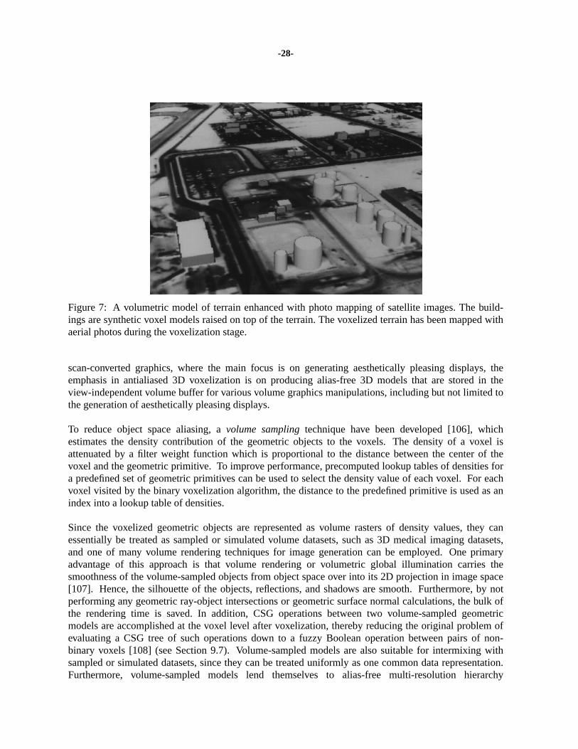
-28-

Figure 7: A volumetric model of terrain enhanced with photo mapping of satellite images. The build-ings are synthetic voxel models raised on top of the terrain. The voxelized terrain has been mapped withaerial photos during the voxelization stage.

scan-converted graphics, where the main focus is on generating aesthetically pleasing displays, theemphasis in antialiased 3D voxelization is on producing alias-free 3D models that are stored in theview-independent volume buffer for various volume graphics manipulations, including but not limited tothe generation of aesthetically pleasing displays.

To reduce object space aliasing, avolume samplingtechnique have been developed [106], whichestimates the density contribution of the geometric objects to the voxels. The density of a voxel isattenuated by a filter weight function which is proportional to the distance between the center of thevoxel and the geometric primitive. To improve performance, precomputed lookup tables of densities fora predefined set of geometric primitives can be used to select the density value of each voxel. For eachvoxel visited by the binary voxelization algorithm, the distance to the predefined primitive is used as anindex into a lookup table of densities.

Since the voxelized geometric objects are represented as volume rasters of density values, they canessentially be treated as sampled or simulated volume datasets, such as 3D medical imaging datasets,and one of many volume rendering techniques for image generation can be employed. One primaryadvantage of this approach is that volume rendering or volumetric global illumination carries thesmoothness of the volume-sampled objects from object space over into its 2D projection in image space[107]. Hence, the silhouette of the objects, reflections, and shadows are smooth. Furthermore, by notperforming any geometric ray-object intersections or geometric surface normal calculations, the bulk ofthe rendering time is saved. In addition, CSG operations between two volume-sampled geometricmodels are accomplished at the voxel level after voxelization, thereby reducing the original problem ofevaluating a CSG tree of such operations down to a fuzzy Boolean operation between pairs of non-binary voxels [108] (see Section 9.7). Volume-sampled models are also suitable for intermixing withsampled or simulated datasets, since they can be treated uniformly as one common data representation.Furthermore, volume-sampled models lend themselves to alias-free multi-resolution hierarchy

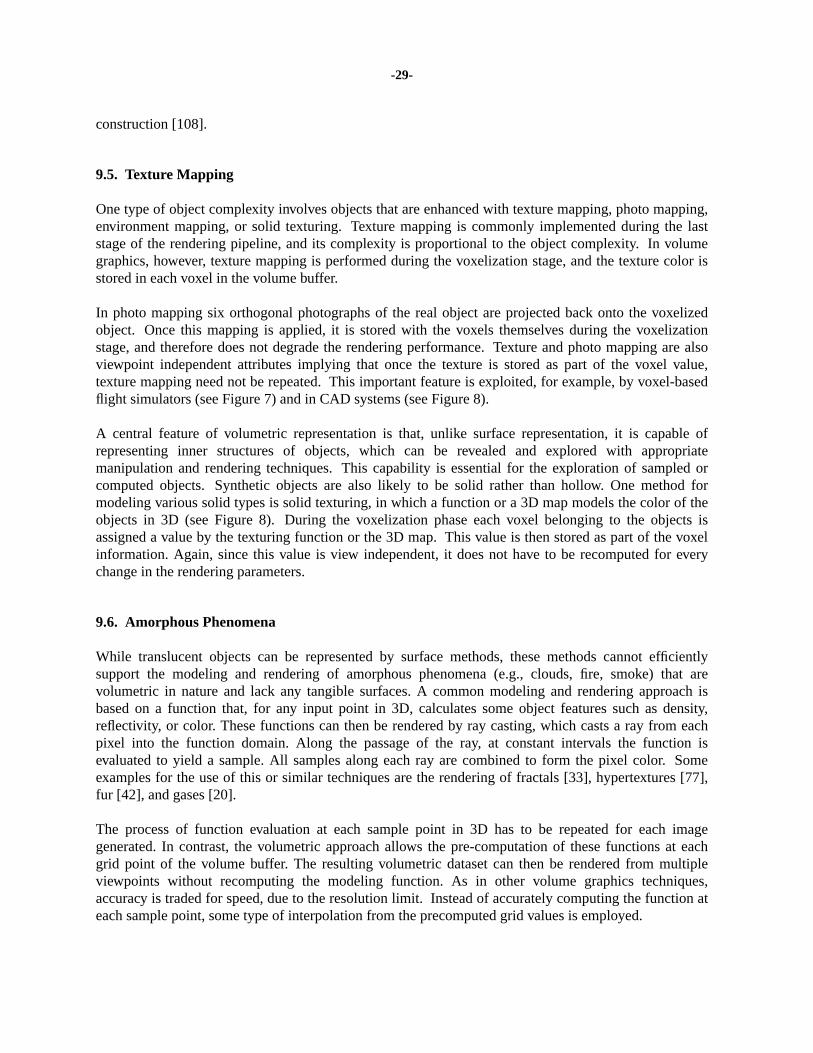
-29-

construction [108].

9.5. Texture Mapping

One type of object complexity involves objects that are enhanced with texture mapping, photo mapping,environment mapping, or solid texturing. Texture mapping is commonly implemented during the laststage of the rendering pipeline, and its complexity is proportional to the object complexity. In volumegraphics, however, texture mapping is performed during the voxelization stage, and the texture color isstored in each voxel in the volume buffer.

In photo mapping six orthogonal photographs of the real object are projected back onto the voxelizedobject. Once this mapping is applied, it is stored with the voxels themselves during the voxelizationstage, and therefore does not degrade the rendering performance. Te xture and photo mapping are alsoviewpoint independent attributes implying that once the texture is stored as part of the voxel value,texture mapping need not be repeated. This important feature is exploited, for example, by voxel-basedflight simulators (see Figure 7) and in CAD systems (see Figure 8).

A central feature of volumetric representation is that, unlike surface representation, it is capable ofrepresenting inner structures of objects, which can be revealed and explored with appropriatemanipulation and rendering techniques. This capability is essential for the exploration of sampled orcomputed objects. Synthetic objects are also likely to be solid rather than hollow. One method formodeling various solid types is solid texturing, in which a function or a 3D map models the color of theobjects in 3D (see Figure 8). During the voxelization phase each voxel belonging to the objects isassigned a value by the texturing function or the 3D map. This value is then stored as part of the voxelinformation. Again, since this value is view independent, it does not have to be recomputed for everychange in the rendering parameters.

9.6. Amorphous Phenomena

While translucent objects can be represented by surface methods, these methods cannot efficientlysupport the modeling and rendering of amorphous phenomena (e.g., clouds, fire, smoke) that arevolumetric in nature and lack any tangible surfaces. A common modeling and rendering approach isbased on a function that, for any input point in 3D, calculates some object features such as density,reflectivity, or color. These functions can then be rendered by ray casting, which casts a ray from eachpixel into the function domain. Along the passage of the ray, at constant intervals the function isevaluated to yield a sample. All samples along each ray are combined to form the pixel color. Someexamples for the use of this or similar techniques are the rendering of fractals [33], hypertextures [77],fur [42], and gases [20].

The process of function evaluation at each sample point in 3D has to be repeated for each imagegenerated. In contrast, the volumetric approach allows the pre-computation of these functions at eachgrid point of the volume buffer. The resulting volumetric dataset can then be rendered from multipleviewpoints without recomputing the modeling function. As in other volume graphics techniques,accuracy is traded for speed, due to the resolution limit. Instead of accurately computing the function ateach sample point, some type of interpolation from the precomputed grid values is employed.

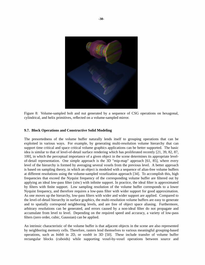
-30-

Figure 8: Volume-sampled bolt and nut generated by a sequence of CSG operations on hexagonal,cylindrical, and helix primitives, reflected on a volume-sampled mirror.

9.7. Block Operations and Constructive Solid Modeling

The presortedness of the volume buffer naturally lends itself to grouping operations that can beexploited in various ways. For example, by generating multi-resolution volume hierarchy that cansupport time critical and space critical volume graphics applications can be better supported. The basicidea is similar to that of level-of-detail surface rendering which has proliferated recently [21, 39, 82, 87,100], in which the perceptual importance of a given object in the scene determines its appropriate level-of-detail representation. One simple approach is the 3D "mip-map" approach [61, 85], where everylevel of the hierarchy is formed by averaging several voxels from the previous level. A better approachis based on sampling theory, in which an object is modeled with a sequence of alias-free volume buffersat different resolutions using the volume-sampled voxelization approach [34]. To accomplish this, highfrequencies that exceed the Nyquist frequency of the corresponding volume buffer are filtered out byapplying an ideal low-pass filter (sinc) with infinite support. In practice, the ideal filter is approximatedby filters with finite support. Low sampling resolution of the volume buffer corresponds to a lowerNyquist frequency, and therefore requires a low-pass filter with wider support for good approximation.As one moves up the hierarchy, low-pass filters with wider and wider support are applied. Compared tothe level-of-detail hierarchy in surface graphics, the multi-resolution volume buffers are easy to generateand to spatially correspond neighboring levels, and are free of object space aliasing. Furthermore,arbitrary resolutions can be generated, and errors caused by a non-ideal filter do not propagate andaccumulate from level to lev el. Depending on the required speed and accuracy, a variety of low-passfilters (zero order, cubic, Gaussian) can be applied.

An intrinsic characteristic of the volume buffer is that adjacent objects in the scene are also representedby neighboring memory cells. Therefore, rasters lend themselves to various meaningful grouping-basedoperations, such asbitblt in 2D, or voxblt in 3D [50]. These include transfer of volume bufferrectangular blocks (cuboids) while supporting voxel-by-voxel operations between source and

-31-

destination blocks. Block operations add a variety of modeling capabilities which aid in the task ofimage synthesis and form the basis for the efficient implementation of a 3D ‘‘room manager’’, which isthe extension of window management to the third dimension.

Since the volume buffer lends itself to Boolean operations that can be performed on a voxel-by-voxelbasis during the voxelization stage, it is advantageous to use CSG as the modeling paradigm.Subtraction, union, and intersection operations between two voxelized objects are accomplished at thevoxel lev el, thereby reducing the original problem of evaluating a CSG tree during rendering time downto a 1D Boolean operation between pairs of voxels during a preprocessing stage.

For two point-sampled binary objects the Boolean operations of CSG orvoxblt are trivially defined.However, the Boolean operations applied to volume-sampled models are analogous to those of fuzzy settheory (cf. [17]). The volume-sampled model is a density functiond(x) over R3, whered is 1 inside theobject, 0 outside the object, and 0 <d < 1 within the "soft" region of the filtered surface. Some of thecommon operations, intersection, complement, difference, and union, between two objectsA andB aredefined as follows:

(17)dA∩ B(x) ≡ min ( dA(x), dB(x))

(18)dA(x) ≡ 1 − dA(x)

(19)dA−B(x) ≡ min (dA(x), 1 − dB(x))

(20)dA∪ B(x) ≡ max (dA(x), dB(x))

The only law of set theory that is no longer true is the excluded-middle law (i.e.,A ∩ A ≠ φ andA ∪ A ≠ Universe). The use of the min and max functions causes discontinuity at the region where thesoft regions of the two objects meet, since the density value at each location in the region is determinedsolely by one of the two overlapping objects.

Complex geometric models can be generated by performing the CSG operations in Equations 17-20between volume-sampled primitives. Volume-sampled models can also function as matte volumes [16]for various matting operations, such as performing cut-aways and merging multiple volumes into asingle volume using the union operation. However, in order to preserve continuity on the cut-awayboundaries between the material and the empty space, one should use an alternative set of Booleanoperators based on algebraic sum and algebraic product [17, 28] :

(21)dA∩ B(x) ≡ dA(x) dB(x)

(22)dA(x) ≡ 1 − dA(x)

(23)dA−B(x) ≡ dA(x) − dA(x) dB(x)

(24)dA∪ B(x) ≡ dA(x) + dB(x) − dA(x) dB(x)

Unlike the min and max operators, algebraic sum and product operators result inA ∪ A ≠ A, which isundesirable. A consequence, for example, is that during modeling via sweeping, the resulting model issensitive to the sampling rate of the swept path [108].

Once a CSG model has been constructed in voxel representation, it is rendered in the same way anyother volume buffer is. This makes, for example, volumetric ray tracing of constructive solid modelsstraightforward [92] (see Figure 8).

-32-

9.8. Volume Sculpting

Surface-based sculpting has been studied extensively (e.g., [13, 88]), while volume sculpting has beenrecently introduced for clay or wax-like sculptures [23] and for comprehensive detailed sculpting [109].The latter approach is a free-form interactive modeling technique based on the metaphor of sculptingand painting a voxel-based solid material, such as a block of marble or wood. There are twomotivations for this approach. First, modeling topologically complex and highly-detailed objects arestill difficult in most CAD systems. Second, sculpting has shown to be useful in volumetricapplications. For example, scientists and physicians often need to explore the inner structures of theirsimulated or sampled datasets by gradually removing material.

Real-time human interaction could be achieved in this approach, since the actions of sculpting (e.g.,carving, sawing) and painting are localized in the volume buffer, a localized rendering can be employedto reproject only those pixels that are affected. Carving is the process of taking a pre-existing volume-sampled tool to chip or chisel the object bit by bit. Since both the object and the tool are represented asindependent volume buffers, the process of sculpting involves positioning the tool with respect to theobject and performing a Boolean subtraction between the two volumes. Sawing is the process ofremoving a whole chunk of material at once, much like a carpenter sawing off a portion of a woodpiece. Unlike carving, sawing requires generating the volume-sampled tool on-the-fly, using a userinterface. To prevent object space aliasing and to achieve interactive speed, 3D splatting is employed.

9.9. Surface Graphics vs. Volume Graphics

Contemporary 3D graphics has been employing an object-based approach at the expense of maintainingand manipulating a display list of geometric objects and regenerating the frame-buffer after everychange in the scene or viewing parameters. This approach, termedsurface graphics, is supported bypowerful geometry engines, which have flourished in the past decade, making surface graphics the state-of-the-art in 3D graphics.

Surface graphics strikingly resembles vector graphics that prevailed in the sixties and seventies, andemployed vector drawing devices. Like vector graphics, surface graphics represents the scene as a set ofgeometric primitives kept in a display list. In surface graphics, these primitives are transformed,mapped to screen coordinates, and converted by scan-conversion algorithms into a discrete set of pixels.Any change to the scene, viewing parameters, or shading parameters requires the image generationsystem to repeat this process. Like vector graphics that did not support painting the interior of 2Dobjects, surface graphics generates merely the surfaces of 3D objects and does not support the renderingof their interior.

Instead of a list of geometric objects maintained by surface graphics, volume graphics employs a 3Dvolume buffer as a medium for the representation and manipulation of 3D scenes. A 3D scene isdiscretized earlier in the image generation sequence, and the resulting 3D discrete form is used as adatabase of the scene for manipulation and rendering purposes, which in effect decouples discretizationfrom rendering. Furthermore, all objects are converted into one uniform meta-object − the voxel. Eachvoxel is atomic and represents the information about at most one object that resides in that voxel.

Volume graphics offers similar benefits to surface graphics, with several advantages that are due to thedecoupling, uniformity, and atomicity features. The rendering phase is viewpoint independent andinsensitive to scene complexity and object complexity. It supports Boolean and block operations and

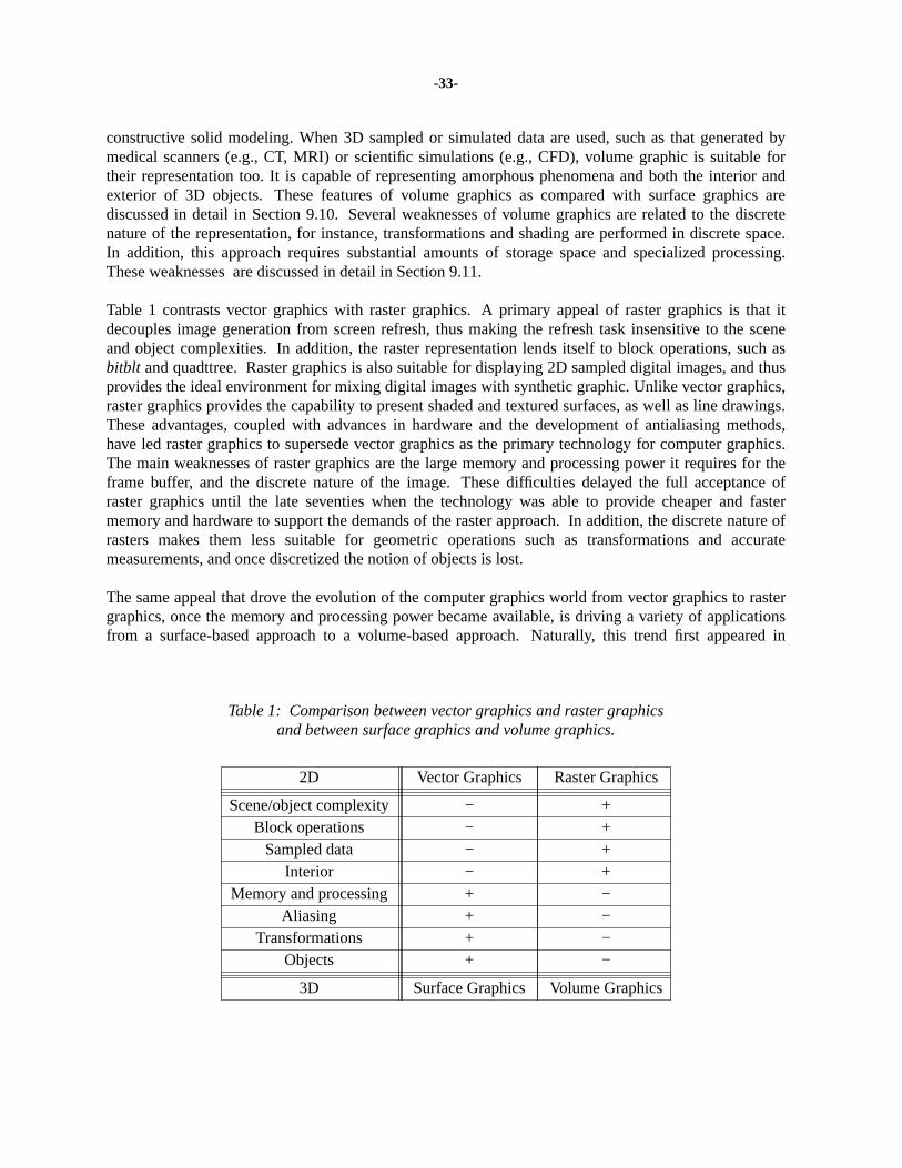
-33-

constructive solid modeling. When 3D sampled or simulated data are used, such as that generated bymedical scanners (e.g., CT, MRI) or scientific simulations (e.g., CFD), volume graphic is suitable fortheir representation too. It is capable of representing amorphous phenomena and both the interior andexterior of 3D objects. These features of volume graphics as compared with surface graphics arediscussed in detail in Section 9.10. Several weaknesses of volume graphics are related to the discretenature of the representation, for instance, transformations and shading are performed in discrete space.In addition, this approach requires substantial amounts of storage space and specialized processing.These weaknesses are discussed in detail in Section 9.11.

Table 1 contrasts vector graphics with raster graphics. A primary appeal of raster graphics is that itdecouples image generation from screen refresh, thus making the refresh task insensitive to the sceneand object complexities. In addition, the raster representation lends itself to block operations, such asbitblt and quadttree. Raster graphics is also suitable for displaying 2D sampled digital images, and thusprovides the ideal environment for mixing digital images with synthetic graphic. Unlike vector graphics,raster graphics provides the capability to present shaded and textured surfaces, as well as line drawings.These advantages, coupled with advances in hardware and the development of antialiasing methods,have led raster graphics to supersede vector graphics as the primary technology for computer graphics.The main weaknesses of raster graphics are the large memory and processing power it requires for theframe buffer, and the discrete nature of the image. These difficulties delayed the full acceptance ofraster graphics until the late seventies when the technology was able to provide cheaper and fastermemory and hardware to support the demands of the raster approach. In addition, the discrete nature ofrasters makes them less suitable for geometric operations such as transformations and accuratemeasurements, and once discretized the notion of objects is lost.

The same appeal that drove the evolution of the computer graphics world from vector graphics to rastergraphics, once the memory and processing power became available, is driving a variety of applicationsfrom a surface-based approach to a volume-based approach. Naturally, this trend first appeared in

Table 1: Comparison between vector graphics and raster graphicsand between surface graphics and volume graphics.

2D Vector Graphics Raster Graphics

Scene/object complexity − +Block operations − +

Sampled data − +Interior − +

Memory and processing + −Aliasing + −

Transformations + −Objects + −

3D Surface Graphics Volume Graphics

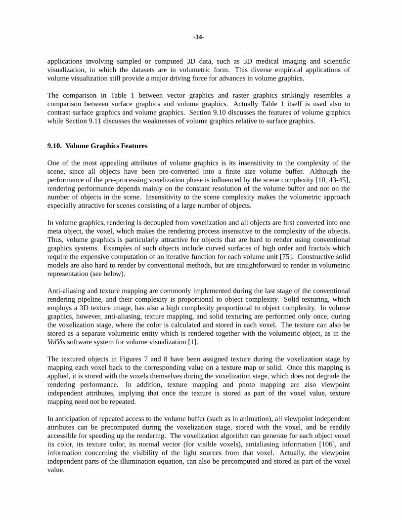
-34-

applications involving sampled or computed 3D data, such as 3D medical imaging and scientificvisualization, in which the datasets are in volumetric form. This diverse empirical applications ofvolume visualization still provide a major driving force for advances in volume graphics.

The comparison in Table 1 between vector graphics and raster graphics strikingly resembles acomparison between surface graphics and volume graphics. Actually Table 1 itself is used also tocontrast surface graphics and volume graphics. Section 9.10 discusses the features of volume graphicswhile Section 9.11 discusses the weaknesses of volume graphics relative to surface graphics.

9.10. Volume Graphics Features

One of the most appealing attributes of volume graphics is its insensitivity to the complexity of thescene, since all objects have been pre-converted into a finite size volume buffer. Although theperformance of the pre-processing voxelization phase is influenced by the scene complexity [10, 43-45],rendering performance depends mainly on the constant resolution of the volume buffer and not on thenumber of objects in the scene. Insensitivity to the scene complexity makes the volumetric approachespecially attractive for scenes consisting of a large number of objects.

In volume graphics, rendering is decoupled from voxelization and all objects are first converted into onemeta object, the voxel, which makes the rendering process insensitive to the complexity of the objects.Thus, volume graphics is particularly attractive for objects that are hard to render using conventionalgraphics systems. Examples of such objects include curved surfaces of high order and fractals whichrequire the expensive computation of an iterative function for each volume unit [75]. Constructive solidmodels are also hard to render by conventional methods, but are straightforward to render in volumetricrepresentation (see below).

Anti-aliasing and texture mapping are commonly implemented during the last stage of the conventionalrendering pipeline, and their complexity is proportional to object complexity. Solid texturing, whichemploys a 3D texture image, has also a high complexity proportional to object complexity. In volumegraphics, however, anti-aliasing, texture mapping, and solid texturing are performed only once, duringthe voxelization stage, where the color is calculated and stored in each voxel. The texture can also bestored as a separate volumetric entity which is rendered together with the volumetric object, as in theVolVissoftware system for volume visualization [1].

The textured objects in Figures 7 and 8 have been assigned texture during the voxelization stage bymapping each voxel back to the corresponding value on a texture map or solid. Once this mapping isapplied, it is stored with the voxels themselves during the voxelization stage, which does not degrade therendering performance. In addition, texture mapping and photo mapping are also viewpointindependent attributes, implying that once the texture is stored as part of the voxel value, texturemapping need not be repeated.

In anticipation of repeated access to the volume buffer (such as in animation), all viewpoint independentattributes can be precomputed during the voxelization stage, stored with the voxel, and be readilyaccessible for speeding up the rendering. The voxelization algorithm can generate for each object voxelits color, its texture color, its normal vector (for visible voxels), antialiasing information [106], andinformation concerning the visibility of the light sources from that voxel. Actually, the viewpointindependent parts of the illumination equation, can also be precomputed and stored as part of the voxelvalue.

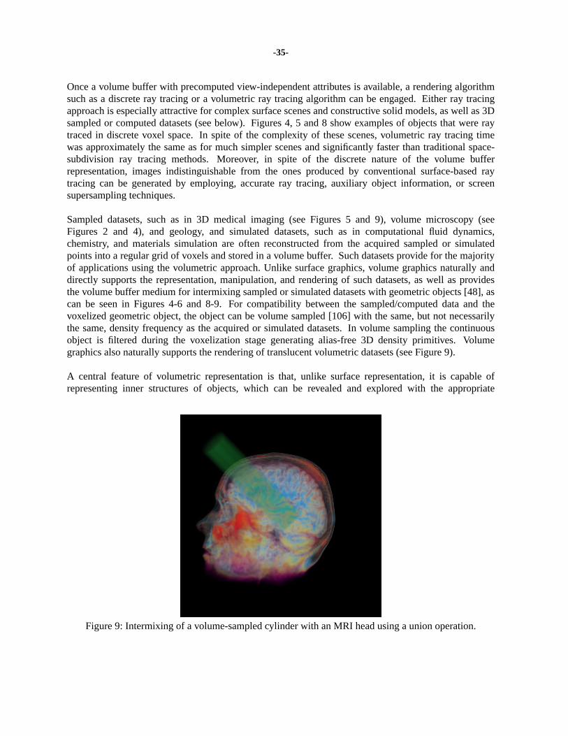
-35-

Once a volume buffer with precomputed view-independent attributes is available, a rendering algorithmsuch as a discrete ray tracing or a volumetric ray tracing algorithm can be engaged. Either ray tracingapproach is especially attractive for complex surface scenes and constructive solid models, as well as 3Dsampled or computed datasets (see below). Figures 4, 5 and 8 show examples of objects that were raytraced in discrete voxel space. In spite of the complexity of these scenes, volumetric ray tracing timewas approximately the same as for much simpler scenes and significantly faster than traditional space-subdivision ray tracing methods. Moreover, in spite of the discrete nature of the volume bufferrepresentation, images indistinguishable from the ones produced by conventional surface-based raytracing can be generated by employing, accurate ray tracing, auxiliary object information, or screensupersampling techniques.

Sampled datasets, such as in 3D medical imaging (see Figures 5 and 9), volume microscopy (seeFigures 2 and 4), and geology, and simulated datasets, such as in computational fluid dynamics,chemistry, and materials simulation are often reconstructed from the acquired sampled or simulatedpoints into a regular grid of voxels and stored in a volume buffer. Such datasets provide for the majorityof applications using the volumetric approach. Unlike surface graphics, volume graphics naturally anddirectly supports the representation, manipulation, and rendering of such datasets, as well as providesthe volume buffer medium for intermixing sampled or simulated datasets with geometric objects [48], ascan be seen in Figures 4-6 and 8-9. For compatibility between the sampled/computed data and thevoxelized geometric object, the object can be volume sampled [106] with the same, but not necessarilythe same, density frequency as the acquired or simulated datasets. In volume sampling the continuousobject is filtered during the voxelization stage generating alias-free 3D density primitives. Volumegraphics also naturally supports the rendering of translucent volumetric datasets (see Figure 9).

A central feature of volumetric representation is that, unlike surface representation, it is capable ofrepresenting inner structures of objects, which can be revealed and explored with the appropriate

Figure 9: Intermixing of a volume-sampled cylinder with an MRI head using a union operation.

-36-

volumetric manipulation and rendering techniques. Natural objects as well as synthetic objects arelikely to be solid rather than hollow. The inner structure is easily explored using volume graphics andcannot be supported by surface graphics (see Figures 2(b), 2(c), 3-6 and 9). Moreover, while translucentobjects can be represented by surface methods, these methods cannot efficiently support the translucentrendering of volumetric objects, or the modeling and rendering of amorphous phenomena (e.g., clouds,fire, smoke) that are volumetric in nature and do not contain any tangible surfaces [20, 42, 77].

An intrinsic characteristic of rasters is that adjacent objects in the scene are also represented byneighboring voxels. Therefore, rasters lend themselves to various meaningful block-based operationswhich can be performed during the voxelization stage. For example, the 3D counterpart of thebitbltoperations, termedvoxblt (voxel block-transfer), can support transfer of cuboidal voxel blocks with avariety of voxel-by-voxel operations between source and destination blocks [50]. This property is veryuseful for voxblt and CSG. Once a CSG model has been constructed in voxel representation, it isrendered like any other volume buffer. This makes rendering of constructive solid modelsstraightforward.

The spatial presortedness of the volume buffer voxels lends itself to other types of grouping oraggregation of neighboring voxels. For example, the terrain image shown in Figure 7 was generated bythe voxel-based Hughes Aircraft Co. flight simulator [115]. It simulates a flight over voxel-representedterrain enhanced with satellite or aerial photo mapping with additional synthetic raised objects, such asbuildings, trees, vehicles, aircraft, clouds and the like. Since the information below the terrain surface isinvisible, terrain voxels can be actually represented as tall cuboids extending from sea level to the terrainheight. The raised and moving objects, however, hav e to be represented in a more conventional voxel-based form.

Similarly, voxels can be aggregated into super-voxels in a pyramid-like hierarchy. For example, in avoxel-based flight simulator, the best resolution can be used for takeoff and landing. As the aircraftascends, fewer and fewer details need to be processed and visualized, and a lower resolution suffices.Furthermore, even in the same view, parts of the terrain close to the observer are rendered at highresolution which deceases towards the horizon. A hierarchical volume buffer can be prepared in advanceor on-the-fly by subsampling or averaging the appropriate size neighborhoods of voxels (see also [34]).

9.11. Weaknesses of Volume Graphics

A typical volume buffer occupies a large amount of memory. For example, for a medium resolution of5123, two bytes per voxel, the volume buffer consists of 256M bytes. However, since computermemories are significantly decreasing in price and increasing in their compactness and speed, such largememories are becoming common place. This argument echoes a similar discussion when rastergraphics emerged as a technology in the mid-seventies. With the rapid progress in memory price andcompactness, it is safe to predict that, as in the case of raster graphics, the memory will soon cease to bea stumbling block for volume graphics.

The extremely large throughput that has to be handled requires a special architecture and processingattention (see [49] Chapter 6).Volume engines, analogous to the currently available geometry (polygon)engines, are emerging. Because of the presortedness of the volume buffer and the fact that only a simplesingle type of object has to be handled, volume engines are conceptually simpler to implement thancurrent geometry engines (see Section 6). We predict that, consequently, volume engines willmaterialize in the near future, with capabilities to synthesize, load, store, manipulate, and render

-37-

volumetric scenes in real time (e.g., 30 frames/sec), configured possibly as accelerators or co-systems toexisting geometry engines.

Unlike surface graphics, in volume graphics the 3D scene is represented in discrete form. This is thecause of many of the problems of voxel-based graphics, which are similar to those of 2D rasters [19].The finite resolution of the raster poses a limit on the accuracy of some operations, such as volume andarea measurements, that are based on voxel counting.

Since the discrete data is sampled during rendering, a low resolution volume yields high aliasingartifacts. This becomes especially apparent when zooming in on the 3D raster. When naive renderingalgorithms are used, holes may appear "between" voxels. Nevertheless, this can be alleviated in wayssimilar to those adopted by 2D raster graphics, such as employing either reconstruction techniques, ahigher-resolution volume buffer, or volume sampling.

Manipulation and transformation of the discrete volume are difficult to achieve without degrading theimage quality or losing some information. Rotation of rasters by angles other than 90 degrees isespecially problematic since a sequence of consecutive rotations will distort the image. Again, thesecan be alleviated in ways similar to the 2D raster techniques.

Once an object has been voxelized, the voxels comprising the discrete object do not retain anygeometric information regarding the geometric definition of the object. Thus, it is advantageous, whenexact measurements are required (e.g., distance, area), to employ conventional modeling where thegeometric definition of the object is available. A voxel-based object is only a discrete approximation ofthe original continuous object where the volume buffer resolution determines the precision of suchmeasurements. On the other hand, several measurement types are more easily computed in voxel space(e.g., mass property, adjacency detection, and volume computation).

The lack of geometric information in the voxel may inflict other difficulties, such as surface normalcomputation. In voxel-based models, a discrete shading method is commonly employed to estimate thenormal from a context of voxels. A variety of image-based and object-based methods for normalestimation from volumetric data has been devised (see [120], [49, Chapter 4]) and some have beendiscussed above. Most methods are based on fitting some type of a surface primitive to a smallneighborhood of voxels.

A partial integration between surface and volume graphics is conceivable as part of an object-basedapproach in which an auxiliary object table, consisting of the geometric definition and global attributesof each object, is maintained in addition to the volume buffer. Each voxel consists of an index to theobject table. This allows exact calculation of normal, exact measurements, and intersection verificationfor discrete ray tracing [122]. The auxiliary geometric information might be useful also for re-voxelizing the scene in case of a change in the scene itself.

10. Conclusions

Many of the important concepts and computational methods of volume visualization have beenpresented. Surface rendering algorithms for volume data were briefly described in which anintermediate representation of the data is used to generate an image of a surface contained within thedata. Object order, image order, and domain volume rendering techniques were presented forgenerating images of surfaces within the data, as well as volume rendered images that attempt to capture

-38-

all three dimensions of information in the 2D image. Several optimization techniques that aim atdecreasing the rendering time for volume visualization as well as realistic global illumination renderingwere also described.

Although volumetric representations and visualization techniques seem more natural for sampled orcomputed data sets, their advantages are also attracting traditional geometric-based applications. Thistrend implies an expanding role for volume visualization, and it has thus the potential to revolutionizethe field of computer graphics, by providing an alternative to surface graphics, called volume graphics.We hav e introduced recent trends in volume visualization that brought about the emergence of volumegraphics. As summarized in Table 1, volume graphics has advantages over surface graphics by beingviewpoint independent, insensitive to scene and object complexity, and it lends itself to the realization ofblock operations, CSG modeling, and hierarchical representation. It is suitable for the representation ofsampled or simulated datasets and their intermixing with geometric objects, and it supports thevisualization of internal structures. The problems associated with the volume buffer representation,such as memory size, processing time, aliasing, and lack of geometric representation, echo problemsencountered when raster graphics emerged as an alternative technology to vector graphics and can bealleviated in similar ways.

The progress so far in volume graphics, in computer hardware, and memory systems, coupled with thedesire to reveal the inner structures of volumetric objects, suggests that volume visualization andvolume graphics may develop into major trends in computer graphics. Just as raster graphics in theseventies superseded vector graphics for visualizing surfaces, volume graphics has the potential tosupersede surface graphics for handling and visualizing volumes as well as for modeling and renderingsynthetic scenes composed of surfaces.

Acknowledgments

Special thanks are due to Lisa Sobierajski, Rick Avila, Roni Yagel, Dany Cohen, Sid Wang, TaosongHe, Hanspeter Pfister, and Lichan Hong who contributed to this paper, co-authored with me relatedpapers [2, 51-53], and helped with theVolVis software. (VolVis can be obtained by sending email to:volvis@cs.sunysb.edu.) This work has been supported by the National Science Foundation under grantsCCR-9205047 and MIP-9527694, and a grant from the Department of Energy under PICS grant. TheMRI head data in Figures 4 and 9 is courtesy of Siemens Medical Systems, Inc., Iselin, NJ. Figure 7 iscourtesy of Hughes Aircraft Company, Long Beach, CA. This image has been voxelized usingvoxelization algorithms, a voxel-based modeler, and a photo-mapper developed at Stony BrookVisualization Lab. The confocal microscope data in Figures 2 and 4 are courtesy of Howard HughesMedical Institute at Stony Brook, NY. The CT lobster data in Figure 5 is courtesy of AVS, Waltham,MA.

11. References

1. Avila, R., Sobierajski, L. and Kaufman, A., ‘‘Tow ards a Comprehensive Volume VisualizationSystem’’,Visualization ’92 Proceedings, October 1992, 13-20.

2. Avila, R., He, T., Hong, L., Kaufman, A., Pfister, H., Silva, C., Sobierajski, L. and Wang, S.,‘‘VolVis: A Diversified Volume Visualization System’’, Visualization ’94 Proceedings,Washington, DC, October 1994, 31-38.

3. Bakalash, R., Kaufman, A., Pacheco, R. and Pfister, H., ‘‘An Extended Volume VisualizationSystem for Arbitrary Parallel Projection’’,Proceedings of the 1992 Eurographics Workshop on

-39-

Graphics Hardware, Cambridge, UK, September 1992.

4. Barillot, C., Gibaud, B., Luo, L. M. and Scarabin, I. M., ‘‘3D Representation of AnatomicStructures From CT Examinations’’,Proceedings SPIE, 602, (1985), 307-314.

5. Chen, L. S., Herman, G. T., Reynolds, R. A. and Udupa, J. K., ‘‘Surface Shading in the CuberilleEnvironment’’,IEEE Computer Graphics & Applications, 5, 12 (December 1985), 33-43.

6. Chiueh, T., He, T., Kaufman, A. and Pfister, H., ‘‘Compression Domain Volume Rendering’’,Technical Report 94.01.04, Computer Science, SUNY at Stony Brook, January 1994.

7. Chui, C.,An Introduction to Wavelets, Academic Press, 1992.

8. Cline, H. E., Lorensen, W. E., Ludke, S., Crawford, C. R. and Teeter, B. C., ‘‘Two Algorithms forthe Three-Dimensional Reconstruction of Tomograms’’,Medical Physics, 15, 3 (May/June 1988),320-327.

9. Cohen, M. F., Chen, S. E., Wallace, J. R. and Greenberg, D. P., ‘‘A Progressive RefinementApproach to Fast Radiosity Image Generation’’,Computer Graphics (Proc SIGGRAPH), 1988,75-84.

10. Cohen, D. and Kaufman, A., ‘‘Scan Conversion Algorithms for Linear and Quadratic Objects’’, inVolume Visualization, A. Kaufman, (ed.), IEEE Computer Society Press, Los Alamitos, CA, 1991,280-301.

11. Cohen, D. and Shaked, A., ‘‘Photo-Realistic Imaging of Digital Terrain’’,Computer GraphicsForum, 12, 3 (September 1993), 363-374.

12. Cohen-Or, D. and Kaufman, A., ‘‘Fundamentals of Surface Voxelization’’,CVGIP: GraphicsModels and Image Processing, 56, 6 (November 1995), 453-461.

13. Coquillart, S., ‘‘Extended Free-Form Deformation: A Sculpturing Tool for 3D GeometricModeling’’, Computer Graphics, 24, 4 (August 1990), 187-196.

14. Danielsson, P. E., ‘‘Incremental Curve Generation’’,IEEE Transactions on Computers, C-19,(1970), 783-793.

15. Daubechies, I.,Ten Lectures on Wavelets, CBMS-NSF Regional Conference Series in AppliedMathematics, SIAM, 1992.

16. Drebin, R. A., Carpenter, L. and Hanrahan, P., ‘‘Volume Rendering’’,Computer Graphics (Proc.SIGGRAPH), 22, 4 (August 1988), 65-74.

17. Dubois, D. and Prade, H.,Fuzzy Sets and Systems: Theory and Applications, Academic Press,1980.

18. Dunne, S., Napel, S. and Rutt, B., ‘‘Fast Reprojection of Volume Data’’,Proceedings of the 1stConference on Visualization in Biomedical Computing, Atlanta, GA, 1990, 11-18.

19. Eastman, C. M., ‘‘Vector versus Raster: A Functional Comarison of Drawing Technologies’’,IEEE Computer Graphics & Applications, 10, 5 (September 1990), 68-80.

20. Ebert, D. S. and Parent, R. E., ‘‘Rendering and Animation of Gaseous Phenomena by CombiningFast Volume and Scanline A-buffer Techniques’’,Computer Graphics, 24, 4 (August 1990),357-366.

21. Eck, M., DeRose, T., Duchamp, T., Hoppe, H., Lounsbery, M. and Stuetzle, W., ‘‘MultiresolutionAnalysis of Arbitrary Meshes’’,SIGGRAPH’95 Conference Proceedings, August 1995, 173-182.

22. Fowler, J. and Yagel, R., ‘‘Lossless Compression of Volume Data’’,Proceedings Symposium onVolume Visualization, Washington, DC, October 1994, 43-50.

-40-

23. Galyean, T. A. and Hughes, J. F., ‘‘Sculpting: An Interactive Volumetric Medeling Technique’’,Computer Graphics, 25, 4 (July 1991), 267-274.

24. Garrity, M. P., ‘‘Raytracing Irregular Volume Data’’,Computer Graphics, 24, 5 (November 1990),35-40.

25. Giertsen, C., ‘‘Volume Visualization of Sparse Irregular Meshes’’,IEEE Computer Graphics &Applications, 12, 2 (March 1992), 40-48.

26. Glassner, A. S., ‘‘Space Subdivision for Fast Ray Tracing’’,IEEE Computer Graphics andApplications, 4, 10 (October 1984), 15-22.

27. Goldwasser, S. M., Reynolds, R. A., Bapty, T., Baraff, D., Summers, J., Talton, D. A. and Walsh,E., ‘‘Physician’s Workstation with Real-Time Performance’’,IEEE Computer Graphics &Applications, 5, 12 (December 1985), 44-57.

28. Goodman, J. R. and Sequin, C. H., ‘‘Hypertree: A Multiprocessor Interconnection Topology’’,IEEE Transactions on Computers, C-30, 12 (December 1981), 923-933.

29. Gordon, D. and Reynolds, R. A., ‘‘Image Space Shading of 3-Dimensional Objects’’,ComputerVision, Graphics and Image Processing, 29, (1985), 361-376.

30. Gross, M. H., Koch, R., Lippert, L. and Dreger, A., ‘‘A New Method to Approximate the VolumeRendering Equation using Wav elet Bases and Piecewise Polynomials’’,Computers & Graphics,19, 1 (1995), 47-62.

31. Guenther, T., Poliwoda, C., Reinhard, C., Hesser, J., Maenner, R., Meinzer, H. and Baur, H.,‘‘VIRIM: A Mssivealy Parallel Processor for Real-Time Volume Visualization in Medicine’’,Proceedings of the 9th Eurographics Hardware Workshop, Oslo, Norway, September 1994,103-108.

32. Hanrahan, P., Salzman, D. and Aupperle, L., ‘‘A Rapid Hierarchical Radiosity Algorithm’’,Computer Graphics, 25, 4 (July 1991), 197-206.

33. Hart, J. C., Sandin, D. J. and Kauffman, L. H., ‘‘Ray Tracing Deterministic 3-D Fractals’’,Computer Graphics, 23, 3 (July 1989), 289-296.

34. He, T., Hong, L., Kaufman, A., Varshney, A. and Wang, S., ‘‘Voxel-Based Object Simplification’’,IEEE Visualization ’95 Proceedings, Los Alamitos, CA, October 1995, 296-303.

35. Herman, G. T. and Liu, H. K., ‘‘Three-Dimensional Display of Human Organs from ComputedTomograms’’,Computer Graphics and Image Processing, 9, (January 1979), 1-21.

36. Herman, G. T. and Udupa, J. K., ‘‘Display of Three Dimensional Discrete Surfaces’’,ProceedingsSPIE, 283, (1981), 90-97.

37. Hesser, J., Maenner, R., Knittel, G., Strasser, W., Pfister, H. and Kaufman, A., ‘‘ThreeArchitectures for Volume Rendering’’,Computer Graphics Forum, 14, 3 (August 1995), 111-122.

38. Hoehne, K. H. and Bernstein, R., ‘‘Shading 3D-Images from CT Using Gray-Level Gradients’’,IEEE Transactions on Medical Imaging, MI-5 , 1 (March 1986), 45-47.

39. Hoppe, H., DeRose, T., Duchamp, T., McDonald, J. and Stuetzle, W., ‘‘Mesh Optimization’’,Computer Graphics (SIGGRAPH ’93 Proceedings), 27, (August 1993), 19-26.

40. Hottel, H. C. and Sarofim, A. D.,Radiative Transfer, McGraw-Hill, New York, New York, 1967.

41. Jackel, D., ‘‘The Graphics PARCUM System: A 3D Memory Based Computer Architecture forProcessing and Display of Solid Models’’,Computer Graphics Forum, 4, (1985), 21-32.

42. Kajiya, J. T. and Kay, T. L., ‘‘Rendering Fur with Three Dimensional Textures’’,ComputerGraphics, 23, 3 (July 1989), 271-280.

-41-

43. Kaufman, A. and Shimony, E., ‘‘3D Scan-Conversion Algorithms for Voxel-Based Graphics’’,Proc. ACM Workshop on Interactive 3D Graphics, Chapel Hill, NC, October 1986, 45-76.

44. Kaufman, A., ‘‘An Algorithm for 3D Scan-Conversion of Polygons’’,Proc. EUROGRAPHICS’87,Amsterdam, Netherlands, August 1987, 197-208.

45. Kaufman, A., ‘‘Efficient Algorithms for 3D Scan-Conversion of Parametric Curves, Surfaces, andVolumes’’, Computer Graphics, 21, 4 (July 1987), 171-179.

46. Kaufman, A. and Bakalash, R., ‘‘Memory and Processing Architecture for 3-D Voxel-BasedImagery’’, IEEE Computer Graphics & Applications, 8, 6 (November 1988), 10-23. Also inJapanese,Nikkei Computer Graphics, 3, 30, March 1989, pp. 148-160.

47. Kaufman, A. and Bakalash, R., ‘‘CUBE - An Architecture Based on a 3-D Voxel Map’’, inTheoretical Foundations of Computer Graphics and CAD, R. A. Earnshaw, (ed.), Springer-Verlag,1988, 689-701.

48. Kaufman, A., Yagel, R. and Cohen, D., ‘‘Intermixing Surface and Volume Rendering’’, in3DImaging in Medicine: Algorithms, Systems, Applications, K. H. Hoehne, H. Fuchs and S. M.Pizer, (eds.), June 1990, 217-227.

49. Kaufman, A.,Volume Visualization, IEEE Computer Society Press Tutorial, Los Alamitos, CA,1991.

50. Kaufman, A., ‘‘Thevoxblt Engine: A Voxel Frame Buffer Processor’’, inAdvances in GraphicsHardware III, A. A. M. Kuijk, (ed.), Springer-Verlag, Berlin, 1992, 85-102.

51. Kaufman, A., Cohen, D. and Yagel, R., ‘‘Volume Graphics’’,IEEE Computer, 26, 7 (July 1993),51-64. Also in Japanese,Nikkei Computer Graphics, 1, No. 88, 148-155 & 2, No. 89, 130-137,1994.

52. Kaufman, A., Yagel, R. and Cohen, D., ‘‘Modeling in Volume Graphics’’, inModeling inComputer Graphics, B. Falcidieno and T. L. Kunii, (eds.), Springer-Verlag, June 1993, 441-454.

53. Kaufman, A. and Sobierajski, L., ‘‘Continuum Volume Display’’, inComputer Visualization, R. S.Gallagher, (ed.), CRC Press, Boca Raton, FL, 1994, 171-202.

54. Knittel, G. and Strasser, W., ‘‘A Compact Volume Rendering Accelerator’’,Volume VisualizationSymposium Proceedings, Washington, DC, October 1994, 67-74.

55. Kruger, W., ‘‘The Application of Transport Theory to Visualization of 3-D Scalar Data Fields’’,Computers in Physics, July/August 1991, 397-406.

56. Lacroute, P. and Levo y, M., ‘‘Fast Volume Rendering using a Shear-Warp Factorization of theViewing Transformation’’,Computer Graphics, 28, 3 (July 1994), 451-458.

57. Lacroute, P., ‘‘Real-Time Volume Rendering on Shared Memory Multiprocessors Using theShear-Warp Factorization’’,1995 Parallel Rendering Symposium, October 1995, 15-21.

58. Laur, D. and Hanrahan, P., ‘‘Hierarchical Splatting: A Progressive Refinement Algorithm forVolume Renderi ng’’,Computer Graphics, 25, 4 (July 1991), 285-288.

59. Lee, Y. T. and Requicha, A. A. G., ‘‘Algorithms for Computing the Volume and Other IntegralProperties of Solids: I-Known Methods and Open Issues; II-A Family of Algorithms Based onRepresentation Conversion and Cellular Approximation’’,Communications of the ACM, 25, 9(September 1982), 635-650.

60. Levo y, M., ‘‘Display of Surfaces from Volume Data’’,Computer Graphics and Applications, 8, 5(May 1988), 29-37.

-42-

61. Levo y, M. and Whitaker, R., ‘‘Gaze-Directed Volume Rendering’’,Computer Graphics (Proc.1990 Symposium on Interactive 3D Graphics), 24, 2 (March 1990), 217-223.

62. Levo y, M., ‘‘Volume Rendering using the Fourier Projection-Slice Theorem’’,Graphics Interface’92, 1992, 61-69.

63. Lorensen, W. E. and Cline, H. E., ‘‘Marching Cubes: A High Resolution 3D Surface ConstructionAlgorithm’’, Computer Graphics, 21, 4 (July 1987), 163-170.

64. Malzbender, T. and Kitson, F., ‘‘A Fourier Technique for Volume Rendering’’,Focus on ScientificVisualization, 1991, 305-316.

65. Malzbender, T., ‘‘Fourier Volume Rendering’’,ACM Transactions of Graphics, 12, 3 (July 1993),233-250.

66. Max, N., Hanrahan, P. and Crawfis, R., ‘‘Area and Volume Coherence for Efficient Visualizationof 3D Scalar Functions’’,Computer Graphics, 24, 5 (November 1990), 27-34.

67. Max, N., ‘‘Optical Models for Direct Volume Rendering’’,IEEE Transations on Visualization andComputer Graphics, 1, 2 (June 1995), 99-108.

68. Meagher, D. J., ‘‘Applying Solids Processing Methods to Medical Planning’’,ProceedingsNCGA’85, Dallas, TX, April 1985, 101-109.

69. Mokrzycki, W., ‘‘Algorithms of Discretization of Algebraic Spatial Curves on HomogeneousCubical Grids’’,Computers & Graphics, 12, 3/4 (1988), 477-487.

70. Molnar, S., Eyles, J. and Poulton, J., ‘‘PixelFlow: High-Speed Rendering Using ImageComposition’’,Computer Graphics, 26, 2 (July 1992), 231-240.

71. Muraki, S., ‘‘Volume Data and Wav elet Transform’’,IEEE Computer Graphics & Applications,13, 4 (July 1993), 50-56.

72. Nielson, G. M., ‘‘Scattered Data Modeling’’,IEEE Computer Graphics & Applications, 13, 1(January 1993), 60-70.

73. Ning, P. and Hesselink, L., ‘‘Vector Quantization for Volume Rendering’’,Workshop on VolumeVisualization, Boston, MA, October 1992, 69-74.

74. Ning, P. and Hesselink, L., ‘‘Fast Volume Rendering of Compressed Data’’,Visualization ’93Proceedings, October 1993, 11-18.

75. Norton, V. A., ‘‘Generation and Rendering of Geometric Fractals in 3-D’’,Computer Graphics,16, 3 (1982), 61-67.

76. Ohashi, T., Uchiki, T. and Tokoro, M., ‘‘A Three-Dimensional Shaded Display Method for Voxel-Based Representation’’,Proceedings EUROGRAPHICS ’85, Nice, France, September 1985,221-232.

77. Perlin, K. and Hoffert, E. M., ‘‘Hypertexture’’,Computer Graphics, 23, 3 (July 1989), 253-262.

78. Pfister, H., Kaufman, A. and Chiueh, T., ‘‘Cube-3: A Real-Time Architecture for High-resolutionVolume Visualization’’,Volume Visualization Symposium Proceedings, Washington, DC, October1994, 75-82.

79. Pfister, H., Wessels, F. and Kaufman, A., ‘‘Sheared Interpolation and Gradient Estimation forReal-Time Volume Rendering’’,9th Eurographics Workshop on Graphics Hardware Proceedings,Oslo, Norway, September 1994.

80. Pfister, H., Wessels, F. and Kaufman, A., ‘‘Sheared Interpolation and Gradient Estimation forReal-Time Volume Rendering’’,Computers & Graphics, 19, 5 (September 1995), 667-677.

-43-

81. Pfister, H., Kaufman, A. and Wessels, F., ‘‘Tow ards a Scalable Architecture for Real-TimeVolume Rendering’’, 10th Eurographics Workshop on Graphics Hardware Proceedings,Maastricht, The Netherlands, August 1995.

82. Rossignac, J. and Borrel, P., ‘‘Multi-Resolution 3D Approximations for Rendering ComplexScenes’’, inModeling in Computer Graphics, B. Falcidieno and T. L. Kunni, (eds.), Springer-Verlag, 1993, 455-465.

83. Rushmeier, H. E. and Torrance, K. E., ‘‘The Zonal Method for Calculating Light Intensities in thePresence of a Participating Medium’’,Computer Graphics, 21, 4 (July 1987), 293-302.

84. Sabella, P., ‘‘A Rendering Algorithm for Visualizing 3D Scalar Fields’’,Computer Graphics(Proc. SIGGRAPH), 22, 4 (August 1988), 160-165.

85. Sakas, G. and Hartig, J., ‘‘Interactive Visualization of Large Scalar Voxel Fields’’,ProceedingsVisualization ’92, Boston, MA, October 1992, 29-36.

86. Schroder, P. and Stoll, G., ‘‘Data Parallel Volume Rendering as Line Drawing’’,Workshop onVolume Visualization, Boston, MA, October 1992, 25-32.

87. Schroeder, W. J., Zarge, J. A. and Lorensen, W. E., ‘‘Decimation of Triangle Meshes’’,ComputerGraphics, 26, 2 (July 26-31 1992), 65-70.

88. Sederberg, T. W. and Parry, S. R., ‘‘Free-Form Deformation of Solid Geometry Models’’,Computer Graphics, 20, 4 (August 1986), 151-160.

89. Shirley, P. and Neeman, H., ‘‘Volume Visualization at the Center for Supercomputing Researchand Development’’, inProceedings of the Workshop on Volume Visualization, C. Upson, (ed.),Chapel Hill, NC, May 1989, 17-20.

90. Snyder, J. M. and Barr, A. H., ‘‘Ray Tracing Complex Models Containing Surface Tessellations’’,Computer Graphics, 21, 4 (July 1987), 119-128.

91. Sobierajski, L., Cohen, D., Kaufman, A., Yagel, R. and Acker, D., ‘‘A Fast Display Method forVolumemtric Data’’,The Visual Computer, 10, 2 (1993), 116-124.

92. Sobierajski, L. and Kaufman, A., ‘‘Volumetric Ray Tracing’’,Volume Visualization SymposiumProceedings, Washington, DC, October 1994, 11-18.

93. Sobierajski, L. and Kaufman, A., ‘‘Volumetric Radiosity’’, Technical Report 94.01.05, ComputerScience, SUNY Stony Brook, January 1994.

94. Speray, D. and Kennon, S., ‘‘Volume Probes: Interactive Data Exploration on Arbitrary Grids’’,Computer Graphics, 24, 5 (November 1990), 5-12.

95. Stytz, M. R. and Frieder, O., ‘‘Computer Systems for Three-Dimensional Diagnostic Imaging: AnExamination of the State of the Art’’,Critical Reviews in Biomedical Engineering, August 1991,1-46.

96. Stytz, M. R., Frieder, G. and Frieder, O., ‘‘Three-Dimensional Medical Imaging: Algorithms andComputer Systems’’,ACM Computing Surveys, December 1991, 421-499.

97. Tiede, U., Hoehne, K. H. and Riemer, M., ‘‘Comparison of Surface Rendering Techniques for 3DTomographics Objects’’,Proceedings NCGA ’88 Conference, Berlin Heidelberg New York, 1987,599-610.

98. Tiede, U., Riemer, M., Bomans, M. and Hoehne, K. H., ‘‘Display Techniques for 3-DTomographic Volume Data’’,Proceedings of NCGA’88 Conference, III , (March 1988), 188-197,National Computer Graphics Association.

-44-

99. Totsuka, T. and Levo y, M., ‘‘Frequency Domain Volume Rendering’’,Computer Graphics (Proc.SIGGRAPH), 1993, 271-278.

100. Turk, G., ‘‘Re-Tiling Polygonal Surfaces’’,Computer Graphics, 26, 2 (July 26-31 1992), 55-64.

101. Tuy, H. K. and Tuy, L. T., ‘‘Direct 2-D Display of 3-D Objects’’,IEEE Computer Graphics &Applications, 4, 10 (November 1984), 29-33.

102. Upson, C. and Keeler, M., ‘‘V-BUFFER: Visible Volume Rendering’’,Computer Graphics (Proc.SIGGRAPH), 1988, 59-64.

103. Vannier, M. W., Marsh, J. L. and Warren, J. O., ‘‘Three-Dimensional Computer Graphics forCraniofacial Surgical Planning and Evaluation’’,Computer Graphics, 17, 3 (July 1983), 263-273.

104. Vezina, G., Fletcher, P. A. and Robertson, P. K., ‘‘Volume Rendering on the MasPar MP-1’’,Workshop on Volume Visualization, Boston, MA, October 1992, 3-8.

105. Wallace, G. K., ‘‘The JPEG Still Picture Compression Standard’’,Communications of the ACM,34, 4 (April 1991), 30-44.

106. Wang, S. and Kaufman, A., ‘‘Volume Sampled Voxelization of Geometric Primitives’’,Visualization ’93 Proceedings, San Jose, CA, October 1993, 78-84.

107. Wang, S. and Kaufman, A., ‘‘3D Antialiasing’’, Technical Report 94.01.03, Computer Science,SUNY Stony Brook, January 1994.

108. Wang, S. and Kaufman, A., ‘‘Volume-Sampled 3D Modeling’’,IEEE Computer Graphics &Applications, 14, 5 (September 1994), 26-32.

109. Wang, S. and Kaufman, A., ‘‘Volume Sculpting’’,ACM Symposium on Interactive 3D Graphics,Monterey, CA, April 1995, 151-156.

110. Westermann, R., ‘‘A Multiresolution Framework for Volume Rendering’’,1994 Symposium onVolume Visualization, Washington, D.C., October 1994, 51-58.

111. Westover, L., ‘‘Footprint Evaluation for Volume Rendering’’,Computer Graphics (Proc.SIGGRAPH), 24, 4 (August 1990), 144-153.

112. Whitted, T., ‘‘An Improved Illumination Model for Shaded Display’’,Communications of theACM, 23, 6 (June 1980), 343-349.

113. Wilhems, J. and vanGelder, A., ‘‘A coherent projection approach for direct volume rendering’’,Computer Graphics (SIGGRAPH ’91 Proceedings), 25, (July 1991), 275-284.

114. Williams, P. L., ‘‘Interactive Splatting of Nonrectilinear Volumes’’,Proceedings Visualization ’92,October 1992, 37-44.

115. Wright, J. and Hsieh, J., ‘‘A Voxel-Based, Forward Projection Algorithm for Rendering Surfaceand Volumetric Data’’,Proceedings Visualization ’92, Boston, MA, October 1992, 340-348.

116. Yagel, R. and Kaufman, A., ‘‘The Flipping Cube Architecture’’, Tech. Rep. 91.07.26, ComputerScience, SUNY at Stony Brook, July 1991.

117. Yagel, R., Kaufman, A. and Zhang, Q., ‘‘Realistic Volume Imaging’’,Proceedings Visualization’90, San Diego, CA, October 1991, 226-231.

118. Yagel, R., ‘‘Efficient Methods for Computer Graphics’’, PhD Dissertation, SUNY at Stony Brook,December 1991.

119. Yagel, R. and Kaufman, A., ‘‘Template-Based Volume Viewing’’,Computer Graphics Forum, 11,3 (September 1992), 153-167.

-45-

120. Yagel, R., Cohen, D. and Kaufman, A., ‘‘Normal Estimation in 3D Discrete Space’’,The VisualComputer, June 1992, 278-291.

121. Yagel, R., ‘‘High Quality Template-Based Volume Viewing’’,OSU-CISRC-10/92-TR28,Department of Computer and Information Science, The Ohio State University, October 1992.

122. Yagel, R., Cohen, D. and Kaufman, A., ‘‘Discrete Ray Tracing’’,IEEE Computer Graphics &Applications, 12, 5 (September 1992), 19-28.

123. Yeo, B. and Liu, B., ‘‘Volume Rendering of DCT-Based Compressed 3D Scalar Data’’,IEEETr ansactions on Visualization and Computer Graphics, 1, 1 (March 1995), 29-43.

124. Yoo, T. S., Neumann, U., Fuchs, H., Pizer, S. M., Cullip, T., Rhoades, J. and Whitaker, R.,‘‘Direct Visualization of Volume Data’’,IEEE Computer Graphics & Applications, 12, 4 (July1992), 63-71.

Specification, representation, and constructionof non-manifold geometric structures

May 3rd, 1996

Jarek R. Rossignac

IBM, T.J. Watson Research CenterYorktown Heights, New York 10598

Siggraph 96 course: Computational Representations of Geometry

Siggraph 96 course: Computational Representations of Geometry

Abstract

Geometric modelling is central to many applications. Representation schemes that are specialized for aparticular application may impose topological and geometric limitations on the domain and thus consid-erably restrict future extensions. Selective Geometric Complexes (SGCs) provide a practical yet generalframework for representing general objects of mixed dimensionality having internal structures and in-complete boundaries. SGCs and their decomposition into regions (i.e., features of interests for a particularapplications) may be specified and edited in terms of Constructive Non-Regularized Geometry (CNRG)trees, which define how primitive shapes should be combined through a variety of set-theoretic andtopological operators. CNRG operators preserve the structure imposed by their arguments on the under-lying set. The combination of CNRG specification and of SGC representation and the associatedconversion/evaluation algorithms provide a generalized environment for non-manifold modeling in anydimension. These notes focus on the topological concepts, on the representation and specification schemes,and on the associated algorithms for non-manifold structures, independently of any particular geometricdomain (i.e., restriction on the shapes or surfaces) and of the dimension of the underlying space.

Abstract ii

Siggraph 96 course: Computational Representations of Geometry

Table of Contents

1.0 FORWARD . . . . . . . . . . . . . . . . . . . . . . . . . . . . . . . . . . . . . . . . . . . . . . . . . . . . . . . . . . 1

2.0 INTRODUCTION . . . . . . . . . . . . . . . . . . . . . . . . . . . . . . . . . . . . . . . . . . . . . . . . . . . . . 2

3.0 WHAT IS A VALID POLYGON? . . . . . . . . . . . . . . . . . . . . . . . . . . . . . . . . . . . . . . . . . 4

4.0 TOPOLOGICAL BACKGROUND . . . . . . . . . . . . . . . . . . . . . . . . . . . . . . . . . . . . . . . . . 54.1 Identifiable sets of cells . . . . . . . . . . . . . . . . . . . . . . . . . . . . . . . . . . . . . . . . . . . . . . . . . . 64.2 Topological characterization . . . . . . . . . . . . . . . . . . . . . . . . . . . . . . . . . . . . . . . . . . . . . . . 7

5.0 BOUNDARY REPRESENTATION SCHEMES . . . . . . . . . . . . . . . . . . . . . . . . . . . . . . . . 85.1 Fundamental entities . . . . . . . . . . . . . . . . . . . . . . . . . . . . . . . . . . . . . . . . . . . . . . . . . . . . . 85.2 Incidence orientation and neighborhoods . . . . . . . . . . . . . . . . . . . . . . . . . . . . . . . . . . . . . . . 85.3 Circular ordering of incident geometries . . . . . . . . . . . . . . . . . . . . . . . . . . . . . . . . . . . . . . . 95.4 Inclusion ordering . . . . . . . . . . . . . . . . . . . . . . . . . . . . . . . . . . . . . . . . . . . . . . . . . . . . . . 95.5 Notation . . . . . . . . . . . . . . . . . . . . . . . . . . . . . . . . . . . . . . . . . . . . . . . . . . . . . . . . . . . . 105.6 Manifold models . . . . . . . . . . . . . . . . . . . . . . . . . . . . . . . . . . . . . . . . . . . . . . . . . . . . . . 11

5.6.1 Face-vertex structure . . . . . . . . . . . . . . . . . . . . . . . . . . . . . . . . . . . . . . . . . . . . . . . . 115.6.2 Delta . . . . . . . . . . . . . . . . . . . . . . . . . . . . . . . . . . . . . . . . . . . . . . . . . . . . . . . . . . . 115.6.3 Edge-centered structure . . . . . . . . . . . . . . . . . . . . . . . . . . . . . . . . . . . . . . . . . . . . . . . 115.6.4 Winged-edge . . . . . . . . . . . . . . . . . . . . . . . . . . . . . . . . . . . . . . . . . . . . . . . . . . . . . . 125.6.5 FAHs . . . . . . . . . . . . . . . . . . . . . . . . . . . . . . . . . . . . . . . . . . . . . . . . . . . . . . . . . . . 125.6.6 Half-edge . . . . . . . . . . . . . . . . . . . . . . . . . . . . . . . . . . . . . . . . . . . . . . . . . . . . . . . . 125.6.7 Quad-edges . . . . . . . . . . . . . . . . . . . . . . . . . . . . . . . . . . . . . . . . . . . . . . . . . . . . . . . 125.6.8 Cell-tuples and V-maps . . . . . . . . . . . . . . . . . . . . . . . . . . . . . . . . . . . . . . . . . . . . . . . 13

5.7 Non-manifold structures . . . . . . . . . . . . . . . . . . . . . . . . . . . . . . . . . . . . . . . . . . . . . . . . . 135.7.1 Edge-Less Adjacency Graph . . . . . . . . . . . . . . . . . . . . . . . . . . . . . . . . . . . . . . . . . . . 135.7.2 Facet-edges . . . . . . . . . . . . . . . . . . . . . . . . . . . . . . . . . . . . . . . . . . . . . . . . . . . . . . . 145.7.3 Half-edges and hybrid-edges . . . . . . . . . . . . . . . . . . . . . . . . . . . . . . . . . . . . . . . . . . . 145.7.4 Radial-edge . . . . . . . . . . . . . . . . . . . . . . . . . . . . . . . . . . . . . . . . . . . . . . . . . . . . . . . 145.7.5 Vertex-based structure . . . . . . . . . . . . . . . . . . . . . . . . . . . . . . . . . . . . . . . . . . . . . . . 145.7.6 SGCs with NAILs . . . . . . . . . . . . . . . . . . . . . . . . . . . . . . . . . . . . . . . . . . . . . . . . . . 14

6.0 CONSTRUCTIVE NON-REGULARIZED REPRESENTATIONS . . . . . . . . . . . . . . . . . 156.1 Semantics of CNRG operators . . . . . . . . . . . . . . . . . . . . . . . . . . . . . . . . . . . . . . . . . . . . . 166.2 Evaluation . . . . . . . . . . . . . . . . . . . . . . . . . . . . . . . . . . . . . . . . . . . . . . . . . . . . . . . . . . . 17

7.0 CONCLUSION . . . . . . . . . . . . . . . . . . . . . . . . . . . . . . . . . . . . . . . . . . . . . . . . . . . . . . 17

8.0 APPENDIX: REVIEW OF KEY TOPOLOGICAL CONCEPTS . . . . . . . . . . . . . . . . . . 18

9.0 References . . . . . . . . . . . . . . . . . . . . . . . . . . . . . . . . . . . . . . . . . . . . . . . . . . . . . . . . . . 20

Table of Contents iii

Siggraph 96 course: Computational Representations of Geometry

1.0 FORWARD

Computerized models of three-dimensional shapes are central to many applications: manufacturing,geoscience, entertainment, architecture, and medicine are obvious examples. Natural or man-made shapesmay be modeled electronically in a variety of ways and with different degrees of accuracy. The choiceof a particular modeling scheme and of the associated data-structures often depends on the data acquisitionprocess, on requirements imposed by the application, and of course on the skills, number, ambitions, andpreoccupations of the developers.

Four types of representations interplay in many geometric modeling scenarios.

In Computer-Aided Design systems, an intentional model may be used to capture, in an unevaluated form,some of the functional requirements of a product or the designer's intent. One may use a procedural model(programming language, Constructive Solid Geometry, or more general creation history graphs which in-clude Boolean, blending, and deformation operators) or a declarative form (geometric constraints, shapegrammars, construction rules). Such models may in general be easily edited or parameterized.

Real or computed shapes may be captured in a sample model derived from physical measurements (seis-mic data, slices of a medical scan, depth maps from a range finder) or from the results of numeric simu-lations. Sample models provide shape information only over a set of discrete sample points placed eitheron the surfaces of the model or distributed in space. Shape between the samples is not well defined andvarious algorithmic techniques have been proposed to construct continuous interpolations between samplesand to decide which neighboring samples should be used for evaluating a given point.

A continuous extensional (i.e. evaluated) model is typically derived algorithmically from an intentionalmodel, a sample model, or both. For example, an operator may design a multi-surface object using crudeapproximations for each surface and subsequently force each surface to pass through or near a set ofsample points measured off a real object or computed via numeric optimization. Most representationschemes for extensional models are enumerative in nature. The most popular representations are dimen-sionally homogeneous partition of space (voxels, octrees, 3D meshes, BSP trees) or recursive boundaryformulations (BReps), where volumes are defined in terms of their bounding faces and where faces aredefined in terms of their supporting surfaces and bounding edges.

An abstraction model provides mechanisms for selecting, identifying, or iconifying those subsets of theextensional model's interior or boundary that are appropriate for a particular operation or relevant to aparticular annotation. Typical examples include surface features for machining, entities used in the defi-nition of geometric constraints stored in intentional models, or tumors in a segmented 3D medical dataset.Abstraction models may impose an internal structure on the point set of the model.

This lecture focuses on the extension of traditional intentional models (Constructive Solid Geometry) andcontinuous extensional models (Boundary Representations) to arbitrary topological domains and topointsets with internal structure. The theoretical underpinnings supporting these extensions are independ-ent of the particular choice of a representation for the individual geometric entities, and hence of the ge-ometric coverage of the modeler. The algorithms developed for constructing and for processing suchrepresentation assume however the reliable support of a small set of geometric queries, such as the inter-section and ordering of geometric entities.

1

Siggraph 96 course: Computational Representations of Geometry

2.0 INTRODUCTION

The primary schemes for representing three-dimensional geometric objects may be grouped into threebroad categories: constructive, boundary, and enumerative representations. By storing a recipe (process)for creating a model from primitive entities and operations, constructive representations capture the de-signers' intent and provide a powerful design model that is easy to edit and to parameterize. Enumerativerepresentations represent or approximate the desired regions as a collection of primitive entities that aresimpler to represent. Enumerative schemes may require that the primitives be mutually disjoint (or at leastthat their relative interiors be disjoint) and often restrict the primitives to be regularly spaced. Mostpopular schemes use cubical cells (called voxels), parallelepipeds of uniform cross-section (Ray repres-entations [12]), or constant-thickness slices (cross-sections). These representations may be constructeddirectly from physical measures or from simulation results or evaluated from other representations. Al-though often approximate, they have recently gained popularity, because their simplicity is well suited forparallel hardware implementation (see papers in [20]). Boundary representations exploit the fact that asimple enumeration of the bounding (hyper)faces of a bounded region suffices to unambiguously distin-guish it from its complement. Most boundary models, however, store additional connectivity informationbetween the geometric boundary elements (vertices, edges, and faces) and exploit it to speed up theboundary traversal parts of fundamental algorithms that build the model from a constructive represen-tation, display it, or extract its topological or geometric properties.

Practitioners often distinguish between the topology and the geometry of a model. While a geometricrepresentation captures the precise shape of each face, or curve of an object, a topological representationfocuses on properties that are invariant under continuous deformations, i.e. that are independent of theprecise shape of the geometric components. This lecture notes address precise representations of contin-uous three-dimensional geometric models, because these are important for precise design, visualization,and analysis. Therefore we focus primarily on the topological, representational, and computational aspectsof constructive and boundary representation that are independent of any particular geometric domain (i.e.of the nature of the surfaces represented or even of the dimensionality of the problem). Enumerative re-presentations are addressed elsewhere in this course.

Geometric modelling is central to many design, simulation, visualization, analysis, and manufacturingapplications. Different applications deal with different geometric and topological entities and thus requiredifferent geometric and topological coverages. The geometric coverage of a modeler is characterized bythe nature of the geometric entities (such as points, curves, surfaces) it supports and by the ways in whichthese entities may be created, combined, and manipulated. Topological limitations of a modeler are moresubtle to assess. For example, the solid modeling technology is based on a precise definition of solidsleading to a complete and unambiguous representation that permits to distinguish between the interior, theboundary, and the exterior of the represented solid [29]. This definition played an essential role in thedevelopment of correct algorithms for Boolean operations on solids [30], but has somewhat confined thedomain of applications. Indeed, until recently, solid modelers did not explicitly support internal structuresnor lower-dimensional (dangling) entities. Surfaces have been extensively used for car body design andare required for representing regions of contacts between solids. Interior faces are used to decomposesolids into finite elements or into subsets exhibiting different physical properties. They may also representcracks in three dimensional sets. Curves may be used as design aides. Although solids, curves, and sur-faces can be grouped (overlayed) in the same model and moved or displayed together as a single entity,Boolean and other operations on such groupings have not been implemented, nor even formally defined.

Selective Geometric Complexes (abbreviated SGC) introduced by Rossignac and O'Connor [33] providea common framework for representing objects of mixed dimensionality possibly having internal structuresand incomplete boundaries. SGCs are composed of finite collections of mutually disjoint cells. A cell isan open connected subset of some n-dimensional manifold. The concept of a cell generalizes the conceptsof edges, faces, and vertices used in most solid modelers. The connectivity between the cells of an SGCis captured in a very simple incidence graph, whose links indicate boundary-of relations between cells.By choosing which cells of an object are active one can associate various pointsets with a single collection

INTRODUCTION 2

Siggraph 96 course: Computational Representations of Geometry

of cells. These pointsets need not be homogeneous in dimension, nor even be closed or bounded. Althoughmost geometric manipulations that are necessary to support SGCs (at least in three dimensions) areavailable in many existing geometric modellers, data structures and high-level operations provided withthese modellers are not designed to represent and process such complex objects. Therefore, to supportuseful operations on SGCs, Boolean and other set-theoretic operations (closure, interior, boundary) havebeen decomposed into combinations of three fundamental steps for which we have developeddimension-independent algorithms: a subdivision step, which makes two objects compatible by subdivid-ing the cells of each object at their intersections with cells of the other object, a selection step, whichdefines active cells, and a simplification step, which, by deleting or merging certain cells, reduces thecomplexity of an object's representation without changing the represented pointset and without destroyinguseful structural information. Furthermore, combinations of these steps may produce a variety of special-purpose operations, whose effect is controlled by simple predicates, or filters, for cell selection.

Solids may be conveniently specified in CSG (Constructive Solid Geometry) by a construction tree thathas solid primitives as leaves and rigid body motions or regularized Boolean operations as internal nodes.Algorithms for classifying sets with respect to CSG trees and for evaluating the boundaries of the corre-sponding solids are known, at least for simple geometric domains. Emerging CAD applications requirethat we extend the CSG simplification to support more general and more structured geometric objects.The concept of a Constructive Non-Regularized Geometry (abbreviated CNRG) was introduced byRossignac and Requicha [34] to support a convenient specification of dimensionally non-homogeneous,non-closed pointsets with internal structures. These cover non-manifold structures possibly composed ofseveral mixed-dimensional regions with dangling or missing boundary elements. CNRG trees extend thedomain of CSG by supporting non-regularized primitive shapes as leaves and by providing more generalset-theoretic and topological operators at interior nodes. Filtering operations construct CNRG objects fromaggregates of selected regions of other CNRG objects. The resulting structures may be evaluated and re-presented in terms of SGC, where references to individual cells are grouped into CNRG regions.

The combination of CNRG specification and of SGC representation and the associatedconversion/evaluation algorithms provide a generalized environment for non-manifold modeling in anydimension. However, most of the concepts are introduced using two or three dimensional instantiationsfor sake of clarity.

These notes are organized as follows. Section 2 introduces the concepts of topological domains andrepresentation validity through the case study of 2-D polygons. It argues that the correct rephrasing ofthe question “What is a valid polygon?” leads to a precise definition of a polygon and to a naturalcanonical representation scheme. Section 3 introduces the fundamental concepts of non-manifold mod-eling and the diversity of topological domains that fall under this imprecise denomination. The discussionstarts with an introduction of a decomposition of space into a collection of disjoint cells induced by a givenset of primitives (for example, surfaces and curves). Then it discusses the identification of particular cellin such a decomposition. A variety of topological domains may be obtained by restricting which cellsof a decompositions should be active (i.e. contributing to the pointset). Section 4 reviews boundarymodeling schemes. It introduces the fundamental entities and the topological and ordering relations be-tween these entities. It overviews several popular data structures, including SGCs. Section 5 reviews themain CNRG concepts and the semantics of CNRG operators for specifying and computing non-manifoldsets with structures. The appendix contains a short (informal) review of the topological concepts usedelsewhere in these notes.

3.0 WHAT IS A VALID POLYGON?

The naive question: “What is a valid polygon?” should lead to a mathematical definition of validity forpolygonal representations accepted, processed, or produced by a particular application or algorithm. Nu-merous definitions have been published in research papers or user manuals. The reader may be puzzled

INTRODUCTION 3

Siggraph 96 course: Computational Representations of Geometry

by the diversity of such definitions and struggle when asked to establish if two definitions are equivalent,if a particular definition is complete, or even if a specific case satisfies a particular definition.

It is helpful to decompose this questions as follows:

1. “What is a polygon?”2. “What representation scheme (abstract data structure) are we using?”3. “How do we semantically interpret the representation (for example when testing whether a point lies

inside the represented polygon?”4. “When is a model expressed using that representation scheme valid (i.e., corresponds to a polygon

according to the chosen definition)?”

For the sake of elegance, we propose here a definition that is restrictive, but leads naturally to a simpleand canonical (i.e. unique) representation scheme.

A polygon is a connected and bounded s-regular subset of E2 having for boundary a finite union of mu-tually disjoint cells. Cells are either crossings: (i.e., non-manifold points), vertices: (i.e. non-smoothmanifold points), or edges: (i.e., relatively open connected line segments free of crossings).

A set is s-regular if it is equal to the interior of its closure. Such a set is open and thus does not containits boundary (i.e. its edges, vertices, or crossings).

According to this definition the following statements hold.

A polygon is open (does not contain its boundary) and connected. It may have holes but no islands.

A polygon has no dangling edges, isolated vertices, interior cracks or missing points.

The boundary of a polygon needs not be manifold. Its vertices, crossings, and edges of a polygon arepairwise disjoint. The vertices, crossings, and edges of any given polygon are always unambiguouslydefined.

Each edge of a polygon separates the inside of the polygon from the outside. The orientation of each edge(following the convention that the inside is on the left) is thus well defined. Each edge is incident onexactly two points (vertices or crossings) and its orientation defines which is the start point and which isthe end point.

Each vertex is the start point of exactly one edge and the end point of exactly one other edge. Eachcrossing has 2k (k positive integer) edges incident on it. It is the start point of exactly k of these.

The successor of an edge E having vertex V as its end point is defined as the only edge having V as itsstart point. The successor of an edge E having crossing C as its end point is defined as the first edge thathas C as its start point as we circle C clockwise in its immediate vicinity starting from E. The successorof an edge is uniquely defined

A loop is defined as a maximally connected subset of the boundary of a polygon. The loops of a polygonare uniquely defined and pairwise disjoint.

Each edge and each vertex or crossing belong to exactly one loop. The successor of an edge belongs tothe same loop.

The successor operator (which returns the successor of the argument edge) induces a unique cyclic or-dering for all the edges in a loop.

Edges may be uniquely defined by the references to their start and end points. Since the end point of anedge is equal to the start point of its successor, one reference per edge in a loop suffices for defining the

WHAT IS A VALID POLYGON? 4

Siggraph 96 course: Computational Representations of Geometry

edges. Thus, a loop is completely represented by an ordered circular list of references to the start pointsof its edges

Each loop has at least 3 references to different points. The starting points of two consecutive edges in aloop are always different (i.e. consecutive point-references in a loop must be different).

These properties lead to a simple and canonical representation:

A polygon may be represented by the set of its points (vertices and crossings) and the set of its loops.Each point is represented by its coordinates. Each loop is represented by a circularly ordered list of ref-erences to its points.

Note that given any polygon (i.e. a pointset that meets the proposed definition), its representation in theabove scheme (data structure) is unique. (We do not take into account the possible permutations andvarious representations for sets and list, which can be addresses by imposing the appropriate lexicographicorderings.) For processing convenience, one could also require that the outer loop (which is also alwayswell defined in the plane and the holes (all other loops) be explicitly identified in the data structure.

The opposite assumption is unfortunately not true. A dataset organized in the above data-structure (setsof points and loops) does not necessarily correspond to a valid polygon. Validity violations may be ofdifferent nature: geometric, ordering, or topological. Geometric violations correspond to the wrong choiceof point coordinates (for example, a point may coincide with another point or with an edge, or two edgesmay intersect). Ordering violations may simply correspond to the wrong orientation of the edges in a loopor to the wrong branch taken at a crossing (inconsistent with the definition of a successor). Topologicalviolations may correspond to empty edges (two consecutive references to the same point), to degenerateloops (less than three point references), or to loops with non-manifold parts (for example, the multipleuse of an edge).

Imposing additional constraints on the representation further restricts the set of representable polygons.For example, if each vertex is used only once in a loop, the polygon has a manifold boundary. If thepolygon has a single loop, it is simply connected.

A number of other schemes for representing polygons are popular in CAD and graphics systems. Theyinclude:

• Decompositions into simpler disjoint regions (triangles, trapezoids)• CSG or BSP trees,• Possibly overlapping trimming loops

These do not easily lead to canonical representations.

4.0 TOPOLOGICAL BACKGROUND

Any set of geometric primitives may be used to impose a decomposition of the underlying three-dimensional Euclidean space into cells of an SGC structure from which one can select a subset of interest(the “active” cells). We describe here informally several ways of defining such a decompositions.

A single primitive decomposes space into three disjoint parts:

• the primitive's interior• its boundary• the interior of its complement

These sets may be recursively decomposed into dimensionally homogeneous subsets (i.e. fully three-dimensional volumes, isolated points, dangling curves, and dangling faces). From each subset, one mayextract singular points (cusps and self-crossings where some geometric continuity or topological manifold

WHAT IS A VALID POLYGON? 5

Siggraph 96 course: Computational Representations of Geometry

properties of the supporting geometry vanish) and boundary points (vertices bounding edge segments andedges bounding dangling faces). The sets of singular points may be further (recursively) decomposed inthis manner into singularity-free, dimensionally homogeneous sets. Finally, the maximally connectedcomponents. of this decomposition may be identified. For example, a cone primitive may decomposespace into: the complement of the cone, the three-dimensional interior of the cone, the circular edge at thebase, the disk-like base-face (without its bounding circular edge), the apex (tip of the cone), and theconical face (without the bounding edge nor the apex).

The atomic entities defined by this decomposition process correspond to the cells of a geometric complex.They are connected relatively open subsets of some n-dimensional manifold (the 3-D space or a smoothportion of a surface or of a curve). Any two different cells of such a decomposition are mutually disjoint.The boundary of the set of a cell C lying in a manifold M is the union of other cells in the decomposition,which are either entirely in the manifold M, or entirely out if it. For example the boundary of the conicalface of a cone primitive is composed of a circular curve (part of the manifold surface supporting the face)and of the apex (singular point, not in the manifold supporting the face).

When several primitives overlap, the space decompositions induced by each primitive must be combinedinto a single (finer) decomposition. An algorithm for performing such a merging operation is calledsubdivision (or refinement) and is outlined in [33]. It basically requires that intersections of each cell ofone decomposition with each other cell of each other decomposition be computed and further decomposedinto dimensionally homogeneous singularity-free connected components.

The space partition induced by a set of planes is a simple example of decomposition. It cells are: pointswhere three or more planes cross, relatively open (and possibly unbounded) line segments where two ormore planes cross, relatively open convex polygonal faces induced on each plane by all other non-coincident planes, and the open convex polyhedra (maximally connected components of the complementof the union of all the planes).

4.1 Identifiable sets of cells

A set of primitives used to induce a decomposition of space provides the means for characterizing specificsubsets of these cells. Any cell of such a linear partition may be expressed using a Boolean formula whichcombines the half-spaces bounded by the original planes and involves only set theoretic intersection andcomplement operators. Yet, the characterization of the union of several cells may be more convenientlyexpressed in terms of a filter operator. The filters may use the geometric or topological properties of acell's set or the relation of a cell to any particular primitive. Filters may be categorized as follows.

• Boolean combinations of primitives half-spaces through set theoretic union, intersection, difference,and complement operators are the most popular filters.

• Dimensionality, adjacency, and incidence may also be used for discriminating cells. For example,given a sphere and its center point, the complement of the sphere may be characterized (among manyother ways) as the only 3-cell that is not adjacent to a 0-cell.

• Topological operators, such as relative closure, interior, boundary, may be applied to sets of cells andare unambiguously defined in terms of the union of the point-sets represented by the cells [34].

• Geometric filters, which for example extract the one-dimensional singularities, are also important.

These filters and operators may be composed into expressions that may uniquely identify specific sets ofcells. However, they may be insufficient for differentiating between specific pairs of cells: the connectedcomponents of the result of filtering expressions. A simple example is an infinite line subdivided by apoint. It is impossible to distinguish the two half-lines using only combinations of the above operators.The orientation notions discussed in the next section may help in some cases, but the problem remainsunsolved in general, and leads to serious complications for picking faces and defining features inparametric models.

TOPOLOGICAL BACKGROUND 6

Siggraph 96 course: Computational Representations of Geometry

Note that arbitrary subsets of the cells of a decomposition do not necessarily correspond to a geometriccomplex (the boundaries of some cells may be missing). Therefore, to represent the result of a selection(filtering) process, one should construct a Selective Geometric Complex that includes not only the selectedcells, but also all the cells in the closure of the desired set. The added boundary cells will simply be in-active.

Since the above decomposition process often introduces unnecessary subdivisions of the desired set, itmay be desirable to simplify the representation, i.e. to produce a simpler SGC representing the same set.A systematic simplification process which preserves the validity of the SGC is described in [33]. Thesimplification process visits each cell only once (by order of decreasing dimensionality) and applies, ifappropriate, one of the following three operations: (1) remove inactive cells that are not bounding otheractive cells, (2) remove active cells that separate two active cells in the same manifold and are notbounding any other cell, and (3) remove active cells that are interior boundaries of only one active cell.The simplification of [33] provides the means of generating a unique SGC for a given set. That is, if twoSGCs, A and B, represent the same sets, their simplifications will be identical SGCs.

4.2 Topological characterization

Developers of geometric modeling systems have often restricted the topological domains in various ways.We characterize such restrictions using topological concepts, regardless of the geometric domain or as-sociated data structures, which are discussed in the following section. The characterization is based on thetopological properties of the sets (or collections of sets) that can be represented. We use 2-D terminologyto and examples illustrate the differences.

• R-set with manifold boundary: Each vertex is adjacent to exactly two edges.• R-set with non-manifold boundary: A vertex may bound more than two edges, but the set is equal

to the closure of its interior. (Note that regions whose interior are disjoint may share commonvertices, but not common edges.)

• S-sets: Open-regularized regions composed of open subsets that are disjoint, but whose boundariesneed not be disjoint. Edges bounding two subsets are called “interior”. However, each region is equalto the interior of its closure (i.e. does not contain dangling edges nor cracks).

• Non-regular open sets: Extensions of s-sets that may contain non-separating interior boundary ele-ments, but no dangling lower dimensional entities.

• Inhomogeneous closed sets: Extensions of r-sets with non-manifold to possibly include danglingedges or isolated vertices.

• One-dimensional non-manifold set: Union of edges and vertices that may separate its complementinto more than two connected cells. (Such sets are typically called “non-manifold boundaries”, al-though there does not necessarily exist a bounded and closed or open 2-D region having such a setfor boundary.)

• Partially closed sets: Extensions of non-regular open sets to include subsets of their boundaries.• Disconnected non-regularized set: Extensions of partially closed sets to include dangling edges and

vertices. Interior edges are not part of the set.• Closed non-manifold structures: Subdivisions of closed non-manifold sets into distinguishable sub-

sets. (The boundary of each cell is included in the set.)• Selective Geometric Complex: Combinations of closed non-manifold structures and disconnected

regularized sets. (Interior edges need not be in the set.) SGCs are collections of disjoint relativelyopen cells—here, 2-cells, edges, and vertices.

Another important characterization addresses restrictions that force the decomposition of naturaltopological entities into collections of simpler ones. SGCs require that each cell be connected. Thus, thevolumes, faces, and edges of a model represented as an SGC must be broken into connected components,each represented by a separate cell.

Restrictions on faces imposed by representations inspired by CW-complexes require that faces with holesbe artificially converted into simply connected faces by adding “bridges” (i.e. pairs of edges with oppositeorientations that join loops) to merge the various loops into a single loop. Similarly, closed curves and

TOPOLOGICAL BACKGROUND 7

Siggraph 96 course: Computational Representations of Geometry

surfaces that are not homeomorphic to a disk (2-ball) must be artificially split by adding “cuts” (i.e.vertices or edges). Faces are often assumed to be regular (i.e. equal to the interior of their closure). Sucha restriction avoids internal face-boundaries, but makes it impossible to represent correctly certain non-manifold r-sets. Restrictions on the face-bounding loops may require that loops be mutually disjoint and1-manifold. They also lead to serious limitations.

5.0 BOUNDARY REPRESENTATION SCHEMES

We briefly review in this section the most popular data structures for boundary models. A more detailedanalysis may be found in [1, 4, 22, 31, 32, 39].

5.1 Fundamental entities

Schemes discussed here use standard data structures, such as a doubly linked list, to store lists of primaryentities corresponding to cells and organized by dimension (list of vertices, lists of edges...). The ge-ometric information describing the supporting manifolds, such as the equation of a surface that supportsa face or of a curve that supports an edge, are accessible from these primary entities.

Grouping entities (such as loops, shells, vertex cones) are sometimes introduced for grouping and or-dering primary entities. These grouping entities improve the performance of application algorithms byfacilitating the traversal of the cells. For example, certain commands in standard graphics libraries requirethat polygonal faces be represented a sorted list of vertices along a single loop.

Incidence entities are also used to combine incidence and ordering information in a more compact andregular data structure. Incidence entities are associations of two or three cells of consecutive dimensionand having an incidence relation. For example, loops of edges may be represented by associating witheach edge-face pair a “next edge” pointer. Because an edge is bounding two faces in manifold models,such a combined entity is sometimes referred to as “half-edge”.

5.2 Incidence orientation and neighborhoods

A great circle splits a spherical surface into two 2-cells (the two connected components of the differencebetween the sphere and the curve). Given an orientation of the circular curve and an orientation of the“outer” normal to the surface, we can define a “left” and a “right” side to the curve within the surface.Each one of the 2-cells (faces) is adjacent to a different side of the curve. Such a relative orientation isoften used to dissociate connected components of a decomposition. We can for example speak of the facethat lies “on the left” of the circle (provided that the orientations of the curve and surface are well defined).The relative orientation between a (k+1)-cell (for example a face) and one of its bounding a k-cells (forexample a curve) is called a neighborhood in [33] and takes three possible values: “left”, “right”, or“both”. The latter value is used for internal boundaries, such as a small disk inside a large ball or abridge-edge connecting two loops of a face. If the face-edge neighborhood between a face F and an edgeE is “left” we will say that “F is incident on E from the left”.

When the boundary cell is not in the manifold containing the higher-dimensional cell, the orientation ofthe manifold cannot be used to define a relative left and right orientation, and it may not always be pos-sible to define a neighborhood. For instance, consider a self-intersecting surface that exhibits a singularedge where four branches of the surface meet. There is no easily defined “left” of the edge, even if thecurve supporting the edge is oriented and if the surface is oriented everywhere except at the self-intersection edge.

Branch numbers could be used to distinguish the surface branches in the neighborhood of the edge. Thebranches may be defined as the connected components of the portion of the surface (without the self-

TOPOLOGICAL BACKGROUND 8

Siggraph 96 course: Computational Representations of Geometry

intersection curve) that lies inside a sufficiently small tube along the edge. However, the identificationof these branches may prove extremely difficult, even for implicit surfaces.

5.3 Circular ordering of incident geometries

Several types of topological ordering relations may be established between cells.

Points on a curve are implicitly ordered by the orientation of the curve. For closed curves, this orderingis cyclic, unless an artificial singularity is introduced (for example the starting and ending point of aparameterization of the curve or a vertex), which permits to treat closed curves as if they were open. (Herethe terms “closed” and “open” are not used with the topological meaning defined above, but simply todistinguish curves that form a “closed” loop from curves that do not.) By extension, such an ordering isused for the vertices and edges in a loop bounding a face. A loop is a alternating succession of edgesand vertices. The ordering may in fact be used to represent the loop, especially for polyhedral models,where the edges are implicitly defined in terms of their end-vertices.

In the plane or on a manifold surface, edges may be ordered around their common vertex. To be moreprecise, when the vertex is the starting and ending point of the same edge, the two branches of the edgeleaving the vertex appear as distinct entries in the ordering

Consider a sufficiently small circle around the vertex and assume that each edge lies on an oriented curve.We can induce an ordering of the curves around their common vertex by storing the cyclic sequence inwhich the small circle cuts the curves and, for each curve entry in this sequence, storing a binary flagindicating whether the curve was oriented left-to-right or right-to-left, as seen by an observer travelingon the circle. (The terms left and right may be precisely defined by an orientation of the supportingmanifold surface. The circle must be sufficiently small such that there is only one point of contact betweenthe curves in the disc enclosed by the circle.)

The geometric calculations involved in the computation of this ordering may prove very complex andnumerically instable. For instance, ordering conic sections around a common point may require computinghigher order derivatives, because tangent and curvature values at the contact point are insufficient. (Anellipse and a circle may be tangent to each other and exhibit the same curvature at the contact point.)

The order of faces around an edge, sometimes used to established what is called the “edge neighborhood”is very similar in nature to the order of edges around a vertex. However, the ordering of surfaces arounda common intersection curve may change as one travels along the curve. The points where such an or-dering changes correspond to zero-dimensional singularities which split the curve into cells (edges) ofconstant surface-ordering. Except for simple geometries, such as planar surfaces, the numeric computationof the ordering of surface branches around an edge-cell is far more delicate than ordering edges arounda vertex.

5.4 Inclusion ordering

A sets of lower-dimensional cells may separate a manifold into two components. For example, a loop ofedges and vertices may separate a plane into two parts (the interior and the exterior). Similarly, a shellof faces, edges, and vertices may separate the Euclidean 3-space into an interior and and exterior parts.Finally, a vertex cone of faces and edges may separate the neighborhood of a vertex into two parts. (Theneighborhood of a vertex may be viewed as a sufficiently small ball around the vertex, not including thevertex itself.)

A set of nested loops separates a surface into several faces (connected open cells). Each one of these facesis incident on one or more loops and each loop separates exactly two adjacent faces incident upon the loop.A face-adjacency graph whose nodes correspond to faces and whose arcs correspond to loops separatingadjacent faces is sufficient for capturing the nesting. When the graph is acyclic (i.e. when loops are

BOUNDARY REPRESENTATION SCHEMES 9

Siggraph 96 course: Computational Representations of Geometry

mutually disjoint), the graph may be represented as a face-adjacency tree by simply picking a root faceand by propagating arc orientations away from the root.

In the plane, when loops are bounded, each loop separates the plane into a bounded interior and an un-bounded exterior. The loops may then be ordered by saying that a loop A lies inside a loop B if A iscontained in the interior side of B. The ordering may be captured in a loop nesting tree having the outerloop as root (i.e. the loop that is not contained inside any other loop). Nodes of the nesting tree are loops.The children of a loop L are all the other loops bounding the interior face of L. The nesting tree may bedirectly derived from the face-adjacency tree when the root face has only one bounding loop.

On a closed surface (a sphere for example), there is no a priori outer loop and in fact any face may bechosen as the root, yielding a different tree each time. It is thus preferable to use the face adjacency graphfor capturing the acyclic nature of the partial ordering of loops.

Sets of shells and sets of vertex cones may be ordered in the same way as loops by replacing the nodesof the face adjacency graph by volume nodes that refer to 3-D cells (for ordering shells) or by solid conesof a vertex neighborhood (for ordering vertex cones).

Lower-dimensional elements (isolated vertices in the boundary of a face; dangling faces, edges, or verticesin the boundary of a volume; and dangling edges emanating from a vertex) may also be ordered using theface adjacency graph, the solid adjacency graph, or the vertex cone adjacency graph.

Note that since the connected components of a surface may be represented as genuine cells, the corre-sponding face adjacency graph is readily imbedded in the more general face-edge-vertex incidence graph,as discussed in the next section. Similarly, the shell nesting is directly available from the generalvolume-face-edge-vertex incidence graph. On the other hand, the vertex-cone nesting is not explicitlystored in a general adjacency graph since there may not be a unique cell corresponding to each vertex-cone.

5.5 Notation

We use the symbols V, E, F, and R to denote the (vertex, edge, face, and solid region) types of primaryentity nodes in the incidence graph. The additional grouping entities for loops and shells are denoted Land S. Incidence types will be written using the concatenation of the letters of the basic types in lowercase listed in decreasing order of dimension. For example, the type fe denotes all the associations betweenfaces and their bounding edges.

Arrows indicate incidence relations (or their inverse) and may carry their cardinality (i.e. the number ofreferenced elements). Simple arrows denote variable number of incident elements. For example, F→Eimplies that faces point to a variable number of edges. A superscript over the arrow indicates the numberof these references when it is constant. For example, E→

2

V indicates that each edge points to exactly twovertices.

Sometimes, incidence references are organized by couples. For example, a face may have one referenceto its bounding face-edge couples. We indicate such coupling with parentheses, as in F→(E,V).

Many data structures associate to each node of a particular type one or several pointers to other adjacentnodes of the same type. For example, consider pointers from an edge E to a subset of its neighboringedges. The number of such pointers is in general not constant. If we need only one such pointer per face,we can use the notation: E→

F

E. Extending the superscript notation even further, E→F × V

E, indicates that fromeach edge E there are pointers to other edges, one for each face-vertex pair such that the vertex is boundingE and the face is bounded by E.

When the multiple arcs emanating from a node are ordered (possibly in cyclic fashion), we use a doublearrow “⇒ ” instead of “→”. For example, F⇒ V indicates that to each face is associated a list of links to

BOUNDARY REPRESENTATION SCHEMES 10

Siggraph 96 course: Computational Representations of Geometry

vertices that are ordered in a circular fashion around the face. (This ordering is often used for simply-connected faces.) For a face with several loops, we write: F→L⇒ V, ignoring, for simplicity, the fact thatnested loops may also be partially ordered.

A entire graph will be described by a syntax that first lists all the node-types used in the graph and thenall the types of arcs between these nodes. It is illustrated by the following example:

R, F, L, V : R→F→L⇒( F,V),

which indicates that the graph has nodes of type R, F, L, and V, and has a variable number of links fromR to F and from F to L. It also has a variable number of link-pairs from L to V and to F that are ordered.(Regions are defined by a variable number of faces; each face is defined by a variable number of loops;each entry in the loop is a double reference to a vertex and to another face.)

5.6 Manifold modelsWe describe in this sub-section several data-structures for representing manifold models of polyhedra andof curved solids.

5.6.1 Face-vertex structureFor polyhedral models with simply connected faces, the edges are defined implicitly in terms of verticesand are thus not necessary (provided that vertices be ordered along loops). For faces without holes wemay use an incidence graph based on face-vertex adjacency:

R,F,V : R→F⇒ V,

and for multiply connected faces:

R,F,L,V : R→F→L⇒ V.

5.6.2 DeltaThe face-vertex structure may be enhanced with vertex-edge and edge-face back pointers to improveboundary traversal at a small storage cost [1]:

∆ = R,V,E,F : R→F→V→E→2

F or reverse-∆ = V,E,F : F→E→2

V→F,

and further extended for representing 3D triangulations:

3D-∆ = V,E,F,R : R→4

F→3

E→2

V→R.

5.6.3 Edge-centered structureUsing edges as the stem of the representation, [40] proposes a different structure targeted at an optimalcompromise between space and time efficiency:

F,E,V : V⇒ E⇒2

(V,F) , F⇒ E

Each edge points to a next edge around each abutting face. A face points to an ordered list of edges. Thisdata structure only captures manifold topologies with simply-connected faces.

BOUNDARY REPRESENTATION SCHEMES 11

Siggraph 96 course: Computational Representations of Geometry

5.6.4 Winged-edgeThe pioneering winged-edge representation developed by Baumgart [5, 6] is a bi-directional incidencegraph to which ordering information is added as links between edges. The graph can only representorientable manifold shells. Each edge-node points to four other edge-nodes that share with it a vertex anda face.

winged-edge= F,E,V : F→E ⇒2

V, E ⇒4

E , V→E ⇒2

(F, E).

The winged-edge data structure was extended by adding loops and shells ordering information [11]. In thelate seventies a version of it was used by Braid, Eastman, Weiler, and Henrion in the development ofGLIDE and another by Braid, Hillyard and Stroud in Cambridge, UK, in the development of BUILD,which later evolved into the ROMULUS system. A comparative analysis of the space and time costsassociated with the different data structures for these extensions may be found in [1, 39].

5.6.5 FAHsA FAH (Face-Adjacency Hypergraph) was used for modeling two-manifold boundaries [2]. The arcs ofa FAH define face-face adjacency and simply correspond to edges. Hyperarcs are connecting a vertex toall of its edges. Thus, using E as a symbol for an arc, we have:

FAH = F,E,L,V : F→L⇒( E,V) , E⇒2

F , V⇒ E

FAH's were subsequently extended for modeling objects at multiple levels of details, reflecting an iterativedesign process of incrementally adding features and details [14].

5.6.6 Half-edgeSince, in manifold shells, an edge is bounding two faces, it may be convenient to use two fe-nodes torepresent each edge. To each fe-node corresponds a different orientation of the edge and is associatedone of the two vertices that bound the edge. These fe-nodes have been used in many data structures andhave been called “split-edges”, “half-edges”, “edge-uses”, and so on. These half-edges are usually linkedto each other half-edges, either directly or through an edge-node so as to capture face-face adjacency[19, 24].

As shown in [1] half-edge data structures correspond to:

Half-edge = R,F,L,fe,E,V : R→F→L→fe→1

(V,E), E→2

fe, V→1

fe→1

L→1

F→1

R,

plus redundant pointers from R to all the L, V, E, and S nodes. The half-edge structure was used byMäntylä and Sulonen in the GWB system.

5.6.7 Quad-edgesThe winged-edge representation was extended by Guibas and Stolfi to subdivisions of orientable surfacesusing a quad-edge data structure [15]. Simple primitive operators were provided to move from edge toedge around face loops and around vertices. Each edge refers to four of its neighbors.

5.6.8 Cell-tuples and V-mapsBrisson [7, 8] uses cell-tuples to extend the face-edge data structure [10, 21] and the quad-edge datastructures [15] to higher dimensions. A cell-tuple is a combination of cells of all the dimensions, such thateach cell (except the full-dimensional one) is in the boundary of the cell of the next dimension in thecell-tuple. For example, in 3D a cell tuple is defined by selecting a region, one of its faces, one of the

BOUNDARY REPRESENTATION SCHEMES 12

Siggraph 96 course: Computational Representations of Geometry

edges bounding the face, and a vertex bounding that edge. The switch(k) operator parameterized by thedimension k produces the other tuple that has the same elements, except for the element of dimension k,which is uniquely defined. For example, switch(0) exchanges the two vertices of the edge and switch(1)exchanges the two edges that bound the face and share the vertex. switch is its own inverse. A permu-tation of switch operators for dimension k and k+1. may be used to order k-cells and (k+1)-cells around(k—1)-cells on a (k+2)-cells. For example, an alternation of switch(1) and switch(2) may be used to visitthe edges and faces of the cone of a shell formed around a vertex. Independently, Lienhardt [22, 23]defines n-dimensional generalized maps. For manifold objects, both Lienhardt's and Brisson's representa-tions are equivalent.

5.7 Non-manifold structuresA technique for extending boundary graphs to non-manifold cases, where the solids have internal struc-tures is based on the use of 3D region nodes, Ri, in the delimitation graphs. Each 3D regions is associatedwith a well defined subset of the boundary that forms a valid shell, or set of shells. (Typically, for sim-plicity, the solids are restricted to be connected, although not necessarily simply connected. More thanone shell may be needed when the solids have internal holes.)

5.7.1 Edge-Less Adjacency GraphThe lack of face-face adjacency information in the simple face-vertex structure may be overcome by ex-tending it into an ELAG (Edge-Less Adjacency Graph) for polyhedra.

In an ELAG, each pair of consecutive vertices in a loop define an edge. (The loop implies a circular or-dering and thus the last vertex is followed by the first one. If the loop is non-manifold, several entries inthe loop may refer to the same vertex.) We can arbitrarily associate this edge with the first one of the twovertex-entries, in the order of their appearance in the loop. Thus each vertex in a loop implicitly definesa face-edge pair, i.e. an element of type fe. Given a face F and an edge E in the boundary of a solid regionR, the pair fe unambiguously defines at most two faces F1 and F2, that have E in their boundary and thatare adjacent to F in the circular ordering around E of all the faces of R bounded by E. Thus, one canassociate two face-pointers with each vertex-entry in each loop. We obtain the following specification:

ELAG = R,F,L,V : R→F→L⇒( V, 2F),

where the notation “L⇒( V, 2F)” indicates that each loop has a variable number of entries, each pointingto one vertex and two faces.

Given the orientations of the faces and of the edges and their neighborhood information with respect toR, we can add to the loop-face links neighborhood information that will enable us to traverse the boundaryof a region R by walking from one face to the next in such a manner that the sector specified by thesetwo faces in the vicinity of the edge is inside R and is not intersected by any other face adjacent to E.

Note that for manifold boundaries F1 = F2, and only one pointer is necessary:

Manifold ELAG = R,F,L,V : R→F→L⇒( V, F).

When, in addition, faces are simply connected, we can merge the face-nodes with the loop-nodes alto-gether:

Manifold ELAG with simply connected faces= R,F,L,V : R→F⇒( V, F).

When restricted to manifolds shells, the ELAG concept was used in [26] for representing 2D triangulationsby associating with each triangular face three pointer-pairs:

BOUNDARY REPRESENTATION SCHEMES 13

Siggraph 96 course: Computational Representations of Geometry

Triangulation = F,E : F⇒3

(V,F).

The concept was further extended in [9, 13] to higher dimensional triangulations.

5.7.2 Facet-edgesDobkin and Laszlo extend the approach of [15] to a subdivision of E3. They define a facet-edge datastructure [10, 21] in which each face F points to other adjacent faces that bound the two regions boundedby F.

The two-cycle requirement for shells of regularized solids, does not allow the use of “non-manifold”boundaries in the larger sense of the word, i.e., boundaries that are not two-cycles, because they havedangling faces or edges or because they define a partitioning of the solid into several connected regions.Internal structures may be specified by superimposing on the solid the internal dangling faces and edges.

5.7.3 Half-edges and hybrid-edgesMantyla's Half-Edge and Kalay's Hybrid-Edge [19, 24] data structures may be used to represent danglingfaces together with shells of 3D regions, and are thus useful for extending the topological domain beyonddimensionally homogeneous sets, and even to a limited class of non-manifold boundaries.

5.7.4 Radial-edgeIn the winged-edge representation, to each face-edge-vertex and each edge-vertex incidence link is asso-ciated a link to a face. Thus, the winged-edge data structure has implicit ev→

1

E and fe→1

E links. Usingthese auxiliary fe and ev entities as nodes in the graph, Weiler has defined the vertex-edge and the face-edge data structures [37], leading to the radial-edge data structure [38].

5.7.5 Vertex-based structureThe radial-edge data structure explicitly captures how faces are ordered around an edge and how edgesare ordered around a face. It does not however provide any information on the vertex-cone nesting, whichis important for a consistent traversal of the object's boundary at non-manifold vertices and is addressedin the NOODLES system by Gursoz, Choi, and Prinz [16, 17].

5.7.6 SGCs with NAILsIn a Selective Geometric Complex, introduced by Rossignac and O'Connor, each cell points to all of itsbounding and incident cells. When the dimension of two incident cells differs by exactly one, and thelower-dimensional cell is in the manifold supporting the higher-dimensional one, the link is augmentedwith the (left, right, or both) neighborhood. Cells are tagged as active or inactive.

In addition to the incidence graph used for SGCs, to each edge and to each face node one can associatea two-dimensional table called “NAIL” (for Next cell Around a cell In a cell List). For an edge e, thetable is indexed by a reference to a vertex v bounding e and by a reference to a face f incident upon theedge. The corresponding entry e.NAIL(v,f) in the table contains a reference to the next edge around v inf. Where “around” is defined with respect to the orientation of the surface supporting f. For a face f, thetable is indexed by a reference to an edge e bounding f and by a reference to a 3-cell r incident upon f.The corresponding entry f.NAIL(e,r) in the table contains a reference to the next face around e boundingr.

BOUNDARY REPRESENTATION SCHEMES 14

Siggraph 96 course: Computational Representations of Geometry

6.0 CONSTRUCTIVE NON-REGULARIZED REPRESENTATIONS

A Constructive Solid Geometry (CSG) representation defines a recipe for a solid as a selection of 3-Dcells from a decomposition of space induced by the CSG primitives (half-spaces or volume primitives).The operations used to control the selection are the regularized Boolean union, intersection, and difference.A regularized operation returns the closure of the interior of its set theoretic counterpart [27, 28, 36].Note that, if the arguments are regular, then the result of a set-theoretic union is identical to the result ofthe regularized union. Furthermore, if the primitives are regular, then the result of an expression involvingregularized Booleans is identical to the closure of the interior of the same expression composed of thecorresponding set-theoretic operators.

Using this recipe as a fundamental representation instead of a boundary representation has many advan-tages. The non-evaluated (CSG) representation is always valid and can be easily parameterized. Editinga non-evaluated representation is simple and very efficient; it suffices to change the expression. Non-evaluated representations are less verbose than their evaluated counterparts and lead to considerable stor-age savings. Finally, many solid modeling algorithms work directly on CSG representations throughdivide-and-conquer and are numerically more reliable than their counterparts that work on evaluatedboundary representations. We discuss in this section several variations of the traditional CSG represen-tation models.

A representation scheme that covers a rich set of inhomogeneous geometric objects and operations wasproposed in [34]. It is called Constructive Non-Regularized Geometry (CNRG). CNRG trees representobjects that are aggregates (i.e., unions) of mutually disjoint regions. Each region is a set in Rn and needsnot be connected, regular, or even dimensionally homogeneous. The leaves of a CNRG tree correspondto parameterized primitive shapes such as volumes, faces, curve segments, or points. Internal nodes cor-respond to intermediate CNRG objects and are associated with topological and Boolean operations.

SGCs provide a model for representing non-regularized internally-segmented sets as a collection of con-nected open cells defined recursively in terms of their boundaries. CNRG trees yield an alternate repre-sentation for these sets as a collection of regions defined in terms of original primitive sets. Regions ofCNRG objects need not be open nor connected and typically correspond to unions of SGC cells of variousdimensions. CNRG models should be viewed as a primary model for user interaction because they supporta high level vocabulary for expressing operations and regions, and because the CNRG trees are, similarlyto CSG trees, easy to edit and archive. SGC models should be automatically derived from CNRG re-presentations, as boundary representations are derived from CSG trees.

The scheme proposed in [34] extends CSG in several ways:

1. It uses standard (non-regularized) Boolean operations and topological operations—boundary, closureand interior. The regularized Boolean operations can be implemented in this scheme as three-operatorsequences: standard Boolean, followed by interior and closure.

2. It admits as primitives non-solid objects such as points, curves, or surfaces, and higher-dimensionalobjects.

3. It introduces a new operator, called aggregation, which constructs structured objects composed ofseveral regions. The aggregation operator is a formally-defined and more sophisticated version of the“assembly” operator provided by modelers such as PADL-2. Structured objects are not sets. Theyare collections of sets, much like the cell complexes of algebraic topology [29]. Structured objects,also called CNRG objects, or simply objects, also have underlying sets, as cell complexes do. Theunderlying set of a CNRG object is the union of all the regions of the object, and therefore it is aset with no structure or “internal boundaries”.

4. It defines Boolean and topological operations on structured objects.

CONSTRUCTIVE NON-REGULARIZED REPRESENTATIONS 15

Siggraph 96 course: Computational Representations of Geometry

6.1 Semantics of CNRG operators

A CNRG object is a set of pairwise disjoint possibly non-regular or disconnected sets, called regions.

The set, pA, of a CNRG object, A, is the union of the sets of its regions.

A CNRG tree is a rooted directed acyclic graph that represents a CNRG object. Leaves of the tree areCNRG primitives, which may be composed of more than one region. For simplicity, we assume that eachprimitive is given in its absolute position, although in practice, rigid body transformation nodes may beused. Internal nodes represent intermediate CNRG objects obtained by applying Boolean, topological,simplification, or filtering operators to the CNRG objects represented by their child-nodes.

To simplify the following discussion, we use “|” to denote a “gluing” or aggregation binary operator thattakes two disjoint regions, aggregates of regions (all of which are pairwise disjoint), or disjoint CNRGobjects and produces a CNRG object that aggregates all the regions. Note that expressions involving onlyaggregate operators are order-independent.

An uppercase letter denotes a CNRG object, and each of the object's regions is denoted by the same letterwith a subscript. For example, A1 and A2 are two regions of the same CNRG object, A. If A is composedof only these two regions, we write, A= A 1|A2. By definition, Ai and Aj are disjoint for i≠ j. A single-region object, A, is considered distinct from its region A1. We write A= A 1. Note that A1 = pA for singleregion objects.

In the following, we assume that S, A, B, C and D are CNRG objects. Furthermore, we often use C orS to denote the objects produced by applying to A (and to B) a Boolean or topological CNRG operator.

A and B are disjoint, if and only if the intersection of their sets, pA and pB, is empty.

Given two regions, Ai and Bj, Ai Bj denotes their intersection and Ai − Bj their difference in the standardset-theoretical sense. Note that Ai Bj and Ai − Bj are single regions that may be empty, disconnected,dimensionally inhomogeneous, and not closed.

A region is said to be contained in an object if it is contained in the set of the object. It need not corre-spond to the union of any subset of the object's regions.

Given n disjoint sets, Ai, the aggregation operation, denoted “|”, creates the corresponding CNRG object:A = A 1

A2 . . .

An.

The simplification, sA, of A is a CNRG object with a single region: the set pA. Thus, sA= pA.

The complement, cA, of A is an object composed of a single region that is the set complement of pA.Hence, cA = pA.

The union, A + B, is an aggregate of regions of the following three types: Ai Bj, Ai − pB, andBj − pA, for all combinations of regions, Ai, of A and regions, Bj, of B. Potentially each region of A issplit into two sets: the part in B and the part outside of B. The second set is a single region. The firstset may be decomposed according to the decomposition of B into regions. Union produces a subdivisionof (pA) (pB) that is compatible with the decomposition of A and B into regions. We call it “union”because the set p(A + B) equals the set theoretic union, pA pB.

The intersection, A∗ B, of A and B is the aggregate of all regions of the type Ai Bj. A region, Ai, ofA is truncated to Ai pB, and is subdivided according to the subdivision of B into regions. Consequently,p(A∗ B) = (pA) (pB), which justifies the name for this operator.

The difference, A\B, is the aggregate of all regions of the type Ai − pB. Clearly, p(A\B) = (pA) − (pB).It follows from the definition of union, intersection, and difference thatA + B = (A\B) (A∗ B) (B\A).

The topological interior, iA, of A in Rn is the aggregate of regions, Ai interior(pA), that are the inter-section of the regions of A with the topological interior of A in Rn. Note that, although iA is alwaysfull-dimensional, regions of iA need not be full-dimensional. Thus the interior operator returns a subsetof the original object and preserves its internal decomposition into regions. The set, piA, of the interiorof A equals the topological interior of pA.

CONSTRUCTIVE NON-REGULARIZED REPRESENTATIONS 16

Siggraph 96 course: Computational Representations of Geometry

The closure, kA, of A, is the aggregate composed of all the regions of A plus a single new region definedas the difference between the topological closure of pA and pA itself. Thus, we can write:kA 1, ..., An = A 1, ..., An, | (closure(pA) − pA), and pkA equals the topological closure of pA.

The topological boundary, ∂A, of A is defined as:∂A = kA\iA. The boundary operator does not neces-sarily return a single-region object. Note that p(∂A) equals the topological boundary of pA.

The regularized version, rA, of A is defined as kiA. The set, prA, spanned by rA corresponds to a reg-ularized solid as defined in [27] and equals rpA. Note that regularization does not imply simplification(i.e., a regularized object may be composed of many non-regularized regions). However, taking theboundary, C, of a regularized object, A, will produce a lower-dimensional object whose set, pC, is thetopological boundary of the set of the regularized object, prA.

6.2 EvaluationCNRG graphs may be evaluated directly or converted into an expanded SGC form, where SGC cells aregrouped to form sets that represent CNRG regions.

Point inclusion test for a particular CNRG region may be carried out using an extension of the divide-and-conquer techniques popular with CSG trees (see [34] for details). On the other hand, it may be ad-vantageous to compute and store the SGC representation of the non-manifold structure defined by a CNRGexpression. The computation may be simply carried out as an incremental (bottom-up) execution of theCNRG operations.

Each one of these operations may be constructed from combinations of the primitive SGC operations:

• Subdivision, which takes two SGCs and adds to the boundary of each cell of each SGC its lower-dimensional intersections with cells of the other SGC. This addition may result in splitting the cellinto separate connected components.

• Selection, which activates or deactivates cells based logical predicated involving topological, ge-ometric, connectivity filters and inclusion in specific regions, and which also assigns cells to the re-gions of the resulting SGC.

• Simplification, which simplifies the representation of each region by deleting or merging its cells.

The algorithms for these operations have been described in more detail in [33] without limitations to anyparticular geometric domain.

7.0 CONCLUSION

These notes present the key concepts for analyzing the topological limitations of geometric representationschemes independently of the geometric domain. They also overview a number popular data structures formanifold and non-manifold boundary representations and an extension of CSG representations to non-regularized sets. They promote CNRG expressions for designing and editing non-manifold geometricstructures and SGC representations and associated algorithms for computing and storing a boundary rep-resentation of these structures.

8.0 APPENDIX: REVIEW OF KEY TOPOLOGICAL CONCEPTS

This appendix provides an informal summary of the key topological notions relevant to this notes. Formaland complete definitions may be found in many textbooks on Algebraic and Combinatorial Topology([18, 25, 35]).

CONSTRUCTIVE NON-REGULARIZED REPRESENTATIONS 17

Siggraph 96 course: Computational Representations of Geometry

A topological space is a set W with a choice of a class of subsets of W (its open sets), each of whichis called a neighborhood of its points, such that every point of W is in some neighborhood and that theintersection of any two neighborhoods of a point contains a neighborhood of that point. The three-dimensional Euclidean space, in which the models discussed here are constructed, is so “topologized”.

The interior of a set S is the set of points having a neighborhood in S. (Intuitively the interior of a 3-Dset is is the whole set except for points on its surface, or more precisely on its boundary, defined later.).A set is open if it contains a neighborhood for each one of its points.

The complement of a set S in R is the set of points of R that are not in S. The closure of S is the com-plement of the interior of S. (Intuitively, the closure of a set 3-D includes the bounding surfaces, whetherthey were part of the original set or not.) S is closed if its complement is open. (Intuitively, a 3-D set isclosed if it includes its surface.)

The boundary of S is the difference between its closure and its interior. (Intuitively, for a 3D set, it isthe surface. However, if S is the result of subtracting the center point from a ball, then the boundary ofS is not only the spherical surface, but also the missing point.)

Two sets are homeomorphic if one is the image of the other through a bijective map that is continuousand has a continuous inverse. (Intuitively, we can map each point of any one of these two sets into aunique point of the other set in such a way that they have topologically identical neighborhoods. It doesnot necessarily mean that we can deform one object in a continuous manner to produce the other object.)

An open k-ball of radius r around a point s in a k-dimensional Euclidean space is the set of points at adistance less than r from s, where the distance between two points is defined as the Euclidean norm ofthe vector separating the two points.

The dimension of a set is the minimum dimension of the topological spaces containing the set. A set isfull-dimensional (with respect to some topological set) if its interior is not empty. An open set is thusalways full-dimensional. In a topological space of dimension n, a set of dimension k lower than n isrelatively open if it is homeomorphic to an open k-ball as a subset of some topological space of dimensionk. (A relative topology for a set S as a subset of a topological space W may be inherited from W byconsidering as the open sets of S as the intersections of S with the open sets of W.) For example, a faceF has no interior in three-space. However, the relative interior of F, defined as F without its boundingedges and vertices is relatively open. This “relativity” concept may be also applied to the boundary: therelative boundary of F is its bounding edges and vertices (i.e., the boundary of F in the relative topologyof the two-manifold, or surface, supporting it).

A set is regular if it is equal to the closure of its interior. A regular set is thus closed and does not containboundary elements that do not have in their neighborhood any interior point of the set. A set is s-regularif it is equal to the interior of its closure. An s-regular set is therefore open and does not contain cracksor lower-dimensional holes. The complement of an s-regular set is regular. S-regular sets were used in[3] for modeling assemblies of sets that share faces.

Two sets are disjoint if their intersection is empty, i.e.: if no point belongs to both sets. A set is con-nected if any two of its points may be joined by a continuous curve inside the set. A connected set cannotbe divided into two sets, such that the closure of one be disjoint from the other. The (maximally) con-nected components of a set are uniquely defined. A set is interior-connected if its interior is connected.Two sets are quasi-disjoint if their intersection is not empty, but is not full-dimensional. (For example,two cubes touching at a vertex for a connected set that is not interior-connected. The two cubes arequasi-disjoint.)

A closed k-ball of strictly positive radius r around a point s is the set of points at a distance from s lessor equal to r. A k-sphere is the boundary of the corresponding k-ball. A k-half-ball is the intersectionof a k-ball with a planar half-space containing s. A half-space is a full-dimensional set of points usually

APPENDIX: REVIEW OF KEY TOPOLOGICAL CONCEPTS 18

Siggraph 96 course: Computational Representations of Geometry

assumed to be connected and regular, and defined by an algebraic or analytic inequality. (A strict ine-quality defines an open half-space.) The set of points where the first coordinate is positive or null is a goodexample of closed a planar half-space through the origin.

A k-manifold is a set of points whose neighborhoods are homeomorphic to an open k-ball. A k-manifoldwith boundary is a set of points whose neighborhoods are homeomorphic to an open k-ball or to ahalf-k-ball.

An open set is simply connected if it is homeomorphic to an open ball.

A cavity in a bounded (i.e. non infinite) set S is a bounded connected component of the complement ofS. In two dimensions, cavities correspond to the intuitive notion of holes. In three dimensions, the termhole is ill-defined. We prefer to use the term cavity (such as the one found inside a soccer ball) and theterm handle, which denotes a tunnel or “way through” the set (such as the handle of a tea cup). Thenumber of holes through a set is important for assessing whether two sets are homeomorphic, but doesnot reflect how they are embedded in in three-space.

The zero Betti number, b0, denotes the number of connected components in a set. The first Betti num-ber, b1, (also called 1-connectivity) specifies the number of handles in a 3D set. It may be defined as themaximum number of “cuts” through the set that may be made without disconnecting it (i.e. producing twoseparate pieces). A cut through a set may be thought of as the surface swept by drawing a closed curveon the boundary of the solid and contracting it to a single point while maintaining it inside the set. Forexample the 1-connectivity is 0 for a ball, and 1 for a solid torus, and 2 for the surface of a torus (the zeroBetti number for a closed surface is twice the zero Betti number for the solid bounded by the surface).The second Betti number, b2, denotes the number of cavities.

The genus of a surface is the maximum number of closed curves (contained in it) that may be subtractedfrom it without disconnecting it. The genus, also denotes the number of handles, H. One closed surfacemay be mapped into another by a continuous bijection if they have the same genus. The genus of a closedsurface is half its first Betti number and is also equal to the Betti number of the 3D set bounded by thesurface.

A k-simplex is the convex hull of k+1 linearly independent points in R. An m-face of a k-simplex is theconvex hull spanned by m of the k points of the k-simplex and is an m-simplex. All k-simplices are closedand homeomorphic to a closed k-ball. The boundary of a k-simplex is homeomorphic to a k-sphere. Asimplicial complex is a finite union of simplices glued together such that for any pair (A,B) of thesesimplices: either A and B are disjoint, or A and B share a common m-face, or A is an m-face of B, orB is an m-face of A (for some m). The polytope of a simplicial complex is the union of the sets of allof its simplices.

A CW complex is a finite union of mutually disjoint relatively open cells, each being homeomorphic toan open ball and having for boundary the union of the sets of other cells in the complex. The intersectionof the closure of two cells is either empty or is the union of other cells in the complex. CW complexesgeneralize the notion of simplicial complexes because their cells are not restricted to simplices (i.e. points,line segments, triangles, and tetrahedra), but may include relatively open sets of arbitrary shape and ofan arbitrary finite number of bounding simplices (k-faces), provided that the 2-D cells have no holes andthat the 3-D cells have no handles.

Two distinct k-cells of a (simplicial, CW, or geometric) complex are adjacent if they share one or morebounding cells. A (k+1)-cell c is incident on a k-cell b if b is a bounding cell of c.

For a two-dimensional two-manifold closed surface without boundary made of F faces, E edges, and Vvertices, the Euler characteristic (or Euler number) is equal to V− E + F.

APPENDIX: REVIEW OF KEY TOPOLOGICAL CONCEPTS 19

Siggraph 96 course: Computational Representations of Geometry

For a 3-D manifold CW complex (a set bounded by a two-manifold surface) made of R 3-D cells, F faces,E edges, V vertices, the Euler characteristic is a topological invariant independent of the subdivisionsubdivision and is equal to V− E + F − R. The Euler equation states that the Euler characteristic is equalto b0 − b1 + b2. Since b0 + b2, the number of connected components plus the number of cavities is thenumber of shells, S, in the surface bounding the 3D set, we have for a 3D set:

V − E + F − R = S − H,

where H is the number of handles through the entire 3-D set.

The Euler characteristic of a surface in 3-D is twice the Euler characteristic of the solid bounded by thesurface. Since b0, the number of shells is equal to the number of cavities, b2, and since the maximumnumber of non-separating cuts in the surface is twice the number of handles (b1 = 2H), the Euler equationfor a surface is:

V − E + F = 2(S − H).

Since V, E, F, R are readily available and S may be easily computed by constructing connected compo-nents, the above formulae yield a practical means for computing H! The formulae are restricted to mani-fold sets, although they can be extended to non-manifold CW complexes by incorporating the counts ofvarious on-manifold situations, such as the additional cones of faces incident upon a vertex.

We can verify the Euler equation for a solid torus represented as a CW complex. We need to introducea vertex and two curves that will split the surface of the torus into a single face whose relative interioris homeomorphic to an open disk (2-D ball). Furthermore, we need to introduce a cut-face through theinterior of the torus, so that the 3-D interior be homeomorphic to an open ball. The Euler equation for theresulting complex has: V= 1, E= 2, F= 2, e= 0, R= 1, f = 0, S= 1, H = 1.

The popular geometric primitives, such as cylinders or cones, cannot be represented directly as simplicialcomplexes nor even as CW complexes if their faces, edges, and vertices are not simply connected. Arti-ficial bridge-edges and cut-faces may have to be introduced. Geometric Complexes [33] generalize theconcept of CW complexes allowing cells to be open sets of arbitrary genus (rather than being restrictedto be homeomorphic to open balls). For example, a torus may be represented as a geometric complex byonly two cells: its 3-D interior and its 2-D boundary.

Simplicial complexes, CW complexes, and Geometric Complexes are closed, i.e.: they contain theboundaries of all of their cells. A Selective Geometric Complex (also called SGC) developed in [33]further extends the notion of a geometric complex by associating with each cell an attribute statingwhether the cell is active (i.e. contributes to the final set) or not. For example, an open sphere withoutits center point may be modeled by an SGC with three cells: the 3-D interior without the point, the 2-Dbounding sphere, and the central vertex. Only the interior is active.

9.0 References

1. Ala, S. Universal Data Structure: A tool for the Design of Optimal Boundary Data Structures.In J. Rossignac and J. Turner, editors, ACM/SIGGRAPH Sym. on Solid Modeling Foundationsand CAD/CAM Applications ACM Symp. on Solid Modeling Foundations and CAD/CAMApplic., 13-24, ACM Press, Order number 429912, Austin, TX, June 5-7 1991.

2. Ansaldi, S., De Floriani, F. and Falcidieno, B. Geometric Modelling of Solid Objects by Usinga Face Adjacency Graph Representation.ACM Computer Graphics, 19(3):131-139, July 1985.

3. Arbab, F. Set Models and Boolean Operations for Solids and Assemblies. Computer ScienceDept., Univ. of S. Calif., Los Angeles, CA. July 1988.

APPENDIX: REVIEW OF KEY TOPOLOGICAL CONCEPTS 20

Siggraph 96 course: Computational Representations of Geometry

4. Bardis, L. and Patrikalakis, N. Topological Structures for Generalized Boundary Representation.MIT, Design Laboratory Memo 91-18. 1992.

5. Baumgart, B.G. Winged Edge Polyhedron Representation.AIM-79, Stanford Univ., ReportSTAN-CS-320, 1972.

6. Baumgart, B. A Polyhedron Representation for Computer Vision.AFIPS Nat. Conf. Proc.,44:589-596, 1975.

7. Brisson, E. Representing Geometric Structures in D-Dimensions: Topology and Order.FifthACM Symposium on Computational Geometry, Saarbruchen,, 218-227, June 1989.

8. Brisson, E. Representation of d-Dimensional Geometric Objects, PhD thesis. Dept. of Compt.Sci. and Engr. University of Washington, Seattle, WA, 1990.

9. Cattani, C. and Paoluzzi, A. Solid Modeling in Any Dimension. In Dip. di Mathematica, Univer."La Sapienza", Rome, Italy, editor, Report, Univ. 'La Sapienza, Rome, Italy, 1989.

10. Dobkin, D.P. and Laszlo, M.J. Primitives for the Manipulation of Three-Dimensional Subdivi-sions. Third ACM Symp. on Computational Geometry, Waterloo, Canada, 86-99, June 1987.

11. Eastman, C.M. and Weiler, K. Geometric Modelling Using the Euler Operators.Proc. 1st An-nual Conf. on Computer Graphics in CAD/CAM, 248-259, 1979.

12. Ellis, J.L., Kedem, G., Lyerly, T.C., Thielman, D.G., Marisa, R.J. and Menon, J.P. The RayCasting Engine and ray representations. In J. Rossignac and J. Turner, editors, ACM Symp. onSolid Modeling Foundations and CAD/CAM Applic., 255-268, ACM Press, Order number 429912,Austin, TX, June 5-7 1991.

13. Ferrucci, V. and Paoluzzi, A. Extrusion and Boundary Evaluation for MultidimensionalPolyhedra. Computer-Aided Design, 23(1):40-50, January/February 1991.

14. Floriani, L. and Falcidieno, B. A Hierarchical Boundary Model for Solid Object Representation.ACM Trans. Graphics, 7(1):42-60, 1988.

15. Guibas, L. and Stolfi, J. Primitives for the Manipulation of General Subdivisions and the Com-putation of Voronoi Diagrams.ACM Trans. on Graphics, 4(2):74-123, April 1985.

16. Gursoz, E. Levent and Prinz, F.B. Node-based Representation of Non-Manifold SurfaceBoundaries in Geometric Modeling. In M. Wozny, J. Turner and K. Preiss, editors, GeometricModeling for Product Engineering, Proc. of the, North-Holland, 1989.

17. Gursoz, E., Choi, Y. and Prinz. F. Boolean Set operations on Non-Manifold Boundary Repre-sentation Objects.Computer-Aided Design, 23(1):33-39, January/February 1991.

18. Henle, M. A Combinatorial Introdution to Topology. W.H. Freeman and Co., San Francisco,1979.

19. Kalay, Y.E. The Hybrid Edge: A Topological Data Structure for Vertically Integrated GeometricModeling. Computer-Aided Design, 21(3): 130-140, 1989.

20. Kaufman, A. Volume Visualization. IEEE Computer Society Press, Los Alamitos, CA, 1991.21. Laszlo, M.J. A Data Structure for Manipulating Three-Dimensional Subdivisions, PhD thesis.

Princeton Univ., August 1987.22. Lienhardt, L. Topological Models for Boundary Representation: A Comparison With N-

dimensional Generalized Maps.Computer-Aided Design, 23(1):59-82, January/February 1991.23. Lienhardt, P. Subdivision of N-Dimensional Spaces and N-Dimensional Generalized Maps.

ACM Sumposium on Computational Geometry, 228-236, Saarbruecken, Germany, June 1989.24. Mäntylä, Martti. An Introduction to Solid Modeling. Computer Science Press, Rockville,

Maryland, 1988.25. Mendelson, B.Introduction to Topology. Volume 3rd ed. Allyyn and Bacon, Inc,, Boston, MA,

1975.26. Paoluzzi, A., Ramella, M. and Santarelli, A. Boolean Algebra Over Linear Polyhedra.CAD,

21(8):474-484, 1989.27. Requicha, Aristides A.G and Tilove, Robert B. Mathematical Foundations of Constructive Solid

Geometry: General Topology of Regular Closed Sets. In Production Automation Project, editor,Tech. Memo., No. 27a, Univ. of Rochester, June 1978.

28. Requicha, Aristides A.G. and Voelcker, Herbert B. Constructive Solid Geometry.ProductionAutomation Project, Univ. of Rochester, Tech. Memo No.25, November 1977.

29. Requicha, A.A.G. Mathematical Models of Rigid Solid Objects.Technical Memo, No.28, Univ.of Rochester, November 1977.

References 21

Siggraph 96 course: Computational Representations of Geometry

30. Requicha, A.A.G. and Voelcker, H.B. Boolean Operations in Solid Modelling: Boundary Eval-uation and Merging Algorithms.Proc. IEEE, 73(1):30-44, January 1985.

31. Rossignac, J. Representing Solids and Geometric Structures. In S. Kodiyalam, M. Saxena, edi-tor, Geometry and Optimization Techniques for Structural Design, 1-44, Computational Mechan-ics Publications,, Southhampton, 1993.

32. Rossignac, J. Through the cracks of the solid modeling milestone. In S. Coquillart, W. Strasser,P. Stucki, editor, From object modelling to advanced visualization, 1-75, Springer Verlag, 1994.(State of the art report, Eurographics'91, Vienna)

33. Rossignac, J.R. and O'Connor, M.A. SGC: A Dimension-independent Model for Pointsets withInternal Structures and Incomplete Boundaries. In M. Wozny, J. Turner, K. Preiss, editor,Geometric Modeling for Product Engineering, 145-180, North-Holland, Rensselaerville, NY,September 1989.

34. Rossignac, J.R. and Requicha, A.R. Constructive Non-Regularized Geometry.Computer-AidedDesign, Special Issue: Beyond Solid Modeling, 23(1):21-32, January/February 1991.

35. I. M. Singer and J. A. Thorpe.Lecture Notes on Elementary Topology and Geometry. Scott,Foresman, Glenview, IL, 1967.

36. Tilove, R.B. and Requicha, A.A.G. Closure of Boolean Operations on Geometric Entities.Computer-Aided Design, 12(5):219-220, September 1980.

37. Weiler, K. Edge-based Data structures for Solid Modeling in Curved-Surface Modeling Envi-ronments. IEEE Computer Graphics and Applications, 5(1):21-40, January 1985.

38. Weiler, K.J. The Radial Edge Structure: A Topological Representation for Non-Manifold Ge-ometric Modeling. In M. Wozny, H. McLaughlin and J. Encarnacao, editors, Geometric Model-ing for CAD Applications, Springer Verlag, May 1986.

39. Woo, T.C. A Combinatorial Analysis of Boundary Data Structure Schemata.IEEE ComputerGraphics and Applications, 5(3):19-27, March 1985.

40. Woo, T.C. and Wolter, J.D. A Constant Expected Time, Linear Storage Data Structure for Re-presenting Three-Dimensional Objects. IEEE Trans. Systems, Man and Cybernetics,SMC-14(3):510-515, May/June 1984.

References 22

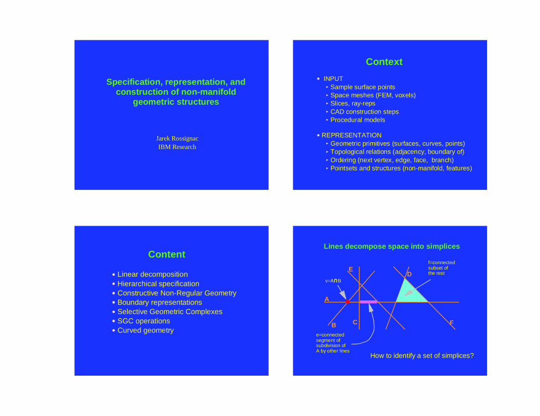
Specification, representation, and construction of non-manifold

geometric structures

Jarek RossignacIBM Research

Context

INPUTSample surface pointsSpace meshes (FEM, voxels)Slices, ray-repsCAD construction stepsProcedural models

REPRESENTATIONGeometric primitives (surfaces, curves, points)Topological relations (adjacency, boundary of)Ordering (next vertex, edge, face, branch)Pointsets and structures (non-manifold, features)

Content

Linear decompositionHierarchical specificationConstructive Non-Regular GeometryBoundary representationsSelective Geometric ComplexesSGC operationsCurved geometry

Lines decompose space into simplices

A

B C

Dv=A B

E

F

e=connected segment of subdivision of A by other lines

f=connectedsubset of the rest

How to identify a set of simplices?

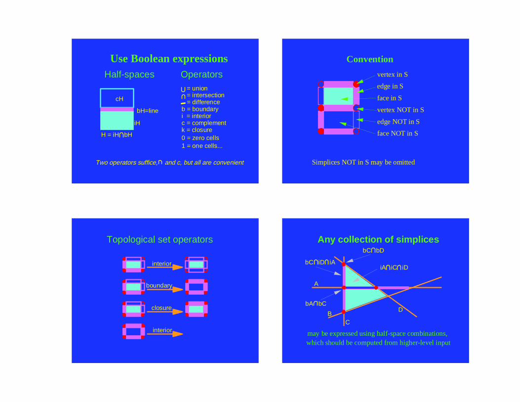
Half-spaces Operators

cH

bH=line

iH

H = iH bH

= union = intersection = differenceb = boundaryi = interiorc = complementk = closure0 = zero cells1 = one cells...

Two operators suffice, and c, but all are convenient

Use Boolean expressions Convention

vertex in S

edge in S

face in S

vertex NOT in S

edge NOT in S

face NOT in S

Simplices NOT in S may be omitted

Topological set operators

interior

boundary

closure

interior

bC bD

A

BC

bC iD iA

D

Any collection of simplices

bA bC

iA iC iD

may be expressed using half-space combinations,which should be computed from higher-level input

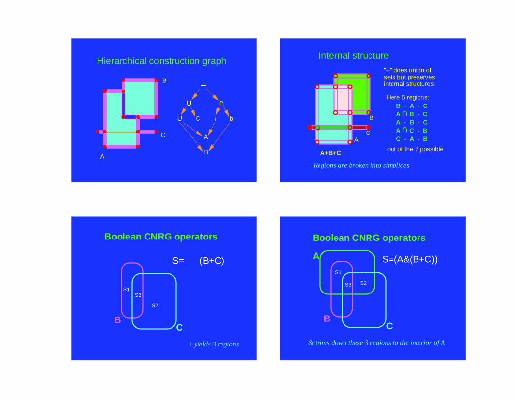
Hierarchical construction graph

A

C

B

A

B

C bi

Internal structure

AC

B

A+B+C

"+" does union ofsets but preservesinternal structures

Here 5 regions:B - A - CA B - CA - B - CA C - BC - A - B

out of the 7 possible

Regions are broken into simplices

Boolean CNRG operators

BC

S= (B+C)

S1

S2

S3

+ yields 3 regions

Boolean CNRG operators

A

BC

S=(A&(B+C))S1

S2S3

& trims down these 3 regions to the interior of A

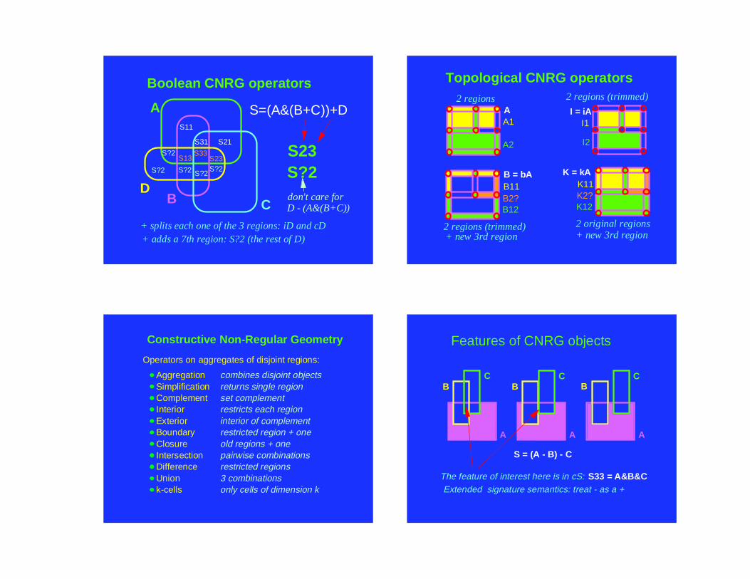
Boolean CNRG operators

A

BD

C

S=(A&(B+C))+DS11

S21S31

S?2S13

S33S23

S?2 S?2 S?2S?2

+ splits each one of the 3 regions: iD and cD+ adds a 7th region: S?2 (the rest of D)

S23S?2

D - (A&(B+C))don't care for

A I = iA

B = bA K = kA

Topological CNRG operators

A1

B11

I1

K11

A2 I2

B12 K12B2? K2?

2 regions 2 regions (trimmed)

2 regions (trimmed)+ new 3rd region

2 original regions+ new 3rd region

Constructive Non-Regular Geometry

AggregationSimplificationComplementInteriorExteriorBoundaryClosureIntersectionDifferenceUnionk-cells

Operators on aggregates of disjoint regions:

combines disjoint objectsreturns single regionset complementrestricts each region interior of complementrestricted region + oneold regions + onepairwise combinationsrestricted regions3 combinationsonly cells of dimension k

Features of CNRG objects

A A A

B B BC C C

S = (A - B) - C

S33 = A&B&CExtended signature semantics: treat - as a +

The feature of interest here is in cS:

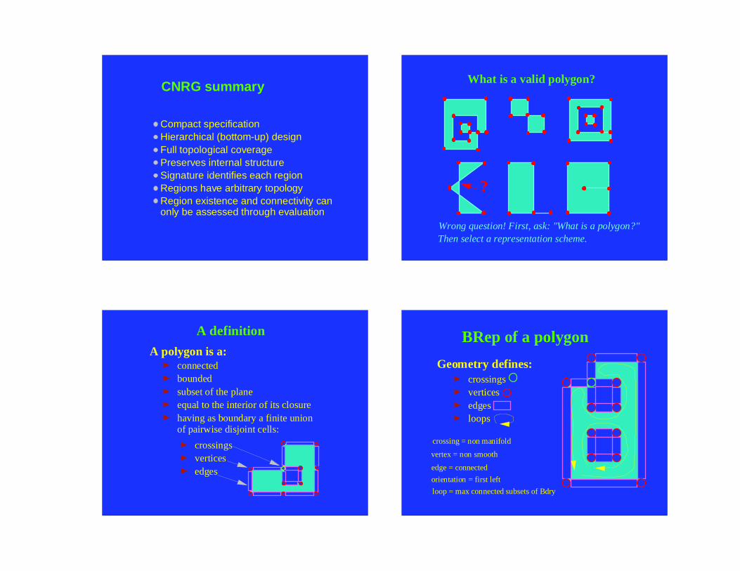
CNRG summary

Compact specificationHierarchical (bottom-up) designFull topological coveragePreserves internal structureSignature identifies each regionRegions have arbitrary topologyRegion existence and connectivity can only be assessed through evaluation

What is a valid polygon?

Wrong question! First, ask: "What is a polygon?"Then select a representation scheme.

?

A definition

connectedboundedsubset of the planeequal to the interior of its closurehaving as boundary a finite unionof pairwise disjoint cells:

crossingsverticesedges

A polygon is a:BRep of a polygon

loop = max connected subsets of Bdry

Geometry defines:crossingsverticesedgesloops

orientation = first left

crossing = non manifold

vertex = non smooth

edge = connected

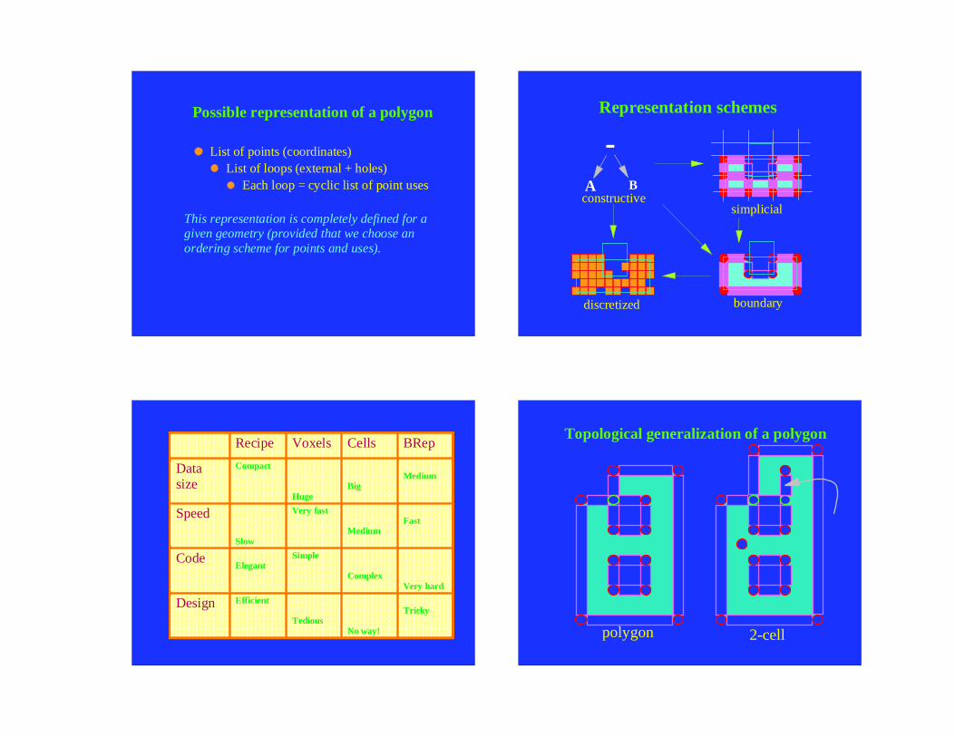
Possible representation of a polygon

List of points (coordinates)List of loops (external + holes)

Each loop = cyclic list of point uses

This representation is completely defined for a given geometry (provided that we choose an ordering scheme for points and uses).

Representation schemes

constructivesimplicial

discretized boundary

A B

-

AAAA

AAAA

AAAA

AAAA

AAAA

AAAA

AAAA

AAAA

AAAA

AAAA

AAAA

AAAA

AAAA

AAAA

AAAA

AAAA

AAAA

AAAA

AAAA

AAAA

AAAA

AAAA

AAAA

AAAA

AAAA

AAAA

AAAA

AAAA

AAAA

AAAA

AAAA

AAAA

AAAA

AAAA

AAAA

AAAA

AAAA

AAAA

AAAA

AAAA

AAAA

AAAA

AAAA

AAAA

AAAA

AAAAAAAA

AAAA

AAAA

AAAA

AAAA

AAAA

AAAA

AAAA

AAAA

AAAA

AAAA

AAAA

AAAA

AAAA

AAAA

AAAA

AAAA

AAAA

AAAA

AAAA

AAAA

AAAA

AAAA

AAAA

AAAA

AAAA

AAAA

AAAA

AAAA

AAAA

AAAA

AAAA

AAAA

AAAA

AAAA

AAAA

AAAA

AAAA

AAAA

AAAA

AAAA

AAAA

AAAA

AAAA

AAAA

AAAAAAAA

AAAA

AAAA

AAAA

AAAA

AAAA

AAAA

AAAA

AAAA

AAAA

AAAA

AAAA

AAAA

AAAA

AAAA

AAAA

AAAA

AAAA

AAAA

AAAA

AAAA

AAAA

AAAA

AAAA

AAAA

AAAA

AAAA

AAAA

AAAA

AAAA

AAAA

AAAA

AAAA

AAAA

AAAA

AAAA

AAAA

AAAA

AAAA

AAAA

AAAA

AAAA

AAAA

AAAA

AAAA

AAAAAAAA

AAAA

AAAA

AAAA

AAAA

AAAA

AAAA

AAAA

AAAA

AAAA

AAAA

AAAA

AAAA

AAAA

AAAA

AAAA

AAAA

AAAA

AAAA

AAAA

AAAA

AAAA

AAAA

AAAA

AAAA

AAAA

AAAA

AAAA

AAAA

AAAA

AAAA

AAAA

AAAA

AAAA

AAAA

AAAA

AAAA

AAAA

AAAA

AAAA

AAAA

AAAA

AAAA

AAAA

AAAA

AAAAAAAA

AAAA

AAAA

AAAA

AAAA

AAAA

AAAA

AAAA

AAAA

AAAA

AAAA

AAAA

AAAA

AAAA

AAAA

AAAA

AAAA

AAAA

AAAA

AAAA

AAAA

AAAA

AAAA

AAAA

AAAA

AAAA

AAAA

AAAA

AAAA

AAAA

AAAA

AAAA

AAAA

AAAA

AAAA

AAAA

AAAA

AAAA

AAAA

AAAA

AAAA

AAAA

AAAA

AAAA

AAAA

AAAAAAAA

AAAA

AAAA

AAAA

AAAA

AAAA

AAAA

AAAA

AAAA

AAAA

AAAA

AAAA

AAAA

AAAA

AAAA

AAAA

AAAA

AAAA

AAAA

AAAA

AAAA

AAAA

AAAA

AAAA

AAAA

AAAA

AAAA

AAAA

AAAA

AAAA

AAAA

AAAA

AAAA

AAAA

AAAA

AAAA

AAAA

AAAA

AAAA

AAAA

AAAA

AAAA

AAAA

AAAA

AAAA

AAAAAAAA

AAAA

AAAA

AAAA

AAAA

AAAA

AAAA

AAAA

AAAA

AAAA

AAAA

AAAA

AAAA

AAAA

AAAA

AAAA

AAAA

AAAA

AAAA

AAAA

AAAA

AAAA

AAAA

AAAA

AAAA

AAAA

AAAA

AAAA

AAAA

AAAA

AAAA

AAAA

AAAA

AAAA

AAAA

AAAA

AAAA

AAAA

AAAA

AAAA

AAAA

AAAA

AAAA

AAAA

AAAA

AAAAAAAA

AAAA

AAAA

AAAA

AAAA

AAAA

AAAA

AAAA

AAAA

AAAA

AAAA

AAAA

AAAA

AAAA

AAAA

AAAA

AAAA

AAAA

AAAA

AAAA

AAAA

AAAA

AAAA

AAAA

AAAA

AAAA

AAAA

AAAA

AAAA

AAAA

AAAA

AAAA

AAAA

AAAA

AAAA

AAAA

AAAA

AAAA

AAAA

AAAA

AAAA

AAAA

AAAA

AAAA

AAAA

AAAAAAAA

AAAA

AAAA

AAAA

AAAA

AAAA

AAAA

AAAA

AAAA

AAAA

AAAA

AAAA

AAAA

AAAA

AAAA

AAAA

AAAA

AAAA

AAAA

AAAA

AAAA

AAAA

AAAA

AAAA

AAAA

AAAA

AAAA

AAAA

AAAA

AAAA

AAAA

AAAA

AAAA

AAAA

AAAA

AAAA

AAAA

AAAA

AAAA

AAAA

AAAA

AAAA

AAAA

AAAA

AAAA

AAAAAAAA

AAAA

AAAA

AAAA

AAAA

AAAA

AAAA

AAAA

AAAA

AAAA

AAAA

AAAA

AAAA

AAAA

AAAA

AAAA

AAAA

AAAA

AAAA

AAAA

AAAA

AAAA

AAAA

AAAA

AAAA

AAAA

AAAA

AAAA

AAAA

AAAA

AAAA

AAAA

AAAA

AAAA

AAAA

AAAA

AAAA

AAAA

AAAA

AAAA

AAAA

AAAA

AAAA

AAAA

AAAA

AAAAAAAA

AAAA

AAAA

AAAA

AAAA

AAAA

AAAA

AAAA

AAAA

AAAA

AAAA

AAAA

AAAA

AAAA

AAAA

AAAA

AAAA

AAAA

AAAA

AAAA

AAAA

AAAA

AAAA

AAAA

AAAA

AAAA

AAAA

AAAA

AAAA

AAAA

AAAA

AAAA

AAAA

AAAA

AAAA

AAAA

AAAA

AAAA

AAAA

AAAA

AAAA

AAAA

AAAA

AAAA

AAAA

AAAAAAAA

AAAA

AAAA

AAAA

AAAA

AAAA

AAAA

AAAA

AAAA

AAAA

AAAA

AAAA

AAAA

AAAA

AAAA

AAAA

AAAA

AAAA

AAAA

AAAA

AAAA

AAAA

AAAA

AAAA

AAAA

AAAA

AAAA

AAAA

AAAA

AAAA

AAAA

AAAA

AAAA

AAAA

AAAA

AAAA

AAAA

AAAA

AAAA

AAAA

AAAA

AAAA

AAAA

AAAA

AAAA

AAAAAAAA

AAAA

AAAA

AAAA

AAAA

AAAA

AAAA

AAAA

AAAA

AAAA

AAAA

AAAA

AAAA

AAAA

AAAA

AAAA

AAAA

AAAA

AAAA

AAAA

AAAA

AAAA

AAAA

AAAA

AAAA

AAAA

AAAA

AAAA

AAAA

AAAA

AAAA

AAAA

AAAA

AAAA

AAAA

AAAA

AAAA

AAAA

AAAA

AAAA

AAAA

AAAA

AAAA

AAAA

AAAA

AAAAAAAA

AAAA

AAAA

AAAA

AAAA

AAAA

AAAA

AAAA

AAAA

AAAA

AAAA

AAAA

AAAA

AAAA

AAAA

AAAA

AAAA

AAAA

AAAA

AAAA

AAAA

AAAA

AAAA

AAAA

AAAA

AAAA

AAAA

AAAA

AAAA

AAAA

AAAA

AAAA

AAAA

AAAA

AAAA

AAAA

AAAA

AAAA

AAAA

AAAA

AAAA

AAAA

AAAA

AAAA

AAAA

AAAAAAAA

AAAA

AAAA

AAAA

AAAA

AAAA

AAAA

AAAA

AAAA

AAAA

AAAA

AAAA

AAAA

AAAA

AAAA

AAAA

AAAA

AAAA

AAAA

AAAA

AAAA

AAAA

AAAA

AAAA

AAAA

AAAA

AAAA

AAAA

AAAA

AAAA

AAAA

AAAA

AAAA

AAAA

AAAA

AAAA

AAAA

AAAA

AAAA

AAAA

AAAA

AAAA

AAAA

AAAA

AAAA

AAAAAAA

AAA

AAA

AAA

AAA

AAA

AAA

AAA

AAA

AAA

AAA

AAA

AAA

AAA

AAA

AAA

AAA

AAA

AAA

AAA

AAA

AAA

AAA

AAA

AAA

AAA

AAA

AAA

AAA

AAA

AAA

AAA

AAA

AAA

AAA

AAA

AAA

AAA

AAA

AAA

AAA

AAA

AAA

AAA

AAA

AAA

AAAA

AAAA

AAAA

AAAA

AAAA

AAAA

AAAAAAAA

AAAA

AAAA

AAAA

AAAA

AAAA

AAAAAAAA

AAAA

AAAA

AAAA

AAAA

AAAA

AAAAAAAAAAA

AAAA

AAAA

AAAA

AAAA

AAAA

AAAA

AAAAAAAA

AAAA

AAAA

AAAA

AAAA

AAAA

AAAAAAAA

AAAA

AAAA

AAAA

AAAA

AAAA

AAAAAA

AAAAAAAAAAAA

Recipe

AAAA

AAAA

AAAA

AAAA

AAAA

AAAA

AAAAAAAA

AAAA

AAAA

AAAA

AAAA

AAAA

AAAAAAAA

AAAA

AAAA

AAAA

AAAA

AAAA

AAAA

Voxels

AAAA

AAAA

AAAA

AAAA

AAAA

AAAA

AAAAAAAA

AAAA

AAAA

AAAA

AAAA

AAAA

AAAAAAAA

AAAA

AAAA

AAAA

AAAA

AAAA

AAAA

Cells

AAAA

AAAA

AAAA

AAAA

AAAA

AAAA

AAAAAAAA

AAAA

AAAA

AAAA

AAAA

AAAA

AAAAAAAA

AAAA

AAAA

AAAA

AAAA

AAAA

AAAA

BRep

AAAA

AAAA

AAAA

AAAA

AAAA

AAAA

AAAA

AAAA

AAAA

AAAAAAAA

AAAA

AAAA

AAAA

AAAA

AAAA

AAAA

AAAA

AAAA

AAAAAAAA

AAAA

AAAA

AAAA

AAAA

AAAA

AAAA

AAAA

AAAA

AAAAAAAAAAAAAA

Data size

AAAA

AAAA

AAAA

AAAA

AAAA

AAAA

AAAA

AAAA

AAAA

AAAAAAAA

AAAA

AAAA

AAAA

AAAA

AAAA

AAAA

AAAA

AAAA

AAAAAAAA

AAAA

AAAA

AAAA

AAAA

AAAA

AAAA

AAAA

AAAA

AAAAAAAAAAAAAAAAAAAAAAAA

Compact

AAAA

AAAA

AAAA

AAAA

AAAA

AAAA

AAAA

AAAA

AAAA

AAAAAAAA

AAAA

AAAA

AAAA

AAAA

AAAA

AAAA

AAAA

AAAA

AAAAAAAA

AAAA

AAAA

AAAA

AAAA

AAAA

AAAA

AAAA

AAAA

AAAA

Huge

AAAA

AAAA

AAAA

AAAA

AAAA

AAAA

AAAA

AAAA

AAAA

AAAAAAAA

AAAA

AAAA

AAAA

AAAA

AAAA

AAAA

AAAA

AAAA

AAAAAAAA

AAAA

AAAA

AAAA

AAAA

AAAA

AAAA

AAAA

AAAA

AAAA

Big

AAAA

AAAA

AAAA

AAAA

AAAA

AAAA

AAAA

AAAA

AAAA

AAAAAAAA

AAAA

AAAA

AAAA

AAAA

AAAA

AAAA

AAAA

AAAA

AAAAAAAA

AAAA

AAAA

AAAA

AAAA

AAAA

AAAA

AAAA

AAAA

AAAA

Medium

AAAA

AAAA

AAAA

AAAA

AAAA

AAAA

AAAA

AAAA

AAAA

AAAAAAAA

AAAA

AAAA

AAAA

AAAA

AAAA

AAAA

AAAA

AAAA

AAAAAAAA

AAAA

AAAA

AAAA

AAAA

AAAA

AAAA

AAAA

AAAA

AAAAAAAAAAAAAA

Speed

AAAA

AAAA

AAAA

AAAA

AAAA

AAAA

AAAA

AAAA

AAAA

AAAAAAAA

AAAA

AAAA

AAAA

AAAA

AAAA

AAAA

AAAA

AAAA

AAAAAAAA

AAAA

AAAA

AAAA

AAAA

AAAA

AAAA

AAAA

AAAA

AAAAAAAA

AAAAAAAAAAAAAAAA

Slow

AAAA

AAAA

AAAA

AAAA

AAAA

AAAA

AAAA

AAAA

AAAA

AAAAAAAA

AAAA

AAAA

AAAA

AAAA

AAAA

AAAA

AAAA

AAAA

AAAAAAAA

AAAA

AAAA

AAAA

AAAA

AAAA

AAAA

AAAA

AAAA

AAAA

Very fast

AAAA

AAAA

AAAA

AAAA

AAAA

AAAA

AAAA

AAAA

AAAA

AAAAAAAA

AAAA

AAAA

AAAA

AAAA

AAAA

AAAA

AAAA

AAAA

AAAAAAAA

AAAA

AAAA

AAAA

AAAA

AAAA

AAAA

AAAA

AAAA

AAAA

Medium

AAAA

AAAA

AAAA

AAAA

AAAA

AAAA

AAAA

AAAA

AAAA

AAAAAAAA

AAAA

AAAA

AAAA

AAAA

AAAA

AAAA

AAAA

AAAA

AAAAAAAA

AAAA

AAAA

AAAA

AAAA

AAAA

AAAA

AAAA

AAAA

AAAA

Fast

AAAA

AAAA

AAAA

AAAA

AAAA

AAAA

AAAA

AAAA

AAAA

AAAA

AAAAAAAA

AAAA

AAAA

AAAA

AAAA

AAAA

AAAA

AAAA

AAAA

AAAA

AAAAAAAA

AAAA

AAAA

AAAA

AAAA

AAAA

AAAA

AAAA

AAAA

AAAA

AAAAAAAAAAAAAAA

Code

AAAA

AAAA

AAAA

AAAA

AAAA

AAAA

AAAA

AAAA

AAAA

AAAA

AAAAAAAA

AAAA

AAAA

AAAA

AAAA

AAAA

AAAA

AAAA

AAAA

AAAA

AAAAAAAA

AAAA

AAAA

AAAA

AAAA

AAAA

AAAA

AAAA

AAAA

AAAA

AAAAAAAAAAAA

AAAAAAAAAAAAAA

Elegant

AAAA

AAAA

AAAA

AAAA

AAAA

AAAA

AAAA

AAAA

AAAA

AAAA

AAAAAAAA

AAAA

AAAA

AAAA

AAAA

AAAA

AAAA

AAAA

AAAA

AAAA

AAAAAAAA

AAAA

AAAA

AAAA

AAAA

AAAA

AAAA

AAAA

AAAA

AAAA

AAAA

Simple

AAAA

AAAA

AAAA

AAAA

AAAA

AAAA

AAAA

AAAA

AAAA

AAAA

AAAAAAAA

AAAA

AAAA

AAAA

AAAA

AAAA

AAAA

AAAA

AAAA

AAAA

AAAAAAAA

AAAA

AAAA

AAAA

AAAA

AAAA

AAAA

AAAA

AAAA

AAAA

AAAA

Complex

AAAA

AAAA

AAAA

AAAA

AAAA

AAAA

AAAA

AAAA

AAAA

AAAA

AAAAAAAA

AAAA

AAAA

AAAA

AAAA

AAAA

AAAA

AAAA

AAAA

AAAA

AAAAAAAA

AAAA

AAAA

AAAA

AAAA

AAAA

AAAA

AAAA

AAAA

AAAA

AAAA

Very hard

AAAA

AAAA

AAAA

AAAA

AAAA

AAAA

AAAA

AAAA

AAAA

AAAAAAAA

AAAA

AAAA

AAAA

AAAA

AAAA

AAAA

AAAA

AAAA

AAAAAAAA

AAAA

AAAA

AAAA

AAAA

AAAA

AAAA

AAAA

AAAA

AAAAA

AA

AAAAAAA

Design

AAAA

AAAA

AAAA

AAAA

AAAA

AAAA

AAAA

AAAA

AAAA

AAAAAAAA

AAAA

AAAA

AAAA

AAAA

AAAA

AAAA

AAAA

AAAA

AAAAAAAA

AAAA

AAAA

AAAA

AAAA

AAAA

AAAA

AAAA

AAAA

AAAAAAAA

AAAA

AAAAAAAAAAAA

Efficient

AAAA

AAAA

AAAA

AAAA

AAAA

AAAA

AAAA

AAAA

AAAA

AAAAAAAA

AAAA

AAAA

AAAA

AAAA

AAAA

AAAA

AAAA

AAAA

AAAAAAAA

AAAA

AAAA

AAAA

AAAA

AAAA

AAAA

AAAA

AAAA

AAAATedious

AAAA

AAAA

AAAA

AAAA

AAAA

AAAA

AAAA

AAAA

AAAA

AAAAAAAA

AAAA

AAAA

AAAA

AAAA

AAAA

AAAA

AAAA

AAAA

AAAAAAAA

AAAA

AAAA

AAAA

AAAA

AAAA

AAAA

AAAA

AAAA

AAAA

No way!

AAAA

AAAA

AAAA

AAAA

AAAA

AAAA

AAAA

AAAA

AAAA

AAAAAAAA

AAAA

AAAA

AAAA

AAAA

AAAA

AAAA

AAAA

AAAA

AAAAAAAA

AAAA

AAAA

AAAA

AAAA

AAAA

AAAA

AAAA

AAAA

AAAA

Tricky

polygon 2-cell

Topological generalization of a polygon

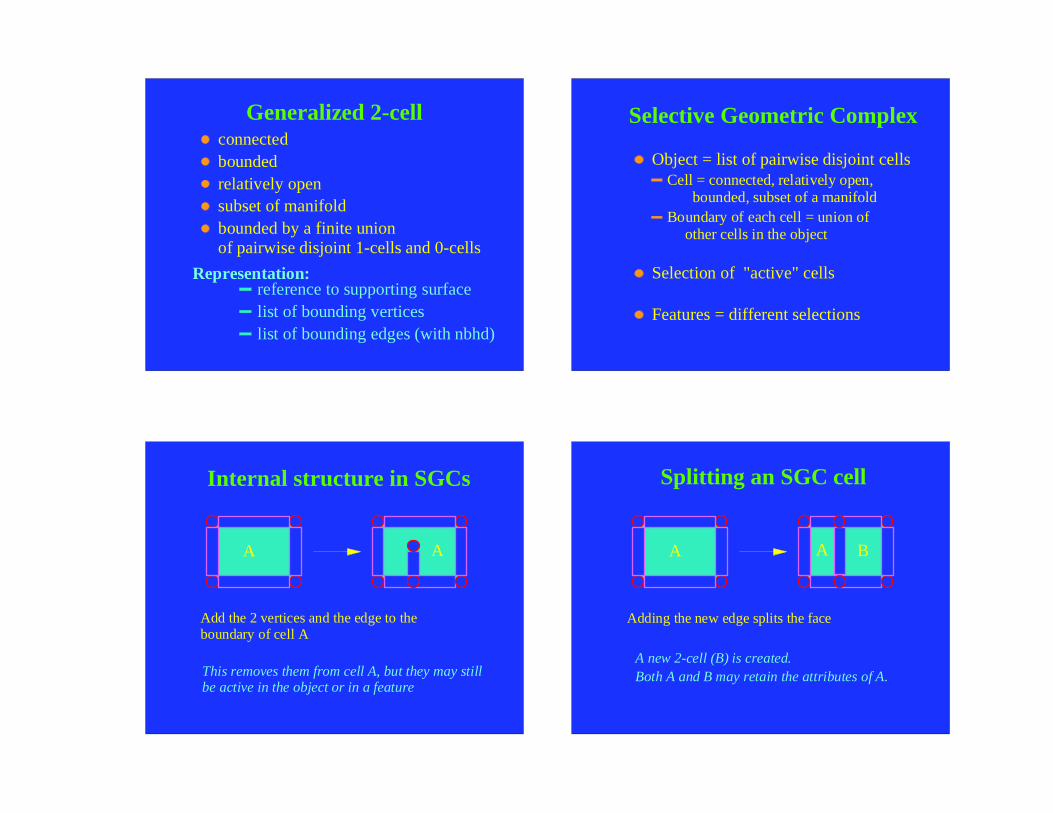
Generalized 2-cellconnectedboundedrelatively opensubset of manifoldbounded by a finite union of pairwise disjoint 1-cells and 0-cells

reference to supporting surfacelist of bounding verticeslist of bounding edges (with nbhd)

Representation:

Selective Geometric Complex

Object = list of pairwise disjoint cellsCell = connected, relatively open,

bounded, subset of a manifoldBoundary of each cell = union of

other cells in the object

Selection of "active" cells

Features = different selections

Internal structure in SGCs

Add the 2 vertices and the edge to the boundary of cell A

A

This removes them from cell A, but they may still be active in the object or in a feature

A

Splitting an SGC cell

Adding the new edge splits the face

A

A new 2-cell (B) is created. Both A and B may retain the attributes of A.

BA

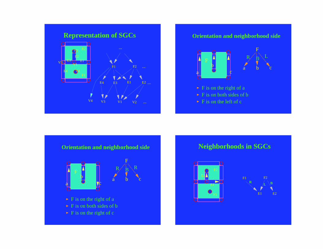
Representation of SGCs

F2F1

E1 E2

V1 V2

F2

F1

E1E2

V1

V2

E3

E4

E3E4

V3

V3 ...

...

...

...

V4

V4

Orientation and neighborhood side

ab

c

F

F is on the right of aF is on both sides of bF is on the left of c

F

a b c

R B L

Orientation and neighborhood side

ab

c

F

F is on the right of aF is on both sides of bF is on the right of c

F

a b c

R B R

Neighborhoods in SGCs

F2F1

E1 E2

F2

F1

E1

E2

BLR

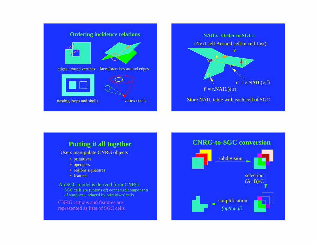
Ordering incidence relations

edges around verticesfaces/branches around edges

nesting loops and shells vertex cones

12

34

NAILs: Order in SGCs

efv

e' = e.NAIL(v,f)

e'

f'

f' = f.NAIL(e,r)

r(Next cell Around cell In cell List)

Store NAIL table with each cell of SGC

Putting it all togetherUsers manipulate CNRG objects

primitivesoperatorsregions signaturesfeatures

CNRG regions and features are represented as lists of SGC cells

An SGC model is derived from CNRGSGC cells are (unions of) connected components of simplices induced by primitives' cells

CNRG-to-SGC conversion

subdivision

selection(A+B)-C

simplification

(optional)

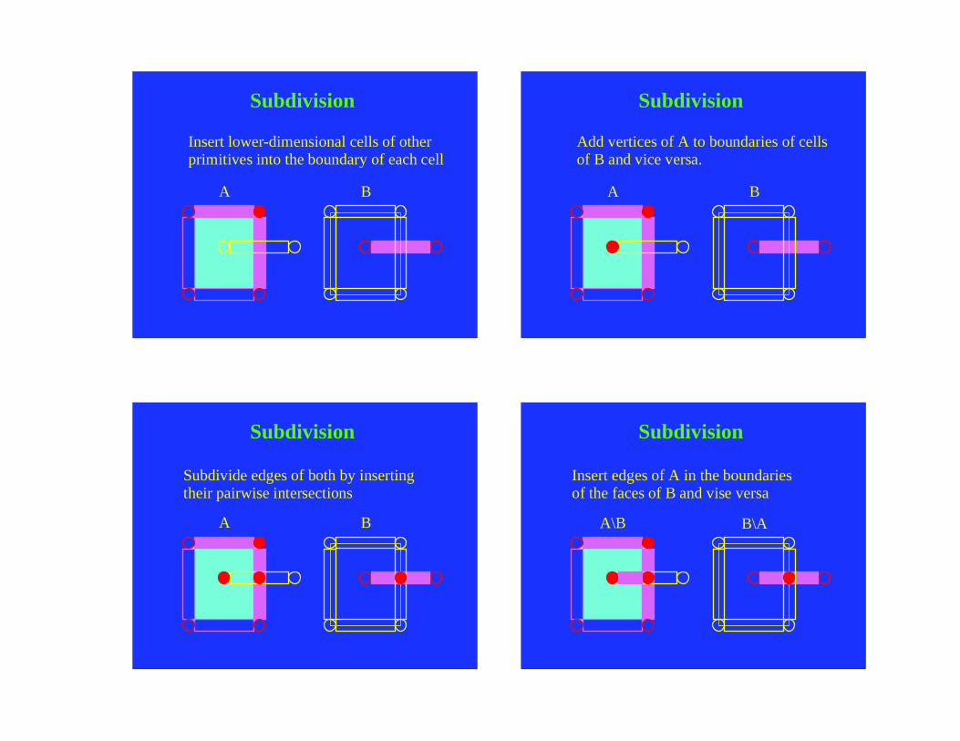
Subdivision

Insert lower-dimensional cells of otherprimitives into the boundary of each cell

A B

Subdivision

Add vertices of A to boundaries of cells of B and vice versa.

A B

Subdivision

Subdivide edges of both by insertingtheir pairwise intersections

A B

Subdivision

Insert edges of A in the boundaries of the faces of B and vise versa

A\B B\A

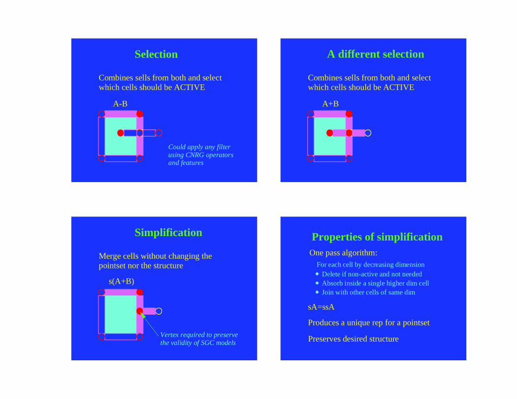
Selection

Combines sells from both and selectwhich cells should be ACTIVE

A-B

Could apply any filter using CNRG operators and features

A different selection

Combines sells from both and selectwhich cells should be ACTIVE

A+B

Simplification

Merge cells without changing thepointset nor the structure

s(A+B)

Vertex required to preservethe validity of SGC models

Properties of simplification

sA=ssA

Produces a unique rep for a pointset

One pass algorithm:For each cell by decreasing dimension

Delete if non-active and not neededAbsorb inside a single higher dim cellJoin with other cells of same dim

Preserves desired structure

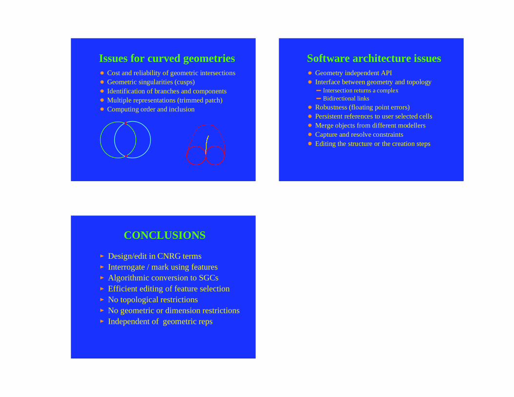
Issues for curved geometriesCost and reliability of geometric intersectionsGeometric singularities (cusps)Identification of branches and componentsMultiple representations (trimmed patch)Computing order and inclusion

Software architecture issuesGeometry independent APIInterface between geometry and topology

Intersection returns a complexBidirectional links

Robustness (floating point errors)Persistent references to user selected cellsMerge objects from different modellersCapture and resolve constraintsEditing the structure or the creation steps

CONCLUSIONS

Design/edit in CNRG termsInterrogate / mark using featuresAlgorithmic conversion to SGCsEfficient editing of feature selectionNo topological restrictions No geometric or dimension restrictionsIndependent of geometric reps

Modeling with Simplicial Complexes

(Topology, Geometry, and Algorithms)1

Herbert Edelsbrunner2

Abstract. Geometric modeling often refers to forming and deforming geometric shape. This paper considers

the use of simplicial complexes as a general representation of shapes supporting algorithmic solutions to a variety

of geometric modeling problems. At this moment, rather little of the potential of simplicial complexes has been

exploited algorithmically, and we concentrate on mathematical results that seem most promising to lead to novel

algorithmic methods and ideas.

Keywords. Solid modeling, computational geometry, combinatorial topology, grid generation; simplicial complexes, nerves,

Voronoi cells, Delaunay simplicial complexes.

1This work is partially supported by the National Science Foundation, under grant ASC-9200301 and the Alan T. Waterman award,

grant CCR-9118874. Any opinions, ndings, conclusions, or recommendations expressed in this publication are those of the authors

and do not necessarily re ect the view of the National Science Foundation.2Department of Computer Science, University of Illinois at Urbana-Champaign, Urbana, Illinois 61801, USA.

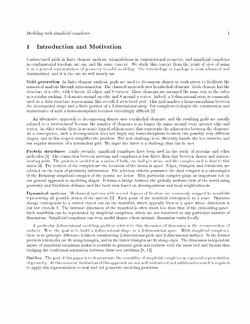
Modeling with simplicial complexes 1

1 Introduction and Motivation

Unstructured grids in nite element analysis, triangulations in computational geometry, and simplicial complexes

in combinatorial topology are one and the same concept. We study this concept from the point of view of using

it as a general representation of geometry in solid modeling. The terminology in topology is most advanced and

standardized, and it is the one we will mostly use.

Grid generation. In nite element analysis, grids are used to decompose shapes or work-pieces to facilitate the

numerical analysis through approximation. The classical approach uses hexahedral elements. Each element has the

structure of a cube, with 6 facets, 12 edges, and 8 vertices. These elements are arranged the same way as the cubes

in a regular packing, 4 elements around an edge and 8 around a vertex. Indeed, a 3-dimensional array is commonly

used as a data structure representing this so-called structured grid. This grid implies a homeomorphism between

the decomposed shape and a nite portion of a 3-dimensional array. For complicated shapes the construction and

maintenance of such a homeomorphism becomes exceedingly dicult [2].

An alternative approach to decomposing shapes uses tetrahedral elements, and the resulting grids are usually

referred to a unstructured because the number of elements is no longer the same around every interior edge and

vertex. In other words, there is no static logical address space that represents the adjacencies between the elements.

As a consequence, such a decomposition does not imply any homeomorphism between two possibly very dierent

shapes, and in this respect simplies the problem. The new challenge is to eciently handle the less intuitive and

less regular structure of a tetrahedral grid. We argue the latter is a challenge that can be met.

Protein structures. Fairly recently, simplicial complexes have been used in the study of proteins and other

molecules [5]. The connection between proteins and complexes is less direct than that between shapes and approx-

imating grids. The protein is modeled as a union of balls, one ball per atom, and the complex used is dual to this

union [4]. The vertices of the complex are the locations of the atoms in space. Edges, triangles, and tetrahedra are

selected on the basis of proximity information. The selection criteria guarantee the dual complex is a subcomplex

of the Delaunay simplicial complex of the points, see below. This particular complex plays an important role in

our general approach to modeling shapes. It forms a bridge between the globally uniform view of the world using

geometry and Euclidean distance and the local view based on decompositions and local neighborhoods.

Dynamical systems. Mechanical systems with several degrees of freedom are commonly mapped to manifolds

representing all possible states of the system [1]. Each point of the manifold corresponds to a state. Dynamic

change corresponds to a curved traced out on the manifold, which typically lives in a space whose dimension is

low but exceeds 3. The intrinsic dimension of the manifold is often much less than that of the embedding space.

Such manifolds can be represented by simplicial complexes, which are not restricted to any particular number of

dimensions. Simplicial complexes can even model shapes whose intrinsic dimension varies locally.

A particular 3-dimensional modeling problem related to this discussion of dimension is the reconstruction of

surfaces. Here the goal is to build a 2-dimensional shape in a 3-dimensional space. With simplicial complexes,

there is no principle dierence between constructing 3-dimensional grids and 2-dimensional surfaces. In the former

problem tetrahedra are t along triangles, and in the latter triangles are t along edges. The dimension independent

aspect of simplicial complexes makes it possible to generate grids and surfaces with the same tool and format thus

bridging the traditional separation between these two problems [8, 14].

Outline. The goal of this paper is to demonstrate the versatility of simplicial complexes as a general representation

of geometry. At this moment, limitations of this approach are not well understood and additional research is required

to apply this representation to new and old geometric modeling problems.

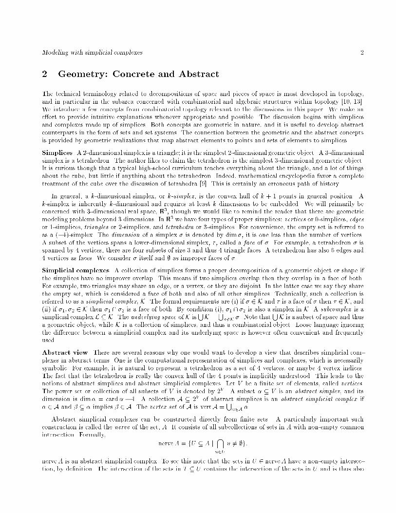
Modeling with simplicial complexes 2

2 Geometry: Concrete and Abstract

The technical terminology related to decompositions of space and pieces of space is most developed in topology,

and in particular in the subarea concerned with combinatorial and algebraic structures within topology [10, 13].

We introduce a few concepts from combinatorial topology relevant to the discussions in this paper. We make an

eort to provide intuitive explanations whenever appropriate and possible. The discussion begins with simplices

and complexes made up of simplices. Both concepts are geometric in nature, and it is useful to develop abstract

counterparts in the form of sets and set systems. The connection between the geometric and the abstract concepts

is provided by geometric realizations that map abstract elements to points and sets of elements to simplices.

Simplices. A 2-dimensional simplex is a triangle; it is the simplest 2-dimensional geometric object. A 3-dimensional

simplex is a tetrahedron. The author likes to claim the tetrahedron is the simplest 3-dimensional geometric object.

It is curious though that a typical high-school curriculum teaches everything about the triangle, and a lot of things

about the cube, but little if anything about the tetrahedron. Indeed, mathematical encyclopedia favor a complete

treatment of the cube over the discussion of tetrahedra [9]. This is certainly an erroneous path of history.

In general, a k-dimensional simplex, or k-simplex, is the convex hull of k + 1 points in general position. A

k-simplex is inherently k-dimensional and requires at least k dimensions to be embedded. We will primarily be

concerned with 3-dimensional real space, R3, though we would like to remind the reader that there are geometric

modeling problems beyond 3 dimensions. In R3 we have four types of proper simplices: vertices or 0-simplices, edges

or 1-simplices, triangles or 2-simplices, and tetrahedra or 3-simplices. For convenience, the empty set is referred to

as a (1)-simplex. The dimension of a simplex is denoted by dim; it is one less than the number of vertices.

A subset of the vertices spans a lower-dimensional simplex, , called a face of . For example, a tetrahedron is

spanned by 4 vertices, there are four subsets of size 3 and thus 4 triangle faces. A tetrahedron has also 6 edges and

4 vertices as faces. We consider itself and ; as improper faces of .

Simplicial complexes. A collection of simplices forms a proper decomposition of a geometric object or shape if

the simplices have no improver overlap. This means if two simplices overlap then they overlap in a face of both.

For example, two triangles may share an edge, or a vertex, or they are disjoint. In the latter case we say they share

the empty set, which is considered a face of both and also of all other simplices. Technically, such a collection is

referred to as a simplicial complex, K. The formal requirements are (i) if 2 K and is a face of then 2 K, and

(ii) if 1; 2 2 K then 1 \ 2 is a face of both. By condition (i), 1 \ 2 is also a simplex in K. A subcomplex is a

simplicial complex L K. The underlying space of K isSK =S2K . Note that

SK is a subset of space and thus

a geometric object, while K is a collection of simplices, and thus a combinatorial object. Loose language ignoring

the dierence between a simplicial complex and its underlying space is however often convenient and frequently

used.

Abstract view. There are several reasons why one would want to develop a view that describes simplicial com-

plexes in abstract terms. One is the computational representation of simplices and complexes, which is necessarily

symbolic. For example, it is natural to represent a tetrahedron as a set of 4 vertices, or maybe 4 vertex indices.

The fact that the tetrahedron is really the convex hull of the 4 points is implicitly understood. This leads to the

notions of abstract simplices and abstract simplicial complexes. Let V be a nite set of elements, called vertices.

The power set or collection of all subsets of V is denoted by 2V . A subset V is an abstract simplex, and its

dimension is dim = card 1. A collection A 2V of abstract simplices is an abstract simplicial complex if

2 A and implies 2 A. The vertex set of A is vertA =S2A .

Abstract simplicial complexes can be constructed directly from nite sets. A particularly important such

construction is called the nerve of the set, A. It consists of all subcollections of sets in A with non-empty common

intersection. Formally,

nerveA = fU A j

\

u2U

u 6= ;g:

nerveA is an abstract simplicial complex. To see this note that the sets in U 2 nerveA have a non-empty intersec-

tion, by denition. The intersection of the sets in T U contains the intersection of the sets in U and is thus also

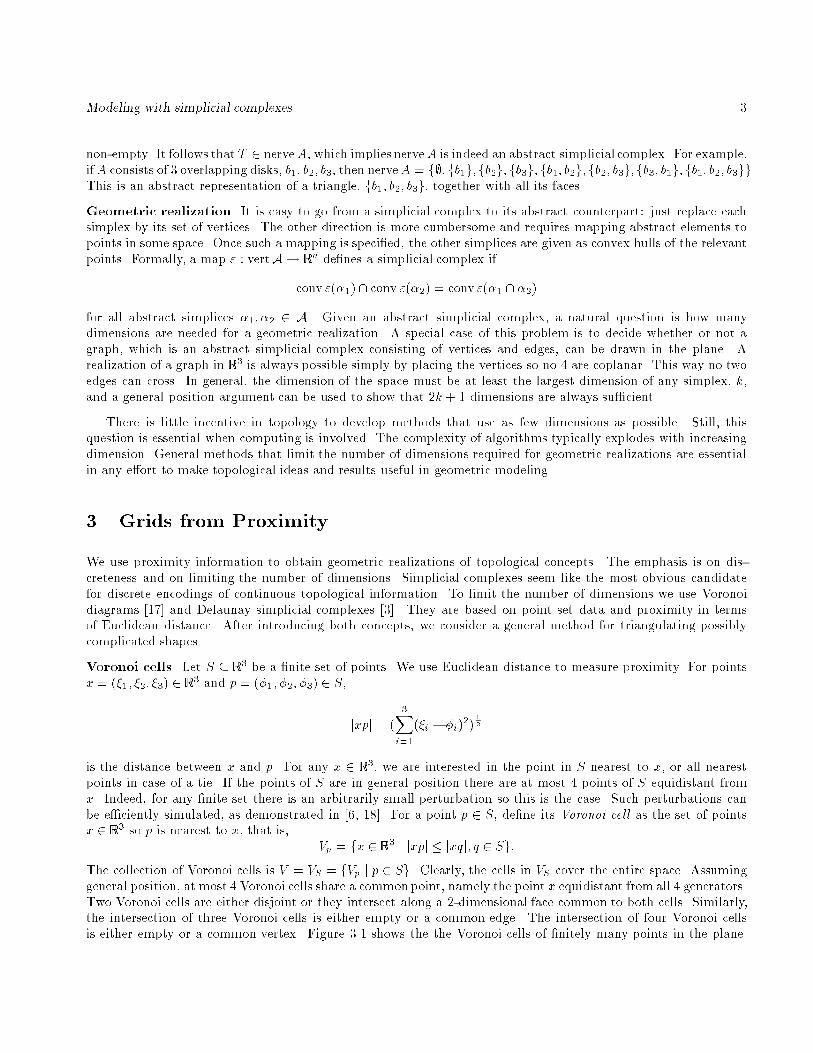
Modeling with simplicial complexes 3

non-empty. It follows that T 2 nerveA, which implies nerveA is indeed an abstract simplicial complex. For example,

ifA consists of 3 overlapping disks, b1; b2; b3, then nerveA = f;; fb1g; fb2g; fb3g; fb1; b2g; fb2; b3g; fb3; b1g; fb1; b2; b3gg.

This is an abstract representation of a triangle, fb1; b2; b3g, together with all its faces.

Geometric realization. It is easy to go from a simplicial complex to its abstract counterpart: just replace each

simplex by its set of vertices. The other direction is more cumbersome and requires mapping abstract elements to

points in some space. Once such a mapping is specied, the other simplices are given as convex hulls of the relevant

points. Formally, a map " : vertA ! Rd denes a simplicial complex if

conv "(1) \ conv "(2) = conv "(1 \ 2)

for all abstract simplices 1; 2 2 A. Given an abstract simplicial complex, a natural question is how many

dimensions are needed for a geometric realization. A special case of this problem is to decide whether or not a

graph, which is an abstract simplicial complex consisting of vertices and edges, can be drawn in the plane. A

realization of a graph in R3 is always possible simply by placing the vertices so no 4 are coplanar. This way no two

edges can cross. In general, the dimension of the space must be at least the largest dimension of any simplex, k,

and a general position argument can be used to show that 2k + 1 dimensions are always sucient.

There is little incentive in topology to develop methods that use as few dimensions as possible. Still, this

question is essential when computing is involved. The complexity of algorithms typically explodes with increasing

dimension. General methods that limit the number of dimensions required for geometric realizations are essential

in any eort to make topological ideas and results useful in geometric modeling.

3 Grids from Proximity

We use proximity information to obtain geometric realizations of topological concepts. The emphasis is on dis-

creteness and on limiting the number of dimensions. Simplicial complexes seem like the most obvious candidate

for discrete encodings of continuous topological information. To limit the number of dimensions we use Voronoi

diagrams [17] and Delaunay simplicial complexes [3]. They are based on point set data and proximity in terms

of Euclidean distance. After introducing both concepts, we consider a general method for triangulating possibly

complicated shapes.

Voronoi cells. Let S R3 be a nite set of points. We use Euclidean distance to measure proximity. For points

x = (1; 2; 3) 2 R3 and p = (1; 2; 3) 2 S,

jxpj = (

3X

i=1

(i i)2)

1

2

is the distance between x and p. For any x 2 R3, we are interested in the point in S nearest to x, or all nearest

points in case of a tie. If the points of S are in general position there are at most 4 points of S equidistant from

x. Indeed, for any nite set there is an arbitrarily small perturbation so this is the case. Such perturbations can

be eciently simulated, as demonstrated in [6, 18]. For a point p 2 S, dene its Voronoi cell as the set of points

x 2 R3 so p is nearest to x, that is,

Vp = fx 2 R3 j jxpj jxqj; q 2 Sg:

The collection of Voronoi cells is V = VS = fVp j p 2 Sg. Clearly, the cells in VS cover the entire space. Assuming

general position, at most 4 Voronoi cells share a commonpoint, namely the point x equidistant from all 4 generators.

Two Voronoi cells are either disjoint or they intersect along a 2-dimensional face common to both cells. Similarly,

the intersection of three Voronoi cells is either empty or a common edge. The intersection of four Voronoi cells

is either empty or a common vertex. Figure 3.1 shows the the Voronoi cells of nitely many points in the plane.

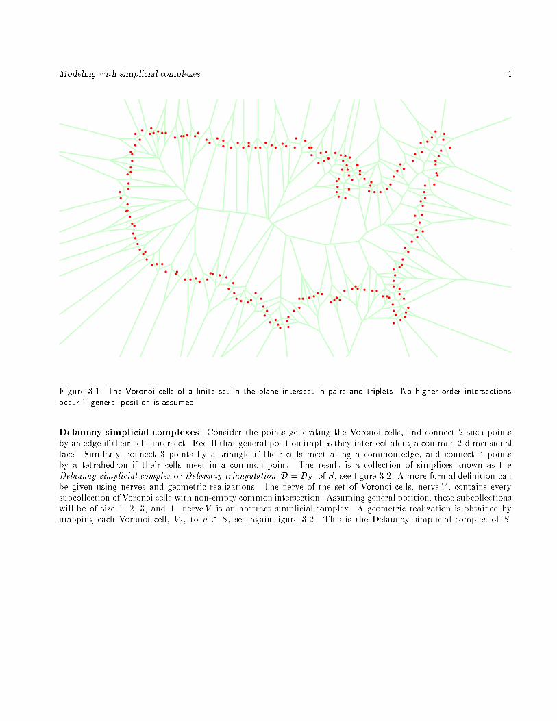
Modeling with simplicial complexes 4

Figure 3.1: The Voronoi cells of a nite set in the plane intersect in pairs and triplets. No higher order intersectionsoccur if general position is assumed.

Delaunay simplicial complexes. Consider the points generating the Voronoi cells, and connect 2 such points

by an edge if their cells intersect. Recall that general position implies they intersect along a common 2-dimensional

face. Similarly, connect 3 points by a triangle if their cells meet along a common edge, and connect 4 points

by a tetrahedron if their cells meet in a common point. The result is a collection of simplices known as the

Delaunay simplicial complex or Delaunay triangulation, D = DS , of S, see gure 3.2. A more formal denition can

be given using nerves and geometric realizations. The nerve of the set of Voronoi cells, nerve V , contains every

subcollection of Voronoi cells with non-empty common intersection. Assuming general position, these subcollections

will be of size 1, 2, 3, and 4. nerve V is an abstract simplicial complex. A geometric realization is obtained by

mapping each Voronoi cell, Vp, to p 2 S, see again gure 3.2. This is the Delaunay simplicial complex of S.

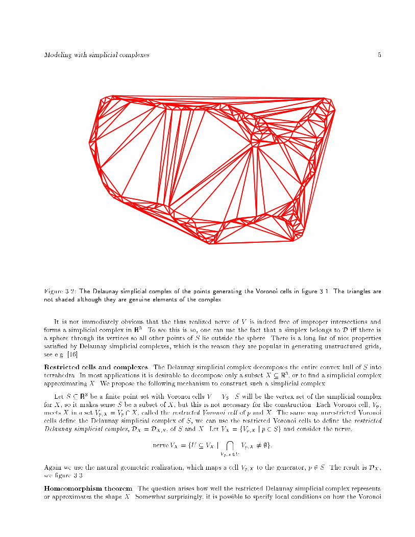
Modeling with simplicial complexes 5

Figure 3.2: The Delaunay simplicial complex of the points generating the Voronoi cells in gure 3.1. The triangles arenot shaded although they are genuine elements of the complex.

It is not immediately obvious that the thus realized nerve of V is indeed free of improper intersections and

forms a simplicial complex in R3. To see this is so, one can use the fact that a simplex belongs to D i there is

a sphere through its vertices so all other points of S lie outside the sphere. There is a long list of nice properties

satised by Delaunay simplicial complexes, which is the reason they are popular in generating unstructured grids,

see e.g. [16].

Restricted cells and complexes. The Delaunay simplicial complex decomposes the entire convex hull of S into

tetrahedra. In most applications it is desirable to decompose only a subset X R3, or to nd a simplicial complex

approximating X. We propose the following mechanism to construct such a simplicial complex.

Let S R3 be a nite point set with Voronoi cells V = VS . S will be the vertex set of the simplicial complex

for X, so it makes sense S be a subset of X, but this is not necessary for the construction. Each Voronoi cell, Vp,

meets X in a set Vp;X = Vp \X, called the restricted Voronoi cell of p and X. The same way unrestricted Voronoi

cells dene the Delaunay simplicial complex of S, we can use the restricted Voronoi cells to dene the restricted

Delaunay simplicial complex, DX = DX;S , of S and X. Let VX = fVp;X j p 2 Sg and consider the nerve,

nerve VX = fU VX j

\

Vp;X2U

Vp;X 6= ;g:

Again we use the natural geometric realization, which maps a cell Vp;X to the generator, p 2 S. The result is DX ,

see gure 3.3.

Homeomorphism theorem. The question arises how well the restricted Delaunay simplicial complex represents

or approximates the shape X. Somewhat surprisingly, it is possible to specify local conditions on how the Voronoi

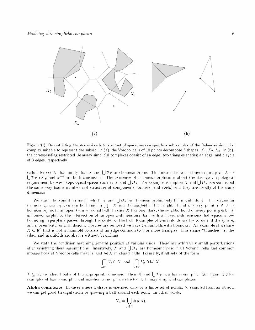
Modeling with simplicial complexes 6

(a) (b)

X1

X3

X2

Figure 3.3: By restricting the Voronoi cells to a subset of space, we can specify a subcomplex of the Delaunay simplicialcomplex suitable to represent the subset. In (a), the Voronoi cells of 10 points decompose 3 shapes, X1; X2; X3. In (b),the corresponding restricted Delaunay simplicial complexes consist of an edge, two triangles sharing an edge, and a cycleof 3 edges, respectively.

cells intersect X that imply that X andSDX are homeomorphic. This means there is a bijective map ' : X !S

DX so ' and '1 are both continuous. The existence of a homeomorphism is about the strongest topological

requirement between topological spaces such as X andSDX . For example, it implies X and

SDX are connected

the same way (same number and structure of components, tunnels, and voids) and they are locally of the same

dimension.

We state the condition under which X andSDX are homeomorphic only for manifolds X. The extension

to more general spaces can be found in [7]. X is a k-manifold if the neighborhood of every point x 2 X is

homeomorphic to an open k-dimensional ball. In case X has boundary, the neighborhood of every point y 2 bdX

is homeomorphic to the intersection of an open k-dimensional ball with a closed k-dimensional half-space whose

bounding hyperplane passes through the center of the ball. Examples of 2-manifolds are the torus and the sphere,

and if open patches with disjoint closures are removed we have 2-manifolds with boundary. An example of a shape

X R3 that is not a manifold consists of an edge common to 3 or more triangles. This shape \branches" at the

edge, and manifolds are shapes without branching.

We state the condition assuming general position of various kinds. There are arbitrarily small perturbations

of S satisfying these assumptions. Intuitively, X andSDX are homeomorphic if all Voronoi cells and common

intersections of Voronoi cells meet X and bdX in closed balls. Formally, if all sets of the form\

p2T

Vp \X and\

p2T

Vp \ bdX;

T S, are closed balls of the appropriate dimension then X andSDX are homeomorphic. See gure 3.3 for

examples of homeomorphic and non-homeomorphic restricted Delaunay simplicial complexes.

Alpha complexes. In cases where a shape is specied only by a nite set of points, S, sampled from an object,

we can get good triangulations by growing a ball around each point. In other words,

X =[

p2S

b(p; );

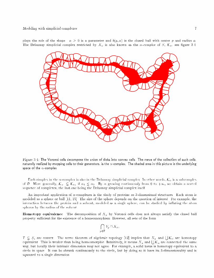
Modeling with simplicial complexes 7

plays the role of the shape. 0 is a parameter and b(p; ) is the closed ball with center p and radius .

The Delaunay simplicial complex restricted by X is also known as the -complex of S, K, see gure 3.4.

Figure 3.4: The Voronoi cells decompose the union of disks into convex cells. The nerve of the collection of such cells,naturally realized by mapping cells to their generators, is the -complex. The shaded area in this picture is the underlyingspace of the -complex.

Each simplex in the -complex is also in the Delaunay simplicial complex. In other words, K is a subcomplex

of D. More generally, K1 K2 if 1 2. By growing continuously from 0 to +1, we obtain a nested

sequence of complexes, the last one being the Delaunay simplicial complex itself.

An important application of -complexes is the study of proteins as 3-dimensional structures. Each atom is

modeled as a sphere or ball [11, 15]. The size of the sphere depends on the question of interest. For example, the

interaction between the protein and a solvent, modeled as a single sphere, can be studied by in ating the atom

spheres by the radius of the solvent.

Homotopy equivalence. The decomposition of X by Voronoi cells does not always satisfy the closed ball

property sucient for the existence of a homeomorphism. However, all sets of the form

\

p2T

Vp \X;

T S, are convex. The nerve theorem of algebraic topology [12] implies that X andSK are homotopy

equivalent. This is weaker than being homeomorphic. Intuitively, it means X andSK are connected the same

way, but locally their intrinsic dimension may not agree. For example, a solid torus is homotopy equivalent to a

circle in space. It can be shrunk continuously to the circle, but by doing so it loses its 3-dimensionality and is

squeezed to a single dimension.

Modeling with simplicial complexes 8

4 Conclusions

The purpose of this paper is to argue and partially demonstrate that simplicial complexes can serve as a general

geometric representation for a broad spectrum of modeling problems. This approach has tradition in combinatorial

topology, computational geometry, and grid generation. Indeed, the terms `triangulation' and `unstructured grid'

are often used as synonyms to `simplicial complex'. The study of simplicial complexes for modeling problems

is relatively recent, which is one of the reasons why this paper concentrates on the geometric and topological

fundamentals.

References

[1] D. K. Arrowsmith and C. M. Smith. Dynamical Systems. Dierential Equations, Maps, and Chaotic Behaviour.

Chapman and Hall, London, 1992.

[2] J. E. Castillo (ed.) Mathematical Aspects of Numerical Grid Generation. Society for Industrial and Applied Math-

ematics, Philadelphia, 1991.

[3] B. Delaunay. Sur la sphere vide. Izv. Akad. Nauk SSSR, Otdelenie Matematicheskii i Estestvennyka Nauk 7 (1934),793800.

[4] H. Edelsbrunner. The union of balls and its dual shape. In \Proc. 9th Ann. Sympos. Comput. Geom., 1993", 218231.

[5] H. Edelsbrunner and P. Fu. Measuring space lling diagrams and voids. Rept. UIUC-BI-MB-94-01, Beckman

Institute, Univ. Illinois, Urbana, 1994.

[6] H. Edelsbrunner and E. P. Mucke. Simulation of Simplicity: a technique to cope with degenerate cases in geometric

algorithms. ACM Trans. Comput. Graphics 9 (1990), 66104.

[7] H. Edelsbrunner and N. R. Shah. Triangulating topological spaces. In \Proc. 10th Ann. Sympos. Comput. Geom.1994", 285292.

[8] H. Fuchs, S. M. Kedem and S. P. Uselton. Optimal surface reconstruction from planar contours. Comm. ACM 20

(1977), 693702.

[9] W. Gellert, S. Gottwald, M. Hellwich, H. Kastner and H. Kustner. The VNR Concise Encyclopedia of

Mathematics. Second edition, van Nostrand Reinhold, New York, 1989.

[10] P. J. Giblin. Graphs, Surfaces, and Homology. 2nd edition, Chapman and Hall, London, 1981.

[11] B. Lee and F. M. Richards. The interpretation of protein structure: estimation of static accessibility. J. Mol. Biol.

55 (1971), 379400.

[12] J. Leray. Sur la forme des espaces topologiques et sur les points xes des representations. J. Math. Pure Appl. 24

(1945), 95167.

[13] J. R. Munkres. Elements of Algebraic Topology. Addison-Wesley, Redwood City, California, 1984.

[14] A. Paoluzzi, B. Bernardini, C. Cattani and V. Ferrucci. Dimension-independent modeling with simplicialcomplexes. ACM Trans. Graphics 12 (1993), 56102.

[15] F. M. Richards. Areas, volumes, packing, and protein structures. Ann. Rev. Biophys. Bioeng. 6 (1977), 151176.

[16] W. J. Schroeder and M. S. Shephard. A combined octree/Delaunay method for fully automatic 3-d mesh generation.

Internat. J. Numer. Meth. Engin. 29 (1990), 3755.

[17] G. F. Voronoi. Nouvelles applications des parametres continus a la theorie des formes quadratiques. J. Reine Angew.

Math. 133 (1907), 97178.

[18] C. K. Yap. Symbolic treatment of geometric degeneracies. J. Symbolic Comput. 10 (1990), 349370.

Polynomial Surface Patch Representations

Chandrajit L. Bajaj

Department of Computer Science,

Purdue University,

West Lafayette, Indiana 47907

Email: bajaj@cs.purdue.edu

http://www.cs.purdue.edu/people/bajaj

1 INTRODUCTION

Our approach to the design and analysis of geometric algorithms for operations on polynomial (algebraic) curves

and surfaces is to take the view of abstract data types, that is, a data representation coupled together with

the operations on them [7, 8]. In this framework, the choice of which representation of the polynomial curve or

surface patch to use is determined by the desired optimality of the geometric algorithms for the operations.

Polynomial curves and surfaces can be represented in an implicit form, and sometimes also in a parametric

form. The implicit form of a real polynomial surface in IR3 is

f(x; y; z) = 0 (1)

where f is a polynomial with coecients in IR. The parametric form, when it exists, for a real polynomial surface

in IR3 is

x =f1(s; t)

f4(s; t)

y =f2(s; t)

f4(s; t)

z =f3(s; t)

f4(s; t)(2)

where the fi are again polynomials with coecients in IR. The above implicit form describes a two dimensional

real algebraic variety (a surface) with a single polynomial equation in IR3. The parametric form also describes a

real two dimensional algebraic variety (a surface), however with a set of three independent polynomial equations

in IR5, with coordinate variables x; y; z; s; t. Alternatively, the parametric form of a real surface may also

be interpreted as a rational mapping from IR2 to IR3. We can thus compare the implicit and parametric

representations of polynomial surfaces by considering the the parametric form either as amapping or alternatively,an algebraic variety.

In these notes, we consider specic geometric operations of display/nite element mesh generation and data

tting, and compare the implicit and parametric polynomial forms for their superiority (or lack thereof) in

optimizing algorithms for operations in these categories.

Supported in part by NSF grant CCR 92-22467, AFOSR grant F49620-94-1-0080 and ONR grant N00014-94-1-0370

Section 2 sets the terminology and introduces some well known facts about polynomial curves and surfaces

and their patch representations. Section 3 compares the implicit and parametric surface representations for

graphics display and triangular mesh generation operations. Here the rational mapping gives an advantage to

the parametric form, though the algorithms to solve this problem in this representation are still non-trivial.

Section 4 considers the tradeo between implicit and parametric surface splines for interactive design and data

tting operations.

2 PRELIMINARIES

2.1 Mathematical Terminology

In this section we review some basic terminology from algebraic geometry that we shall use in subsequent sections.

These and additional facts can be found for example in [64, 68].

The set of real and complex solutions (or zero set Z(C)) of a collection C of polynomial equations

f1(x1; :::; xd) = 0

...

fm(x1; :::; xd) = 0 (3)

with coecients over the reals IR or complexes IC, is referred to as an algebraic set. The algebraic set dened

by a single equation (m = 1) is also known as a hypersurface. A algebraic set that cannot be represented as the

union of two other distinct algebraic sets, neither containing the other, is said to be irreducible. An irreducible

algebraic set Z(C) is also known as an algebraic variety V .A hypersurface in IRd, some d dimensional space, is of dimension d1. The dimension of an algebraic variety

V is k if its points can be put in (1; 1) rational correspondence with the points of an irreducible hypersurface

in k + 1 dimensional space. In IRd, a variety V1 of dimension k intersects a a variety V2 of dimension h, with

h d k, in an algebraic set Z(S) of dimension at least h+ k d. The resulting intersection is termed properif all subvarieties of Z(S) are of the same minimum dimension h + k n. Otherwise the intersection is termed

excess or improper. Let the algebraic degree of an algebraic variety V be the maximum degree of any dening

polynomial. A degree 1 hypersurface is also called a hyperplane while a degree 1 algebraic variety of dimension

k is also called a k- at. The geometric degree of a variety V of dimension k in some IRd is the maximumnumber

of intersections between V and a (d k)- at, counting both real and complex intersections and intersections

at innity. Hence the geometric degree of an algebraic hypersurface is the maximum number of intersections

between the hypersurface and a line, counting both real and complex intersections and at innity.

The following theorem, perhaps the oldest in algebraic geometry, summarizes the resulting geometric degree

of intersections of varieties of dierent degrees.

[Bezout] A variety of geometric degree p which properly intersects a variety of geometric degree q does so in an

algebraic set of geometric degree either at most pq or innity. 3

The normal or gradient of a hypersurface H : f(x1; :::; xn) = 0 is the vector rf = (fx1 ; fx2 ; : : : ; fxn). A point

p = (a0; a1; : : :an) on a hypersurface is a regular point if the gradient at p is not null; otherwise the point is

singular. A singular point q is of multiplicity e for a hypersurface H of degree d if any line through q meets

H in at most d e additional points. Similarly a singular point q is of multiplicity e for a variety V in IRn of

dimension k and degree d if any sub-space IRnk through q meets V in at most d e additional points. It is

important to note that even if two varieties intersect in a propermanner, their intersection in general may consist

of sub-varieties of various multiplicites. The total degree of the intersection, however is bounded by Bezout's

theorem. Finally, one notes that a hypersurface f(x1; :::; xn) = 0 of degree d has K =n+dn

coecients, which

is one more than the number of independent coecients. Hypersurfaces f(x1; :::; xn) = 0 of degree d form K 1

dimensional vector spaces over the eld of coecients of the polynomials.

Finally, two hypersurfaces f(x1; : : : ; xn) = 0 and g(x1; : : : ; xn) = 0 meet with Ck-continuity along a common

subvariety V if and only if there exist functions (x1; : : : ; xn) and (x1; : : : ; xn) such that all derivatives upto

order k of f g equals zero at all points along V , see for e.g., [36].

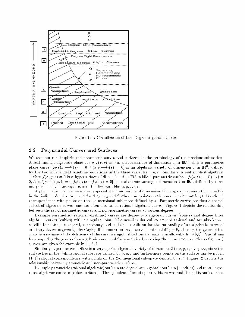
Implicit Quartics

Planar Implicit and Parametrics

Implicit Degree Eight

Implicit Degree Nine

Implicit Cubics

GEOMETRIC

DEGREE

1

2

3

4

8

9

Quadratic Implicit and Parametrics

Curves

Curves

Degree Nine Parametrics

Degree Eight Parametrics

Quartic Parametrics

CubicParametrics

SeparatingParametric andNon-parametricCurves

Figure 1: A Classication of Low Degree Algebraic Curves

2.2 Polynomial Curves and Surfaces

We cast our real implicit and parametric curves and surfaces, in the terminology of the previous subsection.

A real implicit algebraic plane curve f(x; y) = 0 is a hypersurface of dimension 1 in IR2, while a parametric

plane curve [f3(s)x f1(s) = 0; f3(s)y f2(s) = 0] is an algebraic variety of dimension 1 in IR3, dened

by the two independent algebraic equations in the three variables x; y; s. Similarly, a real implicit algebraic

surface f(x; y; z) = 0 is a hypersurface of dimension 2 in IR3, while a parametric surface [f4(s; t)x f1(s; t) =

0; f4(s; t)y f2(s; t) = 0; f4(s; t)z f3(s; t) = 0] is an algebraic variety of dimension 2 in IR5, dened by three

independent algebraic equations in the ve variables x; y; z; s; t.

A plane parametric curve is a very special algebraic variety of dimension 1 in x; y; s space, since the curve lies

in the 2-dimensional subspace dened by x; y and furthermore points on the curve can be put in (1; 1) rational

correspondence with points on the 1-dimensional sub-space dened by s. Parametric curves are thus a special

subset of algebraic curves, and are often also called rational algebraic curves. Figure 1 depicts the relationship

between the set of parametric curves and non-parametric curves at various degrees.

Example parametric (rational algebraic) curves are degree two algebraic curves (conics) and degree three

algebraic curves (cubics) with a singular point. The non-singular cubics are not rational and are also known

as elliptic cubics. In general, a necessary and sucient condition for the rationality of an algebraic curve of

arbitrary degree is given by the Cayley-Riemann criterion: a curve is rational i g = 0, where g, the genus of the

curve is a measure of the deciency of the curve's singularities from its maximumallowable limit [66]. Algorithms

for computing the genus of an algebraic curve and for symbolically deriving the parametric equations of genus 0

curves, are given for example in [1, 2, 3].

Similarly, a parametric surface is a very special algebraic variety of dimension 2 in x; y; z; s; t space, since the

surface lies in the 3-dimensional subspace dened by x; y; z and furthermore points on the surface can be put in

(1; 1) rational correspondence with points on the 2-dimensional sub-space dened by s; t. Figure 2 depicts the

relationship between parametric and non-parametric surfaces.

Example parametric (rational algebraic) surfaces are degree two algebraic surfaces (quadrics) and most degree

three algebraic surfaces (cubic surfaces). The cylinders of nonsingular cubic curves and the cubic surface cone

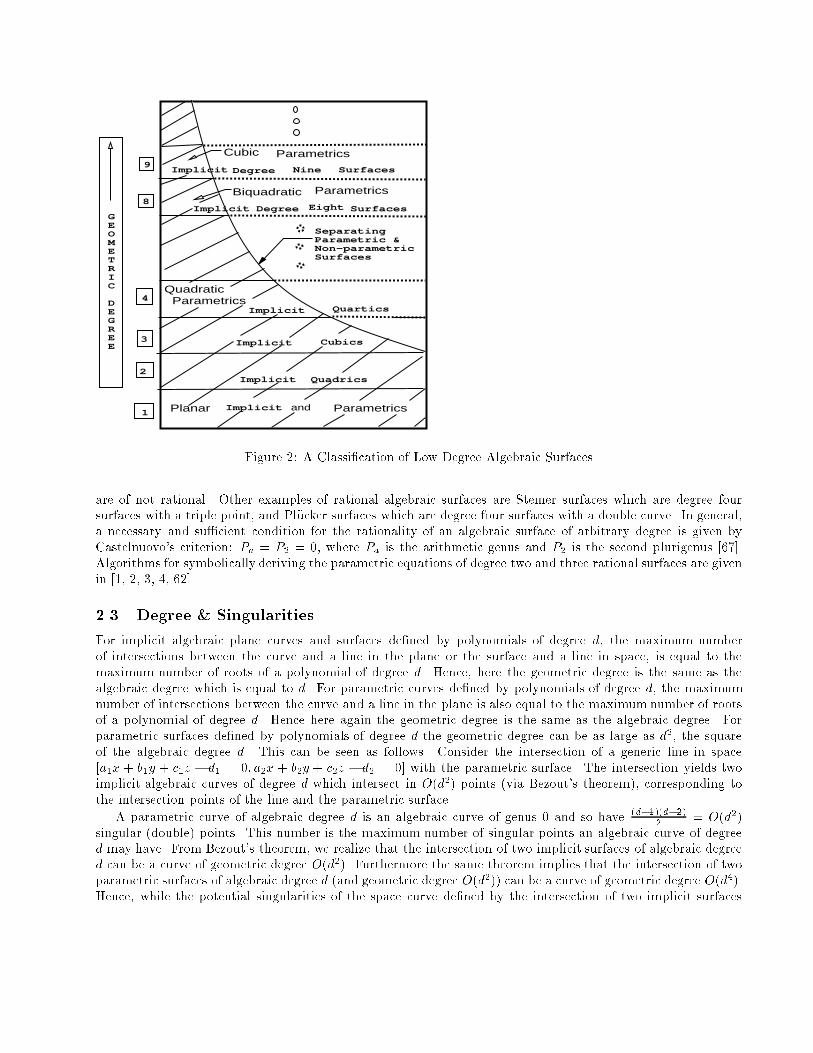
ParametricsQuadratic

Implicit Quartics

Planar Implicit and Parametrics

Cubic Parametrics

Biquadratic Parametrics

Implicit Degree Eight Surfaces

Implicit Degree Nine Surfaces

Implicit Cubics

Implicit Quadrics

GEOMETRIC

DEGREE

1

2

3

4

8

9

SeparatingParametric &Non-parametricSurfaces

Figure 2: A Classication of Low Degree Algebraic Surfaces

are of not rational. Other examples of rational algebraic surfaces are Steiner surfaces which are degree four

surfaces with a triple point, and Plucker surfaces which are degree four surfaces with a double curve. In general,

a necessary and sucient condition for the rationality of an algebraic surface of arbitrary degree is given by

Castelnuovo's criterion: Pa = P2 = 0, where Pa is the arithmetic genus and P2 is the second plurigenus [67].

Algorithms for symbolically deriving the parametric equations of degree two and three rational surfaces are given

in [1, 2, 3, 4, 62].

2.3 Degree & Singularities

For implicit algebraic plane curves and surfaces dened by polynomials of degree d, the maximum number

of intersections between the curve and a line in the plane or the surface and a line in space, is equal to the

maximum number of roots of a polynomial of degree d. Hence, here the geometric degree is the same as the

algebraic degree which is equal to d. For parametric curves dened by polynomials of degree d, the maximum

number of intersections between the curve and a line in the plane is also equal to the maximumnumber of roots

of a polynomial of degree d. Hence here again the geometric degree is the same as the algebraic degree. For

parametric surfaces dened by polynomials of degree d the geometric degree can be as large as d2, the square

of the algebraic degree d. This can be seen as follows. Consider the intersection of a generic line in space

[a1x + b1y + c1z d1 = 0; a2x + b2y + c2z d2 = 0] with the parametric surface. The intersection yields two

implicit algebraic curves of degree d which intersect in O(d2) points (via Bezout's theorem), corresponding to

the intersection points of the line and the parametric surface.

A parametric curve of algebraic degree d is an algebraic curve of genus 0 and so have(d1)(d2)

2= O(d2)

singular (double) points. This number is the maximum number of singular points an algebraic curve of degree

d may have. From Bezout's theorem, we realize that the intersection of two implicit surfaces of algebraic degree

d can be a curve of geometric degree O(d2). Furthermore the same theorem implies that the intersection of two

parametric surfaces of algebraic degree d (and geometric degree O(d2)) can be a curve of geometric degree O(d4).

Hence, while the potential singularities of the space curve dened by the intersection of two implicit surfaces

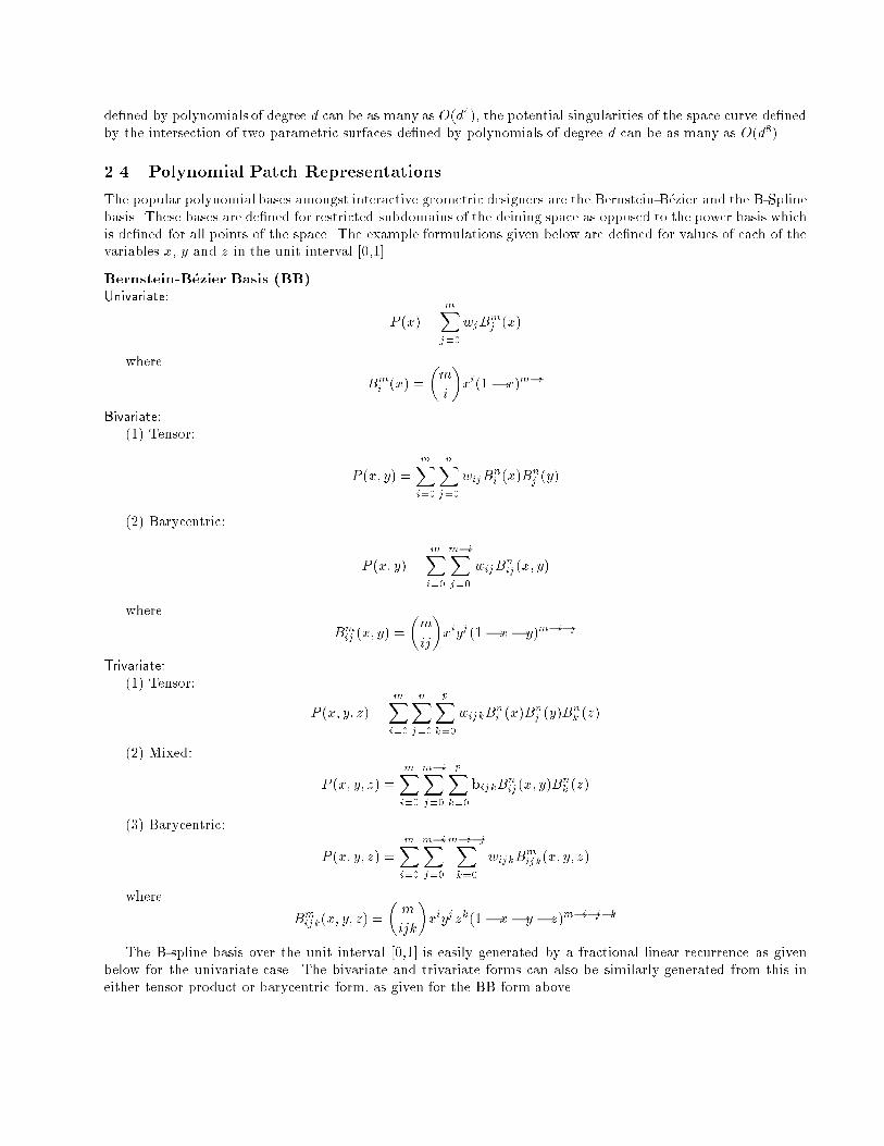
dened by polynomials of degree d can be as many as O(d4), the potential singularities of the space curve dened

by the intersection of two parametric surfaces dened by polynomials of degree d can be as many as O(d8).

2.4 Polynomial Patch Representations

The popular polynomial bases amongst interactive geometric designers are the Bernstein-Bezier and the B-Spline

basis. These bases are dened for restricted subdomains of the deining space as opposed to the power basis which

is dened for all points of the space. The example formulations given below are dened for values of each of the

variables x, y and z in the unit interval [0,1].

Bernstein-Bezier Basis (BB)

Univariate:

P (x) =

mXj=0

wjBmj (x)

where

Bmi (x) =

m

i

xi(1 x)mi

Bivariate:

(1) Tensor:

P (x; y) =

mXi=0

nXj=0

wijBni (x)B

nj (y)

(2) Barycentric:

P (x; y) =

mXi=0

miXj=0

wijBnij(x; y)

where

Bmij (x; y) =

m

ij

xiyj (1 x y)mij

Trivariate:

(1) Tensor:

P (x; y; z) =

mXi=0

nXj=0

pXk=0

wijkBni (x)B

nj (y)B

nk (z)

(2) Mixed:

P (x; y; z) =

mXi=0

miXj=0

pXk=0

bijkBnij(x; y)B

nk (z)

(3) Barycentric:

P (x; y; z) =

mXi=0

miXj=0

mijXk=0

wijkBmijk(x; y; z)

where

Bmijk(x; y; z) =

m

ijk

xiyjzk(1 x y z)mijk

The B-spline basis over the unit interval [0,1] is easily generated by a fractional linear recurrence as given

below for the univariate case. The bivariate and trivariate forms can also be similarly generated from this in

either tensor product or barycentric form, as given for the BB form above.

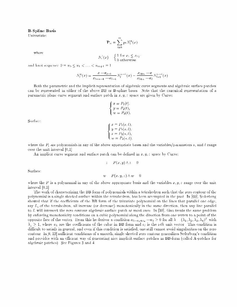
B-Spline Basis

Univariate:

Pn =

mXl=0

plNnl (x)

where

N1l (x) =

n1 for xl xl+10 otherwise.

and knot sequence 0 = u0 u1 < : : : < um+1 = 1

Nnl (x) =

x xl1

xl+n1 xl1Nn1l

(x) +xl+n x

xl+n xlNn1l+1 (x)

Both the parametric and the implicit representation of algebraic curve segments and algebraic surface patches

can be represented in either of the above BB or B-spline bases. Note that the canonical representation of a

parametric plane curve segment and surface patch in x; y; z space are given by Curve:8<:x = P1(t);

y = P2(t);

w = P3(t):

Surface: 8><>:x = P1(s; t);

y = P2(s; t);

z = P3(s; t);

w = P4(s; t):

where the Pi are polynomials in any of the above appropriate bases and the variables/parameters s, and t range

over the unit interval [0,1].

An implicit curve segment and surface patch can be dened in x; y; z space by Curve:

z = P (x; y) ^ z = 0

Surface:

w = P (x; y; z)^w = 0

where the P is a polynomial in any of the above appropriate basis and the variables x; y; z range over the unit

interval [0,1].

The work of characterizing the BB form of polynomials within a tetrahedron such that the zero contour of the

polynomial is a single sheeted surface within the tetrahedron, has been attempted in the past. In [60], Sederberg

showed that if the coecients of the BB form of the trivariate polynomial on the lines that parallel one edge,

say L, of the tetrahedron, all increase (or decrease) monotonically in the same direction, then any line parallel

to L will intersect the zero contour algebraic surface patch at most once. In [39], Guo treats the same problem

by enforcing monotonicity conditions on a cubic polynomial along the direction from one vertex to a point of the

opposite face of the vertex. From this he derives a condition ae1+e4 a 0 for all = (1; 2; 3; 4)T with

1 1, where a are the coecients of the cubic in BB form and ei is the i-th unit vector. This condition is

dicult to satisfy in general, and even if this condition is satised, one still cannot avoid singularities on the zero

contour. In[9, 12] sucient conditions of a smooth, single sheeted zero contour generalizes Sederberg's condition

and provides with an ecient way of generating nice implicit surface patches in BB-form (called A-patches for

algebraic patches). See Figures 3 and 4.

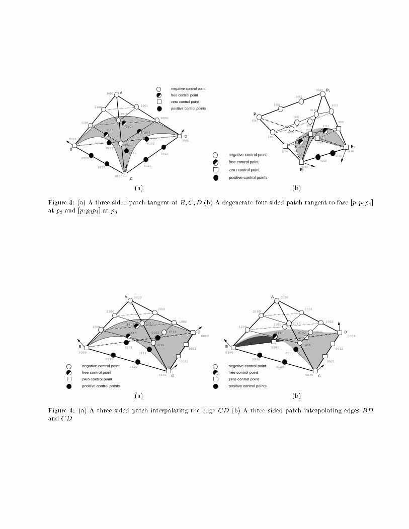
A

B

C

D

3000

2100

1200

0300

0210

0120

0030

0021

0012

0003

1002

2001

2010

1020 0102

0201

10111110

0111

1101

negative control point

free control point

positive control points

zero control point

negative control point

free control point

positive control points

zero control point

p

p

p

p

4

3

2

1

0300

0210

0120

0030

3000

2100

1200

2001

1002

0003

0012

0021

0102

02012010

1020

1101

1011 0111

1110

(a) (b)

Figure 3: (a) A three sided patch tangent at B;C;D (b) A degenerate four sided patch tangent to face [p1p2p4]

at p2 and [p1p3p4] at p3

A

B

C

D

3000

2100

1200

0300

0210

0120

0030

0021

0012

0003

10110102

0201

1110

0111

negative control point

free control point

positive control points

zero control point

2001

10022010

1020

1101

A

B

C

D

3000

2100

1200

0300

0210

0120

0030

0021

0012

0003

10110102

0201

1110

0111

negative control point

free control point

positive control points

zero control point

2001

10022010

1020

1101

(a) (b)

Figure 4: (a) A three sided patch interpolating the edge CD (b) A three sided patch interpolating edges BD

and CD

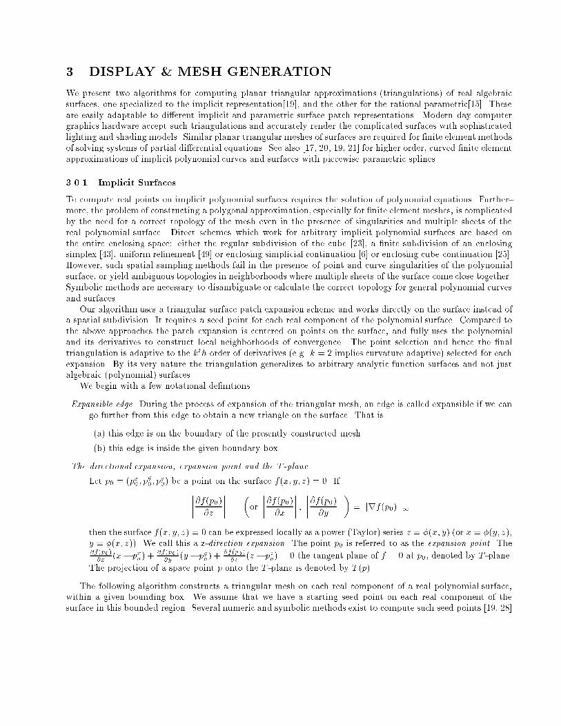
3 DISPLAY & MESH GENERATION

We present two algorithms for computing planar triangular approximations (triangulations) of real algebraic

surfaces, one specialized to the implicit representation[19], and the other for the rational parametric[15]. These

are easily adaptable to dierent implicit and parametric surface patch representations. Modern day computer

graphics hardware accept such triangulations and accurately render the complicated surfaces with sophisticated

lighting and shading models. Similar planar triangular meshes of surfaces are required for nite element methods

of solving systems of partial dierential equations. See also [17, 20, 19, 21] for higher order, curved nite element

approximations of implicit polynomial curves and surfaces with piecewise parametric splines.

3.0.1 Implicit Surfaces

To compute real points on implicit polynomial surfaces requires the solution of polynomial equations. Further-

more, the problem of constructing a polygonal approximation, especially for nite element meshes, is complicated

by the need for a correct topology of the mesh even in the presence of singularities and multiple sheets of the

real polynomial surface. Direct schemes which work for arbitrary implicit polynomial surfaces are based on

the entire enclosing space: either the regular subdivision of the cube [23], a nite subdivision of an enclosing

simplex [43], uniform renement [49] or enclosing simplicial continuation [6] or enclosing cube continuation [25].

However, such spatial sampling methods fail in the presence of point and curve singularities of the polynomial

surface, or yield ambiguous topologies in neighborhoods where multiple sheets of the surface come close together.

Symbolic methods are necessary to disambiguate or calculate the correct topology for general polynomial curves

and surfaces.

Our algorithm uses a triangular surface patch expansion scheme and works directly on the surface instead of

a spatial subdivision. It requires a seed point for each real component of the polynomial surface. Compared to

the above approaches the patch expansion is centered on points on the surface, and fully uses the polynomial

and its derivatives to construct local neighborhoods of convergence. The point selection and hence the nal

triangulation is adaptive to the kth order of derivatives (e.g. k = 2 implies curvature adaptive) selected for each

expansion. By its very nature the triangulation generalizes to arbitrary analytic function surfaces and not just

algebraic (polynomial) surfaces.

We begin with a few notational denitions

Expansible edge. During the process of expansion of the triangular mesh, an edge is called expansible if we can

go further from this edge to obtain a new triangle on the surface. That is

(a) this edge is on the boundary of the presently constructed mesh

(b) this edge is inside the given boundary box.

The directional expansion, expansion point and the T -plane.

Let p0 = (px0 ; py

0; pz0) be a point on the surface f(x; y; z) = 0. If@f(p0)@z

or

@f(p0)@x

;@f(p0)@y

= jjrf(p0)jj1

then the surface f(x; y; z) = 0 can be expressed locally as a power (Taylor) series z = (x; y) (or x = (y; z),

y = (x; z)). We call this a z-direction expansion. The point p0 is referred to as the expansion point. The@f(p0)

@x(x pxo ) +

@f(p0)

@y(y pyo) +

@f(p0)

@z(z pzo) = 0 the tangent plane of f = 0 at p0, denoted by T -plane.

The projection of a space point p onto the T -plane is denoted by T (p).

The following algorithm constructs a triangular mesh on each real component of a real polynomial surface,

within a given bounding box. We assume that we have a starting seed point on each real component of the

surface in this bounded region. Several numeric and symbolic methods exist to compute such seed points [19, 28]

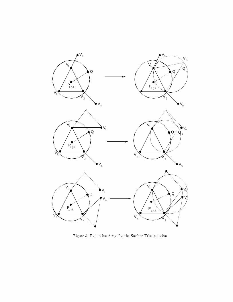
V

V

V

V

V

P

k

i

e

j

m

Q

ijk

V

V

V

V

i

e

j

m

Q

Pijk

Vn

Q1

V

V

V

V

P

k

i Ve

j

m

Q

ijk

V

V

V

i Ve

j

m

Q

Vk

Q1

V

V

V

P

k

i Ve

j

Vm

Q

ijk

V

V

i Ve

j

VmQ Q

Vk

Pijk

Figure 5: Expansion Steps for the Surface Triangulation

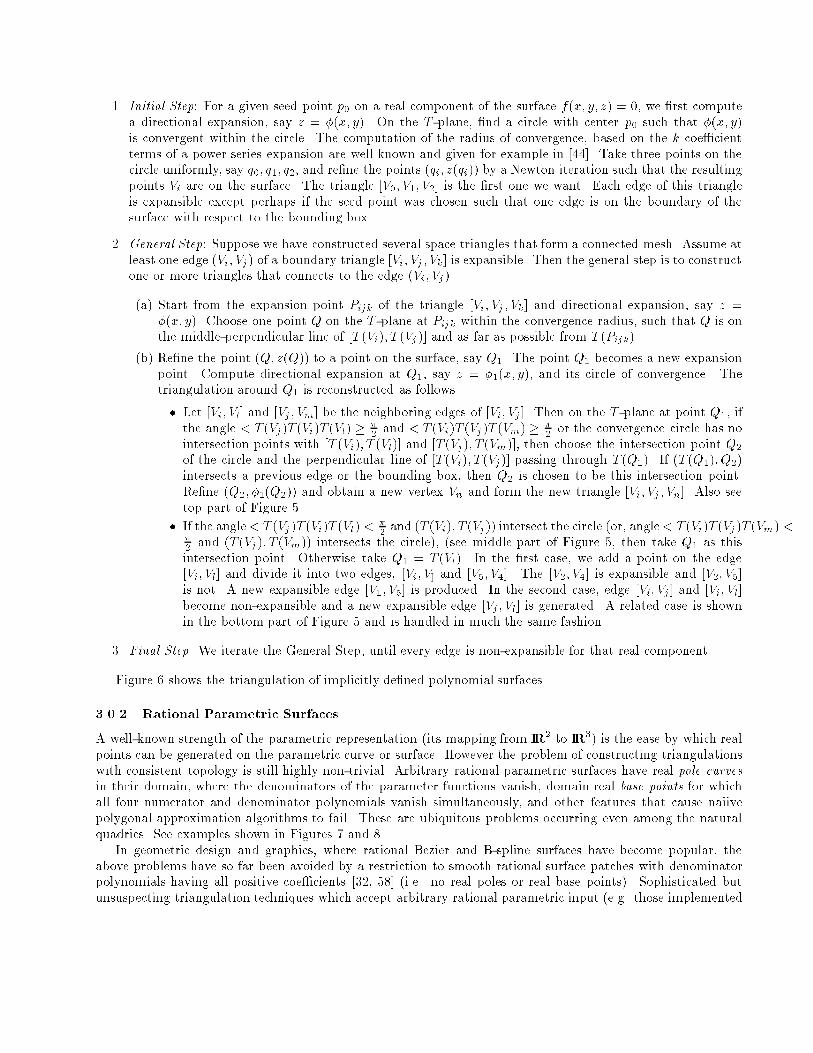
1. Initial Step: For a given seed point p0 on a real component of the surface f(x; y; z) = 0, we rst compute

a directional expansion, say z = (x; y). On the T -plane, nd a circle with center p0 such that (x; y)

is convergent within the circle. The computation of the radius of convergence, based on the k coecient

terms of a power series expansion are well known and given for example in [44]. Take three points on the

circle uniformly, say q0; q1; q2, and rene the points (qi; z(qi)) by a Newton iteration such that the resulting

points Vi are on the surface. The triangle [V0; V1; V2] is the rst one we want. Each edge of this triangle

is expansible except perhaps if the seed point was chosen such that one edge is on the boundary of the

surface with respect to the bounding box.

2. General Step: Suppose we have constructed several space triangles that form a connected mesh. Assume at

least one edge (Vi; Vj) of a boundary triangle [Vi; Vj; Vk] is expansible. Then the general step is to construct

one or more triangles that connects to the edge (Vi; Vj)

(a) Start from the expansion point Pijk of the triangle [Vi; Vj; Vk] and directional expansion, say z =

(x; y). Choose one point Q on the T -plane at Pijk within the convergence radius, such that Q is on

the middle-perpendicular line of [T (Vi); T (Vj)] and as far as possible from T (Pijk).

(b) Rene the point (Q; z(Q)) to a point on the surface, say Q1. The point Q1 becomes a new expansion

point. Compute directional expansion at Q1, say z = 1(x; y), and its circle of convergence. The

triangulation around Q1 is reconstructed as follows.

Let [Vi; Vl] and [Vj; Vm] be the neighboring edges of [Vi; Vj]. Then on the T -plane at point Q1, if

the angle < T (Vj)T (Vi)T (Vl)

2and < T (Vi)T (Vj)T (Vm)

2or the convergence circle has no

intersection points with [T (Vi); T (Vl)] and [T (Vj); T (Vm)], then choose the intersection point Q2

of the circle and the perpendicular line of [T (Vi); T (Vj)] passing through T (Q1). If (T (Q1); Q2)

intersects a previous edge or the bounding box, then Q2 is chosen to be this intersection point.

Rene (Q2; 1(Q2)) and obtain a new vertex Vn and form the new triangle [Vi; Vj; Vn]. Also see

top part of Figure 5.

If the angle< T (Vj)T (Vi)T (Vl) <

2and (T (Vi); T (Vj)) intersect the circle (or, angle< T (Vi)T (Vj)T (Vm) <

2and (T (Vj); T (Vm)) intersects the circle), (see middle part of Figure 5, then take Q1 as this

intersection point. Otherwise take Q1 = T (Vl). In the rst case, we add a point on the edge

[Vi; Vl] and divide it into two edges, [Vi; V] and [V5; V4]. The [V2; V4] is expansible and [V2; V5]

is not. A new expansible edge [V1; V5] is produced. In the second case, edge [Vi; Vj] and [Vi; Vl]

become non-expansible and a new expansible edge [Vj; Vl] is generated. A related case is shown

in the bottom part of Figure 5 and is handled in much the same fashion.

3. Final Step. We iterate the General Step, until every edge is non-expansible for that real component.

Figure 6 shows the triangulation of implicitly dened polynomial surfaces.

3.0.2 Rational Parametric Surfaces

A well-known strength of the parametric representation (its mapping from IR2 to IR3) is the ease by which real

points can be generated on the parametric curve or surface. However the problem of constructing triangulations

with consistent topology is still highly non-trivial. Arbitrary rational parametric surfaces have real pole curvesin their domain, where the denominators of the parameter functions vanish, domain real base points for whichall four numerator and denominator polynomials vanish simultaneously, and other features that cause naiive

polygonal approximation algorithms to fail. These are ubiquitous problems occurring even among the natural

quadrics. See examples shown in Figures 7 and 8.

In geometric design and graphics, where rational Bezier and B-spline surfaces have become popular, the

above problems have so far been avoided by a restriction to smooth rational surface patches with denominator

polynomials having all positive coecients [32, 58] (i.e. no real poles or real base points). Sophisticated but

unsuspecting triangulation techniques which accept arbitrary rational parametric input (e.g. those implemented

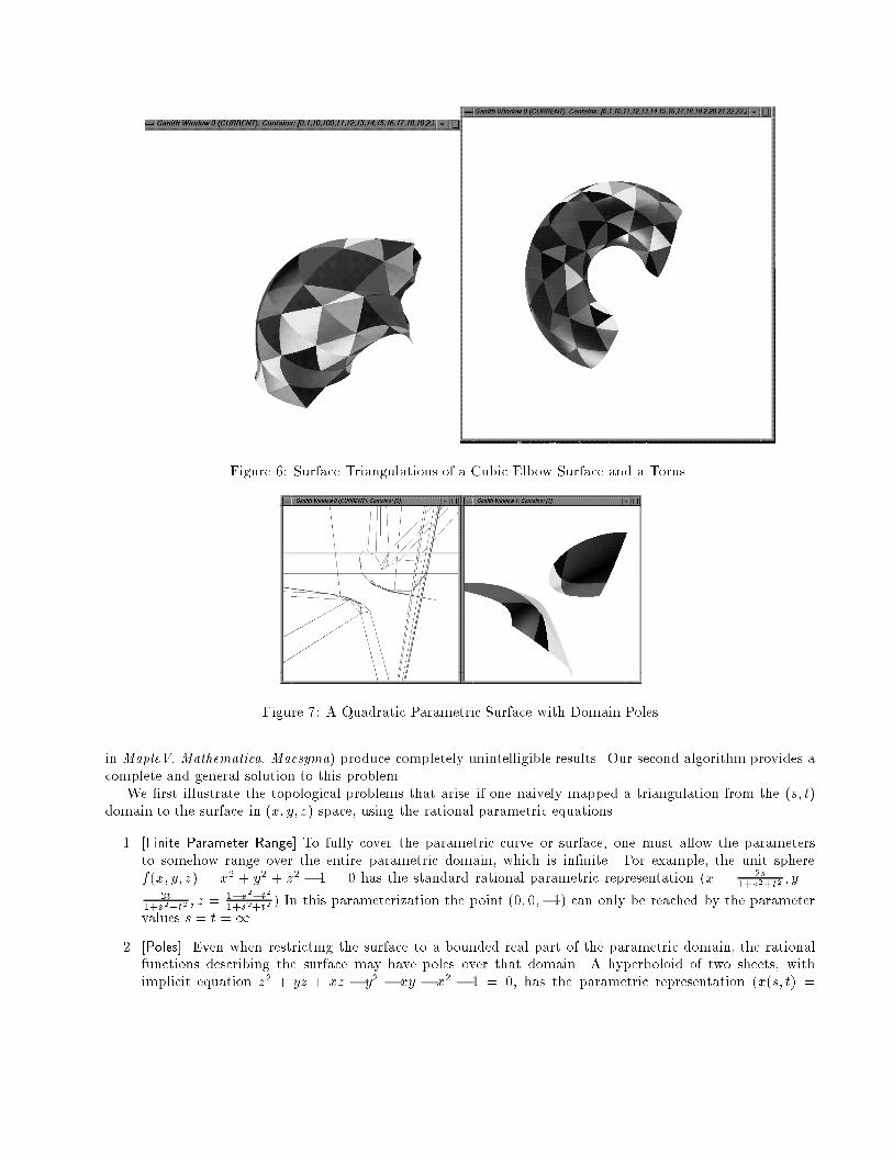
Figure 6: Surface Triangulations of a Cubic Elbow Surface and a Torus

Figure 7: A Quadratic Parametric Surface with Domain Poles

in MapleV, Mathematica, Macsyma) produce completely unintelligible results. Our second algorithm provides a

complete and general solution to this problem.

We rst illustrate the topological problems that arise if one naively mapped a triangulation from the (s; t)

domain to the surface in (x; y; z) space, using the rational parametric equations.

1. [Finite Parameter Range] To fully cover the parametric curve or surface, one must allow the parameters

to somehow range over the entire parametric domain, which is innite. For example, the unit sphere

f(x; y; z) = x2 + y2 + z2 1 = 0 has the standard rational parametric representation (x = 2s1+s2+t2

; y =2t

1+s2+t2; z = 1s2t2

1+s2+t2) In this parameterization the point (0; 0;1) can only be reached by the parameter

values s = t =1.

2. [Poles] Even when restricting the surface to a bounded real part of the parametric domain, the rational

functions describing the surface may have poles over that domain. A hyperboloid of two sheets, with

implicit equation z2 + yz + xz y2 xy x2 1 = 0, has the parametric representation (x(s; t) =

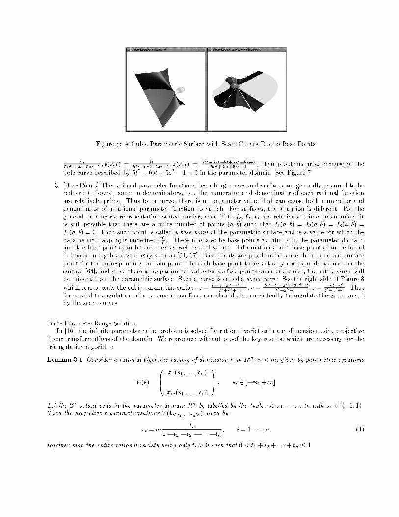
Figure 8: A Cubic Parametric Surface with Seam Curves Due to Base Points

4s5t2+6st+5s21

; y(s; t) = 4t5t2+6st+5s21

; z(s; t) = 5t2+6st2t+5s22s+15t2+6st+5s21

) then problems arise because of the

pole curve described by 5t2 + 6st+ 5s2 1 = 0 in the parameter domain. See Figure 7.

3. [Base Points] The rational parameter functions describing curves and surfaces are generally assumed to be

reduced to lowest common denominators, i.e., the numerator and denominator of each rational function

are relatively prime. Thus for a curve, there is no parameter value that can cause both numerator and

denominator of a rational parameter function to vanish. For surfaces, the situation is dierent. For the

general parametric representation stated earlier, even if f1; f2; f3; f4 are relatively prime polynomials, it

is still possible that there are a nite number of points (a; b) such that f1(a; b) = f2(a; b) = f3(a; b) =

f4(a; b) = 0. Each such point is called a base point of the parametric surface and is a value for which the

parametric mapping is undened (00). There may also be base points at innity in the parameter domain,

and the base points can be complex as well as real-valued. Information about base points can be found

in books on algebraic geometry such as [64, 67]. Base points are problematic since there is no one surface

point for the corresponding domain point. To each base point there actually corresponds a curve on the

surface [64], and since there is no parameter value for surface points on such a curve, the entire curve will

be missing from the parametric surface. Such a curve is called a seam curve. See the right side of Figure 8

which corresponds the cubic parametric surface x = t3t+s3s2+1t3+s3+1

; y = 2t3t2s2t+2s3+2t3+s3+1

; z = sts3

t3+s3+1. Thus

for a valid triangulation of a parametric surface, one should also consistently triangulate the gaps caused

by the seam curves.

Finite Parameter Range Solution

In [16], the innite parameter value problem is solved for rational varieties in any dimension using projective

linear transformations of the domain. We reproduce without proof the key results, which are necessary for the

triangulation algorithm.

Lemma 3.1 Consider a rational algebraic variety of dimension n in Rm, n < m, given by parametric equations

V (s) =

0B@

x1(s1; : : : ; sn)...

xm(s1; : : : ; sn)

1CA ; si 2 [1;+1]

Let the 2n octant cells in the parameter domain Rn be labelled by the tuples < 1; : : :n > with i 2 f1; 1g.Then the projective reparameterizations V (t<1;:::;n>) given by

si = iti

1 t1 t2 : : : tn; i = 1; : : : ; n (4)

together map the entire rational variety using only ti 0 such that 0 t1 + t2 + : : :+ tn 1.

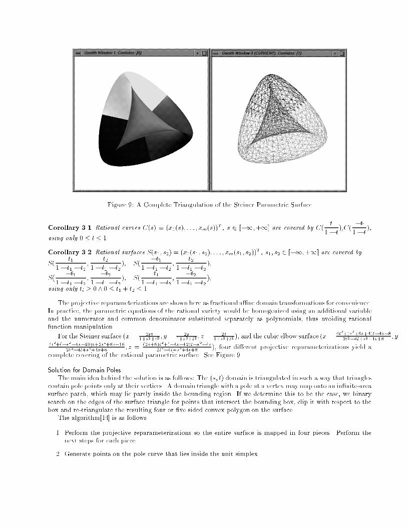
Figure 9: A Complete Triangulation of the Steiner Parametric Surface

Corollary 3.1 Rational curves C(s) = (x1(s); : : : ; xm(s))T , s 2 [1;+1] are covered by C(

t

1 t),C(

t

1 t),

using only 0 t 1.

Corollary 3.2 Rational surfaces S(s1; s2) = (x1(s1; s2); : : : ; xm(s1; s2))T , s1; s2 2 [1;+1] are covered by

S(t1

1 t1 t2;

t2

1 t1 t2), S(

t1

1 t1 t2;

t2

1 t1 t2),

S(t1

1 t1 t2;

t2

1 t1 t2), S(

t1

1 t1 t2;

t2

1 t1 t2),

using only ti 0 ^ 0 t1 + t2 1.

The projective reparameterizations are shown here as fractional ane domain transformations for convenience.

In practice, the parametric equations of the rational variety would be homogenized using an additional variable

and the numerator and common denominator substituted separately as polynomials, thus avoiding rational

function manipulation.

For the Steiner surface (x = 2st1+s2+t2

; y = 2s1+s2+t2

; z = 2t1+s2+t2

), and the cubic elbow surface (x =4t2+(s2+6s+4)t4s8

2t24t+s2+4s+8; y =

4t2+(s26s20)t+2s2+8s+16

2t24t+s2+4s+8; z =

(2s+6)t2+(4s12)ts24s

2t24t+s2+4s+8), four dierent projective reparameterizations yield a

complete covering of the rational parametric surface. See Figure 9.

Solution for Domain Poles

The main idea behind the solution is as follows: The (s; t) domain is triangulated in such a way that triangles

contain pole points only at their vertices. A domain triangle with a pole at a vertex maymap onto an innite-area

surface patch, which may lie partly inside the bounding region. If we determine this to be the case, we binary

search on the edges of the surface triangle for points that intersect the bounding box, clip it with respect to the

box and re-triangulate the resulting four or ve sided convex polygon on the surface.

The algorithm[14] is as follows.

1. Perform the projective reparameterizations so the entire surface is mapped in four pieces. Perform the

next steps for each piece.

2. Generate points on the pole curve that lies inside the unit simplex.

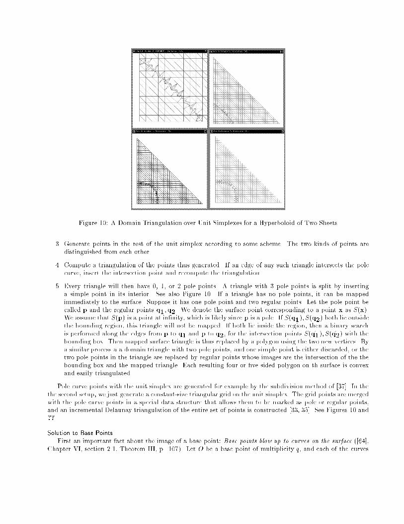
Figure 10: A Domain Triangulation over Unit Simplexes for a Hyperboloid of Two Sheets

3. Generate points in the rest of the unit simplex according to some scheme. The two kinds of points are

distinguished from each other.

4. Compute a triangulation of the points thus generated. If an edge of any such triangle intersects the pole

curve, insert the intersection point and recompute the triangulation.

5. Every triangle will then have 0, 1, or 2 pole points. A triangle with 3 pole points is split by inserting

a simple point in its interior. See also Figure 10. If a triangle has no pole points, it can be mapped

immediately to the surface. Suppose it has one pole point and two regular points. Let the pole point be

called p and the regular points q1;q2. We denote the surface point corresponding to a point x as S(x).

We assume that S(p) is a point at innity, which is likely since p is a pole. If S(q1); S(q2) both lie outside

the bounding region, this triangle will not be mapped. If both lie inside the region, then a binary search

is performed along the edges from p to q1 and p to q2, for the intersection points S(q1); S(q2) with the

bounding box. Then mapped surface triangle is thus replaced by a polygon using the two new vertices. By

a similar process a a domain triangle with two pole points, and one simple point is either discarded, or the

two pole points in the triangle are replaced by regular points whose images are the intersection of the the

bounding box and the mapped triangle. Each resulting four or ve sided polygon on th surface is convex

and easily triangulated.

Pole curve points with the unit simplex are generated for example by the subdivision method of [37]. In the

the second setup, we just generate a constant-size triangular grid on the unit simplex. The grid points are merged

with the pole curve points in a special data structure that allows them to be marked as pole or regular points,

and an incremental Delaunay triangulation of the entire set of points is constructed [33, 35]. See Figures 10 and

??.

Solution to Base Points

First an important fact about the image of a base point: Base points blow up to curves on the surface ([64],Chapter VI, section 2.1, Theorem III, p. 107). Let O be a base point of multiplicity q, and each of the curves

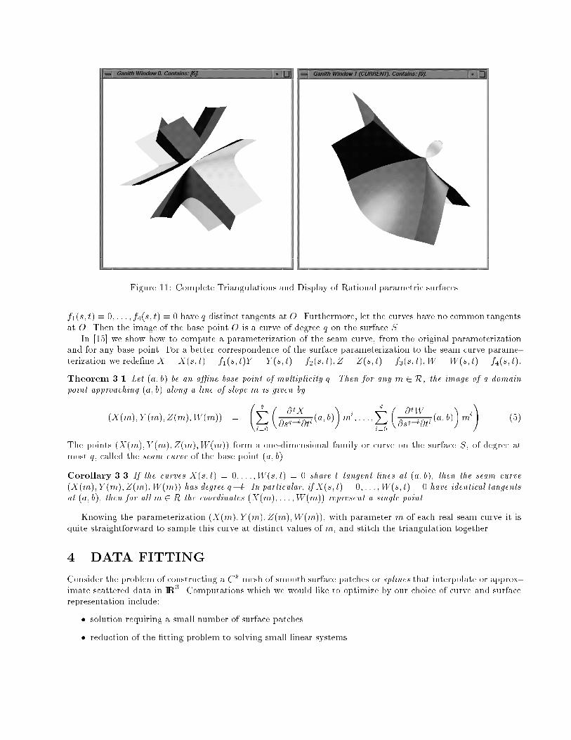
Figure 11: Complete Triangulations and Display of Rational parametric surfaces

f1(s; t) = 0; : : : ; f4(s; t) = 0 have q distinct tangents at O. Furthermore, let the curves have no common tangents

at O. Then the image of the base point O is a curve of degree q on the surface S.

In [15] we show how to compute a parameterization of the seam curve, from the original parameterization

and for any base point. For a better correspondence of the surface parameterization to the seam curve parame-

terization we redene X = X(s; t) = f1(s; t)Y = Y (s; t) = f2(s; t); Z = Z(s; t) = f3(s; t);W = W (s; t) = f4(s; t):

Theorem 3.1 Let (a; b) be an ane base point of multiplicity q. Then for any m 2 R, the image of a domainpoint approaching (a; b) along a line of slope m is given by

(X(m); Y (m); Z(m);W (m)) =

qX

i=0

@qX

@sqi@ti(a; b)

mi; : : : ;

qXi=0

@qW

@sqi@ti(a; b)

mi

!(5)

The points (X(m); Y (m); Z(m);W (m)) form a one-dimensional family or curve on the surface S, of degree at

most q, called the seam curve of the base point (a; b).

Corollary 3.3 If the curves X(s; t) = 0; : : : ;W (s; t) = 0 share t tangent lines at (a; b), then the seam curve(X(m); Y (m); Z(m);W (m)) has degree qt. In particular, if X(s; t) = 0; : : : ;W (s; t) = 0 have identical tangentsat (a; b), then for all m 2 R the coordinates (X(m); : : : ;W (m)) represent a single point.

Knowing the parameterization (X(m); Y (m); Z(m);W (m)), with parameter m of each real seam curve it is

quite straightforward to sample this curve at distinct values of m, and stitch the triangulation together.

4 DATA FITTING

Consider the problem of constructing a Ck mesh of smooth surface patches or splines that interpolate or approx-imate scattered data in IR3. Computations which we would like to optimize by our choice of curve and surface

representation include:

solution requiring a small number of surface patches

reduction of the tting problem to solving small linear systems

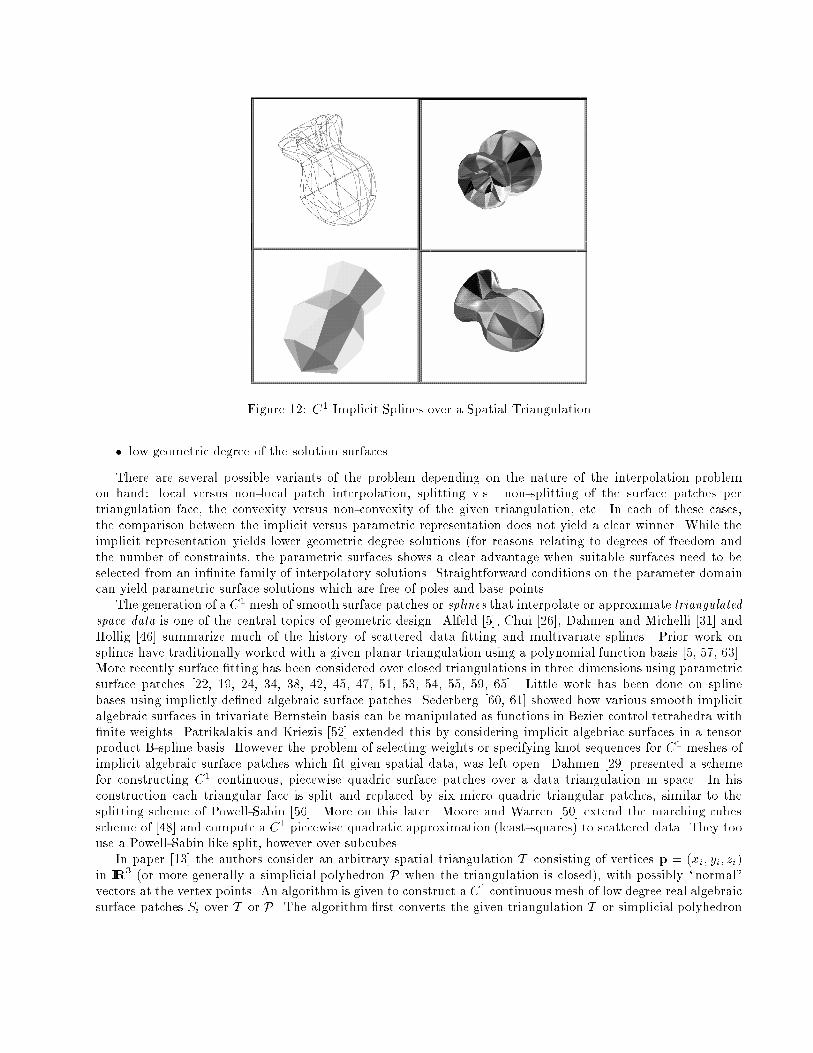
Figure 12: C1 Implicit Splines over a Spatial Triangulation

low geometric degree of the solution surfaces

There are several possible variants of the problem depending on the nature of the interpolation problem

on hand: local versus non-local patch interpolation, splitting v.s. non-splitting of the surface patches per

triangulation face, the convexity versus non-convexity of the given triangulation, etc. In each of these cases,

the comparison between the implicit versus parametric representation does not yield a clear winner. While the

implicit representation yields lower geometric degree solutions (for reasons relating to degrees of freedom and

the number of constraints, the parametric surfaces shows a clear advantage when suitable surfaces need to be

selected from an innite family of interpolatory solutions. Straightforward conditions on the parameter domain

can yield parametric surface solutions which are free of poles and base points.

The generation of a C1 mesh of smooth surface patches or splines that interpolate or approximate triangulatedspace data is one of the central topics of geometric design. Alfeld [5], Chui [26], Dahmen and Michelli [31] and

Hollig [46] summarize much of the history of scattered data tting and multivariate splines. Prior work on

splines have traditionally worked with a given planar triangulation using a polynomial function basis [5, 57, 63].

More recently surface tting has been considered over closed triangulations in three dimensions using parametric

surface patches [22, 19, 24, 34, 38, 42, 45, 47, 51, 53, 54, 55, 59, 65]. Little work has been done on spline

bases using implictly dened algebraic surface patches. Sederberg [60, 61] showed how various smooth implicit

algebraic surfaces in trivariate Bernstein basis can be manipulated as functions in Bezier control tetrahedra with

nite weights. Patrikalakis and Kriezis [52] extended this by considering implicit algebriac surfaces in a tensor

product B-spline basis. However the problem of selecting weights or specifying knot sequences for C1 meshes of

implicit algebraic surface patches which t given spatial data, was left open. Dahmen [29] presented a scheme

for constructing C1 continuous, piecewise quadric surface patches over a data triangulation in space. In his

construction each triangular face is split and replaced by six micro quadric triangular patches, similar to the

splitting scheme of Powell-Sabin [56]. More on this later. Moore and Warren [50] extend the marching cubes

scheme of [48] and compute a C1 piecewise quadratic approximation (least-squares) to scattered data. They too

use a Powell-Sabin like split, however over subcubes.

In paper [13] the authors consider an arbitrary spatial triangulation T consisting of vertices p = (xi; yi; zi)

in IR3 (or more generally a simplicial polyhedron P when the triangulation is closed), with possibly \normal"

vectors at the vertex points. An algorithm is given to construct a C1 continuous mesh of low degree real algebraic

surface patches Si over T or P. The algorithm rst converts the given triangulation T or simplicial polyhedron

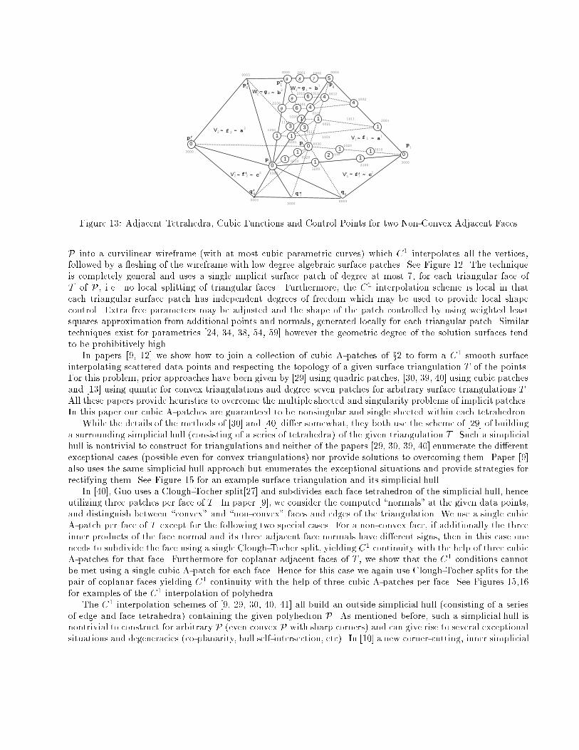
1

p

p

p"p’

qq’

2

3

4

4 4

p4

0003 0003

3000

3000

03001200

21000210

0120

0030 10202010

1110

0201

1101

20011011

0021

0102

1002

0012

00030003

3000

2010 1011

11012100

1020

1110

1200

10022001

0111

1

V

WW

V

V V’’

21

1

12

2 ~

~ ~

~

~~

f

f’ f’

f

gg

2

2

1

12

~ a

~ c ~ c

~ a

~ b~ b

2

21

1

121

p’

p1

10 0

0

01

1

11

11

1 1

12

3 3

44

4

6

5

3000

q "1

1

6

89

9

9

7

Figure 13: Adjacent Tetrahedra, Cubic Functions and Control Points for two Non-Convex Adjacent Faces

P into a curvilinear wireframe (with at most cubic parametric curves) which C1 interpolates all the vertices,

followed by a eshing of the wireframe with low degree algebraic surface patches. See Figure 12. The technique

is completely general and uses a single implicit surface patch of degree at most 7, for each triangular face of

T of P, i.e. no local splitting of triangular faces. Furthermore, the C1 interpolation scheme is local in that

each triangular surface patch has independent degrees of freedom which may be used to provide local shape

control. Extra free parameters may be adjusted and the shape of the patch controlled by using weighted least

squares approximation from additional points and normals, generated locally for each triangular patch. Similar

techniques exist for parametrics [24, 34, 38, 54, 59] however the geometric degree of the solution surfaces tend

to be prohibitively high.

In papers [9, 12] we show how to join a collection of cubic A-patches of x2 to form a C1 smooth surface

interpolating scattered data points and respecting the topology of a given surface triangulation T of the points.

For this problem, prior approaches have been given by [29] using quadric patches, [30, 39, 40] using cubic patches

and [13] using quintic for convex triangulations and degree seven patches for arbitrary surface triangulations T .

All these papers provide heuristics to overcome the multiple sheeted and singularity problems of implicit patches.

In this paper our cubic A-patches are guaranteed to be nonsingular and single sheeted within each tetrahedron.

While the details of the methods of [30] and [40] dier somewhat, they both use the scheme of [29] of building

a surrounding simplicial hull (consisting of a series of tetrahedra) of the given triangulation T . Such a simplicial

hull is nontrivial to construct for triangulations and neither of the papers [29, 30, 39, 40] enumerate the dierent

exceptional cases (possible even for convex triangulations) nor provide solutions to overcoming them. Paper [9]

also uses the same simplicial hull approach but enumerates the exceptional situations and provide strategies for

rectifying them. See Figure 15 for an example surface triangulation and its simplicial hull.

In [40], Guo uses a Clough-Tocher split[27] and subdivides each face tetrahedron of the simplicial hull, hence

utilizing three patches per face of T . In paper [9], we consider the computed \normals" at the given data points,

and distinguish between \convex" and \non-convex" faces and edges of the triangulation. We use a single cubic

A-patch per face of T except for the following two special cases. For a non-convex face, if additionally the three

inner products of the face normal and its three adjacent face normals have dierent signs, then in this case one

needs to subdivide the face using a single Clough-Tocher split, yielding C1 continuity with the help of three cubic

A-patches for that face. Furthermore for coplanar adjacent faces of T , we show that the C1 conditions cannot

be met using a single cubic A-patch for each face. Hence for this case we again use Clough-Tocher splits for the

pair of coplanar faces yielding C1 continuity with the help of three cubic A-patches per face. See Figures 15,16

for examples of the C1 interpolation of polyhedra.

The C1 interpolation schemes of [9, 29, 30, 40, 41] all build an outside simplicial hull (consisting of a series

of edge and face tetrahedra) containing the given polyhedron P. As mentioned before, such a simplicial hull is

nontrivial to construct for arbitrary P (even convex P with sharp corners) and can give rise to several exceptional

situations and degeneracies (co-planarity, hull self-intersection, etc). In [10] a new corner-cutting, inner simplicial

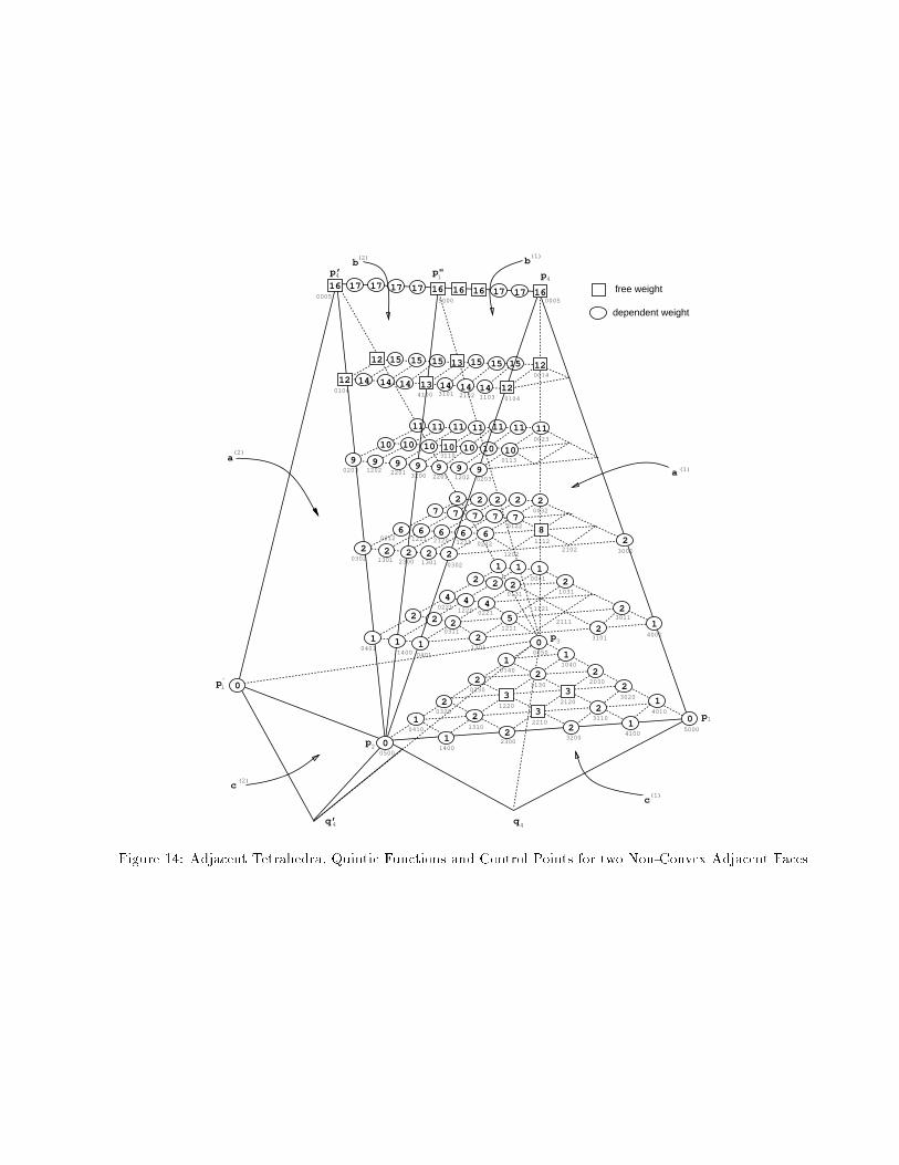
0

1

11

1

1

1 1

2 2

2

2

2

2

2

2 2

2

2

2

22

2

22

2 2 2

22

22

3

3

3

444

5

66 666

7 77 77

8

9999

1010101010

10

11 111111 11 1111

121213

10

141414141414

1515 1515 1515

161617 1717 17 1717

p

p

p

p

p

1’

2

1

4p’4 1

3

free weight

dependent weight

05001400

23003200

50000410 13102210

31104010

3020

2030

1040

0050

4100

03201220

2120

02301130

0140

040114000401

40013101

1301

0041

0005

3002

1112

0032

0023

0014

0104

0203

0302

0212

0122

0311

0221

0131

1211

1121

21113011

1031

0113

0302 2300 13011301

0203 1202 2201 3200 2201 1202

01044100 3101 2102 1103

0212 1211 2120 1211

00055000

3110

q’ q4 4

12022102

1

2

9

12

16

1

2

9

12

16

2

1

0

16

13

9

2

1

0

0

12 2 1

p"

12200221

a (1)

(2)a

bb

c

c

(2) (1)

(1)

(2)

Figure 14: Adjacent Tetrahedra, Quintic Functions and Control Points for two Non-Convex Adjacent Faces

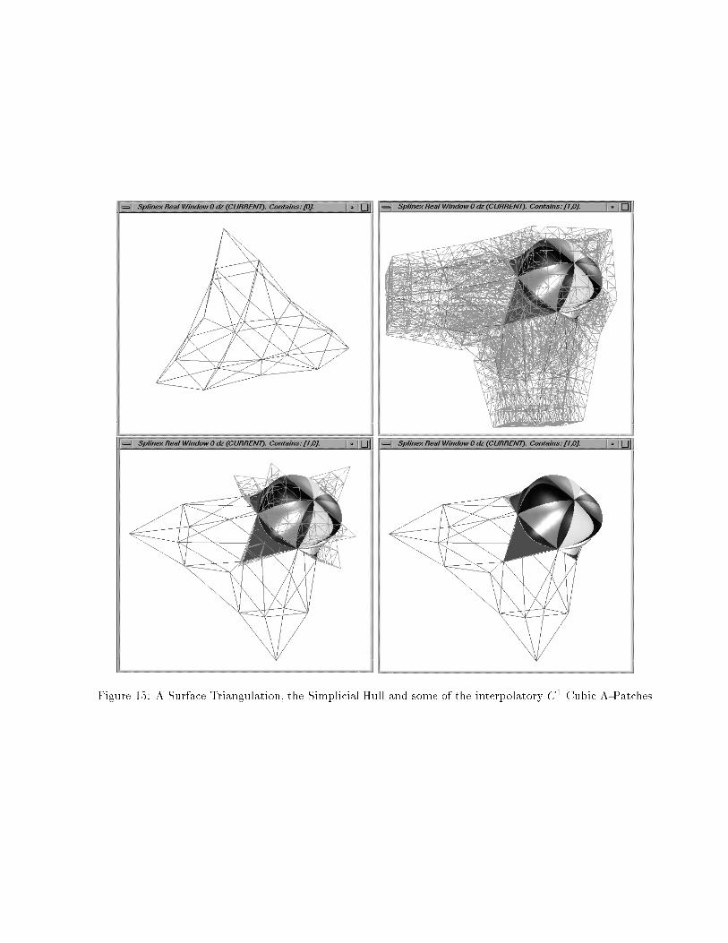
Figure 15: A Surface Triangulation, the Simplicial Hull and some of the interpolatory C1 Cubic A-Patches

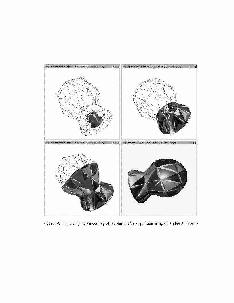
Figure 16: The Complete Smoothing of the Surface Triangulation using C1 Cubic A-Patches

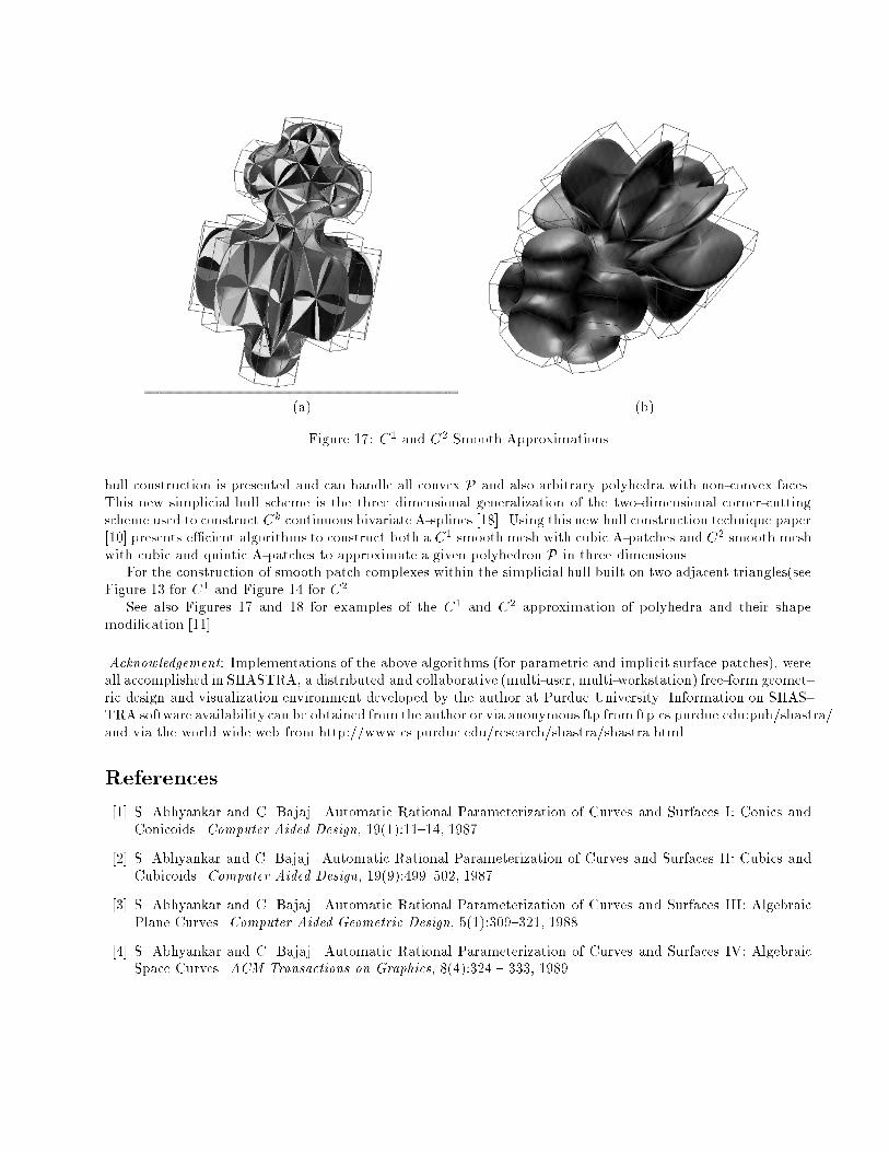
(a) (b)

Figure 17: C1 and C2 Smooth Approximations

hull construction is presented and can handle all convex P and also arbitrary polyhedra with non-convex faces.

This new simplicial hull scheme is the three dimensional generalization of the two-dimensional corner-cutting

scheme used to construct Ck continuous bivariate A-splines [18]. Using this new hull construction technique paper

[10] presents ecient algorithms to construct both a C1 smooth mesh with cubic A-patches and C2 smooth mesh

with cubic and quintic A-patches to approximate a given polyhedron P in three dimensions.

For the construction of smooth patch complexes within the simplicial hull built on two adjacent triangles(see

Figure 13 for C1 and Figure 14 for C2.

See also Figures 17 and 18 for examples of the C1 and C2 approximation of polyhedra and their shape

modication [11].

Acknowledgement: Implementations of the above algorithms (for parametric and implicit surface patches), were

all accomplished in SHASTRA, a distributed and collaborative (multi-user, multi-workstation) free-form geomet-

ric design and visualization environment developed by the author at Purdue University. Information on SHAS-

TRA software availability can be obtained from the author or via anonymous ftp from ftp.cs.purdue.edu:pub/shastra/

and via the world wide web from http://www.cs.purdue.edu/research/shastra/shastra.html.

References

[1] S. Abhyankar and C. Bajaj. Automatic Rational Parameterization of Curves and Surfaces I: Conics and

Conicoids. Computer Aided Design, 19(1):1114, 1987.

[2] S. Abhyankar and C. Bajaj. Automatic Rational Parameterization of Curves and Surfaces II: Cubics and

Cubicoids. Computer Aided Design, 19(9):499502, 1987.

[3] S. Abhyankar and C. Bajaj. Automatic Rational Parameterization of Curves and Surfaces III: Algebraic

Plane Curves. Computer Aided Geometric Design, 5(1):309321, 1988.

[4] S. Abhyankar and C. Bajaj. Automatic Rational Parameterization of Curves and Surfaces IV: Algebraic

Space Curves. ACM Transactions on Graphics, 8(4):324 333, 1989.

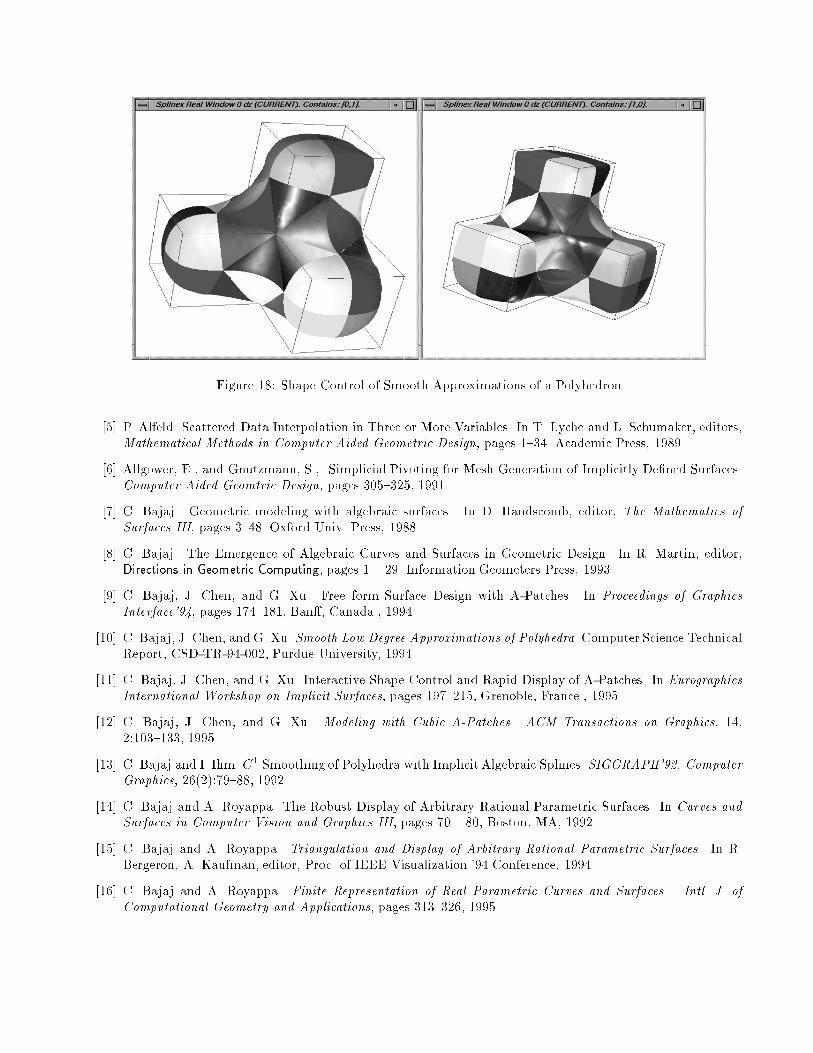
Figure 18: Shape Control of Smooth Approximations of a Polyhedron

[5] P. Alfeld. Scattered Data Interpolation in Three or More Variables. In T. Lyche and L. Schumaker, editors,

Mathematical Methods in Computer Aided Geometric Design, pages 134. Academic Press, 1989.

[6] Allgower, E., and Gnutzmann, S.,. Simplicial Pivoting for Mesh Generation of Implicitly Dened Surfaces.

Computer Aided Geomtric Design, pages 305325, 1991.

[7] C. Bajaj. Geometric modeling with algebraic surfaces. In D. Handscomb, editor, The Mathematics ofSurfaces III, pages 348. Oxford Univ. Press, 1988.

[8] C. Bajaj. The Emergence of Algebraic Curves and Surfaces in Geometric Design. In R. Martin, editor,

Directions in Geometric Computing, pages 1 29. Information Geometers Press, 1993.

[9] C. Bajaj, J. Chen, and G. Xu. Free form Surface Design with A-Patches. In Proceedings of GraphicsInterface'94, pages 174181, Ban, Canada., 1994.

[10] C. Bajaj, J. Chen, and G. Xu. Smooth Low Degree Approximations of Polyhedra. Computer Science Technical

Report, CSD-TR-94-002, Purdue University, 1994.

[11] C. Bajaj, J. Chen, and G. Xu. Interactive Shape Control and Rapid Display of A-Patches. In EurographicsInternational Workshop on Implicit Surfaces, pages 197215, Grenoble, France., 1995.

[12] C. Bajaj, J. Chen, and G. Xu. Modeling with Cubic A-Patches. ACM Transactions on Graphics, 14,2:103133, 1995.

[13] C. Bajaj and I. Ihm. C1 Smoothing of Polyhedra with Implicit Algebraic Splines. SIGGRAPH'92, ComputerGraphics, 26(2):7988, 1992.

[14] C. Bajaj and A. Royappa. The Robust Display of Arbitrary Rational Parametric Surfaces. In Curves andSurfaces in Computer Vision and Graphics III, pages 70 80, Boston, MA, 1992.

[15] C. Bajaj and A. Royappa. Triangulation and Display of Arbitrary Rational Parametric Surfaces. In R.

Bergeron, A. Kaufman, editor, Proc. of IEEE Visualization '94 Conference, 1994.

[16] C. Bajaj and A. Royappa. Finite Representation of Real Parametric Curves and Surfaces. Intl. J. ofComputational Geometry and Applications, pages 313326, 1995.

[17] C. Bajaj and G. Xu. Piecewise Rational Approximation of Real Algebraic Curves. Computer Science

Technical Report, CAPO-91-19, Purdue University, 1991.

[18] C. Bajaj and G. Xu. A-Splines: Local Interpolation and Approximation using Ck-Continuous PiecewiseReal Algebraic Curves. Computer Science Technical Report, CAPO-92-44, Purdue University, 1992.

[19] C. Bajaj and G. Xu. Piecewise Rational Approximation of Real Algebraic Surfaces. Computer Science

Technical Report, CAPO 93-21, Purdue University, 1993.

[20] C. Bajaj and G. Xu. NURBS Approximation of Surface-Surface Intersection Curves. Advances in Compu-tational Mathematics, pages 121, 1994.

[21] C. Bajaj and G. Xu. Rational spline approximations of real algebraic curves and surfaces. In H.P. Dikshit

and C. Michelli, editors, Advances in Computational Mathematics, pages 73 85. World Scientic Publishing

Co., 1994.

[22] Beeker, E. Smoothing of Shapes Designed with Free Form Surfaces. Computer Aided Design, 18(4):224232,1986.

[23] Bloomenthal, J. Polygonization of Implicit Surfaces. Computer Aided Geometric Design, 5:341355, 1988.

[24] Chiyokura, H., and Kimura, F. Design of Solids with Free-form Surfaces. Computer Graphics, 17(3):289298,1983.

[25] Chuang, J.,. Surface Approximations in Geomtric Modeling. PhD thesis, Computer Science, Purdue Uni-

versity, 1990.

[26] Chui, C. Multivariate Splines. Regional Conference Series in Applied Mathematics, 1988.

[27] R. Clough and J. Tocher. Finite Element Stiness Matrices for Analysis of Plates In Bending. In Proceedings

of Conference on Matric Methods in Structural Analysis, 1965.

[28] G. Collins. Quantier Elimination for Real Closed Fields: A Guide to the Literature, in computer algebra,symbolic and algebraic computation, 1983.

[29] W. Dahmen. Smooth piecewise quadratic surfaces. In T. Lyche and L. Schumaker, editors, MathematicalMethods in Computer Aided Geometric Design, pages 181193. Academic Press, Boston, 1989.

[30] W. Dahmen and T-M. Thamm-Schaar. Cubicoids: modeling and visualization. Computer Aided GeometricDesign, 10:93108, 1993.

[31] Dahmen, W. and Micchelli, C. Recent Progress in Multivariate Splines. In L. Schumaker C. Chui and

J. Word, editors, Approximation Theory IV, pages 27121. Academic Press, 1983.

[32] DeRose, T. Rational Bezier Curves and Surfaces on Projective Domains. In G. Farin, editor, NURBS forCurve and Surface Design, pages 114. SIAM, 1991.

[33] H. Edelsbrunner. Algorithms in Combinatorial Geometry. Springer Verlag, 1987.

[34] G. Farin. Triangular Bernstein-Bezier patches. Computer Aided Geometric Design, 3:83127, 1986.

[35] Fortune S.,. Numerical Stability of Algorithms for 2D Delaunay Triangulations. In Proc. of the 8th ACM

Symposium on Computational Geometry, pages 8392, 1989.

[36] Garrity, T., and Warren, J. Geometric continuity. Computer Aided Geometric Design, 8:5165, 1991.

[37] Geisow, A.,. Surface Interrogations. PhD thesis, University of Anglia, School of computing Studies and

Accountancy, 1983.

[38] Gregory, J., and Charrot, P. A C1 Triangular Interpolation Patch for Computer Aided Geometric Design.

Computer Graphics and Image Processing, 13:8087, 1980.

[39] B. Guo. Modeling Arbitrary Smooth Objects with Algebraic Surfaces. PhD thesis, Computer Science, Cornell

University, 1991.

[40] B. Guo. Surface generation using implicit cubics. In N.M. Patrikalakis, editor, Scientic Visualizaton ofPhysical Phenomena, pages 485530. Springer-Verlag,Tokyo, 1991.

[41] B. Guo. Non-splitting Macro Patches for Implicit Cubic Spline Surfaces. Computer Graphics Forum,12(3):434 445, 1993.

[42] Hagen, H., and Pottmann, H. Curvature Continuous Triangular Interpolants. Mathematical Methods inComputer Aided Geometric Design, pages 373384, 1989.

[43] Hall, M., and Warren, J. Adaptive Polygonalization of ImplicitlyDened Surfaces. IEEE Computer Graphicsand Applications, pages 3342, 1990.

[44] P. Henrici. Applied and Computational Complex Analysis, 1988.

[45] Herron, G. Smooth Closed Surfaces with Discrete Triangular Interpolants. Computer Aided GeometricDesign, 2(4):297306, 1985.

[46] Hollig, K. Multivariate Splines. SIAM J. on Numerical Analysis, 19:10131031, 1982.

[47] Liu, D., and Hoschek, J. GC1 Continuity Conditions Between Adjacent Rectangular and Triangular Bezier

Surface Patches. Computer Aided Design, 21:194200, 1989.

[48] Lorensen, W., and Cline, H. Marching Cubes: A High Resolution 3D Surface Construction Algorithm.

Computer Graphics, 21:163169, 1987.

[49] Micchelli, C., and Prautzsch, H.,. Computing Surfaces Invariant under Subdivision. Computer AidedGeometric Design, 4:321328, 1987.

[50] D. Moore and J. Warren. Approximation of dense scattered data using algebraic surfaces. In Proc. of the24th Hawaii Intl. Conference on System Sciences, pages 681690, Kauai, Hawaii, 1991.

[51] Nielson, G. A Transnite Visually Continuous Triangular Interpolant. In G. Farin, editor, GeometricModeling Applications and New Trends. SIAM, 1986.

[52] Patrikalakis, N., and Kriezis, G. Representation of Piecewise Continuous Algebraic Surfaces in Terms of

B-splines. The Visual Computer, 5(6):360374, Dec. 1989.

[53] Peters, J. Local Cubic and BiCubic C1 Surface Interpolation with Linearly Varying Boundary Normal.

Computer Aided Geometric Design, 7:499516, 1990.

[54] Peters, J. Smooth Interpolation of a Mesh of Curves. Constructive Approximation, 7:221246, 1991.

[55] Piper, B. Visually Smooth Interpolation with Triangular Bezier Patches. In G. Farin, editor, GeometricModeling: Algorithms and New Trends. SIAM, 1987.

[56] Powell, M., and Sabin, M. Piecewise Quadratic Approximations on Triangles. ACM Trans. on Math.Software, 3:316325, 1977.

[57] Ramshaw, L. Beziers and B-splines as Multiane Maps. In Theoretical Foundations of Computer Graphicsand CAD. Springer Verlag, 1988.

[58] Rockwood, A., Heaton, K., and Davis, T. Real-Time Rendering of Trimmed Surfaces. Computer Graphics,23(3):107116, 1989.

[59] R. Sarraga. G1 interpolation of generally unrestricted cubic Bezier curves. Computer Aided GeometricDesign, 4:2339, 1987.

[60] T.W. Sederberg. Piecewise algebraic surface patches. Computer Aided Geometric Design, 2(1-3):5359,1985.

[61] T.W. Sederberg. Techniques for cubic algebraic surfaces, tutorial part ii. IEEE Computer Graphics andApplications, 10(5):1221, Sept. 1990.

[62] Sederberg, T., and J. Snively, J.,. Parameterization of Cubic Algebraic Surfaces. In Oxford University Press

R. Martin, editor, The Mathematics of Surfaces II, 1987.

[63] Seidel, H-P. A New Multiane Approach to B-splines. Computer Aided Geometric Design, 6:2332, 1989.

[64] Semple, J., and Roth, L. Introduction to Algebraic Geometry. Oxford University Press, Oxford, U.K., 1949.

[65] Shirman, L., and Sequin, C. Local Surface Interpolation with Bezier Patches. Computer Aided GeometricDesign, 4:279295, 1987.

[66] Walker, R. Algebraic Curves. Springer Verlag, 1950.

[67] Zariski, O. Algebraic Surfaces. Ergebnisse der Mathematik und ihre Grenzgebiete 4, 1935.

[68] Zariski, O., and Samuel, P. Commutative Algebra (Vol. I, II). Springer Verlag, 1958.

i

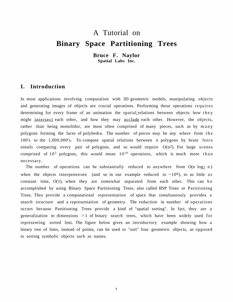
2

A Tutorial on

Binary Space Partitioning Trees

Bruce F. NaylorSpatial Labs Inc.

I. Introduction

In most applications involving computation with 3D geometric models, manipulating objects

and generating images of objects are crucial operations. Performing these operations r equ i r e s

determining for every frame of an animation the spatial relations between objects: how t h e y

might in tersect each other, and how they may occlude each other. However, the objects,

rather than being monolithic, are most often comprised of many pieces, such as by m a n y

polygons forming the faces of polyhedra. The number of pieces may be any where from t h e

100's to the 1,000,000's. To compute spatial relations between n polygons by brute force

entails comparing every pair of polygons, and so would require O(n2). For large scenes

comprised of 10 5 polygons, this would mean 1010 operations, which is much more t h a n

necessary.The number of operations can be substantially reduced to anywhere from O(n log2 n )

when the objects interpenetrate (and so in our example reduced to ~106), to as little a s

constant time, O(1), when they are somewhat separated from each other. This can b e

accomplished by using Binary Space Partitioning Trees, also called BSP Trees or Partitioning

Trees. They provide a computational representation of space that simultaneouly provides a

search structure and a representation of geometry. The reduction in number of operations

occurs because Partitioning Trees provide a kind of "spatial sorting". In fact, they are a

generalization to dimensions > 1 of binary search trees, which have been widely used for

representing sorted lists. The figure below gives an introductory example showing how a

binary tree of lines, instead of points, can be used to "sort" four geometric objects, as opposed

to sorting symbolic objects such as names.

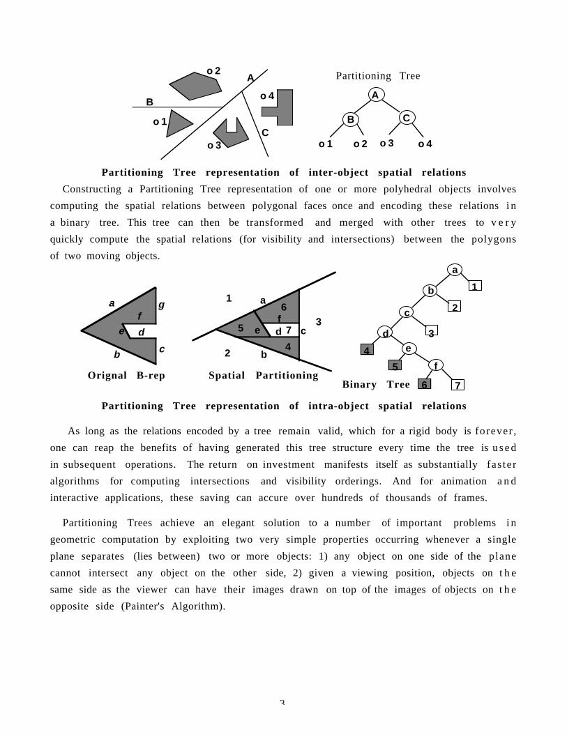
3

A

B

Co 1

o 2

o 3

o 4

o 3o 2o 1 o 4

Partitioning Tree

CB

A

Partitioning Tree representation of inter-object spatial relations

Constructing a Partitioning Tree representation of one or more polyhedral objects involves

computing the spatial relations between polygonal faces once and encoding these relations i n

a binary tree. This tree can then be transformed and merged with other trees to v e r y

quickly compute the spatial relations (for visibility and intersections) between the polygons

of two moving objects.a

b

c

de

f

1

2

3

7

4

5

6

a

b c

def

g

Orignal B-rep

a

b

cdef

1

2

3

4

5

6

7

Spatial PartitioningBinary Tree

Partitioning Tree representation of intra-object spatial relations

As long as the relations encoded by a tree remain valid, which for a rigid body is forever ,

one can reap the benefits of having generated this tree structure every time the tree is u s e d

in subsequent operations. The return on investment manifests itself as substantially fas ter

algorithms for computing intersections and visibility orderings. And for animation a n d

interactive applications, these saving can accure over hundreds of thousands of frames.

Partitioning Trees achieve an elegant solution to a number of important problems i n

geometric computation by exploiting two very simple properties occurring whenever a single

plane separates (lies between) two or more objects: 1) any object on one side of the plane

cannot intersect any object on the other side, 2) given a viewing position, objects on t h e

same side as the viewer can have their images drawn on top of the images of objects on t h e

opposite side (Painter's Algorithm).

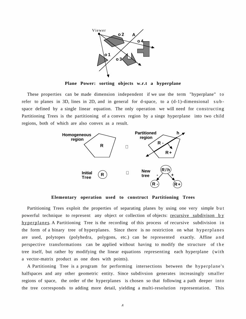
4

A

o 1

o 2

o 3

o 4

Viewer

Plane Power: sorting objects w.r.t a hyperplane

These properties can be made dimension independent if we use the term "hyperplane" t o

refer to planes in 3D, lines in 2D, and in general for d-space, to a (d-1)-dimensional s u b -

space defined by a single linear equation. The only operation we will need for constructing

Partitioning Trees is the partitioning of a convex region by a singe hyperplane into two child

regions, both of which are also convex as a result.

R -

R+

Initial Tree

Homogeneous region

Partitioned region

R

New treeR

⇒

⇒

h

R+R -

R / h- +

Elementary operation used to construct Partitioning Trees

Partitioning Trees exploit the properties of separating planes by using one very simple b u t

powerful technique to represent any object or collection of objects: recursive subdivison b y

hyperp lanes . A Partitioning Tree is the recording of this process of recursive subdivision i n

the form of a binary tree of hyperplanes. Since there is no restriction on what hyperp lanes

are used, polytopes (polyhedra, polygons, etc.) can be represented exactly. Affine a n d

perspective transformations can be applied without having to modify the structure of t h e

tree itself, but rather by modifying the linear equations representing each hyperplane (with

a vector-matrix product as one does with points).

A Partitioning Tree is a program for performing intersections between the hyperp lane ' s

halfspaces and any other geometric entity. Since subdivsion generates increasingly smaller

regions of space, the order of the hyperplanes is chosen so that following a path deeper into

the tree corresponds to adding more detail, yielding a multi-resolution representation. This

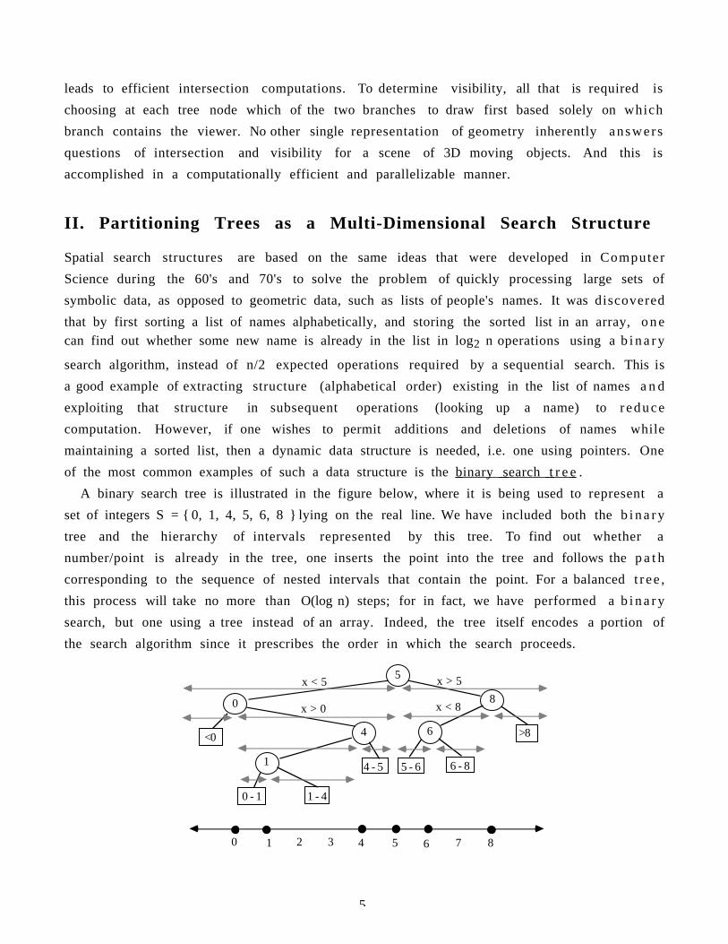
5

leads to efficient intersection computations. To determine visibility, all that is required is

choosing at each tree node which of the two branches to draw first based solely on which

branch contains the viewer. No other single representation of geometry inherently answers

questions of intersection and visibility for a scene of 3D moving objects. And this is

accomplished in a computationally efficient and parallelizable manner.

II. Partitioning Trees as a Multi-Dimensional Search Structure

Spatial search structures are based on the same ideas that were developed in Computer

Science during the 60's and 70's to solve the problem of quickly processing large sets of

symbolic data, as opposed to geometric data, such as lists of people's names. It was discovered

that by first sorting a list of names alphabetically, and storing the sorted list in an array, o n ecan find out whether some new name is already in the list in log2 n operations using a b i n a r y

search algorithm, instead of n/2 expected operations required by a sequential search. This is

a good example of extracting structure (alphabetical order) existing in the list of names a n d

exploiting that structure in subsequent operations (looking up a name) to r educe

computation. However, if one wishes to permit additions and deletions of names while

maintaining a sorted list, then a dynamic data structure is needed, i.e. one using pointers. One

of the most common examples of such a data structure is the binary search t r e e .

A binary search tree is illustrated in the figure below, where it is being used to represent a

set of integers S = 0, 1, 4, 5, 6, 8 lying on the real line. We have included both the b i n a r y

tree and the hierarchy of intervals represented by this tree. To find out whether a

number/point is already in the tree, one inserts the point into the tree and follows the p a t h

corresponding to the sequence of nested intervals that contain the point. For a balanced t r ee ,

this process will take no more than O(log n) steps; for in fact, we have performed a b i n a r y

search, but one using a tree instead of an array. Indeed, the tree itself encodes a portion of

the search algorithm since it prescribes the order in which the search proceeds.

0 1 2 3 4 5 6 7 8

5

0 8

64

1

<0

0 - 1 1 - 4

4 - 5 5 - 6 6 - 8

>8

x < 5 x > 5

x < 8x > 0

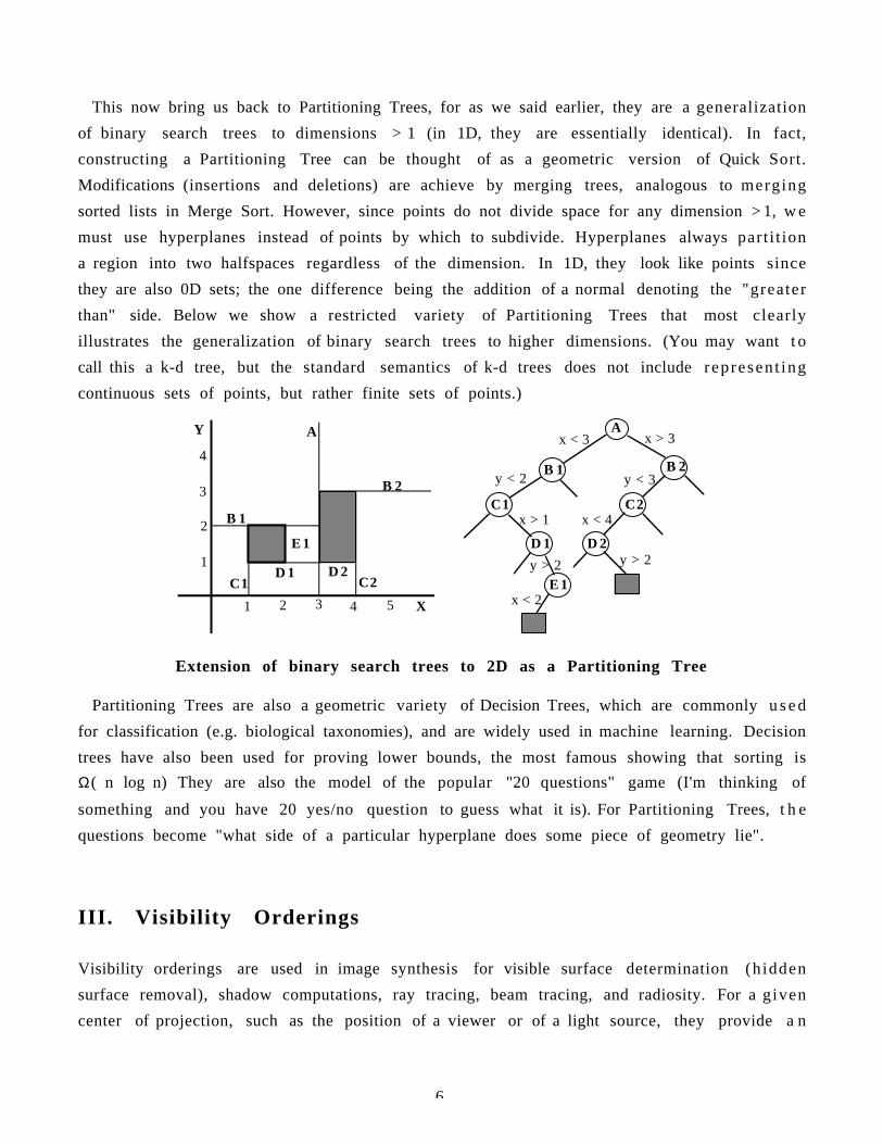
6

This now bring us back to Partitioning Trees, for as we said earlier, they are a generalization

of binary search trees to dimensions > 1 (in 1D, they are essentially identical). In fact,

constructing a Partitioning Tree can be thought of as a geometric version of Quick Sort.

Modifications (insertions and deletions) are achieve by merging trees, analogous to merging

sorted lists in Merge Sort. However, since points do not divide space for any dimension > 1, w e

must use hyperplanes instead of points by which to subdivide. Hyperplanes always part i t ion

a region into two halfspaces regardless of the dimension. In 1D, they look like points since

they are also 0D sets; the one difference being the addition of a normal denoting the "greater

than" side. Below we show a restricted variety of Partitioning Trees that most clearly

illustrates the generalization of binary search trees to higher dimensions. (You may want t o

call this a k-d tree, but the standard semantics of k-d trees does not include represen t ing

continuous sets of points, but rather finite sets of points.)

X

Y

31 2 4 5

1

2

3

4

A

B 2

B 1

C1 C2D 1 D 2

E 1

Ax < 3 x > 3

B 1 B 2

C2C1

D 1 D 2

y < 2 y < 3

x < 4x > 1

E 1y > 2

x < 2

y > 2

Extension of binary search trees to 2D as a Partitioning Tree

Partitioning Trees are also a geometric variety of Decision Trees, which are commonly u s e d

for classification (e.g. biological taxonomies), and are widely used in machine learning. Decision

trees have also been used for proving lower bounds, the most famous showing that sorting is

Ω( n log n) They are also the model of the popular "20 questions" game (I'm thinking of

something and you have 20 yes/no question to guess what it is). For Partitioning Trees, t h e

questions become "what side of a particular hyperplane does some piece of geometry lie".

III. Visibility Orderings

Visibility orderings are used in image synthesis for visible surface determination (hidden

surface removal), shadow computations, ray tracing, beam tracing, and radiosity. For a given

center of projection, such as the position of a viewer or of a light source, they provide a n

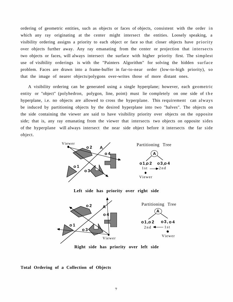
7

ordering of geometric entities, such as objects or faces of objects, consistent with the order i n

which any ray originating at the center might intersect the entities. Loosely speaking, a

visibility ordering assigns a priority to each object or face so that closer objects have pr ior i ty

over objects further away. Any ray emanating from the center or projection that intersects

two objects or faces, will always intersect the surface with higher priority first. The simplest

use of visibility orderings is with the "Painters Algorithm" for solving the hidden surface

problem. Faces are drawn into a frame-buffer in far-to-near order (low-to-high priority), so

that the image of nearer objects/polygons over-writes those of more distant ones.

A visibility ordering can be generated using a single hyperplane; however, each geometric

entity or "object" (polyhedron, polygon, line, point) must lie completely on one side of t h e

hyperplane, i.e. no objects are allowed to cross the hyperplane. This requirement can always

be induced by partitioning objects by the desired hyperplane into two "halves". The objects on

the side containing the viewer are said to have visibility priority over objects on the opposite

side; that is, any ray emanating from the viewer that intersects two objects on opposite sides

of the hyperplane will always intersect the near side object before it intersects the far side

object.

A

o 1

o 2

o 3

o 4

Viewer

o3 ,o 2o1 , o 4

Partitioning Tree

Viewer

1 s t 2 n d

A

Left side has priority over right side

A

o 1

o 2

o 3

o 4

Viewer

o3 ,o 2o1 , o 4

Partitioning Tree

Viewer

1 s t2 n d

A

Right side has priority over left side

Total Ordering of a Collection of Objects

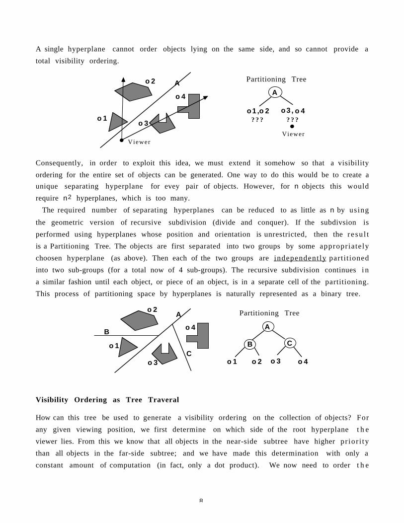
8

A single hyperplane cannot order objects lying on the same side, and so cannot provide a

total visibility ordering.

A

o 1

o 2

o 3

o 4

Viewer

A

o3 ,o 2o1 , o 4

Partitioning Tree

Viewer

? ? ? ? ? ?

Consequently, in order to exploit this idea, we must extend it somehow so that a visibility

ordering for the entire set of objects can be generated. One way to do this would be to create a

unique separating hyperplane for evey pair of objects. However, for n objects this would

require n2 hyperplanes, which is too many.

The required number of separating hyperplanes can be reduced to as little as n by using

the geometric version of recursive subdivision (divide and conquer). If the subdivsion is

performed using hyperplanes whose position and orientation is unrestricted, then the r e su l t

is a Partitioning Tree. The objects are first separated into two groups by some appropriately

choosen hyperplane (as above). Then each of the two groups are independent ly part i t ioned

into two sub-groups (for a total now of 4 sub-groups). The recursive subdivision continues i n

a similar fashion until each object, or piece of an object, is in a separate cell of the partitioning.

This process of partitioning space by hyperplanes is naturally represented as a binary tree.

A

B

Co 1

o 2

o 3

o 4

o 3o 2o 1 o 4

Partitioning Tree

CB

A

Visibility Ordering as Tree Traveral

How can this tree be used to generate a visibility ordering on the collection of objects? For

any given viewing position, we first determine on which side of the root hyperplane t h e

viewer lies. From this we know that all objects in the near-side subtree have higher pr ior i ty

than all objects in the far-side subtree; and we have made this determination with only a

constant amount of computation (in fact, only a dot product). We now need to order t h e

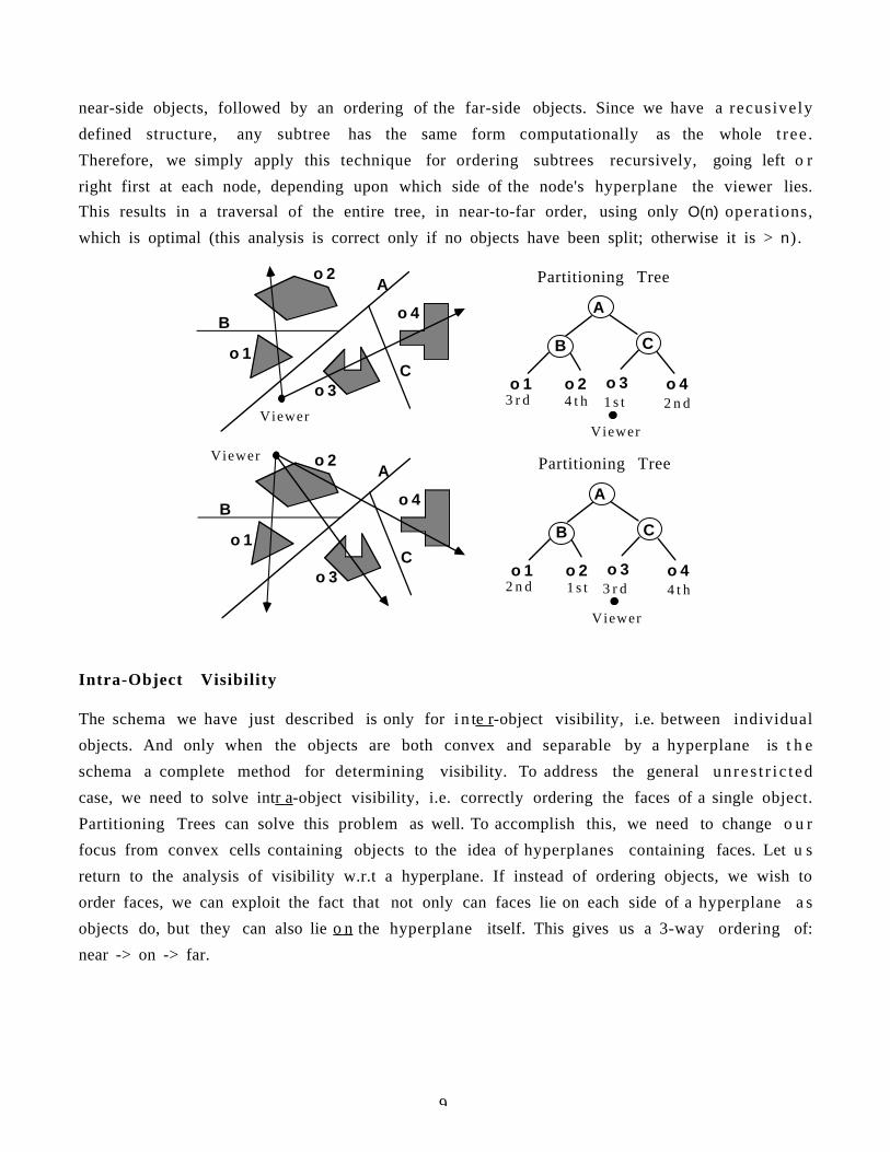
9

near-side objects, followed by an ordering of the far-side objects. Since we have a recusively

defined structure, any subtree has the same form computationally as the whole t ree .

Therefore, we simply apply this technique for ordering subtrees recursively, going left o r

right first at each node, depending upon which side of the node's hyperplane the viewer lies.

This results in a traversal of the entire tree, in near-to-far order, using only O(n) operations,

which is optimal (this analysis is correct only if no objects have been split; otherwise it is > n).

A

B

Co 1

o 2

o 3

o 4

Viewer

o 3o 2o 1 o 4

Viewer

3 r d 4 t h 1 s t 2 n d

Partitioning Tree

CB

A

A

B

Co 1

o 2

o 3

o 4

Viewer

o 3o 2o 1 o 4

Viewer

2 n d 1 s t 3 r d 4 t h

Partitioning Tree

CB

A

Intra-Object Visibility

The schema we have just described is only for i n t e r -object visibility, i.e. between individual

objects. And only when the objects are both convex and separable by a hyperplane is t h e

schema a complete method for determining visibility. To address the general unres t r i c ted

case, we need to solve int r a -object visibility, i.e. correctly ordering the faces of a single object.

Partitioning Trees can solve this problem as well. To accomplish this, we need to change o u r

focus from convex cells containing objects to the idea of hyperplanes containing faces. Let u s

return to the analysis of visibility w.r.t a hyperplane. If instead of ordering objects, we wish to

order faces, we can exploit the fact that not only can faces lie on each side of a hyperplane a s

objects do, but they can also lie o n the hyperplane itself. This gives us a 3-way ordering of:

near -> on -> far.

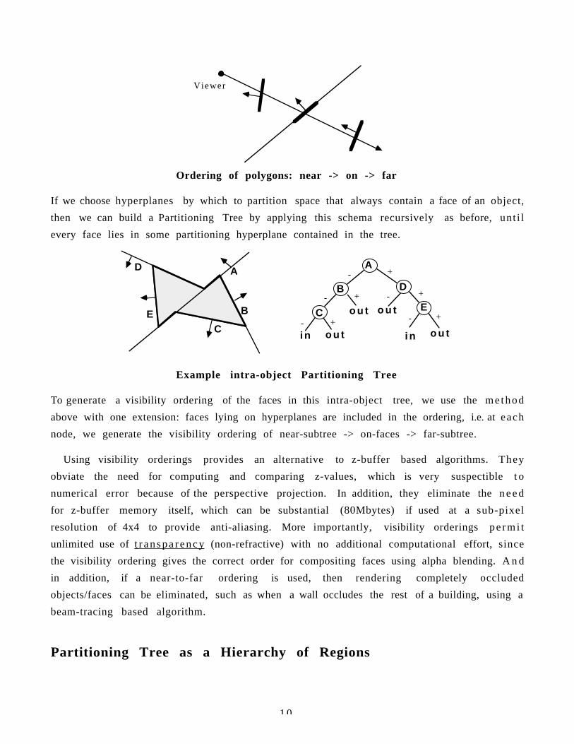
1 0

Viewer

Ordering of polygons: near -> on -> far

If we choose hyperplanes by which to partition space that always contain a face of an object,

then we can build a Partitioning Tree by applying this schema recursively as before, unt i l

every face lies in some partitioning hyperplane contained in the tree.

A

B

C

D

E o u t

i n o u t o u ti n

o u t

A

B

C

D

E

- +

- + - +

- + - +

Example intra-object Partitioning Tree

To generate a visibility ordering of the faces in this intra-object tree, we use the me thod

above with one extension: faces lying on hyperplanes are included in the ordering, i.e. at each

node, we generate the visibility ordering of near-subtree -> on-faces -> far-subtree.

Using visibility orderings provides an alternative to z-buffer based algorithms. They

obviate the need for computing and comparing z-values, which is very suspectible t o

numerical error because of the perspective projection. In addition, they eliminate the n e e d

for z-buffer memory itself, which can be substantial (80Mbytes) if used at a sub-pixel

resolution of 4x4 to provide anti-aliasing. More importantly, visibility orderings pe rmi t

unlimited use of t r a n s p a r e n c y (non-refractive) with no additional computational effort, since

the visibility ordering gives the correct order for compositing faces using alpha blending. A n d

in addition, if a near-to-far ordering is used, then rendering completely occluded

objects/faces can be eliminated, such as when a wall occludes the rest of a building, using a

beam-tracing based algorithm.

Partitioning Tree as a Hierarchy of Regions

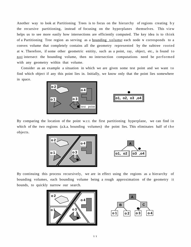
1 1

Another way to look at Partitioning Trees is to focus on the hierarchy of regions creating b y

the recursive partitioning, instead of focusing on the hyperplanes themselves. This view

helps us to see more easily how intersections are efficiently computed. The key idea is to th ink

of a Partitioning Tree region as serving as a bounding vo lume : each node v corresponds to a

convex volume that completely contains all the geometry represented by the subtree rooted

at v . Therefore, if some other geometric enitity, such as a point, ray, object, etc., is found t o

n o t intersect the bounding volume, then no intersection computations need be per formed

with any geometry within that volume.

Consider as an example a situation in which we are given some test point and we want t o

find which object if any this point lies in. Initially, we know only that the point lies somewhere

in space.

o1, o2, o3 ,o4o 1

o 2

o 3

o 4

test point

By comparing the location of the point w.r.t. the first partitioning hyperplane, we can find i n

which of the two regions (a.k.a. bounding volumes) the point lies. This eliminates half of t h e

objects.

A

o1, o2 o3 ,o4o 1

o 2

o 3

o 4

By continuing this process recursively, we are in effect using the regions as a hierarchy of

bounding volumes, each bounding volume being a rough approximation of the geometry i t

bounds, to quickly narrow our search.

A

B C

o 1 o 2 o 3 o 4o 1

o 2

o 3

o 4

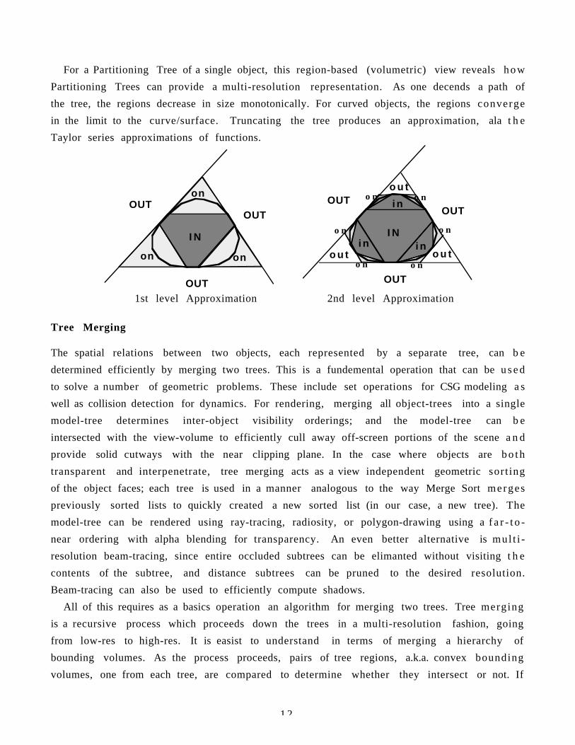
1 2

For a Partitioning Tree of a single object, this region-based (volumetric) view reveals how

Partitioning Trees can provide a multi-resolution representation. As one decends a path of

the tree, the regions decrease in size monotonically. For curved objects, the regions converge

in the limit to the curve/surface. Truncating the tree produces an approximation, ala t h e

Taylor series approximations of functions.

I N

OUTOUT

OUT

on on

on

1st level Approximation

I N

OUTOUT

OUT

o u t

o u t

o u ti ni n

i n

2nd level Approximation

o n

o n

o n o n

o n

o n

Tree Merging

The spatial relations between two objects, each represented by a separate tree, can b e

determined efficiently by merging two trees. This is a fundemental operation that can be u s e d

to solve a number of geometric problems. These include set operations for CSG modeling a s

well as collision detection for dynamics. For rendering, merging all object-trees into a single

model-tree determines inter-object visibility orderings; and the model-tree can b e

intersected with the view-volume to efficiently cull away off-screen portions of the scene a n d

provide solid cutways with the near clipping plane. In the case where objects are b o t h

transparent and interpenetrate, tree merging acts as a view independent geometric sort ing

of the object faces; each tree is used in a manner analogous to the way Merge Sort merges

previously sorted lists to quickly created a new sorted list (in our case, a new tree). The

model-tree can be rendered using ray-tracing, radiosity, or polygon-drawing using a f a r - t o -

near ordering with alpha blending for transparency. An even better alternative is mul t i -

resolution beam-tracing, since entire occluded subtrees can be elimanted without visiting t h e

contents of the subtree, and distance subtrees can be pruned to the desired resolution.

Beam-tracing can also be used to efficiently compute shadows.

All of this requires as a basics operation an algorithm for merging two trees. Tree merging

is a recursive process which proceeds down the trees in a multi-resolution fashion, going

from low-res to high-res. It is easist to understand in terms of merging a hierarchy of

bounding volumes. As the process proceeds, pairs of tree regions, a.k.a. convex bounding

volumes, one from each tree, are compared to determine whether they intersect or not. If

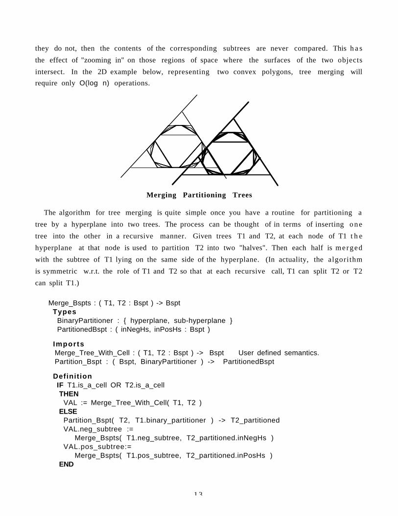
1 3

they do not, then the contents of the corresponding subtrees are never compared. This h a s

the effect of "zooming in" on those regions of space where the surfaces of the two objects

intersect. In the 2D example below, representing two convex polygons, tree merging will

require only O(log n) operations.

Merging Partitioning Trees

The algorithm for tree merging is quite simple once you have a routine for partitioning a

tree by a hyperplane into two trees. The process can be thought of in terms of inserting o n e

tree into the other in a recursive manner. Given trees T1 and T2, at each node of T1 t h e

hyperplane at that node is used to partition T2 into two "halves". Then each half is merged

with the subtree of T1 lying on the same side of the hyperplane. (In actuality, the algorithm

is symmetric w.r.t. the role of T1 and T2 so that at each recursive call, T1 can split T2 or T2

can split T1.)

Merge_Bspts : ( T1, T2 : Bspt ) -> Bspt Types

BinaryPartitioner : hyperplane, sub-hyperplane PartitionedBspt : ( inNegHs, inPosHs : Bspt )

ImportsMerge_Tree_With_Cell : ( T1, T2 : Bspt ) -> Bspt User defined semantics.Partition_Bspt : ( Bspt, BinaryPartitioner ) -> PartitionedBspt

Definition IF T1.is_a_cell OR T2.is_a_cell THEN

VAL := Merge_Tree_With_Cell( T1, T2 ) ELSE

Partition_Bspt( T2, T1.binary_partitioner ) -> T2_partitionedVAL.neg_subtree :=

Merge_Bspts( T1.neg_subtree, T2_partitioned.inNegHs )VAL.pos_subtree:=

Merge_Bspts( T1.pos_subtree, T2_partitioned.inPosHs ) END

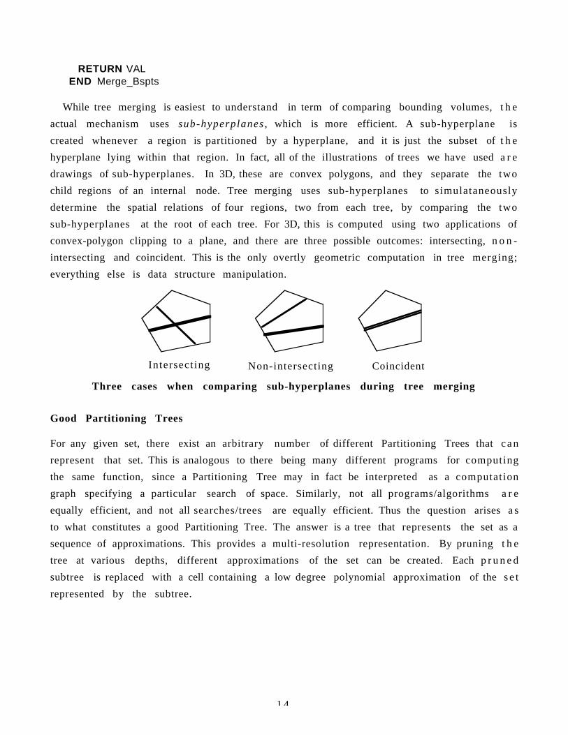
1 4

RETURN VALEND Merge_Bspts

While tree merging is easiest to understand in term of comparing bounding volumes, t h e

actual mechanism uses sub-hyperplanes , which is more efficient. A sub-hyperplane is

created whenever a region is partitioned by a hyperplane, and it is just the subset of t h e

hyperplane lying within that region. In fact, all of the illustrations of trees we have used a r e

drawings of sub-hyperplanes. In 3D, these are convex polygons, and they separate the two

child regions of an internal node. Tree merging uses sub-hyperplanes to simulataneously

determine the spatial relations of four regions, two from each tree, by comparing the two

sub-hyperplanes at the root of each tree. For 3D, this is computed using two applications of

convex-polygon clipping to a plane, and there are three possible outcomes: intersecting, n o n -

intersecting and coincident. This is the only overtly geometric computation in tree merging;

everything else is data structure manipulation.

Intersect ing CoincidentNon-intersecting

Three cases when comparing sub-hyperplanes during tree merging

Good Partitioning Trees

For any given set, there exist an arbitrary number of different Partitioning Trees that c a n

represent that set. This is analogous to there being many different programs for computing

the same function, since a Partitioning Tree may in fact be interpreted as a computation

graph specifying a particular search of space. Similarly, not all programs/algorithms a r e

equally efficient, and not all searches/trees are equally efficient. Thus the question arises a s

to what constitutes a good Partitioning Tree. The answer is a tree that represents the set as a

sequence of approximations. This provides a multi-resolution representation. By pruning t h e

tree at various depths, different approximations of the set can be created. Each p r u n e d

subtree is replaced with a cell containing a low degree polynomial approximation of the s e t

represented by the subtree.

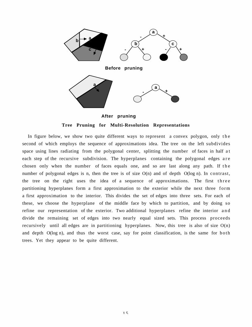
1 5

ab

c

a

b c

+

++

-

- -

aa

+-

Before pruning

After pruning

Tree Pruning for Multi-Resolution Representations

In figure below, we show two quite different ways to represent a convex polygon, only t h e

second of which employs the sequence of approximations idea. The tree on the left subdivides

space using lines radiating from the polygonal center, splitting the number of faces in half a t

each step of the recursive subdivision. The hyperplanes containing the polygonal edges a r e

chosen only when the number of faces equals one, and so are last along any path. If t h e

number of polygonal edges is n, then the tree is of size O(n) and of depth O(log n). In contrast ,

the tree on the right uses the idea of a sequence of approximations. The first t h r e e

partitioning hyperplanes form a first approximation to the exterior while the next three fo rm

a first approximation to the interior. This divides the set of edges into three sets. For each of

these, we choose the hyperplane of the middle face by which to partition, and by doing so

refine our representation of the exterior. Two additional hyperplanes refine the interior a n d

divide the remaining set of edges into two nearly equal sized sets. This process proceeds

recursively until all edges are in partitioning hyperplanes. Now, this tree is also of size O(n)

and depth O(log n), and thus the worst case, say for point classification, is the same for b o t h

trees. Yet they appear to be quite different.

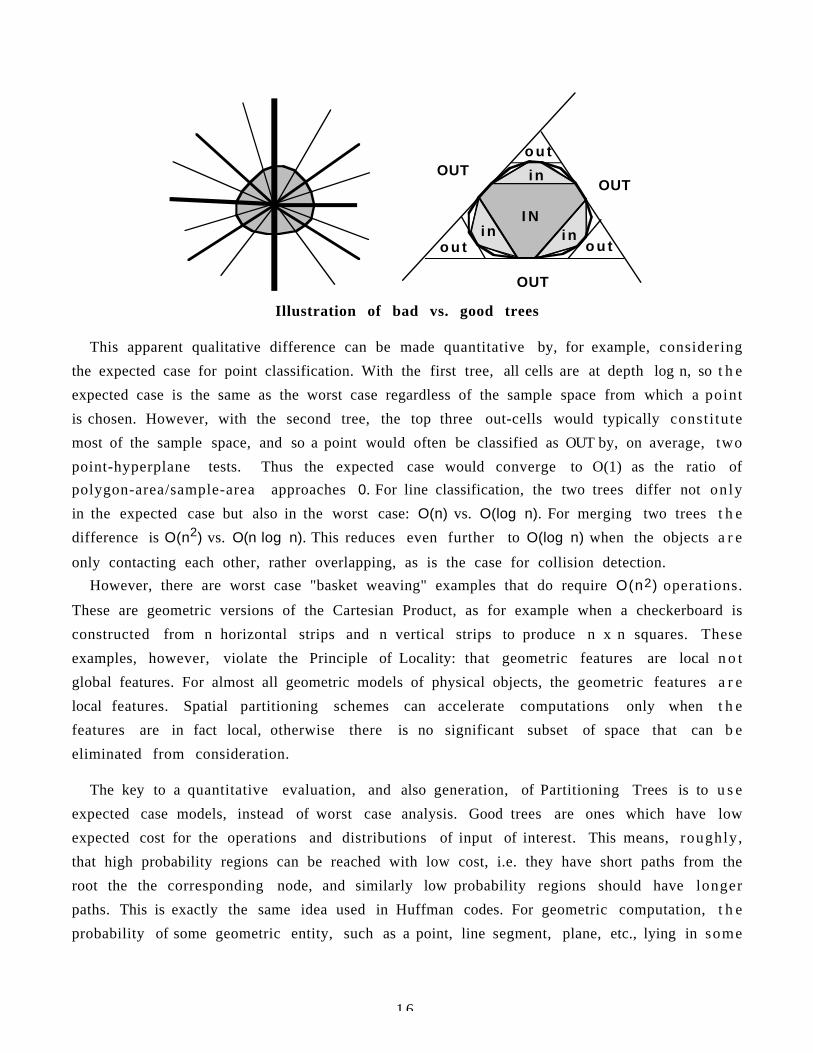
1 6

I N

OUTOUT

OUT

o u t

o u t

o u ti ni n

i n

Illustration of bad vs. good trees

This apparent qualitative difference can be made quantitative by, for example, considering

the expected case for point classification. With the first tree, all cells are at depth log n, so t h e

expected case is the same as the worst case regardless of the sample space from which a point

is chosen. However, with the second tree, the top three out-cells would typically consti tute

most of the sample space, and so a point would often be classified as OUT by, on average, two

point-hyperplane tests. Thus the expected case would converge to O(1) as the ratio of

polygon-area/sample-area approaches 0. For line classification, the two trees differ not only

in the expected case but also in the worst case: O(n) vs. O(log n). For merging two trees t h e

difference is O(n2) vs. O(n log n). This reduces even further to O(log n) when the objects a r e

only contacting each other, rather overlapping, as is the case for collision detection.

However, there are worst case "basket weaving" examples that do require O(n2) operations.

These are geometric versions of the Cartesian Product, as for example when a checkerboard is

constructed from n horizontal strips and n vertical strips to produce n x n squares. These

examples, however, violate the Principle of Locality: that geometric features are local n o t

global features. For almost all geometric models of physical objects, the geometric features a r e

local features. Spatial partitioning schemes can accelerate computations only when t h e

features are in fact local, otherwise there is no significant subset of space that can b e

eliminated from consideration.

The key to a quantitative evaluation, and also generation, of Partitioning Trees is to u s e

expected case models, instead of worst case analysis. Good trees are ones which have low

expected cost for the operations and distributions of input of interest. This means, roughly,

that high probability regions can be reached with low cost, i.e. they have short paths from the

root the the corresponding node, and similarly low probability regions should have longer

paths. This is exactly the same idea used in Huffman codes. For geometric computation, t h e

probability of some geometric entity, such as a point, line segment, plane, etc., lying in some

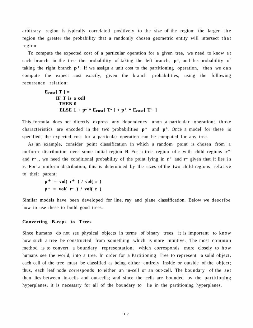
1 7

arbitrary region is typically correlated positively to the size of the region: the larger t h e

region the greater the probability that a randomly chosen geometric entity will intersect t h a t

region.

To compute the expected cost of a particular operation for a given tree, we need to know a t

each branch in the tree the probability of taking the left branch, p - , and he probability of

taking the right branch p+ . If we assign a unit cost to the partitioning operation, then we c a n

compute the expect cost exactly, given the branch probabilities, using the following

recurrence relation:

Ecost[ T ] =IF T is a cell THEN 0 ELSE 1 + p- * Ecost[ T- ] + p+ * Ecost[ T+ ]

This formula does not directly express any dependency upon a particular operation; those

characteristics are encoded in the two probabilities p - and p+. Once a model for these is

specified, the expected cost for a particular operation can be computed for any tree.

As an example, consider point classification in which a random point is chosen from a

uniform distribution over some initial region R. For a tree region of r with child regions r+

and r- , we need the conditional probability of the point lying in r+ and r- given that it lies i n

r . For a uniform distribution, this is determined by the sizes of the two child-regions relat ive

to their parent:

p + = vol( r+ ) / vol( r )

p - = vol( r- ) / vol( r )

Similar models have been developed for line, ray and plane classification. Below we describe

how to use these to build good trees.

Converting B-reps to Trees

Since humans do not see physical objects in terms of binary trees, it is important to know

how such a tree be constructed from something which is more intuitive. The most common

method is to convert a boundary representation, which corresponds more closely to how

humans see the world, into a tree. In order for a Partitioning Tree to represent a solid object,

each cell of the tree must be classified as being either entirely inside or outside of the object;

thus, each leaf node corresponds to either an in-cell or an out-cell. The boundary of the s e t

then lies between in-cells and out-cells; and since the cells are bounded by the partitioning

hyperplanes, it is necessary for all of the boundary to lie in the partitioning hyperplanes.

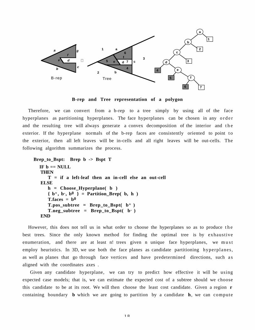
1 8

a

b c

de

fg

a

b

c

d

e

f

1

2

3

7

4

5

6

a

b

cdef

1

2

3

4

5

6

7⇒

B-rep Tree

B-rep and Tree representation of a polygon

Therefore, we can convert from a b-rep to a tree simply by using all of the face

hyperplanes as partitioning hyperplanes. The face hyperplanes can be chosen in any o r d e r

and the resulting tree will always generate a convex decomposition of the interior and t h e

exterior. If the hyperplane normals of the b-rep faces are consistently oriented to point t o

the exterior, then all left leaves will be in-cells and all right leaves will be out-cells. The

following algorithm summarizes the process.

Brep_to_Bspt: Brep b -> Bspt T

IF b == NULL THEN

T = if a left-leaf then an in-cell else an out-cell ELSE

h = Choose_Hyperplane( b ) b+ , b-, b0 = Partition_Brep( b, h )T.faces = b0

T.pos_subtree = Brep_to_Bspt( b+ )T.neg_subtree = Brep_to_Bspt( b- )

END

However, this does not tell us in what order to choose the hyperplanes so as to produce t h e

best trees. Since the only known method for finding the optimal tree is by exhaust ive

enumeration, and there are at least n! trees given n unique face hyperplanes, we m u s t

employ heuristics. In 3D, we use both the face planes as candidate partitioning hyperplanes ,

as well as planes that go through face vertices and have predetermined directions, such a s

aligned with the coordinates axes .

Given any candidate hyperplane, we can try to predict how effective it will be using

expected case models; that is, we can estimate the expected cost of a subtree should we choose

this candidate to be at its root. We will then choose the least cost candidate. Given a region r

containing boundary b which we are going to partition by a candidate h , we can compute

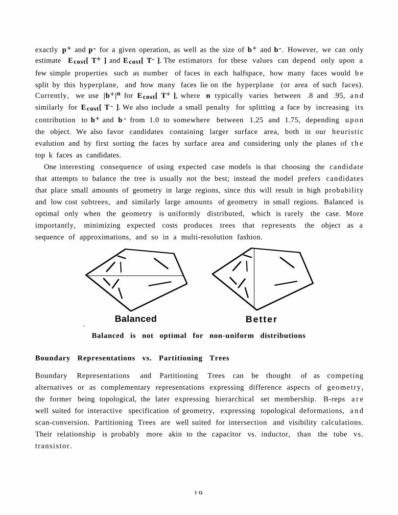
1 9

exactly p+ and p- for a given operation, as well as the size of b+ and b-. However, we can only

estimate Ecost[ T+ ] and Ecost[ T- ]. The estimators for these values can depend only upon a

few simple properties such as number of faces in each halfspace, how many faces would b e

split by this hyperplane, and how many faces lie on the hyperplane (or area of such faces).

Currently, we use |b+|n for Ecost[ T+ ], where n typically varies between .8 and .95, a n d

similarly for Ecost[ T - ]. We also include a small penalty for splitting a face by increasing its

contribution to b+ and b - from 1.0 to somewhere between 1.25 and 1.75, depending u p o n

the object. We also favor candidates containing larger surface area, both in our heurist ic

evalution and by first sorting the faces by surface area and considering only the planes of t h e

top k faces as candidates.

One interesting consequence of using expected case models is that choosing the candidate

that attempts to balance the tree is usually not the best; instead the model prefers candidates

that place small amounts of geometry in large regions, since this will result in high probability

and low cost subtrees, and similarly large amounts of geometry in small regions. Balanced is

optimal only when the geometry is uniformly distributed, which is rarely the case. More

importantly, minimizing expected costs produces trees that represents the object as a

sequence of approximations, and so in a multi-resolution fashion.

.Balanced Better

Balanced is not optimal for non-uniform distributions

Boundary Representations vs. Partitioning Trees

Boundary Representations and Partitioning Trees can be thought of as competing

alternatives or as complementary representations expressing difference aspects of geometry ,

the former being topological, the later expressing hierarchical set membership. B-reps a r e

well suited for interactive specification of geometry, expressing topological deformations, a n d

scan-conversion. Partitioning Trees are well suited for intersection and visibility calculations.

Their relationship is probably more akin to the capacitor vs. inductor, than the tube vs.

t ransistor .

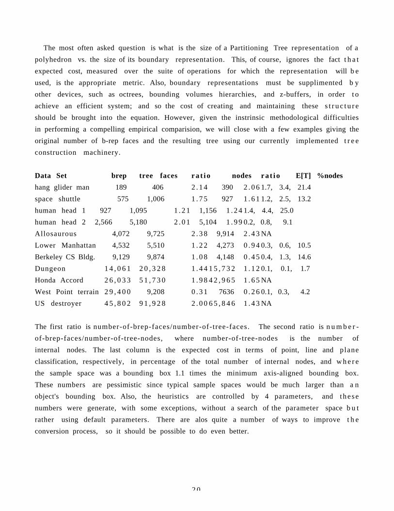
2 0

The most often asked question is what is the size of a Partitioning Tree representation of a

polyhedron vs. the size of its boundary representation. This, of course, ignores the fact t h a t

expected cost, measured over the suite of operations for which the representation will b e

used, is the appropriate metric. Also, boundary representations must be supplimented b y

other devices, such as octrees, bounding volumes hierarchies, and z-buffers, in order t o

achieve an efficient system; and so the cost of creating and maintaining these s t r u c t u r e

should be brought into the equation. However, given the instrinsic methodological difficulties

in performing a compelling empirical comparision, we will close with a few examples giving the

original number of b-rep faces and the resulting tree using our currently implemented t r e e

construction machinery.

Data Set brep tree faces r a t i o nodes r a t i o E[T] %nodes

hang glider man 189 406 2 . 1 4 390 2 . 0 6 1.7, 3.4, 21.4

space shuttle 575 1,006 1 . 7 5 927 1 . 6 1 1.2, 2.5, 13.2

human head 1 927 1,095 1 . 2 1 1,156 1 . 2 4 1.4, 4.4, 25.0

human head 2 2,566 5,180 2 . 0 1 5,104 1 . 9 9 0.2, 0.8, 9.1

Allosaurous 4,072 9,725 2 . 3 8 9,914 2 . 4 3 NA

Lower Manhattan 4,532 5,510 1 . 2 2 4,273 0 . 9 4 0.3, 0.6, 10.5

Berkeley CS Bldg. 9,129 9,874 1 . 0 8 4,148 0 . 4 5 0.4, 1.3, 14.6

Dungeon 1 4 , 0 6 1 2 0 , 3 2 8 1 . 4 4 1 5 , 7 3 2 1 . 1 2 0.1, 0.1, 1.7

Honda Accord 2 6 , 0 3 3 5 1 , 7 3 0 1 . 9 8 4 2 , 9 6 5 1 . 6 5 NA

West Point terrain 2 9 , 4 0 0 9,208 0 . 3 1 7636 0 . 2 6 0.1, 0.3, 4.2

US destroyer 4 5 , 8 0 2 9 1 , 9 2 8 2 . 0 0 6 5 , 8 4 6 1 . 4 3 NA

The first ratio is number-of-brep-faces/number-of-tree-faces. The second ratio is n u m b e r -

of-brep-faces/number-of-tree-nodes, where number-of-tree-nodes is the number of

internal nodes. The last column is the expected cost in terms of point, line and plane

classification, respectively, in percentage of the total number of internal nodes, and w h e r e

the sample space was a bounding box 1.1 times the minimum axis-aligned bounding box.

These numbers are pessimistic since typical sample spaces would be much larger than a n

object's bounding box. Also, the heuristics are controlled by 4 parameters, and t h e s e

numbers were generate, with some exceptions, without a search of the parameter space b u t

rather using default parameters. There are alos quite a number of ways to improve t h e

conversion process, so it should be possible to do even better.

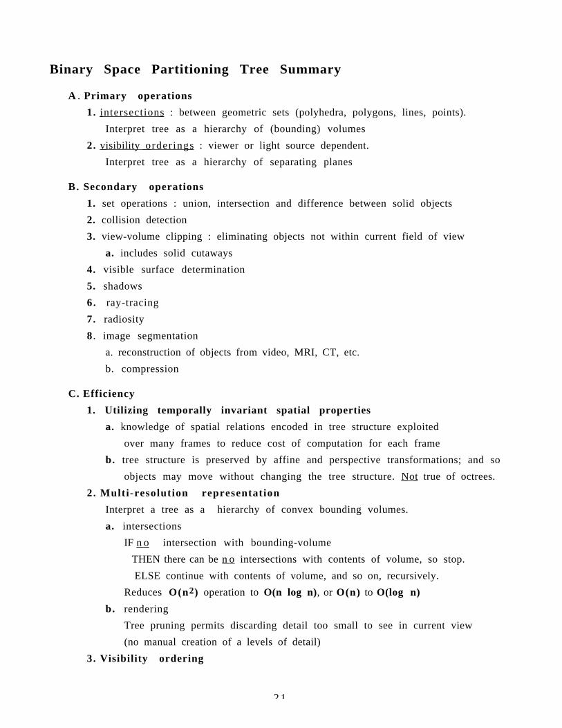
2 1

Binary Space Partitioning Tree Summary

A . Primary operations

1. intersections : between geometric sets (polyhedra, polygons, lines, points).

Interpret tree as a hierarchy of (bounding) volumes

2. visibility order ings : viewer or light source dependent.

Interpret tree as a hierarchy of separating planes

B. Secondary operations

1. set operations : union, intersection and difference between solid objects

2. collision detection

3. view-volume clipping : eliminating objects not within current field of view

a. includes solid cutaways

4. visible surface determination

5. shadows

6. ray-tracing

7. radiosity

8 . image segmentation

a. reconstruction of objects from video, MRI, CT, etc.

b. compression

C. Efficiency

1. Utilizing temporally invariant spatial properties

a. knowledge of spatial relations encoded in tree structure exploited

over many frames to reduce cost of computation for each frame

b. tree structure is preserved by affine and perspective transformations; and so

objects may move without changing the tree structure. Not true of octrees.

2. Multi-resolution representation

Interpret a tree as a hierarchy of convex bounding volumes.

a. intersections

IF n o intersection with bounding-volume

THEN there can be n o intersections with contents of volume, so stop.

ELSE continue with contents of volume, and so on, recursively.

Reduces O(n2) operation to O(n log n), or O(n) to O(log n)

b. rendering

Tree pruning permits discarding detail too small to see in current view

(no manual creation of a levels of detail)

3. Visibility ordering

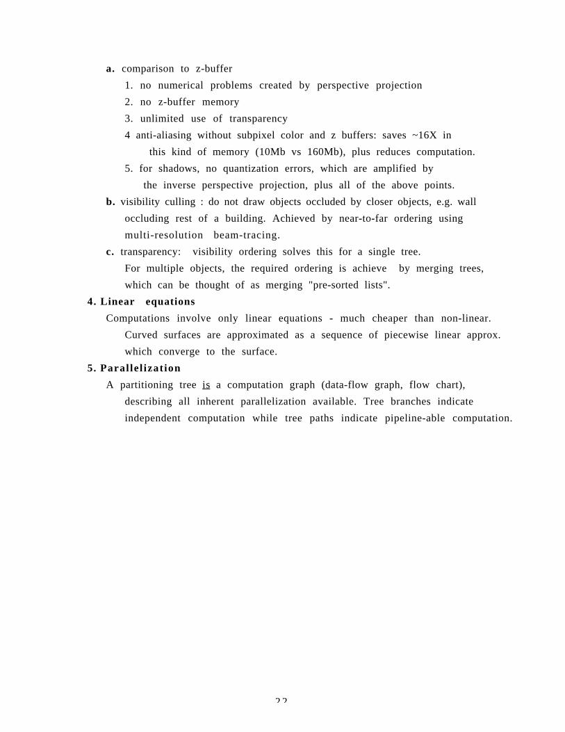
2 2

a. comparison to z-buffer

1. no numerical problems created by perspective projection

2. no z-buffer memory

3. unlimited use of transparency

4 anti-aliasing without subpixel color and z buffers: saves ~16X in

this kind of memory (10Mb vs 160Mb), plus reduces computation.

5. for shadows, no quantization errors, which are amplified by

the inverse perspective projection, plus all of the above points.

b. visibility culling : do not draw objects occluded by closer objects, e.g. wall

occluding rest of a building. Achieved by near-to-far ordering using

multi-resolution beam-tracing.

c. transparency: visibility ordering solves this for a single tree.

For multiple objects, the required ordering is achieve by merging trees,

which can be thought of as merging "pre-sorted lists".

4. Linear equations

Computations involve only linear equations - much cheaper than non-linear.

Curved surfaces are approximated as a sequence of piecewise linear approx.

which converge to the surface.

5. Parallel ization

A partitioning tree is a computation graph (data-flow graph, flow chart),

describing all inherent parallelization available. Tree branches indicate

independent computation while tree paths indicate pipeline-able computation.

2 3

Bibliography (partial)

Solid Modeling

[Bloomberg 86]

Sandra H. Bloomberg, "A Representation of Solid Objects for Performing Boolean

Operations", U.N.C. Computer Science Technical Report 86-006 (1986).

[Thibault and Naylor 87]

W. Thibault and B. Naylor, "Set Operations On Polyhedra Using Binary Space Partitioning

Trees", Computer Graphics Vol. 21(4), pp. 153-162, (July 1987).

[Naylor, Amanatides and Thibault 90]

Bruce F. Naylor, John Amanatides and William C. Thibault, "Merging BSP Trees Yields

Polyhedral Set Operations", Computer Graphics Vol. 24(4), pp. 115-124, (Augus t

1 9 9 0 ) .

[Naylor 90a]

Bruce F. Naylor, "Binary Space Partitioning Trees as an Alternative Representation of

Polytopes," Computer Aided Design, Vol. 22(4), (May 1990).

[Naylor 90b]

Bruce F. Naylor, "SCULPT: an Interactive Solid Modeling Tool," Proceeding of Graphics

Interface (May 1990).

[Torres 90]

Enric Torres, "Optimization of the Binary Space Partition Algorithm (BSP) for t h e

Visualization of Dynamic Scenes" Eurographics ‘90 (Sept. 1990).

[Ihm and Naylor 91]

Insung Ihm and Bruce Naylor, "Piecewise Linear Approximations of Curves wi th

Applications," Proceeding of Computer Graphics International '91, Springer-Verlag

(June 1991).

[Naylor 92a]

Bruce F. Naylor, "Interactive Solid Modeling Via Partitioning Trees", Proceeding of

Graphics Interface , pp 11-18, (May 1992).

[Chrysanthou and Slater 92]

Y. Chrysanthou and M. Slater, "Computing Dynamic Changes to BSP Trees", Eurographics

‘92, 11(3), pp. 321-332.

2 4

Visibi l i ty

[Schumacker et al 69]

R. A. Schumacker, R. Brand, M. Gilliland, and W. Sharp, "Study for Applying Compute r -

Generated Images to Visual Simulation," AFHRL-TR-69-14, U.S. Air Force Human

Resources Laboratory (1969).

[Ivan Sutherland 73]

Ivan E. Sutherland, "Polygon Sorting by Subdivision: a Solution to the Hidden-Surface

Problem", unpublished manuscript, (October 1973).

[Fuchs, Kedem, and Naylor 80]

H. Fuchs, Z. Kedem, and B. Naylor, "On Visible Surface Generation by a Priori Tree

Structures," Computer Graphics Vol. 14(3), pp. 124-133, (June 1980).

[Fuchs, Abrams, and Grant 83]

Henry Fuchs, Gregory Abrams and Eric Grant, "Near Real-Time Shaded Display of Rigid

Objects", Computer Graphics Vol. 17(3), pp. 65-72, (July 1983).

[Naylor and Thibault 86]

Bruce F. Naylor and William C. Thibault, "Application of BSP Trees to Ray-Tracing a n d

CSG Evaluation", Technical Report GIT-ICS 86/03, School of Information and Computer

Science, Georgia Institute of Technology, Atlanta, Georgia 30332 (February 1986).

[Chin and Feiner 89]

Norman Chin and Steve Feiner, "Near Real-Time Shadow Generation Using BSP Trees",

Computer Graphics Vol. 23(3), pp. 99-106, (July 1989).

[Campbell and Fussell 90]

A.T. Campbell and Donald S. Fussell, "Adaptive Mesh Generation for Global Diffuse

Illumination", Computer Graphics Vol. 24(4), pp. 155-164, (August 1990).

[Campbell 91]

A.T. Campbell "Modeling Global Diffuse for Image Synthesis", Ph.D. Dissertation,

Department of Computer Science, University of Texas at Austin, (1991).

[Gordon and Chen 91]

Dan Gordon and Shuhong Chen, "Front-to-Back Display of BSP Trees", IEEE Computer

Graphics & Applications, pp. 79-85, (September 1991).

[Chin and Feiner 92]

2 5

Norman Chin and Steve Feiner, "Fast Object-Precision Shadow Generation for Area Light

Sources Using BSP Trees", Symp. on 3D Interactive Graphics, (March 1992).

[Naylor 92a]

Bruce F. Naylor, "Partitioning Tree Image Representation and Generation from 3D

Geometric Models", Proceeding of Graphics Interface (May 1992).

[Lischinski, Tampieri and Greenburg 92]

Dani Lischinski, Filippo Tampieri and Donald Greenburg, "Discountinuity Meshing for

Accurate Radiosity", IEEE Computer Graphics & Applications 12(6), pp. 2 5 - 3 9 ,

(November 1992).

[Teller and Hanrahan 93]

Seth Teller and Pat Hanrahan, "Global Visibility Algorithms for Illumination

Computations", Computer Graphics Vol. 27, pp. 239-246, (August 1993).

Image Representation

[Rahda et al 91]

Hayder Rahda, Riccardo Leonardi, Martin Vetterli and Bruce Naylor, "Binary Space

Partitioning Tree Representation of Images", Visual Communications and I m a g e

Representation , Vol. 2(3), pp. 201-221, ( Sept. 1991).

[Subramanian and Naylor 92]

K.R. Subramanian and Bruce Naylor, "Representing Medical images with Partitioning

Trees", Proceeding of Visualization '92, (Oct. 1992).

[Radha 93]

Hayder M. Sadik Radha, "Efficient Image Representation Using Binary Space Partitioning

Trees", Ph.D. dissertation, CU/CTR/TR 343-93-23, Columbia University, (1993).

T h e o r y

[Rabin 72]

Michael O. Rabin, "Proving Simultaneous Positivity of Linear Forms", Journal o f

Computer and Systems Science, v6, pp. 639-650 (1991).

[Reingold 72]

E. M. Reingold, "On the Optimality of some Set Operations", Journal of the ACM, Vol. 1 9 ,

pp. 649-659 (1972).

[Naylor 81]

2 6

Bruce F. Naylor, "A Priori Based Techniques for Determining Visibility Priority for 3 -D

Scenes," Ph.D. Thesis, University of Texas at Dallas (May 1981).

[Paterson and Yao 90]

M.S. Paterson and F.F. Yao, "Efficient Binary Space Partitions for Hidden-Surface Removal

and Solid Modeling", Discrete & Computational Geometry, v5, pp. 485-503, 1990.

[Paterson and Yao 92]

M.S. Paterson and F.F. Yao, "Optimal Binary Space Partitions for Orthogonal Objects",

Journal of Algorithms, v5, pp. 99-113, 1992.

[Naylor 93]

Bruce F. Naylor, "Constructing Good Partitioning Trees", Graphics Interface '93, Toronto

CA, pp. 181-191, (May 1993).

[Berg, Groot and Overmars 93]

MMark de Berg, Marko M. de Groot and Mark Overmars, "Perfect Binary Space Partitions",

Canadian Conference on Computational Geometry, 1993.