review of basic concepts - bgu courses/appa...503 a ppendix a review of basic concepts objectives...

503

A P P E N D I X A

Review Of Basic Concepts

Objectives

The objective of this appendix is to review the basic concepts usually covered in an under-graduate course in process control. Concepts reviewed include:

• Block diagram representation of control systems. • Laplace transform and transfer functions. • Analysis of block diagrams. • P, PI, and PID controllers. • Stability of feedback control systems.

504 Review Of Basic Concepts Appendix A

A.1 BLOCK DIAGRAMS

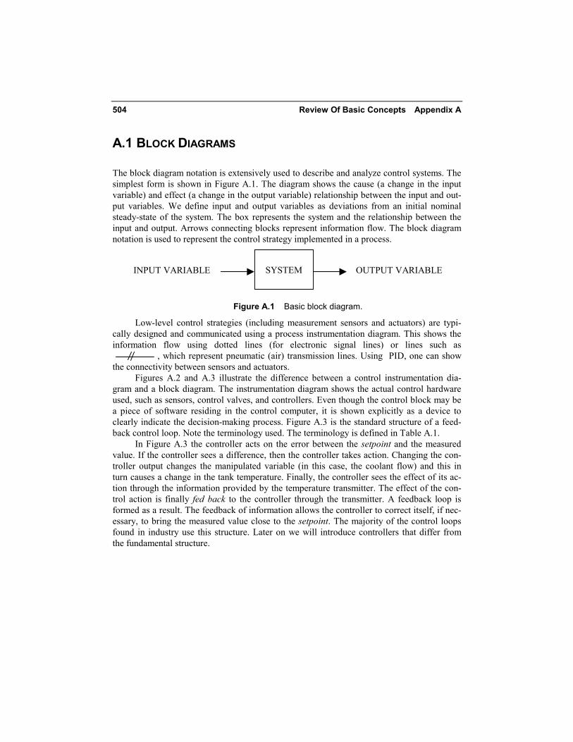
The block diagram notation is extensively used to describe and analyze control systems. The simplest form is shown in Figure A.1. The diagram shows the cause (a change in the input variable) and effect (a change in the output variable) relationship between the input and out-put variables. We define input and output variables as deviations from an initial nominal steady-state of the system. The box represents the system and the relationship between the input and output. Arrows connecting blocks represent information flow. The block diagram notation is used to represent the control strategy implemented in a process.

INPUT VARIABLE OUTPUT VARIABLE

SYSTEM

Figure A.1 Basic block diagram.

Low-level control strategies (including measurement sensors and actuators) are typi-cally designed and communicated using a process instrumentation diagram. This shows the information flow using dotted lines (for electronic signal lines) or lines such as , which represent pneumatic (air) transmission lines. Using PID, one can show the connectivity between sensors and actuators.

Figures A.2 and A.3 illustrate the difference between a control instrumentation dia-gram and a block diagram. The instrumentation diagram shows the actual control hardware used, such as sensors, control valves, and controllers. Even though the control block may be a piece of software residing in the control computer, it is shown explicitly as a device to clearly indicate the decision-making process. Figure A.3 is the standard structure of a feed-back control loop. Note the terminology used. The terminology is defined in Table A.1.

In Figure A.3 the controller acts on the error between the setpoint and the measured value. If the controller sees a difference, then the controller takes action. Changing the con-troller output changes the manipulated variable (in this case, the coolant flow) and this in turn causes a change in the tank temperature. Finally, the controller sees the effect of its ac-tion through the information provided by the temperature transmitter. The effect of the con-trol action is finally fed back to the controller through the transmitter. A feedback loop is formed as a result. The feedback of information allows the controller to correct itself, if nec-essary, to bring the measured value close to the setpoint. The majority of the control loops found in industry use this structure. Later on we will introduce controllers that differ from the fundamental structure.

A.1 Block Diagrams 505

TT101

TC101

FE101

Feed, In

Reactor Product, Out

TemperatureTransmitter Temperature

Controller

Automatic ControlValve

Manual Valve

Pneumatic Line3-15 psig

RemotelyLocated in

Control RoomElectronicTranmission Line4-20 mA current

Cooling Water, In

Figure A.2 Process instrumentation diagram of an exothermic reactor temperature control system.

CONTROL

VALVE

TANK

CONTROLLER

TRANSMITTER

Σ WATER FLOW

VALVE Tset SETPOINT

ERROR

ACTUATOR PROCESS

TEMPERATURE

Tm (MEASURED VARIABLE)

SIGNAL TO

CONTROLLER OUTPUT

MANIPULATED VARIABLE

CONTROLLED VARIABLE

+ -

Figure A.3 Block diagram of temperature control system.


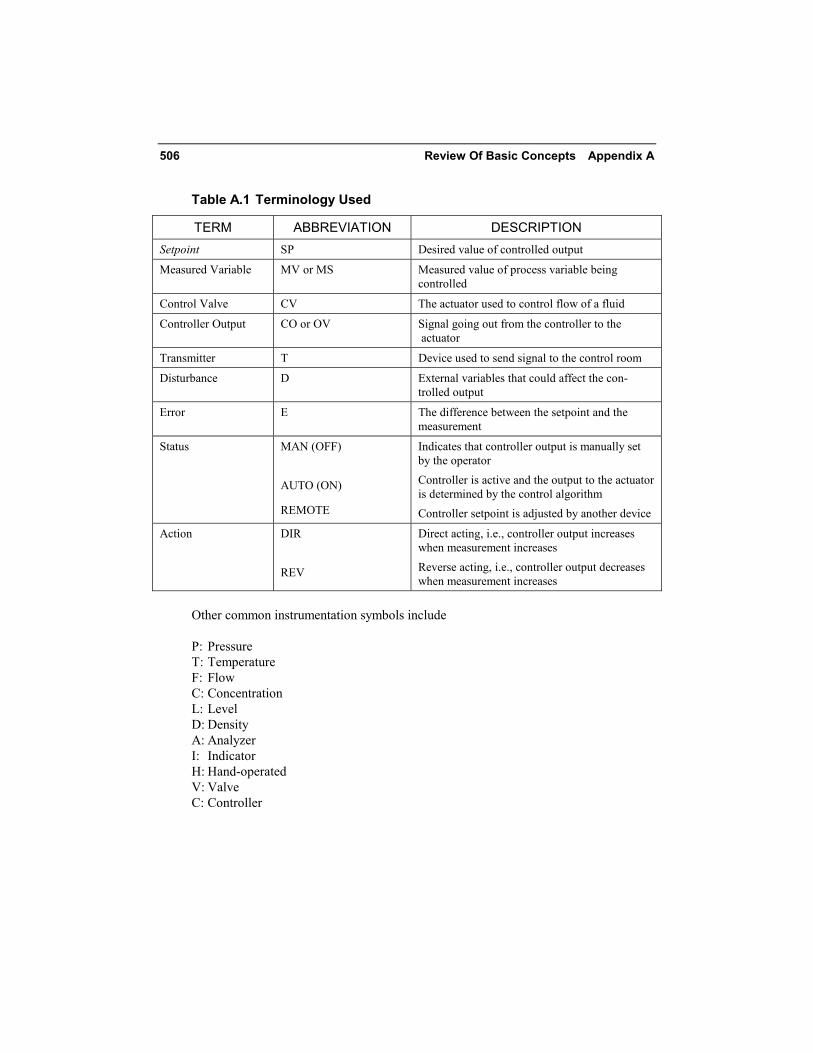
Table A.1 Terminology Used

TERM ABBREVIATION DESCRIPTION Setpoint SP Desired value of controlled output

Measured Variable MV or MS Measured value of process variable being controlled

Control Valve CV The actuator used to control flow of a fluid

Controller Output CO or OV Signal going out from the controller to the actuator

Transmitter T Device used to send signal to the control room

Disturbance D External variables that could affect the con-trolled output

Error E The difference between the setpoint and the measurement

Status MAN (OFF) AUTO (ON)

REMOTE

Indicates that controller output is manually set by the operator Controller is active and the output to the actuator is determined by the control algorithm Controller setpoint is adjusted by another device

Action DIR REV

Direct acting, i.e., controller output increases when measurement increases Reverse acting, i.e., controller output decreases when measurement increases

Other common instrumentation symbols include P: Pressure T: Temperature F: Flow C: Concentration L: Level D: Density A: Analyzer I: Indicator H: Hand-operated V: Valve C: Controller

A.2 Laplace Transform and Transfer Functions 507

A.2 LAPLACE TRANSFORM AND TRANSFER FUNCTIONS

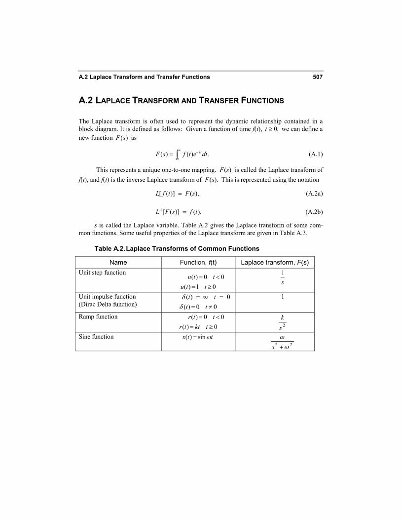
The Laplace transform is often used to represent the dynamic relationship contained in a block diagram. It is defined as follows: Given a function of time f(t), ,0≥t we can define a new function )(sF as

( ) ( ) .st

oF s f t e dt

∞ −= ∫ (A.1)

This represents a unique one-to-one mapping. )(sF is called the Laplace transform of f(t), and f(t) is the inverse Laplace transform of ).(sF This is represented using the notation

[ ( )] ( ),L f t F s= (A.2a)

1[ ( )] ( ).L F s f t− = (A.2b)

s is called the Laplace variable. Table A.2 gives the Laplace transform of some com-mon functions. Some useful properties of the Laplace transform are given in Table A.3.

Table A.2. Laplace Transforms of Common Functions

Name Function, f(t) Laplace transform, F(s) Unit step function

0 0 )( <= ttu0 1 )( ≥= ttu

s1

Unit impulse function (Dirac Delta function)

( ) 0t tδ = ∞ =0 0 )( ≠= ttδ

1

Ramp function 0 0 )( <= ttr0 )( ≥= tkttr 2s

k

Sine function ttx ω sin )( = 22 ω

ω+s


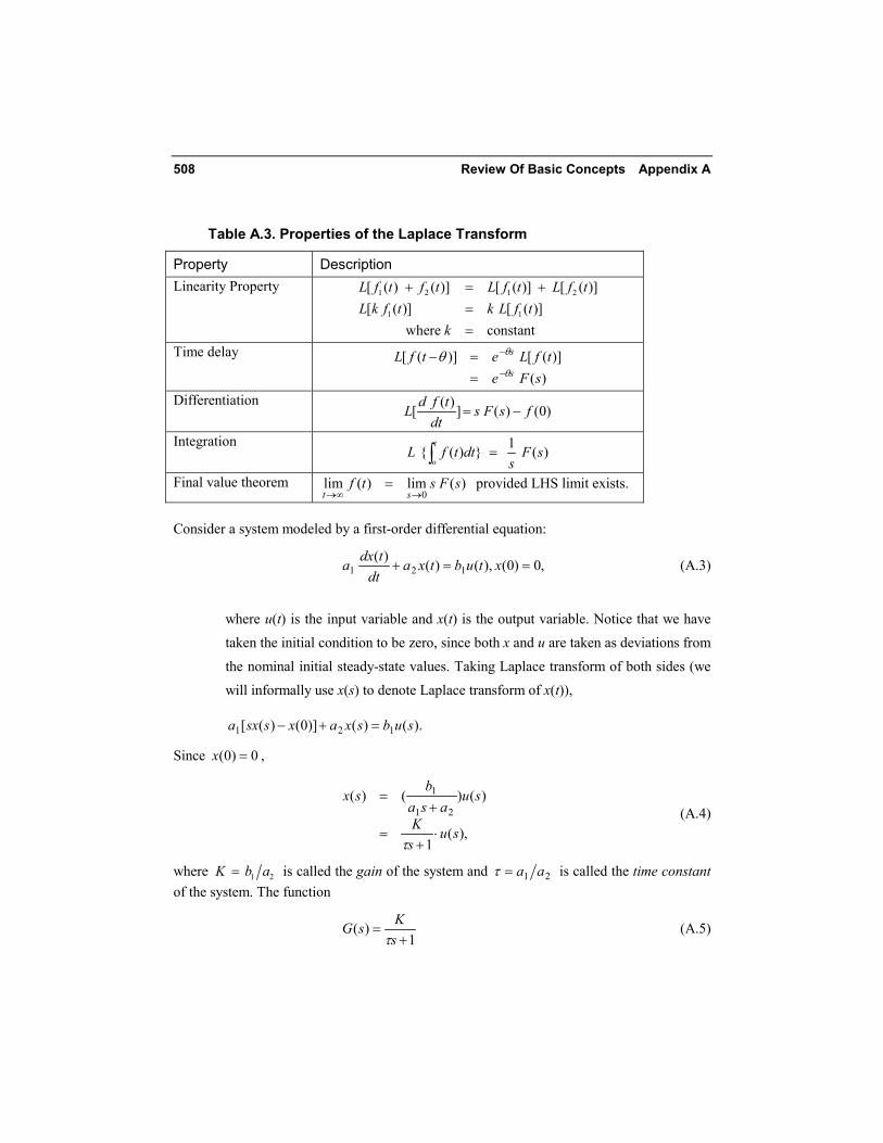
Table A.3. Properties of the Laplace Transform

Property Description Linearity Property 1 2 1 2

1 1

[ ( ) ( )] [ ( )] [ ( )][ ( )] [ ( )]

where constant

L f t f t L f t L f tL k f t k L f t

k

+ = +==

Time delay

)( )]([ )]([

sFetfLetfL

s

s

θ

θθ−

−

==−

Differentiation )0( )( ])( [ fsFs

dttfdL −=

Integration 1 { ( ) } ( )t

oL f t dt F s

s=∫

Final value theorem )( lim)( lim0

sFstfst →∞→

=

provided LHS limit exists.

Consider a system modeled by a first-order differential equation:

,0)0(),()()(121 ==+ xtubtxa

dttdxa (A.3)

where u(t) is the input variable and x(t) is the output variable. Notice that we have taken the initial condition to be zero, since both x and u are taken as deviations from the nominal initial steady-state values. Taking Laplace transform of both sides (we will informally use x(s) to denote Laplace transform of x(t)),

).()()]0()([ 121 subsxaxssxa =+− Since 0)0( =x ,

,)(

1

)()()(21

1

susK

suasa

bsx

⋅+

=

+=

τ

(A.4)

where 1 2K b a= is called the gain of the system and 21 aa=τ is called the time constant of the system. The function

1

)(+

=sKsG

τ (A.5)

A.2 Laplace Transform and Transfer Functions 509

is called the transfer function relating x(s) and u(s). The transfer function captures the dy-namic relationship between the input and output variable in a compact, convenient, and alge-braic (as opposed to the differential equation) form. )(sG is an example of a first-order transfer function, since the denominator is first-order in s. Other commonly encountered transfer functions are given below. In general, )(sG can be expressed as a ratio of polynomials:

,)()(

)(sDsNsG = (A.6a)

).()()( susGsx = (A.6b)

If the transfer function given by Eq. (A.6a) is stable, then the gain of the transfer function is defined as the steady-state change in x(t) for a unit step change in u(t), where x(t) and u(t) are the inverse Laplace transforms of x(s) and u(s). The final value theorem applied to Eq. (A.6b) shows that, by the foregoing definition, the gain of G(s) is G(0).

A.2.1 Common Transfer Functions

1. Second-Order Transfer Functions The system modeled using the differential equation

0)0(',0)0(, 2 2

22 ===++ xxKux

dtdx

dtxd τξτ (A.7a)

can be represented using the transfer function

),(1 2

)( 22 suss

sx ⋅++

=τξτ

κ (A.7b)

where time =τ constant and ξ = damping coefficient. If we can factor the denominator

),1 ( )1 ( 1 2 2122 ++=++ ssss τττξτ

where 1τ and 2τ are both real (this can be done if 1ξ > ), then we may write

).( )1

1( )1 (

)(21

suss

Ksx+

⋅+

=ττ

(A.8)

That is, the second-order system can be viewed as two first-order systems in series. Alterna-tively, we can think of the second-order differential equation being written as two equivalent, coupled, first-order differential equations.


2. Time Delay or Dead Time: se θ−

This occurs usually because of the finite time involved in fluid transportation through pipes. The output is the same as the input delayed by θ units of time. Often this is approximated using one of the Padé approximations, such as

1 2 .1 2

s ses

θ θθ

− −≈

+ (A.9

3. Lead-Lag

1

2

( 1)( ) ( )( 1)

sx s K u ss

ττ

+=

+ (A.10)

1τ is the lead time and 2τ is the lag time. 4. First Order Plus Dead Time (FOPDT)

( )( ) .1

sKe u sx ss

θ

τ

−

=+

(A.11)

This is perhaps the most frequently encountered transfer function in process control. Many process systems are approximated using this transfer function. Note the abbreviation FOPDT, used frequently in this text.

A.3 P, PI, AND PID CONTROLLER TRANSFER FUNCTIONS

In this section we will discuss the transfer functions associated with commonly used control-lers. These transfer functions have some parameters associated with them, which must be determined to yield good control system performance. The latter process of setting these controller constants is called controller tuning.

1. Proportional Control (P Control) The control law is represented by

( ) ( ) .cm t K e t m= + (A.12)

In the Laplace domain (we omit the bias term since we are dealing with deviation variables),

),()( seKsm c ⋅= (A.13)

A.3 P, PI, and PID Controller Transfer Functions 511

where m is the controller output and e(t) is the error in the control defined by

t.measuremen setpoint )( −=te (A.14)

cK is the controller gain. Note the bias term m (the steady-state controller output). This is set by the operator or initialized to the current output value when the controller is turned on. One difficulty with this controller is the choice of .m Since this is not known a priori, it is usually not possible to drive )(te to zero to eliminate steady-state offset in the controlled variable.

2. Proportional-Integral Control (PI Control) This control law is given by

]. )( 1 )([ )( ∫+= dtteteKtmI

c τ (A.15)

The integral or reset action allows the controller to eliminate steady-state offset. There is no need for a bias term, as the controller output will change as needed to drive e t( ) to zero. The controller transfer function is given by

).(]11[)( ses

KsmI

c τ+= (A.16)

Iτ is called the integral time constant and determines the weight given to the integral action relative to the proportional part.

3. Proportional-Integral-Derivative (PID) Control The ideal form of the three-mode PID controller is

]. 1 )([ )( ∫ ++=dtdedteteKtm D

Ic τ

τ (A.17)

This adds another parameter Dτ , called the derivative time constant. The transfer function of the ideal PID controller is given by

).()11()( sess

Ksm DI

c ττ

++= (A.18a)

However, because of the difficulty with differentiating noisy signals, actual industrial con-troller implementations vary from the ideal form. This is done by adding a noise filter (typi-cally a first-order lag transfer function) before derivative action is applied. A typical imple-mentation of a real PID controller would be as follows:

),()1

11()( sess

sKsm

D

D

Ic +

++=ατ

ττ

(A.18b)


where α is typically chosen as a number between .05 and 0.2, depending on the manufacturer of the controller. In some digital control systems the user has control over the value of α. Larger values of α lead to stronger filtering of the derivative action of the controller. Another form of PID controller still found in older industrial applications is the industrial form of a PID controller, so called because prior to digital control computers it was the mostcommon form of PID controller. The industrial form of a PID controller is given by

)())1(

)1()11()( *

*

* ses

ss

KsmD

D

Ic +

++=

αττ

τ (A.18c)

The controller given by Eq. (A.18c) is not as general as that given by Eq. (A.18b) since the zeros of Eq. (A.18c) are necessarily real, while those of Eq. (A.18b) may be either real or complex. In the case where the zeros of Eq. (A.18b) are real, then the relationship between the parameters of equations (A.18b) and (A.18c) are

,**DIDI ττττ = (A.18d)

.**DII τττ += (A.18e)

Solving for τD in terms of *Iτ and *

Dτ gives

)./( ****DIDID τττττ += (A.18f)

From the equation series (A.18), changing either *Iτ or *

Dτ changes both Iτ and Dτ . There-fore, the controller given by Eq. (A.18e) is often called an interacting form of the PID con-troller.

There are many other versions for the real PID controllers, but we will not discuss them here. All of the previously mentioned controllers focus on controlling a single output variable using a single manipulated input variable. Hence they are known as SISO control systems.

A.4 STABILITY OF SYSTEMS

The addition of a feedback controller to a process can alter the stability characteristics of the system. We define a system as stable if the output of the system is bounded (finite) for bounded inputs. Since stability is an important characteristic of control systems, we need some tools to analyze the stability of control systems and to evaluate the effect of controller parameters on stability.

Consider a system containing the transfer function

A.4 Stability of Systems 513

).()(

)( sxps

Ksy−

= (A.19)

If the system is forced by an impulse input given by the Dirac Delta function

,1)(),()( == sxttx δ (A.20)

then

,)(ps

Ksy−

=

which, when inverted back into the time domain, yields,

( ) .pty t Ke= (A.21)

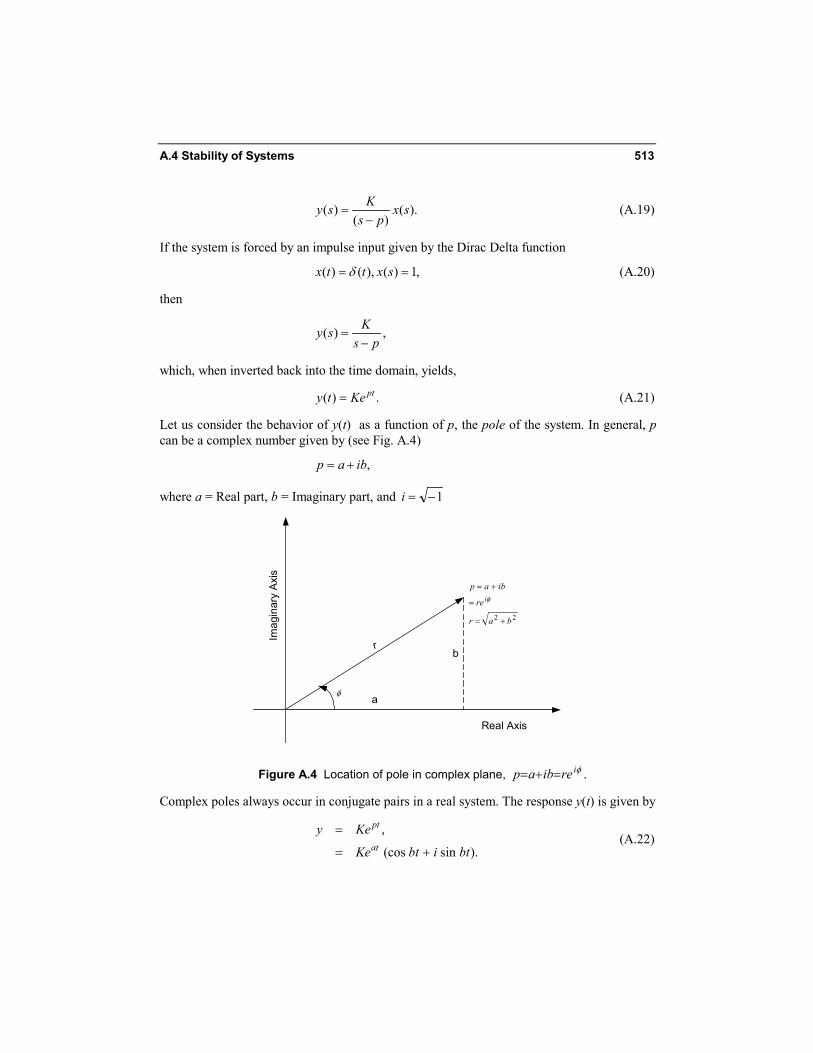
Let us consider the behavior of y(t) as a function of p, the pole of the system. In general, p can be a complex number given by (see Fig. A.4)

,ibap +=

where a = Real part, b = Imaginary part, and 1−=i

22 bar

re

ibapi

+=

=

+=φ

a

br

Real Axis

Imag

inar

y Ax

is

φ

Figure A.4 Location of pole in complex plane, .φireibap =+=

Complex poles always occur in conjugate pairs in a real system. The response y(t) is given by

,

(cos sin ).

pt

at

y Ke

Ke bt i bt

=

= + (A.22)


The imaginary part of the output will be cancelled by the conjugate pole. Let us examine the asymptotic behavior of )(ty as ∞→t .

1. If b = 0, response is not oscillatory, If b ≠ 0, response is oscillatory 2. If a > 0 ( )ty grows unbounded as ∞→t , If a < 0, ( )ty decays to zero as ∞→t

Systems whose outputs grow unbounded as ∞→t for any bounded input-forcing function are called unstable. A necessary condition for stability is that all the poles of the system have negative real parts. A typical transfer function can be expressed as a ratio of polynomials,

( )( ) ,( )

N sG sD s

= (A.23)

where N(s) = numerator polynomial in s, D(s) = denominator polynomial in s. Let

),)...()(()( 21 npspspssD −−−= (A.24)

where nppp ,...,, 21 are the roots of the polynomial D(s). These are called the poles of the system. We can expand G(s) in a partial fraction expansion as

,.......

,)),.......()((

)(

,)()(

)(

2

2

1

1

21

n

n

n

psK

psK

psK

pspspssN

sDsNsG

−++

−+

−=

−−−=

=

(A.25)

provided ,, 21 pp and np are all unique. Otherwise, the expansion must be modified slightly. If this process is perturbed by an impulse input, then

.....

),(),()()(

1

1

n

n

psK

psKsG

sxsGsy

−++

−=

=⋅=

Inverting,

....)( 11

tpn

tp neKeKty ++= (A.26)

A.4 Stability of Systems 515

Thus the behavior of )(ty is characterized by its poles. If any pole has a real part that is posi-tive, the output will grow unbounded. This leads to the following conclusion:

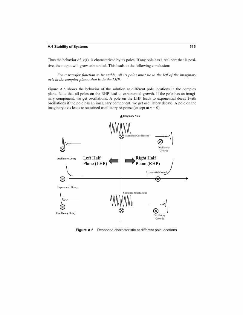
For a transfer function to be stable, all its poles must lie to the left of the imaginary axis in the complex plane; that is, in the LHP. Figure A.5 shows the behavior of the solution at different pole locations in the complex plane. Note that all poles on the RHP lead to exponential growth. If the pole has an imagi-nary component, we get oscillations. A pole on the LHP leads to exponential decay (with oscillations if the pole has an imaginary component, we get oscillatory decay). A pole on the imaginary axis leads to sustained oscillatory response (except at s = 0).

⊗

⊗

⊗

⊗

⊗ ⊗

⊗

⊗

Imaginary Axis

OscillatoryGrowth

Exponential Growth

OscillatoryGrowth

Exponential Decay

Oscillatory Decay

Oscillatory Decay

Sustained Oscillations

Right HalfPlane (RHP)

Left HalfPlane (LHP)

⊗

⊗

⊗

⊗

⊗

⊗

Imaginary Axis

Oscillatory Decay

Oscillatory Decay

Right HalfPlane (RHP)

Left HalfPlane (LHP)

Sustained Oscillations

Figure A.5 Response characteristic at different pole locations


A.5 STABILITY OF CLOSED-LOOP SYSTEMS

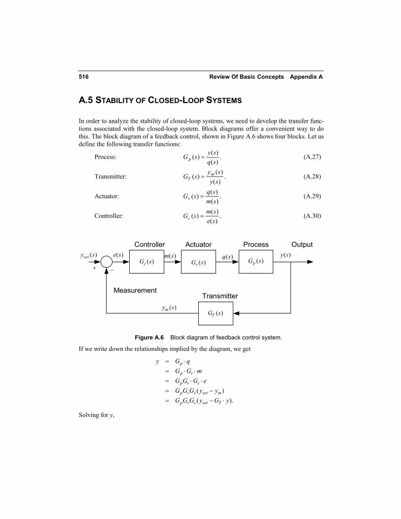
In order to analyze the stability of closed-loop systems, we need to develop the transfer func-tions associated with the closed-loop system. Block diagrams offer a convenient way to do this. The block diagram of a feedback control, shown in Figure A.6 shows four blocks. Let us define the following transfer functions:

Process: .)()(

)(sqsysG p = (A.27)

Transmitter: .)()(

)(sysy

sG mT = (A.28)

Actuator: .)()(

)(smsqsGv = (A.29)

Controller: .)()(

)(sesmsGc = (A.30)

( )cG s ( )vG s ( )pG s

( )TG s

+ −

( )e s ( )m s ( )q s ( )y s

( )my s

Controller

MeasurementTransmitter

ProcessActuator( )sety s

Output

Figure A.6 Block diagram of feedback control system.

If we write down the relationships implied by the diagram, we get

).()(

yGyGGGyyGGG

eGGGmGG

qGy

Tsetcvp

msetcvp

cvp

vp

p

⋅−=−=

⋅⋅=⋅⋅=

⋅=

Solving for y,

A.5 Stability of Closed-Loop Systems 517

,1

p v cset

p v c T

G G Gy y

G G G G=

+ (A.31)

,)( setCL ysG ⋅= (A.32)

where )(sGCL is called the closed-loop transfer function. Note the following: 1. The stability of the closed-loop is determined by the roots of the polynomial

.01 =+ Tvcp GGGG (A.33)

This is called the characteristic equation of the closed-loop system. 2. The controller transfer function will alter the poles of the closed-loop system. The

roots of this equation (also referred to as zeros of the polynomial) are the poles of the closed-loop system.

3. A rule that is useful to remember is that for negative feedback, the closed-loop transfer function can be written as

loop in the functions transfer ofproduct 1output theosetpoint t thefrompath forwardon the blocksin functions transfer ofproduct

+

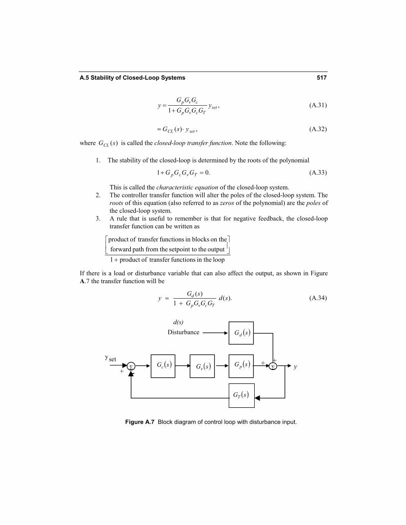
If there is a load or disturbance variable that can also affect the output, as shown in Figure A.7 the transfer function will be

( ) ( ).

1 d

p v c T

G sy d sG G G G

=+

(A.34)

Disturbance

+ + y Σ Σ + -

y set

d(s)

( )sGc ( )sGv( )sGp

( )sGT

( )sGd

Figure A.7 Block diagram of control loop with disturbance input.


Example A.1 First-Order with PI Control

Let

.1)()(

),11()(

,)1(

)(

==

+=

+=

sGsGs

KsG

sK

sG

Tv

Icc

pp

τ

τ

This leads to the closed loop transfer function

,)1((

)1()(

12

1

1

pcpc

pc

setCL

KKsKKs

sKKy

ysG+++

+==

τττ

τ (A.35)

with a steady-state gain .1)0( =CLG Hence no steady-state error (offset) will be present for a step change in the setpoint.

♦

Example A.2 Third-Order Process with P Control

For a process with transfer functions

)3)(2)(1(

1)(+++

=sss

sG p , ,1)()(,)( === sGsGKsG Tvcc (A.36)

the closed-loop response is given by the equation

.)3)(2)(1( c

c

set KsssK

yy

++++= (A.37)

The characteristic equation is given by

.0)3)(2)(1( =++++ cKsss (A.38)

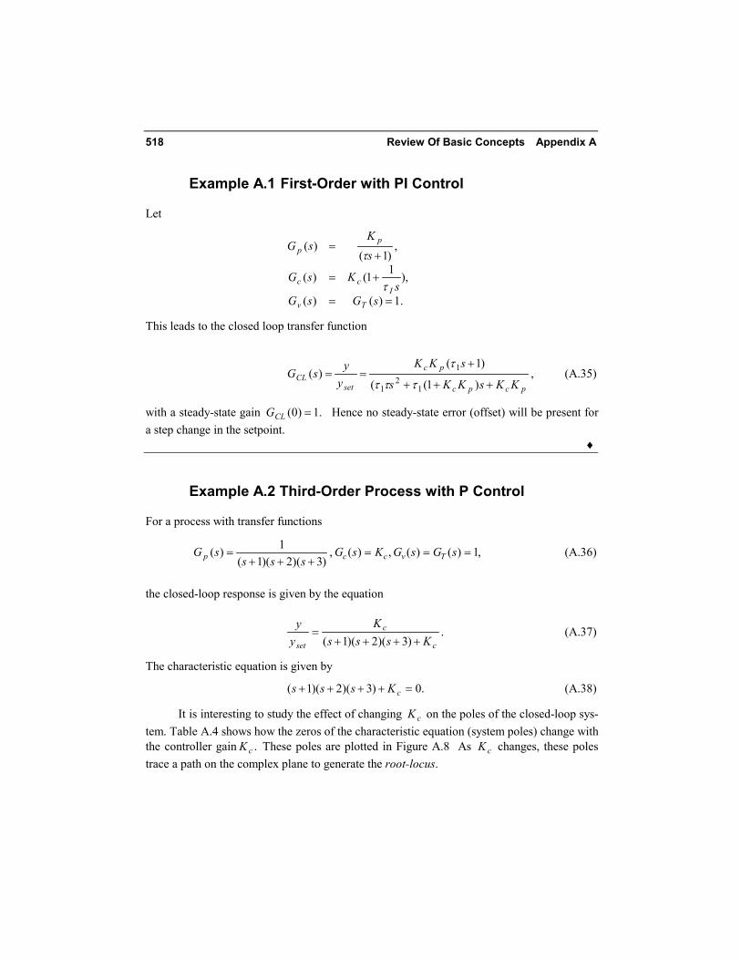
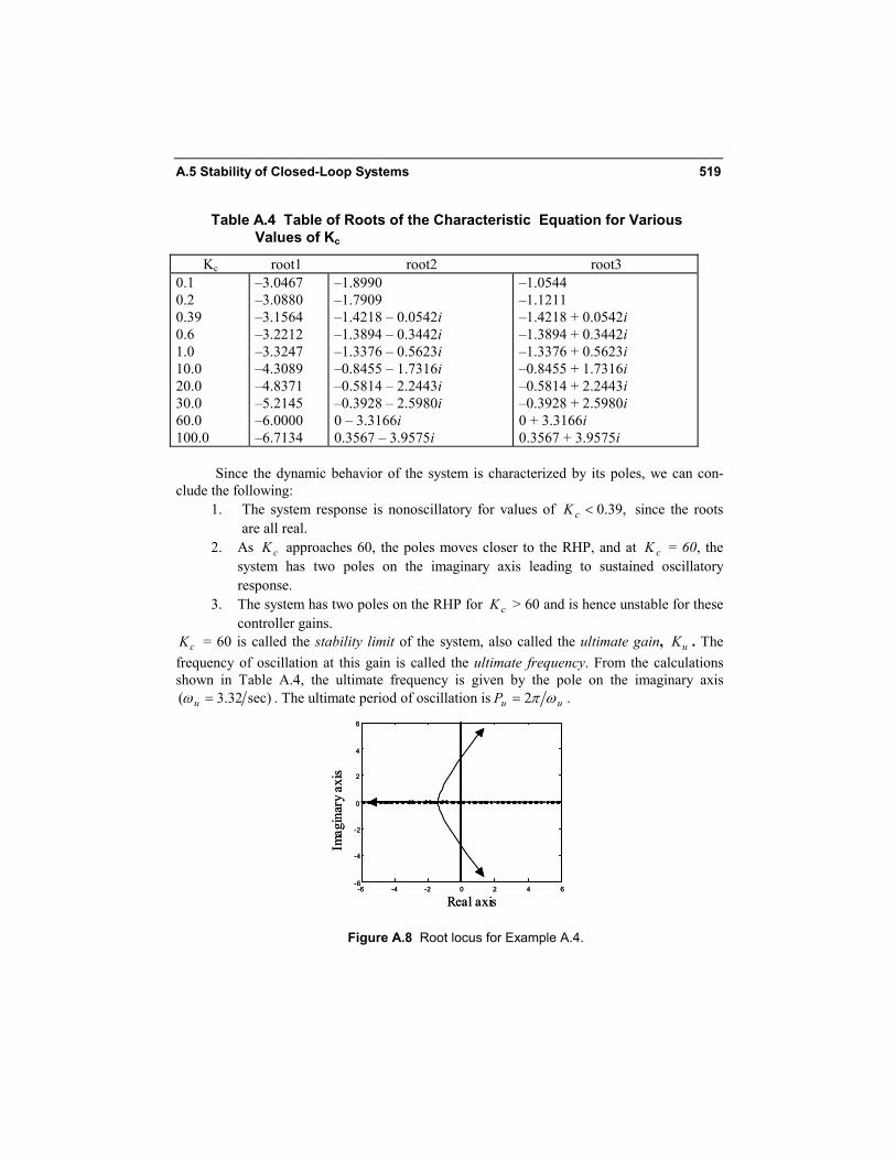
It is interesting to study the effect of changing cK on the poles of the closed-loop sys-tem. Table A.4 shows how the zeros of the characteristic equation (system poles) change with the controller gain .cK These poles are plotted in Figure A.8 As cK changes, these poles trace a path on the complex plane to generate the root-locus.

A.5 Stability of Closed-Loop Systems 519

Table A.4 Table of Roots of the Characteristic Equation for Various Values of Kc

Kc root1 root2 root3 0.1 0.2 0.39 0.6 1.0 10.0 20.0 30.0 60.0 100.0

–3.0467 –3.0880 –3.1564 –3.2212 –3.3247 –4.3089 –4.8371 –5.2145 –6.0000 –6.7134

–1.8990 –1.7909 –1.4218 – 0.0542i –1.3894 – 0.3442i –1.3376 – 0.5623i –0.8455 – 1.7316i –0.5814 – 2.2443i –0.3928 – 2.5980i 0 – 3.3166i 0.3567 – 3.9575i

–1.0544 –1.1211 –1.4218 + 0.0542i –1.3894 + 0.3442i –1.3376 + 0.5623i –0.8455 + 1.7316i –0.5814 + 2.2443i –0.3928 + 2.5980i 0 + 3.3166i 0.3567 + 3.9575i

Since the dynamic behavior of the system is characterized by its poles, we can con-clude the following:

1. The system response is nonoscillatory for values of ,39.0<cK since the roots are all real.

2. As cK approaches 60, the poles moves closer to the RHP, and at cK = 60, the system has two poles on the imaginary axis leading to sustained oscillatory response.

3. The system has two poles on the RHP for cK > 60 and is hence unstable for these controller gains.

cK = 60 is called the stability limit of the system, also called the ultimate gain, uK . The frequency of oscillation at this gain is called the ultimate frequency. From the calculations shown in Table A.4, the ultimate frequency is given by the pole on the imaginary axis

)sec32.3( =uω . The ultimate period of oscillation is .2 uuP ωπ=

-6 -4 -2 0 2 4 6-6

-4

-2

0

2

4

6

Real axis

Imag

inar

y ax

is

-6 -4 -2 0 2 4 6-6

-4

-2

0

2

4

6

Real axis

Imag

inar

y ax

is

Figure A.8 Root locus for Example A.4.


A.6 CONTROLLER TUNING

PID controllers are used in the majority of SISO feedback controllers because of their effec-tiveness and simplicity. The transfer function of a typical PID controller is given by

).())1(

111()( sesss

Ksm DI

c τατ +

++= (A.39)

Controller tuning refers to determining the appropriate values of , , andc I DK τ τ α in the controller transfer function. While there is no single “right” way to choose PID parameters, the reader should be aware that the literature is full of wrong ways. Until relatively recently, all controller tuning algorithms were based on the local behavior of the process at the time of tuning. However, local behavior of a process usually changes as operating conditions change due to disturbances, setpoint changes, and process aging. Since most real processes are nonlinear in their global behavior, their local behavior changes as the operating point changes. Thus, a well-tuned controller at one operating point might behave very badly at an-other. The concept of process uncertainty is one way of attempting to mathematically de-scribe the variations of local process behavior over an operating region in a way that is useful for controller tuning. While it is usually not easy to obtain accurate uncertainty descriptions, it is often possible to obtain reasonable estimates that allow much better tuning than would otherwise be possible. Chapters 7 and 8 present relatively simple methods for including proc-ess uncertainty in the tuning of one-degree and two-degree of freedom IMC controllers. The tuned IMC controllers can then be converted into PI or PID controllers, using the techniques of Chapter 6.

In the next section we review the traditional controller tuning methods that are based on local process behavior. Our reasons for doing so are that these methods are still used, even though better methods are available (see chapters 6, 7, and 8), and it is important for the reader to be familiar with these methods in order to be able to communicate with plant engi-neers and possibly convince them to convert to better methods.

A.6.1 Tuning Correlations

A number of authors have published empirical correlations for tuning PID controllers based on the selected performance criteria and assumed process model structure. The FOPDT model is used most often. Generally, correlations are provided in terms of the process gain, the time constant, and time delay in the FOPDT model. Separate correlations are provided for servo control and regulatory control. Different criteria are used to evaluate the perform-ance, including

1. Integral Squared Error (ISE)

∫∞

=0

2dteISE (A.40)

A.6 Controller Tuning 521

This criterion is widely used in optimal control theory. It is also the criterion of choice in many industrial implementations of model-predictive control (MPC).

2. Integral Absolute Error (IAE)

o

IAE e dt∞

= ∫ (A.41)

3. Integral Time Average Error (ITAE)

o

ITAE e tdt∞

= ∫ (A.42)

A few of the well-known correlations follow.

1. Reaction Curve Method (Ziegler-Nichols, 1942)

For a system modeled using an FOPDT transfer function,

1 )(

+=

−

sKesG

s

τ

θ

(A.43)

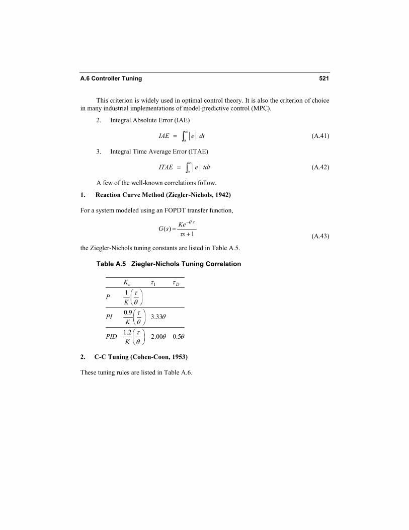
the Ziegler-Nichols tuning constants are listed in Table A.5.

Table A.5 Ziegler-Nichols Tuning Correlation

1

1

0.9 3.33

1.2 2.00 0.5

c DK

PK

PIK

PIDK

τ ττθτ θθτ θ θθ

2. C-C Tuning (Cohen-Coon, 1953) These tuning rules are listed in Table A.6.


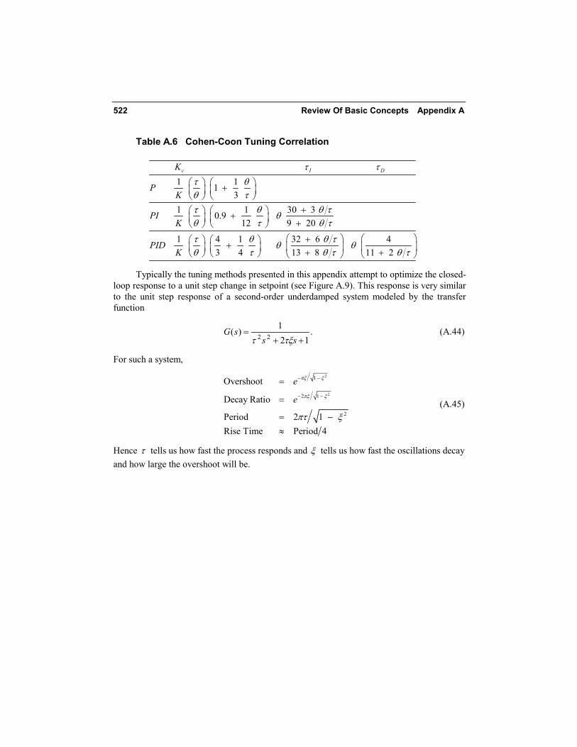
Table A.6 Cohen-Coon Tuning Correlation

1 1 1 3

1 1 30 3 0.9 12 9 20

1 4 1 32 6 4 3 4 13 8 11 2

c I DK

PK

PIK

PIDK

τ ττ θθ ττ θ θ τθθ τ θ τ

τ θ θ τθ θ

θ τ θ τ θ τ

+

+ + +

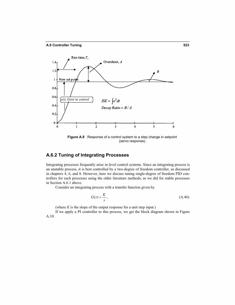
+ + + + Typically the tuning methods presented in this appendix attempt to optimize the closed-

loop response to a unit step change in setpoint (see Figure A.9). This response is very similar to the unit step response of a second-order underdamped system modeled by the transfer function

.12

1)(22 ++

=ss

sGτξτ

(A.44)

For such a system,

2

2

1

2 1

2

Overshoot

Decay Ratio

Period 2 1Rise Time Period 4

e

e

πξ ξ

πξ ξ

πτ ξ

− −

− −

=

=

= −≈

(A.45)

Hence τ tells us how fast the process responds and ξ tells us how fast the oscillations decay and how large the overshoot will be.

A.6 Controller Tuning 523

0

0.2

0.4

0.6

0.8

1

1.2

1.4

0 1 2 3 4 5 6

New set point

Overshoot, ARise time, Tr

B

e(t), Error in control 2

/

ISE e dt

Decay Ratio B A

=

=∫

0

0.2

0.4

0.6

0.8

1

1.2

1.4

0 1 2 3 4 5 6

New set point

Overshoot, ARise time, Tr

B

e(t), Error in control 2

/

ISE e dt

Decay Ratio B A

=

=∫

Figure A.9 Response of a control system to a step change in setpoint (servo response).

A.6.2 Tuning of Integrating Processes

Integrating processes frequently arise in level control systems. Since an integrating process is an unstable process, it is best controlled by a two-degree of freedom controller, as discussed in chapters 4, 6, and 8. However, here we discuss tuning single-degree of freedom PID con-trollers for such processes using the older literature methods, as we did for stable processes in Section A.6.1 above.

Consider an integrating process with a transfer function given by

,)(sKsG = (A.46)

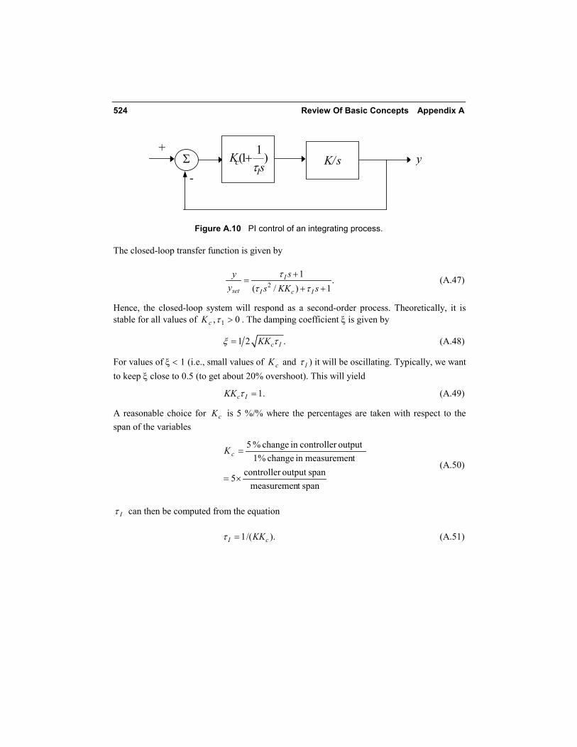
(where K is the slope of the output response for a unit step input.) If we apply a PI controller to this process, we get the block diagram shown in Figure

A.10.


y Σ

+

- s/K

1(1 )cI

Ksτ

+

Figure A.10 PI control of an integrating process.

The closed-loop transfer function is given by

21

.( / ) 1

I

set I c I

syy s KK s

ττ τ

+=

+ + (A.47)

Hence, the closed-loop system will respond as a second-order process. Theoretically, it is stable for all values of 0, 1 >τcK . The damping coefficient ξ is given by

1 2 .c IKKξ τ= (A.48)

For values of ξ < 1 (i.e., small values of cK and 1τ ) it will be oscillating. Typically, we want to keep ξ close to 0.5 (to get about 20% overshoot). This will yield

1.c IKK τ = (A.49)

A reasonable choice for cK is 5 %/% where the percentages are taken with respect to the span of the variables

spant measuremenspanoutput controller5

t measuremenin change 1%output controllerin change % 5

×=

=cK (A.50)

Iτ can then be computed from the equation

1/( ).I cKKτ = (A.51)

A.7 Regulatory Issues Introduced by Constraints 525

A.7 REGULATORY ISSUES INTRODUCED BY CONSTRAINTS

In this section we examine regulatory issues that can be derived from the process model. The focus is on steady-state suppression of disturbances for SISO systems. We examine the dy-namic suppression issues in Appendix B. For convenience in the analysis we consider first the representation of models using dimensionless variables.

A.7.1 Scaling and Nondimensionalization of Process Vari-ables

Control engineers have long practiced the scaling of variables using the span of the instru-ment used to measure that variable (the maximum and minimum measurable values of that variable). For a measurement y, the scaling is defined as

,minmax yy

yyy measmeas

−−

= (A.52)

where minmax yy − is the span of the measuring instrument (a field adjustable quantity). The smaller the span, the greater the accuracy of the instrument. During startup and shutdown phases, a greater range of the measurement is expected and the span may be kept large.

measy is the normal steady-state value of the variable. Ideally, this should be set to the mid-dle of the span to yield a range of

.5.05.0 ≤≤− y A similar definition is used to scale manipulated input variables. With control valves,

the nominal steady-state valve is kept closer to 1 (say in the 65% to 75% open range) to re-duce pressure losses.

A.7.2 Steady-State Suppression of Disturbances for SISO Systems

Consider SISO system, as shown in Figure A.11. The transfer function model is

)()()()( sdsuspsy += . (A.53)

The control objective is to maintain y close to its nominal steady-state value of 0 in presence of disturbances. First we consider the steady-state case. The problem reduces to

).()()()( odouopsy += (A.54)


( )p s

( )d s

( )u s( )y s

Figure A.11 Process with disturbance

The ability to regulate the process can be determined by the graph shown in Figure A.12.

u

y

maxuminu

miny

maxySlope = p(0)

ControllableRange of y

Figure A.12 The effect of input constraints on output.

The figure shows that for a low gain system in which (p(0) is small the “reachable space” of y is limited or small in size. If the effect of the disturbance exceeds this limit, then y cannot be regulated; that is, we cannot reach the desired setpoint in the steady-state. A large value of p(0) implies that the process is very sensitive to small changes in the input u. Usually, there is an uncertainty or error associated with implementing a control action. In this case the process will amplify that uncertainty and this could lead to difficulty in regulation. Ideally, therefore, a gain closer to 1 will usually be a compromise between sensitivity to input uncer-tainty and ability to regulate in presence of disturbances.

A.7 Regulatory Issues Introduced by Constraints 527

Example A.3 Steady-State Disturbance Suppression in a Distillation Column

Consider the column for separating a mixture of methanol/water. The nominal steady-state operating conditions are shown. Given the following steady-state observations, determine the steady-state regulation of the bottom product purity using the reboiler heat duty and the dis-tillate flow rate when the feed can vary from 95 to 105 lb moles/hr.

Condition Feed Rate

F

Distillation Rate D

Reboiler Duty

MM Btu/hrQ

Top Purity XT

Mole Frac-tion

Bottom Pu-rity XB

Mole Frac-tion

Span or Range of Variable

0-200 lb moles/hr

0 -100 lb mole/hr

0-4 MMBtu/hr

0-0.02 0-0.2

Nominal Steady-state

100 45 2.2 .0057 .0955

Perturb D 100 46 2.2 .0063 .0794 Perturb Q 100 45 2.3 .0047 .0948 Perturb F 105 45 2.2 .0058 .1292

Solution

We compute the steady-state gains of the process in non-dimensional, scaled variables:

111 12

21 22 2

,fT

B f

kx k k df

x k k q k

= +

.200,100)(

,4)(,2.0)(,)02.0()(

FfDDdQQqXXxXXx BBBTTT

=−=

−=−=−=

From the data given

12 11 21 22

(.0047 .0057) (0.02) 2, 3.0, 8.05, .14,(2.3 2.2) 4.0

k k k k−= = − = = = −

−

yielding

.74.64.0

,14.05.820.3

=

−−

= fkK


The variations in Bx caused by the feed flow disturbance can be computed as 6.74*5 / 200 0.1685.± = ± Using q, the maximum variations achievable in Bx is given by (0.14)*50 /100 .07.± = ± Hence we conclude that it is not possible to regulate xB using q

because of the small gain.

However, the variations in Bx that can be achieved using d are 8.05*(4 23) / 4 3.4.± − = ± Hence xB can be regulated easily, using d. Note that this result is

counterintuitive, since our first instinct would be to choose to regulate xB using q (due to the physical proximity of the two variables).

♦

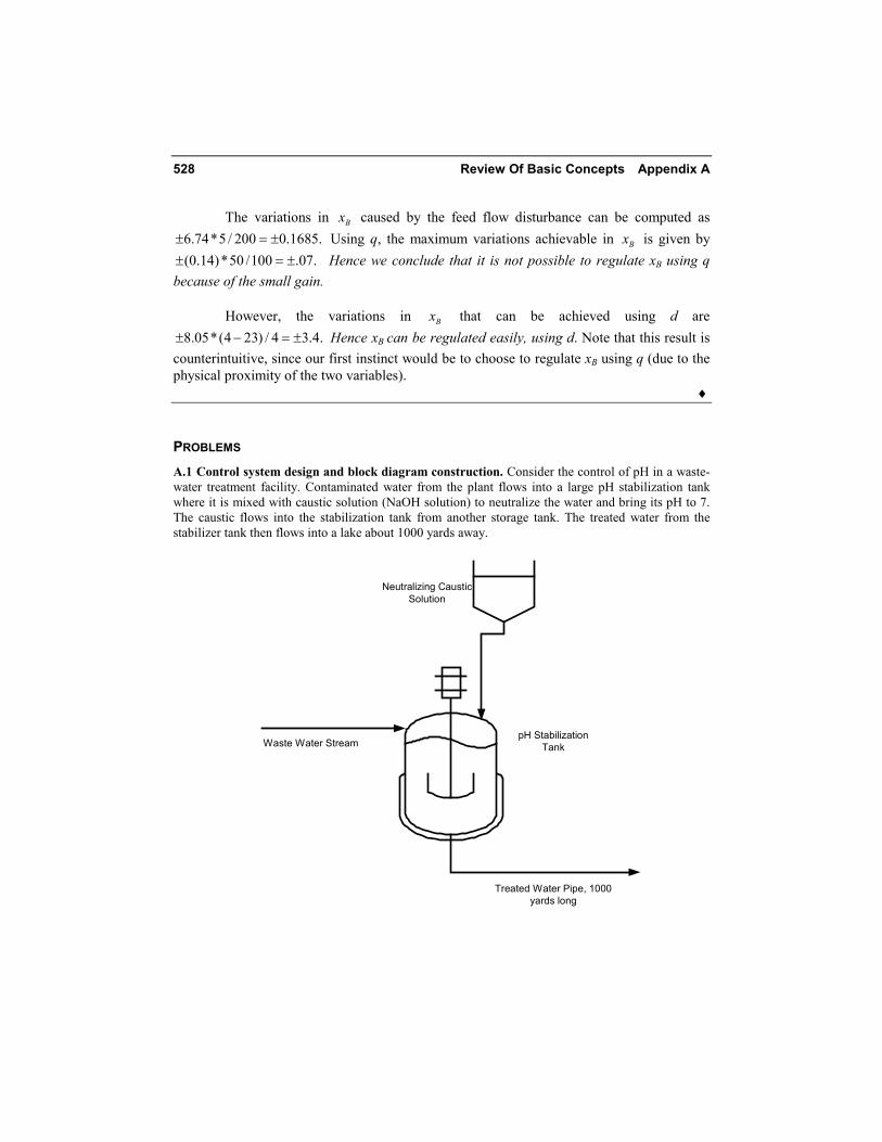
PROBLEMS A.1 Control system design and block diagram construction. Consider the control of pH in a waste-water treatment facility. Contaminated water from the plant flows into a large pH stabilization tank where it is mixed with caustic solution (NaOH solution) to neutralize the water and bring its pH to 7. The caustic flows into the stabilization tank from another storage tank. The treated water from the stabilizer tank then flows into a lake about 1000 yards away.

Waste Water Stream

Treated Water Pipe, 1000yards long

pH StabilizationTank

Neutralizing CausticSolution

Problems 529

a. Design a feedback control system to control the pH of the water being discharged to the lake. Show the process instrumentation diagram using standard symbols. Identify and label all sensors, transmitters and control valves.

b. Draw a block diagram of the pH control system, identifying all variables used.

c. Discuss briefly the pros and cons of the following options from the point of view of the per-formance of the control system. (i) Place the pH sensor in the pipe through which treated water is leaving the stabilization tank. Sensor is located as close to the tank as possible.(ii) Place the pH sensor at the point where the wastewater enters the lake. (iii) Place the pH sen-sor inside the stabilization tank. (iv) Place the pH sensor in the pipe that brings the water into the stabilization tank.

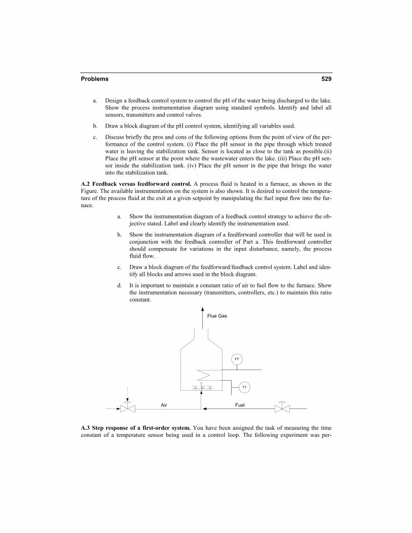
A.2 Feedback versus feedforward control. A process fluid is heated in a furnace, as shown in the Figure. The available instrumentation on the system is also shown. It is desired to control the tempera-ture of the process fluid at the exit at a given setpoint by manipulating the fuel input flow into the fur-nace.

a. Show the instrumentation diagram of a feedback control strategy to achieve the ob-jective stated. Label and clearly identify the instrumentation used.

b. Show the instrumentation diagram of a feedforward controller that will be used in conjunction with the feedback controller of Part a. This feedforward controller should compensate for variations in the input disturbance, namely, the process fluid flow.

c. Draw a block diagram of the feedforward/feedback control system. Label and iden-tify all blocks and arrows used in the block diagram.

d. It is important to maintain a constant ratio of air to fuel flow to the furnace. Show the instrumentation necessary (transmitters, controllers, etc.) to maintain this ratio constant.

Flue Gas

Air Fuel

TT

FT

A.3 Step response of a first-order system. You have been assigned the task of measuring the time constant of a temperature sensor being used in a control loop. The following experiment was per-


formed. The sensor was initially at room temperature of 25 °C. It was suddenly inserted into hot water in a cup. You read the temperature as 40 °C after 1 minute. The reading reached a steady-state value of 45 C after a few minutes. Assume the sensor can be modeled as a first-order system.

a. Estimate the time constant of the temperature sensor.

b. Write the transfer function for the temperature sensor. Use your result from Part a. Show that the gain is 1.

c. If the temperature can be read accurately to ± 1 °C on the sensor, what is the accuracy of your time constant estimate in minutes?

A.4 Step response of a first-order system. A bare thermocouple, when suddenly moved from a steady temperature of 80°F into a stream of hot air at a constant temperature of 100°F, reads 90°F after 1 sec. Assume the thermocouple responds as a first-order system.

a. Sketch the behavior of the temperature surrounding the thermocouple as a function of time.

b. Sketch the expected behavior of the measured temperature as a function of time (qualita-tively).

c. What will be the final (steady-state) temperature measured by the thermocouple?

d. Compute the measured temperature at 2 sec.

A.5 Pulse response of a first-order system. The time-dependent behavior of the outlet concentration of a stirred tank to changes in inlet concentration is given by

,xydtdy

=+τ

where y = outlet tank concentration, x = inlet concentration t = time in minutes.

Suppose at t = 0, y = 0. The inlet concentration is suddenly increased from 0 to 1 and maintained at 1 for the duration of 1 minute, at which time it is brought back to zero. This is called a unit pulse input.

a. Sketch x(t) as a function of time.

b. Write an equation for x(t) in terms of unit step functions.

c. What is the Laplace transform of x(t)?

d. What is the Laplace transform of y(t)?

e. Solve for y(t) by inverting the result of Part d.

f. If τ = 1, sketch the response y(t).

A.6 Inverting Laplace transforms. Sketch the behavior of f(t) if its Laplace transform is given by

2 3

21( ) .

s s se e eF ss ss

− − −−= + −

A.7 Using dynamic response characteristics in design. A holding tank of uniform cross section has been designed to smooth out the flow from a reactor to a purification column. The reactor has to be shut down periodically for cleaning. Given the following data, estimate the maximum rate of change of

Problems 531

the flow into the column. Assume flow out of the holding tank is proportional to the height of liquid in the holding tank.

Data: The tank has a cross-sectional area of 10 ft2 and a height of 10 ft. Normal (steady-state level) in the tank is 5 ft. The normal flow from the reactor is 5 ft3/hr and the reactor is periodically shut down for 2 hours.

Hint: First write the model of the holding tank. Then derive a transfer function relating changes in inlet flow to the outlet flow. It is preferable to use deviation variables. This is a first-order transfer function. Shutting down the reactor reduces the inlet flow to 0 suddenly. Hence it is a step change. The outlet flow responds to this step change. Sketch its response. When is the slope of this curve a maximum?

A.8 Closed-loop stability. An open-loop unstable process can be represented by the following trans-fer function:

( ) .(4 1)( 1)( 1)v T

KG ss s sτ τ

=− + +

where vτ and Tτ are, respectively, the time constants of the control valve and the transmitter. Assum-

ing proportional control with gain cK is used, find the range of the loop gain cKK for which the loop is stable if

a. The valve and transmitter time constants are negligible ( 0).v Tτ τ= =

b. The valve time constant is negligible, and .min0.1=Tτ

A.9 Response of second-order systems. The temperature of a reactor responds to the feed variations as a second-order system. Let

)(tT = deviation of reactor temperature from steady-state,

)(tF = deviation of reactor feed flow from steady-state,

.224)15(

)()(2 ++

=ssgpmF

sFsT

The reactor is operating normally at a feed rate of 70 gpm and at 300°F. Previous experience shows that if the reactor temperature exceeds 350°F, the catalyst will be deactivated. The feed is subject to sudden step changes. What is the maximum permissible step change in the feed rate, that will keep the reactor temperature below its specified maximum of 350°F?

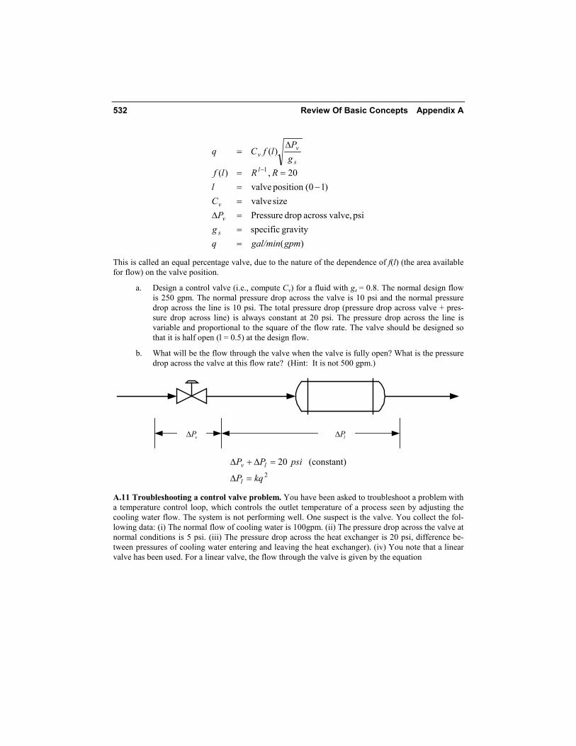
A.10 Control valve design. Control valves play an important role in the performance of the control system. This problem considers a typical case where a control valve is installed in line with a process unit, in this case a heat exchanger. The working design equation for the control valve is


)(gravity specific

psi valve,across drop Pressure size valve

)10(position valve20,)(

)(

1

gpmgal/minqg

PCl

RRlfgP

lfCq

s

v

v

ls

vv

===∆=

−===

∆=

−

This is called an equal percentage valve, due to the nature of the dependence of f(l) (the area available for flow) on the valve position.

a. Design a control valve (i.e., compute Cv) for a fluid with gs = 0.8. The normal design flow is 250 gpm. The normal pressure drop across the valve is 10 psi and the normal pressure drop across the line is 10 psi. The total pressure drop (pressure drop across valve + pres-sure drop across line) is always constant at 20 psi. The pressure drop across the line is variable and proportional to the square of the flow rate. The valve should be designed so that it is half open (l = 0.5) at the design flow.

b. What will be the flow through the valve when the valve is fully open? What is the pressure drop across the valve at this flow rate? (Hint: It is not 500 gpm.)

lP∆vP∆

2

(constant) 20

kqP

psiPP

l

lv

=∆

=∆+∆

A.11 Troubleshooting a control valve problem. You have been asked to troubleshoot a problem with a temperature control loop, which controls the outlet temperature of a process seen by adjusting the cooling water flow. The system is not performing well. One suspect is the valve. You collect the fol-lowing data: (i) The normal flow of cooling water is 100gpm. (ii) The pressure drop across the valve at normal conditions is 5 psi. (iii) The pressure drop across the heat exchanger is 20 psi, difference be-tween pressures of cooling water entering and leaving the heat exchanger). (iv) You note that a linear valve has been used. For a linear valve, the flow through the valve is given by the equation

Problems 533

( ) ,

( ) ,valve position (0-1).

vv

s

Pq C f lg

f l ll

∆=

==

The valve size C according to the specs, is 100. Valve is air-to-open (as the signal to the valve in-creases, the valve opens more).

a. What is the maximum achievable flow through the cooling water valve? Assume that the pressure drop across the heat exchanger is proportional to the square of the flow rate. The total pressure drop (the sum of the pressure drops across the valve and the heat exchanger) is a constant. (See figure in Problem A.10.)

b. Based on your calculations, could the valve be the cause of the problem with the control loop? Explain why or why not. If the valve were the cause of the problem, what remedial action would you recommend?

References

Cohen G. H., and G. A. Coon. 1953. “Theoretical Considerations of Retarded Control.” Trans. ASME, 75, 827.

Luyben, W. L. 1990. Process Modeling, Simulation and Control for Chemical Engineers. 2nd Ed. McGraw-Hill, NY.

Marlin T. E. 1995. Process Control: Designing Processes and Control Systems for Dynamic Per-formance. McGraw-Hill, NY.

Ogunnaike, B. A., and W. H. Ray. 1994. Process Dynamics, Modeling and Control. Oxford University Press, NY.

Seborg, D. E., T. F. Edgar, and D.A. Mellichamp. 1989. Process Dynamics and Control. John Wiley & Sons, NY.

Smith, C. A., and A. B. Corripio. 1985. Principles and Practice of Automatic Process Control. John Wiley & Sons, NY.

Stephanopoulos, G. 1984. Chemical Process Control. Prentice Hall, NJ.

Ziegler J. G., and N. B. Nichols. 1942. “Optimum Settings for Automatic Controllers” Trans. ASME, 64, 759.

review of basic concepts - bgu courses/appa...503 a ppendix a review of basic concepts objectives...

Documents