rt1 mountain view, ca 94043-1115 june 23, 2000 … · mountain view, ca 94043-1115 . june 23 ......
TRANSCRIPT

2685 Marine Way Suite 1314 ~ Mountain View CA 94043-1115 June 23 2000 rt1 AQUA TERRA lII (650) 962middot1864 bull Fax (650) 962middot0706
I() CONSULTANTS C5I wwwaquaterracom
Ms Susan C Svirsky US EPA New England - Region I I Congress Street Suite 1100 Boston MA 02114-2023
SUBJECT EPA Contract No 68-C-98-0 I 0 W A 2-12 A TC Project No 9820-212 Final Report on STA from GeoSea
Dear Susan
Enclosed is the Final Report from GeoSea entitled A Sediment Trend Analysis (STA) of Housatonic River Grain-Size Data for work performed under their subcontract with AQUA TERRA for this Work Assignment As requested I have provided a copy to Chris Wallen (ZZ Consulting) and Paul Craig (Dynamic Solutions) for their review and an additional unbound copy to the contract PO Tangela Cooper as required by our contract
We should plan to discuss the results and implications of this report at our meeting in Pittsfield in August Please call if you need anything else at this time or if you have any questions or comments
Very truly yours AQUA TERRA Consultants
Anthony S Donigian Jr PE President amp Principal Engineer
Enclosure Filec198201W A212IGeoSeaFinaIReportlel wpd cc T Cooper - EPNOST Wash DC (unbound copy)
C Wallenmiddot ZZ Cons lefferson City TN
Environmental Assessment ~ Modeling Water Resources
A SEDIMENT TREND ANALYSIS (STA reg) OF HOUSATONIC RIVER GRAIN-SIZE
DATA
Prepared By
Patrick McLaren and Steven Hill GeoSeareg Consulting (Canada) Ltd
789 Saunders Lane Brentwood Bay BC V8M IC5 Canada PhfFax (250) 652-1334
EPA Contract No 68-C-98-010 Subcontract No EPA-982003
Prepared For
Anthony S Donigian Aqua Terra
2685 Marine Way Suite 1314 Mountain View CA 94043
Ph (650) 962-1864
And
Susan C Svirsky EPA Work Assignment Manager EPA New England - Region 1 1 Congress Street Suite 1100
Boston MA 02114-2023 Ph (617) 918-1434
June 2000
TABLE OF CONTENTS
10 INTRODUCTION 1
20 SEDIMENT TREND ANALYSIS 1
2 1 INTERPRETATION OF THE X-DISTRIBUTION 2 22 INTERPRETATION OF A TREND 2
30 DATA PREPARATION 4
31 DATABASE AND QUERY SYSTEM INSTALLATION 4 32 EXAMINATION OF AVAILABLE DATA 4 33 EXTRACTION AND EDITING OF DATA 4 3 4 SOFTWARE DESIGN 5 35 MAP CREATION 6 36 IMPLEMENTATION AND TEST OF TRENDEDIT SYSTEM 6
40 RESULTS OF THE SEDIMENT TREND ANALYSIS 6
41 DISCUSSION 8
50 SUMMARY AND CONCLUSIONS 11
60 ACKNOWLEDGMENTS 12
70 REFERENCES 12
LIST OF FIGURES
Figure 1 Transport behavior along the river
LIST OF TABLES
Table 1 Query structure
Table 2 Results ( of samples) from queries and sample removal
Table 3 Breakdown of sediment types found in the Housatonic River Study
Table 4 Summary of Sediment Trend Findings
Table 5 Trend Line attributes
Table 6 Transport behavior as a function of Rivermile
Table 7 Grain size classes in the Housatonic River Base
APPENDICES
Appendix I Sediment Transport Model
Appendix II Sediment Trend Statistics of All Sample Lines (On enclosed floppy disc)
10 INTRODUCTION
This project repolis on the findings of a Sediment Trend Analysis (ST A reg) carried out on the existing grain-size distributions collected from the flood plain and river sediments of the Housatonic River STA invented and developed by GeoSea derives patterns of net sediment transport from the relative changes in grain-size in addition the technique defines the dynamic behavior of the sediments (eg net erosion accretion or equilibrium) Although the STA was carried out to provide technical suppoli for EPAs development of an Environmental Fluid Dynamics Code (EFDC) model to simulate the rivers hydrodynamics and its cohesivenon cohesive sediment transport its primaty purpose was to investigate the presence or absence of trends exhibited in the large grainshysize data base available
20 SEDIMENT TREND ANALYSIS
The technique to determine the sediment transport regime utilizes the relative changes in grain-size distributions of the bottom sediments The derived patterns of transport are in effect an integration of all processes responsible for the transport and deposition of the bottom sediments The latter may be considered as a facies that is defined by its grain-size distribution The original theory was first published in McLaren and Bowles 1985 a more up-to-date version is described in Appendix I which is briefly summarized in the following paragraphs
Suppose two sediment samples (D I and D2) I are taken sequentially in a known transport direction (for example from a river bed where DI is the up-current sample and D2 is the down-current sample) The theory shows that the sediment distribution ofD2 may become finer (Case B) or coarser (Case C) than DI ifit becomes finer the skewness of the distribution must become more negative Conversely ifD2 is coarser than Db the skewness must become more positive The sorting will become better (ie the value for variance will become less) for both Case Band C If either of these two trends is observed we can infer that sediment transport is occurring from D I to D2 If the trend is different from the two acceptable trends (eg if D2 is finer better sOlied and more positively skewed than DI) the trend is unacceptable and we cannot suppose that transport between the two samples has taken place
In the above example where we are already sure of the transport direction D2(S) can be related to DI(s) by a function Xes) where s is the grain size The distribution ofX(s) may be determined by
I A sample is considered to provide a representation ofa sediment type (or facies) There is no direct time connotation nor does the depth to which the sample was taken contain any significance (provided of course that the sample does in fact accurately represent the facies) For example DI may be a sample ofa facies that represents an accumulation over several tidal cycles and D2 represents several years of
deposition The trend analysis simply provides the sedimentological relationship between the two It is unable to detemline the rate of deposition at either locality but frequently the derived patterns of transport do provide an indication of the probable processes that are responsible in producing the observed sediment types
2
X(s)= D2(S)DI(s)
X(s) provides the statistical relationship between the two deposits and its distribution defines the relative probability of each particular grain size being eroded transported and deposited from D I to D2
21 Interpretation of the X-Distribution
Empirical examination of X-distributions from a large number of different environments has shown that four basic shapes are most common when compared to the DI and D2 distributions (FigA-6 Appendix I) These are as follows
(1) Dynamic Equilibrium The shape of the X-distribution closely resembles the DI and D2 distributions The relative probability of grains being transported therefore is a similar distribution to the actual deposits This suggests that the probability of finding a particular grain in the deposit is equal to the probability of its transport and re deposition (ie there is a grain by grain replacement along the transport path) The bed is neither accreting nor eroding and is therefore in dynamic equilibrium
(2) Net Accretion The shapes of the three distributions are similar but the mode of X is finer than the modes ofDI and D2 Sediment must fine in the direction of transport however more fine grains are deposited along the transport path than are eroded with the result that the bed though mobile is accreting
(3) Net Erosion Again the shapes of the three distributions are similar but the mode of X is coarser than the DI and D2 modes Sediment coarsens along the transport path more grains are eroded than deposited and the bed is undergoing net erosion
Two other types of dynamic behavior can be inferred from the X-distribution however neither was found from the sediment distributions used in this study For the sake of completeness they are
(4) Total Deposition (I) Regardless of the shapes ofDI and D2 the X-distribution more or less increases monotonically over the complete size range of the deposits Sediment must fine in the direction of transport however the bed is no longer mobile Rather it is accreting under a rain of sediment that fines with distance from source Once deposited there is no further transport
(5) Total Deposition (II) Recently a fifth form ofthe X-distribution has been discovered Occurring only in extremely fine sediments when the mean grain-size is very fine silt or clay the X-distribution may be essentially horizontal (FigA6-E) Such sediments are usually found far from their source (compared with Deposition (I) sediments in which size-sorting of the fine particles is taking place and therefore the source is relatively close) The horizontal nature of the X-distribution suggests that their deposition is no longer related strictly to size-sOiting In other words there is now an equal probability of all sizes being deposited
22 Interpretation of a Trend
In reality a perfect sequence of progressive changes in grain-size distributions is seldom observed in a line of samples even when the transport direction is clearly known This is due to complicating factors such as variation in the grain-size distributions of source
3
material local and temporal variability in the Xes) function and a variety of sediment sampling difficulties (ie sample doesnt adequately describe the deposit its taken too deeply not deep enough etc)
Initially a trend is easily determined using a statistical approach whereby instead of searching for perfect changes in a sample sequence all possible pairs contained in the sequence are assessed for possible transport direction When one of the trends exceeds random probability within the sample sequence we infer the direction of transport and calculate Xes) The precise statistical technique is described more fully in Appendix I The statistical acceptance of each trend is provided in Appendix III
Despite the initial use of a statistical test various other qualitative assessments must be made in the final acceptance or rejection of a trend Included is an evaluation ofR2 a multiple correlation coefficient defining the relationship among the mean sorting and skewness in the sample sequence (R2 values are shown in Appendix III) If a given sample sequence follows a transport path perfectly R2 will approach 10 (ie the sediments are perfectly transport-related) A low R2 may occur even when a trend is statistically acceptable for the following reasons (i) sediments on a presumed transport path are in reality from different facies and valid trend statistics occurred accidentally (ii) the sediments are from a single facies but the chosen sequence is only a poor approximation of the actual transport path and (iii) extraneous sediments have been introduced into the natural transport regime as in the case of dredged material disposal R2 therefore is assessed qualitatively and when low statistically accepted trends must be treated with caution
To analyze for sediment transport directions over 2-dimensions a grid of samples is required Each sample is analyzed for its complete grain-size distribution and these are entered into a computer equipped with appropriate software to explore for statistically acceptable trends The technique to explore for transport pathways is initially undertaken randomly (ie up and down the coast perpendicular to the coast lines of samples running east-west north-south etc) As familiarity with the data increases exploration becomes less and less random until a single and final coherent pattern of transport is obtained3
On completion of an interpretation each transport line may then be used to derive a corresponding Xes) function from which the behavior of the bed material on the transport path is inferred
2 The term random is used loosely in that it is not strictly possible to remove the element of human decision-making entirely The important aspect of the initial search for sediment trends is that it is undertaken with no preconceived concept of transport directions It is however assumed that there will be a net sediment transport pattern and that changes in the grain-size distributions throughout the study area will not be random The derivation of the final patterns may be likened to communication theory which in the case of extremely noisy signals requires the discovery ofa message as the proof that the message does indeed exist
J At present the approach of obtaining the final derivation of the net sediment transport pathways relies on assessing and removing noise qualitatively The GeoSea trend programming is specifically designed to do this in that all sample distributions may be readily compared with one and other (and excessively noisy distributions discarded) the best sediment types can be determined for the analysis and the relationships among all the sample pairs may be assessed Because we are unable to know the exact nature of the noise that we may be confronted with it is difficult at this stage to devise a quantitative technique to eliminate it To do so is the subject of much on-going research both by GeoSea and at various universities
4
30 DATA PREPARATION
31 Database and query system installation Because the Housatonic database contained in the Microsoft Access file results mdb is in a state of flux at all times it was necessary to fix on a patticular version of the database The version of December 91999 was chosen and along with the associated Arc View project was installed and made operational with some assistance from support personnel at RF Weston Some time was spent in examining the database becoming familiar with the data available and determining which data sources and location types would be applicable to Sediment Trend Analysis Some additional time was spent learning how to use the query engine and some modifications were made to the standard repOlt tool using Crystal Reports to output data from the query engine in a format tailored to the needs of the analysis
32 Examination of available data The query engine was used to examine the various kinds of available grain-size data These were then evaluated to determine the need for further processing in order for input to the ST A programming (TrendEdit) The grain-size data came in the form of a record that included a size specified in either millimetres or microns which was interpreted to be a particle diameter The data associated with the size was the percentage of sample smaller than the specified size (ie a cumulative grain-size distribution) The data for anyone sample was a combination of sieved data for sizes down to 75 microns with sizing by pipette for smaller particles to a minimum size of 14 microns Sample locations were given as northings and eastings in meters The horizontal datum was the State Plane NAD83 zone 4151 (Massachusetts Mainland)
33 Extraction and editing of data Location types DL DR SF and SR corresponding to sediment data from rivers lakes and ponds as well as soil data from floodplains and riverbanks were used These data were extracted using the query engine and inputted to Arc View as a theme Theme data were then exported as a CSV file which could be manipulated using Excel The structure of the queries is shown in Table 1 Four different queries were used resulting in data sets called RIVERSEDS LAKESEDS RIVERSOILS and FLOODSOILS The results of these queries are shown in Table 2
5
Heading Content ALL OPTIONS One ofDL DR SF or SR
middot ALL OPTIONS e ALL OPTIONS
ALL OPTIONS nH~ GRAIN SIZE
ALL OPTIONS gt= 0 Hits
ALL OPTIONS middot ALL OPTIONS
gt= 0 to lt= 05 middot Normal sample
ALL OPTIONS to ALL OPTIONS
Table 1 Query structure
Query Original After Editing Aller Editing for Latitude for Longitude
1379 1184 1137 100 63 56 247 247 247 732 728 710
2458 2222 2150
Table 2 Results ( of samples) from queries and sample removal
The data were examined for obvious errors Only one errol was found sample RB021283 Class 18 data was 736 This value was changed to 736 The other editing step was to remove samples that were clearly outside the area of interest Samples with latitude greater than 42deg 275 N 01 less than 42deg 202 N 01 with longitude greater than 73deg 155 W 01 less than 73deg 1218 W were removed This simple editing step reduced the number of samples by 125 from 2458 to 2150 The results are summarized in Table 2
TrendEdit requires that sample coordinates be specified as latitude and longitude along with a particular geoid selection The sample coordinates were converted from State Plane NAD83 meters to geographic coordinates using CORPS CON a utility from the US Corps of Engineers The geoid specified was WGS84 (which is essentially the same as the NAD83 geoid)
34 Software design In order to use the Housatonic grain-size data in TrendEdit new software was required to load the data into a Microsoll Access database in a particular format used by TrendEdit The minimum information required by TrendEdit for each sample is the sample name its location in geographic coordinates and the grain-size distribution described as the
6
percentage of sample in each size band Diameters must be expressed in phi units In order to extract the required information from the CSV files and convert it to the required TrendEdit format an extension to our data loader program written in Microsoft C++ (Visual Studio 60) was required This addition necessitated approximately 350 lines of new code Some modifications to TrendEdit were also required so that the Housatonic data which are Vety different from the data normally used with TrendEdit could be used TrendEdit was written to work with data from our in-house particle size analyser Because of the vety different size ranges in the Housatonic data set a considerable amount of modification to the TrendEdit software was necessary These modifications were fully tested prior to use in the project analysis
35 Map creation The map database in TrendEdit requires a DXF file with specific layer information describing the boundaries of the rivers lakes and ponds and information about the geographic location The SHAPEDXF utility provided with Arc View was used to convert the Hydro shapefile to a DXF file This file was then input to AutoCad and a layer with geographical positioning information as required by our map loader was inserted
36 Implementation and test of TrendEdit system With the availability of databases containing both data and map information for the project it was possible to start up TrendEdit and ensure that the dataset and map were consistent and that all the operations in TrendEdit based on grain-size distributions were functioning properly The system was then ready for the Sediment Trend Analysis
40 RESULTS OF THE SEDIMENT TREND ANALYSIS
As seen in Table 3 the samples obtained from the study area are composed principally of more or less equal numbers of sand muddy sand sandy mud and mud Sediments containing gravel are relatively rare Efforts to derive separate trend interpretations on each of the sediment types were unsuccessful and the best trends were obtained by treating all the samples as a single facies
7
SEDIMENT TYPE4
l~j Sandy Gravel
gt~i Gravel
jr Gravely Sand
4 Sand
Si Muddy Sand
~li] Sandy Mud
1~JH Mud
8 Other (Multimodal)
TOTAL
NO OF SAMPLES
202
11
237
401
431
367
456
45
2150
PERCENTAGE
9
1
II
19
20
17
21
2
100
TABLE 3 BREAKDOWN OF SEDIMENT TYPES FOUND IN THE HOUSATONIC RIVER STUDY
Following the calculation of numerous sample sequences to determine significant trends a total of 452 lines were obtained The trend statistics for each line together with an interpretation of their dynamic behavior are provided in Appendix II As can be seen in Table 464 per cent of the all the trends show that the sediments are in Dynamic Equilibrium or undergoing Net Erosion In general the R2 values are not particularly high laquo08)
Dynamic Behavior No of Sample Lines IPer Cent R ISD
Table 4 Summary of Sediment Trend Findings
Trend line information is contained in a set of files TrendL i nes xxx (on enclosed floppy disc) which together make up a shapefile The geometric information contained in these files is the location and shape of the trend lines The latter essentially demonstrate sediment transport connections between samples so the nodes in any line are at sample locations There is no directional information included as it was felt to be unnecessary All lines originate in or close to the river and are directed downstream or diverge from
4 The sediment types use 20 and 50 as cut-oft limits For example sand has less than 20 ofany other size sandy mud has greater than 20 sand but less than 50 muddy sand has greater than 20 mud but less than 50 etc The few sediments containing three modes (Le a muddy sandy gravel) although obviously noisy distributions were still successfully included in the STA
236 164 52
52 36 12
079 019 076 021 075 018
8
the river onto the floodplain The attribute table contains several fields only a few of which are important these are detailed in the Table 5
Attribute Description iLirrenllhlemiddot A unique name for the line ~~~cent~i~ Transport behavior of the line
J~yenI~t bull~ ~~~~~~u~i~~~~~~~n the river
Table 5 Trend Line attributes
Some discussion of the Rivermile attribute is necessary Rivermiles are the distance along the river measured from the mouth thus the value of River mile decreases downstream The Rivermile attribute for a line is the average of the Rivermile attributes of all samples in the line that have a Rivermile attribute Only samples within the roughly ten-mile long Study Areas and which are in or within a short distance of the river have been given a value for the Rivermile attribute (Infocount Table 5) Thus not all lines have a value for the Rivermile attribute either because they are outside the study area or because they do not pass through any samples that have a value for the Rivermile attribute Of the 452 trend lines included in the shapefile only 251 have a value for the Rivermile attribute If a sample is on a line that diverges onto the floodplain downstream its Rivermile attribute will be the average of those ofthe samples it passes through that are in or close to the river and will not include the downstream samples on the floodplain
41 Discussion The Study Area extends approximately from Rivermile 125 to Rivermile 135 The data for transport behavior for each Rivermile were accumulated and are summarized in the Table 6 and Figure 1 Most of the lines are in dynamic equilibrium the next most common are accreting lines and the least common are eroding lines (The percentages of each type of dynamic behavior are more or less the same as those obtained for all the lines covering the whole area - compare Table 6 with Table 4) There is some indication that eroding lines become more common and accreting lines less common downstream (Fig1)
5 The ten-mile long study area is the southern most portion of the river ending at Woods Pond or roughly between River Mile 25 to River Mile 35 The full STA however was carried out on samples collected between Pittsfield and Woods Pond
9
391 5 109 23 500 46 125 8 200 27 675 40 300 3 300 4 400 10 300 5 250 9 450 20 167 19 527 11 306 36 143 4 571 2 286 7 00 5 500 5 500 10 45 9 410 12 545 22 00 10 303 23 697 33 37 16 593 10 370 27 163 84 335 126 502 251
Table 6 Transport behavior as a function of Rivermile
70 = = Erosion Accrellon
= Dynamic Equitibrium ~
~ 05 ~ c
60
~
0 ~
middottJ 50
~ 0shy
sect 40 ~
~ E 0 30 bullbullbull ~
1yen ~
20 ~~
j~
~ a ~
10 -
0 1 h T
shy
134 133 132 131 130 129 128 127 126 125
RlverMlle
Figure 1 Transport behavior along the river (downstream to the right)
The abundance of trends showing Net Erosion and Dynamic Equilibrium was unexpected rather it was anticipated that a river flowing through its own alluvium and subject to periodic flooding across its floodplain would show Net Accretion as the dominant dynamic behavior Such a finding has an impoltant implication to contaminant
10
transport In earlier work McLaren (1987 1993) established the relationships between the dynamic behavior of sediments along a transport path and contaminant levels contained in the sediments These are summarized as follows
(I) Given a greater surface area and more sites available for adsorption contaminants have a greater association with fine sediment (silt and clay) than with coarse sediment (sand)
(2) Sediments in Dynamic Equilibrium (Fig AI-6A Appendix I) show no relationship between contaminant concentrations and distance along a transport path
(3) In environments undergoing Net Accretion (Fig AI-6B Appendix I) there is a general linear increase of contaminant concentrations along the transport path
(4) Contaminant loadings decrease rapidly with Net Erosion (Fig AI-6C Appendix I) Contaminant monitoring in such an environment will not provide useful results
Thus the dominance of trends showing Net Erosion and Dynamic Equilibrium suggest that there is unlikely to be good correlations between contaminant levels sediment texture and transport pathways
There are several observations however that must be made regarding the confidence of both the trends and the interpretation of their dynamic behavior First the R2 values are fairly low (Table 4) Low values frequently result when the sample sequence that is chosen to define a pathway is only a poor approximation of the actual pathway The greater the regularity and density of the samples the greater is the likelihood of determining the best pathways For the Housatonic data set the spatial distribution of samples was far from regular Frequently large stretches of river and floodplain contained no samples whereas large numbers were often clustered together in small areas For this reason it is unlikely that the derived trends represent a good description of reality
Second the laboratory methods of obtaining the grain-size distributions while commonly used for engineering and soil science purposes have not been found to lend themselves well for STA In this case the samples were analyzed by sieving coarse particles and using a hydrometer for the fines laquo63 microns) The distributions obtained by the two techniques (using two different properties of the sediment) were then meshed together without any overlap between the two populations The resulting distribution when derived this way is inevitably strongly bimodal and seldom compares well with a distribution obtained by a single technique The latter is greatly preferred for STA and tests undertaken by GeoSea show a greatly improved capability to obtain meaningful trends
Finally STA appears to work best with grain-size distributions plotted at Y phi intervals Empirical tests show that greater intervals (ie 1 phi) tend to lose information about the sample whereas a smaller interval (114 phi) tends to increase the noise content of the distribution The class interval sizes used for the Housatonic data set were irregular ranging in size from 125 phi to 036 phi (Table 7) a further contraindication against obtaining the best results in an ST A
11
S
-564 059 -523 041 -464 059
Pebble (Small Pea) -425 039 -367 058 -325 042 -225 1
Very Coarse Sand 023 077 Medium Sand 123 1
2 077 Fine Sand 247 047
274
Table 7 Gmin size classes in the Housatonic River Base
50 SUMMARY AND CONCLUSIONS
(1) GeoSea was provided with a Housatonic River data base from which a total of 2150 surficial grain-size distributions were selected A Sediment Trend Analysis was performed on these distributions After considerable experimentation it was found that all sediments could be treated as a single sediment facies and that it was not possible to perform separate trend analyses on specific sediment types Trend line infonnation is provided in a set of files TrendLi nes xxx which together make up a shapefile for use in ArcView
(2) The data allowed the derivation of 452 sediment trend lines of which about 65 per cent showed Dynamic Equilibrium and Net Erosion The remaining 35 per cent of the lines indicated Net Accretion These results were somewhat surprising given a river and floodplain environment in which more Net Accretion could be expected
(3) Because contaminant concentrations show little relationship with transport regime in environments ofDynamic Equilibrium and Net Erosion it is likely that there
12
will be a poor correlation between contaminant levels and sediment characteristics
(4) R2 values for each line (a multiple regression coefficient that provides an indication of how well the samples are related by transport) were fairly low and this is attributed to the irregularity of the sample spacing and the inability to explore for trends in all possible directions STA works best when samples are collected on a regular grid spacing Large areas of no samples and clusters of many samples thereby allowing for little choice in the selection of transport paths characterized the Housatonic data set
(5) Other observations made of the database suggesting that the results of the ST A should be treated cautiously include the analytical technique to obtain the grainshysize distributions and the irregularity of the class intervals Best results for STA are obtained when the full grain-size distribution is determined with only one technique (eg a laser size analyzer) and the distribution is defined by Y phi class intervals In the Housatonic database samples had been analyzed by a combination of sieve and hydrometer and the class intervals were irregular ranging from 135 phi to 036 phi
60 ACKNOWLEDGMENTS
GeoSea extends sincere thanks to Susan Svirsky for her role as EPA Project Manager for the Lower Housatonic River Special appreciation is expressed to Anthony Donigian of Aqua Terra Consultants for administering GeoSeas subcontract
70 REFERENCES
McLaren P and Bowles D 1985 The effects of sediment transport on grain-size distributions Journal of Sedimentary Petrology 55457-470
McLaren P 1987 The effects of sediment transport on contaminant dispersal an example from Milford Haven Wales Marine Pollution Bulletin 18586-594
McLaren P Cretney WJ and Powys R 1993 Sediment pathways in a British Columbia Fjord and their relationship with patticle-associated contaminants Journal of Coastal Research 91026-1043
APPENDIX I
Sediment Transport Model
TABLE OF CONTENTS
10 SEDIMENT TRANSPORT MODEL 1
11 Case A (Development of a lag deposit) 2
12 Case B (Sediments becoming finer in the direction oftransport) 4
13 Case C (Sediments becoming coarser in the direction oftransport) 6
20 METHOD TO DETERMINE TRANSPORT DIRECTION FROM GRAINshySIZE DISTRIBUTIONS (SEDIMENT TREND ANAL YSIS) 9
21 Uncertainties 9
22 The use ofthe Z-score statistic 12
30 DERIVATION OF SEDIMENT TRANSPORT PATHWAYS 13
40 THE USE OF R2 15
50 INTERPRETATION OF THE X-DISTRIBUTION 16
60 REFERENCES 19
LIST OF FIGURES
Figure AI-I Diagrammatic summary of the 3-box model to develop a lag deposit (see text for definition of terms)
Figure AI-2 Diagram showing the extremes in shape of transfer functions (I(s)
Figure AI-3 Sediment transport model relating deposits in the direction of transport
Figure AI-4 Summary of the changes in grain-size measures that may occur in a given direction of transpOlt
Figure AI-S Summary diagram of II and 12 and corresponding X-distributions (Equation 2) for Cases Band C (Table AI-I)
Figure AI-6 Summary of the interpretations given to the shapes of X-distributions relative to the distributions of d I and d2bull
LIST OF TABLES
Table AI-I Summary of the interpretations with respect to sediment transport trends when one deposit is compared to another
Table AI-2 All possible combinations of grain-size parameters that may occur between any two deposits
10 SEDIMENT TRANSPORT MODEL
The following is a brief review of the sediment transp0l1 model a detailed analysis of which is contained in McLaren and Bowles (1985) The required information used throughout this analysis is the grain-size distribution which for the purpose of Sediment Trend Analysis is defined for any size class as the probability ofthe sediment being found in that size class Size classes are defined in terms of the well-known cent(Phi) unit where d is the effective diameter of the grain in millimeters
d(mm) =2- or log d(mm) =-cent
Given that the grain-size distribution g(s) where s is the grain size in phi units is a probability distribution then
[g(s)ds=l
In practice grain-size distributions do not extend over the full range ofs and are not continuous functions ofs Instead we work with discretized versions of g(s) with estimates ofg(s) in finite sized bins of O5~ width
Three parameters related to the first 3 central moments of the grain-size distribution are of fundamental importance in Sediment Trend Analysis They are defined here both for a continuous g(s) and for its discretized approximation with N size classes The first parameter is the mean grain size (1) defined as
N
Jl = [s g(s)ds Ls g(s) =1
The second parameter is sorting (cr) which is equivalent to the variance of the distribution defined as
Finally the coefficient of skewness (K) is defined as
GeoSea Appendix I Page 2
11 Case A (Development of a lag deposit)
Consider a sedimentary deposit that has a grain-size distribution g(s) (Fig AI-I) If eroded the sediment that goes into transport has a new distribution r(s) which is derived from g(s) according to the function t(s) so that
r(s) = kmiddot g(s )t(s)
r(s ) or ()t s = kmiddotg()s
where g(sJ and r(sJ define the proportion of the sediment in the i1h grain-size class interval for each of the sediment distributions k is a scaling factor that normalizes r(s) so that
N
Lgt(s) = I 1=1
I thus k =--N-----shy
2 g(s )t(s) =1
With the removal ofr(s) from g(s) the remaining sediment (a lag) has a new distribution denoted by I(s) (Fig AI-I) where
I(s) =kmiddot g(s)[1- t(s)]
I(s) or t()s = ()
kmiddotg s
where t(s) = 1- t(s)
The function t(s) is defined as a sediment transfer function and is described in exactly the same manner as a grain-size probability function except that it is not normalized It may be thought of as a function that incorporates all sedimentary and dynamic processes that result in initial movement and transport of particular grain sizes
k is actually more complex than a simple normalizing function and its derivation and meaning is the subject of further research It appears to take into account the masses of sediment in the source and in transport and may be related to the relative strength of the transporting process
GeoSea Appendix I Page 3
[]-- t(s-4_r(_s_)
I 1-t(s)
I(s)
Figure AI-1 Sediment transport model to develop a lag deposit (see text for definition of terms)
Data from flume experiments show that distributions of transfer functions change from having a high negative skewness to being nearly symmetrical (although still negatively skewed) as the energy of the erodingtransporting process increases These two extremes in the shape of I(s) are termed low energy and high energy transfer functions respectively (Fig AI-2) The shape of I(s) is also dependent not only on changing energy levels of the process involved in erosion and transport but also on the initial distribution of the original bed material g(s) (Fig AI-I) The coarser g(s) is the less likely it is to be acted upon by a high energy transfer function Conversely the finer g(s) is the easier it becomes for a high energy transfer function to operate on it In other words the same process may be represented by a high energy transfer function when acting on fine sediments and by a low energy transfer function when acting on coarse sediments The terms high and low energy are therefore relative to the distribution ofg(s) rather than to the actual process responsible for erosion and transport
The fact that t(s) appears to be mainly a negatively skewed function results in r(s) the sediment in transport always becoming finer and more negatively skewed than g(s) The function i-I(s) (Fig AI-I) is therefore positively skewed with the result that I(s) the lag remaining after r(s) has been removed will always be coarser and more positively skewed than the original source sediment
If I(s) is applied to g(s) many times (ie n times where n is large) then the variance of both g(s) and I(s) will approach zero (ie sorting will become better) Depending on the initial distribution ofg(s) it is mathematically possible for variance to become greater before eventually decreasing In reality an increase in variance in the direction of transpOli is rarely observed
GeoSea Appendix I Page 4
Figure AI-2 Diagram showing the extremes in shape of transfer functions t(ltp)
Given two sediments whose distributions are ds) and dis) and dis) is coarser better sorted and more positively skewed than ds) it may be possible to conclude that dis) is a lag of ds) and that the two distributions were originally the same (Case A Table AIshyl)
12 Case B (Sediments becoming finer in the direction of transport)
Consider a sequence ofdeposits (ds) d2(s) dis)) that follows the direction of net sediment transport (Fig AI-3) Each deposit is derived from its corresponding sediment in transport according to the 3-box model shown in Figure AI-I Each dll(s) can be considered a lag of each rs) Thus ds) will be coarser better sorted and more positively skewed than rs) Similarly each rs) is acted upon by its corresponding fll(s) with the result that the sediment in transport becomes progressively finer better sorted and more negatively skewed Any two sequential deposits (eg dls) and d2(s) may be related to each other by a function X(s) so that
GeoSea Appendix I Page 5
d(s) = kA(s)X(s)
or X(s) = d2(s) k middotd(s)
Iwhere k = ----N----shy
L=dsJ X(s)
As illustrated in Figure AI-3 d2(s) can also be related to dls) by
kA(s)t(s)[I-t2(s)]()d 2 s = I-t ( ) s
=kA(s)X(s) (I)
where ()X s --
t(s)[I-t2(s)] I-t(s)
(2)
The functionX(s) combines the effects of two transfer functions tls) and t2(S) (Equation 2) It may also be considered as a transfer function in that it provides the statistical relationship between the two deposits and it incorporates all of the processes responsible for sediment erosion transport and deposition The distribution of the deposit dis) will therefore change relative to dls) according to the shape ofX(s) which in turn is derived from the combination of tls) and tis) as expressed in Equation 2 It is important to note thatX(s) can be derived from the distributions of the deposits dls) and d2(s) (Equation 1) and it provides the relative probability of any particular sized grain being eroded from db transported and deposited at d2
Using empirically derived t(s) functions it can be shown that when the energy level of the transporting process decreases in the direction of transport (ie tisJ lt tlsJ) and both are low energy functions (Fig AI-4) thenX(s) is always a negatively skewed distribution This will result in d2(s) becoming finer better sorted and more negatively skewed than dls) Therefore given two sediments (d l and d2) where dis) is finer better sorted and more negatively skewed than dls) it may be possible to conclude that the direction of sediment transport is from dl to d2 (Table AI-I)
GeoSea Appendix I Page 6
--- DIRECTION OF SEDIMENT TRANSPORT
Figure AI-3 Sediment transport model relating deposits in the direction of transport (see Appendix I for definition of terms)
13 Case C (Sediments becoming coarser in the direction oftransport)
In the event that ts) is a high energy function (Fig AI-2) and tisJ lt tsJ (ie energy is decreasing in the direction of transport) the result of Equation 2 will produce a positively skewed X(s) distribution Therefore dis) will become coarser better sorted and more positively skewed than dls) in the direction of transport (Fig AI-4) When these changes occur between two deposits it may be possible to conclude that the direction of transport is from dJ to d2 (Table AI-I)
l
GeoSea Appendix I Page 7
SORTING
+ MEAN
CASBC TfSIIlIlOddirectiooforOoarseoingSeoJimltamp
CASBR 1Toosport directiooforFining ampdimootamp
Figure AI-4 Changes in grain-size descriptors along transport paths
GeoSea Appendix I Page 8
TABLE AI-I Summary of the interpretations with respect to sediment transport trends when one deposit is compared to another
CASE
RELATIVE CHANGE IN GRAIN-SIZE DISTRIBUTION
BETWEEN DEPOSIT d2 AND DEPOSIT d INTERPRETATION
A Coarser Better sorted
More positively skewed
d2 is a lag of d No direction of transport can
be determined
B Finer Better sorted
More negatively skewed
(i) The direction of transport is from d to d2
(ii) The energy regime is decreasing in the direction
of transport (iii) 1 and 12 are low energy
transfer functions
C Coarser Better sorted
More positively skewed
(i) The direction of transport is from d to d2
(ii) The energy regime is decreasing in the direction
of transport (iii) 1 is a high energy
transfer function and 12 is a high or low energy transfer
function (Fig AI-5)
Sediment coarsening along a transport path will be limited by the ability of lis) to remain a high energy function As the deposits become coarser it will be less and less likely that the transport processes will maintain high energy characteristics With coarsening the transfer function will eventually revert to its low energy shape (Fig AI-2) with the result that the sediment must become finer again
Cases A and C produce identical grain-size changes between d and d2 (Table AI-) Generally however the geological interpretation of the environments being sampled will differentiate between the two Cases
GeoSea Appendix I Page 9
CASE B t2 lt t1 both low energy functions
X(qraquo (negative skew)
CASE C t2 lt t1 t1 is a high energy function t2 is high or low
t1 (high)
t2 (high)
Figure AI-5 Summary diagram oftl and t2 and corresponding X-distribution (Equation 2) for Cases Band C (Table AI-I)
20 METHOD TO DETERMINE TRANSPORT DIRECTION FROM GRAIN-SIZE DISTRIBUTIONS (SEDIMENT TREND ANALYSIS)
21 Uncertainties
The above model indicates that grain-size distributions will change in the direction of transport according to either Case B or Case C2 (Table AI-I Fig AI-4) Thus if any two
2 Case A which defines the development of a lag deposit is not used to determine a sediment transport direction There may be instances when a Case C transport direction is determined which in fact is not Case C transport but rather Case A For example in some Arctic environments sediments become progressively coarser better sorted and more positively skewed from deep to shallow water It is impossible
GeoSea Appendix I Page 10
samples (d and d2) are compared sequentially (ie at two locations within a sedimentary facies) and their distributions are found to change in the described manner the direction of net sediment transport may be inferred
A Sediment Trend Analysis attempts to determine the patterns of net sediment transpott over an area through the grain-size distributions of the sediments The sampled sediments are described in statistical terms (by the moment measures of mean sorting and skewness) and the basic underlying assumption is that processes causing sediment transport will affect the statistics of the sediments in a predictable way Following from this assumption the size frequency distributions of the sediments provide the data with which to search for patterns of net sediment transport
In reality perfect sequential changes along a transport path as determined by the model are rarely observed This is because ofa variety of uncertainties that may be introduced in sampling in the analytical technique to obtain grain-size distributions in the assumptions of the transport model and in the statistics used in describing the grain-size distributions These uncertainties may be summarized as follows
(I) The use ofthe log-normal distribution
Although sediments are typically described by a palticle weight distribution based on the log of the grain-size (ie the phi scale where palticle diameter in mm = 2~) there is in fact no way to determine the best descriptor for all sediments The log-normal distribution has been found useful in practice since it appears to highlight important features of naturally occurring sediments Bias can however be introduced in the choice of distribution For example the mean of the distribution in phi space is not equal to the mean of the distribution in linear space Using the moment measures (mean variance and skewness) may highlight important features and suppress those that are unimportant however information will also be lost There is no way to detelmine if the lost information is significant (Bowles and McLaren 1985)
Whatever method is used to describe the sediments the trend analysis requires the above model which demonstrates that transport processes will change the moment measures of sediments in a predictable way It is hoped that future research may be able to address the possible benefits of using other distributions (eg the log hyperbolic distribution Hartmann and Christiansen 1992)
to suppose that there is a high energy transport fumction operating on the deep water sediments resulting in Case C transport towards the shoreline In this enviroment ice action and currents result in the winnowing of the finer size fractions as the water shallows Thus Case A indicating the development of a lag is the accepted Case rather than Case C As stated earlier a geological interpretation may be required to differentiate between the development of a lag (Case A) and a genuine transport pathway (Case C)
GeoSea Appendix I Page 11
(2) Assumptions in the transport model
In providing a mathematical proof for the transport model used in the Sediment Trend Analysis (McLaren and Bowles 1985) a basic assumption is made that smaller grains are more easily transported than larger grains As seen in the transfer functions obtained from flume experiments (Fig AI-2) this assumption is not strictly true The curves monotonically increase over only a portion of the available grain sizes before returning to zero Factors such as shielding whereby the presence of larger grains may impede the transport of smaller grains or the decreasing ability of the eroding process to carry additional fines with increasing load demonstrate that the transport process is a complicated function related to the sediment distribution and the strength of the erosion process
(3) Temporal fluctuations
Sediment samples may comprise the effects of several transport processes It is assumed that what is sampled is the average of all the transport processes affecting the sample site The average transport process may not conform to the transport model developed for a single transport process
In a Sediment Trend Analysis it is assumed that a sample provides a representation of a specific sediment type (or facies) There is no direct time connotation nor does the depth to which the sample was taken contain any significance provided that the sample does in fact accurately represent the facies For example dJ may be a sample of a facies that represents an accumulation over several tidal cycles and d2 represents several years of deposition The trend analysis simply provides the sedimentological relationship between the two (see McLaren 1981 for a more detailed discussion of sampling) The possibility also exists that different samples may result from a different suite oftransportevents
(4) Sample spacing
Sample sites may be too far apart to detect relevant transport processes With increasing distance between sample locations there is an increasing possibility of collecting sediments unrelated by transport (Le different facies) Sample sites placed X m apart can only be reliable to detect transport processes with a spatial scale of2X m or more Transport processes with smaller spatial scales may appear as noise or spurious signals
In practice selection of a suitable sample spacing takes into account (1) the number of sedimentological environments likely to be encountered (2) the desired spatial scale of the sediment trends and (3) the geographic shape of the study area (see below for fUilher discussion of sample spacing)
(5) Random environmental uncertainties
All samples will be affected by random errors These may include unpredictable fluctuations in the depositional environment the effects of sampling and sub-sampling a representative sediment population and random measurement errors
GeoSea Appendix I Page 2
22 The use of the Z-score statistic
Given the above list of complicating factors that introduce uncertainties in establishing the net patterns of transport it is rare to find sequences of samples whose distributions change exactly according to Figure AI-4 One approach that appears to be successful in determiniIig trends is a simple statistical method whereby the Case (Table AI-) is determined among all possible sample pairs contained in a specified sequence Given a sequence of n samples there are n - n directionally orientated pairs that may exhibit a
2 transport trend in one direction and an equal number ofpairs in the opposite direction When any two samples are compared with respect to their distributions the mean may become finer (F) or coarser (C) the sorting may become better (B) or poorer (P) and the skewness may become more positive (+) or more negative (-) These three parameters provide 8 possible combinations (Table AI-2)
TABLE AI-2 All possible combinations of grain-size parameters th t b ta may occur e veen an t d tvo epOSl s
1 2 3 4
Mean F C F F Sorting B B P B
Skewness - - - +
5 6 7 8
Mean C F C C Sorting P P B P
Skewness + + + -
Case B (Table AI-I) Case A or C (Table AI-I)
In Sediment Trend Analysis we postulate that a certain relationship exists among the set of n samples and that this relationship is evidenced by paliicular changes in sediment size descriptors between pairs of samples Then the number of pairs for which the trend relationship occurs should exceed the number of pairs that would be expected to occur at random by a sufficient amount for us to state confidently that the trend relationship exists Suppose the probability of any trend existing between any pair of samples if the trend relationships were established randomly is p Since there are 8 possible trend relationships among 3 sediment descriptors and we assume that each of these is equally likely to occur the value ofp is set at 0125
GeoSea Appendix I Page 13
To determine if the number of occurrences that a particular Case exceeds the random probability of 0125 the following two hypotheses are tested
Ho plt0125 and there is no preferred direction and HI pgt0125 and transport is occurring in the prefel1ed direction
Using the Z-score statistic in a one-tailed test (Spiegel 1961) HI is accepted if
Z = ~)1645 (005 level of significance)Nqp
or )233 (001 level of significance)
where x is the observed number of pairs representing a particular Case in one of the two opposing directions and N is the total number of possible unidirectional pairs given by
2
n -n The number of samples in the sequence is np is 0125 and q is 10 - p = 0875 2
The Z statistic is considered valid for N)30 (ie a large sample) Thus for this application a suite of 8 or 9 samples is the minimum required to evaluate adequately a transport direction
30 DERIVATION OF SEDIMENT TRANSPORT PATHWAYS
From the above it is seen that a variety ofuncertainties may preclude obtaining a perfect sequence ofprogressive changes in grain-size distributions from sediment samples that follow a specific transport pathway (Fig AI-4) In using the Z-score statistic however a transport trend may be detennined whereby all possible pairs in a sample sequence are compared with each other When either a Case B or Case C trend exceeds random probability within the chosen sample sequence the direction of net sediment transpOli can be inferred In using the Z-score statistic a minimum of 9 samples should be used which indicates that iftranspOli pathways are to be determined over a specific area a minimum grid of9 X 9 samples is required (ie 81 samples) As suggested above the grid spacing must be compatible with the area under study and take into account the number of sedimentological environments likely to be involved the geographic shape of the study area and the desired statistical certainty of the pathways For practical purposes it has been found that for regional studies in open ocean environments sample spacing should not exceed 1 km in estuaries spacing should be reduced to 500 m For site specific studies (eg to determine the transport regime for a single marina) sample spacing will be reduced so that a minimum number of samples can be taken to ensure an adequate coverage (ie 9 X 9 samples) Experience has also shown that extra samples should be taken over sites of specific interest (eg dredged material disposal sites) and should the regular grid be insufficient from specific bathymetric features (eg bars and channels)
In determining transport patterns over an area it is useful to draw an analogy with communication systems In the latter infonnation is transmitted to a distant location where a signal is received containing both the desired information as well as noise The
GeoSea Appendix I Page 14
receiver must extract the information from the noisy signal In theory the information can be recovered by simply subtracting the noise from the signal an approach that works well in communications systems because the nature of both the information and the noise is well known
In sedimentary systems the information is the direction of net sediment transport and the received signal is the grain-size distributions of the sediment samples The goal of a Sediment Trend Analysis is to extract the information from the noisy signal which in this case may be difficult because neither the nature of the information nor the noise is known
There is however another approach that draws from communications theory In some communications systems the information from many sources is combined into one signal which from a statistical viewpoint is nothing but noise To extract specific infotmation the receiver assumes that the information is present and determines if that assumption is consistent with the received signaJ3
The same approach may be used in a Sediment Trend Analysis as follows (i) assume the direction of sediment transport over an area containing many sample sites (ii) from this assumption predict the sediment trend that should appear along a particular sequence of samples (iii) compare the prediction with the actual trend that is derived from the selected samples (iv) modifY the assumed transport direction and repeat the comparison until the best fit is achieved
The impOliant feature of this approach is the use of many sample sites to detect a transport direction This effectively reduces the level of noise The principal difficulty is that the number of possible pathways in a given area may be too large to mechanize the technique or to try them all As a result the choosing of trial transport directions has as yet not been analytically codified (research is on-going to do this) At present the selection of trial directions is undertaken initially at random although the term random is used loosely in that it is not strictly possible to remove the element of human decisionshymaking entirely For example a first look at the possible transport pathways may encompass all north-south or all east-west directions As familiarity with the data increases exploration for trends becomes less and less random The number of trial trends becomes reduced to a manageable level through both experience and the use of additional information (usually the bathymetry and morphology of the area under study) Following from the communications analogy when a final and coherent pattern of transport pathways is obtained that encompasses all or nearly all of the samples the assumption that there is information (the transport pathways) contained in the signal (the grain-size distributions) has been verified despite the inability to define accurately all the uncetiainties that may be present
3This is a process referred to as Code Division MUltiplexing
GeoSea Appendix I Page 15
40 THE USE OF R2
In order to assess the validity of any transport line we use the Z-score and an additional statistic the linear correlation coefficient R2 defined as
The value of R2 can range from 0 to 1 The definition of R2 is based on the use of a model to relate a dependent parameter y to one or more independent parameters (x tX2) In our case the model used is a linear one which can be written as
y =ao +a middotx +a middotx
The data (Yx tx2) are grain-size distribution statistics and the parameters (aoa ta2) are estimated from the data using a least-squares criterion The dependent parameter is defined as the skewness and the independent parameters are the mean size and the sorting We make an implicit assumption that grain size samples making up a transport line if plotted in skewnesssortingmean space (as in Fig AI-4) would tend to be clustered along a straight line The slopes of the straight line which are the fitted parameters would depend on the type of transport (fining or coarsening) While there is no theoretical reason to expect a linear relationship among the three descriptors there is also no theory predicting any other kind of relationship so using the principle of Occams Raz0l4 we choose the simplest available relationship as our model High values of R2 (08 or greater) together with a significantly high value ofthe Z-score give us confidence in the validity of the transport line
A low R2 may occur even when a trend is statistically acceptable for the following reasons (i) sediments on an assumed transport path are in reality from different facies and valid trend statistics occurred accidentally (ii) the sediments are from a single facies but the chosen sequence is only a poor approximation of the actual transport path and (iii) extraneous sediments have been introduced into the natural transport regime as in the case of dredged material disposal R2 therefore is assessed qualitatively and when low statistically acceptable trends must be treated with caution
50 INTERPRETATION OF THE X-DISTRIBUTION
The shape of the X-distribution is important in defining the type of transport OCCUlTing along a line (erosion accretion total deposition etc) and thus the computation ofX is important Let us suppose that we have defined a transport line containing N sourcedeposit (dd2) pairs Then we defineXas
40ccams Razor Entities ought not to be mUltiplied except from necessity (Occam 14th Century philosopher died 1349)
GeoSea Appendix I Page 16
X(s) = f ~dI(S) 1=1 d l i (s)
Often d2 in one pair is d in another pair and vice versa Mean values of d2 and d are computed through
Note that we do not defineXas the quotient of the mean value ofd2 divided by the mean value of d even though the results of the two computations are often almost identical For ease of comparison d d2 and X are normalized before plotting in reports although there is no reason to expect that the integral of the X distribution should be unity
X(s) may be thought of as a function that describes the relative probability of each particle being removed from d and deposited at d2bull It must be emphasized that the processes responsible for the transpOli of particles from d to d2 are unknown they may in one environment be breaking waves in another tidal residual currents and in still another incorporate the effects of bioturbation
Examination ofXmiddotdistributions from a large number of different environments has shown that five basic shapes are most common when compared to the distributions of the deposits dis) and dis) (Fig AImiddot6) These are as follows
(1) Dynamic Equilibrium The shape of the Xmiddotdistributions closely resembles dis) and dis) The relative probability of grains being transported therefore is a similar distribution to the actual deposits Thus the probability of finding a particular sized grain in the deposit is equal to the probability of its transport and remiddotdeposition (ie there must be a grain by grain replacement along the transport path) The bed is neither accreting nor eroding and is therefore in dynamic equilibrium
An Xmiddotdistribution signifying dynamic equilibrium may be found in either Case B or Case C transport suggesting that there is fine balance between erosion and accretion Often when such environments are determined both Case B and Case C trends may be significant along the selected sample sequence This is referred to as a Mixed Case and when this occurs it is believed that the transport regime is also approaching a state of dynamic equilibrium
(2) Net Accretion The shapes of the three distributions are similar but the mode of X is finer than the modes ofdis) and dis) The mode ofX may be thought of as the size that is the most easily transported Because the modes of the deposits are coarser than X these sizes are more readily deposited than transported The bed therefore must be in a state of net accretion Net accretion can only be seen in Case B transpOli
(3) Net Erosion Again the shapes of the three distributions are similar but the mode of X is coarser than the dis) and dis) modes This is the reverse of net accretion where the size
GeoSea Appendix I Page 17
most easily transported is coarser than the deposits As result the deposits are undergoing erosion along the transport path Net erosion can only be seen in Case C transport
(4) Total Deposition I Regardless of the shapes of dis) and d2(s) the X-distribution more or less increases monotonically over the complete size range of the deposits Sediment must fine in the direction of transport (Case B) however the bed is no longer mobile Rather it is accreting under a rain of sediment that fines with distance from source Once deposited there is no further transport The OCCUl1ence of total deposition is usually confined to cohesive muddy sediments
(5) Total Deposition II (Horizontal X-Distributions) Occul1ing only in extremely fine sediments when the mean grain-size is very fine silt or clay the X-distribution may be essentially horizontal Such sediments are usually found far from their source and the horizontal nature of the X-distribution suggests that their deposition is no longer related strictly to size-sorting In other words there is now an equal probability of all sizes being deposited This form of the X-distribution was first observed in the muddy deposits of a British Columbia fjord and is described in McLaren Cretney et aI 1993 Because the trends occur in very fine sediments where any changes in the distributions are extremely small horizontal X-distributions may be found in both Case B and Case C trends
GeoSea Appendix I Page 18
A Dynamlc Equilibrium B Net Accretion
~ ~ ==~ -xI
I
C Net Erosion D Total Deposition I
E Total Deposition II (horizontal X -function)
~ lt- I-----~IIr-----~--------~------___
Figure AI-6 Summary ofthe interpretations given to the shapes ofX-distributions relative to the DJ and D2 deposits
GeoSea Appendix I Page 19
60 REFERENCES
Bowles D and McLaren P 1985 Optimal configuration and information content of sets of frequency distributions - discussion Journal of Sedimentary Petrology V55 931-933
Hartmann D and Christiansen C 1992 The hyperbolic shape triangle as a tool for discriminating populations of sediment samples of closely connected origin Sedimentology V39 697-708
McLaren P and Bowles D 1985 The effects of sediment transport on grain-size distributions Journal of Sedimentary Petrology V55 457-470
McLaren P Cretney WJ and Powys R 1993 Sediment pathways in a British Columbia fjord and their relationship with particle-associated contaminants Journal of Coastal Research V9 1026-1043
McLaren P 1981 An interpretation of trends in grain-size measures Journal of Sedimentary Petrology V51 611-624
- barcodetext SDMS DocID 512707
- barcode 512707
TABLE OF CONTENTS
10 INTRODUCTION 1
20 SEDIMENT TREND ANALYSIS 1
2 1 INTERPRETATION OF THE X-DISTRIBUTION 2 22 INTERPRETATION OF A TREND 2
30 DATA PREPARATION 4
31 DATABASE AND QUERY SYSTEM INSTALLATION 4 32 EXAMINATION OF AVAILABLE DATA 4 33 EXTRACTION AND EDITING OF DATA 4 3 4 SOFTWARE DESIGN 5 35 MAP CREATION 6 36 IMPLEMENTATION AND TEST OF TRENDEDIT SYSTEM 6
40 RESULTS OF THE SEDIMENT TREND ANALYSIS 6
41 DISCUSSION 8
50 SUMMARY AND CONCLUSIONS 11
60 ACKNOWLEDGMENTS 12
70 REFERENCES 12
LIST OF FIGURES
Figure 1 Transport behavior along the river
LIST OF TABLES
Table 1 Query structure
Table 2 Results ( of samples) from queries and sample removal
Table 3 Breakdown of sediment types found in the Housatonic River Study
Table 4 Summary of Sediment Trend Findings
Table 5 Trend Line attributes
Table 6 Transport behavior as a function of Rivermile
Table 7 Grain size classes in the Housatonic River Base
APPENDICES
Appendix I Sediment Transport Model
Appendix II Sediment Trend Statistics of All Sample Lines (On enclosed floppy disc)
10 INTRODUCTION
This project repolis on the findings of a Sediment Trend Analysis (ST A reg) carried out on the existing grain-size distributions collected from the flood plain and river sediments of the Housatonic River STA invented and developed by GeoSea derives patterns of net sediment transport from the relative changes in grain-size in addition the technique defines the dynamic behavior of the sediments (eg net erosion accretion or equilibrium) Although the STA was carried out to provide technical suppoli for EPAs development of an Environmental Fluid Dynamics Code (EFDC) model to simulate the rivers hydrodynamics and its cohesivenon cohesive sediment transport its primaty purpose was to investigate the presence or absence of trends exhibited in the large grainshysize data base available
20 SEDIMENT TREND ANALYSIS
The technique to determine the sediment transport regime utilizes the relative changes in grain-size distributions of the bottom sediments The derived patterns of transport are in effect an integration of all processes responsible for the transport and deposition of the bottom sediments The latter may be considered as a facies that is defined by its grain-size distribution The original theory was first published in McLaren and Bowles 1985 a more up-to-date version is described in Appendix I which is briefly summarized in the following paragraphs
Suppose two sediment samples (D I and D2) I are taken sequentially in a known transport direction (for example from a river bed where DI is the up-current sample and D2 is the down-current sample) The theory shows that the sediment distribution ofD2 may become finer (Case B) or coarser (Case C) than DI ifit becomes finer the skewness of the distribution must become more negative Conversely ifD2 is coarser than Db the skewness must become more positive The sorting will become better (ie the value for variance will become less) for both Case Band C If either of these two trends is observed we can infer that sediment transport is occurring from D I to D2 If the trend is different from the two acceptable trends (eg if D2 is finer better sOlied and more positively skewed than DI) the trend is unacceptable and we cannot suppose that transport between the two samples has taken place
In the above example where we are already sure of the transport direction D2(S) can be related to DI(s) by a function Xes) where s is the grain size The distribution ofX(s) may be determined by
I A sample is considered to provide a representation ofa sediment type (or facies) There is no direct time connotation nor does the depth to which the sample was taken contain any significance (provided of course that the sample does in fact accurately represent the facies) For example DI may be a sample ofa facies that represents an accumulation over several tidal cycles and D2 represents several years of
deposition The trend analysis simply provides the sedimentological relationship between the two It is unable to detemline the rate of deposition at either locality but frequently the derived patterns of transport do provide an indication of the probable processes that are responsible in producing the observed sediment types
2
X(s)= D2(S)DI(s)
X(s) provides the statistical relationship between the two deposits and its distribution defines the relative probability of each particular grain size being eroded transported and deposited from D I to D2
21 Interpretation of the X-Distribution
Empirical examination of X-distributions from a large number of different environments has shown that four basic shapes are most common when compared to the DI and D2 distributions (FigA-6 Appendix I) These are as follows
(1) Dynamic Equilibrium The shape of the X-distribution closely resembles the DI and D2 distributions The relative probability of grains being transported therefore is a similar distribution to the actual deposits This suggests that the probability of finding a particular grain in the deposit is equal to the probability of its transport and re deposition (ie there is a grain by grain replacement along the transport path) The bed is neither accreting nor eroding and is therefore in dynamic equilibrium
(2) Net Accretion The shapes of the three distributions are similar but the mode of X is finer than the modes ofDI and D2 Sediment must fine in the direction of transport however more fine grains are deposited along the transport path than are eroded with the result that the bed though mobile is accreting
(3) Net Erosion Again the shapes of the three distributions are similar but the mode of X is coarser than the DI and D2 modes Sediment coarsens along the transport path more grains are eroded than deposited and the bed is undergoing net erosion
Two other types of dynamic behavior can be inferred from the X-distribution however neither was found from the sediment distributions used in this study For the sake of completeness they are
(4) Total Deposition (I) Regardless of the shapes ofDI and D2 the X-distribution more or less increases monotonically over the complete size range of the deposits Sediment must fine in the direction of transport however the bed is no longer mobile Rather it is accreting under a rain of sediment that fines with distance from source Once deposited there is no further transport
(5) Total Deposition (II) Recently a fifth form ofthe X-distribution has been discovered Occurring only in extremely fine sediments when the mean grain-size is very fine silt or clay the X-distribution may be essentially horizontal (FigA6-E) Such sediments are usually found far from their source (compared with Deposition (I) sediments in which size-sorting of the fine particles is taking place and therefore the source is relatively close) The horizontal nature of the X-distribution suggests that their deposition is no longer related strictly to size-sOiting In other words there is now an equal probability of all sizes being deposited
22 Interpretation of a Trend
In reality a perfect sequence of progressive changes in grain-size distributions is seldom observed in a line of samples even when the transport direction is clearly known This is due to complicating factors such as variation in the grain-size distributions of source
3
material local and temporal variability in the Xes) function and a variety of sediment sampling difficulties (ie sample doesnt adequately describe the deposit its taken too deeply not deep enough etc)
Initially a trend is easily determined using a statistical approach whereby instead of searching for perfect changes in a sample sequence all possible pairs contained in the sequence are assessed for possible transport direction When one of the trends exceeds random probability within the sample sequence we infer the direction of transport and calculate Xes) The precise statistical technique is described more fully in Appendix I The statistical acceptance of each trend is provided in Appendix III
Despite the initial use of a statistical test various other qualitative assessments must be made in the final acceptance or rejection of a trend Included is an evaluation ofR2 a multiple correlation coefficient defining the relationship among the mean sorting and skewness in the sample sequence (R2 values are shown in Appendix III) If a given sample sequence follows a transport path perfectly R2 will approach 10 (ie the sediments are perfectly transport-related) A low R2 may occur even when a trend is statistically acceptable for the following reasons (i) sediments on a presumed transport path are in reality from different facies and valid trend statistics occurred accidentally (ii) the sediments are from a single facies but the chosen sequence is only a poor approximation of the actual transport path and (iii) extraneous sediments have been introduced into the natural transport regime as in the case of dredged material disposal R2 therefore is assessed qualitatively and when low statistically accepted trends must be treated with caution
To analyze for sediment transport directions over 2-dimensions a grid of samples is required Each sample is analyzed for its complete grain-size distribution and these are entered into a computer equipped with appropriate software to explore for statistically acceptable trends The technique to explore for transport pathways is initially undertaken randomly (ie up and down the coast perpendicular to the coast lines of samples running east-west north-south etc) As familiarity with the data increases exploration becomes less and less random until a single and final coherent pattern of transport is obtained3
On completion of an interpretation each transport line may then be used to derive a corresponding Xes) function from which the behavior of the bed material on the transport path is inferred
2 The term random is used loosely in that it is not strictly possible to remove the element of human decision-making entirely The important aspect of the initial search for sediment trends is that it is undertaken with no preconceived concept of transport directions It is however assumed that there will be a net sediment transport pattern and that changes in the grain-size distributions throughout the study area will not be random The derivation of the final patterns may be likened to communication theory which in the case of extremely noisy signals requires the discovery ofa message as the proof that the message does indeed exist
J At present the approach of obtaining the final derivation of the net sediment transport pathways relies on assessing and removing noise qualitatively The GeoSea trend programming is specifically designed to do this in that all sample distributions may be readily compared with one and other (and excessively noisy distributions discarded) the best sediment types can be determined for the analysis and the relationships among all the sample pairs may be assessed Because we are unable to know the exact nature of the noise that we may be confronted with it is difficult at this stage to devise a quantitative technique to eliminate it To do so is the subject of much on-going research both by GeoSea and at various universities
4
30 DATA PREPARATION
31 Database and query system installation Because the Housatonic database contained in the Microsoft Access file results mdb is in a state of flux at all times it was necessary to fix on a patticular version of the database The version of December 91999 was chosen and along with the associated Arc View project was installed and made operational with some assistance from support personnel at RF Weston Some time was spent in examining the database becoming familiar with the data available and determining which data sources and location types would be applicable to Sediment Trend Analysis Some additional time was spent learning how to use the query engine and some modifications were made to the standard repOlt tool using Crystal Reports to output data from the query engine in a format tailored to the needs of the analysis
32 Examination of available data The query engine was used to examine the various kinds of available grain-size data These were then evaluated to determine the need for further processing in order for input to the ST A programming (TrendEdit) The grain-size data came in the form of a record that included a size specified in either millimetres or microns which was interpreted to be a particle diameter The data associated with the size was the percentage of sample smaller than the specified size (ie a cumulative grain-size distribution) The data for anyone sample was a combination of sieved data for sizes down to 75 microns with sizing by pipette for smaller particles to a minimum size of 14 microns Sample locations were given as northings and eastings in meters The horizontal datum was the State Plane NAD83 zone 4151 (Massachusetts Mainland)
33 Extraction and editing of data Location types DL DR SF and SR corresponding to sediment data from rivers lakes and ponds as well as soil data from floodplains and riverbanks were used These data were extracted using the query engine and inputted to Arc View as a theme Theme data were then exported as a CSV file which could be manipulated using Excel The structure of the queries is shown in Table 1 Four different queries were used resulting in data sets called RIVERSEDS LAKESEDS RIVERSOILS and FLOODSOILS The results of these queries are shown in Table 2
5
Heading Content ALL OPTIONS One ofDL DR SF or SR
middot ALL OPTIONS e ALL OPTIONS
ALL OPTIONS nH~ GRAIN SIZE
ALL OPTIONS gt= 0 Hits
ALL OPTIONS middot ALL OPTIONS
gt= 0 to lt= 05 middot Normal sample
ALL OPTIONS to ALL OPTIONS
Table 1 Query structure
Query Original After Editing Aller Editing for Latitude for Longitude
1379 1184 1137 100 63 56 247 247 247 732 728 710
2458 2222 2150
Table 2 Results ( of samples) from queries and sample removal
The data were examined for obvious errors Only one errol was found sample RB021283 Class 18 data was 736 This value was changed to 736 The other editing step was to remove samples that were clearly outside the area of interest Samples with latitude greater than 42deg 275 N 01 less than 42deg 202 N 01 with longitude greater than 73deg 155 W 01 less than 73deg 1218 W were removed This simple editing step reduced the number of samples by 125 from 2458 to 2150 The results are summarized in Table 2
TrendEdit requires that sample coordinates be specified as latitude and longitude along with a particular geoid selection The sample coordinates were converted from State Plane NAD83 meters to geographic coordinates using CORPS CON a utility from the US Corps of Engineers The geoid specified was WGS84 (which is essentially the same as the NAD83 geoid)
34 Software design In order to use the Housatonic grain-size data in TrendEdit new software was required to load the data into a Microsoll Access database in a particular format used by TrendEdit The minimum information required by TrendEdit for each sample is the sample name its location in geographic coordinates and the grain-size distribution described as the
6
percentage of sample in each size band Diameters must be expressed in phi units In order to extract the required information from the CSV files and convert it to the required TrendEdit format an extension to our data loader program written in Microsoft C++ (Visual Studio 60) was required This addition necessitated approximately 350 lines of new code Some modifications to TrendEdit were also required so that the Housatonic data which are Vety different from the data normally used with TrendEdit could be used TrendEdit was written to work with data from our in-house particle size analyser Because of the vety different size ranges in the Housatonic data set a considerable amount of modification to the TrendEdit software was necessary These modifications were fully tested prior to use in the project analysis
35 Map creation The map database in TrendEdit requires a DXF file with specific layer information describing the boundaries of the rivers lakes and ponds and information about the geographic location The SHAPEDXF utility provided with Arc View was used to convert the Hydro shapefile to a DXF file This file was then input to AutoCad and a layer with geographical positioning information as required by our map loader was inserted
36 Implementation and test of TrendEdit system With the availability of databases containing both data and map information for the project it was possible to start up TrendEdit and ensure that the dataset and map were consistent and that all the operations in TrendEdit based on grain-size distributions were functioning properly The system was then ready for the Sediment Trend Analysis
40 RESULTS OF THE SEDIMENT TREND ANALYSIS
As seen in Table 3 the samples obtained from the study area are composed principally of more or less equal numbers of sand muddy sand sandy mud and mud Sediments containing gravel are relatively rare Efforts to derive separate trend interpretations on each of the sediment types were unsuccessful and the best trends were obtained by treating all the samples as a single facies
7
SEDIMENT TYPE4
l~j Sandy Gravel
gt~i Gravel
jr Gravely Sand
4 Sand
Si Muddy Sand
~li] Sandy Mud
1~JH Mud
8 Other (Multimodal)
TOTAL
NO OF SAMPLES
202
11
237
401
431
367
456
45
2150
PERCENTAGE
9
1
II
19
20
17
21
2
100
TABLE 3 BREAKDOWN OF SEDIMENT TYPES FOUND IN THE HOUSATONIC RIVER STUDY
Following the calculation of numerous sample sequences to determine significant trends a total of 452 lines were obtained The trend statistics for each line together with an interpretation of their dynamic behavior are provided in Appendix II As can be seen in Table 464 per cent of the all the trends show that the sediments are in Dynamic Equilibrium or undergoing Net Erosion In general the R2 values are not particularly high laquo08)
Dynamic Behavior No of Sample Lines IPer Cent R ISD
Table 4 Summary of Sediment Trend Findings
Trend line information is contained in a set of files TrendL i nes xxx (on enclosed floppy disc) which together make up a shapefile The geometric information contained in these files is the location and shape of the trend lines The latter essentially demonstrate sediment transport connections between samples so the nodes in any line are at sample locations There is no directional information included as it was felt to be unnecessary All lines originate in or close to the river and are directed downstream or diverge from
4 The sediment types use 20 and 50 as cut-oft limits For example sand has less than 20 ofany other size sandy mud has greater than 20 sand but less than 50 muddy sand has greater than 20 mud but less than 50 etc The few sediments containing three modes (Le a muddy sandy gravel) although obviously noisy distributions were still successfully included in the STA
236 164 52
52 36 12
079 019 076 021 075 018
8
the river onto the floodplain The attribute table contains several fields only a few of which are important these are detailed in the Table 5
Attribute Description iLirrenllhlemiddot A unique name for the line ~~~cent~i~ Transport behavior of the line
J~yenI~t bull~ ~~~~~~u~i~~~~~~~n the river
Table 5 Trend Line attributes
Some discussion of the Rivermile attribute is necessary Rivermiles are the distance along the river measured from the mouth thus the value of River mile decreases downstream The Rivermile attribute for a line is the average of the Rivermile attributes of all samples in the line that have a Rivermile attribute Only samples within the roughly ten-mile long Study Areas and which are in or within a short distance of the river have been given a value for the Rivermile attribute (Infocount Table 5) Thus not all lines have a value for the Rivermile attribute either because they are outside the study area or because they do not pass through any samples that have a value for the Rivermile attribute Of the 452 trend lines included in the shapefile only 251 have a value for the Rivermile attribute If a sample is on a line that diverges onto the floodplain downstream its Rivermile attribute will be the average of those ofthe samples it passes through that are in or close to the river and will not include the downstream samples on the floodplain
41 Discussion The Study Area extends approximately from Rivermile 125 to Rivermile 135 The data for transport behavior for each Rivermile were accumulated and are summarized in the Table 6 and Figure 1 Most of the lines are in dynamic equilibrium the next most common are accreting lines and the least common are eroding lines (The percentages of each type of dynamic behavior are more or less the same as those obtained for all the lines covering the whole area - compare Table 6 with Table 4) There is some indication that eroding lines become more common and accreting lines less common downstream (Fig1)
5 The ten-mile long study area is the southern most portion of the river ending at Woods Pond or roughly between River Mile 25 to River Mile 35 The full STA however was carried out on samples collected between Pittsfield and Woods Pond
9
391 5 109 23 500 46 125 8 200 27 675 40 300 3 300 4 400 10 300 5 250 9 450 20 167 19 527 11 306 36 143 4 571 2 286 7 00 5 500 5 500 10 45 9 410 12 545 22 00 10 303 23 697 33 37 16 593 10 370 27 163 84 335 126 502 251
Table 6 Transport behavior as a function of Rivermile
70 = = Erosion Accrellon
= Dynamic Equitibrium ~
~ 05 ~ c
60
~
0 ~
middottJ 50
~ 0shy
sect 40 ~
~ E 0 30 bullbullbull ~
1yen ~
20 ~~
j~
~ a ~
10 -
0 1 h T
shy
134 133 132 131 130 129 128 127 126 125
RlverMlle
Figure 1 Transport behavior along the river (downstream to the right)
The abundance of trends showing Net Erosion and Dynamic Equilibrium was unexpected rather it was anticipated that a river flowing through its own alluvium and subject to periodic flooding across its floodplain would show Net Accretion as the dominant dynamic behavior Such a finding has an impoltant implication to contaminant
10
transport In earlier work McLaren (1987 1993) established the relationships between the dynamic behavior of sediments along a transport path and contaminant levels contained in the sediments These are summarized as follows
(I) Given a greater surface area and more sites available for adsorption contaminants have a greater association with fine sediment (silt and clay) than with coarse sediment (sand)
(2) Sediments in Dynamic Equilibrium (Fig AI-6A Appendix I) show no relationship between contaminant concentrations and distance along a transport path
(3) In environments undergoing Net Accretion (Fig AI-6B Appendix I) there is a general linear increase of contaminant concentrations along the transport path
(4) Contaminant loadings decrease rapidly with Net Erosion (Fig AI-6C Appendix I) Contaminant monitoring in such an environment will not provide useful results
Thus the dominance of trends showing Net Erosion and Dynamic Equilibrium suggest that there is unlikely to be good correlations between contaminant levels sediment texture and transport pathways
There are several observations however that must be made regarding the confidence of both the trends and the interpretation of their dynamic behavior First the R2 values are fairly low (Table 4) Low values frequently result when the sample sequence that is chosen to define a pathway is only a poor approximation of the actual pathway The greater the regularity and density of the samples the greater is the likelihood of determining the best pathways For the Housatonic data set the spatial distribution of samples was far from regular Frequently large stretches of river and floodplain contained no samples whereas large numbers were often clustered together in small areas For this reason it is unlikely that the derived trends represent a good description of reality
Second the laboratory methods of obtaining the grain-size distributions while commonly used for engineering and soil science purposes have not been found to lend themselves well for STA In this case the samples were analyzed by sieving coarse particles and using a hydrometer for the fines laquo63 microns) The distributions obtained by the two techniques (using two different properties of the sediment) were then meshed together without any overlap between the two populations The resulting distribution when derived this way is inevitably strongly bimodal and seldom compares well with a distribution obtained by a single technique The latter is greatly preferred for STA and tests undertaken by GeoSea show a greatly improved capability to obtain meaningful trends
Finally STA appears to work best with grain-size distributions plotted at Y phi intervals Empirical tests show that greater intervals (ie 1 phi) tend to lose information about the sample whereas a smaller interval (114 phi) tends to increase the noise content of the distribution The class interval sizes used for the Housatonic data set were irregular ranging in size from 125 phi to 036 phi (Table 7) a further contraindication against obtaining the best results in an ST A
11
S
-564 059 -523 041 -464 059
Pebble (Small Pea) -425 039 -367 058 -325 042 -225 1
Very Coarse Sand 023 077 Medium Sand 123 1
2 077 Fine Sand 247 047
274
Table 7 Gmin size classes in the Housatonic River Base
50 SUMMARY AND CONCLUSIONS
(1) GeoSea was provided with a Housatonic River data base from which a total of 2150 surficial grain-size distributions were selected A Sediment Trend Analysis was performed on these distributions After considerable experimentation it was found that all sediments could be treated as a single sediment facies and that it was not possible to perform separate trend analyses on specific sediment types Trend line infonnation is provided in a set of files TrendLi nes xxx which together make up a shapefile for use in ArcView
(2) The data allowed the derivation of 452 sediment trend lines of which about 65 per cent showed Dynamic Equilibrium and Net Erosion The remaining 35 per cent of the lines indicated Net Accretion These results were somewhat surprising given a river and floodplain environment in which more Net Accretion could be expected
(3) Because contaminant concentrations show little relationship with transport regime in environments ofDynamic Equilibrium and Net Erosion it is likely that there
12
will be a poor correlation between contaminant levels and sediment characteristics
(4) R2 values for each line (a multiple regression coefficient that provides an indication of how well the samples are related by transport) were fairly low and this is attributed to the irregularity of the sample spacing and the inability to explore for trends in all possible directions STA works best when samples are collected on a regular grid spacing Large areas of no samples and clusters of many samples thereby allowing for little choice in the selection of transport paths characterized the Housatonic data set
(5) Other observations made of the database suggesting that the results of the ST A should be treated cautiously include the analytical technique to obtain the grainshysize distributions and the irregularity of the class intervals Best results for STA are obtained when the full grain-size distribution is determined with only one technique (eg a laser size analyzer) and the distribution is defined by Y phi class intervals In the Housatonic database samples had been analyzed by a combination of sieve and hydrometer and the class intervals were irregular ranging from 135 phi to 036 phi
60 ACKNOWLEDGMENTS
GeoSea extends sincere thanks to Susan Svirsky for her role as EPA Project Manager for the Lower Housatonic River Special appreciation is expressed to Anthony Donigian of Aqua Terra Consultants for administering GeoSeas subcontract
70 REFERENCES
McLaren P and Bowles D 1985 The effects of sediment transport on grain-size distributions Journal of Sedimentary Petrology 55457-470
McLaren P 1987 The effects of sediment transport on contaminant dispersal an example from Milford Haven Wales Marine Pollution Bulletin 18586-594
McLaren P Cretney WJ and Powys R 1993 Sediment pathways in a British Columbia Fjord and their relationship with patticle-associated contaminants Journal of Coastal Research 91026-1043
APPENDIX I
Sediment Transport Model
TABLE OF CONTENTS
10 SEDIMENT TRANSPORT MODEL 1
11 Case A (Development of a lag deposit) 2
12 Case B (Sediments becoming finer in the direction oftransport) 4
13 Case C (Sediments becoming coarser in the direction oftransport) 6
20 METHOD TO DETERMINE TRANSPORT DIRECTION FROM GRAINshySIZE DISTRIBUTIONS (SEDIMENT TREND ANAL YSIS) 9
21 Uncertainties 9
22 The use ofthe Z-score statistic 12
30 DERIVATION OF SEDIMENT TRANSPORT PATHWAYS 13
40 THE USE OF R2 15
50 INTERPRETATION OF THE X-DISTRIBUTION 16
60 REFERENCES 19
LIST OF FIGURES
Figure AI-I Diagrammatic summary of the 3-box model to develop a lag deposit (see text for definition of terms)
Figure AI-2 Diagram showing the extremes in shape of transfer functions (I(s)
Figure AI-3 Sediment transport model relating deposits in the direction of transport
Figure AI-4 Summary of the changes in grain-size measures that may occur in a given direction of transpOlt
Figure AI-S Summary diagram of II and 12 and corresponding X-distributions (Equation 2) for Cases Band C (Table AI-I)
Figure AI-6 Summary of the interpretations given to the shapes of X-distributions relative to the distributions of d I and d2bull
LIST OF TABLES
Table AI-I Summary of the interpretations with respect to sediment transport trends when one deposit is compared to another
Table AI-2 All possible combinations of grain-size parameters that may occur between any two deposits
10 SEDIMENT TRANSPORT MODEL
The following is a brief review of the sediment transp0l1 model a detailed analysis of which is contained in McLaren and Bowles (1985) The required information used throughout this analysis is the grain-size distribution which for the purpose of Sediment Trend Analysis is defined for any size class as the probability ofthe sediment being found in that size class Size classes are defined in terms of the well-known cent(Phi) unit where d is the effective diameter of the grain in millimeters
d(mm) =2- or log d(mm) =-cent
Given that the grain-size distribution g(s) where s is the grain size in phi units is a probability distribution then
[g(s)ds=l
In practice grain-size distributions do not extend over the full range ofs and are not continuous functions ofs Instead we work with discretized versions of g(s) with estimates ofg(s) in finite sized bins of O5~ width
Three parameters related to the first 3 central moments of the grain-size distribution are of fundamental importance in Sediment Trend Analysis They are defined here both for a continuous g(s) and for its discretized approximation with N size classes The first parameter is the mean grain size (1) defined as
N
Jl = [s g(s)ds Ls g(s) =1
The second parameter is sorting (cr) which is equivalent to the variance of the distribution defined as
Finally the coefficient of skewness (K) is defined as
GeoSea Appendix I Page 2
11 Case A (Development of a lag deposit)
Consider a sedimentary deposit that has a grain-size distribution g(s) (Fig AI-I) If eroded the sediment that goes into transport has a new distribution r(s) which is derived from g(s) according to the function t(s) so that
r(s) = kmiddot g(s )t(s)
r(s ) or ()t s = kmiddotg()s
where g(sJ and r(sJ define the proportion of the sediment in the i1h grain-size class interval for each of the sediment distributions k is a scaling factor that normalizes r(s) so that
N
Lgt(s) = I 1=1
I thus k =--N-----shy
2 g(s )t(s) =1
With the removal ofr(s) from g(s) the remaining sediment (a lag) has a new distribution denoted by I(s) (Fig AI-I) where
I(s) =kmiddot g(s)[1- t(s)]
I(s) or t()s = ()
kmiddotg s
where t(s) = 1- t(s)
The function t(s) is defined as a sediment transfer function and is described in exactly the same manner as a grain-size probability function except that it is not normalized It may be thought of as a function that incorporates all sedimentary and dynamic processes that result in initial movement and transport of particular grain sizes
k is actually more complex than a simple normalizing function and its derivation and meaning is the subject of further research It appears to take into account the masses of sediment in the source and in transport and may be related to the relative strength of the transporting process
GeoSea Appendix I Page 3
[]-- t(s-4_r(_s_)
I 1-t(s)
I(s)
Figure AI-1 Sediment transport model to develop a lag deposit (see text for definition of terms)
Data from flume experiments show that distributions of transfer functions change from having a high negative skewness to being nearly symmetrical (although still negatively skewed) as the energy of the erodingtransporting process increases These two extremes in the shape of I(s) are termed low energy and high energy transfer functions respectively (Fig AI-2) The shape of I(s) is also dependent not only on changing energy levels of the process involved in erosion and transport but also on the initial distribution of the original bed material g(s) (Fig AI-I) The coarser g(s) is the less likely it is to be acted upon by a high energy transfer function Conversely the finer g(s) is the easier it becomes for a high energy transfer function to operate on it In other words the same process may be represented by a high energy transfer function when acting on fine sediments and by a low energy transfer function when acting on coarse sediments The terms high and low energy are therefore relative to the distribution ofg(s) rather than to the actual process responsible for erosion and transport
The fact that t(s) appears to be mainly a negatively skewed function results in r(s) the sediment in transport always becoming finer and more negatively skewed than g(s) The function i-I(s) (Fig AI-I) is therefore positively skewed with the result that I(s) the lag remaining after r(s) has been removed will always be coarser and more positively skewed than the original source sediment
If I(s) is applied to g(s) many times (ie n times where n is large) then the variance of both g(s) and I(s) will approach zero (ie sorting will become better) Depending on the initial distribution ofg(s) it is mathematically possible for variance to become greater before eventually decreasing In reality an increase in variance in the direction of transpOli is rarely observed
GeoSea Appendix I Page 4
Figure AI-2 Diagram showing the extremes in shape of transfer functions t(ltp)
Given two sediments whose distributions are ds) and dis) and dis) is coarser better sorted and more positively skewed than ds) it may be possible to conclude that dis) is a lag of ds) and that the two distributions were originally the same (Case A Table AIshyl)
12 Case B (Sediments becoming finer in the direction of transport)
Consider a sequence ofdeposits (ds) d2(s) dis)) that follows the direction of net sediment transport (Fig AI-3) Each deposit is derived from its corresponding sediment in transport according to the 3-box model shown in Figure AI-I Each dll(s) can be considered a lag of each rs) Thus ds) will be coarser better sorted and more positively skewed than rs) Similarly each rs) is acted upon by its corresponding fll(s) with the result that the sediment in transport becomes progressively finer better sorted and more negatively skewed Any two sequential deposits (eg dls) and d2(s) may be related to each other by a function X(s) so that
GeoSea Appendix I Page 5
d(s) = kA(s)X(s)
or X(s) = d2(s) k middotd(s)
Iwhere k = ----N----shy
L=dsJ X(s)
As illustrated in Figure AI-3 d2(s) can also be related to dls) by
kA(s)t(s)[I-t2(s)]()d 2 s = I-t ( ) s
=kA(s)X(s) (I)
where ()X s --
t(s)[I-t2(s)] I-t(s)
(2)
The functionX(s) combines the effects of two transfer functions tls) and t2(S) (Equation 2) It may also be considered as a transfer function in that it provides the statistical relationship between the two deposits and it incorporates all of the processes responsible for sediment erosion transport and deposition The distribution of the deposit dis) will therefore change relative to dls) according to the shape ofX(s) which in turn is derived from the combination of tls) and tis) as expressed in Equation 2 It is important to note thatX(s) can be derived from the distributions of the deposits dls) and d2(s) (Equation 1) and it provides the relative probability of any particular sized grain being eroded from db transported and deposited at d2
Using empirically derived t(s) functions it can be shown that when the energy level of the transporting process decreases in the direction of transport (ie tisJ lt tlsJ) and both are low energy functions (Fig AI-4) thenX(s) is always a negatively skewed distribution This will result in d2(s) becoming finer better sorted and more negatively skewed than dls) Therefore given two sediments (d l and d2) where dis) is finer better sorted and more negatively skewed than dls) it may be possible to conclude that the direction of sediment transport is from dl to d2 (Table AI-I)
GeoSea Appendix I Page 6
--- DIRECTION OF SEDIMENT TRANSPORT
Figure AI-3 Sediment transport model relating deposits in the direction of transport (see Appendix I for definition of terms)
13 Case C (Sediments becoming coarser in the direction oftransport)
In the event that ts) is a high energy function (Fig AI-2) and tisJ lt tsJ (ie energy is decreasing in the direction of transport) the result of Equation 2 will produce a positively skewed X(s) distribution Therefore dis) will become coarser better sorted and more positively skewed than dls) in the direction of transport (Fig AI-4) When these changes occur between two deposits it may be possible to conclude that the direction of transport is from dJ to d2 (Table AI-I)
l
GeoSea Appendix I Page 7
SORTING
+ MEAN
CASBC TfSIIlIlOddirectiooforOoarseoingSeoJimltamp
CASBR 1Toosport directiooforFining ampdimootamp
Figure AI-4 Changes in grain-size descriptors along transport paths
GeoSea Appendix I Page 8
TABLE AI-I Summary of the interpretations with respect to sediment transport trends when one deposit is compared to another
CASE
RELATIVE CHANGE IN GRAIN-SIZE DISTRIBUTION
BETWEEN DEPOSIT d2 AND DEPOSIT d INTERPRETATION
A Coarser Better sorted
More positively skewed
d2 is a lag of d No direction of transport can
be determined
B Finer Better sorted
More negatively skewed
(i) The direction of transport is from d to d2
(ii) The energy regime is decreasing in the direction
of transport (iii) 1 and 12 are low energy
transfer functions
C Coarser Better sorted
More positively skewed
(i) The direction of transport is from d to d2
(ii) The energy regime is decreasing in the direction
of transport (iii) 1 is a high energy
transfer function and 12 is a high or low energy transfer
function (Fig AI-5)
Sediment coarsening along a transport path will be limited by the ability of lis) to remain a high energy function As the deposits become coarser it will be less and less likely that the transport processes will maintain high energy characteristics With coarsening the transfer function will eventually revert to its low energy shape (Fig AI-2) with the result that the sediment must become finer again
Cases A and C produce identical grain-size changes between d and d2 (Table AI-) Generally however the geological interpretation of the environments being sampled will differentiate between the two Cases
GeoSea Appendix I Page 9
CASE B t2 lt t1 both low energy functions
X(qraquo (negative skew)
CASE C t2 lt t1 t1 is a high energy function t2 is high or low
t1 (high)
t2 (high)
Figure AI-5 Summary diagram oftl and t2 and corresponding X-distribution (Equation 2) for Cases Band C (Table AI-I)
20 METHOD TO DETERMINE TRANSPORT DIRECTION FROM GRAIN-SIZE DISTRIBUTIONS (SEDIMENT TREND ANALYSIS)
21 Uncertainties
The above model indicates that grain-size distributions will change in the direction of transport according to either Case B or Case C2 (Table AI-I Fig AI-4) Thus if any two
2 Case A which defines the development of a lag deposit is not used to determine a sediment transport direction There may be instances when a Case C transport direction is determined which in fact is not Case C transport but rather Case A For example in some Arctic environments sediments become progressively coarser better sorted and more positively skewed from deep to shallow water It is impossible
GeoSea Appendix I Page 10
samples (d and d2) are compared sequentially (ie at two locations within a sedimentary facies) and their distributions are found to change in the described manner the direction of net sediment transport may be inferred
A Sediment Trend Analysis attempts to determine the patterns of net sediment transpott over an area through the grain-size distributions of the sediments The sampled sediments are described in statistical terms (by the moment measures of mean sorting and skewness) and the basic underlying assumption is that processes causing sediment transport will affect the statistics of the sediments in a predictable way Following from this assumption the size frequency distributions of the sediments provide the data with which to search for patterns of net sediment transport
In reality perfect sequential changes along a transport path as determined by the model are rarely observed This is because ofa variety of uncertainties that may be introduced in sampling in the analytical technique to obtain grain-size distributions in the assumptions of the transport model and in the statistics used in describing the grain-size distributions These uncertainties may be summarized as follows
(I) The use ofthe log-normal distribution
Although sediments are typically described by a palticle weight distribution based on the log of the grain-size (ie the phi scale where palticle diameter in mm = 2~) there is in fact no way to determine the best descriptor for all sediments The log-normal distribution has been found useful in practice since it appears to highlight important features of naturally occurring sediments Bias can however be introduced in the choice of distribution For example the mean of the distribution in phi space is not equal to the mean of the distribution in linear space Using the moment measures (mean variance and skewness) may highlight important features and suppress those that are unimportant however information will also be lost There is no way to detelmine if the lost information is significant (Bowles and McLaren 1985)
Whatever method is used to describe the sediments the trend analysis requires the above model which demonstrates that transport processes will change the moment measures of sediments in a predictable way It is hoped that future research may be able to address the possible benefits of using other distributions (eg the log hyperbolic distribution Hartmann and Christiansen 1992)
to suppose that there is a high energy transport fumction operating on the deep water sediments resulting in Case C transport towards the shoreline In this enviroment ice action and currents result in the winnowing of the finer size fractions as the water shallows Thus Case A indicating the development of a lag is the accepted Case rather than Case C As stated earlier a geological interpretation may be required to differentiate between the development of a lag (Case A) and a genuine transport pathway (Case C)
GeoSea Appendix I Page 11
(2) Assumptions in the transport model
In providing a mathematical proof for the transport model used in the Sediment Trend Analysis (McLaren and Bowles 1985) a basic assumption is made that smaller grains are more easily transported than larger grains As seen in the transfer functions obtained from flume experiments (Fig AI-2) this assumption is not strictly true The curves monotonically increase over only a portion of the available grain sizes before returning to zero Factors such as shielding whereby the presence of larger grains may impede the transport of smaller grains or the decreasing ability of the eroding process to carry additional fines with increasing load demonstrate that the transport process is a complicated function related to the sediment distribution and the strength of the erosion process
(3) Temporal fluctuations
Sediment samples may comprise the effects of several transport processes It is assumed that what is sampled is the average of all the transport processes affecting the sample site The average transport process may not conform to the transport model developed for a single transport process
In a Sediment Trend Analysis it is assumed that a sample provides a representation of a specific sediment type (or facies) There is no direct time connotation nor does the depth to which the sample was taken contain any significance provided that the sample does in fact accurately represent the facies For example dJ may be a sample of a facies that represents an accumulation over several tidal cycles and d2 represents several years of deposition The trend analysis simply provides the sedimentological relationship between the two (see McLaren 1981 for a more detailed discussion of sampling) The possibility also exists that different samples may result from a different suite oftransportevents
(4) Sample spacing
Sample sites may be too far apart to detect relevant transport processes With increasing distance between sample locations there is an increasing possibility of collecting sediments unrelated by transport (Le different facies) Sample sites placed X m apart can only be reliable to detect transport processes with a spatial scale of2X m or more Transport processes with smaller spatial scales may appear as noise or spurious signals
In practice selection of a suitable sample spacing takes into account (1) the number of sedimentological environments likely to be encountered (2) the desired spatial scale of the sediment trends and (3) the geographic shape of the study area (see below for fUilher discussion of sample spacing)
(5) Random environmental uncertainties
All samples will be affected by random errors These may include unpredictable fluctuations in the depositional environment the effects of sampling and sub-sampling a representative sediment population and random measurement errors
GeoSea Appendix I Page 2
22 The use of the Z-score statistic
Given the above list of complicating factors that introduce uncertainties in establishing the net patterns of transport it is rare to find sequences of samples whose distributions change exactly according to Figure AI-4 One approach that appears to be successful in determiniIig trends is a simple statistical method whereby the Case (Table AI-) is determined among all possible sample pairs contained in a specified sequence Given a sequence of n samples there are n - n directionally orientated pairs that may exhibit a
2 transport trend in one direction and an equal number ofpairs in the opposite direction When any two samples are compared with respect to their distributions the mean may become finer (F) or coarser (C) the sorting may become better (B) or poorer (P) and the skewness may become more positive (+) or more negative (-) These three parameters provide 8 possible combinations (Table AI-2)
TABLE AI-2 All possible combinations of grain-size parameters th t b ta may occur e veen an t d tvo epOSl s
1 2 3 4
Mean F C F F Sorting B B P B
Skewness - - - +
5 6 7 8
Mean C F C C Sorting P P B P
Skewness + + + -
Case B (Table AI-I) Case A or C (Table AI-I)
In Sediment Trend Analysis we postulate that a certain relationship exists among the set of n samples and that this relationship is evidenced by paliicular changes in sediment size descriptors between pairs of samples Then the number of pairs for which the trend relationship occurs should exceed the number of pairs that would be expected to occur at random by a sufficient amount for us to state confidently that the trend relationship exists Suppose the probability of any trend existing between any pair of samples if the trend relationships were established randomly is p Since there are 8 possible trend relationships among 3 sediment descriptors and we assume that each of these is equally likely to occur the value ofp is set at 0125
GeoSea Appendix I Page 13
To determine if the number of occurrences that a particular Case exceeds the random probability of 0125 the following two hypotheses are tested
Ho plt0125 and there is no preferred direction and HI pgt0125 and transport is occurring in the prefel1ed direction
Using the Z-score statistic in a one-tailed test (Spiegel 1961) HI is accepted if
Z = ~)1645 (005 level of significance)Nqp
or )233 (001 level of significance)
where x is the observed number of pairs representing a particular Case in one of the two opposing directions and N is the total number of possible unidirectional pairs given by
2
n -n The number of samples in the sequence is np is 0125 and q is 10 - p = 0875 2
The Z statistic is considered valid for N)30 (ie a large sample) Thus for this application a suite of 8 or 9 samples is the minimum required to evaluate adequately a transport direction
30 DERIVATION OF SEDIMENT TRANSPORT PATHWAYS
From the above it is seen that a variety ofuncertainties may preclude obtaining a perfect sequence ofprogressive changes in grain-size distributions from sediment samples that follow a specific transport pathway (Fig AI-4) In using the Z-score statistic however a transport trend may be detennined whereby all possible pairs in a sample sequence are compared with each other When either a Case B or Case C trend exceeds random probability within the chosen sample sequence the direction of net sediment transpOli can be inferred In using the Z-score statistic a minimum of 9 samples should be used which indicates that iftranspOli pathways are to be determined over a specific area a minimum grid of9 X 9 samples is required (ie 81 samples) As suggested above the grid spacing must be compatible with the area under study and take into account the number of sedimentological environments likely to be involved the geographic shape of the study area and the desired statistical certainty of the pathways For practical purposes it has been found that for regional studies in open ocean environments sample spacing should not exceed 1 km in estuaries spacing should be reduced to 500 m For site specific studies (eg to determine the transport regime for a single marina) sample spacing will be reduced so that a minimum number of samples can be taken to ensure an adequate coverage (ie 9 X 9 samples) Experience has also shown that extra samples should be taken over sites of specific interest (eg dredged material disposal sites) and should the regular grid be insufficient from specific bathymetric features (eg bars and channels)
In determining transport patterns over an area it is useful to draw an analogy with communication systems In the latter infonnation is transmitted to a distant location where a signal is received containing both the desired information as well as noise The
GeoSea Appendix I Page 14
receiver must extract the information from the noisy signal In theory the information can be recovered by simply subtracting the noise from the signal an approach that works well in communications systems because the nature of both the information and the noise is well known
In sedimentary systems the information is the direction of net sediment transport and the received signal is the grain-size distributions of the sediment samples The goal of a Sediment Trend Analysis is to extract the information from the noisy signal which in this case may be difficult because neither the nature of the information nor the noise is known
There is however another approach that draws from communications theory In some communications systems the information from many sources is combined into one signal which from a statistical viewpoint is nothing but noise To extract specific infotmation the receiver assumes that the information is present and determines if that assumption is consistent with the received signaJ3
The same approach may be used in a Sediment Trend Analysis as follows (i) assume the direction of sediment transport over an area containing many sample sites (ii) from this assumption predict the sediment trend that should appear along a particular sequence of samples (iii) compare the prediction with the actual trend that is derived from the selected samples (iv) modifY the assumed transport direction and repeat the comparison until the best fit is achieved
The impOliant feature of this approach is the use of many sample sites to detect a transport direction This effectively reduces the level of noise The principal difficulty is that the number of possible pathways in a given area may be too large to mechanize the technique or to try them all As a result the choosing of trial transport directions has as yet not been analytically codified (research is on-going to do this) At present the selection of trial directions is undertaken initially at random although the term random is used loosely in that it is not strictly possible to remove the element of human decisionshymaking entirely For example a first look at the possible transport pathways may encompass all north-south or all east-west directions As familiarity with the data increases exploration for trends becomes less and less random The number of trial trends becomes reduced to a manageable level through both experience and the use of additional information (usually the bathymetry and morphology of the area under study) Following from the communications analogy when a final and coherent pattern of transport pathways is obtained that encompasses all or nearly all of the samples the assumption that there is information (the transport pathways) contained in the signal (the grain-size distributions) has been verified despite the inability to define accurately all the uncetiainties that may be present
3This is a process referred to as Code Division MUltiplexing
GeoSea Appendix I Page 15
40 THE USE OF R2
In order to assess the validity of any transport line we use the Z-score and an additional statistic the linear correlation coefficient R2 defined as
The value of R2 can range from 0 to 1 The definition of R2 is based on the use of a model to relate a dependent parameter y to one or more independent parameters (x tX2) In our case the model used is a linear one which can be written as
y =ao +a middotx +a middotx
The data (Yx tx2) are grain-size distribution statistics and the parameters (aoa ta2) are estimated from the data using a least-squares criterion The dependent parameter is defined as the skewness and the independent parameters are the mean size and the sorting We make an implicit assumption that grain size samples making up a transport line if plotted in skewnesssortingmean space (as in Fig AI-4) would tend to be clustered along a straight line The slopes of the straight line which are the fitted parameters would depend on the type of transport (fining or coarsening) While there is no theoretical reason to expect a linear relationship among the three descriptors there is also no theory predicting any other kind of relationship so using the principle of Occams Raz0l4 we choose the simplest available relationship as our model High values of R2 (08 or greater) together with a significantly high value ofthe Z-score give us confidence in the validity of the transport line
A low R2 may occur even when a trend is statistically acceptable for the following reasons (i) sediments on an assumed transport path are in reality from different facies and valid trend statistics occurred accidentally (ii) the sediments are from a single facies but the chosen sequence is only a poor approximation of the actual transport path and (iii) extraneous sediments have been introduced into the natural transport regime as in the case of dredged material disposal R2 therefore is assessed qualitatively and when low statistically acceptable trends must be treated with caution
50 INTERPRETATION OF THE X-DISTRIBUTION
The shape of the X-distribution is important in defining the type of transport OCCUlTing along a line (erosion accretion total deposition etc) and thus the computation ofX is important Let us suppose that we have defined a transport line containing N sourcedeposit (dd2) pairs Then we defineXas
40ccams Razor Entities ought not to be mUltiplied except from necessity (Occam 14th Century philosopher died 1349)
GeoSea Appendix I Page 16
X(s) = f ~dI(S) 1=1 d l i (s)
Often d2 in one pair is d in another pair and vice versa Mean values of d2 and d are computed through
Note that we do not defineXas the quotient of the mean value ofd2 divided by the mean value of d even though the results of the two computations are often almost identical For ease of comparison d d2 and X are normalized before plotting in reports although there is no reason to expect that the integral of the X distribution should be unity
X(s) may be thought of as a function that describes the relative probability of each particle being removed from d and deposited at d2bull It must be emphasized that the processes responsible for the transpOli of particles from d to d2 are unknown they may in one environment be breaking waves in another tidal residual currents and in still another incorporate the effects of bioturbation
Examination ofXmiddotdistributions from a large number of different environments has shown that five basic shapes are most common when compared to the distributions of the deposits dis) and dis) (Fig AImiddot6) These are as follows
(1) Dynamic Equilibrium The shape of the Xmiddotdistributions closely resembles dis) and dis) The relative probability of grains being transported therefore is a similar distribution to the actual deposits Thus the probability of finding a particular sized grain in the deposit is equal to the probability of its transport and remiddotdeposition (ie there must be a grain by grain replacement along the transport path) The bed is neither accreting nor eroding and is therefore in dynamic equilibrium
An Xmiddotdistribution signifying dynamic equilibrium may be found in either Case B or Case C transport suggesting that there is fine balance between erosion and accretion Often when such environments are determined both Case B and Case C trends may be significant along the selected sample sequence This is referred to as a Mixed Case and when this occurs it is believed that the transport regime is also approaching a state of dynamic equilibrium
(2) Net Accretion The shapes of the three distributions are similar but the mode of X is finer than the modes ofdis) and dis) The mode ofX may be thought of as the size that is the most easily transported Because the modes of the deposits are coarser than X these sizes are more readily deposited than transported The bed therefore must be in a state of net accretion Net accretion can only be seen in Case B transpOli
(3) Net Erosion Again the shapes of the three distributions are similar but the mode of X is coarser than the dis) and dis) modes This is the reverse of net accretion where the size
GeoSea Appendix I Page 17
most easily transported is coarser than the deposits As result the deposits are undergoing erosion along the transport path Net erosion can only be seen in Case C transport
(4) Total Deposition I Regardless of the shapes of dis) and d2(s) the X-distribution more or less increases monotonically over the complete size range of the deposits Sediment must fine in the direction of transport (Case B) however the bed is no longer mobile Rather it is accreting under a rain of sediment that fines with distance from source Once deposited there is no further transport The OCCUl1ence of total deposition is usually confined to cohesive muddy sediments
(5) Total Deposition II (Horizontal X-Distributions) Occul1ing only in extremely fine sediments when the mean grain-size is very fine silt or clay the X-distribution may be essentially horizontal Such sediments are usually found far from their source and the horizontal nature of the X-distribution suggests that their deposition is no longer related strictly to size-sorting In other words there is now an equal probability of all sizes being deposited This form of the X-distribution was first observed in the muddy deposits of a British Columbia fjord and is described in McLaren Cretney et aI 1993 Because the trends occur in very fine sediments where any changes in the distributions are extremely small horizontal X-distributions may be found in both Case B and Case C trends
GeoSea Appendix I Page 18
A Dynamlc Equilibrium B Net Accretion
~ ~ ==~ -xI
I
C Net Erosion D Total Deposition I
E Total Deposition II (horizontal X -function)
~ lt- I-----~IIr-----~--------~------___
Figure AI-6 Summary ofthe interpretations given to the shapes ofX-distributions relative to the DJ and D2 deposits
GeoSea Appendix I Page 19
60 REFERENCES
Bowles D and McLaren P 1985 Optimal configuration and information content of sets of frequency distributions - discussion Journal of Sedimentary Petrology V55 931-933
Hartmann D and Christiansen C 1992 The hyperbolic shape triangle as a tool for discriminating populations of sediment samples of closely connected origin Sedimentology V39 697-708
McLaren P and Bowles D 1985 The effects of sediment transport on grain-size distributions Journal of Sedimentary Petrology V55 457-470
McLaren P Cretney WJ and Powys R 1993 Sediment pathways in a British Columbia fjord and their relationship with particle-associated contaminants Journal of Coastal Research V9 1026-1043
McLaren P 1981 An interpretation of trends in grain-size measures Journal of Sedimentary Petrology V51 611-624
- barcodetext SDMS DocID 512707
- barcode 512707

2
X(s)= D2(S)DI(s)
X(s) provides the statistical relationship between the two deposits and its distribution defines the relative probability of each particular grain size being eroded transported and deposited from D I to D2
21 Interpretation of the X-Distribution
Empirical examination of X-distributions from a large number of different environments has shown that four basic shapes are most common when compared to the DI and D2 distributions (FigA-6 Appendix I) These are as follows
(1) Dynamic Equilibrium The shape of the X-distribution closely resembles the DI and D2 distributions The relative probability of grains being transported therefore is a similar distribution to the actual deposits This suggests that the probability of finding a particular grain in the deposit is equal to the probability of its transport and re deposition (ie there is a grain by grain replacement along the transport path) The bed is neither accreting nor eroding and is therefore in dynamic equilibrium
(2) Net Accretion The shapes of the three distributions are similar but the mode of X is finer than the modes ofDI and D2 Sediment must fine in the direction of transport however more fine grains are deposited along the transport path than are eroded with the result that the bed though mobile is accreting
(3) Net Erosion Again the shapes of the three distributions are similar but the mode of X is coarser than the DI and D2 modes Sediment coarsens along the transport path more grains are eroded than deposited and the bed is undergoing net erosion
Two other types of dynamic behavior can be inferred from the X-distribution however neither was found from the sediment distributions used in this study For the sake of completeness they are
(4) Total Deposition (I) Regardless of the shapes ofDI and D2 the X-distribution more or less increases monotonically over the complete size range of the deposits Sediment must fine in the direction of transport however the bed is no longer mobile Rather it is accreting under a rain of sediment that fines with distance from source Once deposited there is no further transport
(5) Total Deposition (II) Recently a fifth form ofthe X-distribution has been discovered Occurring only in extremely fine sediments when the mean grain-size is very fine silt or clay the X-distribution may be essentially horizontal (FigA6-E) Such sediments are usually found far from their source (compared with Deposition (I) sediments in which size-sorting of the fine particles is taking place and therefore the source is relatively close) The horizontal nature of the X-distribution suggests that their deposition is no longer related strictly to size-sOiting In other words there is now an equal probability of all sizes being deposited
22 Interpretation of a Trend
In reality a perfect sequence of progressive changes in grain-size distributions is seldom observed in a line of samples even when the transport direction is clearly known This is due to complicating factors such as variation in the grain-size distributions of source
3
material local and temporal variability in the Xes) function and a variety of sediment sampling difficulties (ie sample doesnt adequately describe the deposit its taken too deeply not deep enough etc)
Initially a trend is easily determined using a statistical approach whereby instead of searching for perfect changes in a sample sequence all possible pairs contained in the sequence are assessed for possible transport direction When one of the trends exceeds random probability within the sample sequence we infer the direction of transport and calculate Xes) The precise statistical technique is described more fully in Appendix I The statistical acceptance of each trend is provided in Appendix III
Despite the initial use of a statistical test various other qualitative assessments must be made in the final acceptance or rejection of a trend Included is an evaluation ofR2 a multiple correlation coefficient defining the relationship among the mean sorting and skewness in the sample sequence (R2 values are shown in Appendix III) If a given sample sequence follows a transport path perfectly R2 will approach 10 (ie the sediments are perfectly transport-related) A low R2 may occur even when a trend is statistically acceptable for the following reasons (i) sediments on a presumed transport path are in reality from different facies and valid trend statistics occurred accidentally (ii) the sediments are from a single facies but the chosen sequence is only a poor approximation of the actual transport path and (iii) extraneous sediments have been introduced into the natural transport regime as in the case of dredged material disposal R2 therefore is assessed qualitatively and when low statistically accepted trends must be treated with caution
To analyze for sediment transport directions over 2-dimensions a grid of samples is required Each sample is analyzed for its complete grain-size distribution and these are entered into a computer equipped with appropriate software to explore for statistically acceptable trends The technique to explore for transport pathways is initially undertaken randomly (ie up and down the coast perpendicular to the coast lines of samples running east-west north-south etc) As familiarity with the data increases exploration becomes less and less random until a single and final coherent pattern of transport is obtained3
On completion of an interpretation each transport line may then be used to derive a corresponding Xes) function from which the behavior of the bed material on the transport path is inferred
2 The term random is used loosely in that it is not strictly possible to remove the element of human decision-making entirely The important aspect of the initial search for sediment trends is that it is undertaken with no preconceived concept of transport directions It is however assumed that there will be a net sediment transport pattern and that changes in the grain-size distributions throughout the study area will not be random The derivation of the final patterns may be likened to communication theory which in the case of extremely noisy signals requires the discovery ofa message as the proof that the message does indeed exist
J At present the approach of obtaining the final derivation of the net sediment transport pathways relies on assessing and removing noise qualitatively The GeoSea trend programming is specifically designed to do this in that all sample distributions may be readily compared with one and other (and excessively noisy distributions discarded) the best sediment types can be determined for the analysis and the relationships among all the sample pairs may be assessed Because we are unable to know the exact nature of the noise that we may be confronted with it is difficult at this stage to devise a quantitative technique to eliminate it To do so is the subject of much on-going research both by GeoSea and at various universities
4
30 DATA PREPARATION
31 Database and query system installation Because the Housatonic database contained in the Microsoft Access file results mdb is in a state of flux at all times it was necessary to fix on a patticular version of the database The version of December 91999 was chosen and along with the associated Arc View project was installed and made operational with some assistance from support personnel at RF Weston Some time was spent in examining the database becoming familiar with the data available and determining which data sources and location types would be applicable to Sediment Trend Analysis Some additional time was spent learning how to use the query engine and some modifications were made to the standard repOlt tool using Crystal Reports to output data from the query engine in a format tailored to the needs of the analysis
32 Examination of available data The query engine was used to examine the various kinds of available grain-size data These were then evaluated to determine the need for further processing in order for input to the ST A programming (TrendEdit) The grain-size data came in the form of a record that included a size specified in either millimetres or microns which was interpreted to be a particle diameter The data associated with the size was the percentage of sample smaller than the specified size (ie a cumulative grain-size distribution) The data for anyone sample was a combination of sieved data for sizes down to 75 microns with sizing by pipette for smaller particles to a minimum size of 14 microns Sample locations were given as northings and eastings in meters The horizontal datum was the State Plane NAD83 zone 4151 (Massachusetts Mainland)
33 Extraction and editing of data Location types DL DR SF and SR corresponding to sediment data from rivers lakes and ponds as well as soil data from floodplains and riverbanks were used These data were extracted using the query engine and inputted to Arc View as a theme Theme data were then exported as a CSV file which could be manipulated using Excel The structure of the queries is shown in Table 1 Four different queries were used resulting in data sets called RIVERSEDS LAKESEDS RIVERSOILS and FLOODSOILS The results of these queries are shown in Table 2
5
Heading Content ALL OPTIONS One ofDL DR SF or SR
middot ALL OPTIONS e ALL OPTIONS
ALL OPTIONS nH~ GRAIN SIZE
ALL OPTIONS gt= 0 Hits
ALL OPTIONS middot ALL OPTIONS
gt= 0 to lt= 05 middot Normal sample
ALL OPTIONS to ALL OPTIONS
Table 1 Query structure
Query Original After Editing Aller Editing for Latitude for Longitude
1379 1184 1137 100 63 56 247 247 247 732 728 710
2458 2222 2150
Table 2 Results ( of samples) from queries and sample removal
The data were examined for obvious errors Only one errol was found sample RB021283 Class 18 data was 736 This value was changed to 736 The other editing step was to remove samples that were clearly outside the area of interest Samples with latitude greater than 42deg 275 N 01 less than 42deg 202 N 01 with longitude greater than 73deg 155 W 01 less than 73deg 1218 W were removed This simple editing step reduced the number of samples by 125 from 2458 to 2150 The results are summarized in Table 2
TrendEdit requires that sample coordinates be specified as latitude and longitude along with a particular geoid selection The sample coordinates were converted from State Plane NAD83 meters to geographic coordinates using CORPS CON a utility from the US Corps of Engineers The geoid specified was WGS84 (which is essentially the same as the NAD83 geoid)
34 Software design In order to use the Housatonic grain-size data in TrendEdit new software was required to load the data into a Microsoll Access database in a particular format used by TrendEdit The minimum information required by TrendEdit for each sample is the sample name its location in geographic coordinates and the grain-size distribution described as the
6
percentage of sample in each size band Diameters must be expressed in phi units In order to extract the required information from the CSV files and convert it to the required TrendEdit format an extension to our data loader program written in Microsoft C++ (Visual Studio 60) was required This addition necessitated approximately 350 lines of new code Some modifications to TrendEdit were also required so that the Housatonic data which are Vety different from the data normally used with TrendEdit could be used TrendEdit was written to work with data from our in-house particle size analyser Because of the vety different size ranges in the Housatonic data set a considerable amount of modification to the TrendEdit software was necessary These modifications were fully tested prior to use in the project analysis
35 Map creation The map database in TrendEdit requires a DXF file with specific layer information describing the boundaries of the rivers lakes and ponds and information about the geographic location The SHAPEDXF utility provided with Arc View was used to convert the Hydro shapefile to a DXF file This file was then input to AutoCad and a layer with geographical positioning information as required by our map loader was inserted
36 Implementation and test of TrendEdit system With the availability of databases containing both data and map information for the project it was possible to start up TrendEdit and ensure that the dataset and map were consistent and that all the operations in TrendEdit based on grain-size distributions were functioning properly The system was then ready for the Sediment Trend Analysis
40 RESULTS OF THE SEDIMENT TREND ANALYSIS
As seen in Table 3 the samples obtained from the study area are composed principally of more or less equal numbers of sand muddy sand sandy mud and mud Sediments containing gravel are relatively rare Efforts to derive separate trend interpretations on each of the sediment types were unsuccessful and the best trends were obtained by treating all the samples as a single facies
7
SEDIMENT TYPE4
l~j Sandy Gravel
gt~i Gravel
jr Gravely Sand
4 Sand
Si Muddy Sand
~li] Sandy Mud
1~JH Mud
8 Other (Multimodal)
TOTAL
NO OF SAMPLES
202
11
237
401
431
367
456
45
2150
PERCENTAGE
9
1
II
19
20
17
21
2
100
TABLE 3 BREAKDOWN OF SEDIMENT TYPES FOUND IN THE HOUSATONIC RIVER STUDY
Following the calculation of numerous sample sequences to determine significant trends a total of 452 lines were obtained The trend statistics for each line together with an interpretation of their dynamic behavior are provided in Appendix II As can be seen in Table 464 per cent of the all the trends show that the sediments are in Dynamic Equilibrium or undergoing Net Erosion In general the R2 values are not particularly high laquo08)
Dynamic Behavior No of Sample Lines IPer Cent R ISD
Table 4 Summary of Sediment Trend Findings
Trend line information is contained in a set of files TrendL i nes xxx (on enclosed floppy disc) which together make up a shapefile The geometric information contained in these files is the location and shape of the trend lines The latter essentially demonstrate sediment transport connections between samples so the nodes in any line are at sample locations There is no directional information included as it was felt to be unnecessary All lines originate in or close to the river and are directed downstream or diverge from
4 The sediment types use 20 and 50 as cut-oft limits For example sand has less than 20 ofany other size sandy mud has greater than 20 sand but less than 50 muddy sand has greater than 20 mud but less than 50 etc The few sediments containing three modes (Le a muddy sandy gravel) although obviously noisy distributions were still successfully included in the STA
236 164 52
52 36 12
079 019 076 021 075 018
8
the river onto the floodplain The attribute table contains several fields only a few of which are important these are detailed in the Table 5
Attribute Description iLirrenllhlemiddot A unique name for the line ~~~cent~i~ Transport behavior of the line
J~yenI~t bull~ ~~~~~~u~i~~~~~~~n the river
Table 5 Trend Line attributes
Some discussion of the Rivermile attribute is necessary Rivermiles are the distance along the river measured from the mouth thus the value of River mile decreases downstream The Rivermile attribute for a line is the average of the Rivermile attributes of all samples in the line that have a Rivermile attribute Only samples within the roughly ten-mile long Study Areas and which are in or within a short distance of the river have been given a value for the Rivermile attribute (Infocount Table 5) Thus not all lines have a value for the Rivermile attribute either because they are outside the study area or because they do not pass through any samples that have a value for the Rivermile attribute Of the 452 trend lines included in the shapefile only 251 have a value for the Rivermile attribute If a sample is on a line that diverges onto the floodplain downstream its Rivermile attribute will be the average of those ofthe samples it passes through that are in or close to the river and will not include the downstream samples on the floodplain
41 Discussion The Study Area extends approximately from Rivermile 125 to Rivermile 135 The data for transport behavior for each Rivermile were accumulated and are summarized in the Table 6 and Figure 1 Most of the lines are in dynamic equilibrium the next most common are accreting lines and the least common are eroding lines (The percentages of each type of dynamic behavior are more or less the same as those obtained for all the lines covering the whole area - compare Table 6 with Table 4) There is some indication that eroding lines become more common and accreting lines less common downstream (Fig1)
5 The ten-mile long study area is the southern most portion of the river ending at Woods Pond or roughly between River Mile 25 to River Mile 35 The full STA however was carried out on samples collected between Pittsfield and Woods Pond
9
391 5 109 23 500 46 125 8 200 27 675 40 300 3 300 4 400 10 300 5 250 9 450 20 167 19 527 11 306 36 143 4 571 2 286 7 00 5 500 5 500 10 45 9 410 12 545 22 00 10 303 23 697 33 37 16 593 10 370 27 163 84 335 126 502 251
Table 6 Transport behavior as a function of Rivermile
70 = = Erosion Accrellon
= Dynamic Equitibrium ~
~ 05 ~ c
60
~
0 ~
middottJ 50
~ 0shy
sect 40 ~
~ E 0 30 bullbullbull ~
1yen ~
20 ~~
j~
~ a ~
10 -
0 1 h T
shy
134 133 132 131 130 129 128 127 126 125
RlverMlle
Figure 1 Transport behavior along the river (downstream to the right)
The abundance of trends showing Net Erosion and Dynamic Equilibrium was unexpected rather it was anticipated that a river flowing through its own alluvium and subject to periodic flooding across its floodplain would show Net Accretion as the dominant dynamic behavior Such a finding has an impoltant implication to contaminant
10
transport In earlier work McLaren (1987 1993) established the relationships between the dynamic behavior of sediments along a transport path and contaminant levels contained in the sediments These are summarized as follows
(I) Given a greater surface area and more sites available for adsorption contaminants have a greater association with fine sediment (silt and clay) than with coarse sediment (sand)
(2) Sediments in Dynamic Equilibrium (Fig AI-6A Appendix I) show no relationship between contaminant concentrations and distance along a transport path
(3) In environments undergoing Net Accretion (Fig AI-6B Appendix I) there is a general linear increase of contaminant concentrations along the transport path
(4) Contaminant loadings decrease rapidly with Net Erosion (Fig AI-6C Appendix I) Contaminant monitoring in such an environment will not provide useful results
Thus the dominance of trends showing Net Erosion and Dynamic Equilibrium suggest that there is unlikely to be good correlations between contaminant levels sediment texture and transport pathways
There are several observations however that must be made regarding the confidence of both the trends and the interpretation of their dynamic behavior First the R2 values are fairly low (Table 4) Low values frequently result when the sample sequence that is chosen to define a pathway is only a poor approximation of the actual pathway The greater the regularity and density of the samples the greater is the likelihood of determining the best pathways For the Housatonic data set the spatial distribution of samples was far from regular Frequently large stretches of river and floodplain contained no samples whereas large numbers were often clustered together in small areas For this reason it is unlikely that the derived trends represent a good description of reality
Second the laboratory methods of obtaining the grain-size distributions while commonly used for engineering and soil science purposes have not been found to lend themselves well for STA In this case the samples were analyzed by sieving coarse particles and using a hydrometer for the fines laquo63 microns) The distributions obtained by the two techniques (using two different properties of the sediment) were then meshed together without any overlap between the two populations The resulting distribution when derived this way is inevitably strongly bimodal and seldom compares well with a distribution obtained by a single technique The latter is greatly preferred for STA and tests undertaken by GeoSea show a greatly improved capability to obtain meaningful trends
Finally STA appears to work best with grain-size distributions plotted at Y phi intervals Empirical tests show that greater intervals (ie 1 phi) tend to lose information about the sample whereas a smaller interval (114 phi) tends to increase the noise content of the distribution The class interval sizes used for the Housatonic data set were irregular ranging in size from 125 phi to 036 phi (Table 7) a further contraindication against obtaining the best results in an ST A
11
S
-564 059 -523 041 -464 059
Pebble (Small Pea) -425 039 -367 058 -325 042 -225 1
Very Coarse Sand 023 077 Medium Sand 123 1
2 077 Fine Sand 247 047
274
Table 7 Gmin size classes in the Housatonic River Base
50 SUMMARY AND CONCLUSIONS
(1) GeoSea was provided with a Housatonic River data base from which a total of 2150 surficial grain-size distributions were selected A Sediment Trend Analysis was performed on these distributions After considerable experimentation it was found that all sediments could be treated as a single sediment facies and that it was not possible to perform separate trend analyses on specific sediment types Trend line infonnation is provided in a set of files TrendLi nes xxx which together make up a shapefile for use in ArcView
(2) The data allowed the derivation of 452 sediment trend lines of which about 65 per cent showed Dynamic Equilibrium and Net Erosion The remaining 35 per cent of the lines indicated Net Accretion These results were somewhat surprising given a river and floodplain environment in which more Net Accretion could be expected
(3) Because contaminant concentrations show little relationship with transport regime in environments ofDynamic Equilibrium and Net Erosion it is likely that there
12
will be a poor correlation between contaminant levels and sediment characteristics
(4) R2 values for each line (a multiple regression coefficient that provides an indication of how well the samples are related by transport) were fairly low and this is attributed to the irregularity of the sample spacing and the inability to explore for trends in all possible directions STA works best when samples are collected on a regular grid spacing Large areas of no samples and clusters of many samples thereby allowing for little choice in the selection of transport paths characterized the Housatonic data set
(5) Other observations made of the database suggesting that the results of the ST A should be treated cautiously include the analytical technique to obtain the grainshysize distributions and the irregularity of the class intervals Best results for STA are obtained when the full grain-size distribution is determined with only one technique (eg a laser size analyzer) and the distribution is defined by Y phi class intervals In the Housatonic database samples had been analyzed by a combination of sieve and hydrometer and the class intervals were irregular ranging from 135 phi to 036 phi
60 ACKNOWLEDGMENTS
GeoSea extends sincere thanks to Susan Svirsky for her role as EPA Project Manager for the Lower Housatonic River Special appreciation is expressed to Anthony Donigian of Aqua Terra Consultants for administering GeoSeas subcontract
70 REFERENCES
McLaren P and Bowles D 1985 The effects of sediment transport on grain-size distributions Journal of Sedimentary Petrology 55457-470
McLaren P 1987 The effects of sediment transport on contaminant dispersal an example from Milford Haven Wales Marine Pollution Bulletin 18586-594
McLaren P Cretney WJ and Powys R 1993 Sediment pathways in a British Columbia Fjord and their relationship with patticle-associated contaminants Journal of Coastal Research 91026-1043
APPENDIX I
Sediment Transport Model
TABLE OF CONTENTS
10 SEDIMENT TRANSPORT MODEL 1
11 Case A (Development of a lag deposit) 2
12 Case B (Sediments becoming finer in the direction oftransport) 4
13 Case C (Sediments becoming coarser in the direction oftransport) 6
20 METHOD TO DETERMINE TRANSPORT DIRECTION FROM GRAINshySIZE DISTRIBUTIONS (SEDIMENT TREND ANAL YSIS) 9
21 Uncertainties 9
22 The use ofthe Z-score statistic 12
30 DERIVATION OF SEDIMENT TRANSPORT PATHWAYS 13
40 THE USE OF R2 15
50 INTERPRETATION OF THE X-DISTRIBUTION 16
60 REFERENCES 19
LIST OF FIGURES
Figure AI-I Diagrammatic summary of the 3-box model to develop a lag deposit (see text for definition of terms)
Figure AI-2 Diagram showing the extremes in shape of transfer functions (I(s)
Figure AI-3 Sediment transport model relating deposits in the direction of transport
Figure AI-4 Summary of the changes in grain-size measures that may occur in a given direction of transpOlt
Figure AI-S Summary diagram of II and 12 and corresponding X-distributions (Equation 2) for Cases Band C (Table AI-I)
Figure AI-6 Summary of the interpretations given to the shapes of X-distributions relative to the distributions of d I and d2bull
LIST OF TABLES
Table AI-I Summary of the interpretations with respect to sediment transport trends when one deposit is compared to another
Table AI-2 All possible combinations of grain-size parameters that may occur between any two deposits
10 SEDIMENT TRANSPORT MODEL
The following is a brief review of the sediment transp0l1 model a detailed analysis of which is contained in McLaren and Bowles (1985) The required information used throughout this analysis is the grain-size distribution which for the purpose of Sediment Trend Analysis is defined for any size class as the probability ofthe sediment being found in that size class Size classes are defined in terms of the well-known cent(Phi) unit where d is the effective diameter of the grain in millimeters
d(mm) =2- or log d(mm) =-cent
Given that the grain-size distribution g(s) where s is the grain size in phi units is a probability distribution then
[g(s)ds=l
In practice grain-size distributions do not extend over the full range ofs and are not continuous functions ofs Instead we work with discretized versions of g(s) with estimates ofg(s) in finite sized bins of O5~ width
Three parameters related to the first 3 central moments of the grain-size distribution are of fundamental importance in Sediment Trend Analysis They are defined here both for a continuous g(s) and for its discretized approximation with N size classes The first parameter is the mean grain size (1) defined as
N
Jl = [s g(s)ds Ls g(s) =1
The second parameter is sorting (cr) which is equivalent to the variance of the distribution defined as
Finally the coefficient of skewness (K) is defined as
GeoSea Appendix I Page 2
11 Case A (Development of a lag deposit)
Consider a sedimentary deposit that has a grain-size distribution g(s) (Fig AI-I) If eroded the sediment that goes into transport has a new distribution r(s) which is derived from g(s) according to the function t(s) so that
r(s) = kmiddot g(s )t(s)
r(s ) or ()t s = kmiddotg()s
where g(sJ and r(sJ define the proportion of the sediment in the i1h grain-size class interval for each of the sediment distributions k is a scaling factor that normalizes r(s) so that
N
Lgt(s) = I 1=1
I thus k =--N-----shy
2 g(s )t(s) =1
With the removal ofr(s) from g(s) the remaining sediment (a lag) has a new distribution denoted by I(s) (Fig AI-I) where
I(s) =kmiddot g(s)[1- t(s)]
I(s) or t()s = ()
kmiddotg s
where t(s) = 1- t(s)
The function t(s) is defined as a sediment transfer function and is described in exactly the same manner as a grain-size probability function except that it is not normalized It may be thought of as a function that incorporates all sedimentary and dynamic processes that result in initial movement and transport of particular grain sizes
k is actually more complex than a simple normalizing function and its derivation and meaning is the subject of further research It appears to take into account the masses of sediment in the source and in transport and may be related to the relative strength of the transporting process
GeoSea Appendix I Page 3
[]-- t(s-4_r(_s_)
I 1-t(s)
I(s)
Figure AI-1 Sediment transport model to develop a lag deposit (see text for definition of terms)
Data from flume experiments show that distributions of transfer functions change from having a high negative skewness to being nearly symmetrical (although still negatively skewed) as the energy of the erodingtransporting process increases These two extremes in the shape of I(s) are termed low energy and high energy transfer functions respectively (Fig AI-2) The shape of I(s) is also dependent not only on changing energy levels of the process involved in erosion and transport but also on the initial distribution of the original bed material g(s) (Fig AI-I) The coarser g(s) is the less likely it is to be acted upon by a high energy transfer function Conversely the finer g(s) is the easier it becomes for a high energy transfer function to operate on it In other words the same process may be represented by a high energy transfer function when acting on fine sediments and by a low energy transfer function when acting on coarse sediments The terms high and low energy are therefore relative to the distribution ofg(s) rather than to the actual process responsible for erosion and transport
The fact that t(s) appears to be mainly a negatively skewed function results in r(s) the sediment in transport always becoming finer and more negatively skewed than g(s) The function i-I(s) (Fig AI-I) is therefore positively skewed with the result that I(s) the lag remaining after r(s) has been removed will always be coarser and more positively skewed than the original source sediment
If I(s) is applied to g(s) many times (ie n times where n is large) then the variance of both g(s) and I(s) will approach zero (ie sorting will become better) Depending on the initial distribution ofg(s) it is mathematically possible for variance to become greater before eventually decreasing In reality an increase in variance in the direction of transpOli is rarely observed
GeoSea Appendix I Page 4
Figure AI-2 Diagram showing the extremes in shape of transfer functions t(ltp)
Given two sediments whose distributions are ds) and dis) and dis) is coarser better sorted and more positively skewed than ds) it may be possible to conclude that dis) is a lag of ds) and that the two distributions were originally the same (Case A Table AIshyl)
12 Case B (Sediments becoming finer in the direction of transport)
Consider a sequence ofdeposits (ds) d2(s) dis)) that follows the direction of net sediment transport (Fig AI-3) Each deposit is derived from its corresponding sediment in transport according to the 3-box model shown in Figure AI-I Each dll(s) can be considered a lag of each rs) Thus ds) will be coarser better sorted and more positively skewed than rs) Similarly each rs) is acted upon by its corresponding fll(s) with the result that the sediment in transport becomes progressively finer better sorted and more negatively skewed Any two sequential deposits (eg dls) and d2(s) may be related to each other by a function X(s) so that
GeoSea Appendix I Page 5
d(s) = kA(s)X(s)
or X(s) = d2(s) k middotd(s)
Iwhere k = ----N----shy
L=dsJ X(s)
As illustrated in Figure AI-3 d2(s) can also be related to dls) by
kA(s)t(s)[I-t2(s)]()d 2 s = I-t ( ) s
=kA(s)X(s) (I)
where ()X s --
t(s)[I-t2(s)] I-t(s)
(2)
The functionX(s) combines the effects of two transfer functions tls) and t2(S) (Equation 2) It may also be considered as a transfer function in that it provides the statistical relationship between the two deposits and it incorporates all of the processes responsible for sediment erosion transport and deposition The distribution of the deposit dis) will therefore change relative to dls) according to the shape ofX(s) which in turn is derived from the combination of tls) and tis) as expressed in Equation 2 It is important to note thatX(s) can be derived from the distributions of the deposits dls) and d2(s) (Equation 1) and it provides the relative probability of any particular sized grain being eroded from db transported and deposited at d2
Using empirically derived t(s) functions it can be shown that when the energy level of the transporting process decreases in the direction of transport (ie tisJ lt tlsJ) and both are low energy functions (Fig AI-4) thenX(s) is always a negatively skewed distribution This will result in d2(s) becoming finer better sorted and more negatively skewed than dls) Therefore given two sediments (d l and d2) where dis) is finer better sorted and more negatively skewed than dls) it may be possible to conclude that the direction of sediment transport is from dl to d2 (Table AI-I)
GeoSea Appendix I Page 6
--- DIRECTION OF SEDIMENT TRANSPORT
Figure AI-3 Sediment transport model relating deposits in the direction of transport (see Appendix I for definition of terms)
13 Case C (Sediments becoming coarser in the direction oftransport)
In the event that ts) is a high energy function (Fig AI-2) and tisJ lt tsJ (ie energy is decreasing in the direction of transport) the result of Equation 2 will produce a positively skewed X(s) distribution Therefore dis) will become coarser better sorted and more positively skewed than dls) in the direction of transport (Fig AI-4) When these changes occur between two deposits it may be possible to conclude that the direction of transport is from dJ to d2 (Table AI-I)
l
GeoSea Appendix I Page 7
SORTING
+ MEAN
CASBC TfSIIlIlOddirectiooforOoarseoingSeoJimltamp
CASBR 1Toosport directiooforFining ampdimootamp
Figure AI-4 Changes in grain-size descriptors along transport paths
GeoSea Appendix I Page 8
TABLE AI-I Summary of the interpretations with respect to sediment transport trends when one deposit is compared to another
CASE
RELATIVE CHANGE IN GRAIN-SIZE DISTRIBUTION
BETWEEN DEPOSIT d2 AND DEPOSIT d INTERPRETATION
A Coarser Better sorted
More positively skewed
d2 is a lag of d No direction of transport can
be determined
B Finer Better sorted
More negatively skewed
(i) The direction of transport is from d to d2
(ii) The energy regime is decreasing in the direction
of transport (iii) 1 and 12 are low energy
transfer functions
C Coarser Better sorted
More positively skewed
(i) The direction of transport is from d to d2
(ii) The energy regime is decreasing in the direction
of transport (iii) 1 is a high energy
transfer function and 12 is a high or low energy transfer
function (Fig AI-5)
Sediment coarsening along a transport path will be limited by the ability of lis) to remain a high energy function As the deposits become coarser it will be less and less likely that the transport processes will maintain high energy characteristics With coarsening the transfer function will eventually revert to its low energy shape (Fig AI-2) with the result that the sediment must become finer again
Cases A and C produce identical grain-size changes between d and d2 (Table AI-) Generally however the geological interpretation of the environments being sampled will differentiate between the two Cases
GeoSea Appendix I Page 9
CASE B t2 lt t1 both low energy functions
X(qraquo (negative skew)
CASE C t2 lt t1 t1 is a high energy function t2 is high or low
t1 (high)
t2 (high)
Figure AI-5 Summary diagram oftl and t2 and corresponding X-distribution (Equation 2) for Cases Band C (Table AI-I)
20 METHOD TO DETERMINE TRANSPORT DIRECTION FROM GRAIN-SIZE DISTRIBUTIONS (SEDIMENT TREND ANALYSIS)
21 Uncertainties
The above model indicates that grain-size distributions will change in the direction of transport according to either Case B or Case C2 (Table AI-I Fig AI-4) Thus if any two
2 Case A which defines the development of a lag deposit is not used to determine a sediment transport direction There may be instances when a Case C transport direction is determined which in fact is not Case C transport but rather Case A For example in some Arctic environments sediments become progressively coarser better sorted and more positively skewed from deep to shallow water It is impossible
GeoSea Appendix I Page 10
samples (d and d2) are compared sequentially (ie at two locations within a sedimentary facies) and their distributions are found to change in the described manner the direction of net sediment transport may be inferred
A Sediment Trend Analysis attempts to determine the patterns of net sediment transpott over an area through the grain-size distributions of the sediments The sampled sediments are described in statistical terms (by the moment measures of mean sorting and skewness) and the basic underlying assumption is that processes causing sediment transport will affect the statistics of the sediments in a predictable way Following from this assumption the size frequency distributions of the sediments provide the data with which to search for patterns of net sediment transport
In reality perfect sequential changes along a transport path as determined by the model are rarely observed This is because ofa variety of uncertainties that may be introduced in sampling in the analytical technique to obtain grain-size distributions in the assumptions of the transport model and in the statistics used in describing the grain-size distributions These uncertainties may be summarized as follows
(I) The use ofthe log-normal distribution
Although sediments are typically described by a palticle weight distribution based on the log of the grain-size (ie the phi scale where palticle diameter in mm = 2~) there is in fact no way to determine the best descriptor for all sediments The log-normal distribution has been found useful in practice since it appears to highlight important features of naturally occurring sediments Bias can however be introduced in the choice of distribution For example the mean of the distribution in phi space is not equal to the mean of the distribution in linear space Using the moment measures (mean variance and skewness) may highlight important features and suppress those that are unimportant however information will also be lost There is no way to detelmine if the lost information is significant (Bowles and McLaren 1985)
Whatever method is used to describe the sediments the trend analysis requires the above model which demonstrates that transport processes will change the moment measures of sediments in a predictable way It is hoped that future research may be able to address the possible benefits of using other distributions (eg the log hyperbolic distribution Hartmann and Christiansen 1992)
to suppose that there is a high energy transport fumction operating on the deep water sediments resulting in Case C transport towards the shoreline In this enviroment ice action and currents result in the winnowing of the finer size fractions as the water shallows Thus Case A indicating the development of a lag is the accepted Case rather than Case C As stated earlier a geological interpretation may be required to differentiate between the development of a lag (Case A) and a genuine transport pathway (Case C)
GeoSea Appendix I Page 11
(2) Assumptions in the transport model
In providing a mathematical proof for the transport model used in the Sediment Trend Analysis (McLaren and Bowles 1985) a basic assumption is made that smaller grains are more easily transported than larger grains As seen in the transfer functions obtained from flume experiments (Fig AI-2) this assumption is not strictly true The curves monotonically increase over only a portion of the available grain sizes before returning to zero Factors such as shielding whereby the presence of larger grains may impede the transport of smaller grains or the decreasing ability of the eroding process to carry additional fines with increasing load demonstrate that the transport process is a complicated function related to the sediment distribution and the strength of the erosion process
(3) Temporal fluctuations
Sediment samples may comprise the effects of several transport processes It is assumed that what is sampled is the average of all the transport processes affecting the sample site The average transport process may not conform to the transport model developed for a single transport process
In a Sediment Trend Analysis it is assumed that a sample provides a representation of a specific sediment type (or facies) There is no direct time connotation nor does the depth to which the sample was taken contain any significance provided that the sample does in fact accurately represent the facies For example dJ may be a sample of a facies that represents an accumulation over several tidal cycles and d2 represents several years of deposition The trend analysis simply provides the sedimentological relationship between the two (see McLaren 1981 for a more detailed discussion of sampling) The possibility also exists that different samples may result from a different suite oftransportevents
(4) Sample spacing
Sample sites may be too far apart to detect relevant transport processes With increasing distance between sample locations there is an increasing possibility of collecting sediments unrelated by transport (Le different facies) Sample sites placed X m apart can only be reliable to detect transport processes with a spatial scale of2X m or more Transport processes with smaller spatial scales may appear as noise or spurious signals
In practice selection of a suitable sample spacing takes into account (1) the number of sedimentological environments likely to be encountered (2) the desired spatial scale of the sediment trends and (3) the geographic shape of the study area (see below for fUilher discussion of sample spacing)
(5) Random environmental uncertainties
All samples will be affected by random errors These may include unpredictable fluctuations in the depositional environment the effects of sampling and sub-sampling a representative sediment population and random measurement errors
GeoSea Appendix I Page 2
22 The use of the Z-score statistic
Given the above list of complicating factors that introduce uncertainties in establishing the net patterns of transport it is rare to find sequences of samples whose distributions change exactly according to Figure AI-4 One approach that appears to be successful in determiniIig trends is a simple statistical method whereby the Case (Table AI-) is determined among all possible sample pairs contained in a specified sequence Given a sequence of n samples there are n - n directionally orientated pairs that may exhibit a
2 transport trend in one direction and an equal number ofpairs in the opposite direction When any two samples are compared with respect to their distributions the mean may become finer (F) or coarser (C) the sorting may become better (B) or poorer (P) and the skewness may become more positive (+) or more negative (-) These three parameters provide 8 possible combinations (Table AI-2)
TABLE AI-2 All possible combinations of grain-size parameters th t b ta may occur e veen an t d tvo epOSl s
1 2 3 4
Mean F C F F Sorting B B P B
Skewness - - - +
5 6 7 8
Mean C F C C Sorting P P B P
Skewness + + + -
Case B (Table AI-I) Case A or C (Table AI-I)
In Sediment Trend Analysis we postulate that a certain relationship exists among the set of n samples and that this relationship is evidenced by paliicular changes in sediment size descriptors between pairs of samples Then the number of pairs for which the trend relationship occurs should exceed the number of pairs that would be expected to occur at random by a sufficient amount for us to state confidently that the trend relationship exists Suppose the probability of any trend existing between any pair of samples if the trend relationships were established randomly is p Since there are 8 possible trend relationships among 3 sediment descriptors and we assume that each of these is equally likely to occur the value ofp is set at 0125
GeoSea Appendix I Page 13
To determine if the number of occurrences that a particular Case exceeds the random probability of 0125 the following two hypotheses are tested
Ho plt0125 and there is no preferred direction and HI pgt0125 and transport is occurring in the prefel1ed direction
Using the Z-score statistic in a one-tailed test (Spiegel 1961) HI is accepted if
Z = ~)1645 (005 level of significance)Nqp
or )233 (001 level of significance)
where x is the observed number of pairs representing a particular Case in one of the two opposing directions and N is the total number of possible unidirectional pairs given by
2
n -n The number of samples in the sequence is np is 0125 and q is 10 - p = 0875 2
The Z statistic is considered valid for N)30 (ie a large sample) Thus for this application a suite of 8 or 9 samples is the minimum required to evaluate adequately a transport direction
30 DERIVATION OF SEDIMENT TRANSPORT PATHWAYS
From the above it is seen that a variety ofuncertainties may preclude obtaining a perfect sequence ofprogressive changes in grain-size distributions from sediment samples that follow a specific transport pathway (Fig AI-4) In using the Z-score statistic however a transport trend may be detennined whereby all possible pairs in a sample sequence are compared with each other When either a Case B or Case C trend exceeds random probability within the chosen sample sequence the direction of net sediment transpOli can be inferred In using the Z-score statistic a minimum of 9 samples should be used which indicates that iftranspOli pathways are to be determined over a specific area a minimum grid of9 X 9 samples is required (ie 81 samples) As suggested above the grid spacing must be compatible with the area under study and take into account the number of sedimentological environments likely to be involved the geographic shape of the study area and the desired statistical certainty of the pathways For practical purposes it has been found that for regional studies in open ocean environments sample spacing should not exceed 1 km in estuaries spacing should be reduced to 500 m For site specific studies (eg to determine the transport regime for a single marina) sample spacing will be reduced so that a minimum number of samples can be taken to ensure an adequate coverage (ie 9 X 9 samples) Experience has also shown that extra samples should be taken over sites of specific interest (eg dredged material disposal sites) and should the regular grid be insufficient from specific bathymetric features (eg bars and channels)
In determining transport patterns over an area it is useful to draw an analogy with communication systems In the latter infonnation is transmitted to a distant location where a signal is received containing both the desired information as well as noise The
GeoSea Appendix I Page 14
receiver must extract the information from the noisy signal In theory the information can be recovered by simply subtracting the noise from the signal an approach that works well in communications systems because the nature of both the information and the noise is well known
In sedimentary systems the information is the direction of net sediment transport and the received signal is the grain-size distributions of the sediment samples The goal of a Sediment Trend Analysis is to extract the information from the noisy signal which in this case may be difficult because neither the nature of the information nor the noise is known
There is however another approach that draws from communications theory In some communications systems the information from many sources is combined into one signal which from a statistical viewpoint is nothing but noise To extract specific infotmation the receiver assumes that the information is present and determines if that assumption is consistent with the received signaJ3
The same approach may be used in a Sediment Trend Analysis as follows (i) assume the direction of sediment transport over an area containing many sample sites (ii) from this assumption predict the sediment trend that should appear along a particular sequence of samples (iii) compare the prediction with the actual trend that is derived from the selected samples (iv) modifY the assumed transport direction and repeat the comparison until the best fit is achieved
The impOliant feature of this approach is the use of many sample sites to detect a transport direction This effectively reduces the level of noise The principal difficulty is that the number of possible pathways in a given area may be too large to mechanize the technique or to try them all As a result the choosing of trial transport directions has as yet not been analytically codified (research is on-going to do this) At present the selection of trial directions is undertaken initially at random although the term random is used loosely in that it is not strictly possible to remove the element of human decisionshymaking entirely For example a first look at the possible transport pathways may encompass all north-south or all east-west directions As familiarity with the data increases exploration for trends becomes less and less random The number of trial trends becomes reduced to a manageable level through both experience and the use of additional information (usually the bathymetry and morphology of the area under study) Following from the communications analogy when a final and coherent pattern of transport pathways is obtained that encompasses all or nearly all of the samples the assumption that there is information (the transport pathways) contained in the signal (the grain-size distributions) has been verified despite the inability to define accurately all the uncetiainties that may be present
3This is a process referred to as Code Division MUltiplexing
GeoSea Appendix I Page 15
40 THE USE OF R2
In order to assess the validity of any transport line we use the Z-score and an additional statistic the linear correlation coefficient R2 defined as
The value of R2 can range from 0 to 1 The definition of R2 is based on the use of a model to relate a dependent parameter y to one or more independent parameters (x tX2) In our case the model used is a linear one which can be written as
y =ao +a middotx +a middotx
The data (Yx tx2) are grain-size distribution statistics and the parameters (aoa ta2) are estimated from the data using a least-squares criterion The dependent parameter is defined as the skewness and the independent parameters are the mean size and the sorting We make an implicit assumption that grain size samples making up a transport line if plotted in skewnesssortingmean space (as in Fig AI-4) would tend to be clustered along a straight line The slopes of the straight line which are the fitted parameters would depend on the type of transport (fining or coarsening) While there is no theoretical reason to expect a linear relationship among the three descriptors there is also no theory predicting any other kind of relationship so using the principle of Occams Raz0l4 we choose the simplest available relationship as our model High values of R2 (08 or greater) together with a significantly high value ofthe Z-score give us confidence in the validity of the transport line
A low R2 may occur even when a trend is statistically acceptable for the following reasons (i) sediments on an assumed transport path are in reality from different facies and valid trend statistics occurred accidentally (ii) the sediments are from a single facies but the chosen sequence is only a poor approximation of the actual transport path and (iii) extraneous sediments have been introduced into the natural transport regime as in the case of dredged material disposal R2 therefore is assessed qualitatively and when low statistically acceptable trends must be treated with caution
50 INTERPRETATION OF THE X-DISTRIBUTION
The shape of the X-distribution is important in defining the type of transport OCCUlTing along a line (erosion accretion total deposition etc) and thus the computation ofX is important Let us suppose that we have defined a transport line containing N sourcedeposit (dd2) pairs Then we defineXas
40ccams Razor Entities ought not to be mUltiplied except from necessity (Occam 14th Century philosopher died 1349)
GeoSea Appendix I Page 16
X(s) = f ~dI(S) 1=1 d l i (s)
Often d2 in one pair is d in another pair and vice versa Mean values of d2 and d are computed through
Note that we do not defineXas the quotient of the mean value ofd2 divided by the mean value of d even though the results of the two computations are often almost identical For ease of comparison d d2 and X are normalized before plotting in reports although there is no reason to expect that the integral of the X distribution should be unity
X(s) may be thought of as a function that describes the relative probability of each particle being removed from d and deposited at d2bull It must be emphasized that the processes responsible for the transpOli of particles from d to d2 are unknown they may in one environment be breaking waves in another tidal residual currents and in still another incorporate the effects of bioturbation
Examination ofXmiddotdistributions from a large number of different environments has shown that five basic shapes are most common when compared to the distributions of the deposits dis) and dis) (Fig AImiddot6) These are as follows
(1) Dynamic Equilibrium The shape of the Xmiddotdistributions closely resembles dis) and dis) The relative probability of grains being transported therefore is a similar distribution to the actual deposits Thus the probability of finding a particular sized grain in the deposit is equal to the probability of its transport and remiddotdeposition (ie there must be a grain by grain replacement along the transport path) The bed is neither accreting nor eroding and is therefore in dynamic equilibrium
An Xmiddotdistribution signifying dynamic equilibrium may be found in either Case B or Case C transport suggesting that there is fine balance between erosion and accretion Often when such environments are determined both Case B and Case C trends may be significant along the selected sample sequence This is referred to as a Mixed Case and when this occurs it is believed that the transport regime is also approaching a state of dynamic equilibrium
(2) Net Accretion The shapes of the three distributions are similar but the mode of X is finer than the modes ofdis) and dis) The mode ofX may be thought of as the size that is the most easily transported Because the modes of the deposits are coarser than X these sizes are more readily deposited than transported The bed therefore must be in a state of net accretion Net accretion can only be seen in Case B transpOli
(3) Net Erosion Again the shapes of the three distributions are similar but the mode of X is coarser than the dis) and dis) modes This is the reverse of net accretion where the size
GeoSea Appendix I Page 17
most easily transported is coarser than the deposits As result the deposits are undergoing erosion along the transport path Net erosion can only be seen in Case C transport
(4) Total Deposition I Regardless of the shapes of dis) and d2(s) the X-distribution more or less increases monotonically over the complete size range of the deposits Sediment must fine in the direction of transport (Case B) however the bed is no longer mobile Rather it is accreting under a rain of sediment that fines with distance from source Once deposited there is no further transport The OCCUl1ence of total deposition is usually confined to cohesive muddy sediments
(5) Total Deposition II (Horizontal X-Distributions) Occul1ing only in extremely fine sediments when the mean grain-size is very fine silt or clay the X-distribution may be essentially horizontal Such sediments are usually found far from their source and the horizontal nature of the X-distribution suggests that their deposition is no longer related strictly to size-sorting In other words there is now an equal probability of all sizes being deposited This form of the X-distribution was first observed in the muddy deposits of a British Columbia fjord and is described in McLaren Cretney et aI 1993 Because the trends occur in very fine sediments where any changes in the distributions are extremely small horizontal X-distributions may be found in both Case B and Case C trends
GeoSea Appendix I Page 18
A Dynamlc Equilibrium B Net Accretion
~ ~ ==~ -xI
I
C Net Erosion D Total Deposition I
E Total Deposition II (horizontal X -function)
~ lt- I-----~IIr-----~--------~------___
Figure AI-6 Summary ofthe interpretations given to the shapes ofX-distributions relative to the DJ and D2 deposits
GeoSea Appendix I Page 19
60 REFERENCES
Bowles D and McLaren P 1985 Optimal configuration and information content of sets of frequency distributions - discussion Journal of Sedimentary Petrology V55 931-933
Hartmann D and Christiansen C 1992 The hyperbolic shape triangle as a tool for discriminating populations of sediment samples of closely connected origin Sedimentology V39 697-708
McLaren P and Bowles D 1985 The effects of sediment transport on grain-size distributions Journal of Sedimentary Petrology V55 457-470
McLaren P Cretney WJ and Powys R 1993 Sediment pathways in a British Columbia fjord and their relationship with particle-associated contaminants Journal of Coastal Research V9 1026-1043
McLaren P 1981 An interpretation of trends in grain-size measures Journal of Sedimentary Petrology V51 611-624
- barcodetext SDMS DocID 512707
- barcode 512707
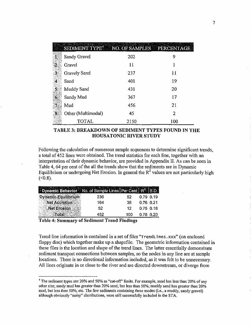
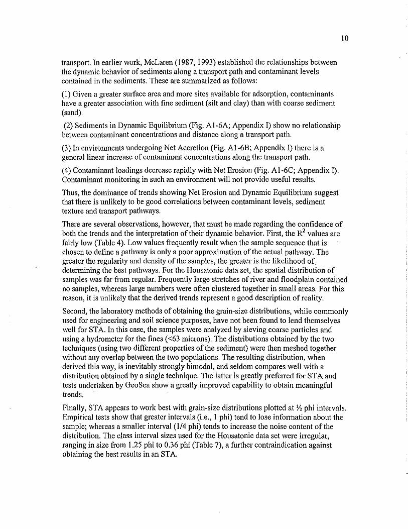
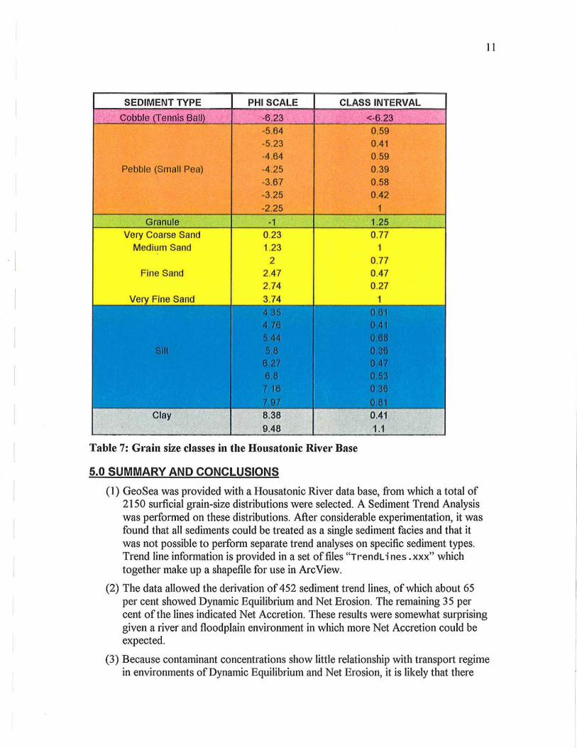

GeoSea Appendix I Page 2
11 Case A (Development of a lag deposit)
Consider a sedimentary deposit that has a grain-size distribution g(s) (Fig AI-I) If eroded the sediment that goes into transport has a new distribution r(s) which is derived from g(s) according to the function t(s) so that
r(s) = kmiddot g(s )t(s)
r(s ) or ()t s = kmiddotg()s
where g(sJ and r(sJ define the proportion of the sediment in the i1h grain-size class interval for each of the sediment distributions k is a scaling factor that normalizes r(s) so that
N
Lgt(s) = I 1=1
I thus k =--N-----shy
2 g(s )t(s) =1
With the removal ofr(s) from g(s) the remaining sediment (a lag) has a new distribution denoted by I(s) (Fig AI-I) where
I(s) =kmiddot g(s)[1- t(s)]
I(s) or t()s = ()
kmiddotg s
where t(s) = 1- t(s)
The function t(s) is defined as a sediment transfer function and is described in exactly the same manner as a grain-size probability function except that it is not normalized It may be thought of as a function that incorporates all sedimentary and dynamic processes that result in initial movement and transport of particular grain sizes
k is actually more complex than a simple normalizing function and its derivation and meaning is the subject of further research It appears to take into account the masses of sediment in the source and in transport and may be related to the relative strength of the transporting process
GeoSea Appendix I Page 3
[]-- t(s-4_r(_s_)
I 1-t(s)
I(s)
Figure AI-1 Sediment transport model to develop a lag deposit (see text for definition of terms)
Data from flume experiments show that distributions of transfer functions change from having a high negative skewness to being nearly symmetrical (although still negatively skewed) as the energy of the erodingtransporting process increases These two extremes in the shape of I(s) are termed low energy and high energy transfer functions respectively (Fig AI-2) The shape of I(s) is also dependent not only on changing energy levels of the process involved in erosion and transport but also on the initial distribution of the original bed material g(s) (Fig AI-I) The coarser g(s) is the less likely it is to be acted upon by a high energy transfer function Conversely the finer g(s) is the easier it becomes for a high energy transfer function to operate on it In other words the same process may be represented by a high energy transfer function when acting on fine sediments and by a low energy transfer function when acting on coarse sediments The terms high and low energy are therefore relative to the distribution ofg(s) rather than to the actual process responsible for erosion and transport
The fact that t(s) appears to be mainly a negatively skewed function results in r(s) the sediment in transport always becoming finer and more negatively skewed than g(s) The function i-I(s) (Fig AI-I) is therefore positively skewed with the result that I(s) the lag remaining after r(s) has been removed will always be coarser and more positively skewed than the original source sediment
If I(s) is applied to g(s) many times (ie n times where n is large) then the variance of both g(s) and I(s) will approach zero (ie sorting will become better) Depending on the initial distribution ofg(s) it is mathematically possible for variance to become greater before eventually decreasing In reality an increase in variance in the direction of transpOli is rarely observed
GeoSea Appendix I Page 4
Figure AI-2 Diagram showing the extremes in shape of transfer functions t(ltp)
Given two sediments whose distributions are ds) and dis) and dis) is coarser better sorted and more positively skewed than ds) it may be possible to conclude that dis) is a lag of ds) and that the two distributions were originally the same (Case A Table AIshyl)
12 Case B (Sediments becoming finer in the direction of transport)
Consider a sequence ofdeposits (ds) d2(s) dis)) that follows the direction of net sediment transport (Fig AI-3) Each deposit is derived from its corresponding sediment in transport according to the 3-box model shown in Figure AI-I Each dll(s) can be considered a lag of each rs) Thus ds) will be coarser better sorted and more positively skewed than rs) Similarly each rs) is acted upon by its corresponding fll(s) with the result that the sediment in transport becomes progressively finer better sorted and more negatively skewed Any two sequential deposits (eg dls) and d2(s) may be related to each other by a function X(s) so that
GeoSea Appendix I Page 5
d(s) = kA(s)X(s)
or X(s) = d2(s) k middotd(s)
Iwhere k = ----N----shy
L=dsJ X(s)
As illustrated in Figure AI-3 d2(s) can also be related to dls) by
kA(s)t(s)[I-t2(s)]()d 2 s = I-t ( ) s
=kA(s)X(s) (I)
where ()X s --
t(s)[I-t2(s)] I-t(s)
(2)
The functionX(s) combines the effects of two transfer functions tls) and t2(S) (Equation 2) It may also be considered as a transfer function in that it provides the statistical relationship between the two deposits and it incorporates all of the processes responsible for sediment erosion transport and deposition The distribution of the deposit dis) will therefore change relative to dls) according to the shape ofX(s) which in turn is derived from the combination of tls) and tis) as expressed in Equation 2 It is important to note thatX(s) can be derived from the distributions of the deposits dls) and d2(s) (Equation 1) and it provides the relative probability of any particular sized grain being eroded from db transported and deposited at d2
Using empirically derived t(s) functions it can be shown that when the energy level of the transporting process decreases in the direction of transport (ie tisJ lt tlsJ) and both are low energy functions (Fig AI-4) thenX(s) is always a negatively skewed distribution This will result in d2(s) becoming finer better sorted and more negatively skewed than dls) Therefore given two sediments (d l and d2) where dis) is finer better sorted and more negatively skewed than dls) it may be possible to conclude that the direction of sediment transport is from dl to d2 (Table AI-I)
GeoSea Appendix I Page 6
--- DIRECTION OF SEDIMENT TRANSPORT
Figure AI-3 Sediment transport model relating deposits in the direction of transport (see Appendix I for definition of terms)
13 Case C (Sediments becoming coarser in the direction oftransport)
In the event that ts) is a high energy function (Fig AI-2) and tisJ lt tsJ (ie energy is decreasing in the direction of transport) the result of Equation 2 will produce a positively skewed X(s) distribution Therefore dis) will become coarser better sorted and more positively skewed than dls) in the direction of transport (Fig AI-4) When these changes occur between two deposits it may be possible to conclude that the direction of transport is from dJ to d2 (Table AI-I)
l
GeoSea Appendix I Page 7
SORTING
+ MEAN
CASBC TfSIIlIlOddirectiooforOoarseoingSeoJimltamp
CASBR 1Toosport directiooforFining ampdimootamp
Figure AI-4 Changes in grain-size descriptors along transport paths
GeoSea Appendix I Page 8
TABLE AI-I Summary of the interpretations with respect to sediment transport trends when one deposit is compared to another
CASE
RELATIVE CHANGE IN GRAIN-SIZE DISTRIBUTION
BETWEEN DEPOSIT d2 AND DEPOSIT d INTERPRETATION
A Coarser Better sorted
More positively skewed
d2 is a lag of d No direction of transport can
be determined
B Finer Better sorted
More negatively skewed
(i) The direction of transport is from d to d2
(ii) The energy regime is decreasing in the direction
of transport (iii) 1 and 12 are low energy
transfer functions
C Coarser Better sorted
More positively skewed
(i) The direction of transport is from d to d2
(ii) The energy regime is decreasing in the direction
of transport (iii) 1 is a high energy
transfer function and 12 is a high or low energy transfer
function (Fig AI-5)
Sediment coarsening along a transport path will be limited by the ability of lis) to remain a high energy function As the deposits become coarser it will be less and less likely that the transport processes will maintain high energy characteristics With coarsening the transfer function will eventually revert to its low energy shape (Fig AI-2) with the result that the sediment must become finer again
Cases A and C produce identical grain-size changes between d and d2 (Table AI-) Generally however the geological interpretation of the environments being sampled will differentiate between the two Cases
GeoSea Appendix I Page 9
CASE B t2 lt t1 both low energy functions
X(qraquo (negative skew)
CASE C t2 lt t1 t1 is a high energy function t2 is high or low
t1 (high)
t2 (high)
Figure AI-5 Summary diagram oftl and t2 and corresponding X-distribution (Equation 2) for Cases Band C (Table AI-I)
20 METHOD TO DETERMINE TRANSPORT DIRECTION FROM GRAIN-SIZE DISTRIBUTIONS (SEDIMENT TREND ANALYSIS)
21 Uncertainties
The above model indicates that grain-size distributions will change in the direction of transport according to either Case B or Case C2 (Table AI-I Fig AI-4) Thus if any two
2 Case A which defines the development of a lag deposit is not used to determine a sediment transport direction There may be instances when a Case C transport direction is determined which in fact is not Case C transport but rather Case A For example in some Arctic environments sediments become progressively coarser better sorted and more positively skewed from deep to shallow water It is impossible
GeoSea Appendix I Page 10
samples (d and d2) are compared sequentially (ie at two locations within a sedimentary facies) and their distributions are found to change in the described manner the direction of net sediment transport may be inferred
A Sediment Trend Analysis attempts to determine the patterns of net sediment transpott over an area through the grain-size distributions of the sediments The sampled sediments are described in statistical terms (by the moment measures of mean sorting and skewness) and the basic underlying assumption is that processes causing sediment transport will affect the statistics of the sediments in a predictable way Following from this assumption the size frequency distributions of the sediments provide the data with which to search for patterns of net sediment transport
In reality perfect sequential changes along a transport path as determined by the model are rarely observed This is because ofa variety of uncertainties that may be introduced in sampling in the analytical technique to obtain grain-size distributions in the assumptions of the transport model and in the statistics used in describing the grain-size distributions These uncertainties may be summarized as follows
(I) The use ofthe log-normal distribution
Although sediments are typically described by a palticle weight distribution based on the log of the grain-size (ie the phi scale where palticle diameter in mm = 2~) there is in fact no way to determine the best descriptor for all sediments The log-normal distribution has been found useful in practice since it appears to highlight important features of naturally occurring sediments Bias can however be introduced in the choice of distribution For example the mean of the distribution in phi space is not equal to the mean of the distribution in linear space Using the moment measures (mean variance and skewness) may highlight important features and suppress those that are unimportant however information will also be lost There is no way to detelmine if the lost information is significant (Bowles and McLaren 1985)
Whatever method is used to describe the sediments the trend analysis requires the above model which demonstrates that transport processes will change the moment measures of sediments in a predictable way It is hoped that future research may be able to address the possible benefits of using other distributions (eg the log hyperbolic distribution Hartmann and Christiansen 1992)
to suppose that there is a high energy transport fumction operating on the deep water sediments resulting in Case C transport towards the shoreline In this enviroment ice action and currents result in the winnowing of the finer size fractions as the water shallows Thus Case A indicating the development of a lag is the accepted Case rather than Case C As stated earlier a geological interpretation may be required to differentiate between the development of a lag (Case A) and a genuine transport pathway (Case C)
GeoSea Appendix I Page 11
(2) Assumptions in the transport model
In providing a mathematical proof for the transport model used in the Sediment Trend Analysis (McLaren and Bowles 1985) a basic assumption is made that smaller grains are more easily transported than larger grains As seen in the transfer functions obtained from flume experiments (Fig AI-2) this assumption is not strictly true The curves monotonically increase over only a portion of the available grain sizes before returning to zero Factors such as shielding whereby the presence of larger grains may impede the transport of smaller grains or the decreasing ability of the eroding process to carry additional fines with increasing load demonstrate that the transport process is a complicated function related to the sediment distribution and the strength of the erosion process
(3) Temporal fluctuations
Sediment samples may comprise the effects of several transport processes It is assumed that what is sampled is the average of all the transport processes affecting the sample site The average transport process may not conform to the transport model developed for a single transport process
In a Sediment Trend Analysis it is assumed that a sample provides a representation of a specific sediment type (or facies) There is no direct time connotation nor does the depth to which the sample was taken contain any significance provided that the sample does in fact accurately represent the facies For example dJ may be a sample of a facies that represents an accumulation over several tidal cycles and d2 represents several years of deposition The trend analysis simply provides the sedimentological relationship between the two (see McLaren 1981 for a more detailed discussion of sampling) The possibility also exists that different samples may result from a different suite oftransportevents
(4) Sample spacing
Sample sites may be too far apart to detect relevant transport processes With increasing distance between sample locations there is an increasing possibility of collecting sediments unrelated by transport (Le different facies) Sample sites placed X m apart can only be reliable to detect transport processes with a spatial scale of2X m or more Transport processes with smaller spatial scales may appear as noise or spurious signals
In practice selection of a suitable sample spacing takes into account (1) the number of sedimentological environments likely to be encountered (2) the desired spatial scale of the sediment trends and (3) the geographic shape of the study area (see below for fUilher discussion of sample spacing)
(5) Random environmental uncertainties
All samples will be affected by random errors These may include unpredictable fluctuations in the depositional environment the effects of sampling and sub-sampling a representative sediment population and random measurement errors
GeoSea Appendix I Page 2
22 The use of the Z-score statistic
Given the above list of complicating factors that introduce uncertainties in establishing the net patterns of transport it is rare to find sequences of samples whose distributions change exactly according to Figure AI-4 One approach that appears to be successful in determiniIig trends is a simple statistical method whereby the Case (Table AI-) is determined among all possible sample pairs contained in a specified sequence Given a sequence of n samples there are n - n directionally orientated pairs that may exhibit a
2 transport trend in one direction and an equal number ofpairs in the opposite direction When any two samples are compared with respect to their distributions the mean may become finer (F) or coarser (C) the sorting may become better (B) or poorer (P) and the skewness may become more positive (+) or more negative (-) These three parameters provide 8 possible combinations (Table AI-2)
TABLE AI-2 All possible combinations of grain-size parameters th t b ta may occur e veen an t d tvo epOSl s
1 2 3 4
Mean F C F F Sorting B B P B
Skewness - - - +
5 6 7 8
Mean C F C C Sorting P P B P
Skewness + + + -
Case B (Table AI-I) Case A or C (Table AI-I)
In Sediment Trend Analysis we postulate that a certain relationship exists among the set of n samples and that this relationship is evidenced by paliicular changes in sediment size descriptors between pairs of samples Then the number of pairs for which the trend relationship occurs should exceed the number of pairs that would be expected to occur at random by a sufficient amount for us to state confidently that the trend relationship exists Suppose the probability of any trend existing between any pair of samples if the trend relationships were established randomly is p Since there are 8 possible trend relationships among 3 sediment descriptors and we assume that each of these is equally likely to occur the value ofp is set at 0125
GeoSea Appendix I Page 13
To determine if the number of occurrences that a particular Case exceeds the random probability of 0125 the following two hypotheses are tested
Ho plt0125 and there is no preferred direction and HI pgt0125 and transport is occurring in the prefel1ed direction
Using the Z-score statistic in a one-tailed test (Spiegel 1961) HI is accepted if
Z = ~)1645 (005 level of significance)Nqp
or )233 (001 level of significance)
where x is the observed number of pairs representing a particular Case in one of the two opposing directions and N is the total number of possible unidirectional pairs given by
2
n -n The number of samples in the sequence is np is 0125 and q is 10 - p = 0875 2
The Z statistic is considered valid for N)30 (ie a large sample) Thus for this application a suite of 8 or 9 samples is the minimum required to evaluate adequately a transport direction
30 DERIVATION OF SEDIMENT TRANSPORT PATHWAYS
From the above it is seen that a variety ofuncertainties may preclude obtaining a perfect sequence ofprogressive changes in grain-size distributions from sediment samples that follow a specific transport pathway (Fig AI-4) In using the Z-score statistic however a transport trend may be detennined whereby all possible pairs in a sample sequence are compared with each other When either a Case B or Case C trend exceeds random probability within the chosen sample sequence the direction of net sediment transpOli can be inferred In using the Z-score statistic a minimum of 9 samples should be used which indicates that iftranspOli pathways are to be determined over a specific area a minimum grid of9 X 9 samples is required (ie 81 samples) As suggested above the grid spacing must be compatible with the area under study and take into account the number of sedimentological environments likely to be involved the geographic shape of the study area and the desired statistical certainty of the pathways For practical purposes it has been found that for regional studies in open ocean environments sample spacing should not exceed 1 km in estuaries spacing should be reduced to 500 m For site specific studies (eg to determine the transport regime for a single marina) sample spacing will be reduced so that a minimum number of samples can be taken to ensure an adequate coverage (ie 9 X 9 samples) Experience has also shown that extra samples should be taken over sites of specific interest (eg dredged material disposal sites) and should the regular grid be insufficient from specific bathymetric features (eg bars and channels)
In determining transport patterns over an area it is useful to draw an analogy with communication systems In the latter infonnation is transmitted to a distant location where a signal is received containing both the desired information as well as noise The
GeoSea Appendix I Page 14
receiver must extract the information from the noisy signal In theory the information can be recovered by simply subtracting the noise from the signal an approach that works well in communications systems because the nature of both the information and the noise is well known
In sedimentary systems the information is the direction of net sediment transport and the received signal is the grain-size distributions of the sediment samples The goal of a Sediment Trend Analysis is to extract the information from the noisy signal which in this case may be difficult because neither the nature of the information nor the noise is known
There is however another approach that draws from communications theory In some communications systems the information from many sources is combined into one signal which from a statistical viewpoint is nothing but noise To extract specific infotmation the receiver assumes that the information is present and determines if that assumption is consistent with the received signaJ3
The same approach may be used in a Sediment Trend Analysis as follows (i) assume the direction of sediment transport over an area containing many sample sites (ii) from this assumption predict the sediment trend that should appear along a particular sequence of samples (iii) compare the prediction with the actual trend that is derived from the selected samples (iv) modifY the assumed transport direction and repeat the comparison until the best fit is achieved
The impOliant feature of this approach is the use of many sample sites to detect a transport direction This effectively reduces the level of noise The principal difficulty is that the number of possible pathways in a given area may be too large to mechanize the technique or to try them all As a result the choosing of trial transport directions has as yet not been analytically codified (research is on-going to do this) At present the selection of trial directions is undertaken initially at random although the term random is used loosely in that it is not strictly possible to remove the element of human decisionshymaking entirely For example a first look at the possible transport pathways may encompass all north-south or all east-west directions As familiarity with the data increases exploration for trends becomes less and less random The number of trial trends becomes reduced to a manageable level through both experience and the use of additional information (usually the bathymetry and morphology of the area under study) Following from the communications analogy when a final and coherent pattern of transport pathways is obtained that encompasses all or nearly all of the samples the assumption that there is information (the transport pathways) contained in the signal (the grain-size distributions) has been verified despite the inability to define accurately all the uncetiainties that may be present
3This is a process referred to as Code Division MUltiplexing
GeoSea Appendix I Page 15
40 THE USE OF R2
In order to assess the validity of any transport line we use the Z-score and an additional statistic the linear correlation coefficient R2 defined as
The value of R2 can range from 0 to 1 The definition of R2 is based on the use of a model to relate a dependent parameter y to one or more independent parameters (x tX2) In our case the model used is a linear one which can be written as
y =ao +a middotx +a middotx
The data (Yx tx2) are grain-size distribution statistics and the parameters (aoa ta2) are estimated from the data using a least-squares criterion The dependent parameter is defined as the skewness and the independent parameters are the mean size and the sorting We make an implicit assumption that grain size samples making up a transport line if plotted in skewnesssortingmean space (as in Fig AI-4) would tend to be clustered along a straight line The slopes of the straight line which are the fitted parameters would depend on the type of transport (fining or coarsening) While there is no theoretical reason to expect a linear relationship among the three descriptors there is also no theory predicting any other kind of relationship so using the principle of Occams Raz0l4 we choose the simplest available relationship as our model High values of R2 (08 or greater) together with a significantly high value ofthe Z-score give us confidence in the validity of the transport line
A low R2 may occur even when a trend is statistically acceptable for the following reasons (i) sediments on an assumed transport path are in reality from different facies and valid trend statistics occurred accidentally (ii) the sediments are from a single facies but the chosen sequence is only a poor approximation of the actual transport path and (iii) extraneous sediments have been introduced into the natural transport regime as in the case of dredged material disposal R2 therefore is assessed qualitatively and when low statistically acceptable trends must be treated with caution
50 INTERPRETATION OF THE X-DISTRIBUTION
The shape of the X-distribution is important in defining the type of transport OCCUlTing along a line (erosion accretion total deposition etc) and thus the computation ofX is important Let us suppose that we have defined a transport line containing N sourcedeposit (dd2) pairs Then we defineXas
40ccams Razor Entities ought not to be mUltiplied except from necessity (Occam 14th Century philosopher died 1349)
GeoSea Appendix I Page 16
X(s) = f ~dI(S) 1=1 d l i (s)
Often d2 in one pair is d in another pair and vice versa Mean values of d2 and d are computed through
Note that we do not defineXas the quotient of the mean value ofd2 divided by the mean value of d even though the results of the two computations are often almost identical For ease of comparison d d2 and X are normalized before plotting in reports although there is no reason to expect that the integral of the X distribution should be unity
X(s) may be thought of as a function that describes the relative probability of each particle being removed from d and deposited at d2bull It must be emphasized that the processes responsible for the transpOli of particles from d to d2 are unknown they may in one environment be breaking waves in another tidal residual currents and in still another incorporate the effects of bioturbation
Examination ofXmiddotdistributions from a large number of different environments has shown that five basic shapes are most common when compared to the distributions of the deposits dis) and dis) (Fig AImiddot6) These are as follows
(1) Dynamic Equilibrium The shape of the Xmiddotdistributions closely resembles dis) and dis) The relative probability of grains being transported therefore is a similar distribution to the actual deposits Thus the probability of finding a particular sized grain in the deposit is equal to the probability of its transport and remiddotdeposition (ie there must be a grain by grain replacement along the transport path) The bed is neither accreting nor eroding and is therefore in dynamic equilibrium
An Xmiddotdistribution signifying dynamic equilibrium may be found in either Case B or Case C transport suggesting that there is fine balance between erosion and accretion Often when such environments are determined both Case B and Case C trends may be significant along the selected sample sequence This is referred to as a Mixed Case and when this occurs it is believed that the transport regime is also approaching a state of dynamic equilibrium
(2) Net Accretion The shapes of the three distributions are similar but the mode of X is finer than the modes ofdis) and dis) The mode ofX may be thought of as the size that is the most easily transported Because the modes of the deposits are coarser than X these sizes are more readily deposited than transported The bed therefore must be in a state of net accretion Net accretion can only be seen in Case B transpOli
(3) Net Erosion Again the shapes of the three distributions are similar but the mode of X is coarser than the dis) and dis) modes This is the reverse of net accretion where the size
GeoSea Appendix I Page 17
most easily transported is coarser than the deposits As result the deposits are undergoing erosion along the transport path Net erosion can only be seen in Case C transport
(4) Total Deposition I Regardless of the shapes of dis) and d2(s) the X-distribution more or less increases monotonically over the complete size range of the deposits Sediment must fine in the direction of transport (Case B) however the bed is no longer mobile Rather it is accreting under a rain of sediment that fines with distance from source Once deposited there is no further transport The OCCUl1ence of total deposition is usually confined to cohesive muddy sediments
(5) Total Deposition II (Horizontal X-Distributions) Occul1ing only in extremely fine sediments when the mean grain-size is very fine silt or clay the X-distribution may be essentially horizontal Such sediments are usually found far from their source and the horizontal nature of the X-distribution suggests that their deposition is no longer related strictly to size-sorting In other words there is now an equal probability of all sizes being deposited This form of the X-distribution was first observed in the muddy deposits of a British Columbia fjord and is described in McLaren Cretney et aI 1993 Because the trends occur in very fine sediments where any changes in the distributions are extremely small horizontal X-distributions may be found in both Case B and Case C trends
GeoSea Appendix I Page 18
A Dynamlc Equilibrium B Net Accretion
~ ~ ==~ -xI
I
C Net Erosion D Total Deposition I
E Total Deposition II (horizontal X -function)
~ lt- I-----~IIr-----~--------~------___
Figure AI-6 Summary ofthe interpretations given to the shapes ofX-distributions relative to the DJ and D2 deposits
GeoSea Appendix I Page 19
60 REFERENCES
Bowles D and McLaren P 1985 Optimal configuration and information content of sets of frequency distributions - discussion Journal of Sedimentary Petrology V55 931-933
Hartmann D and Christiansen C 1992 The hyperbolic shape triangle as a tool for discriminating populations of sediment samples of closely connected origin Sedimentology V39 697-708
McLaren P and Bowles D 1985 The effects of sediment transport on grain-size distributions Journal of Sedimentary Petrology V55 457-470
McLaren P Cretney WJ and Powys R 1993 Sediment pathways in a British Columbia fjord and their relationship with particle-associated contaminants Journal of Coastal Research V9 1026-1043
McLaren P 1981 An interpretation of trends in grain-size measures Journal of Sedimentary Petrology V51 611-624
- barcodetext SDMS DocID 512707
- barcode 512707
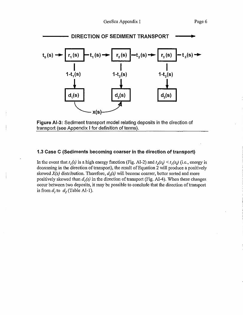
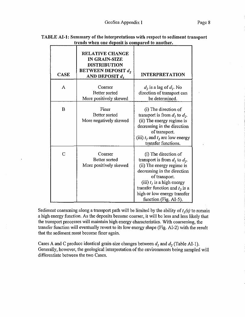
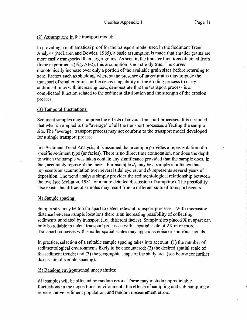