scaling implementation of a tension recti cation algorithm...

Scientia Iranica E (2014) 21(3), 980{987

Sharif University of TechnologyScientia Iranica

Transactions E: Industrial Engineeringwww.scientiairanica.com

Scaling implementation of a tension recti�cationalgorithm to solve the feasible di�erential problem

M. Ghiyasvand�

Department of Mathematics, Faculty of Science, Bu-Ali Sina University, Hamedan, Iran.

Received 19 May 2012; received in revised form 16 November 2012; accepted 8 June 2013

KEYWORDSOperations research;Network ows;The feasibledi�erential problem;Tension recti�cationalgorithm;Scalingimplementation.

Abstract. The feasible di�erential problem is solved using a tension recti�cationalgorithm. In this paper, we present a scaling implementation of a tension recti�cationalgorithm. Let n;m;U denote the number of nodes, number of arcs, and maximum arccapacity value of an arc, respectively. Our implementation runs in O(mn logU), whichis O(mn log n) under the similarity assumption. The tension recti�cation algorithm runsin O(m2) time, so, our implementation is an improvement if n log n < m. Another meritof our algorithm is that, in cases where the feasible di�erential problem does not havea solution, it presents some information that is useful to the modeler in estimating themaximum cost of adjusting the network.c 2014 Sharif University of Technology. All rights reserved.

1. Introduction

The �rst theoretical studies on tension were discussedby Berge and Ghouila-Houri [1,2] at the beginningof the 1960s. In 1971, Pla [3] presented an out ofkilter algorithm to solve the minimum cost tensionproblem. Hajiat [4] showed that Pla's algorithm isnot polynomial using a graph family fTn; n � 2g onwhich it runs necessarily in an exponential number ofiterations, namely, 2n+2n�1 +2n�2�2 calls to a linearlabeling process. Hamacher [5] developed two pseudo-polynomial time algorithms in 1985: negative cutand shortest augmenting cut algorithms. Other non-polynomial algorithms were given by Rockafellar [6].Polynomial time algorithms to solve the minimum costtension problem have been presented by Hadjiat andMaurras [7] and Ghiyasvand [8,9]. Piecewise linearand convex costs of the problem and inverse tensionproblems have been discussed in [10-14].

Let D = (N;A) be a connected digraph withvertex set, N , containing n vertices, and arc set, A,containing m arcs. We denote an arc from node i to

*. E-mail address: [email protected] (M. Ghiyasvand)

node j by (i; j). Let RA (resp. RN ) be a collection ofall orderedm-tuples (resp. n-tuples) of real numbers onset A (resp. N). A vector � 2 RA is a tension on graphG with a potential � 2 RN , such that �ij = �j��i, foreach (i; j) 2 A. Each arc, (i; j) 2 A, has a capacity, uij ,that denotes the maximum amount of �ij on the arc anda lower bound lij that denotes the minimum amountof �ij on the arc. Tension � is called a feasible tensionif lij � �ij � uij , for each (i; j) 2 A. The feasibledi�erential problem determines a feasible tension (if itexists).

A cycle, C, in a directed graph is a sequencei1; i2; : : : ; ik of distinct nodes of N , such that either(ir ! ir+1) 2 A (a forward arc in C) or (ir+1 !ir) 2 A (a backward arc in C) for r = 1; 2; : : : ; k (wherewe interpret ik+1 as i1). It is obvious that tension isarc-weighting, having a zero sum on every cycle of thegraph, so, for each cycle, C, we have:X

(i;j)2C+

�ij � X(i;j)2C�

�ij = 0; (1)

where C+ and C� are the forward and backward arcsof the cycle, respectively. For a given cycle, C, de�ne:

M. Ghiyasvand/Scientia Iranica, Transactions E: Industrial Engineering 21 (2014) 980{987 981

d+(C) =X

(i;j)2C+

uij � X(i;j)2C�

lij : (2)

The next theorem presents a necessary and su�cientcondition to conclude that the feasible di�erentialproblem has a feasible tension.

Theorem 1 (Feasible di�erential theorem [6,page 193]). The feasible di�erential problem has afeasible tension if and only if d+(C) � 0 for each cycle,C. �

The feasible di�erential problem can be solvedusing a tension recti�cation algorithm [6, page 203-5,and 15, page 70]. The tension recti�cation algorithmruns in O(m2) time ([6], page 205, line 20). When thefeasible di�erential problem does not have a feasibletension, this algorithm only computes cycle C withd+(C) < 0.

In this paper, we �rst present a scaling idea tosolve the feasible di�erential problem, then a scalingimplementation of the tension recti�cation algorithmis presented, which is a new method for solving theproblem. Our algorithm runs in O (mn logU) time,where U is the maximum arc capacity value of an arc.

To avoid systematic underestimation of runningtime, in comparing two running times, sometimes, itwill be assumed that the bound, U , is polynomialbounded in n, namely, U = O(nk), for some constantk [16]. This assumption is called as the similarityassumption [17, page 60]. Thus, under the similarityassumption [16], our algorithm runs in O(mn log n),which is an improvement if n logn < m (in comparisonwith the tension recti�cation algorithm [6,15]).

In cases where the feasible di�erential problemdoes not have a feasible tension, our algorithm not onlypresents a cycle, C, with d+(C) < 0, but also givessome information so that the modeler can estimate themaximum cost of repairing the network in order to havea network with a feasible tension.

This paper consists of three sections in additionto the introduction. Section 2 presents a brief outlineof the tension recti�cation algorithm. A scaling im-plementation of the tension recti�cation algorithm isshown in Section 3. Finally, Section 4 presents a fasterimplementation of the algorithm described in Section 3.

2. The tension recti�cation algorithm

In this section, a brief outline of the tension recti�ca-tion algorithm [6,15] is presented. Given an arbitrarypotential, �, and its tension �, let:

A+ = f(i; j) 2 Aj�ij < lijg;A� = f(i; j) 2 Aj�ij > uijg:

If A+ = � = A�, tension � is feasible. Otherwise

any arc (r; s) 2 A+ [ A� is selected. Then, Minty'sLemma [18] is applied using the following painting ofthe arcs (i; j) 2 A: red (if lij < �ij < uij), black(if �ij � lij and �ij < uij), white (if �ij � uij and�ij > lij), and green (if lij = �ij = uij). It is obviousthat (r; s) will be black or white.

If the outcome of Minty's lemma is a cycle, C,containing (r; s) terminate; this cycle has d+(C) < 0.Otherwise, the outcome is a set, W , of nodes, suchthat (r; s) 2 (W;W ) = f(i; j) j i 2 W , j 62 Wg or(r; s) 2 (W;W ) = f(i; j) j i 62 W , j 2 Wg, whereW = N �W . In this case, the value, �, is computedas follows:

� =

8><>:uij � �ij ; if (i; j) 2 (W;W );�ij � lij ; if (i; j) 2 (W;W );�; otherwise;

where:

� =

(lrs � �rs; if (r; s) 2 A+;�rs � urs; if (r; s) 2 A�:

Then, the updated potentials are:

�0i =

(�i; if i 2W;�i + �; if i 2W:

The tension recti�cation algorithm repeats with �0 inwhich, after a �nite number of iterations, arc (r; s) is�nally removed from A+[A�. These operations repeatfor each arc in A+ [A� and the algorithm can be runin O(jAj(jA+j+ jA�j)) � O(jAj2) = O(m2) time.

2.1. Application of the feasible di�erentialproblem

The minimum cost tension problem appears in manyapplications (Rockafellar [6, Chapter 7F]) concerningnetworks, such as timing of events, location of facilities,shared cost problems, and so on. Let cij denote thecost on arc (i; j). the minimum cost tension problemdetermines a feasible tension with minimum cost. Theminimum cost tension problem is de�ned as follows:

minX

(i;j)2Acij�ij

s.t. � is a feasible tension.

All minimum cost tension algorithms [2-5,7-9,19,20]start with a feasible tension. Thus, before solving theminimum cost tension problem, the feasible di�erentialproblem should be solved in order to �nd a feasibletension, or to diagnose that the problem does not havea feasible tension.

982 M. Ghiyasvand/Scientia Iranica, Transactions E: Industrial Engineering 21 (2014) 980{987

3. A scaling implementation of the tensionrecti�cation algorithm

In this section, a scaling implementation of the tensionrecti�cation algorithm is presented. Given a � > 0,we de�ne tension � as a �-feasible tension if, for each(i; j) 2 A:

lij � � < �ij < uij + �: (3)

Our algorithm starts out with � large and drive �toward zero. In each phase, the algorithm tries to �nda �-feasible tension using the input 2�-feasible tension.The following lemma says that � need not start out toobig and end up too small.

Theorem 2. � = 0 is a (U + 1)-feasible tension.Moreover, if l and u are integer and there exists a �-feasible tension �, such that � � 1=m, then, the feasibledi�erential problem has a solution.

Proof. By U = maxfjlij j; juij j j for each(i; j) 2 Ag,we get lij � U � 0 � uij + U (for each arc i ! j),which means:lij � (U + 1) < 0 < uij + (U + 1): (4)

Let � = 0, which concludes � = 0 is a tension and, byInequality (4), is a (U + 1)-feasible tension.

Now, considering cycle C, by Eqs. (1) and (2), weget:

�d+(C) =X

(i;j)2C+

(�ij � uij) +X

(i;j)2C�(lij � �ij):

Tension � is �-feasible, so, by Inequality (3), we have:

�d+(C) <X

(i;j)2C+)

� +X

(i;j)2C�� m�:

Thus, if we have a �-feasible tension with � � 1=m,then, d+(C) > �m� � �1. Since l and u are integer,d+(C) is integer too, which means d+(C) � 0: Cycle Cis arbitrary, so, Theorem 1 concludes that the feasibledi�erential problem has a solution. �

Thus, our algorithm starts with � = U and x = 0.In each phase, the input is a 2�-feasible tension andthe output is a �-feasible tension. By Theorem 2, thealgorithm runs in O(log(nU)) phases. To explain aphase, we need the following de�nition.

De�nition 1. Given a tension, �, for each node, i 2N , value �(i) is de�ned by the following:

�(i) = max

8>>><>>>:lij � �ij ; for each outgoing arc

(i; j) of node i;�ri � uri; for each incoming arc

(r; i) of node i:

(5)

The next conclusion is a result of de�nitions, which

Figure 1. If �ij � lij , then (i; j) is in the set �. Iflij < �ij < uij , then (i; j) is in the set �. Also, if �ij � uij ,then (i; j) is in the set r.

Figure 2. If �ji > uji or �ij < uij , then �(i) = �(i) [ fjg.

presents a relationship among �(i)'s and �-feasibletension.

Conclusion 1. Given a tension, �. For each i 2 N ,�(i) < � if and only if lij � � < �ij < uij + �, for each(i; j) 2 A.

Using Conclusion 1, we can work on �(i)'s in orderto have a �-feasible tension. For this purpose, we needthe following de�nitions. Sets r, � and � are de�nedin the following way (Figure 1):

� = f(i; j) 2 A j lij � 2� < xij � lijg;r = f(i; j) 2 A j uij � xij < uij + 2�g;� = f(i; j) 2 A j lij < xij < uijg:

Let F (�) = fi 2 N j � � �(i) < 2�g, so, there isa relationship among sets F (�);� and r, which is asfollows.

Conclusion 2. If i 2 F (�), then, at least one of thefollowing occurs:

a) There is at least one outgoing arc (i; j) of node iwith �ij < lij .

b) There is at least one incoming arc (r; i) of node iwith �ri > uri.

Considering a node i 2 F (�), using Conclusion 2, wede�ne node �(i) as follows.

De�nition 2. For each outgoing arc (i; j) of nodei with �ij < lij (resp. incoming arc (r; i) of node iwith �ri > uri), let �(i) = �(i) [ fjg (resp. �(i) =�(i) [ frg), see Figure 2(a) and (b).

In each phase of our algorithm, a 2�-feasibletension, �, should be changed to a �-feasible tension, �0.If F (�) = �, then � is �-feasible tension, and the currentphase is �nished. Otherwise, it selects a node, i 2 F (�),and labels the nodes using the labeling procedure (i)presented in Algorithm 1. The set of labeled nodes at


Algorithm 1. The labeling procedure.

Algorithm 2. The scaling tension recti�cation algorithm.

the end of the labeling procedure (i) is de�ned by W .The following theorem shows how it can be diagnosedwhen the feasible di�erential problem does not have asolution.

Theorem 3. Let W be the set of labeled nodes at theend of the labeling procedure (i). If �(i) \ W 6= �,then, the feasible di�erential problem does not have asolution.

Proof. By the labeling procedure (i), when �(i)\W 6=�, there is a cycle, C, such that:

(i; j) 2 r; for each (i; j) 2 C+;

(i; j) 2 �; for each (i; j) 2 C�:Thus, we get:X

(i;j)2C+

uij � X(i;j)2C+

�ij ; (6)

and:

X(i;j)2C�

�ij � X(i;j)2C�

lij : (7)

The arc (i; j) or (j; i) with j 2 �(i) is in cycle C, so, byFigure 2, one of Inequalities (5) or (6) is strict. Thus,by Eq. (1), we have:X

(i;j)2C+

uij � X(i;j)2C�

lij < 0;

which means, using Theorem 1, the feasible di�erentialproblem does not have a solution. �

Using Theorem 2 and Conclusion 2, we get thefollowing conclusion, which shows how the feasibilityof the feasible di�erential problem can be diagnosed.

Conclusion 3. If l and u are integer and F (�) =�, such that � � 1=m, then, the feasible di�erentialproblem has a solution.

Algorithm 2 presents our method, which selects anode, i 2 F (�), then removes node i from set F (�) by


adjusting �i' s and �ij 's, as follows.

�0i =

(�i � �; if i 2W;�i; if i 2W:

(8)

By Eq. (7), �ij 's are changed according to:

�0ij =

8><>:�ij + �; if (i; j) 2 (W;W );�ij � �; if (i; j) 2 (W;W );�ij ; otherwise:

(9)

The next lemma proves that node i leaves set F (�)using Eqs. (7) and (8).

Lemma 1. Suppose that �(i)\W 6= at the end of thelabeling procedure (i). After adjusting �i' s and �ij 's,according to Eqs. (7) and (8), we have �(i) < �.

Proof. Let W = N �W . At the end of the labelingprocedure (i), we have (Figure 3):(i; j) 2 r; for each outgoing arc (i; j) of node i

with j 2W ,(r; i) 2 �; for each incoming arc (r; i) of node i

with r 2W ,(i; q) 2 � or �; for each outgoing arc (i; q) of node i

with q 2W ,(p; i) 2 r or �; for each incoming arc (p; i) of node i

with p 2W .We consider the following cases in order to com-

pute �(i), with regard to �0, computed by Eq. (8):

(i) The outgoing arcs of node i.(i-1) If (i; j) is an outgoing arc of node i with j 2W ,

then, by Figure 3, (i; j) 2 r, so, we get uij � �ij .By Eq. (8), �0ij = �ij , which means by lij � uij ,lij � �0ij � 0 < �.

(i-2) If (i; q) is an outgoing arc of node i with q 2W , then, by Figure 3, (i; q) 2 � or �, so, byFigure 1, we have liq � 2� < �iq < uiq. ByEq. (8), �0iq = �iq + �, so, by Figure 1, liq � � <�0iq < uiq + �, which means liq � �0iq < �.

Figure 3. After labeling procedure, for each(i; q) 2 (W;W ), we have (i; q) 2 � [ �. Also, for each(p; i) 2 (W;W ), we have (p; i) 2 r [ �.

(ii) The incoming arcs of node i.(ii-1) If (r; i) is an incoming arc of node i with r 2W ,

then, by Figure 3, (r; i) 2 �, so, we get �ri � lri.By Eq. (8), �0ri = �ri, which means, by lri � uri,�0ri � uri � 0 < �.

(ii-2) If (p; i) is an incoming arc of node i with p 2W , then, by Figure 3, (p; i) 2 r or �, so, byFigure 1, we have lpi < �pi < upi + 2�. ByEq. (8), �0pi = �pi � �, so, by Figure 1, lpi � � <�pi < upi + �, which means �pi � upi < �.

By De�nition 1 and cases (i-1),(i-2), (ii-1), and(ii-2), we get �(i) < �. �

Hence, by Lemma 1, node i leaves F (�). In orderto show that a phase �nishes after �nite iterations, weprove that the method does not enter a new node toset F (�).

Lemma 2. After adjusting �i' s and �ij 's, accordingto Eqs. (7) and (8), a new node does not add to setF (�).

Proof. By Eq. (8), �ij is changed if (i; j) 2 (W;W ) or(i; j) 2 (W;W ). Thus, we consider the following twocases:

Case-1. j 2W with at least oneincoming arc of nodej (Figure 4).

Case (1-1). If (i; j) is an incoming arc of node j withi 2 W , then, by Figure 4, (i; j) 2 � or �, so, we get�ij < uij . By Eq. (8), �0ij = �ij + �, so �0ij < uij + �,which means �0ij � uij < �. Thus, by De�nition 1, ifnode j is not in F (�), then, by adjusting �ij , accordingto Eq. (8), node j will not be added to set F (�).

Case (1-2). If (j; r) is an outgoing arc of node j withr 2 W , then, by Figure 4, (j; r) 2 r or �, so, we get�jr > ljr. By Eq. (8), �0jr = �jr � �, so, �0jr > ljr � �,which means ljr � �0jr < �. Thus, by De�nition 1, ifnode j is not in F (�), then, by adjusting �jr accordingto Eq. (8), node j will not be added to set F (�).

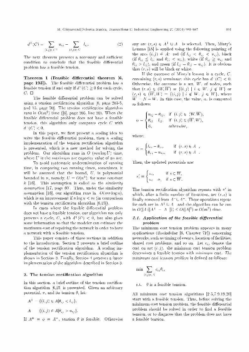
Case-2. i 2W with at least one outgoing arc of nodei (Figure 5).

Figure 4. The position of node j 2W with at least oneincoming arc of node j.


Figure 5. The position of node i 2W with at least oneoutgoing arc of node i.

Using Figures 3 and 5 and cases (i-2) and (ii-2) inthe proof of Lemma 1, if node i is not in F (�), then,by adjusting �ij 's, according to Eq. (8), node i will notbe added to set F (�). �

The next theorem computes the running time ofthe algorithm.

Theorem 4. The scaling tension recti�cation algo-rithm runs in O(mn log(nU)) time.

Proof. Using Theorem 2, the number of phases isO(log(mU)) = O(log(nU)). Each phase, for a given� > 0, �nishes, if F (�) = �. The algorithm selectsa node, i 2 F (�), and changes it to �(i) < � usingEqs. (7) and (8), which takes O(m). By Lemma 2,during a phase, no new node will be added to F (�),so, each phase needs jF (�)j � n iterations. Thus, eachphase runs in O(mn). �

Now, we show how the information of our algo-rithm is used to estimate maximum cost for repairingthe network in order to have a feasible tension.

Theorem 5. For a given � and i 2 F (�), if �(i)[W 6=�, then, the network can be repaired by, at most, 2m�changes in bounds in order to have a feasible tension.

Proof. �(i) [ W 6= � says the feasible di�erentialproblem does not have a feasible tension. Usingthe method of the algorithm, a 2�-feasible tension iscomputed in the last phase. Thus, we have a tension, �,with lij�2� < �ij < uij+2� (for each (i; j) 2 A), whichmeans that m(2�) is an upper bound on the number ofchanges in bounds (increasing uij 's or decreasing lij 'sby 2�), so that � be a feasible tension. �

4. Reducing the number of phases to O(log U)and �nding a feasible tension

At the end of Algorithm 2, we only can diagnose if thefeasible di�erential problem has a solution, but do not�nd a feasible solution. In this section, we reduce thenumber of phases to O(log U) and compute a feasiblesolution (if it exists). Let U = 2blogUc+1, so, U >U + 1, which means, by Theorem 2, � = 0 is a U -feasible tension.

Lemma 3. Let l and u be integer. Supposing thatthe starting � is � = U , then:

a) If there is a 1-feasible tension, then the feasibledi�erential problem has a solution.

b) Each 1-feasible tension is a feasible tension.

Proof. The starting values are � = 2blogUc+1, �ij = 0(for each (i; j) 2 A), and �i = 0 (for each i 2 N).Thus, initially, � is integer and a multiplier of 2. In eachiteration, � is reduced to �=2, which means the valuesof all �'s are integer if � � 1. During each iteration,the values of �i's and �ij 's are updated by Eqs. (7) and(8), so, they are integer if � � 1.

Supposing that we have a 1-feasible tension, �, so,lij � 1 < �ij < uij + 1, for each (i; j) 2 A. Thus, foreach (i; j) 2 A, we get:

uij��ij > �1) uij � �ij � 0

(because uij � �ij is integer);

�ij�lij > �1) �ij � lij � 0

(because �ij � lij is integer):

Therefore, lij � �ij � uij , for each (i; j) 2 A, whichmeans each 1-feasible tension is a feasible tension. �

The next theorem shows that the algorithm canbe run in O(mn logU) time using Lemma 3.

Theorem 6. If the scaling tension recti�cation algo-rithm starts with � = U , then, it runs in O(mn logU)time.

Proof. By Lemma 3, each 1-feasible tension is afeasible tension, so, the number of phases is O(logU) =O(logU). By the proof of Theorem 4, each phase runsin O(mn). �

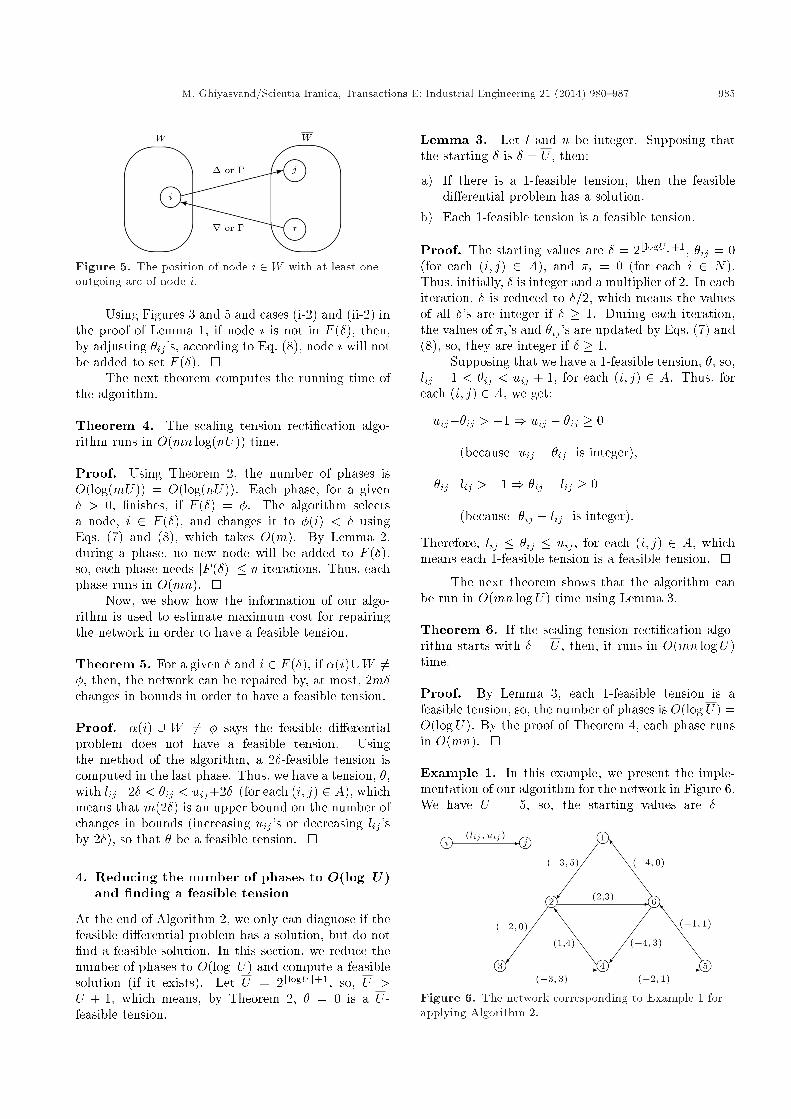
Example 1. In this example, we present the imple-mentation of our algorithm for the network in Figure 6.We have U = 5, so, the starting values are � =

Figure 6. The network corresponding to Example 1 forapplying Algorithm 2.


Figure 7. The initial values for �(i)'s and �ij 's inExample 1.

2blog5c + 1 = 8, and �i = 0 for each i 2 N (i.e.�ij = 0, for each (i; j) 2 A). The starting �(i)'s areshown in Figure 7: �(1) = 0, �(2) = 2, �(3) = 0,�(4) = 1, and �(5) = �(6) = �1. Hence, we haveF (8) = fi 2 N j 8 � �(i) < 16g = � and F (4) =fi 2 N j 4 � �(i) < 8g = �, so, we let � = 2 andget F (2) = fi 2 N j 2 � �(i) < 4g = f2g. Forthe outgoing arc (2; 6), we have �26 = 0 < l26 = 2,so �(2) = 6 and a labeling procedure (2) should bedone, so, we �rst label node 2. For the outgoing arc(2; 3), we have �23 = 0 = u23, which means (2; 3) 2 r,so, we label node 3. For the incoming arc (4; 2), wehave �42 = 0 < l42 = 1, which means (4; 2) 2 �,so, we label node 4. Other nodes can not be labeled.We have W = f2; 3; 4g, and W = f1; 5; 6g, so, �(2)is not in W . Hence, by Eqs. (7) and (8), we get�2 = �3 = �4 = 0� 2 = �2, �i = 0 (for other i 2 N),�26 = 0 + 2 = 2, �45 = 0 + 2 = 2, �12 = 0 � 2 = �2,�64 = 0� 2 = �2 and �ij = 0 for other (i; j) 2 A. Theupdated values of �(i)'s are �(1) = �(2) = �(3) = 0,�(4) = 1 and �(5) = �(6) = �1.

Now, we have F (2) = fi 2 N j 2 � �(i) < 4g = �,so we let � = 1, and get F (1) = fi 2 N j 1 � �(i) <2g = f4; 5g. By selecting node 4, updated values of �i'sare �2 = �3 = �2, �4 = �3, �5 = �1 and �i = 0 (forother i 2 N). Updated values �ij 's are �42 = �56 = 1,�34 = �1, �64 = �3; �26 = 2; �45 = 2, �12 = �2 and�ij = 0, for other (i; j) 2 A. The updated values of�(i)'s are �(1) = �(2) = �(3) = �(4) = �(6) = 0 and�(5) = 1.

Thus, F (1) = fi 2 N j 1 � �(i) < 2g = f5g.For the incoming arc (4; 5) of node 5, we have �45 =2 > u45 = 1, so, 4 2 �(5) and the labeling procedure(5) should be done, which gives W = f5; 6; 2; 4; 3g, and�(5)\W 6= �. Therefore, the problem does not have asolution. Note, in Cycle C : 5� 6� 2� 4� 5, we haved+(C) = (1 + 1)� (2 + 1) = �1 < 0.

Now, the maximum cost is estimated for repairingthis network in order to have a feasible tension. Wehave F (2) = ;, but F (1) 6= ;. Thus, by Theorem 5,an estimation of the maximum cost of repair is 2�m =2(1)(9) = 18. Of course, we have a lower estimation asfollows:

�42 = 1 = l42; �56 = 1 = u56;

l34 = �3 < �34 = �1 < u34 = 3;

l64 = �4 < �64 = �3 < u64 = 3; �26 = 2 = l26;

�45 = 2 > u45 = 1;

l12 = �3 < �12 = �2 < u12 = 5;

�61 = 0 = u61; and �23 = 0 = u23:

Thus we only need to change the upper bound arc (4; 5)by 1 unit (i.e. u45 should be increased to 2) in order torepair the network.

Acknowledgements

I would like to thank two anonymous referees for theirvaluable suggestions.

References

1. Berge, C. and Ghouila-Houri, A., Programming,Games and Transportation Networks, Wiley, New York(1962).

2. Ghouila-Houri, A. \Flows and tension in a graph"[Flots et tension dans un graph], Ph.D Thesis,Gauthier-Villars, Paris (1964).

3. Pla, J.M. \An out-of-kilter algorithm for solving mini-mum cost potential problems", Mathematical Program-ming, 1, pp. 275-290 (1971)

4. Hadjiat, M. \Penelope's graph: a hard minimum costtension instanc", Theoretical Computer Science, 194,pp. 207-218 (1998).

5. Hamacher, H.W. \Min cost tension", Journal of In-formation & Optimization Sciences, 6(3). pp. 285-304(1985).

6. Rockafeller, R.T., Network Flows and MonotropicOptimization, John Wiley and Sons (1984).

7. Hadjiat, M. and Maurras, J.F. \A strongly polynomialalgorithm for the minimum cost tension problem",Discrete Mathematics, 165/166, pp. 377-394 (1997).

8. Ghiyasvand, M. \An O(m(m+nlogn)log(nC))-time al-gorithm to solve the minimum cost tension problem",Theoretical Computer Science, 448, pp. 47-55 (2012).

9. Ghiyasvand, M. \A polynomial-time implementationof Pla's method to solve the MCT problem", Advancesin Computational Mathematics and Its Applications,1(2), pp. 104-109 (2012).

10. Ahuja, R.K., Hochbaum, D.S. and Orlin, J.B. \Solvingthe convex cost integer dual network ow problem",Management Science, 49, pp. 950-964 (2003).

11. Bachelet, B. and Duhamel, C. \Aggregation approachfor the minimum binary cost tension problem", Euro-pean Journal of Operations Research, 197, pp. 837-841(2009).


12. Bachele, B. and Mahey, P. \Minimum convex-costtension problems on series-parallel graphs", RAIROOperation Research, 37(4), pp. 221-234 (2003).

13. Bachele, B. and Mahey, P. \Minimum convex pircewiselinear cost tension problem on quasi-k series-parallelgraphs", 4OR: Quarterly Journal of European Opera-tions Research Societies, 2(4), pp. 275-291 (2004).

14. Guler, C. \Inverse tension problems and monotropicoptimization", WIMA Report (2008).

15. Goh, C.J. and Yang, X.Q., Duality in Optimizationand Variational Inequalities, Taylor and Francis, Lon-don (2002).

16. Gabow, H.N. \Scaling algorithms for network prob-lems", Journal of Computer and System Science, 31,pp. 148-168 (1985).

17. Ahuja, R.K. Magnanti, T.L. and Orlin, J.B., Net-work Flows: Theory, Algorithms, and Applications,Prentice-Hall, Englewood Cli�s, NJ (1993).

18. Minty, G.J. \On the axiomatic foundations of the theo-ries of directed linear graphs", Electrical Networks andProgramming, Journal of Mathematics and Mechanics,15, pp. 485-520 (1966).

19. Hadjiat, M. and Maurras, J.F. \Duality between ow and tension", Actes des Troisiemes Journees duGroupe MODE, Berst, France (1995).

20. Maurras, J.F. \The maximum cost tension problem",Proc. Conf., European chapter on combinatorial opti-mization (ECCO VII), Italy (1994).

Biography

Mehdi Ghiyasvand was born in Hamedan, Iran,in 1975. He obtained his MS and PhD degrees inOperations Research from Tehran University, Iran andspent a post-doctoral term at MIT University, USA. Heis now Associate Professor at Bu-Ali Sina University,Hamedan, Iran.

scaling implementation of a tension recti cation algorithm...

Documents