Metrel: Petrel Plug-in for Modeling Uncertainty inMetric Space

Kwangwon Park and Jef Caers

Stanford Center for Reservoir ForecastingDepartment of Energy Resource Engineering

Stanford University

Abstract

Modeling uncertainty for reservoir performance prediction is still a challengingand outstanding problem due to geological complexity of reservoir and CPU demand-ing flow simulations. Metric space modeling techniques deal with multiple modelsefficiently and effectively by constructing a metric space where the location of anymodel is determined exclusively by the mutual differences in responses as definedby a ”distance”. Once we know the distance between any two (geological) modelrealizations, any such model (whether a structure or property field) can be repre-sented into a metric space, which is non-dimensional but can be represented throughprojection into low-dimensional (typically 2D-5D) space through multi-dimensionalscaling. Metric space modeling techniques enable model generation (pre-image prob-lem), model selection (kernel k-means clustering), sensitivity analysis and uncertaintyassessment. We implemented core technologies (multi-dimensional scaling and ker-nel k-means clustering) for metric space modeling in the Ocean framework, whichis an application development framework that allows to develop applications tightlyintegrated with the Petrel product family. This paper aims to provide the descrip-tion and user’s guide for developed Petrel plug-in, named Metrel. Additionally, wedemonstrate the effectiveness of Metrel to modeling flow uncertainty in a 3D field-scale reservoir..

1 Introduction

Developing a plan to maximize oil production requires constructing reservoir models con-strained to all available data. Reservoir modeling is, however, still a vexed question be-cause of various sources and types of data that need to be integrated as well as the possiblyexisting uncertainty due to lack of data to fully constrain the reservoir model.

From today’s oil fields, many types of data are being obtained. One of the most im-portant data is provided by geologists. Geologists produce a geological interpretation

1

of the reservoir from outcrop or other inspections, resulting in e.g. guesses of channeldimensions, their stacking patterns or where the turbulent flow in the ocean dominateddeposition. Additionally, direct observation from a few wells is available as a form ofwell log, core, or well test data. On the other hand, indirect observation from geophys-ical survey (esp. seismic survey), often termed ”soft” data, provides a lower-resolutionconstraint. Additionally, production history (bottom hole pressure, oil or water rate) isrecorded during the production. Matching the reservoir to the production history is verydifficult due to the severe nonlinearity between the reservoir model and the history. Mod-eling a reservoir requires integration of all available data from varying scales and sources.

In particular at the appraisal stage, where reservoir production data are few and wherecritical decision need to be made, uncertainty about reservoir volume and prediction per-formance is still considerable and critical to the decision making process. Such uncertaintyis captured and represented by generating several alternative reservoir models by vary-ing key geological, geophysical and reservoir engineering parameters. Hence, a powerfultool for managing multiple reservoir models is required. In order to assess the uncer-tainty using multiple reservoir models, Monte Carlo simulation or experimental design iswidely used. However, Monte Carlo simulation demands a number of flow simulations,which is not feasible practically. Additionally, the experimental design is not applicableto spatial (geological) variables which are often categorical and critical to flow (Caers andScheidt, 2010).

Metric space modeling means that processes accompanied by modeling a reservoirare reformulated and performed in metric space, where the location of any model is de-termined exclusively by the mutual differences in responses as defined by a ”distance”.First step of all metric space modeling techniques is to define a distance to construct a met-ric space for the initial set of multiple models; Secondly the metric space is represented byits projection to the low-dimensional space by means of multi-dimensional scaling (MDS).MDS generates a map of points with maintaining the distance between any two points.MDS makes it possible to analyze the ensemble of multiple models by simple visual in-spection as well as through many statistical analysis techniques. From the constructedmetric space, a series of operations for reservoir modeling is available: generating addi-tional models (Caers, 2008; Scheidt et al., 2008), selecting a few representative models byscreening and clustering models (Scheidt and Caers, 2009a, 2010), sensitivity analysis anduncertainty assessment for models (Scheidt and Caers, 2008, 2009b), updating models forconstraining to nonlinear time-series data (Caers and Park, 2008; Park et al., 2008), and soforth (for a detailed summary, refer to Caers et al. (2010)). While a reservoir model is of-ten represented by millions of parameters (properties at each gridblock), in metric space,a reservoir model is represented by the distance between other models that is correlatedwith the output of application, which is simple and of critical interest. Also, as long asa distance between any two models is defined, metric space modeling technologies canbe applied to any combination of models, such as models of several different structuralgeometry or models of different geological scenarios.

2

Ocean is an application development framework that allows to develop applicationstightly integrated with the Petrel product family ((Schlumberger, 2008)). Under the Win-dows.NET environment, Ocean allows developing user-friendly plugins which can beexecuted in the Petrel using all the Petrel functions and database. Petrel is a reservoirmodeling software which makes it possible to generate multiple reservoir models (multi-ple structures, multiple properties, etc.) given almost all types of geological, geophysical,petrophysical data, and so on. In addition, Petrel has many strong analysis functions for3D visualization, reservoir flow simulation, uncertainty assessment, and so forth.

In this study, we have developed a Petrel plug-in (Metrel) where core technologies formetric space modeling are implemented based on the Ocean framework. First, Metrel al-lows defining any type of distance from the Petrel database. Second, Metrel constructs ametric space and map all the initial set of models into low-dimensional space by means ofMDS. The results are stored in the Petrel database and each model can be viewed and ana-lyzed in 3D display window as a point. Third, Metrel performs kernel k-means clustering(KKM) to divide the set of models into several groups for further analyses. Finally, basedon the results from MDS and clustering, sensitivity analysis and uncertainty assessmentare available. In Section 2, theories for metric space modeling are briefly described. Inchapters Sections 3 to 5, we explain how the plug-in works and how and where to useMetrel, followed by summarizing remarks in Section 6.

With Metrel, users can choose a few representative model realizations and determinethe uncertainty in future prediction (eg. P10, P50, and P90) with the reduced numberof model realizations. Additionally, users can analyze the sensitivity of any type of pa-rameters whether continuous (channel width or length) or categorical (type of structuralmodel, multiple geological scenarios). Finally, users can analyze multiple model realiza-tions very easily by means of simple visual inspection.

2 Metric space modeling

Let xi be a set of parameters that represents a model, which can often be a vector of theproperty values assigned to each gridblock or to the model itself or the combination ofboth. If the number of parameters defining a model is N and the number of models L,then a set (or ensemble) of models is represented by the matrix X (Equation 1). NoteN >> L.

X =(

x1 x2 · · · xi · · · xL)ᵀ ∈ RL×N (1)

Let gi be a set of parameters that represents an output of a model xi in which we areinterested (gi = g(xi)). For example, gi is the oil production rate calculated by reservoirsimulation of i-th model realization (g(xi)). Then the distance is defined such that the dis-tance between any two models are reasonably correlated with the difference in the outputs

3

of the two models (Equation 2). We can define any type of function for the distance calcu-lation as long as Equation 2 holds. Note the function d(xi, xj) should be computationallyeasy and fast while the evaluation of function g(xi) often costs large time and efforts.

dij = d(xi, xj) correlates with√

(gi − gj)ᵀ(gi − gj) (2)

In most cases, the size of gi is much smaller than that of xi. In other words, xi usu-ally exists in very high-dimensional (105D to 107D) space and gi in low-dimensional (1to 100) space; if we construct a metric space representing the models exclusively by thedistance, the arrangement of models in metric space is much simpler than that in the high-dimensional model space. The fact that what we are actually interested in is not the modelitself but the output from the model shows another merit of this application-tailored dis-tance, since we are focusing on the output as well as rendering the problem simple. Thisis the reason why we can represent the constructed metric space as a projection to low-dimensional (2D to 5D) space through multi-dimensional scaling.

Multi-dimensional scaling (MDS)

MDS is a process that maps the models from metric space into a low-dimensional Carte-sian space (MDS space) such that the Euclidean distance between the mapped points inMDS space is as close as possible to the application-tailored distance of Equation 2 (Equa-tion 3).

X 7→ Xm s.t. d(xi, xj) ∼=√

(xi,m − xj,m)ᵀ(xi,m − xj,m) (3)

where, the subscript mds means the point mapped by MDS. MDS is simply done by eigen-value decomposition and retaining ”reasonable” number of eigenvalues as in Equations 4to 6. ”Reasonable” means ”large enough to capture the variation of models in metricspace” and can be determined by the correlation coefficient between the distance in met-ric space and the distance in MDS space. Equation 4 represents the process of centeringthe distance matrix.

B = HAH (4)

where, H represents the centering matrix:

H = I− 1L

11ᵀ ∈ RL×L

with I of the identity matrix and 1 of a column vector of L ones (1 = [11 · · · 1]ᵀ ∈ RL×1).The element of matrix A is calculated by

aij = −12

d2ij

4

.Next, the eigenvalue decomposition of B is

B = VBΛBVᵀB (5)

where, VB denotes the collection of eigenvectors of B and ΛB the diagonal matrix of eigen-values of B. If we retain the M largest eigenvalues and the corresponding eigenvectorsto construct a small eigenvalue matrix ΛB,M and eigenvector matrix VB,M, Xm is finallyobtained by

Xm = VB,MΛ1/2B,M (6)

Kernel k-means clustering

Clustering is a useful function for selecting a few representative models, screening outincompatible models, sensitivity analysis, uncertainty assessment, and so on. In Metrelclustering is used for model selections and sensitivity analysis on geological/engineeringparameters.

Since models in metric space are mapped into a low-dimensional space using MDS,k-means clustering converges easily. More importantly, kernel techniques for clustering,which arrange the models in MDS space linearly in kernel feature space, makes the clus-tering more reliable and effective.

K-means clustering is an iterative algorithm for finding the locations of cluster cen-troids so as to minimize the sum of distances between the models and their nearest cen-troids (Equations 7). Once the locations of centroids are determined, the models nearestto each centroid are clustered into a group and assigned its cluster index (Equations 8).

Copt = argminC

L

∑i=1

minj‖cj − xi,m‖ with j = 1, 2, · · · , Nc (7)

ui = argminj‖cj,opt − xi,m‖ (8)

where, C represents the collection of cluster centroids of size M × Nc, Nc the number ofclusters predefined, and ui the cluster index for the i-th model xi. The subscript opt meansthe optimized cluster centroids.

KKM means k-means clustering in kernel feature space. First, we define a map fromMDS space to kernel space (Equations 9). In metric space modeling, a Gaussian radial-basis kernel function (k) is often selected since we have already defined a distance andradial-basis kernel function is a function of distance only (Equation 10). Then a Euclideandistance between two features in kernel space is represented by Equations 11. As seenin Equation 11, the distance in kernel space is calculated from the kernel function, whichmeans Φ does not have to be explicitly stated (the kernel trick).

5

Xm 7→ Φ s.t. k(xi,m, xj,m) = φᵀi φj (9)

k(xi,m, xj,m) = exp

(−‖xi,m − xj,m‖2

2σ2

)(10)

‖φi −φj‖2 = φᵀi φi − 2φᵀ

i φj + φᵀj φj

= 2− 2k(xi,m, xj,m) (11)

Therefore, the equations for KKM are obtained by slightly modifying Equations 7and 8 (Equations 12 and 13).

Copt = argmaxC

L

∑i=1

maxj

k(cj, xi,m) with j = 1, 2, · · · , Nc (12)

ui = argmaxj

k(cj,opt, xi,m) (13)

3 How Metrel works

In a Petrel database, three types of tabs exist: Input, Models, and Results. Input containsvarious input parameters, such as well information, fluid petrophysical properties, etc.Models contains various models that we generate from the input data. Lastly, Resultscontains simulation or analysis results, such as flow simulation results or sensitivity anal-ysis results.

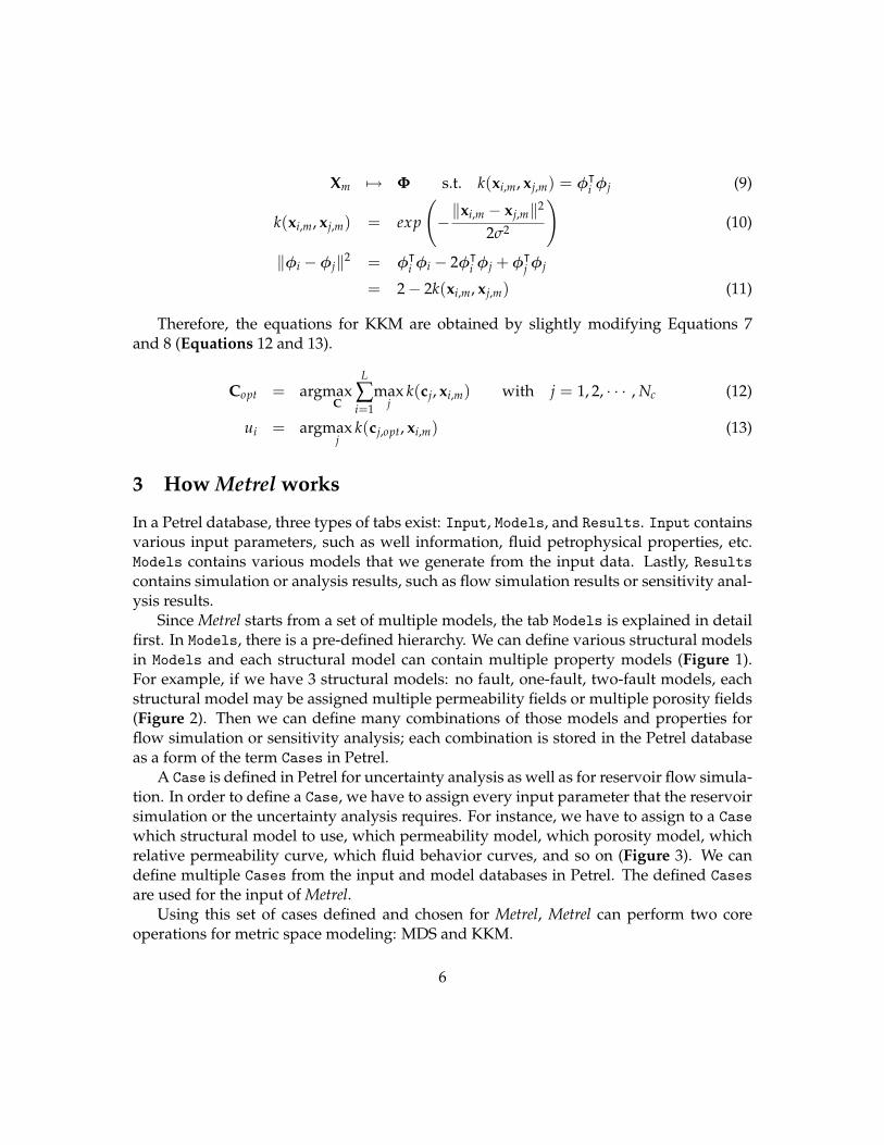
Since Metrel starts from a set of multiple models, the tab Models is explained in detailfirst. In Models, there is a pre-defined hierarchy. We can define various structural modelsin Models and each structural model can contain multiple property models (Figure 1).For example, if we have 3 structural models: no fault, one-fault, two-fault models, eachstructural model may be assigned multiple permeability fields or multiple porosity fields(Figure 2). Then we can define many combinations of those models and properties forflow simulation or sensitivity analysis; each combination is stored in the Petrel databaseas a form of the term Cases in Petrel.

A Case is defined in Petrel for uncertainty analysis as well as for reservoir flow simula-tion. In order to define a Case, we have to assign every input parameter that the reservoirsimulation or the uncertainty analysis requires. For instance, we have to assign to a Casewhich structural model to use, which permeability model, which porosity model, whichrelative permeability curve, which fluid behavior curves, and so on (Figure 3). We candefine multiple Cases from the input and model databases in Petrel. The defined Casesare used for the input of Metrel.

Using this set of cases defined and chosen for Metrel, Metrel can perform two coreoperations for metric space modeling: MDS and KKM.

6

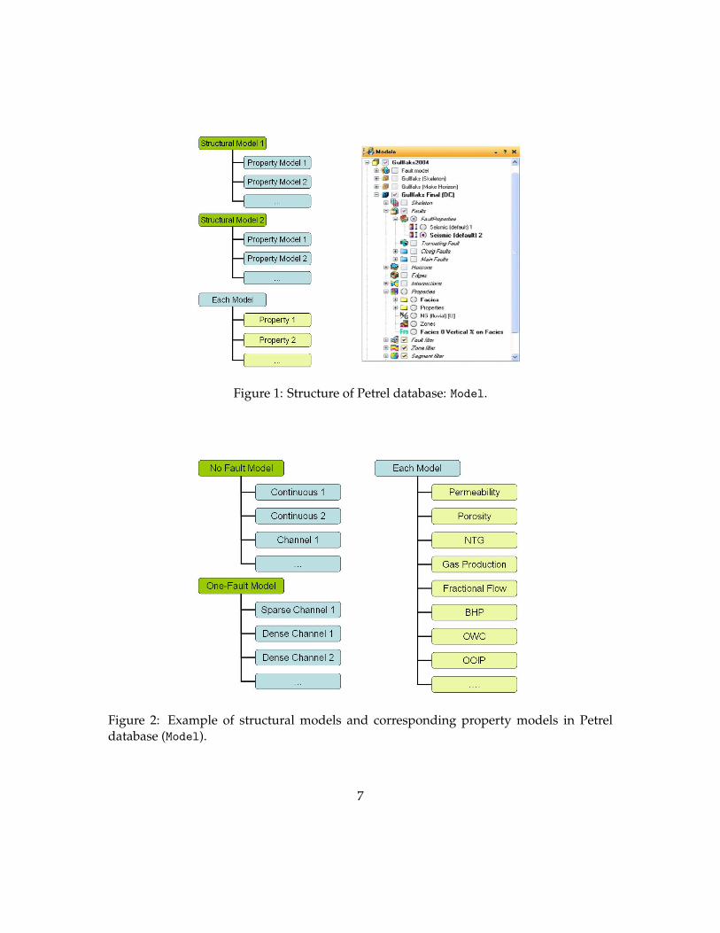
Figure 1: Structure of Petrel database: Model.

Figure 2: Example of structural models and corresponding property models in Petreldatabase (Model).

7

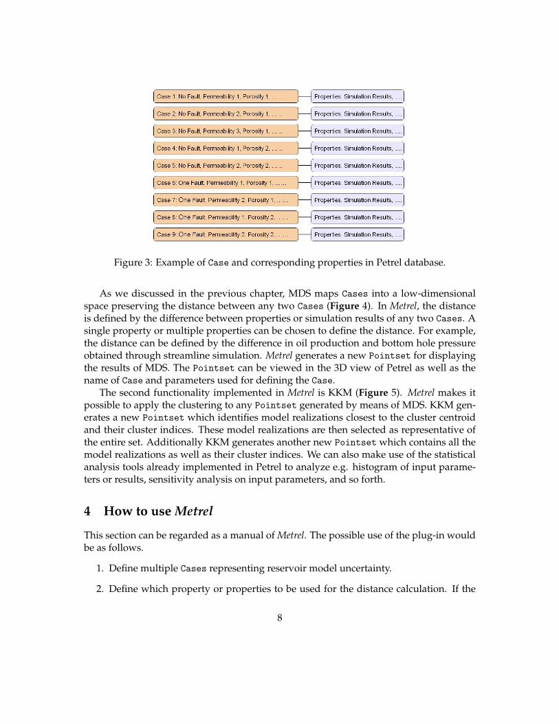
Figure 3: Example of Case and corresponding properties in Petrel database.

As we discussed in the previous chapter, MDS maps Cases into a low-dimensionalspace preserving the distance between any two Cases (Figure 4). In Metrel, the distanceis defined by the difference between properties or simulation results of any two Cases. Asingle property or multiple properties can be chosen to define the distance. For example,the distance can be defined by the difference in oil production and bottom hole pressureobtained through streamline simulation. Metrel generates a new Pointset for displayingthe results of MDS. The Pointset can be viewed in the 3D view of Petrel as well as thename of Case and parameters used for defining the Case.

The second functionality implemented in Metrel is KKM (Figure 5). Metrel makes itpossible to apply the clustering to any Pointset generated by means of MDS. KKM gen-erates a new Pointset which identifies model realizations closest to the cluster centroidand their cluster indices. These model realizations are then selected as representative ofthe entire set. Additionally KKM generates another new Pointset which contains all themodel realizations as well as their cluster indices. We can also make use of the statisticalanalysis tools already implemented in Petrel to analyze e.g. histogram of input parame-ters or results, sensitivity analysis on input parameters, and so forth.

4 How to use Metrel

This section can be regarded as a manual of Metrel. The possible use of the plug-in wouldbe as follows.

1. Define multiple Cases representing reservoir model uncertainty.

2. Define which property or properties to be used for the distance calculation. If the

8

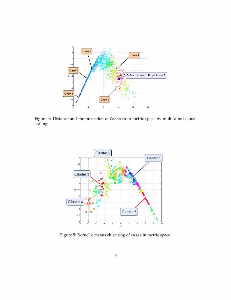
Figure 4: Distance and the projection of Cases from metric space by multi-dimensionalscaling.

Figure 5: Kernel k-means clustering of Cases in metric space.

9

distance is defined by the difference in flow responses, we advocate using streamlinesimulation (Frontsim in Petrel) for all the Cases defined. Evaluation of the distanceneeds to be relatively efficient.

3. Run Metrel. The Metrel user-interface would display all the Cases and the Propertieswhich are shared by all the Cases.

4. Choose which Cases to be used for MDS and which Properties to be used for dis-tance calculation (Figure 6). The Map multiple models into the metric spacebutton executes MDS and a new Pointset is generated in the Input tab of the Petreldatabase. The new Pointset represents the location of each Case in MDS space andits name (Figure 7). Also any other properties can be added into the Pointset byusing the function Edit From Spreadsheet in the Pointset.

5. Go to the next tab: Clustering. Choose which metric space to be used for theclustering (Figure 6). The other parameters (dimension of metric space and ker-nel bandwidth) are determined automatically by clicking the buttons located on theright-hand side of the input boxes (for details about how to choose it automatically,see Scheidt and Caers (2009b)). The only parameter that needs to be determined bythe user is the number of clusters. Then the clustered results in the new Pointset isadded in the Input tab. The new Pointset additionally contains the cluster indicesand centroids information (Figure 8).

5 How to use Metrel: an example application

We apply Metrel to the Brugge field synthetic data set, which is generated for testing opti-mization and history matching methods (Peters et al., 2009). The objective is to assess theuncertainty in 10-year prediction of oil production and analyze the sensitivity of genera-tion methods of permerbility and porosity on the oil production. Figure 9 shows reservoirgeometry and wells which are introduced into the Petrel database:

• Geometry: A high-resolution model of 20 million gridblocks and a flow-simulationmodel of 60,048 gridblocks are provided.

• Wells: There are 20 production wells and 10 injection wells.

• Property: 104 property models of varying net-to-gross ratio (NTG), permeability(PERMX, PERMY, PERMZ), and porosity (PORO) are given. Table 1 displays howthe porosity and permeability models are generated. 78 models are generated basedon facies (FIgure 10) and the remaining 26 models are generated without faciesinformation(Figure 11). Among 78 models generated with facies information, 39porosity models are generated by the multiple-point geostatistical simulation (MPS)

10

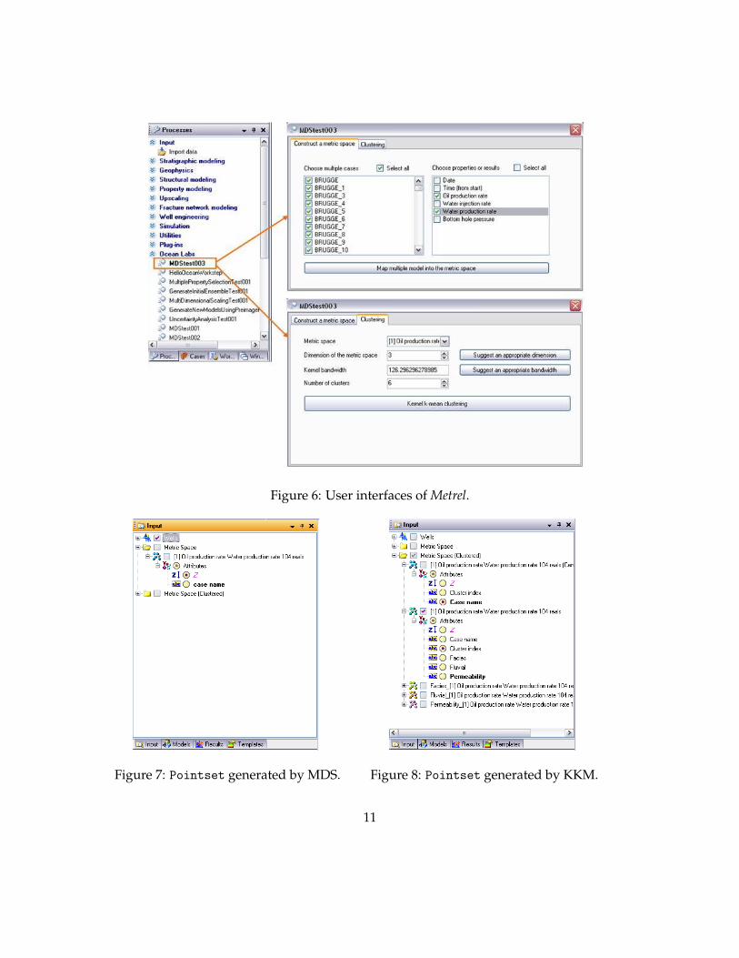
Figure 6: User interfaces of Metrel.

Figure 7: Pointset generated by MDS. Figure 8: Pointset generated by KKM.

11

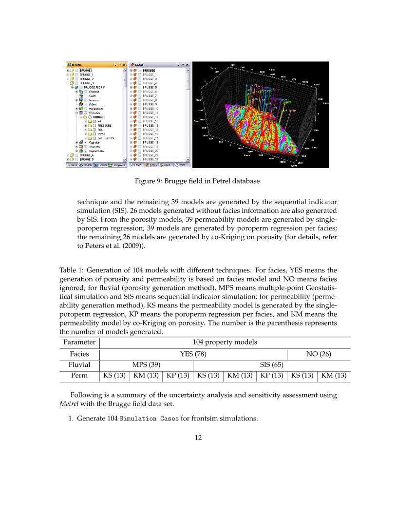
Figure 9: Brugge field in Petrel database.

technique and the remaining 39 models are generated by the sequential indicatorsimulation (SIS). 26 models generated without facies information are also generatedby SIS. From the porosity models, 39 permeability models are generated by single-poroperm regression; 39 models are generated by poroperm regression per facies;the remaining 26 models are generated by co-Kriging on porosity (for details, referto Peters et al. (2009)).

Table 1: Generation of 104 models with different techniques. For facies, YES means thegeneration of porosity and permeability is based on facies model and NO means faciesignored; for fluvial (porosity generation method), MPS means multiple-point Geostatis-tical simulation and SIS means sequential indicator simulation; for permeability (perme-ability generation method), KS means the permeability model is generated by the single-poroperm regression, KP means the poroperm regression per facies, and KM means thepermeability model by co-Kriging on porosity. The number is the parenthesis representsthe number of models generated.

Parameter 104 property models

Facies YES (78) NO (26)Fluvial MPS (39) SIS (65)Perm KS (13) KM (13) KP (13) KS (13) KM (13) KP (13) KS (13) KM (13)

Following is a summary of the uncertainty analysis and sensitivity assessment usingMetrel with the Brugge field data set.

1. Generate 104 Simulation Cases for frontsim simulations.

12

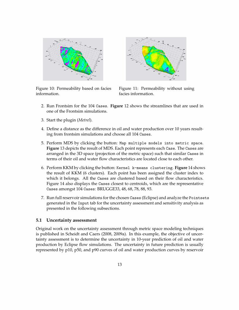
Figure 10: Permeability based on faciesinformation.

Figure 11: Permeability without usingfacies information.

2. Run Frontsim for the 104 Cases. Figure 12 shows the streamlines that are used inone of the Frontsim simulations.

3. Start the plugin (Metrel).

4. Define a distance as the difference in oil and water production over 10 years result-ing from frontsim simulations and choose all 104 Cases.

5. Perform MDS by clicking the button: Map multiple models into metric space.Figure 13 depicts the result of MDS. Each point represents each Case. The Cases arearranged in the 3D space (projection of the metric space) such that similar Cases interms of their oil and water flow characteristics are located close to each other.

6. Perform KKM by clicking the button: Kernel k-means clustering. Figure 14 showsthe result of KKM (6 clusters). Each point has been assigned the cluster index towhich it belongs. All the Cases are clustered based on their flow characteristics.Figure 14 also displays the Cases closest to centroids, which are the representativeCases amongst 104 Cases: BRUGGE33, 48, 68, 78, 88, 93.

7. Run full reservoir simulations for the chosen Cases (Eclipse) and analyze the Pointsetsgenerated in the Input tab for the uncertainty assessment and sensitivity analysis aspresented in the following subsections.

5.1 Uncertainty assessment

Original work on the uncertainty assessment through metric space modeling techniquesis published in Scheidt and Caers (2008, 2009a). In this example, the objective of uncer-tainty assessment is to determine the uncertainty in 10-year prediction of oil and waterproduction by Eclipse flow simulations. The uncertainty in future prediction is usuallyrepresented by p10, p50, and p90 curves of oil and water production curves by reservoir

13

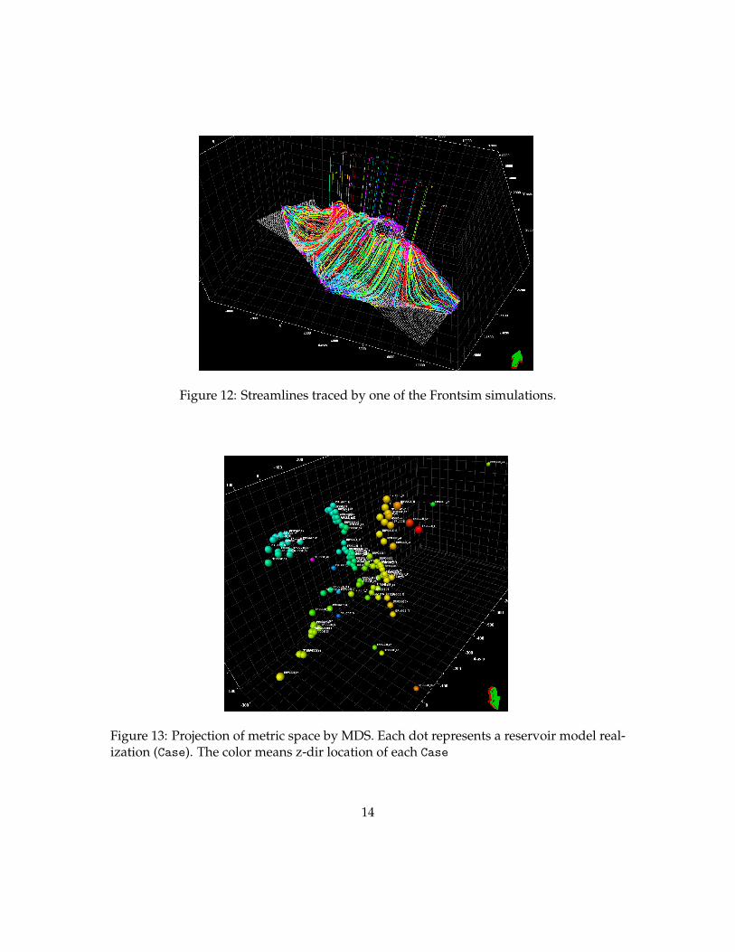
Figure 12: Streamlines traced by one of the Frontsim simulations.

Figure 13: Projection of metric space by MDS. Each dot represents a reservoir model real-ization (Case). The color means z-dir location of each Case

14

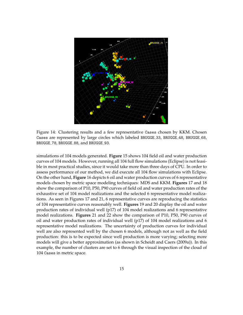
Figure 14: Clustering results and a few representative Cases chosen by KKM. ChosenCases are represented by large circles which labeled BRUGGE 33, BRUGGE 48, BRUGGE 68,BRUGGE 78, BRUGGE 88, and BRUGGE 93.

simulations of 104 models generated. Figure 15 shows 104 field oil and water productioncurves of 104 models. However, running all 104 full flow simulations (Eclipse) is not feasi-ble in most practical studies, since it would take more than three days of CPU. In order toassess performance of our method, we did execute all 104 flow simulations with Eclipse.On the other hand, Figure 16 depicts 6 oil and water production curves of 6 representativemodels chosen by metric space modeling techniques: MDS and KKM. Figures 17 and 18show the comparison of P10, P50, P90 curves of field oil and water production rates of theexhaustive set of 104 model realizations and the selected 6 representative model realiza-tions. As seen in Figures 17 and 21, 6 representative curves are reproducing the statisticsof 104 representative curves reasonably well. Figures 19 and 20 display the oil and waterproduction rates of individual well (p17) of 104 model realizations and 6 representativemodel realizations. Figures 21 and 22 show the comparison of P10, P50, P90 curves ofoil and water production rates of individual well (p17) of 104 model realizations and 6representative model realizations. The uncertainty of production curves for individualwell are also represented well by the chosen 6 models, although not as well as the fieldproduction: this is to be expected since well production is more varying; selecting moremodels will give a better approximation (as shown in Scheidt and Caers (2009a)). In thisexample, the number of clusters are set to 6 through the visual inspection of the cloud of104 Cases in metric space.

15

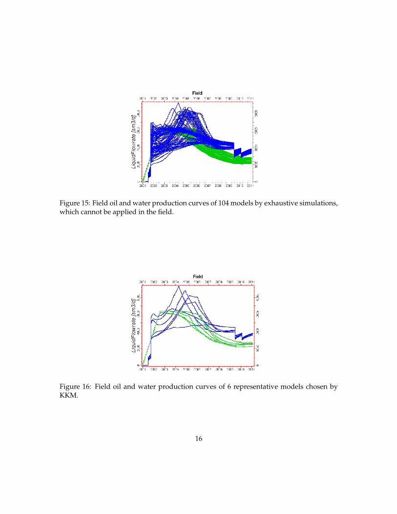
Figure 15: Field oil and water production curves of 104 models by exhaustive simulations,which cannot be applied in the field.

Figure 16: Field oil and water production curves of 6 representative models chosen byKKM.

16

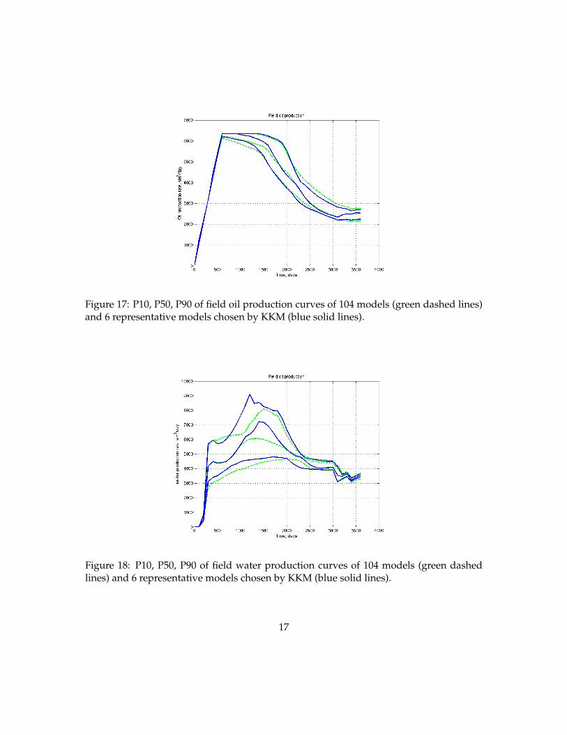
Figure 17: P10, P50, P90 of field oil production curves of 104 models (green dashed lines)and 6 representative models chosen by KKM (blue solid lines).

Figure 18: P10, P50, P90 of field water production curves of 104 models (green dashedlines) and 6 representative models chosen by KKM (blue solid lines).

17

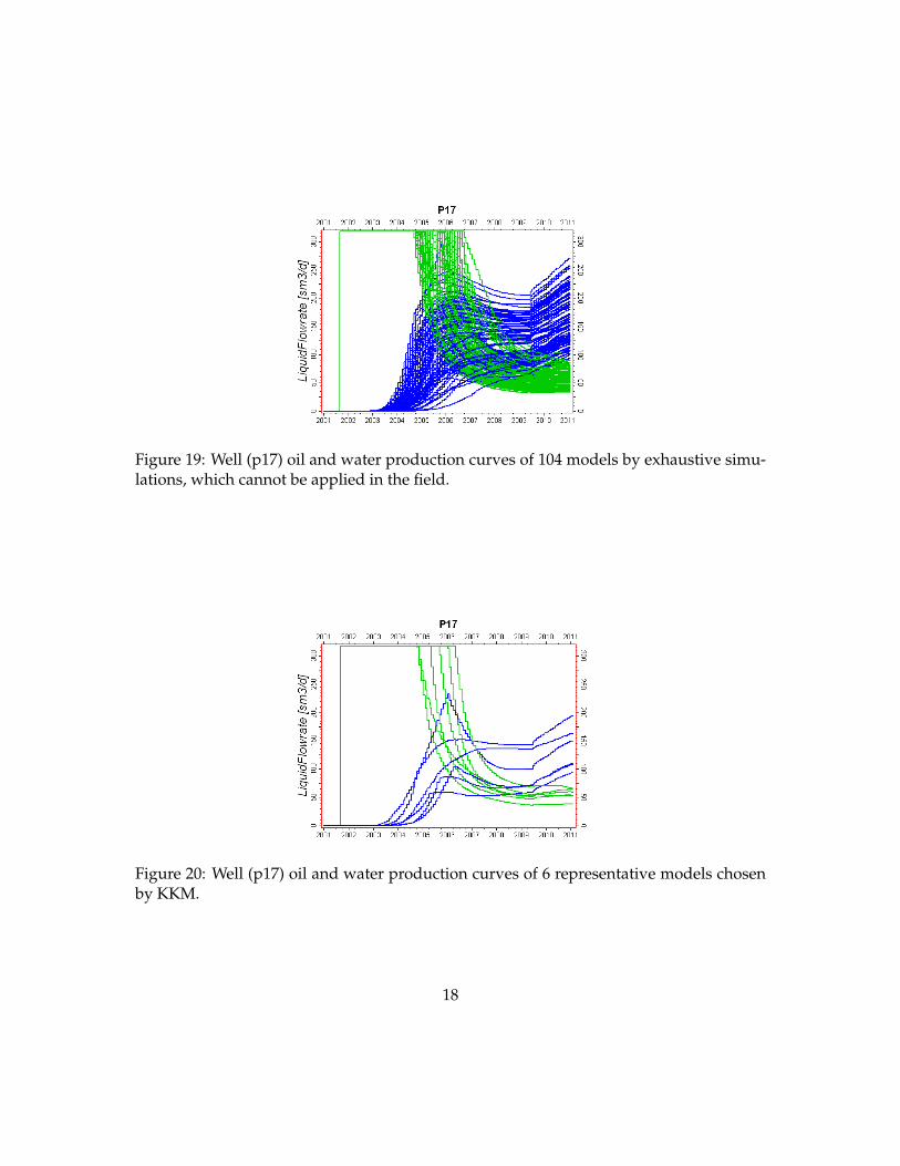
Figure 19: Well (p17) oil and water production curves of 104 models by exhaustive simu-lations, which cannot be applied in the field.

Figure 20: Well (p17) oil and water production curves of 6 representative models chosenby KKM.

18

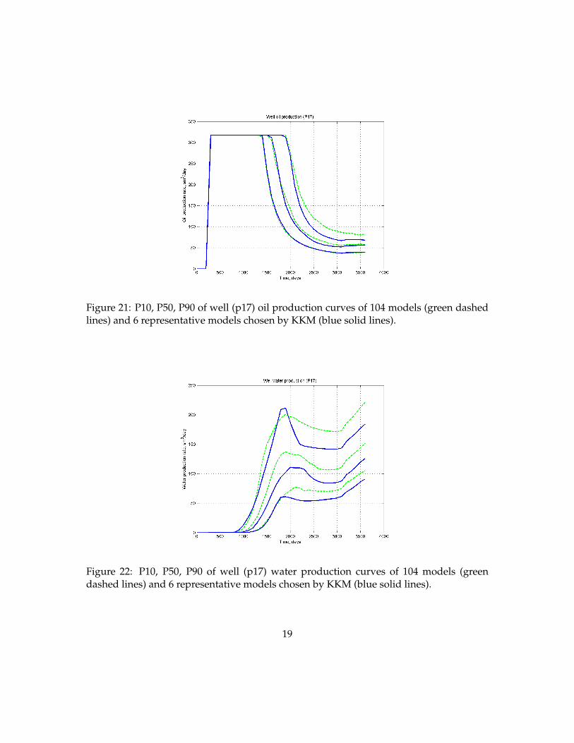
Figure 21: P10, P50, P90 of well (p17) oil production curves of 104 models (green dashedlines) and 6 representative models chosen by KKM (blue solid lines).

Figure 22: P10, P50, P90 of well (p17) water production curves of 104 models (greendashed lines) and 6 representative models chosen by KKM (blue solid lines).

19

5.2 Sensitivity analysis

In this example, the 104 porosity and permeability models are generated by different tech-niques: facies-based or not, porosity by MPS or SIS, and permeability by single poropermregression or poroperm regression per facies or coKriging on porosity. Hence, a possibleobjective of sensitivity analysis would be to determine which parameter is the most criti-cal for future prediction of oil and water production or how influential the parameter is.This can also be achieved from the results of Metrel run.

In Petrel, those generation methods (YES or NO, MPS or SIS, and KS or KM or KP; seeTable 1) can be added as a new Attribute to the Pointset generated by MDS or KKM.Figure 23 shows how those input parameters are introduced into the Petrel database andcan be edited by the users. (Note that the current version of Ocean (version 2009.2) doesnot allow the users to access those input parameters from Cases but the new version ofOcean (version 2010.1, however not available at the time of plugin development) wouldallow the access. So with Ocean 2010.1 the input parameters can also be automaticallydisplayed.) Figure 24 shows the input parameters of the 6 representative Cases selectedby KKM of Metrel. Then, the user can display the metric space with the input parametersas in Figures 25 to 27.

Figure 25 shows the Cases on the left-hand side as indicated by NO, which means thoseare generated without considering facies information, while the Cases on the right-handside are all YES. Likewise, the porosity generation method (MPS or SIS) divides the Caseshorizontally. The Cases located at the upper side of map are generated by SIS, and theCases in the lower side of map by MPS (Figure 26). More importantly, the Cases are clus-tered by themselves based on the permeability generation technique (KS or KM or KP)(Figure 27). Therefore, facies information and porosity generation method have a sensi-tivity to the future prediction oil and water production to some extent but the permeabilitygeneration technique is more important in prediction of future flow performance.

6 Summary

We have developed a petrel plug-in (Metrel) using Ocean development framework. Me-trel enables core technologies of metric space modeling (MDS and KKM) in Petrel. Metrelallows us to analyze multiple models in 2D or 3D view of Petrel or other Petrel analysisfunctions. Metrel can choose a few representative models amongst a set of multiple mod-els, which would help the efficient further analyses, such as calculating P10, P50, and P90of prediction from reservoir flow simulations. Metrel helps to analyze the sensitivity ofthe input parameters or methods to the results interested. An example run of Metrel withthe Brugge field-scale data set exhibits that 6 representative models chosen by Metrel and6 full flow simulations are enough to assess the uncertainty and analyze the sensitivity.

20

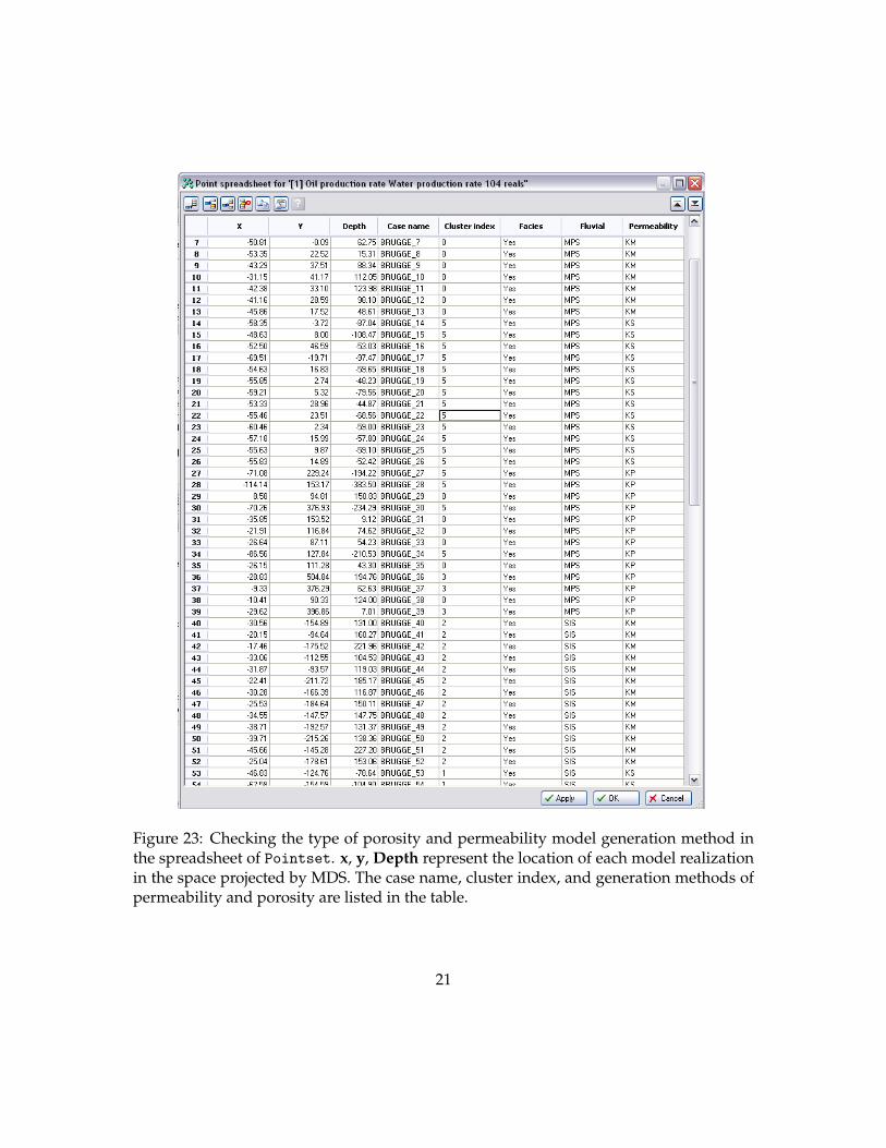
Figure 23: Checking the type of porosity and permeability model generation method inthe spreadsheet of Pointset. x, y, Depth represent the location of each model realizationin the space projected by MDS. The case name, cluster index, and generation methods ofpermeability and porosity are listed in the table.

21

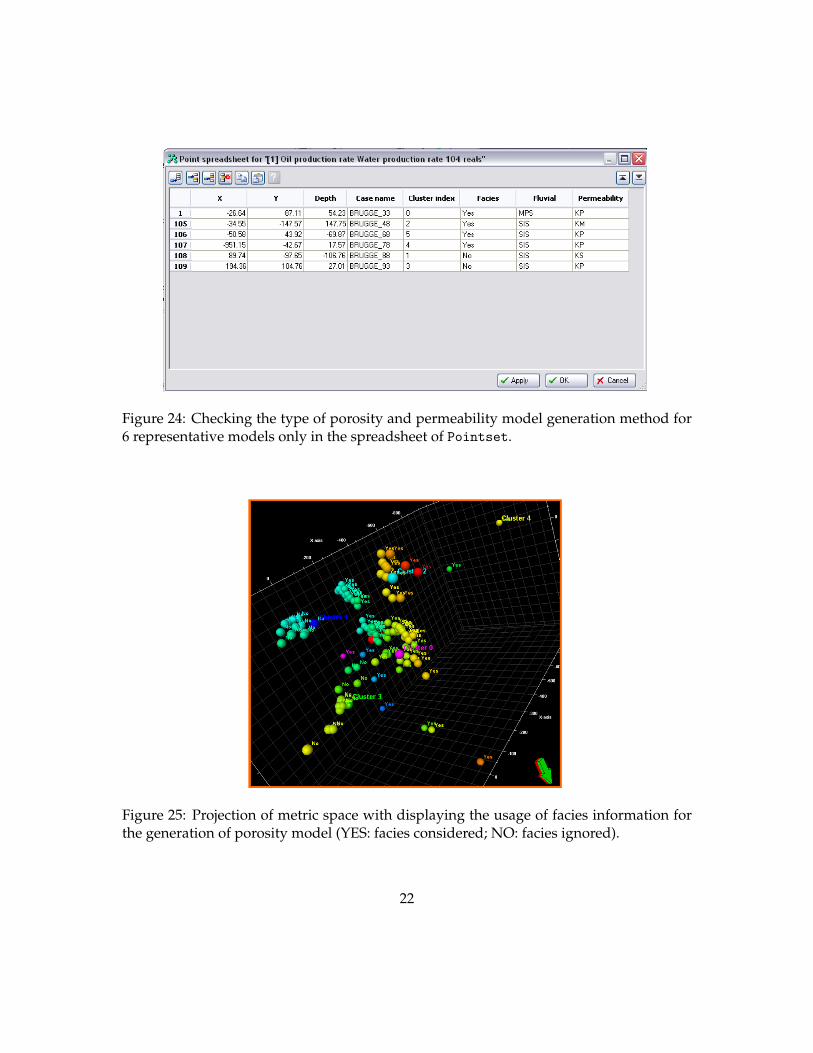
Figure 24: Checking the type of porosity and permeability model generation method for6 representative models only in the spreadsheet of Pointset.

Figure 25: Projection of metric space with displaying the usage of facies information forthe generation of porosity model (YES: facies considered; NO: facies ignored).

22

Figure 26: Projection of metric space with displaying the type of simulation method togenerate porosity model (MPS: multiple-point geostatistical method; SIS: sequential indi-cator simulation).

Figure 27: Projection of metric space with displaying the type of method to generate per-meability model (KS: single poroperm regression; KP: poroperm regression per facies;KM: coKriging on porosity).

23

References

Caers, J., Dec. 2008. Distance-based random field models and their applications. In: Pro-ceedings of 8th International Geostatistical Congress. Santiago, Chile.

Caers, J., Park, K., Sep. 2008. A distance-based representation of reservoir uncertainty: themetric enkf. In: Proceedings of 11th European Conference on the Mathematics of OilRecovery. Bergen, Norway.

Caers, J., Scheidt, C., 2010. Joint integration of engineering and geological uncertainty forreservoir performance prediction using a distance-based approach. In AAPG Memoiron Modeling Geological Uncertainty in press.

Caers, J., Scheidt, C., Park, K., 2010. Modeling Uncertainty of Complex Earth Systems inMetric Space. Handbook of Geomathematics in press.

Park, K., Scheidt, C., Caers, J., 2008. Ensemble Kalman Filtering in Distance-based KernelSpace. In: Proceedings of EnKF Workshop 2008. Voss, Norway.

Peters, E., Arts, R., Brouwer, G., Geel, C., 2009. Results of the Brugge Benchmark Study forFlooding Optimisation and History Matching. SPE Reservoir Simulation Symposium12 (1), 105–119.

Scheidt, C., Caers, J., Sep. 2008. Joint quantification of uncertainty on spatial and non-spatial reservoir parameters Comparison between the Joint Modeling Method and Dis-tance Kernel Method. In: Proceedings of 11th European Conference on the Mathematicsof Oil Recovery. Bergen, Norway.

Scheidt, C., Caers, J., 2009a. A new method for uncertainty quantification using distancesand kernel methods. Application to a deepwater turbidite reservoir. SPE Journal 14 (4),680–692, spe118740-PA.

Scheidt, C., Caers, J., 2009b. Representing Spatial Uncertainty Using Distances and Ker-nels. Mathemathcal Geosciences 41 (4), 397–419.

Scheidt, C., Caers, J., 2010. Bootstrap confidence intervals for reservoir model selectiontechniques. Computational Geosciences 14 (2), 369–382.

Scheidt, C., Park, K., Caers, J., Dec. 2008. Defining a Random Function from a GivenSet of Model Realizations. In: Proceedings of 8th International Geostatistical Congress.Santiago, Chile.

Schlumberger, 2008. Ocean: Developer’s Guide (Volume 1: Core and Services).

24