sea ice in the caspian sea - osi saf hlosisaf.met.no/docs/report_caspian_ice.pdf · concentration...
TRANSCRIPT
Ocean & Sea Ice SAF
Associate & Visiting Scientist Activity Report
Sea Ice in the Caspian Sea
Reference: OSI_AS11_P04
Version 1.0
September 2011
Peygham Ghaffari, UiOLeif Toudal Pedersen, DMISteinar Eastwood, met.noThomas Lavergne, met.no

OSI_AS11_P04
Documentation Change Record
Version Date Author Description1.0 09-2011 P.G et al. First version
EUMETSAT OSI SAF 2 of 54 Version 1.0 – September 2011
OSI_AS11_P04
CONTENTS
1. Introduction ...................................................................................................................... 4 1.1 Objective from OSI-SAF proposal .............................................................................. 4 1.2 Study area .................................................................................................................. 4 1.3 OSI-SAF Overview ..................................................................................................... 4 1.4 Main target ................................................................................................................. 5 1.5 Ownership and copyright of data ................................................................................ 5 1.6 Acknowledgment ........................................................................................................ 5 1.7 Glossary ..................................................................................................................... 5
2. Input data and Algorithms ................................................................................................. 7 2.1 SSM/I data set ............................................................................................................ 7 2.2 AMSR-E data set ........................................................................................................ 8 2.3 Ice chart ...................................................................................................................... 8 2.4 Algorithms .................................................................................................................. 9
3. Data treatment and processing ...................................................................................... 10 3.1 Area selection ........................................................................................................... 10 3.2 Available data ........................................................................................................... 11 3.3 Selection of data ....................................................................................................... 12 3.4 Data screening ......................................................................................................... 13
4. Tie-points (SSM/I) .......................................................................................................... 20 4.1 Open water tie-points for the CS .............................................................................. 20 4.2 Ice tie-points ............................................................................................................. 21
5. Sea Ice retrieval algorithms (SSM/I) .............................................................................. 25 5.1 Bristol algorithm ........................................................................................................ 25 5.2 Comiso Bootstrap algorithm (BF) ............................................................................. 27 5.3 OSI SAF hybrid algorithm ........................................................................................ 29
6. AMSR-E dataset ............................................................................................................. 30 6.1 Data treating (AMSR-E) ............................................................................................ 30 6.2 tie-points(AMSR-E) ................................................................................................... 31 6.3 Sea ice concentration retrieval (AMSR-E) ................................................................ 32
7. Monthly tie-points ........................................................................................................... 35 8. Verification against ice charts ......................................................................................... 43
8.1 Overall description of verification .............................................................................. 43 8.2 Verification against ice chart ..................................................................................... 43
9. Concluding remarks ....................................................................................................... 51 10. Acknowledgement ........................................................................................................ 52 11. References .................................................................................................................. 53
EUMETSAT OSI SAF 3 of 54 Version 1.0 – September 2011
OSI_AS11_P04
1. Introduction
1.1 Objective from OSI-SAF proposal
The ECMWF has made a request to the OSI-SAF to extend the operational sea ice concentration product to also cover the Caspian Sea (CS) which is currently not in the OSI-SAF products grid. In this context the OSI-SAF Sea Ice Team proposed present scientific activity aimed to:
– study the sea ice concentration in the CS, validate the performance of the sea ice concentration algorithms is this region.
– Development, test and implementation of a dedicated algorithm tie-point set for the CS based on available low resolution SSM/I and high resolution AMSR-E passive microwave data as well as ice charts.
1.2 Study area
The Caspian Sea (CS) is the largest inland water body of the world that lies in among Azerbaijan, Iran, Kazakhstan, Russia and Turkmenistan (Ghaffari et al., 2010) with the surface area of 379000 km2, a drainage area of approx. 3.5 million km2 and volume of 78000 km3 (Froehlich et al., 1999). This lake is located at Northern Hemisphere between latitudes 36o and 45o covering various bathymetric levels. According to the bathymetric features and morphological characters the CS conventionally separated into northern, central and southern basins (Ghaffari and Chegini, 2010). the surface area of the three basins are roughly equal and the northern basin with maximum depth about 20 m is a very thin extension of the central basin (Peeters et al., 2000).Stable ice cover forms every year mostly in the northern and partly in the central CS and stays for several months. This seasonal ice cover could negatively affect navigation conditions and economic activity in the coastal areas and on the shelf, such as Russian and Kazakh oil rigs operating in the Northern Caspian . the CS is located on the extreme southern threshold of sea ice cover development in the Northern Hemisphere. Ice cover over the CS is subjected to significant temporal and spatial variability, influenced by climate conditions, wind fields and water currents, as well as sea morphology (Kouraev et al., 2004). Using in situ observations and airborne survey, ice cover in the CS have been studies regularly in the first half of the last century but stopped in the 1984-1985.(Terziev et al., 1992). Thus it is very important to utilizing satellite data in order to driving continuous times series of ice cover parameters such as ice concentration and duration of ice season. Obviously ice properties information are useful for various purposes like as navigation, protection of industrial objects (particularly oil industry in the northern CS), environmental conditions and climate variability as well as for forcing and verification of general circulation models ( Rayner et al., 2002) .
1.3 OSI-SAF Overview
The Ocean and Sea Ice Satellite Application Facilities, OSI-SAF, is a part of EUMETSAT distributed ground segment for production of a range of air-sea interface products that started in 1997. those near real times OSI-SAF deliverables are: sea ice characteristics, Sea Surface Temperature (SST), radiative flux and wind, surface solar Irradiance (SSI), and Downward Long-wave Irradiance (DLI). The sea ice products are sea ice concentration, sea ice edge, sea ice type and sea ice drift and mainly produced at the OSI-SAF High Latitude
EUMETSAT OSI SAF 4 of 54 Version 1.0 – September 2011
OSI_AS11_P04
processing facilities (HL center). While the OSI-SAF project is managed by CMS, Meteo-France, the HL center operated jointly by the Norwegian Meteorological institute and Danish Meteorological Institute.
1.4 Main target
There are several approaches for estimating ice cover concentration using passive microwave satellite data (Steffen et al., 1992; Comiso, 1986; Swift and Cav-alieri, 1985). Brightness temperature (TB) data are commonly utilized in most of these algorithms. But such algorithms for instance Bristol and TUD algorithms are mainly developed for Arctic or Antarctic conditions which contain the most extensive ice coverage. The main purposes of present study is developing open water, type A and sea ice,type B tie points for the CS. The archived gridded SSM/I and AMSR-E brightness temperatures over 4 years were used in order to achieve brightness and emissivities tie points. Validation is an important part of SAF product definitions. In general available sea ice sources and references in terms of possessing an acceptable level of quality, coverage and processing are comparably few. In the case of the CS it is even more difficult to find reliable sources. One of the available references is ice charts which have proper coverage over the north CS. The OSI SAF ice concentration was compared with the gridded ice chart concentration. The available algorithms could be modified by imposing new tie points which are specified for the CS.We expect some orders of improvements in terms of distinguishing between ice and open water in the CS.
1.5 Ownership and copyright of data
The ice chart data used in the project are the property of AGIP oil.
1.6 Acknowledgment
The ice chart database used in the project was generously supplied by AGIP oil.
1.7 Glossary
ASCII American Standard Code for Information Interchange
AMSR-E Advanced Microwave Scanning Radiometer-Earth
CS The Caspian Sea
DMI Danish Meteorological Institute
DMSP Defense Meteorological Satellite Program
ECMWF European Centre for Medium range Weather Forecast
EUMETSAT European Organization for the Exploration of Meteorological Satellite
HL High Latitude
met.no Norwegian Meteorological Institute
NetCDF Network Common Data Form
OSI SAF Ocean and Sea Ice Satellite Application Facility
RSS Remote Sensing Systems
EUMETSAT OSI SAF 5 of 54 Version 1.0 – September 2011

OSI_AS11_P04
SAR Synthetic Aperture Radar
SSM/I Special Sensor Microwave/Imager
TUD Technical University of Denmark
EUMETSAT OSI SAF 6 of 54 Version 1.0 – September 2011
OSI_AS11_P04
2. Input data and Algorithms
This chapter describes the main input data that have been used for the OSI-SAF sea ice concentrations reprocessing.
2.1 SSM/I data set
The Special Sensor Microwave/Imager (SSM/I) dataset used for this reprocessing was purchased by EUMETSAT from Remote Sensing Systems (RSS). In present scientific activity the version 6 of the RSS SSM/I data sets of satellites 13, 14 and 15 were utilized. In fact the RSS SSM/I version 6 pass through a quality control and correction procedure which is documented in the RSS SSM/I User's Manual (see Wents, 1991; Wentz, 1993; Wentz, 2006). The RSS SSMI geophysical datasets collected by SSM/I and SSMIS instruments carried on-board the DMSP series of polar orbiting satellites which are provided in Table 1. The brightness temperatures (tb's) were facilitated from converting antenna temperature of SSM/I (see Eastwood et al., 2011). The SSM/I is a seven-channel, four-frequency, orthogonally polarized, passive microwave radiometric system that measures atmospheric, ocean and terrain microwave brightness temperatures at 19.35, 22.2, 37.0, and 85.5 GHz. The high frequency channels possess twice sampling rate. Some more information regarding frequency channels and their characteristic are given in Table 2.
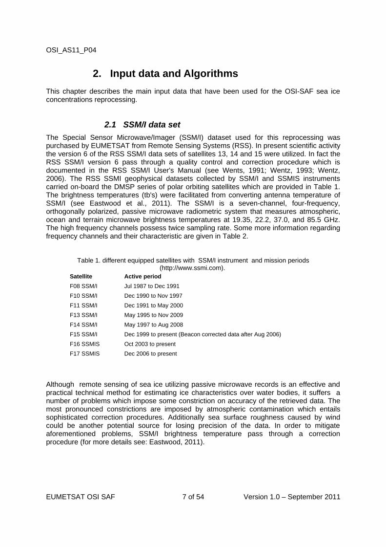
Table 1. different equipped satellites with SSM/I instrument and mission periods (http://www.ssmi.com).
Satellite Active period
F08 SSM/I Jul 1987 to Dec 1991
F10 SSM/I Dec 1990 to Nov 1997
F11 SSM/I Dec 1991 to May 2000
F13 SSM/I May 1995 to Nov 2009
F14 SSM/I May 1997 to Aug 2008
F15 SSM/I Dec 1999 to present (Beacon corrected data after Aug 2006)
F16 SSMIS Oct 2003 to present
F17 SSMIS Dec 2006 to present
Although remote sensing of sea ice utilizing passive microwave records is an effective and practical technical method for estimating ice characteristics over water bodies, it suffers a number of problems which impose some constriction on accuracy of the retrieved data. The most pronounced constrictions are imposed by atmospheric contamination which entails sophisticated correction procedures. Additionally sea surface roughness caused by wind could be another potential source for losing precision of the data. In order to mitigate aforementioned problems, SSM/I brightness temperature pass through a correction procedure (for more details see: Eastwood, 2011).
EUMETSAT OSI SAF 7 of 54 Version 1.0 – September 2011
OSI_AS11_P04
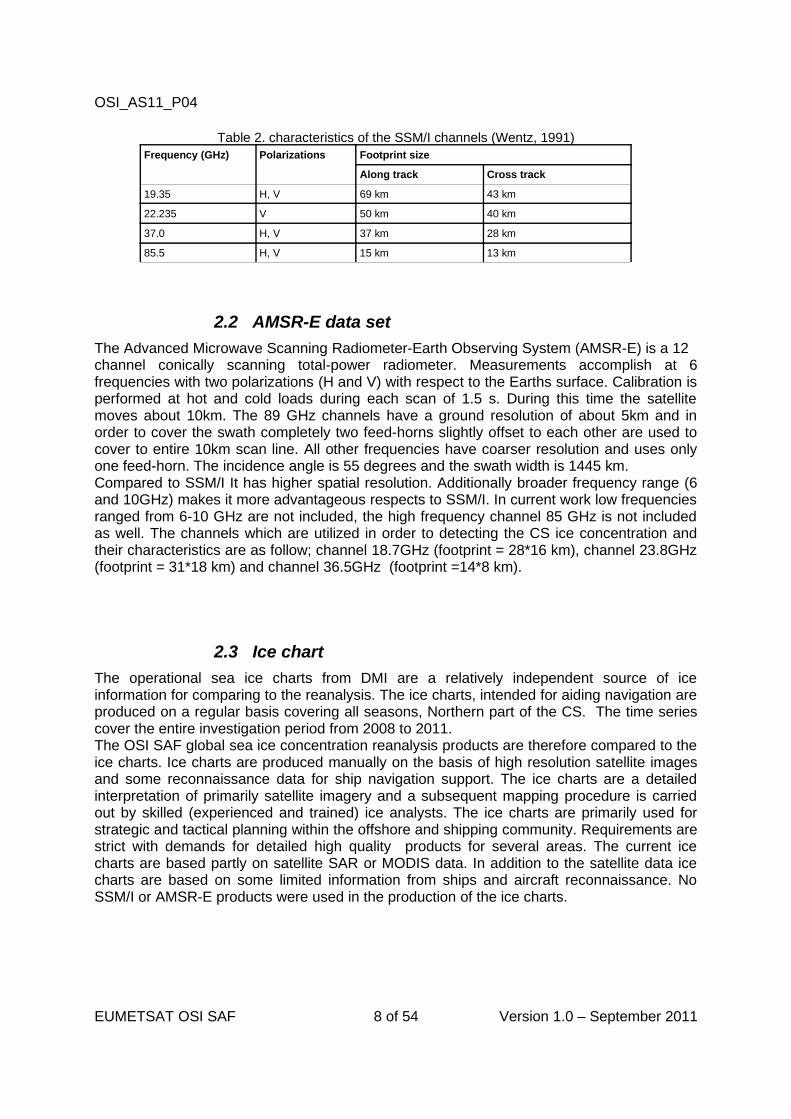
Table 2. characteristics of the SSM/I channels (Wentz, 1991)Frequency (GHz) Polarizations Footprint size
Along track Cross track
19.35 H, V 69 km 43 km
22.235 V 50 km 40 km
37.0 H, V 37 km 28 km
85.5 H, V 15 km 13 km
2.2 AMSR-E data set
The Advanced Microwave Scanning Radiometer-Earth Observing System (AMSR-E) is a 12 channel conically scanning total-power radiometer. Measurements accomplish at 6 frequencies with two polarizations (H and V) with respect to the Earths surface. Calibration is performed at hot and cold loads during each scan of 1.5 s. During this time the satellite moves about 10km. The 89 GHz channels have a ground resolution of about 5km and in order to cover the swath completely two feed-horns slightly offset to each other are used to cover to entire 10km scan line. All other frequencies have coarser resolution and uses only one feed-horn. The incidence angle is 55 degrees and the swath width is 1445 km.Compared to SSM/I It has higher spatial resolution. Additionally broader frequency range (6 and 10GHz) makes it more advantageous respects to SSM/I. In current work low frequencies ranged from 6-10 GHz are not included, the high frequency channel 85 GHz is not included as well. The channels which are utilized in order to detecting the CS ice concentration and their characteristics are as follow; channel 18.7GHz (footprint = 28*16 km), channel 23.8GHz (footprint = 31*18 km) and channel 36.5GHz (footprint =14*8 km).
2.3 Ice chart
The operational sea ice charts from DMI are a relatively independent source of ice information for comparing to the reanalysis. The ice charts, intended for aiding navigation are produced on a regular basis covering all seasons, Northern part of the CS. The time series cover the entire investigation period from 2008 to 2011.The OSI SAF global sea ice concentration reanalysis products are therefore compared to the ice charts. Ice charts are produced manually on the basis of high resolution satellite images and some reconnaissance data for ship navigation support. The ice charts are a detailed interpretation of primarily satellite imagery and a subsequent mapping procedure is carried out by skilled (experienced and trained) ice analysts. The ice charts are primarily used for strategic and tactical planning within the offshore and shipping community. Requirements are strict with demands for detailed high quality products for several areas. The current ice charts are based partly on satellite SAR or MODIS data. In addition to the satellite data ice charts are based on some limited information from ships and aircraft reconnaissance. No SSM/I or AMSR-E products were used in the production of the ice charts.
EUMETSAT OSI SAF 8 of 54 Version 1.0 – September 2011
OSI_AS11_P04
2.4 Algorithms
Two different algorithms aimed to facilitate ice concentration were utilized to reprocess the passive satellite microwave data record from 2008 to 2011. The Bristol algorithm (smith, 1996) and the Bootstrap algorithm in frequency mode (Comiso, 1986; Comiso et al., 1997) were the two algorithms that ice concentration in the northern part of the CS were estimated based on them. Additionally a combination of those two algorithms as a hybrid algorithm (OSI SAF algorithm) was applied to SSM/I brightness temperature data sets (for more detailed descriptions of the algorithms, criteria of selection see Eastwood et al., 2011).
EUMETSAT OSI SAF 9 of 54 Version 1.0 – September 2011
OSI_AS11_P04
3. Data treatment and processing
In this chapter we described the methods of data treatments and procedures were applied to available data in order to produce OSI SAF sea ice concentration.
3.1 Area selection
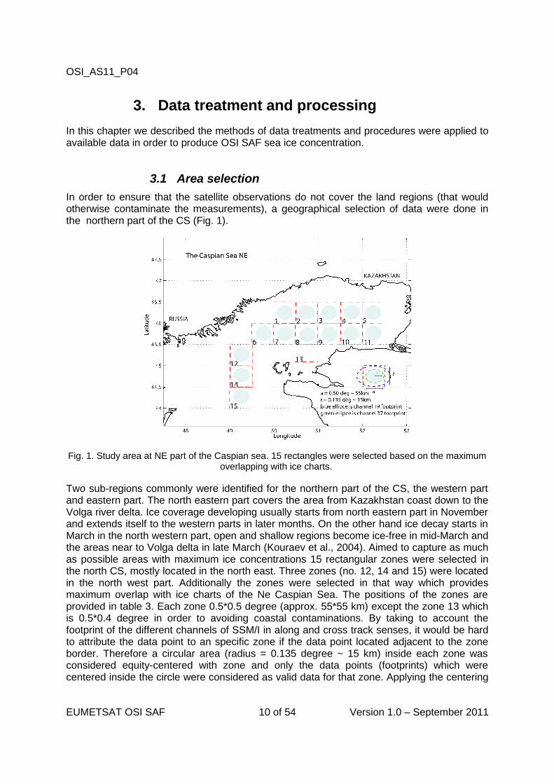
In order to ensure that the satellite observations do not cover the land regions (that would otherwise contaminate the measurements), a geographical selection of data were done in the northern part of the CS (Fig. 1).
Fig. 1. Study area at NE part of the Caspian sea. 15 rectangles were selected based on the maximum overlapping with ice charts.
Two sub-regions commonly were identified for the northern part of the CS, the western part and eastern part. The north eastern part covers the area from Kazakhstan coast down to the Volga river delta. Ice coverage developing usually starts from north eastern part in November and extends itself to the western parts in later months. On the other hand ice decay starts in March in the north western part, open and shallow regions become ice-free in mid-March and the areas near to Volga delta in late March (Kouraev et al., 2004). Aimed to capture as much as possible areas with maximum ice concentrations 15 rectangular zones were selected in the north CS, mostly located in the north east. Three zones (no. 12, 14 and 15) were located in the north west part. Additionally the zones were selected in that way which provides maximum overlap with ice charts of the Ne Caspian Sea. The positions of the zones are provided in table 3. Each zone 0.5*0.5 degree (approx. 55*55 km) except the zone 13 which is 0.5*0.4 degree in order to avoiding coastal contaminations. By taking to account the footprint of the different channels of SSM/I in along and cross track senses, it would be hard to attribute the data point to an specific zone if the data point located adjacent to the zone border. Therefore a circular area (radius = 0.135 degree ~ 15 km) inside each zone was considered equity-centered with zone and only the data points (footprints) which were centered inside the circle were considered as valid data for that zone. Applying the centering
EUMETSAT OSI SAF 10 of 54 Version 1.0 – September 2011
OSI_AS11_P04
procedure to each zone, providing higher chance for data points to be located inside the zones and the majority of the extracted data for an specific zone could be attributable to that zone.
Table 3. rectangles positions, each pair in upper row is Lon and each pair in lower row is Lat Zone no.
1 2 3 4 5 6 7 8 9 10 11 12 13 14 15
Lon 50.00
50.50
50.50
51.00
51.00
51.50
51.50
52.0
52.00
52.50
49.45
50.00
50.00
50.50
50.50
51.00
51.00
51.50
51.50
52.00
52.00
52.50
49.00
49.50
50.50
51.00
49.00
49.50
49.00
49.50
Lat 46.50
46.00
46.50
46.00
46.50
46.00
46.50
46.00
46.50
46.00
46.00
45.50
46.00
45.50
46.00
45.50
46.00
45.50
46.00
45.50
46.00
45.50
45.50
45.00
45.50
45.10
45.00
44.50
44.45
43.00
3.2 Available data
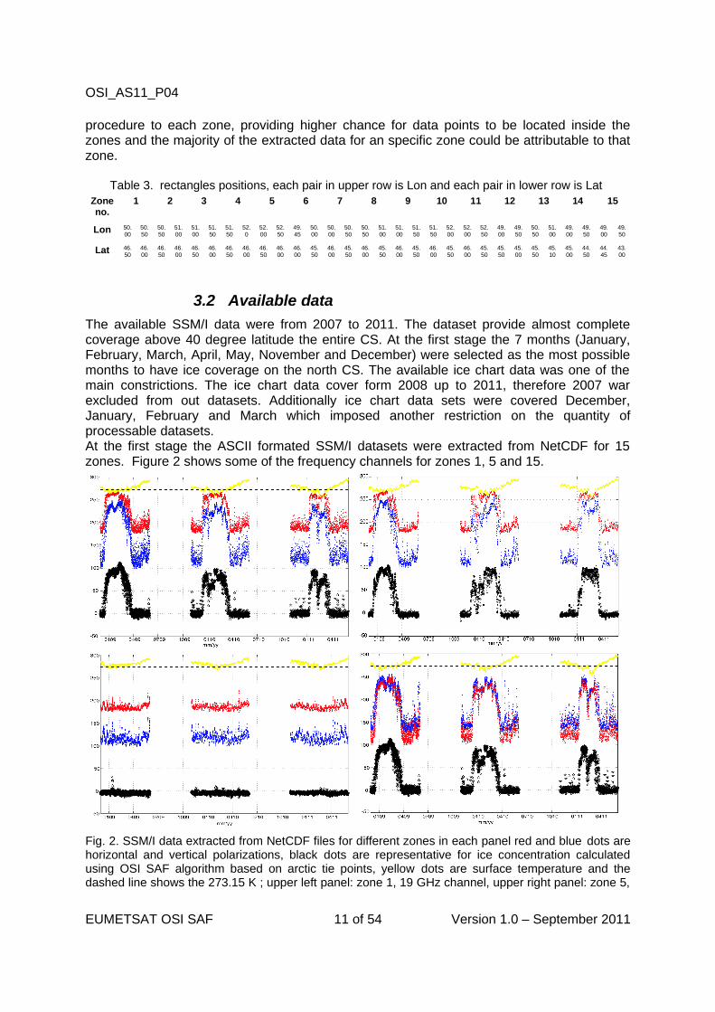
The available SSM/I data were from 2007 to 2011. The dataset provide almost complete coverage above 40 degree latitude the entire CS. At the first stage the 7 months (January, February, March, April, May, November and December) were selected as the most possible months to have ice coverage on the north CS. The available ice chart data was one of the main constrictions. The ice chart data cover form 2008 up to 2011, therefore 2007 war excluded from out datasets. Additionally ice chart data sets were covered December, January, February and March which imposed another restriction on the quantity of processable datasets. At the first stage the ASCII formated SSM/I datasets were extracted from NetCDF for 15 zones. Figure 2 shows some of the frequency channels for zones 1, 5 and 15.
Fig. 2. SSM/I data extracted from NetCDF files for different zones in each panel red and blue dots are horizontal and vertical polarizations, black dots are representative for ice concentration calculated using OSI SAF algorithm based on arctic tie points, yellow dots are surface temperature and the dashed line shows the 273.15 K ; upper left panel: zone 1, 19 GHz channel, upper right panel: zone 5,
EUMETSAT OSI SAF 11 of 54 Version 1.0 – September 2011
OSI_AS11_P04
19 GHz channel, lower left panel: zone 15, 19 GHz channel, lower right panel: zone 1, 37 GHz channel.
Based on the preliminarily graphs in Fig. 2 during some specific period e.g., January 2010 and February 2011 despite to decreasing the brightness temperature and surface temperature values, noticeable reductions in sea ice concentrations are evident. Those periods were investigated using available ice chart maps in order to getting some notion about the agreement between SSM/I and ice chart data set. According to ice chart maps it could be confirmed that sea ice concentrations followed more or less resemblance trends at those periods. Sea ice concentration data were extracted for 15 predefined zones using ice chart gridded datasets. Sea ice concentration in ice charts usually assigned by values from 0 to 10 where 0 is representative for sea ice concentration and 10 is equal to 100% ice. Additionally it is quite common that some points are assigned by 9+ which in our procedure is translated to 95% sea ice concentration. In our study area high sea ice concentration in the north east of the CS were mostly assigned by 9+ and there were just few 100% sea ice concentration areas.
3.3 Selection of data
Obviously the overlapping datasets between SSM/I and ice charts supposed to be selected at this stage. The available ice chart datasets are mostly released at some limited hours as: 02, 06, 07, 17 and 18, therefore extracting the datasets which were exactly at the same time would reduced the data points quantity extremely. In order to extract the most corresponding data points between SSM/I and ice charts datasets the following conditions were applied:
– data points located at the same rectangle– the time deference between SSM/I and ice chart datasets less than 6 hrs
The time lag between the real satellite imagery time and the mapping time in ice charts could be up to 12 hrs. The 6 hrs threshold was chosen in that way which in the worst case maximum time difference between ice charts and SSM/I datasets do not exceed 18 hrs. By applying this method the ice chart and SSM/I corresponding data sets could be considered for same day where we do not expect that much variations in ice concentration in each zone.
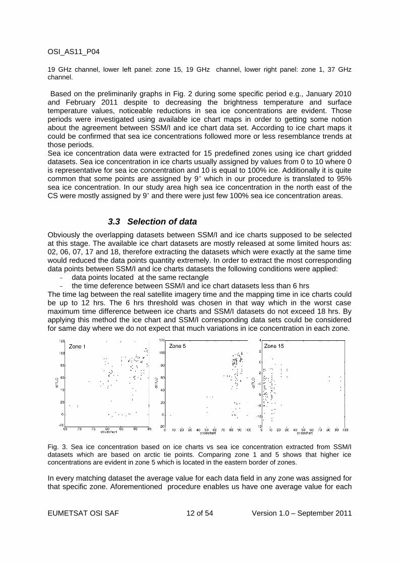
Fig. 3. Sea ice concentration based on ice charts vs sea ice concentration extracted from SSM/I datasets which are based on arctic tie points. Comparing zone 1 and 5 shows that higher ice concentrations are evident in zone 5 which is located in the eastern border of zones.
In every matching dataset the average value for each data field in any zone was assigned for that specific zone. Aforementioned procedure enables us have one average value for each
EUMETSAT OSI SAF 12 of 54 Version 1.0 – September 2011
OSI_AS11_P04
data filed in an specific time for one zone. It is worth to mention that all SSM/I data points which are located inside the 15 km radius circle were attributed to zones and other data points were discarded even if located inside the zone but not inside the circle. Figure 3 illustrates extracted concentrations from ice charts and SSM/I datasets in some zones for whole period. Zone 5 which is located in the extreme eastern border of selected zones considerably possess more high sea ice concentration values. Furthermore zone 15 at western part of the north CS shows mostly low ice concentration values. In all zones some data points demonstrate low and high ice concentration based on SSM/I and ice chart respectively. New thin ice coverage could be captured properly with ice charts production procedures. SSM/I brightness temperatures are known to be poorly sensitive to new thin ice (Kouraev et al, 2004). Therefore some areas could be assigned as high ice coverage in ice charts while based in SSM/I bright temperature those areas could be sensed as ice free. The difference in capturing the thin new ice coverage could be potential source of discrepancies in some data points.
3.4 Data screening
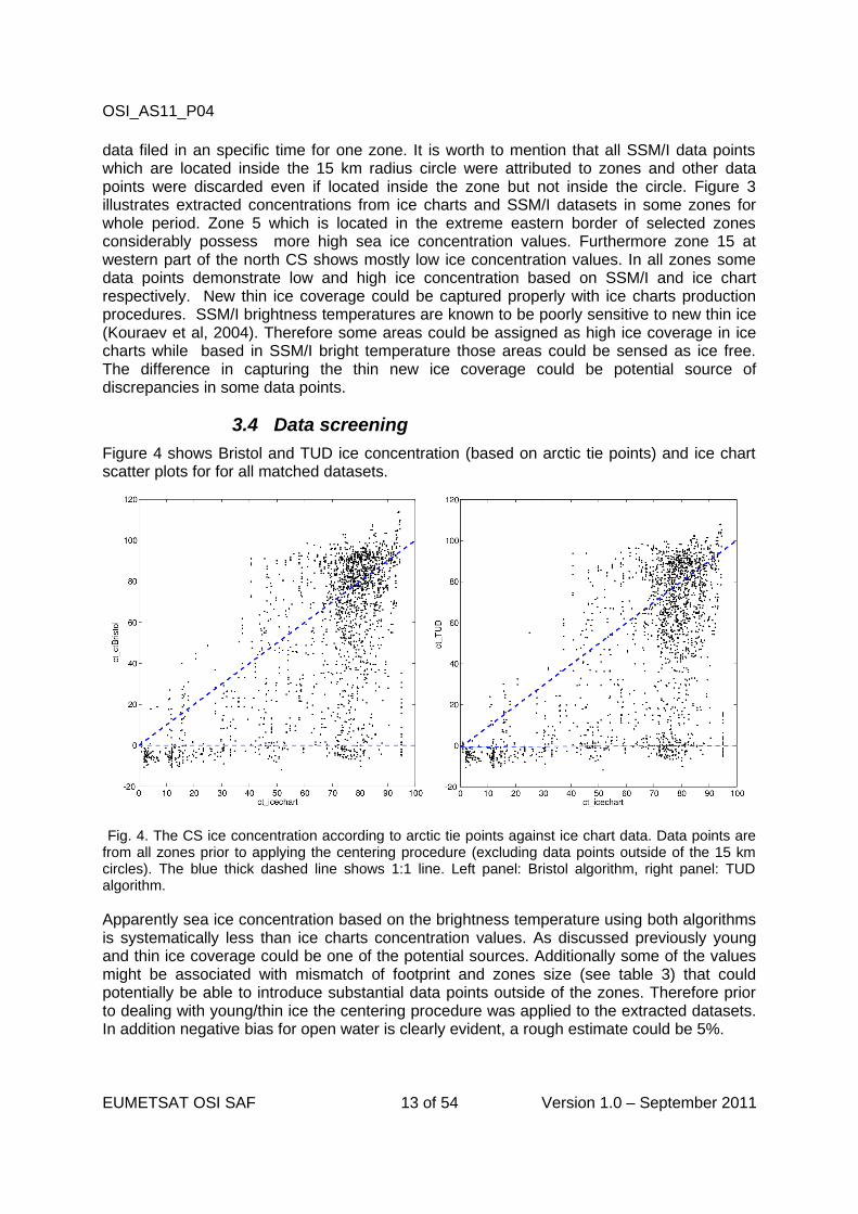
Figure 4 shows Bristol and TUD ice concentration (based on arctic tie points) and ice chart scatter plots for for all matched datasets.
Fig. 4. The CS ice concentration according to arctic tie points against ice chart data. Data points are from all zones prior to applying the centering procedure (excluding data points outside of the 15 km circles). The blue thick dashed line shows 1:1 line. Left panel: Bristol algorithm, right panel: TUD algorithm.
Apparently sea ice concentration based on the brightness temperature using both algorithms is systematically less than ice charts concentration values. As discussed previously young and thin ice coverage could be one of the potential sources. Additionally some of the values might be associated with mismatch of footprint and zones size (see table 3) that could potentially be able to introduce substantial data points outside of the zones. Therefore prior to dealing with young/thin ice the centering procedure was applied to the extracted datasets. In addition negative bias for open water is clearly evident, a rough estimate could be 5%.
EUMETSAT OSI SAF 13 of 54 Version 1.0 – September 2011
OSI_AS11_P04
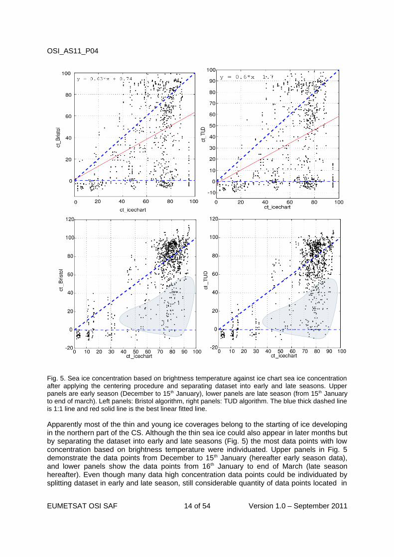
Fig. 5. Sea ice concentration based on brightness temperature against ice chart sea ice concentration after applying the centering procedure and separating dataset into early and late seasons. Upper panels are early season (December to 15th January), lower panels are late season (from 15th January to end of march). Left panels: Bristol algorithm, right panels: TUD algorithm. The blue thick dashed line is 1:1 line and red solid line is the best linear fitted line.
Apparently most of the thin and young ice coverages belong to the starting of ice developing in the northern part of the CS. Although the thin sea ice could also appear in later months but by separating the dataset into early and late seasons (Fig. 5) the most data points with low concentration based on brightness temperature were individuated. Upper panels in Fig. 5 demonstrate the data points from December to 15th January (hereafter early season data), and lower panels show the data points from 16th January to end of March (late season hereafter). Even though many data high concentration data points could be individuated by splitting dataset in early and late season, still considerable quantity of data points located in
EUMETSAT OSI SAF 14 of 54 Version 1.0 – September 2011
OSI_AS11_P04
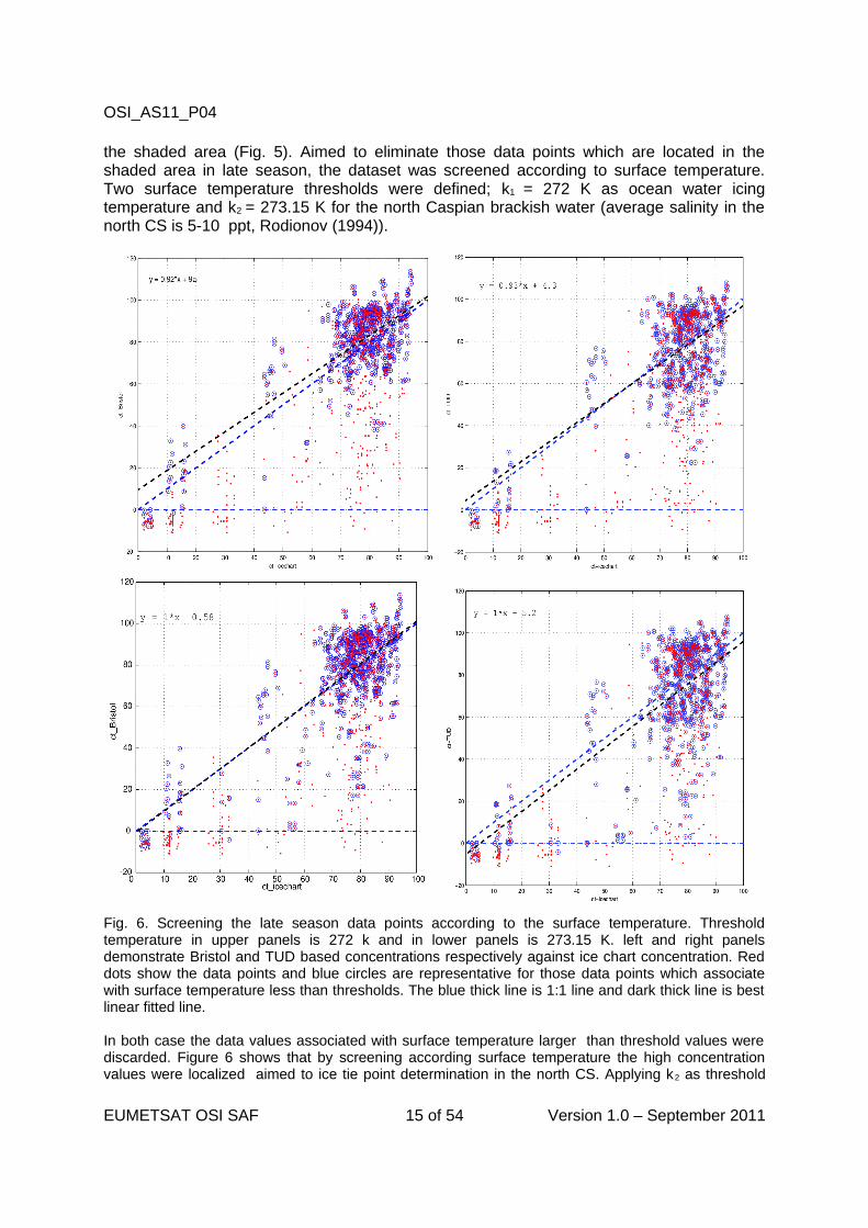
the shaded area (Fig. 5). Aimed to eliminate those data points which are located in the shaded area in late season, the dataset was screened according to surface temperature. Two surface temperature thresholds were defined; k1 = 272 K as ocean water icing temperature and k2 = 273.15 K for the north Caspian brackish water (average salinity in the north CS is 5-10 ppt, Rodionov (1994)).
Fig. 6. Screening the late season data points according to the surface temperature. Threshold temperature in upper panels is 272 k and in lower panels is 273.15 K. left and right panels demonstrate Bristol and TUD based concentrations respectively against ice chart concentration. Red dots show the data points and blue circles are representative for those data points which associate with surface temperature less than thresholds. The blue thick line is 1:1 line and dark thick line is best linear fitted line.
In both case the data values associated with surface temperature larger than threshold values were discarded. Figure 6 shows that by screening according surface temperature the high concentration values were localized aimed to ice tie point determination in the north CS. Applying k2 as threshold
EUMETSAT OSI SAF 15 of 54 Version 1.0 – September 2011
OSI_AS11_P04
provides better agreement between 1:1 line and best linear fitted line but utilizing k1 threshold consequents less data points in shaded area. Therefore the dataset with surface temperature less than k1 was considered as final dataset for tie point determination.
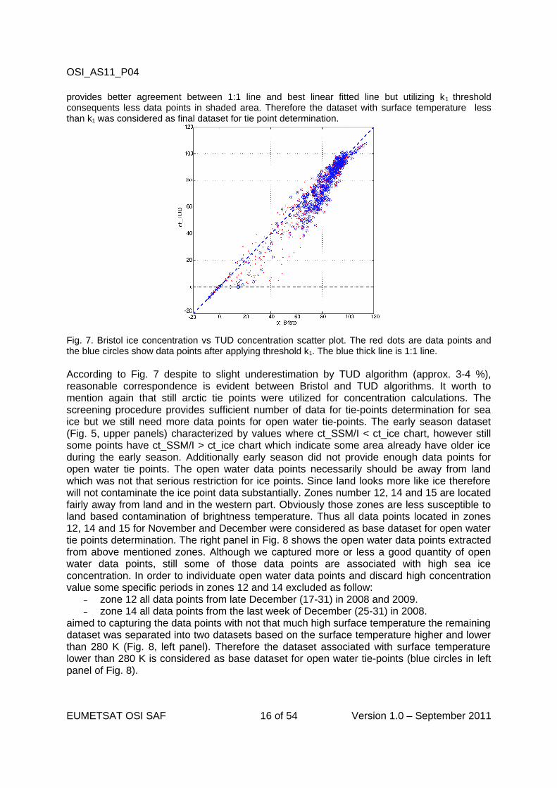
Fig. 7. Bristol ice concentration vs TUD concentration scatter plot. The red dots are data points and the blue circles show data points after applying threshold k1. The blue thick line is 1:1 line.
According to Fig. 7 despite to slight underestimation by TUD algorithm (approx. 3-4 %), reasonable correspondence is evident between Bristol and TUD algorithms. It worth to mention again that still arctic tie points were utilized for concentration calculations. The screening procedure provides sufficient number of data for tie-points determination for sea ice but we still need more data points for open water tie-points. The early season dataset (Fig. 5, upper panels) characterized by values where ct_SSM/I < ct_ice chart, however still some points have ct_SSM/I > ct_ice chart which indicate some area already have older ice during the early season. Additionally early season did not provide enough data points for open water tie points. The open water data points necessarily should be away from land which was not that serious restriction for ice points. Since land looks more like ice therefore will not contaminate the ice point data substantially. Zones number 12, 14 and 15 are located fairly away from land and in the western part. Obviously those zones are less susceptible to land based contamination of brightness temperature. Thus all data points located in zones 12, 14 and 15 for November and December were considered as base dataset for open water tie points determination. The right panel in Fig. 8 shows the open water data points extracted from above mentioned zones. Although we captured more or less a good quantity of open water data points, still some of those data points are associated with high sea ice concentration. In order to individuate open water data points and discard high concentration value some specific periods in zones 12 and 14 excluded as follow:
– zone 12 all data points from late December (17-31) in 2008 and 2009.– zone 14 all data points from the last week of December (25-31) in 2008.
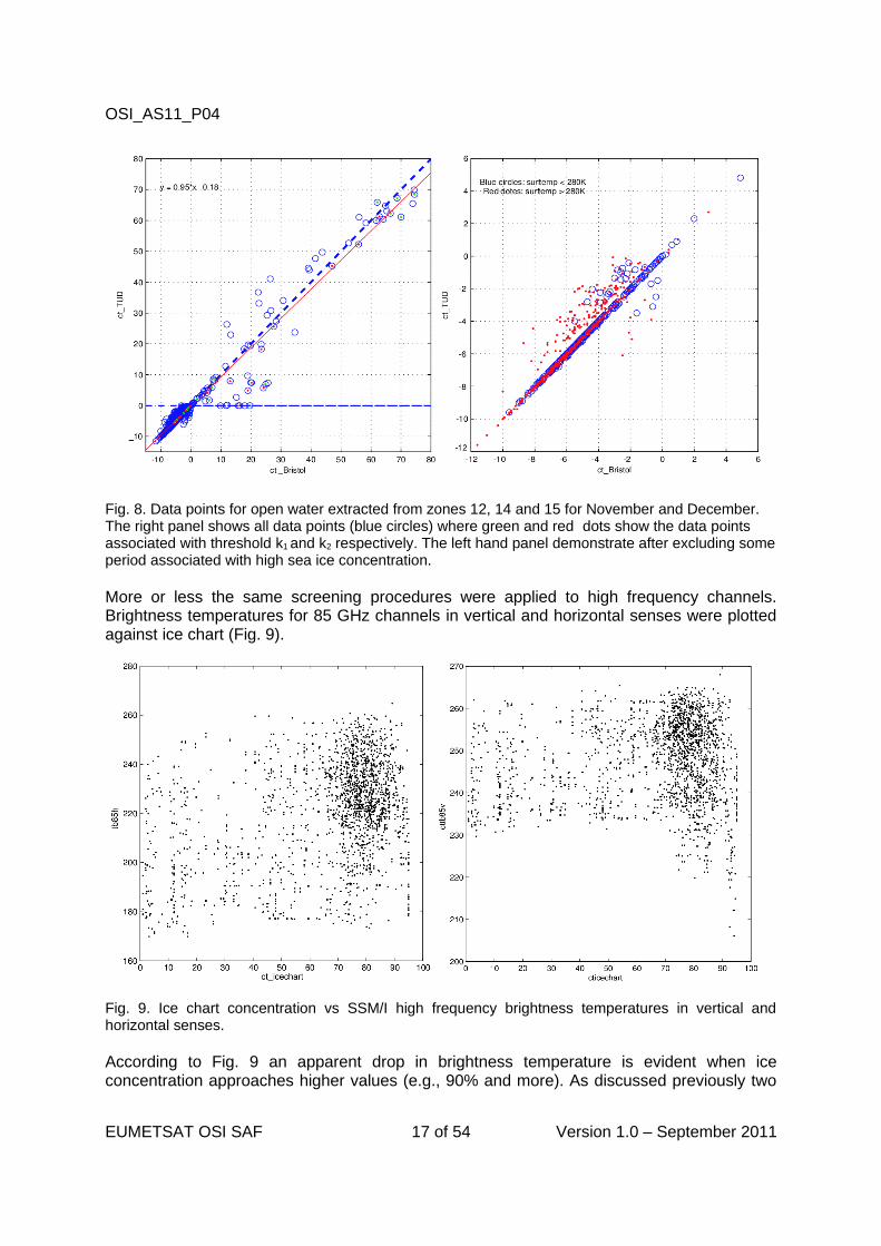
aimed to capturing the data points with not that much high surface temperature the remaining dataset was separated into two datasets based on the surface temperature higher and lower than 280 K (Fig. 8, left panel). Therefore the dataset associated with surface temperature lower than 280 K is considered as base dataset for open water tie-points (blue circles in left panel of Fig. 8).
EUMETSAT OSI SAF 16 of 54 Version 1.0 – September 2011
OSI_AS11_P04
Fig. 8. Data points for open water extracted from zones 12, 14 and 15 for November and December. The right panel shows all data points (blue circles) where green and red dots show the data points associated with threshold k1 and k2 respectively. The left hand panel demonstrate after excluding some period associated with high sea ice concentration.
More or less the same screening procedures were applied to high frequency channels. Brightness temperatures for 85 GHz channels in vertical and horizontal senses were plotted against ice chart (Fig. 9).
Fig. 9. Ice chart concentration vs SSM/I high frequency brightness temperatures in vertical and horizontal senses.
According to Fig. 9 an apparent drop in brightness temperature is evident when ice concentration approaches higher values (e.g., 90% and more). As discussed previously two
EUMETSAT OSI SAF 17 of 54 Version 1.0 – September 2011
OSI_AS11_P04
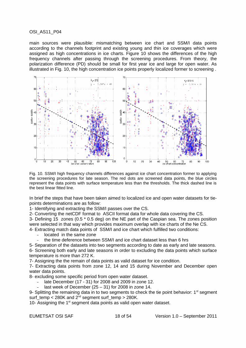
main sources were plausible: mismatching between ice chart and SSM/I data points according to the channels footprint and existing young and thin ice coverages which were assigned as high concentrations in ice charts. Figure 10 shows the differences of the high frequency channels after passing through the screening procedures. From theory, the polarization difference (PD) should be small for first year ice and large for open water. As illustrated in Fig. 10, the high concentration ice points properly localized former to screening .
Fig. 10. SSM/I high frequency channels differences against ice chart concentration former to applying the screening procedures for late season. The red dots are screened data points, the blue circles represent the data points with surface temperature less than the thresholds. The thick dashed line is the best linear fitted line. In brief the steps that have been taken aimed to localized ice and open water datasets for tie-points determinations are as follow:1- Identifying and extracting the SSM/I passes over the CS.2- Converting the netCDF format to ASCII format data for whole data covering the CS.3- Defining 15 zones (0.5 * 0.5 deg) on the NE part of the Caspian sea. The zones position were selected in that way which provides maximum overlap with ice charts of the Ne CS. 4- Extracting match data points of SSM/I and ice chart which fulfilled two conditions:
– located in the same zone– the time deference between SSM/I and ice chart dataset less than 6 hrs
5- Separation of the datasets into two segments according to date as early and late seasons.6- Screening both early and late seasons in order to excluding the data points which surface temperature is more than 272 K.7- Assigning the the remain of data points as valid dataset for ice condition. 7- Extracting data points from zone 12, 14 and 15 during November and December open water data points. 8- excluding some specific period from open water dataset.
– late December (17 - 31) for 2008 and 2009 in zone 12.– last week of December (25 – 31) for 2008 in zone 14.
9- Splitting the remaining data in to two segments to check the tie point behavior: 1st segment surf_temp < 280K and 2nd segment surf_temp > 280K.10- Assigning the 1st segment data points as valid open water dataset.
EUMETSAT OSI SAF 18 of 54 Version 1.0 – September 2011

OSI_AS11_P04
Data points from rectangles 12, 14 and 15 during November and December were used for open water tie points. We expected to see open water conditions on those two months with low surface temperature values and not that much different from ice conditions months. According to the ice charts and surface temperature there were some ice condition periods specially in rectangles number 12 and 14 that eliminated from data set. The eliminated periods from open water data sets:
1. late December (17 - 31) for 2008 and 2009 in zone 12.2. last week of December (25 – 31) for 2008 in zone 14.
additionally the remaining data were spited in to two segments to check the tie point behavior: 1st segment surf_temp < 280K and 2nd segment surf_temp > 280K.The final open water tie points were calculated based on 1st segment data points.
EUMETSAT OSI SAF 19 of 54 Version 1.0 – September 2011
OSI_AS11_P04
4. Tie-points (SSM/I)
4.1 Open water tie-points for the CS
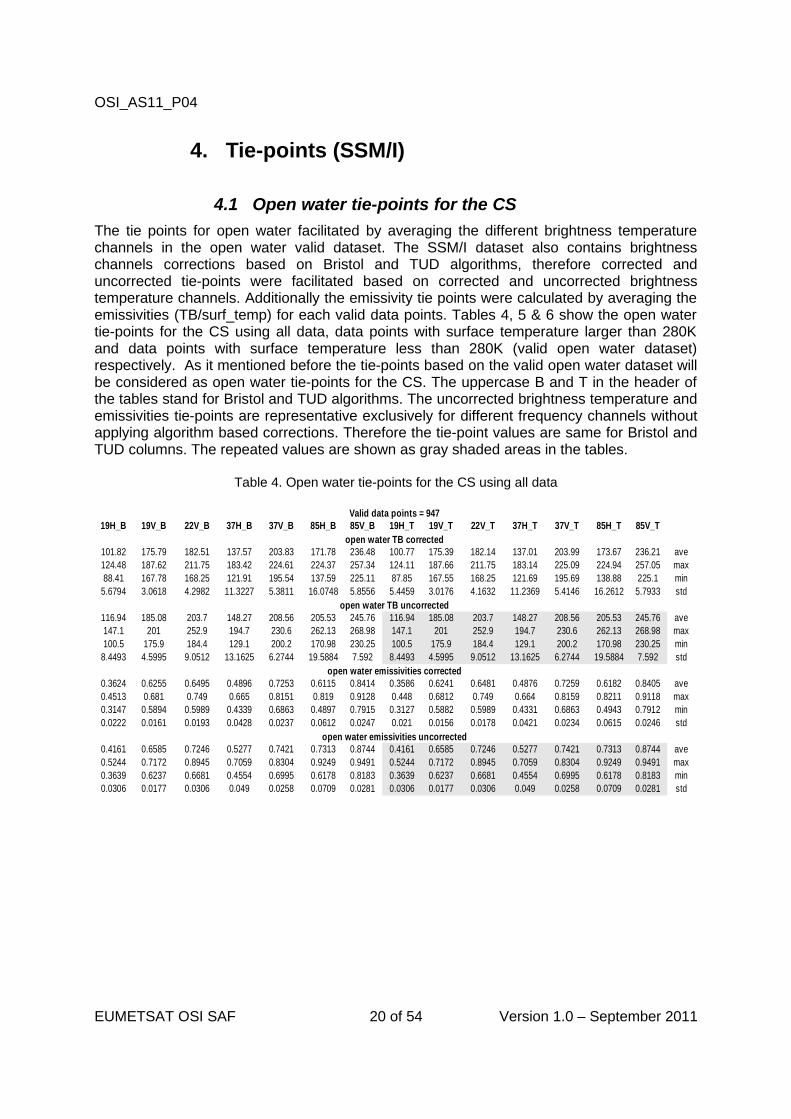
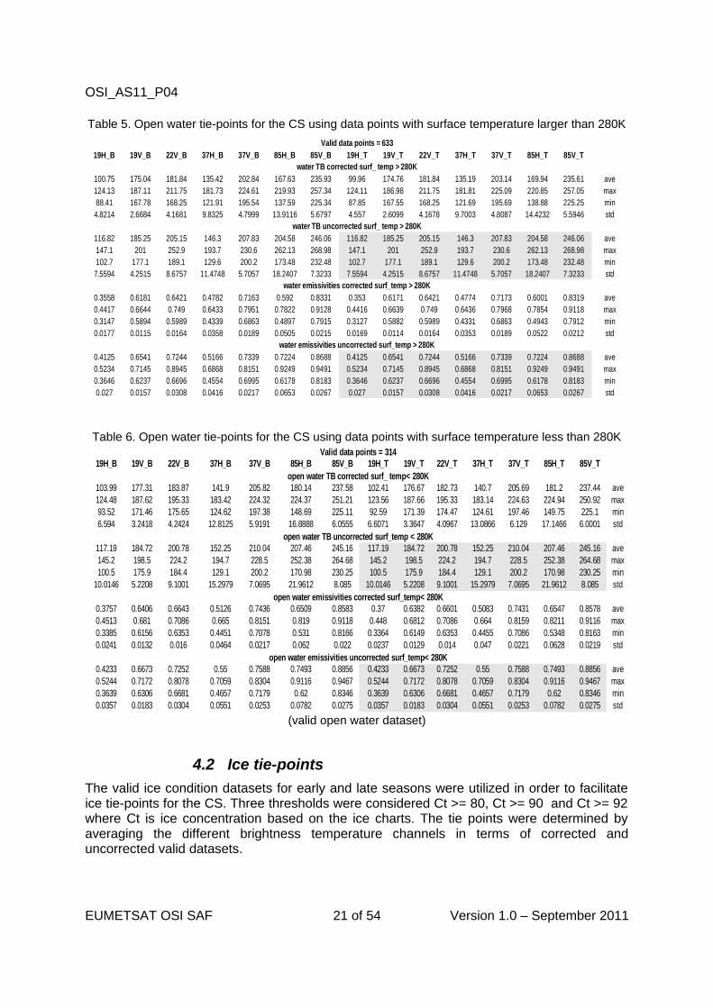
The tie points for open water facilitated by averaging the different brightness temperature channels in the open water valid dataset. The SSM/I dataset also contains brightness channels corrections based on Bristol and TUD algorithms, therefore corrected and uncorrected tie-points were facilitated based on corrected and uncorrected brightness temperature channels. Additionally the emissivity tie points were calculated by averaging the emissivities (TB/surf_temp) for each valid data points. Tables 4, 5 & 6 show the open water tie-points for the CS using all data, data points with surface temperature larger than 280K and data points with surface temperature less than 280K (valid open water dataset) respectively. As it mentioned before the tie-points based on the valid open water dataset will be considered as open water tie-points for the CS. The uppercase B and T in the header of the tables stand for Bristol and TUD algorithms. The uncorrected brightness temperature and emissivities tie-points are representative exclusively for different frequency channels without applying algorithm based corrections. Therefore the tie-point values are same for Bristol and TUD columns. The repeated values are shown as gray shaded areas in the tables.
Table 4. Open water tie-points for the CS using all data
EUMETSAT OSI SAF 20 of 54 Version 1.0 – September 2011
Valid data points = 94719H_B 19V_B 22V_B 37H_B 37V_B 85H_B 85V_B 19H_T 19V_T 22V_T 37H_T 37V_T 85H_T 85V_T
open water TB corrected101.82 175.79 182.51 137.57 203.83 171.78 236.48 100.77 175.39 182.14 137.01 203.99 173.67 236.21 ave124.48 187.62 211.75 183.42 224.61 224.37 257.34 124.11 187.66 211.75 183.14 225.09 224.94 257.05 max88.41 167.78 168.25 121.91 195.54 137.59 225.11 87.85 167.55 168.25 121.69 195.69 138.88 225.1 min
5.6794 3.0618 4.2982 11.3227 5.3811 16.0748 5.8556 5.4459 3.0176 4.1632 11.2369 5.4146 16.2612 5.7933 stdopen water TB uncorrected
116.94 185.08 203.7 148.27 208.56 205.53 245.76 116.94 185.08 203.7 148.27 208.56 205.53 245.76 ave147.1 201 252.9 194.7 230.6 262.13 268.98 147.1 201 252.9 194.7 230.6 262.13 268.98 max100.5 175.9 184.4 129.1 200.2 170.98 230.25 100.5 175.9 184.4 129.1 200.2 170.98 230.25 min
8.4493 4.5995 9.0512 13.1625 6.2744 19.5884 7.592 8.4493 4.5995 9.0512 13.1625 6.2744 19.5884 7.592 stdopen water emissivities corrected
0.3624 0.6255 0.6495 0.4896 0.7253 0.6115 0.8414 0.3586 0.6241 0.6481 0.4876 0.7259 0.6182 0.8405 ave0.4513 0.681 0.749 0.665 0.8151 0.819 0.9128 0.448 0.6812 0.749 0.664 0.8159 0.8211 0.9118 max0.3147 0.5894 0.5989 0.4339 0.6863 0.4897 0.7915 0.3127 0.5882 0.5989 0.4331 0.6863 0.4943 0.7912 min0.0222 0.0161 0.0193 0.0428 0.0237 0.0612 0.0247 0.021 0.0156 0.0178 0.0421 0.0234 0.0615 0.0246 std
open water emissivities uncorrected0.4161 0.6585 0.7246 0.5277 0.7421 0.7313 0.8744 0.4161 0.6585 0.7246 0.5277 0.7421 0.7313 0.8744 ave0.5244 0.7172 0.8945 0.7059 0.8304 0.9249 0.9491 0.5244 0.7172 0.8945 0.7059 0.8304 0.9249 0.9491 max0.3639 0.6237 0.6681 0.4554 0.6995 0.6178 0.8183 0.3639 0.6237 0.6681 0.4554 0.6995 0.6178 0.8183 min0.0306 0.0177 0.0306 0.049 0.0258 0.0709 0.0281 0.0306 0.0177 0.0306 0.049 0.0258 0.0709 0.0281 std
OSI_AS11_P04
Table 5. Open water tie-points for the CS using data points with surface temperature larger than 280K
Table 6. Open water tie-points for the CS using data points with surface temperature less than 280K
(valid open water dataset)
4.2 Ice tie-points
The valid ice condition datasets for early and late seasons were utilized in order to facilitate ice tie-points for the CS. Three thresholds were considered Ct >= 80, Ct >= 90 and Ct >= 92 where Ct is ice concentration based on the ice charts. The tie points were determined by averaging the different brightness temperature channels in terms of corrected and uncorrected valid datasets.
EUMETSAT OSI SAF 21 of 54 Version 1.0 – September 2011
Valid data points = 633
19H_B 19V_B 22V_B 37H_B 37V_B 85H_B 85V_B 19H_T 19V_T 22V_T 37H_T 37V_T 85H_T 85V_Twater TB corrected surf_ temp > 280K
100.75 175.04 181.84 135.42 202.84 167.63 235.93 99.96 174.76 181.84 135.19 203.14 169.94 235.61 ave124.13 187.11 211.75 181.73 224.61 219.93 257.34 124.11 186.98 211.75 181.81 225.09 220.85 257.05 max88.41 167.78 168.25 121.91 195.54 137.59 225.34 87.85 167.55 168.25 121.69 195.69 138.88 225.25 min
4.8214 2.6684 4.1681 9.8325 4.7999 13.9116 5.6797 4.557 2.6099 4.1678 9.7003 4.8087 14.4232 5.5946 stdwater TB uncorrected surf_ temp > 280K
116.82 185.25 205.15 146.3 207.83 204.58 246.06 116.82 185.25 205.15 146.3 207.83 204.58 246.06 ave147.1 201 252.9 193.7 230.6 262.13 268.98 147.1 201 252.9 193.7 230.6 262.13 268.98 max102.7 177.1 189.1 129.6 200.2 173.48 232.48 102.7 177.1 189.1 129.6 200.2 173.48 232.48 min
7.5594 4.2515 8.6757 11.4748 5.7057 18.2407 7.3233 7.5594 4.2515 8.6757 11.4748 5.7057 18.2407 7.3233 stdwater emissivities corrected surf_temp > 280K
0.3558 0.6181 0.6421 0.4782 0.7163 0.592 0.8331 0.353 0.6171 0.6421 0.4774 0.7173 0.6001 0.8319 ave0.4417 0.6644 0.749 0.6433 0.7951 0.7822 0.9128 0.4416 0.6639 0.749 0.6436 0.7968 0.7854 0.9118 max0.3147 0.5894 0.5989 0.4339 0.6863 0.4897 0.7915 0.3127 0.5882 0.5989 0.4331 0.6863 0.4943 0.7912 min0.0177 0.0115 0.0164 0.0358 0.0189 0.0505 0.0215 0.0169 0.0114 0.0164 0.0353 0.0189 0.0522 0.0212 std
water emissivities uncorrected surf_temp > 280K
0.4125 0.6541 0.7244 0.5166 0.7339 0.7224 0.8688 0.4125 0.6541 0.7244 0.5166 0.7339 0.7224 0.8688 ave0.5234 0.7145 0.8945 0.6868 0.8151 0.9249 0.9491 0.5234 0.7145 0.8945 0.6868 0.8151 0.9249 0.9491 max0.3646 0.6237 0.6696 0.4554 0.6995 0.6178 0.8183 0.3646 0.6237 0.6696 0.4554 0.6995 0.6178 0.8183 min0.027 0.0157 0.0308 0.0416 0.0217 0.0653 0.0267 0.027 0.0157 0.0308 0.0416 0.0217 0.0653 0.0267 std
Valid data points = 31419H_B 19V_B 22V_B 37H_B 37V_B 85H_B 85V_B 19H_T 19V_T 22V_T 37H_T 37V_T 85H_T 85V_T
open water TB corrected surf_ temp< 280K103.99 177.31 183.87 141.9 205.82 180.14 237.58 102.41 176.67 182.73 140.7 205.69 181.2 237.44 ave124.48 187.62 195.33 183.42 224.32 224.37 251.21 123.56 187.66 195.33 183.14 224.63 224.94 250.92 max93.52 171.46 175.65 124.62 197.38 148.69 225.11 92.59 171.39 174.47 124.61 197.46 149.75 225.1 min6.594 3.2418 4.2424 12.8125 5.9191 16.8888 6.0555 6.6071 3.3647 4.0967 13.0866 6.129 17.1466 6.0001 std
open water TB uncorrected surf_temp < 280K117.19 184.72 200.78 152.25 210.04 207.46 245.16 117.19 184.72 200.78 152.25 210.04 207.46 245.16 ave145.2 198.5 224.2 194.7 228.5 252.38 264.68 145.2 198.5 224.2 194.7 228.5 252.38 264.68 max100.5 175.9 184.4 129.1 200.2 170.98 230.25 100.5 175.9 184.4 129.1 200.2 170.98 230.25 min
10.0146 5.2208 9.1001 15.2979 7.0695 21.9612 8.085 10.0146 5.2208 9.1001 15.2979 7.0695 21.9612 8.085 stdopen water emissivities corrected surf_temp< 280K
0.3757 0.6406 0.6643 0.5126 0.7436 0.6509 0.8583 0.37 0.6382 0.6601 0.5083 0.7431 0.6547 0.8578 ave0.4513 0.681 0.7086 0.665 0.8151 0.819 0.9118 0.448 0.6812 0.7086 0.664 0.8159 0.8211 0.9116 max0.3385 0.6156 0.6353 0.4451 0.7078 0.531 0.8166 0.3364 0.6149 0.6353 0.4455 0.7086 0.5348 0.8163 min0.0241 0.0132 0.016 0.0464 0.0217 0.062 0.022 0.0237 0.0129 0.014 0.047 0.0221 0.0628 0.0219 std
open water emissivities uncorrected surf_temp< 280K0.4233 0.6673 0.7252 0.55 0.7588 0.7493 0.8856 0.4233 0.6673 0.7252 0.55 0.7588 0.7493 0.8856 ave0.5244 0.7172 0.8078 0.7059 0.8304 0.9116 0.9467 0.5244 0.7172 0.8078 0.7059 0.8304 0.9116 0.9467 max0.3639 0.6306 0.6681 0.4657 0.7179 0.62 0.8346 0.3639 0.6306 0.6681 0.4657 0.7179 0.62 0.8346 min0.0357 0.0183 0.0304 0.0551 0.0253 0.0782 0.0275 0.0357 0.0183 0.0304 0.0551 0.0253 0.0782 0.0275 std
OSI_AS11_P04
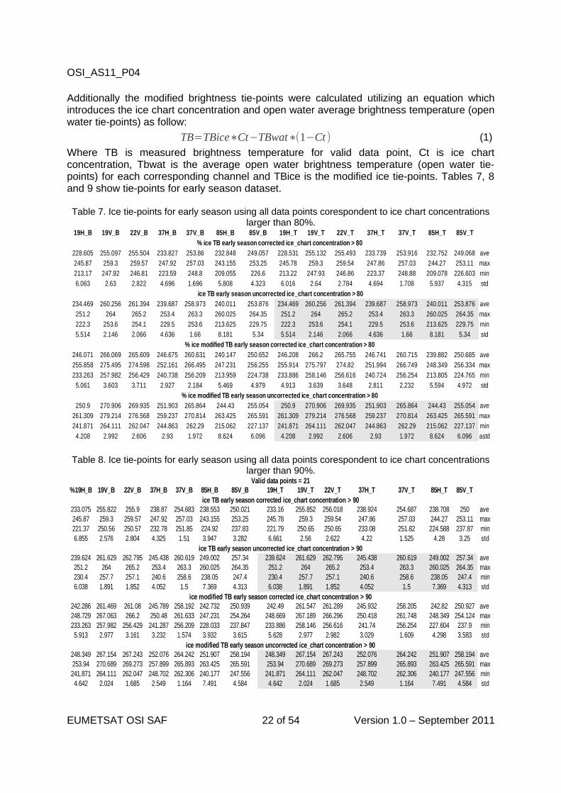
Additionally the modified brightness tie-points were calculated utilizing an equation which introduces the ice chart concentration and open water average brightness temperature (open water tie-points) as follow:
TB=TBice∗Ct−TBwat∗(1−Ct ) (1)
Where TB is measured brightness temperature for valid data point, Ct is ice chart concentration, Tbwat is the average open water brightness temperature (open water tie-points) for each corresponding channel and TBice is the modified ice tie-points. Tables 7, 8 and 9 show tie-points for early season dataset.
Table 7. Ice tie-points for early season using all data points corespondent to ice chart concentrations larger than 80%.
Table 8. Ice tie-points for early season using all data points corespondent to ice chart concentrations larger than 90%.
EUMETSAT OSI SAF 22 of 54 Version 1.0 – September 2011
19H_B 19V_B 22V_B 37H_B 37V_B 85H_B 85V_B 19H_T 19V_T 22V_T 37H_T 37V_T 85H_T 85V_T
% ice TB early season corrected ice_chart concentration > 80
228.605 255.097 255.504 233.827 253.86 232.848 249.057 228.531 255.132 255.493 233.739 253.916 232.752 249.068 ave245.87 259.3 259.57 247.92 257.03 243.155 253.25 245.78 259.3 259.54 247.86 257.03 244.27 253.11 max
213.17 247.92 246.81 223.59 248.8 209.055 226.6 213.22 247.93 246.86 223.37 248.88 209.078 226.603 min
6.063 2.63 2.822 4.696 1.696 5.808 4.323 6.016 2.64 2.784 4.694 1.708 5.937 4.315 std
ice TB early season uncorrected ice_chart concentration > 80
234.469 260.256 261.394 239.687 258.973 240.011 253.876 234.469 260.256 261.394 239.687 258.973 240.011 253.876 ave
251.2 264 265.2 253.4 263.3 260.025 264.35 251.2 264 265.2 253.4 263.3 260.025 264.35 max
222.3 253.6 254.1 229.5 253.6 213.625 229.75 222.3 253.6 254.1 229.5 253.6 213.625 229.75 min
5.514 2.146 2.066 4.636 1.66 8.181 5.34 5.514 2.146 2.066 4.636 1.66 8.181 5.34 std
% ice modified TB early season corrected ice_chart concentration > 80
246.071 266.069 265.609 246.675 260.631 240.147 250.652 246.208 266.2 265.755 246.741 260.715 239.882 250.685 ave
255.858 275.495 274.598 252.161 266.495 247.231 256.255 255.914 275.797 274.82 251.994 266.749 248.349 256.334 max
233.263 257.982 256.429 240.738 256.209 213.959 224.738 233.886 258.146 256.616 240.724 256.254 213.805 224.765 min
5.061 3.603 3.711 2.927 2.184 5.469 4.979 4.913 3.639 3.648 2.811 2.232 5.594 4.972 std
% ice modified TB early season uncorrected ice_chart concentration > 80250.9 270.906 269.935 251.903 265.864 244.43 255.054 250.9 270.906 269.935 251.903 265.864 244.43 255.054 ave
261.309 279.214 276.568 259.237 270.814 263.425 265.591 261.309 279.214 276.568 259.237 270.814 263.425 265.591 max
241.871 264.111 262.047 244.863 262.29 215.062 227.137 241.871 264.111 262.047 244.863 262.29 215.062 227.137 min
4.208 2.992 2.606 2.93 1.972 8.624 6.096 4.208 2.992 2.606 2.93 1.972 8.624 6.096 astd
Valid data points = 21%19H_B 19V_B 22V_B 37H_B 37V_B 85H_B 85V_B 19H_T 19V_T 22V_T 37H_T 37V_T 85H_T 85V_T
ice TB early season corrected ice_chart concentration > 90233.075 255.822 255.9 238.87 254.683 238.553 250.021 233.16 255.852 256.018 238.924 254.687 238.708 250 ave 245.87 259.3 259.57 247.92 257.03 243.155 253.25 245.78 259.3 259.54 247.86 257.03 244.27 253.11 max221.37 250.56 250.57 232.78 251.85 224.92 237.83 221.79 250.65 250.65 233.08 251.82 224.588 237.87 min6.855 2.576 2.804 4.325 1.51 3.947 3.282 6.661 2.56 2.622 4.22 1.525 4.28 3.25 std
ice TB early season uncorrected ice_chart concentration > 90239.624 261.629 262.795 245.438 260.619 249.002 257.34 239.624 261.629 262.795 245.438 260.619 249.002 257.34 ave 251.2 264 265.2 253.4 263.3 260.025 264.35 251.2 264 265.2 253.4 263.3 260.025 264.35 max230.4 257.7 257.1 240.6 258.6 238.05 247.4 230.4 257.7 257.1 240.6 258.6 238.05 247.4 min6.038 1.891 1.852 4.052 1.5 7.369 4.313 6.038 1.891 1.852 4.052 1.5 7.369 4.313 std
ice modified TB early season corrected ice_chart concentration > 90242.286 261.469 261.08 245.789 258.192 242.732 250.939 242.49 261.547 261.289 245.932 258.205 242.82 250.927 ave 248.729 267.063 266.2 250.48 261.633 247.231 254.264 248.669 267.189 266.296 250.418 261.748 248.349 254.124 max233.263 257.982 256.429 241.287 256.209 228.033 237.847 233.886 258.146 256.616 241.74 256.254 227.604 237.9 min5.913 2.977 3.161 3.232 1.574 3.932 3.615 5.628 2.977 2.982 3.029 1.609 4.298 3.583 std
ice modified TB early season uncorrected ice_chart concentration > 90248.349 267.154 267.243 252.076 264.242 251.907 258.194 248.349 267.154 267.243 252.076 264.242 251.907 258.194 ave 253.94 270.689 269.273 257.899 265.893 263.425 265.591 253.94 270.689 269.273 257.899 265.893 263.425 265.591 max241.871 264.111 262.047 248.702 262.306 240.177 247.556 241.871 264.111 262.047 248.702 262.306 240.177 247.556 min4.642 2.024 1.685 2.549 1.164 7.491 4.584 4.642 2.024 1.685 2.549 1.164 7.491 4.584 std
OSI_AS11_P04
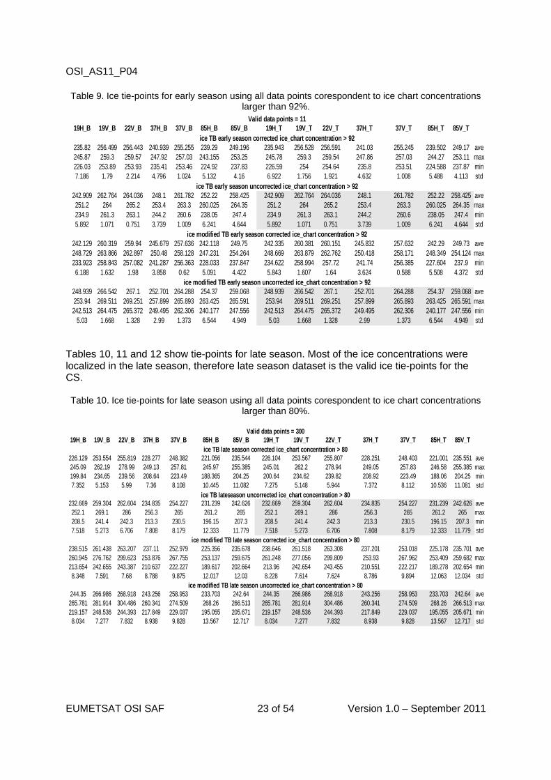
Table 9. Ice tie-points for early season using all data points corespondent to ice chart concentrations larger than 92%.
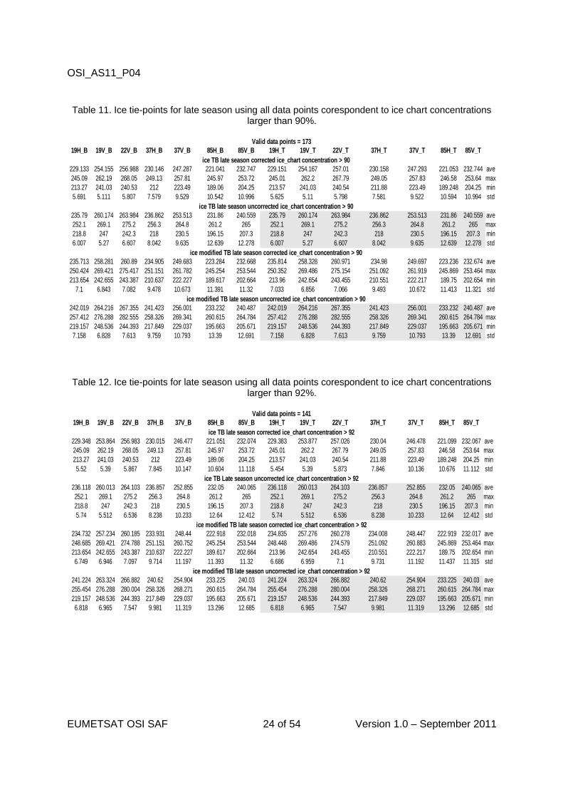
Tables 10, 11 and 12 show tie-points for late season. Most of the ice concentrations were localized in the late season, therefore late season dataset is the valid ice tie-points for the CS.
Table 10. Ice tie-points for late season using all data points corespondent to ice chart concentrations larger than 80%.
EUMETSAT OSI SAF 23 of 54 Version 1.0 – September 2011
Valid data points = 1119H_B 19V_B 22V_B 37H_B 37V_B 85H_B 85V_B 19H_T 19V_T 22V_T 37H_T 37V_T 85H_T 85V_T
ice TB early season corrected ice_chart concentration > 92235.82 256.499 256.443 240.939 255.255 239.29 249.196 235.943 256.528 256.591 241.03 255.245 239.502 249.17 ave245.87 259.3 259.57 247.92 257.03 243.155 253.25 245.78 259.3 259.54 247.86 257.03 244.27 253.11 max226.03 253.89 253.93 235.41 253.46 224.92 237.83 226.59 254 254.64 235.8 253.51 224.588 237.87 min7.186 1.79 2.214 4.796 1.024 5.132 4.16 6.922 1.756 1.921 4.632 1.008 5.488 4.113 std
ice TB early season uncorrected ice_chart concentration > 92242.909 262.764 264.036 248.1 261.782 252.22 258.425 242.909 262.764 264.036 248.1 261.782 252.22 258.425 ave251.2 264 265.2 253.4 263.3 260.025 264.35 251.2 264 265.2 253.4 263.3 260.025 264.35 max234.9 261.3 263.1 244.2 260.6 238.05 247.4 234.9 261.3 263.1 244.2 260.6 238.05 247.4 min5.892 1.071 0.751 3.739 1.009 6.241 4.644 5.892 1.071 0.751 3.739 1.009 6.241 4.644 std
ice modified TB early season corrected ice_chart concentration > 92242.129 260.319 259.94 245.679 257.636 242.118 249.75 242.335 260.381 260.151 245.832 257.632 242.29 249.73 ave248.729 263.866 262.897 250.48 258.128 247.231 254.264 248.669 263.879 262.762 250.418 258.171 248.349 254.124 max233.923 258.843 257.082 241.287 256.363 228.033 237.847 234.622 258.994 257.72 241.74 256.385 227.604 237.9 min6.188 1.632 1.98 3.858 0.62 5.091 4.422 5.843 1.607 1.64 3.624 0.588 5.508 4.372 std
ice modified TB early season uncorrected ice_chart concentration > 92248.939 266.542 267.1 252.701 264.288 254.37 259.068 248.939 266.542 267.1 252.701 264.288 254.37 259.068 ave253.94 269.511 269.251 257.899 265.893 263.425 265.591 253.94 269.511 269.251 257.899 265.893 263.425 265.591 max242.513 264.475 265.372 249.495 262.306 240.177 247.556 242.513 264.475 265.372 249.495 262.306 240.177 247.556 min
5.03 1.668 1.328 2.99 1.373 6.544 4.949 5.03 1.668 1.328 2.99 1.373 6.544 4.949 std
Valid data points = 30019H_B 19V_B 22V_B 37H_B 37V_B 85H_B 85V_B 19H_T 19V_T 22V_T 37H_T 37V_T 85H_T 85V_T
ice TB late season corrected ice_chart concentration > 80226.129 253.554 255.819 228.277 248.382 221.056 235.544 226.104 253.567 255.807 228.251 248.403 221.001 235.551 ave245.09 262.19 278.99 249.13 257.81 245.97 255.385 245.01 262.2 278.94 249.05 257.83 246.58 255.385 max199.84 234.65 239.56 208.64 223.49 188.365 204.25 200.64 234.62 239.82 208.92 223.49 188.06 204.25 min7.352 5.153 5.99 7.36 8.108 10.445 11.082 7.275 5.148 5.944 7.372 8.112 10.536 11.081 std
232.669 259.304 262.604 234.835 254.227 231.239 242.626 232.669 259.304 262.604 234.835 254.227 231.239 242.626 ave252.1 269.1 286 256.3 265 261.2 265 252.1 269.1 286 256.3 265 261.2 265 max208.5 241.4 242.3 213.3 230.5 196.15 207.3 208.5 241.4 242.3 213.3 230.5 196.15 207.3 min7.518 5.273 6.706 7.808 8.179 12.333 11.779 7.518 5.273 6.706 7.808 8.179 12.333 11.779 std
ice modified TB late season corrected ice_chart concentration > 80238.515 261.438 263.207 237.11 252.979 225.356 235.678 238.646 261.518 263.308 237.201 253.018 225.178 235.701 ave260.945 276.762 299.623 253.876 267.755 253.137 259.675 261.248 277.056 299.809 253.93 267.962 253.409 259.682 max213.654 242.655 243.387 210.637 222.227 189.617 202.664 213.96 242.654 243.455 210.551 222.217 189.278 202.654 min8.348 7.591 7.68 8.788 9.875 12.017 12.03 8.228 7.614 7.624 8.786 9.894 12.063 12.034 std
ice modified TB late season uncorrected ice_chart concentration > 80244.35 266.986 268.918 243.256 258.953 233.703 242.64 244.35 266.986 268.918 243.256 258.953 233.703 242.64 ave265.781 281.914 304.486 260.341 274.509 268.26 266.513 265.781 281.914 304.486 260.341 274.509 268.26 266.513 max219.157 248.536 244.393 217.849 229.037 195.055 205.671 219.157 248.536 244.393 217.849 229.037 195.055 205.671 min8.034 7.277 7.832 8.938 9.828 13.567 12.717 8.034 7.277 7.832 8.938 9.828 13.567 12.717 std
ice TB lateseason uncorrected ice_chart concentration > 80
OSI_AS11_P04
Table 11. Ice tie-points for late season using all data points corespondent to ice chart concentrations larger than 90%.
Table 12. Ice tie-points for late season using all data points corespondent to ice chart concentrations larger than 92%.
EUMETSAT OSI SAF 24 of 54 Version 1.0 – September 2011
Valid data points = 17319H_B 19V_B 22V_B 37H_B 37V_B 85H_B 85V_B 19H_T 19V_T 22V_T 37H_T 37V_T 85H_T 85V_T
ice TB late season corrected ice_chart concentration > 90229.133 254.155 256.988 230.146 247.287 221.041 232.747 229.151 254.167 257.01 230.158 247.293 221.053 232.744 ave245.09 262.19 268.05 249.13 257.81 245.97 253.72 245.01 262.2 267.79 249.05 257.83 246.58 253.64 max213.27 241.03 240.53 212 223.49 189.06 204.25 213.57 241.03 240.54 211.88 223.49 189.248 204.25 min5.691 5.111 5.807 7.579 9.529 10.542 10.996 5.625 5.11 5.798 7.581 9.522 10.594 10.994 std
ice TB late season uncorrected ice_chart concentration > 90235.79 260.174 263.984 236.862 253.513 231.86 240.559 235.79 260.174 263.984 236.862 253.513 231.86 240.559 ave252.1 269.1 275.2 256.3 264.8 261.2 265 252.1 269.1 275.2 256.3 264.8 261.2 265 max218.8 247 242.3 218 230.5 196.15 207.3 218.8 247 242.3 218 230.5 196.15 207.3 min6.007 5.27 6.607 8.042 9.635 12.639 12.278 6.007 5.27 6.607 8.042 9.635 12.639 12.278 std
ice modified TB late season corrected ice_chart concentration > 90235.713 258.281 260.89 234.905 249.683 223.284 232.668 235.814 258.328 260.971 234.98 249.697 223.236 232.674 ave250.424 269.421 275.417 251.151 261.782 245.254 253.544 250.352 269.486 275.154 251.092 261.919 245.869 253.464 max213.654 242.655 243.387 210.637 222.227 189.617 202.664 213.96 242.654 243.455 210.551 222.217 189.75 202.654 min
7.1 6.843 7.082 9.478 10.673 11.391 11.32 7.033 6.856 7.066 9.493 10.672 11.413 11.321 stdice modified TB late season uncorrected ice_chart concentration > 90
242.019 264.216 267.355 241.423 256.001 233.232 240.487 242.019 264.216 267.355 241.423 256.001 233.232 240.487 ave257.412 276.288 282.555 258.326 269.341 260.615 264.784 257.412 276.288 282.555 258.326 269.341 260.615 264.784 max219.157 248.536 244.393 217.849 229.037 195.663 205.671 219.157 248.536 244.393 217.849 229.037 195.663 205.671 min7.158 6.828 7.613 9.759 10.793 13.39 12.691 7.158 6.828 7.613 9.759 10.793 13.39 12.691 std
Valid data points = 14119H_B 19V_B 22V_B 37H_B 37V_B 85H_B 85V_B 19H_T 19V_T 22V_T 37H_T 37V_T 85H_T 85V_T
ice TB late season corrected ice_chart concentration > 92229.348 253.864 256.983 230.015 246.477 221.051 232.074 229.383 253.877 257.026 230.04 246.478 221.099 232.067 ave245.09 262.19 268.05 249.13 257.81 245.97 253.72 245.01 262.2 267.79 249.05 257.83 246.58 253.64 max213.27 241.03 240.53 212 223.49 189.06 204.25 213.57 241.03 240.54 211.88 223.49 189.248 204.25 min5.52 5.39 5.867 7.845 10.147 10.604 11.118 5.454 5.39 5.873 7.846 10.136 10.676 11.112 std
ice TB Late season uncorrected ice_chart concentration > 92236.118 260.013 264.103 236.857 252.855 232.05 240.065 236.118 260.013 264.103 236.857 252.855 232.05 240.065 ave252.1 269.1 275.2 256.3 264.8 261.2 265 252.1 269.1 275.2 256.3 264.8 261.2 265 max218.8 247 242.3 218 230.5 196.15 207.3 218.8 247 242.3 218 230.5 196.15 207.3 min5.74 5.512 6.536 8.238 10.233 12.64 12.412 5.74 5.512 6.536 8.238 10.233 12.64 12.412 std
ice modified TB late season corrected ice_chart concentration > 92234.732 257.234 260.185 233.931 248.44 222.918 232.018 234.835 257.276 260.278 234.008 248.447 222.919 232.017 ave248.685 269.421 274.788 251.151 260.752 245.254 253.544 248.448 269.486 274.579 251.092 260.883 245.869 253.464 max213.654 242.655 243.387 210.637 222.227 189.617 202.664 213.96 242.654 243.455 210.551 222.217 189.75 202.654 min6.749 6.946 7.097 9.714 11.197 11.393 11.32 6.686 6.959 7.1 9.731 11.192 11.437 11.315 std
ice modified TB late season uncorrected ice_chart concentration > 92241.224 263.324 266.882 240.62 254.904 233.225 240.03 241.224 263.324 266.882 240.62 254.904 233.225 240.03 ave255.454 276.288 280.004 258.326 268.271 260.615 264.784 255.454 276.288 280.004 258.326 268.271 260.615 264.784 max219.157 248.536 244.393 217.849 229.037 195.663 205.671 219.157 248.536 244.393 217.849 229.037 195.663 205.671 min6.818 6.965 7.547 9.981 11.319 13.296 12.685 6.818 6.965 7.547 9.981 11.319 13.296 12.685 std
OSI_AS11_P04
5. Sea Ice retrieval algorithms (SSM/I)
5.1 Bristol algorithm
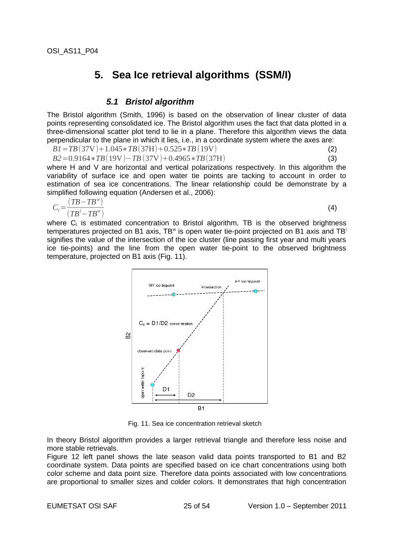
The Bristol algorithm (Smith, 1996) is based on the observation of linear cluster of data points representing consolidated ice. The Bristol algorithm uses the fact that data plotted in a three-dimensional scatter plot tend to lie in a plane. Therefore this algorithm views the data perpendicular to the plane in which it lies, i.e., in a coordinate system where the axes are:B1=TB(37V )+1.045∗TB(37H)+0.525∗TB (19V) (2)B2=0.9164∗TB(19V)−TB (37V)+0.4965∗TB(37H) (3)
where H and V are horizontal and vertical polarizations respectively. In this algorithm the variability of surface ice and open water tie points are tacking to account in order to estimation of sea ice concentrations. The linear relationship could be demonstrate by a simplified following equation (Andersen et al., 2006):
Ct=(TB−TBw)
(TB i−TBw
)(4)
where Ct is estimated concentration to Bristol algorithm, TB is the observed brightness temperatures projected on B1 axis, TBw is open water tie-point projected on B1 axis and TB i
signifies the value of the intersection of the ice cluster (line passing first year and multi years ice tie-points) and the line from the open water tie-point to the observed brightness temperature, projected on B1 axis (Fig. 11).
Fig. 11. Sea ice concentration retrieval sketch
In theory Bristol algorithm provides a larger retrieval triangle and therefore less noise and more stable retrievals.Figure 12 left panel shows the late season valid data points transported to B1 and B2 coordinate system. Data points are specified based on ice chart concentrations using both color scheme and data point size. Therefore data points associated with low concentrations are proportional to smaller sizes and colder colors. It demonstrates that high concentration
EUMETSAT OSI SAF 25 of 54 Version 1.0 – September 2011
OSI_AS11_P04
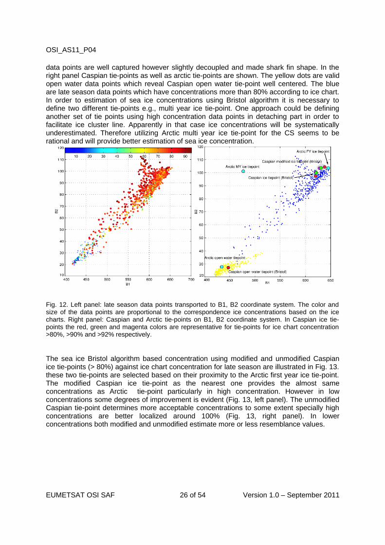
data points are well captured however slightly decoupled and made shark fin shape. In the right panel Caspian tie-points as well as arctic tie-points are shown. The yellow dots are valid open water data points which reveal Caspian open water tie-point well centered. The blue are late season data points which have concentrations more than 80% according to ice chart. In order to estimation of sea ice concentrations using Bristol algorithm it is necessary to define two different tie-points e.g., multi year ice tie-point. One approach could be defining another set of tie points using high concentration data points in detaching part in order to facilitate ice cluster line. Apparently in that case ice concentrations will be systematically underestimated. Therefore utilizing Arctic multi year ice tie-point for the CS seems to be rational and will provide better estimation of sea ice concentration.
Fig. 12. Left panel: late season data points transported to B1, B2 coordinate system. The color and size of the data points are proportional to the correspondence ice concentrations based on the ice charts. Right panel: Caspian and Arctic tie-points on B1, B2 coordinate system. In Caspian ice tie-points the red, green and magenta colors are representative for tie-points for ice chart concentration >80%, >90% and >92% respectively.
The sea ice Bristol algorithm based concentration using modified and unmodified Caspian ice tie-points (> 80%) against ice chart concentration for late season are illustrated in Fig. 13. these two tie-points are selected based on their proximity to the Arctic first year ice tie-point. The modified Caspian ice tie-point as the nearest one provides the almost same concentrations as Arctic tie-point particularly in high concentration. However in low concentrations some degrees of improvement is evident (Fig. 13, left panel). The unmodified Caspian tie-point determines more acceptable concentrations to some extent specially high concentrations are better localized around 100% (Fig. 13, right panel). In lower concentrations both modified and unmodified estimate more or less resemblance values.
EUMETSAT OSI SAF 26 of 54 Version 1.0 – September 2011
OSI_AS11_P04
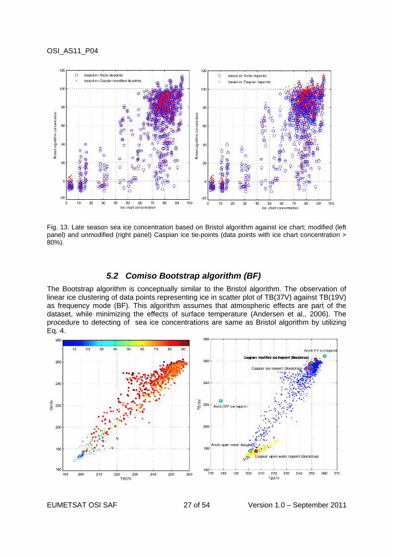
Fig. 13. Late season sea ice concentration based on Bristol algorithm against ice chart; modified (left panel) and unmodified (right panel) Caspian ice tie-points (data points with ice chart concentration > 80%).
5.2 Comiso Bootstrap algorithm (BF)
The Bootstrap algorithm is conceptually similar to the Bristol algorithm. The observation of linear ice clustering of data points representing ice in scatter plot of TB(37V) against TB(19V) as frequency mode (BF). This algorithm assumes that atmospheric effects are part of the dataset, while minimizing the effects of surface temperature (Andersen et al., 2006). The procedure to detecting of sea ice concentrations are same as Bristol algorithm by utilizing Eq. 4.
EUMETSAT OSI SAF 27 of 54 Version 1.0 – September 2011
OSI_AS11_P04
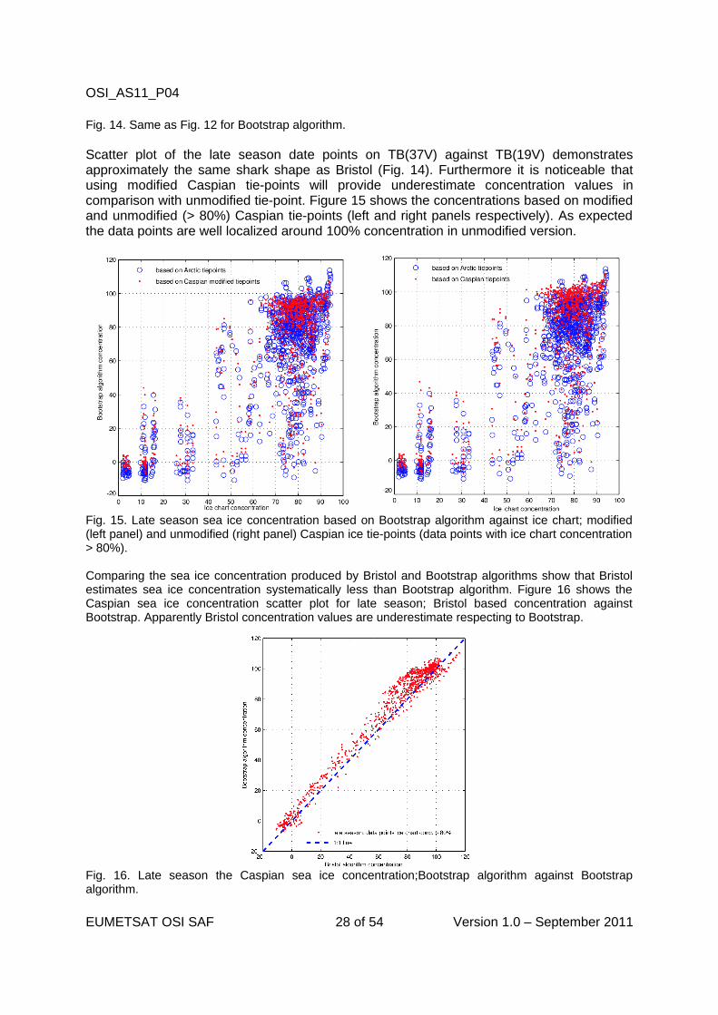
Fig. 14. Same as Fig. 12 for Bootstrap algorithm.
Scatter plot of the late season date points on TB(37V) against TB(19V) demonstrates approximately the same shark shape as Bristol (Fig. 14). Furthermore it is noticeable that using modified Caspian tie-points will provide underestimate concentration values in comparison with unmodified tie-point. Figure 15 shows the concentrations based on modified and unmodified (> 80%) Caspian tie-points (left and right panels respectively). As expected the data points are well localized around 100% concentration in unmodified version.
Fig. 15. Late season sea ice concentration based on Bootstrap algorithm against ice chart; modified (left panel) and unmodified (right panel) Caspian ice tie-points (data points with ice chart concentration > 80%).
Comparing the sea ice concentration produced by Bristol and Bootstrap algorithms show that Bristol estimates sea ice concentration systematically less than Bootstrap algorithm. Figure 16 shows the Caspian sea ice concentration scatter plot for late season; Bristol based concentration against Bootstrap. Apparently Bristol concentration values are underestimate respecting to Bootstrap.
Fig. 16. Late season the Caspian sea ice concentration;Bootstrap algorithm against Bootstrap algorithm.
EUMETSAT OSI SAF 28 of 54 Version 1.0 – September 2011
OSI_AS11_P04
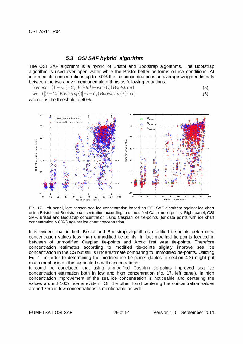
5.3 OSI SAF hybrid algorithm
The OSI SAF algorithm is a hybrid of Bristol and Bootstrap algorithms. The Bootstrap algorithm is used over open water while the Bristol better performs on ice conditions. At intermediate concentrations up to 40% the ice concentration is an average weighted linearly between the two above mentioned algorithms as following equations:iceconc=(1−wc)∗C t(Bristol)+wc∗C t(Bootstrap) (5)wc=(∣(t−Ct (Bootstrap))∣+t−Ct (Bootstrap))/(2∗t ) (6)
where t is the threshold of 40%.
Fig. 17. Left panel, late season sea ice concentration based on OSI SAF algorithm against ice chart using Bristol and Bootstrap concentration according to unmodified Caspian tie-points. Right panel, OSI SAF, Bristol and Bootstrap concentration using Caspian ice tie-points (for data points with ice chart concentration > 80%) against ice chart concentration.
It is evident that in both Bristol and Bootstrap algorithms modified tie-points determined concentration values less than unmodified tie-points. In fact modified tie-points located in between of unmodified Caspian tie-points and Arctic first year tie-points. Therefore concentration estimates according to modified tie-points slightly improve sea ice concentration in the CS but still is underestimate comparing to unmodified tie-points. Utilizing Eq. 1 in order to determining the modified ice tie-points (tables in section 4.2) might put much emphasis on the suspected small concentrations. It could be concluded that using unmodified Caspian tie-points improved sea ice concentration estimation both in low and high concentration (fig. 17, left panel). In high concentration improvement of the sea ice concentration is noticeable and centering the values around 100% ice is evident. On the other hand centering the concentration values around zero in low concentrations is mentionable as well.
EUMETSAT OSI SAF 29 of 54 Version 1.0 – September 2011
OSI_AS11_P04
6. AMSR-E dataset
6.1 Data treating (AMSR-E)
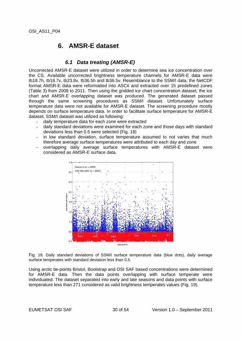
Uncorrected AMSR-E dataset were utilized in order to determine sea ice concentration over the CS. Available uncorrected brightness temperature channels for AMSR-E data were tb18.7h, tb18.7v, tb23.8v, tb36.5h and tb36.5v. Resemblance to the SSM/I data, the NetCDF format AMSR-E data were reformatted into ASCII and extracted over 15 predefined zones (Table 3) from 2008 to 2011. Then using the gridded ice chart concentration dataset, the ice chart and AMSR-E overlapping dataset was produced. The generated dataset passed through the same screening procedures as SSM/I dataset. Unfortunately surface temperature data were not available for AMSR-E dataset. The screening procedure mostly depends on surface temperature data. In order to facilitate surface temperature for AMSR-E dataset, SSM/I dataset was utilized as following:
– daily temperature data for each zone were extracted– daily standard deviations were examined for each zone and those days with standard
deviations less than 0.5 were selected (Fig. 18)– in low standard deviation, surface temperature assumed to not varies that much
therefore average surface temperatures were attributed to each day and zone – overlapping daily average surface temperatures with AMSR-E dataset were
considered as AMSR-E surface data.
Fig. 18. Daily standard deviations of SSM/I surface temperature data (blue dots), daily average surface temperates with standard deviation less than 0.5.
Using arctic tie-points Bristol, Bootstrap and OSI SAF based concentrations were determined for AMSR-E data. Then the data points overlapping with surface temperate were individuated. The dataset separated into early and late seasons and data points with surface temperature less than 271 considered as valid brightness temperates values (Fig. 19).
EUMETSAT OSI SAF 30 of 54 Version 1.0 – September 2011
OSI_AS11_P04
6.2 tie-points(AMSR-E)
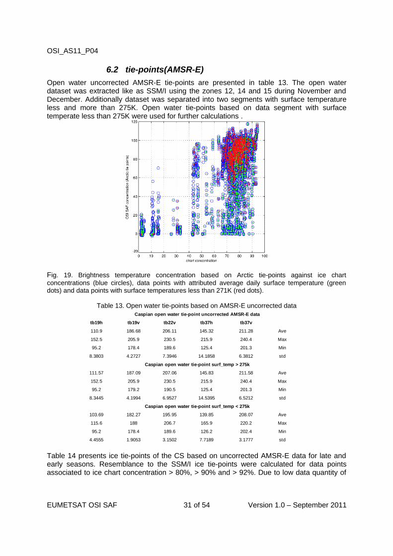
Open water uncorrected AMSR-E tie-points are presented in table 13. The open water dataset was extracted like as SSM/I using the zones 12, 14 and 15 during November and December. Additionally dataset was separated into two segments with surface temperature less and more than 275K. Open water tie-points based on data segment with surface temperate less than 275K were used for further calculations .
Fig. 19. Brightness temperature concentration based on Arctic tie-points against ice chart concentrations (blue circles), data points with attributed average daily surface temperature (green dots) and data points with surface temperatures less than 271K (red dots).
Table 13. Open water tie-points based on AMSR-E uncorrected data
Table 14 presents ice tie-points of the CS based on uncorrected AMSR-E data for late and early seasons. Resemblance to the SSM/I ice tie-points were calculated for data points associated to ice chart concentration > 80%, > 90% and > 92%. Due to low data quantity of
EUMETSAT OSI SAF 31 of 54 Version 1.0 – September 2011
Caspian open water tie-point uncorrected AMSR-E data
tb19h tb19v tb22v tb37h tb37v
110.9 186.68 206.11 145.32 211.28 Ave
152.5 205.9 230.5 215.9 240.4 Max
95.2 178.4 189.6 125.4 201.3 Min
8.3803 4.2727 7.3946 14.1858 6.3812 std
Caspian open water tie-point surf_temp > 275k
111.57 187.09 207.06 145.83 211.58 Ave
152.5 205.9 230.5 215.9 240.4 Max
95.2 179.2 190.5 125.4 201.3 Min
8.3445 4.1994 6.9527 14.5395 6.5212 std
Caspian open water tie-point surf_temp < 275k
103.69 182.27 195.95 139.85 208.07 Ave
115.6 188 206.7 165.9 220.2 Max
95.2 178.4 189.6 126.2 202.4 Min
4.4555 1.9053 3.1502 7.7189 3.1777 std
OSI_AS11_P04
data points for ice chart concentration more than 90% only tie-point for > 80% was determined for early season.
Table 14. Ice tie-points for the CS based on AMSR-E data
6.3 Sea ice concentration retrieval (AMSR-E)
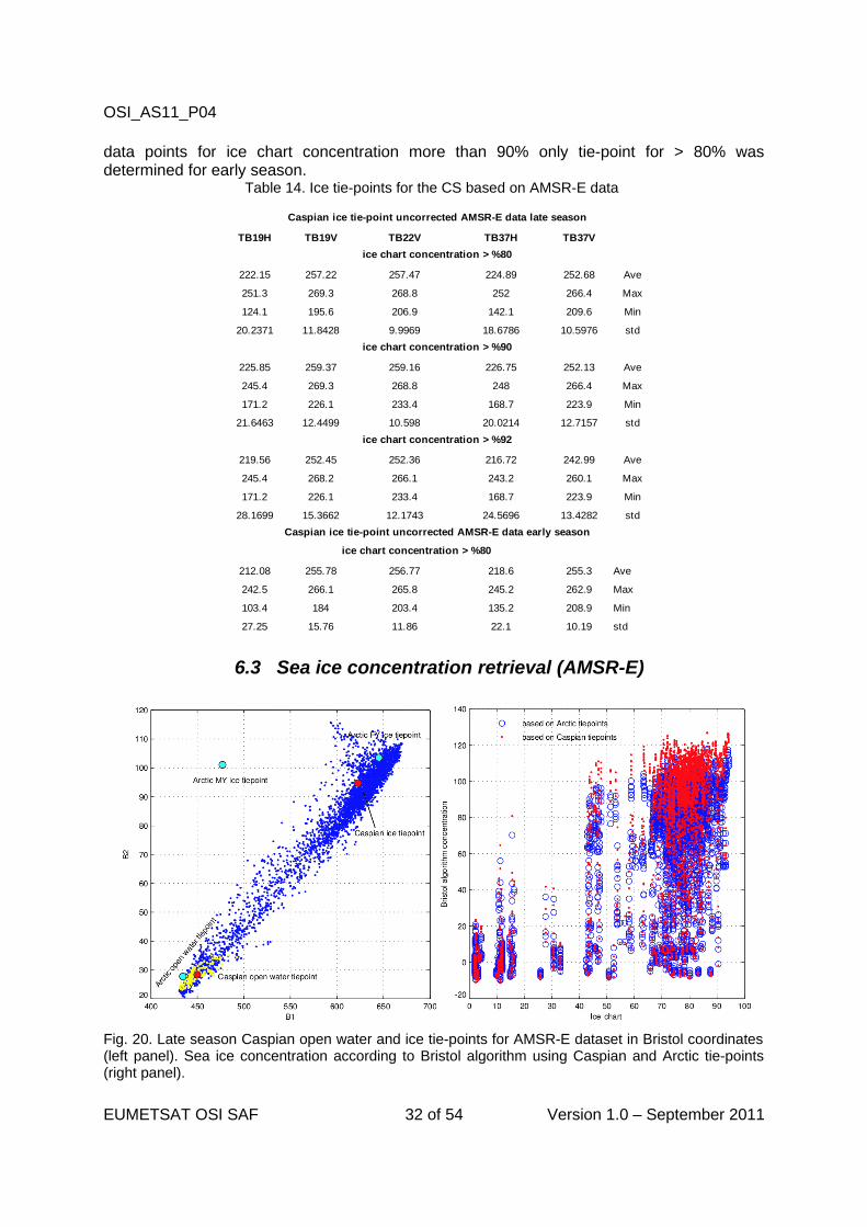
Fig. 20. Late season Caspian open water and ice tie-points for AMSR-E dataset in Bristol coordinates (left panel). Sea ice concentration according to Bristol algorithm using Caspian and Arctic tie-points (right panel).
EUMETSAT OSI SAF 32 of 54 Version 1.0 – September 2011
Caspian ice tie-point uncorrected AMSR-E data late season
TB19H TB19V TB22V TB37H TB37V
ice chart concentration > %80
222.15 257.22 257.47 224.89 252.68 Ave
251.3 269.3 268.8 252 266.4 Max
124.1 195.6 206.9 142.1 209.6 Min
20.2371 11.8428 9.9969 18.6786 10.5976 std
ice chart concentration > %90
225.85 259.37 259.16 226.75 252.13 Ave
245.4 269.3 268.8 248 266.4 Max
171.2 226.1 233.4 168.7 223.9 Min
21.6463 12.4499 10.598 20.0214 12.7157 std
ice chart concentration > %92
219.56 252.45 252.36 216.72 242.99 Ave
245.4 268.2 266.1 243.2 260.1 Max
171.2 226.1 233.4 168.7 223.9 Min
28.1699 15.3662 12.1743 24.5696 13.4282 std
Caspian ice tie-point uncorrected AMSR-E data early season
ice chart concentration > %80
212.08 255.78 256.77 218.6 255.3 Ave
242.5 266.1 265.8 245.2 262.9 Max
103.4 184 203.4 135.2 208.9 Min
27.25 15.76 11.86 22.1 10.19 std
OSI_AS11_P04
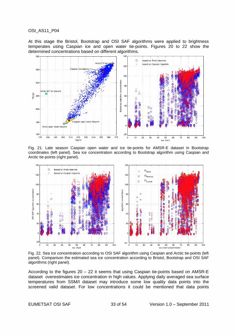
At this stage the Bristol, Bootstrap and OSI SAF algorithms were applied to brightness temperates using Caspian ice and open water tie-points. Figures 20 to 22 show the determined concentrations based on different algorithms.
Fig. 21. Late season Caspian open water and ice tie-points for AMSR-E dataset in Bootstrap coordinates (left panel). Sea ice concentration according to Bootstrap algorithm using Caspian and Arctic tie-points (right panel).
Fig. 22. Sea ice concentration according to OSI SAF algorithm using Caspian and Arctic tie-points (left panel). Comparison the estimated sea ice concentration according to Bristol, Bootstrap and OSI SAF algorithms (right panel).
According to the figures 20 – 22 it seems that using Caspian tie-points based on AMSR-E dataset overestimates ice concentration in high values. Applying daily averaged sea surface temperatures from SSM/I dataset may introduce some low quality data points into the screened valid dataset. For low concentrations it could be mentioned that data points
EUMETSAT OSI SAF 33 of 54 Version 1.0 – September 2011

OSI_AS11_P04
approximately centered around zero level and sea ice concentration improved in some degrees.
EUMETSAT OSI SAF 34 of 54 Version 1.0 – September 2011
OSI_AS11_P04
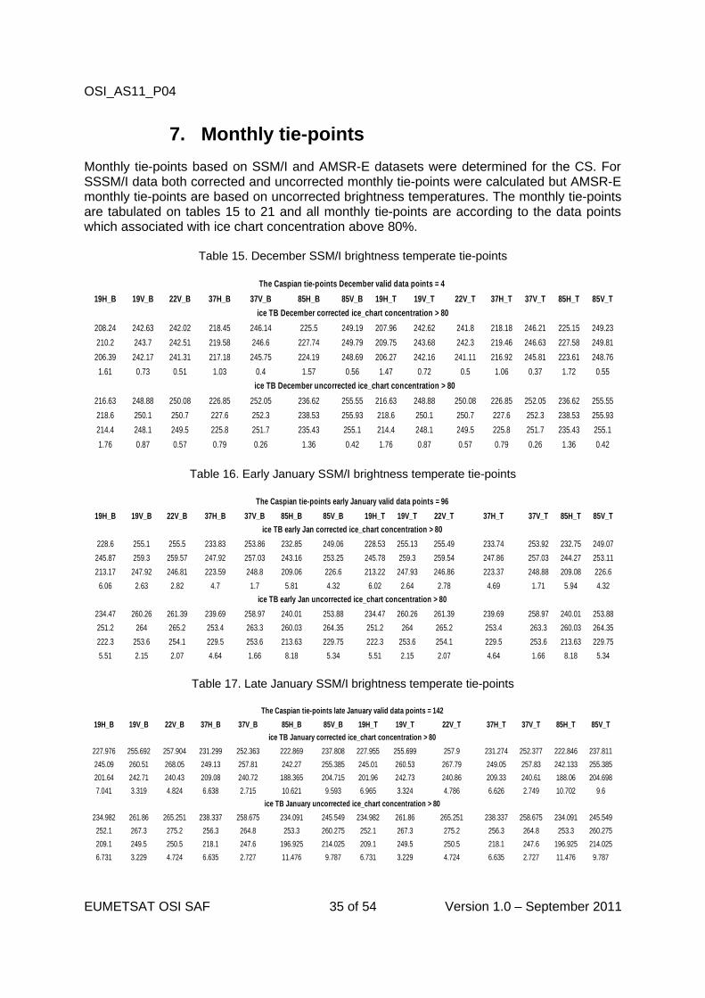
7. Monthly tie-points
Monthly tie-points based on SSM/I and AMSR-E datasets were determined for the CS. For SSSM/I data both corrected and uncorrected monthly tie-points were calculated but AMSR-E monthly tie-points are based on uncorrected brightness temperatures. The monthly tie-points are tabulated on tables 15 to 21 and all monthly tie-points are according to the data points which associated with ice chart concentration above 80%.
Table 15. December SSM/I brightness temperate tie-points
Table 16. Early January SSM/I brightness temperate tie-points
Table 17. Late January SSM/I brightness temperate tie-points
EUMETSAT OSI SAF 35 of 54 Version 1.0 – September 2011
The Caspian tie-points December valid data points = 4
19H_B 19V_B 22V_B 37H_B 37V_B 85H_B 85V_B 19H_T 19V_T 22V_T 37H_T 37V_T 85H_T 85V_T
ice TB December corrected ice_chart concentration > 80
208.24 242.63 242.02 218.45 246.14 225.5 249.19 207.96 242.62 241.8 218.18 246.21 225.15 249.23
210.2 243.7 242.51 219.58 246.6 227.74 249.79 209.75 243.68 242.3 219.46 246.63 227.58 249.81
206.39 242.17 241.31 217.18 245.75 224.19 248.69 206.27 242.16 241.11 216.92 245.81 223.61 248.76
1.61 0.73 0.51 1.03 0.4 1.57 0.56 1.47 0.72 0.5 1.06 0.37 1.72 0.55
ice TB December uncorrected ice_chart concentration > 80
216.63 248.88 250.08 226.85 252.05 236.62 255.55 216.63 248.88 250.08 226.85 252.05 236.62 255.55
218.6 250.1 250.7 227.6 252.3 238.53 255.93 218.6 250.1 250.7 227.6 252.3 238.53 255.93
214.4 248.1 249.5 225.8 251.7 235.43 255.1 214.4 248.1 249.5 225.8 251.7 235.43 255.1
1.76 0.87 0.57 0.79 0.26 1.36 0.42 1.76 0.87 0.57 0.79 0.26 1.36 0.42
The Caspian tie-points early January valid data points = 96
19H_B 19V_B 22V_B 37H_B 37V_B 85H_B 85V_B 19H_T 19V_T 22V_T 37H_T 37V_T 85H_T 85V_T
ice TB early Jan corrected ice_chart concentration > 80
228.6 255.1 255.5 233.83 253.86 232.85 249.06 228.53 255.13 255.49 233.74 253.92 232.75 249.07
245.87 259.3 259.57 247.92 257.03 243.16 253.25 245.78 259.3 259.54 247.86 257.03 244.27 253.11
213.17 247.92 246.81 223.59 248.8 209.06 226.6 213.22 247.93 246.86 223.37 248.88 209.08 226.6
6.06 2.63 2.82 4.7 1.7 5.81 4.32 6.02 2.64 2.78 4.69 1.71 5.94 4.32
ice TB early Jan uncorrected ice_chart concentration > 80
234.47 260.26 261.39 239.69 258.97 240.01 253.88 234.47 260.26 261.39 239.69 258.97 240.01 253.88
251.2 264 265.2 253.4 263.3 260.03 264.35 251.2 264 265.2 253.4 263.3 260.03 264.35
222.3 253.6 254.1 229.5 253.6 213.63 229.75 222.3 253.6 254.1 229.5 253.6 213.63 229.75
5.51 2.15 2.07 4.64 1.66 8.18 5.34 5.51 2.15 2.07 4.64 1.66 8.18 5.34
The Caspian tie-points late January valid data points = 142
19H_B 19V_B 22V_B 37H_B 37V_B 85H_B 85V_B 19H_T 19V_T 22V_T 37H_T 37V_T 85H_T 85V_T
ice TB January corrected ice_chart concentration > 80
227.976 255.692 257.904 231.299 252.363 222.869 237.808 227.955 255.699 257.9 231.274 252.377 222.846 237.811
245.09 260.51 268.05 249.13 257.81 242.27 255.385 245.01 260.53 267.79 249.05 257.83 242.133 255.385
201.64 242.71 240.43 209.08 240.72 188.365 204.715 201.96 242.73 240.86 209.33 240.61 188.06 204.698
7.041 3.319 4.824 6.638 2.715 10.621 9.593 6.965 3.324 4.786 6.626 2.749 10.702 9.6
ice TB January uncorrected ice_chart concentration > 80
234.982 261.86 265.251 238.337 258.675 234.091 245.549 234.982 261.86 265.251 238.337 258.675 234.091 245.549
252.1 267.3 275.2 256.3 264.8 253.3 260.275 252.1 267.3 275.2 256.3 264.8 253.3 260.275
209.1 249.5 250.5 218.1 247.6 196.925 214.025 209.1 249.5 250.5 218.1 247.6 196.925 214.025
6.731 3.229 4.724 6.635 2.727 11.476 9.787 6.731 3.229 4.724 6.635 2.727 11.476 9.787
OSI_AS11_P04
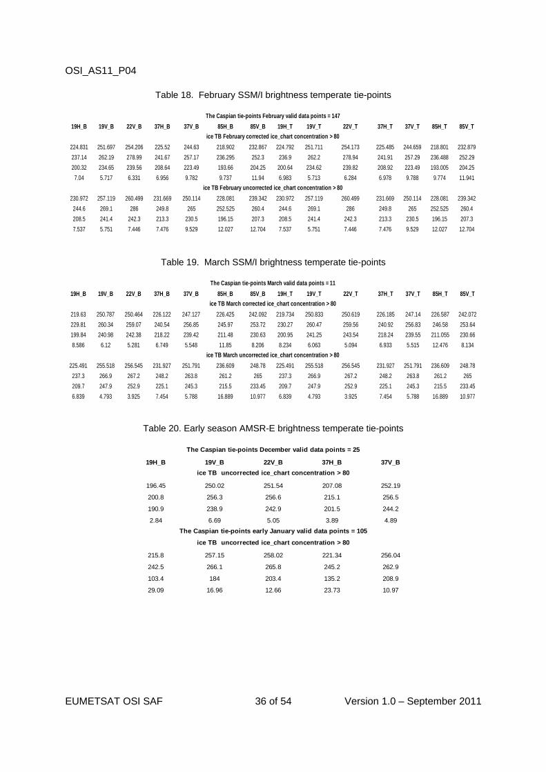
Table 18. February SSM/I brightness temperate tie-points
Table 19. March SSM/I brightness temperate tie-points
Table 20. Early season AMSR-E brightness temperate tie-points
EUMETSAT OSI SAF 36 of 54 Version 1.0 – September 2011
The Caspian tie-points February valid data points = 147
19H_B 19V_B 22V_B 37H_B 37V_B 85H_B 85V_B 19H_T 19V_T 22V_T 37H_T 37V_T 85H_T 85V_T
ice TB February corrected ice_chart concentration > 80
224.831 251.697 254.206 225.52 244.63 218.902 232.867 224.792 251.711 254.173 225.485 244.659 218.801 232.879
237.14 262.19 278.99 241.67 257.17 236.295 252.3 236.9 262.2 278.94 241.91 257.29 236.488 252.29
200.32 234.65 239.56 208.64 223.49 193.66 204.25 200.64 234.62 239.82 208.92 223.49 193.005 204.25
7.04 5.717 6.331 6.956 9.782 9.737 11.94 6.983 5.713 6.284 6.978 9.788 9.774 11.941
ice TB February uncorrected ice_chart concentration > 80
230.972 257.119 260.499 231.669 250.114 228.081 239.342 230.972 257.119 260.499 231.669 250.114 228.081 239.342
244.6 269.1 286 249.8 265 252.525 260.4 244.6 269.1 286 249.8 265 252.525 260.4
208.5 241.4 242.3 213.3 230.5 196.15 207.3 208.5 241.4 242.3 213.3 230.5 196.15 207.3
7.537 5.751 7.446 7.476 9.529 12.027 12.704 7.537 5.751 7.446 7.476 9.529 12.027 12.704
The Caspian tie-points March valid data points = 11
19H_B 19V_B 22V_B 37H_B 37V_B 85H_B 85V_B 19H_T 19V_T 22V_T 37H_T 37V_T 85H_T 85V_T
ice TB March corrected ice_chart concentration > 80
219.63 250.787 250.464 226.122 247.127 226.425 242.092 219.734 250.833 250.619 226.185 247.14 226.587 242.072
229.81 260.34 259.07 240.54 256.85 245.97 253.72 230.27 260.47 259.56 240.92 256.83 246.58 253.64
199.84 240.98 242.38 218.22 239.42 211.48 230.63 200.95 241.25 243.54 218.24 239.55 211.055 230.66
8.586 6.12 5.281 6.749 5.548 11.85 8.206 8.234 6.063 5.094 6.933 5.515 12.476 8.134
ice TB March uncorrected ice_chart concentration > 80
225.491 255.518 256.545 231.927 251.791 236.609 248.78 225.491 255.518 256.545 231.927 251.791 236.609 248.78
237.3 266.9 267.2 248.2 263.8 261.2 265 237.3 266.9 267.2 248.2 263.8 261.2 265
209.7 247.9 252.9 225.1 245.3 215.5 233.45 209.7 247.9 252.9 225.1 245.3 215.5 233.45
6.839 4.793 3.925 7.454 5.788 16.889 10.977 6.839 4.793 3.925 7.454 5.788 16.889 10.977
The Caspian tie-points December valid data points = 25
19H_B 19V_B 22V_B 37H_B 37V_B
ice TB uncorrected ice_chart concentration > 80
196.45 250.02 251.54 207.08 252.19
200.8 256.3 256.6 215.1 256.5
190.9 238.9 242.9 201.5 244.2
2.84 6.69 5.05 3.89 4.89
The Caspian tie-points early January valid data points = 105
ice TB uncorrected ice_chart concentration > 80
215.8 257.15 258.02 221.34 256.04
242.5 266.1 265.8 245.2 262.9
103.4 184 203.4 135.2 208.9
29.09 16.96 12.66 23.73 10.97
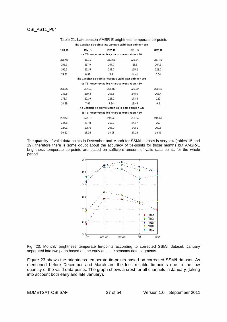
OSI_AS11_P04
Table 21. Late season AMSR-E brightness temperate tie-points
The quantity of valid data points in December and March for SSM/I dataset is very low (tables 15 and 19), therefore there is some doubt about the accuracy of tie-points for those months but AMSR-E brightness temperate tie-points are based on sufficient amount of valid data points for the whole period.
Fig. 23. Monthly brightness temperate tie-points according to corrected SSM/I dataset. January separated into two parts based on the early and late seasons data segments.
Figure 23 shows the brightness temperate tie-points based on corrected SSM/I dataset. As mentioned before December and March are the less reliable tie-points due to the low quantity of the valid data points. The graph shows a crest for all channels in January (taking into account both early and late January).
EUMETSAT OSI SAF 37 of 54 Version 1.0 – September 2011
The Caspian tie-points late January valid data points = 295
19H_B 19V_B 22V_B 37H_B 37V_B
ice TB uncorrected ice_chart concentration > 80
225.08 261.1 261.55 228.74 257.42
251.3 267.9 267.7 252 264.3
165.3 221.5 231.7 165.2 223.2
15.21 6.99 5.4 14.41 5.54
The Caspian tie-points February valid data points = 203
ice TB uncorrected ice_chart concentration > 80
226.25 257.81 256.88 226.99 250.48
245.8 269.3 268.8 248.5 266.4
173.7 221.9 228.2 173.3 222
14.29 7.97 7.34 13.45 9.9
The Caspian tie-points March valid data points = 135
ice TB uncorrected ice_chart concentration > 80
209.59 247.87 249.45 213.34 245.67
244.8 267.8 267.3 244.7 266
124.1 195.6 206.9 142.1 209.6
30.22 18.35 14.98 27.26 14.43
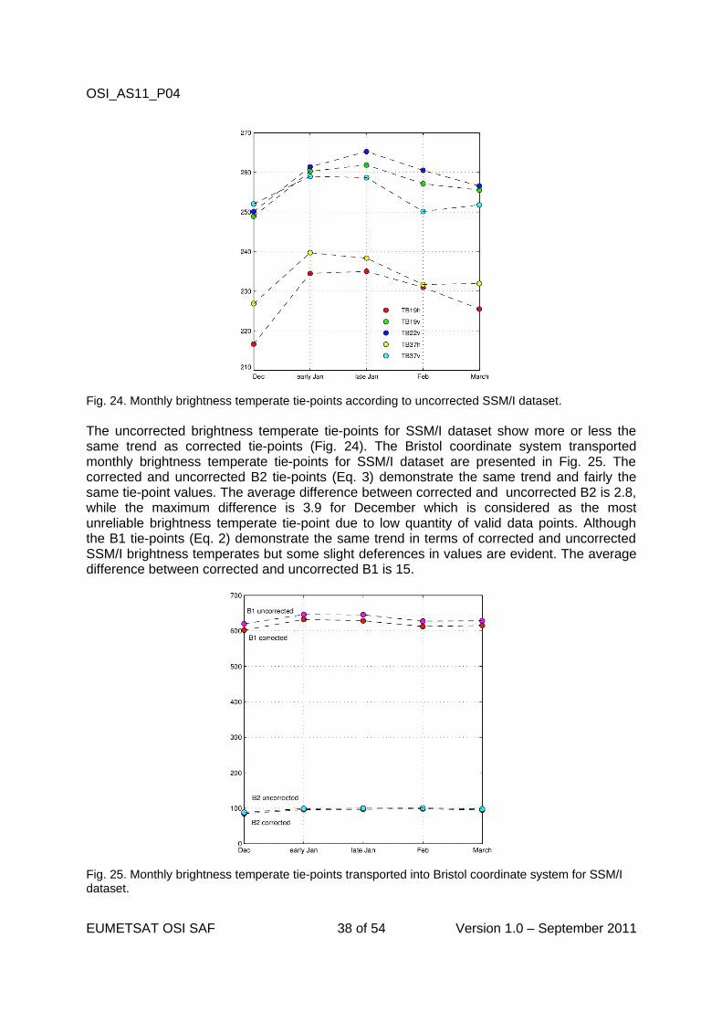
OSI_AS11_P04
Fig. 24. Monthly brightness temperate tie-points according to uncorrected SSM/I dataset.
The uncorrected brightness temperate tie-points for SSM/I dataset show more or less the same trend as corrected tie-points (Fig. 24). The Bristol coordinate system transported monthly brightness temperate tie-points for SSM/I dataset are presented in Fig. 25. The corrected and uncorrected B2 tie-points (Eq. 3) demonstrate the same trend and fairly the same tie-point values. The average difference between corrected and uncorrected B2 is 2.8, while the maximum difference is 3.9 for December which is considered as the most unreliable brightness temperate tie-point due to low quantity of valid data points. Although the B1 tie-points (Eq. 2) demonstrate the same trend in terms of corrected and uncorrected SSM/I brightness temperates but some slight deferences in values are evident. The average difference between corrected and uncorrected B1 is 15.
Fig. 25. Monthly brightness temperate tie-points transported into Bristol coordinate system for SSM/I dataset.
EUMETSAT OSI SAF 38 of 54 Version 1.0 – September 2011
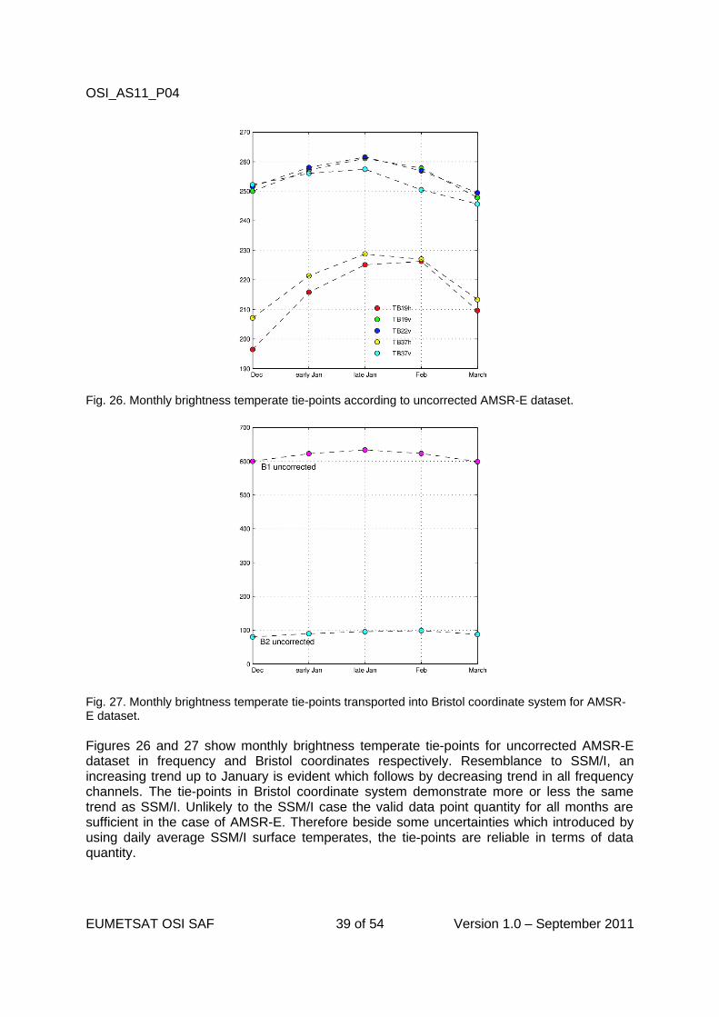
OSI_AS11_P04
Fig. 26. Monthly brightness temperate tie-points according to uncorrected AMSR-E dataset.
Fig. 27. Monthly brightness temperate tie-points transported into Bristol coordinate system for AMSR-E dataset.
Figures 26 and 27 show monthly brightness temperate tie-points for uncorrected AMSR-E dataset in frequency and Bristol coordinates respectively. Resemblance to SSM/I, an increasing trend up to January is evident which follows by decreasing trend in all frequency channels. The tie-points in Bristol coordinate system demonstrate more or less the same trend as SSM/I. Unlikely to the SSM/I case the valid data point quantity for all months are sufficient in the case of AMSR-E. Therefore beside some uncertainties which introduced by using daily average SSM/I surface temperates, the tie-points are reliable in terms of data quantity.
EUMETSAT OSI SAF 39 of 54 Version 1.0 – September 2011
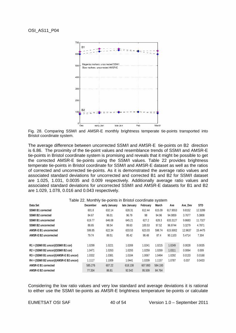
OSI_AS11_P04
Fig. 28. Comparing SSM/I and AMSR-E monthly brightness temperate tie-points transported into Bristol coordinate system.
The average difference between uncorrected SSM/I and AMSR-E tie-points on B2 direction is 6.86. The proximity of the tie-point values and resemblance trends of SSM/I and AMSR-E tie-points in Bristol coordinate system is promising and reveals that it might be possible to get the corrected AMSR-E tie-points using the SSM/I values. Table 22 provides brightness temperate tie-points in Bristol coordinate for SSM/I and AMSR-E dataset as well as the ratios of corrected and uncorrected tie-points. As it is demonstrated the average ratio values and associated standard deviations for uncorrected and corrected B1 and B2 for SSM/I dataset are 1.025, 1.031, 0.0035 and 0.009 respectively. Additionally average ratio values and associated standard deviations for uncorrected SSM/I and AMSR-E datasets for B1 and B2 are 1.029, 1.078, 0.016 and 0.043 respectively.
Table 22. Monthly tie-points in Bristol coordinate system
Considering the low ratio values and very low standard and average deviations it is rational to either use the SSM/I tie-points as AMSR-E brightness temperature tie-points or calculate
EUMETSAT OSI SAF 40 of 54 Version 1.0 – September 2011
Data Set December early January late January February March Ave Ave_Dev STD
SSM/I B1 corrected 601.8 632.14 628.31 612.44 615.09 617.9553 9.8152 12.3289
SSM/I B2 corrected 84.67 96.01 96.79 98 94.96 94.0859 3.7677 5.3808
SSM/I B1 uncorrected 619.77 646.08 645.21 627.2 628.3 633.3127 9.8683 11.7327
SSM/I B2 uncorrected 88.65 98.54 99.63 100.53 97.52 96.9744 3.3279 4.7871
AMSR-E B1 uncorrected 599.85 622.34 633.53 623.03 598.74 615.5002 12.9637 15.4475
AMSR-E B2 uncorrected 79.74 89.51 95.42 98.48 87.4 90.1103 5.4714 7.304
1.0299 1.0221 1.0269 1.0241 1.0215 1.0249 0.0028 0.0035
1.0471 1.0263 1.0293 1.0259 1.0269 1.0311 0.0064 0.009
1.0332 1.0381 1.0184 1.0067 1.0494 1.0292 0.0133 0.0168
1.1117 1.1009 1.0441 1.0209 1.1157 1.0787 0.037 0.0433
AMSR-E B1 corrected 585.276 607.22 618.138 607.893 584.193
AMSR-E B2 corrected 77.334 86.81 92.542 95.509 84.764
R1 = (SSM/I B1 uncor)/(SSM/I B1 cor)
R2 = (SSM/I B2 uncor)/(SSM/I B2 cor)
R3 = (SSM/I B1 uncor)/(AMSR-E B1 uncor)
R4 = (SSM/I B2 uncor)/(AMSR-E B2 uncor)
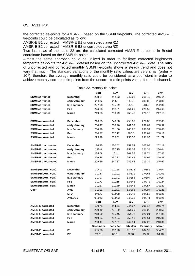
OSI_AS11_P04
the corrected tie-points for AMSR-E based on the SSM/I tie-points. The corrected AMSR-E tie-points could be calculated as follow:AMSR-E B1 corrected = AMSR-E B1 uncorrected / ave(R1)AMSR-E B2 corrected = AMSR-E B2 uncorrected / ave(R2)Two last rows of the table 22 are the calculated corrected AMSR-E tie-points in Bristol coordinate based on the SSM/I tie-points. Almost the same approach could be utilized in order to facilitate corrected brightness temperate tie-points for AMSR-E dataset based on the uncorrected AMSR-E data. The ratio of uncorrected and corrected monthly SSM/I tie-points shows a steady trend and does not vary that much. The standard variations of the monthly ratio values are very small (order ~ 10-3), therefore the average monthly ratio could be considered as a coefficient in order to achieve monthly corrected tie-points from the uncorrected tie-points values for each channel.
Table 22. Monthly tie-points
EUMETSAT OSI SAF 41 of 54 Version 1.0 – September 2011
19H 19V 22V 37H 37V
SSM/I corrected December 208.24 242.63 242.02 218.45 246.14
SSM/I corrected early January 228.6 255.1 255.5 233.83 253.86
SSM/I corrected late January 227.98 255.69 257.9 231.3 252.36
SSM/I corrected Feb 224.83 251.7 254.21 225.52 244.63
SSM/I corrected March 219.63 250.79 250.46 226.12 247.13
SSM/I uncorrected December 216.63 248.88 250.08 226.85 252.05
SSM/I uncorrected early January 234.47 260.26 261.39 239.69 258.97
SSM/I uncorrected late January 234.98 261.86 265.25 238.34 258.68
SSM/I uncorrected Feb 230.97 257.12 260.5 231.67 250.11
SSM/I uncorrected March 225.49 255.52 256.55 231.93 251.79
AMSR-E uncorrected December 196.45 250.02 251.54 207.08 252.19
AMSR-E uncorrected early January 215.8 257.15 258.02 221.34 256.04
AMSR-E uncorrected late January 225.08 261.1 261.55 228.74 257.42
AMSR-E uncorrected Feb 226.25 257.81 256.88 226.99 250.48
AMSR-E uncorrected March 209.59 247.87 249.45 213.34 245.67
December 1.0403 1.0258 1.0333 1.0385 1.024
early January 1.0257 1.0202 1.0231 1.0251 1.0201
late January 1.0307 1.0241 1.0285 1.0304 1.025
Feb 1.0273 1.0215 1.0248 1.0273 1.0224
March 1.0267 1.0189 1.0243 1.0257 1.0189
AVE 1.0301 1.0221 1.0268 1.0294 1.0221
STD 0.006 0.0028 0.0042 0.0055 0.0026
AVEDEV 0.0043 0.0023 0.0033 0.0041 0.0021
19H 19V 22V 37H 37V
AMSR-E corrected December 190.71 244.61 244.97 201.17 246.74
AMSR-E corrected early January 209.49 251.59 251.29 215.02 250.50
AMSR-E corrected late January 218.50 255.45 254.72 222.21 251.85
AMSR-E corrected Feb 219.64 252.24 250.18 220.51 245.06
AMSR-E corrected March 203.47 242.51 242.94 207.25 240.36
December early Jan late Jan February March
AMSR-E corrected B1 585.38 607.28 618.17 607.92 584.25
AMSR-E corrected B2 77.31 86.81 92.57 95.57 84.78
SSM/I (uncorr / corr)
SSM/I (uncorr / corr)
SSM/I (uncorr / corr)
SSM/I (uncorr / corr)
SSM/I (uncorr / corr)
Coef.
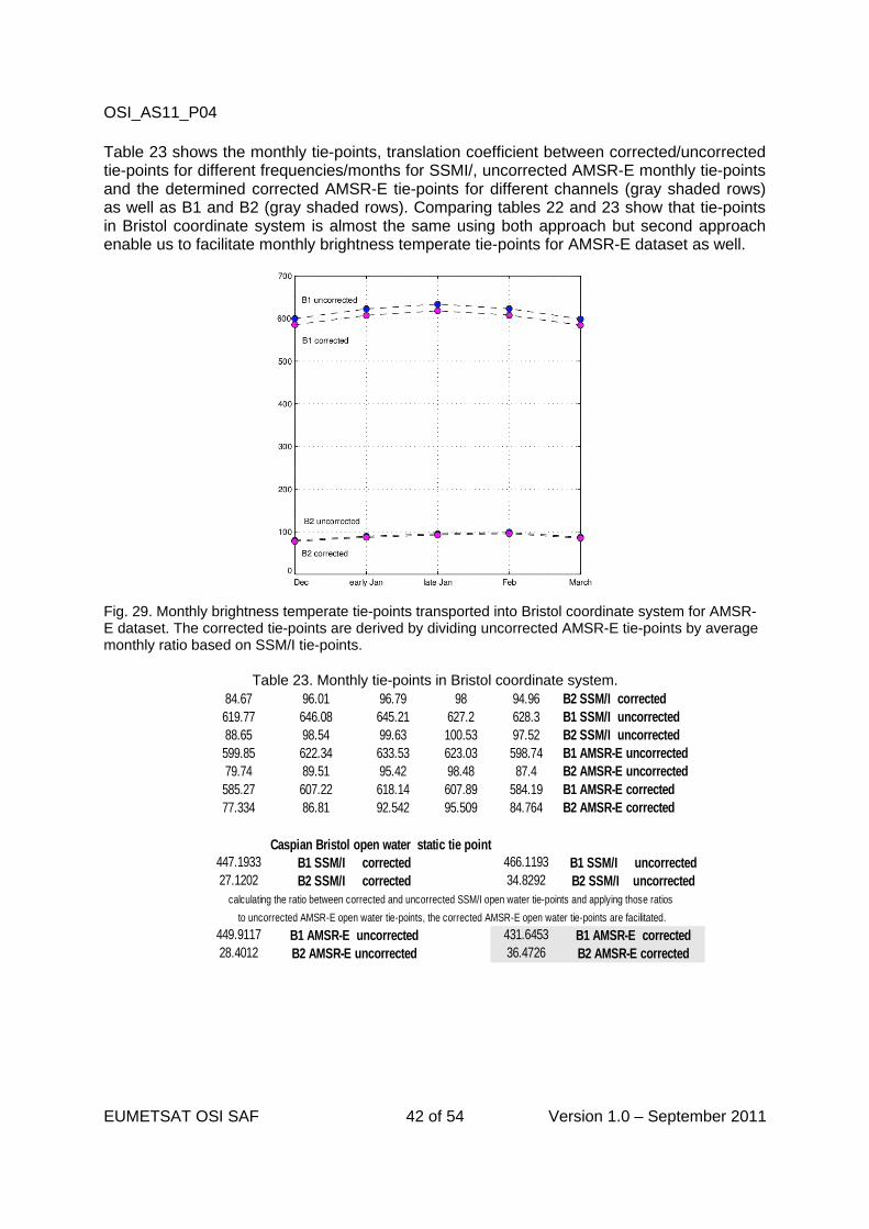
OSI_AS11_P04
Table 23 shows the monthly tie-points, translation coefficient between corrected/uncorrected tie-points for different frequencies/months for SSMI/, uncorrected AMSR-E monthly tie-points and the determined corrected AMSR-E tie-points for different channels (gray shaded rows) as well as B1 and B2 (gray shaded rows). Comparing tables 22 and 23 show that tie-points in Bristol coordinate system is almost the same using both approach but second approach enable us to facilitate monthly brightness temperate tie-points for AMSR-E dataset as well.
Fig. 29. Monthly brightness temperate tie-points transported into Bristol coordinate system for AMSR-E dataset. The corrected tie-points are derived by dividing uncorrected AMSR-E tie-points by average monthly ratio based on SSM/I tie-points.
Table 23. Monthly tie-points in Bristol coordinate system.
EUMETSAT OSI SAF 42 of 54 Version 1.0 – September 2011
84.67 96.01 96.79 98 94.96 B2 SSM/I corrected619.77 646.08 645.21 627.2 628.3 B1 SSM/I uncorrected88.65 98.54 99.63 100.53 97.52 B2 SSM/I uncorrected599.85 622.34 633.53 623.03 598.74 B1 AMSR-E uncorrected79.74 89.51 95.42 98.48 87.4 B2 AMSR-E uncorrected585.27 607.22 618.14 607.89 584.19 B1 AMSR-E corrected77.334 86.81 92.542 95.509 84.764 B2 AMSR-E corrected
Caspian Bristol open water static tie point447.1933 B1 SSM/I corrected 466.1193 B1 SSM/I uncorrected27.1202 B2 SSM/I corrected 34.8292 B2 SSM/I uncorrected
calculating the ratio between corrected and uncorrected SSM/I open water tie-points and applying those ratios
to uncorrected AMSR-E open water tie-points, the corrected AMSR-E open water tie-points are facilitated.
449.9117 B1 AMSR-E uncorrected 431.6453 B1 AMSR-E corrected28.4012 B2 AMSR-E uncorrected 36.4726 B2 AMSR-E corrected
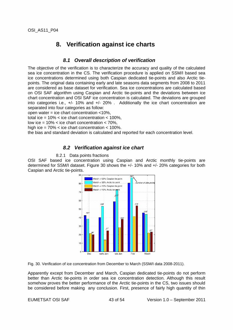
OSI_AS11_P04
8. Verification against ice charts
8.1 Overall description of verification
The objective of the verification is to characterize the accuracy and quality of the calculated sea ice concentration in the CS. The verification procedure is applied on SSM/I based sea ice concentrations determined using both Caspian dedicated tie-points and also Arctic tie-points. The original data containing early and late seasons data segments from 2008 to 2011 are considered as base dataset for verification. Sea ice concentrations are calculated based on OSI SAF algorithm using Caspian and Arctic tie-points and the deviations between ice chart concentration and OSI SAF ice concentration is calculated. The deviations are grouped into categories i.e., +/- 10% and +/- 20% . Additionally the ice chart concentration are separated into four categories as follow:open water = ice chart concentration <10%,total ice = 10% < ice chart concentration < 100%,low ice = 10% < ice chart concentration < 70%,high ice = 70% < ice chart concentration < 100%.the bias and standard deviation is calculated and reported for each concentration level.
8.2 Verification against ice chart
8.2.1 Data points fractionsOSI SAF based ice concentration using Caspian and Arctic monthly tie-points are determined for SSM/I dataset. Figure 30 shows the +/- 10% and +/- 20% categories for both Caspian and Arctic tie-points.
Fig. 30. Verification of ice concentration from December to March (SSM/I data 2008-2011).
Apparently except from December and March, Caspian dedicated tie-points do not perform better than Arctic tie-points in order sea ice concentration detection. Although this result somehow proves the better performance of the Arctic tie-points in the CS, two issues should be considered before making any conclusion. First, presence of fairly high quantity of thin
EUMETSAT OSI SAF 43 of 54 Version 1.0 – September 2011
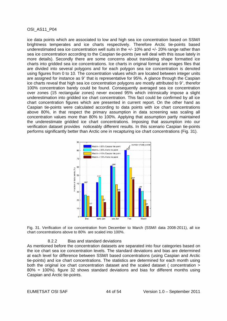
OSI_AS11_P04
ice data points which are associated to low and high sea ice concentration based on SSM/I brightness temperates and ice charts respectively. Therefore Arctic tie-points based underestimated sea ice concentration well suits in the +/- 10% and +/- 20% range rather than sea ice concentration according to the Caspian tie-points (we will deal with this issue lately in more details). Secondly there are some concerns about translating shape formatted ice charts into gridded sea ice concentrations. Ice charts in original format are images files that are divided into several polygons and for each polygon sea ice concentration is denoted using figures from 0 to 10. The concentration values which are located between integer units are assigned for instance as 9+ that is representative for 95%. A glance through the Caspian ice charts reveal that high sea ice concentration polygons are mostly attributed to 9+, therefor 100% concentration barely could be found. Consequently averaged sea ice concentration over zones (15 rectangular zones) never exceed 95% which intrinsically impose a slight underestimation into gridded ice chart concentration. This fact could be confirmed by all ice chart concentration figures which are presented in current report. On the other hand as Caspian tie-points were calculated according to data points with ice chart concentrations above 80%, in that respect the primary assumption in data screening was scaling all concentration values more than 80% to 100%. Applying that assumption partly maintained the underestimate gridded ice chart concentrations. Imposing that assumption into our verification dataset provides noticeably different results. In this scenario Caspian tie-points performs significantly better than Arctic one in recapturing ice chart concentrations (Fig. 31).
Fig. 31. Verification of ice concentration from December to March (SSM/I data 2008-2011), all ice chart concentrations above to 80% are scaled into 100%.
8.2.2 Bias and standard deviationsAs mentioned before the concentration datasets are separated into four categories based on the ice chart sea ice concentration levels. The standard deviations and bias are determined at each level for difference between SSM/I based concentrations (using Caspian and Arctic tie-points) and ice chart concentrations. The statistics are determined for each month using both the original ice chart concentration dataset and the scaled dataset ( concentration > 80% = 100%). figure 32 shows standard deviations and bias for different months using Caspian and Arctic tie-points.
EUMETSAT OSI SAF 44 of 54 Version 1.0 – September 2011
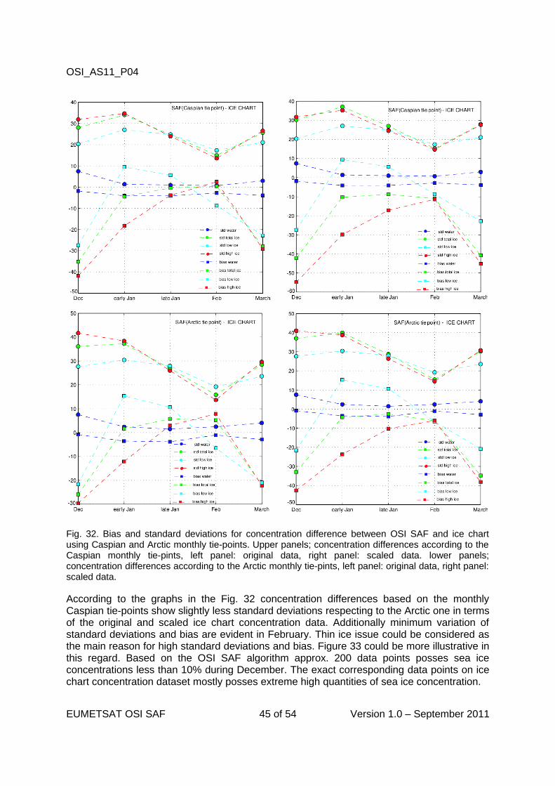
OSI_AS11_P04
Fig. 32. Bias and standard deviations for concentration difference between OSI SAF and ice chart using Caspian and Arctic monthly tie-points. Upper panels; concentration differences according to the Caspian monthly tie-pints, left panel: original data, right panel: scaled data. lower panels; concentration differences according to the Arctic monthly tie-pints, left panel: original data, right panel: scaled data.
According to the graphs in the Fig. 32 concentration differences based on the monthly Caspian tie-points show slightly less standard deviations respecting to the Arctic one in terms of the original and scaled ice chart concentration data. Additionally minimum variation of standard deviations and bias are evident in February. Thin ice issue could be considered as the main reason for high standard deviations and bias. Figure 33 could be more illustrative in this regard. Based on the OSI SAF algorithm approx. 200 data points posses sea ice concentrations less than 10% during December. The exact corresponding data points on ice chart concentration dataset mostly posses extreme high quantities of sea ice concentration.
EUMETSAT OSI SAF 45 of 54 Version 1.0 – September 2011
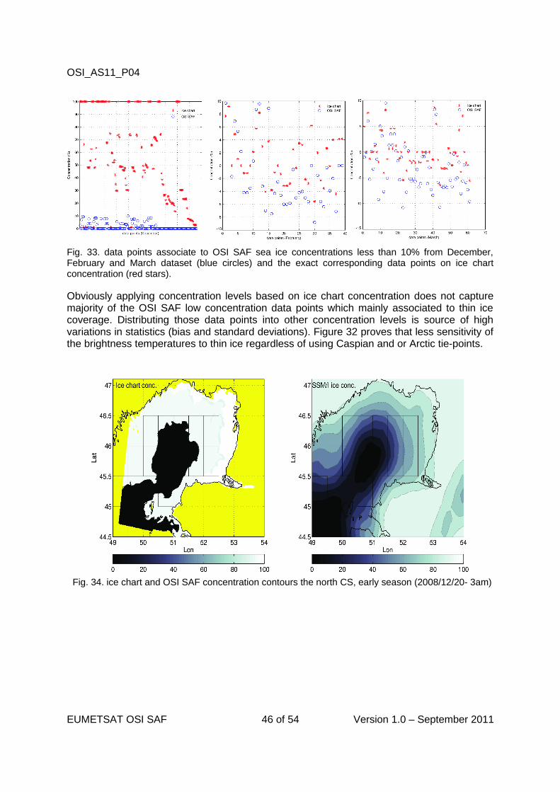
OSI_AS11_P04
Fig. 33. data points associate to OSI SAF sea ice concentrations less than 10% from December, February and March dataset (blue circles) and the exact corresponding data points on ice chart concentration (red stars).
Obviously applying concentration levels based on ice chart concentration does not capture majority of the OSI SAF low concentration data points which mainly associated to thin ice coverage. Distributing those data points into other concentration levels is source of high variations in statistics (bias and standard deviations). Figure 32 proves that less sensitivity of the brightness temperatures to thin ice regardless of using Caspian and or Arctic tie-points.
Fig. 34. ice chart and OSI SAF concentration contours the north CS, early season (2008/12/20- 3am)
EUMETSAT OSI SAF 46 of 54 Version 1.0 – September 2011
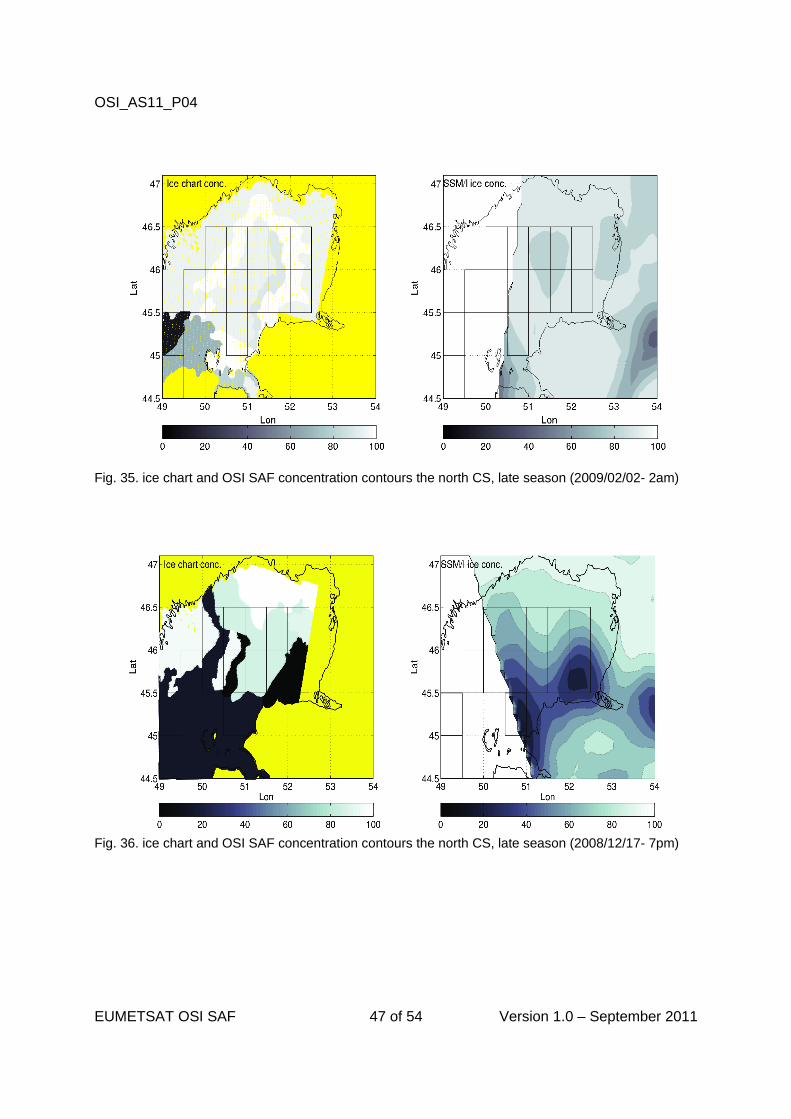
OSI_AS11_P04
Fig. 35. ice chart and OSI SAF concentration contours the north CS, late season (2009/02/02- 2am)
Fig. 36. ice chart and OSI SAF concentration contours the north CS, late season (2008/12/17- 7pm)
EUMETSAT OSI SAF 47 of 54 Version 1.0 – September 2011
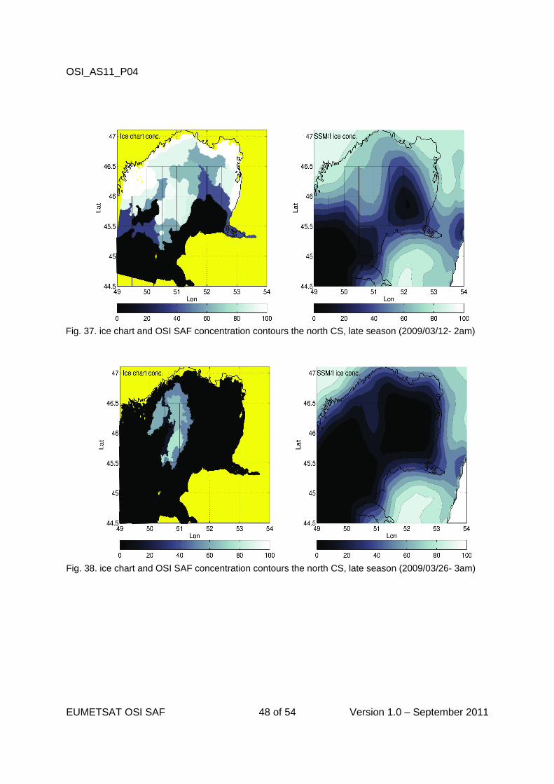
OSI_AS11_P04
Fig. 37. ice chart and OSI SAF concentration contours the north CS, late season (2009/03/12- 2am)
Fig. 38. ice chart and OSI SAF concentration contours the north CS, late season (2009/03/26- 3am)
EUMETSAT OSI SAF 48 of 54 Version 1.0 – September 2011
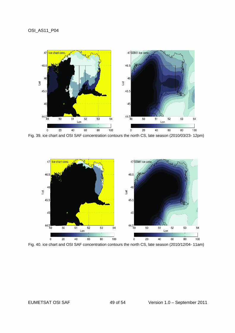
OSI_AS11_P04
Fig. 39. ice chart and OSI SAF concentration contours the north CS, late season (2010/03/23- 12pm)
Fig. 40. ice chart and OSI SAF concentration contours the north CS, late season (2010/12/04- 11am)
EUMETSAT OSI SAF 49 of 54 Version 1.0 – September 2011
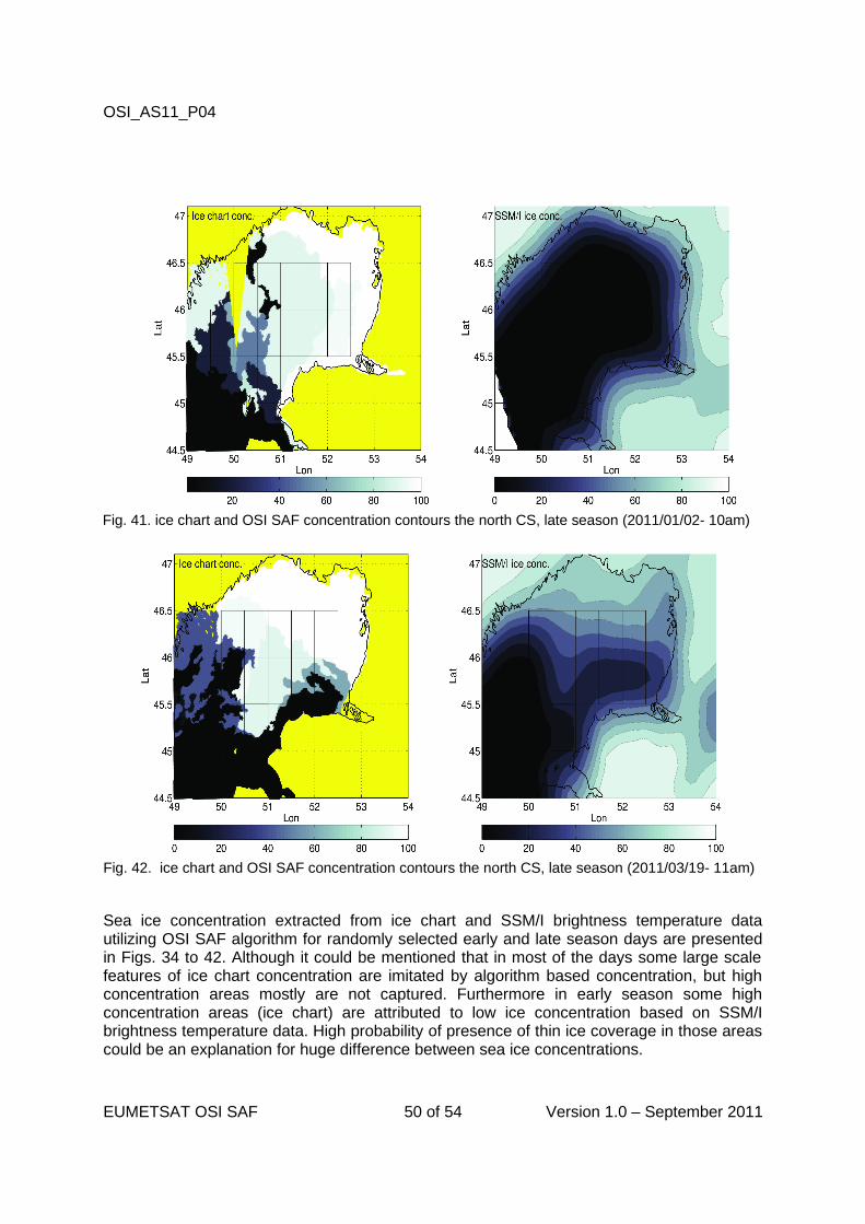
OSI_AS11_P04
Fig. 41. ice chart and OSI SAF concentration contours the north CS, late season (2011/01/02- 10am)
Fig. 42. ice chart and OSI SAF concentration contours the north CS, late season (2011/03/19- 11am)
Sea ice concentration extracted from ice chart and SSM/I brightness temperature data utilizing OSI SAF algorithm for randomly selected early and late season days are presented in Figs. 34 to 42. Although it could be mentioned that in most of the days some large scale features of ice chart concentration are imitated by algorithm based concentration, but high concentration areas mostly are not captured. Furthermore in early season some high concentration areas (ice chart) are attributed to low ice concentration based on SSM/I brightness temperature data. High probability of presence of thin ice coverage in those areas could be an explanation for huge difference between sea ice concentrations.
EUMETSAT OSI SAF 50 of 54 Version 1.0 – September 2011
OSI_AS11_P04
9. Concluding remarks
The investigation has demonstrated that the Caspian Sea ice can be estimated from satellite microwave radiometer measurements using standard ice concentration algorithms as used in the Arctic and Antarctic. However, some biases should be expected if using Arctic or Antarctic tie points.The study therefore investigated and derived special tie-points for the Caspian Sea, and developed a method for determining such regional tie-points that can subsequently be applied to other regions such as the Baltic, the Great Lakes or the Hudson Bay where ice signatures also deviate somewhat from typical signatures in the Arctic or Antarctic.Investigations using a combination of sea ice charts from the Danish Meteorological Institute and SSMI and AMSR satellite microwave radiometer data showed that even when using dedicated tie-points, some biases in ice concentrations during the early season when the ice is very thin cannot be avoided. The concentration of thin ice will be somewhat underestimated and users of products should be made aware of this fact.The tie-points derived in this project are ready for implementation, and the OSISAF ice concentration coverage can be extended to include the Caspian Sea when the new coverage area is defined.
EUMETSAT OSI SAF 51 of 54 Version 1.0 – September 2011

OSI_AS11_P04
10. Acknowledgement
We gratefully acknowledge AGIP-oil for allowing the use of a set of their DMI ice-charts from the Caspian Sea for these investigations.
EUMETSAT OSI SAF 52 of 54 Version 1.0 – September 2011
OSI_AS11_P04
11. References
Andersen, S., R. Tonboe, S. Kern, H. Schyberg (2006) Improved retrieval of sea ice total concentration from spaceborne passive microwave observations using numerical weather model fields: An intercomparision of nine algorithms. Remote Sensing of Environment, 104, 374-392.
Breivik, L.-A., S. Eastwood, Ø. Godøy, H. Schyberg, S. Andersen, R.T. Tonboe (2001) Sea Ice Products for EUMETSAT Satellite Application Facility. Canadian Journal of Remote Sensing, Volume 27, No. 5.
Comiso, J.C., (1986) Characteristics of Artic winter sea ice from satellite multispectral microwave observations. Journal of Geo- physical Research 91, 975 – 994.
Comiso, J.C., D.J. Cavalieri, C.L. Parkinson, P. Gloersen (1997). Passive microwave algorithms for sea ice concentration: A comparison of two techniques. Remote Sensing of Environment 60, 357-384.
Eastwood, S. (2011). OSI-SAF Sea Ice Product Manual, v3.7, 35 pages.
Eastwood, S. K.R. Larsen, T. Lavergne, R. Tonbone (2011). OSI-SAF Global Sea Ice Concentration Reprocessing. Product User Manual, v1.2, 31 pages. Foerhlich, K., A. K. Rozanski , P. Povinec , B. Oregioni , J. Gastaud (1999) Isotope studies in the Caspian Sea . The Science of the Total Environment, 237, 238, 419-427.
Ghaffari, P., V. Chegini (2010) Acoustic Doppler Current Profiler observations in the southern Caspian Sea. Ocean Sci., 6, 737-748.
Ghaffari, P., H.A. Lahijani, J. Azizpour (2010) Snapshot observation of the physical structure and stratification in deep-water of the south Caspian Sea (western part). Ocean Sci., 6, 877-885.
Kouraev , A.V., F. Papa , N.M. Mognard , P. I. Buharizin , A. Cazenave , J. F. Cretaux , J. Dozortseva , F. Remy (2004) Sea ice cover in the Caspian and Aral Seas from historical and satellite data. Journal of Marine Systems, 47, 89–100.
Peeters, F., R. Kipfer , D. Achermann , M. Hofer , W. Aeschbach-Hertig , U. Beyerle , D.M. Imboden , K. Rozanski , K. Frohlich (2000) Analysis of deep-water exchange in the Caspian Sea based on environmental tracers . Deep-Sea Research I, 47, 621-654.
Rayner, N.A., R.W. Reynolds and V. Smolyantsky (2002) Climate research requirements for historical sea ice data”. Abstracts of Workshop on Sea-Ice Extent and the Global Climate System (15-17 April 2002) and Mini-Conference on Long-Term Variability of the Barents Sea Region (18-19 April 2002), Toulouse, France, 2002. International ACSYS/CliC Project Office of the World, Climate Research Programme, Office of Naval Research International Field Office, Meteo France, Arctic Climate Impact Assessment (ACIA).
Rodionov, S.N. (1994) Global and Regional Climate Interactions: The Caspian Sea Experience. Kluwer Academic Publishers, Dorchester/Boston/London, 241 pp.
EUMETSAT OSI SAF 53 of 54 Version 1.0 – September 2011
OSI_AS11_P04
Steffen, K., Key, J., Cavalieri, D.J., Comiso, J., Gloersen, P., St. Germain, K., Rubinstein, I., (1992) The estimation of Geophys- ical parameters using passive microwave algorithms. In: Carsey, F.D. (Ed.), Microwave Remote Sensing of Sea Ice. Geophysical Monograph, vol. 68. AGU.
Smith, D.M. (1996) Extraction of winter sea-ice concentration in the Greenland and Barents Seas from SSM/I data. International Journal of remote Sensing, 17(13), 2625-2646.
Swift, C.T., Cavalieri, D.J., (1985) Passive microwave remote sensing for sea ice research. EOS 66 (49), 1210 – 1212.
Terziev, F.S., A.N. Kosarev and A.A. Kerimov (1992) Hydrometeorology and hydrochemistry of seas. Vol. VI - Caspian sea, Issue 1 – Hydrometeorological conditions. St.-Petersburg: Gidrometeoizdat.
Wentz, F.J. User's Manual, SSM/I Antenna Temperature Tapes, Revision 1. RSS Technical Report 120191, 1991.
Wentz, F.J. User's Manual, SSM/I Antenna Temperature Tapes, Revision 2. RSS Technical Report 120193, 1993.
Wentz, F.J. User's Manual, SSM/I Antenna Temperature, Version 6. Technical Memo 082806, 2006.
EUMETSAT OSI SAF 54 of 54 Version 1.0 – September 2011