TRANSPORTA TJON RESEARCH RECORD 1215 137

Simple Computer Models for Predicting Ride Quality and Pavement Loading for Heavy Trucks

KEVIN B. ToDD AND BoHDAN T. KULAKOWSKI

Increasing pavement damage caused by the increasing number of heavy trucks on today's highways has promoted concern about the dynamic pavement loads and the ride quality of trucks. So far, these concerns have been analyzed using only experimental studies and complex computer programs. This paper presents three possible simple truck models-a quarter­truck, a half-single-unit truck, and a half-tractor semitrailer­that can be used on personal computers to predict ride quality and pavement loading. Numerical values for the model param­eters are suggested for possible standardization. Sample results are presented in the form of vertical acceleration frequency responses and root mean square vertical acceleration for ride quality and tire force frequency responses and dynamic impact factors for pavement loading. The quarter-truck model over­estimated both ride quality and pavement loading when com­pared to the half-single-unit truck model.

In recent years, the percentage of trucks in the highway traffic stream has increased significantly-up by 30 percent on some highways. As a result of improving brake and engine tech­nology, longer and wider trucks are being constructed to carry heavier loads. In addition to affecting cornering and braking performance, increasing truck size and weight dramatically increases dynamic pavement loading. The resulting increase in pavement roughness and wear has made ride comfort a major concern for truck drivers covering long distances.

Various aspects of truck dynamics are being examined in several current research studies (1). Of three types ofresearch methods-analytical, experimental, and computer simula­tion-only the last two find wide application in those studies. Analytical methods are practically useless in dealing with problems of the complexity associated with mathematical models of heavy trucks. Experimental methods offer the most valuable results; however, they are usually very costly. More­over, the experimental methods are limited by safety require­ments. Probably the most successful approach has been to conduct a limited number of field tests to provide actual truck performance data to validate computer simulation programs. These computer simulation programs are then used to extrap­olate the experimental results over the range of test conditions where experimentation would be too dangerous or too expensive.

Department of Mechanical Engineering, Pennsylvania Transporta­tion Institute, The Pennsylvania State University, University Park, Pa. 16802.

Several truck simulation pr grams have been developed in recent years (2-4). In most case these programs, such as the Phase 4 program (2) developed at the University of Michigan Transportation Research Institute, are products of long-term efforts. Although relatively accurate, these programs are very complex and require detailed input and Jong execution times even for simple problems.

The objectives of this paper are twofold. First, relatively simple mathematical models of truck dynamics are presented. The applicability of the proposed models is limited to tho ·c problems involving two-dimensional dynamics. Examples of such problem · are dynamic pavemelll loading and ride qual­ity. Second, possible numerical parameters for the various models are suggested to represent typical trucks. Acceptance of standard truck models similar to those developed for pas­senger cars (5) would allow for comparison of computer sim-

Mu

FIGURE 1 Quarter-truck model.

138 TRANSPORTATION RESEARCH RECORD 1215

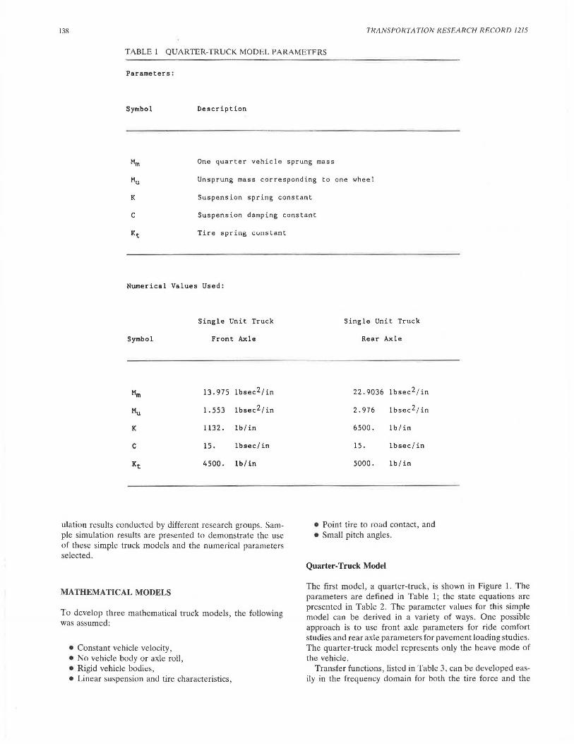
TABLE 1 QUARTER-TRUCK MODEL PARAMETERS

Parameters :

Symbol Description

One quarter vehicle sprung mass

Unsprung mass corresponding to one wheel

K Suspension spring constant

c Suspension damping constant

Tire spring constant

Numerical Values Used :

Single Unit Truck

Symbol Front Axle

Mm 13 . 975 lbsec2/in

Mu 1.553 lbsec2 / i n

K 1132. lb/in

c 15 . lbsec/in

Kt 4500. lb/in

ulation results conducted by different research groups. Sam­ple simulation results are presented to demonstrate the use of these simple truck models and the numerical parameters selected.

MATHEMATICAL MODELS

To develop three mathematical truck models, the following was assumed:

• Constant vehicle velocity, • No vehicle body or axle roll, • Rigid vehicle bodies, • Linear suspension and tire characteristics,

Single Un i t Truck

Rear Axle

22. 903 6 lbsec 2/ in

2 . 976 lbsec 2/ in

6500. lb / in

15. lbsec/ i n

5000. lb/in

• Point tire to road contact, and • Small pitch angles.

Quarter-Truck Model

The first model, a quarter-truck, is shown in Figure 1. The parameters are defined in Table 1; the state equations are presented in Table 2. The parameter values for this simple model can be derived in a variety of ways. One possible approach is to use front axle parameters for ride comfort studies and rear axle parameters for pavement loading studies. The quarter-truck model represents only the heave mode of the vehicle.

Transfer functions, listed in Table 3, can be developed eas­ily in the frequency domain for both the tire force and the

Todd and Kulakowski

TABLE 2 QUARTER-TRUCK STATE EQUATIONS

where:

q1 - Vertical displacement of sprung mass

q2 - Vertical displacement of unsprung mass

q3 - Vertical velocity of sprung mass

q4 - Vertical velocity of unsprung mass

u - Vertical displacement of road under wheel

vertical acceleration of the sprung mass. Considerable time can be saved by using the transfer functions instead of the simulation routines to calculate the frequency responses.

Half-Single-Unit Truck Model

The second model, a half-single-unit truck with single axles, is shown in Figure 2. The parameters are defined in Table 4; the state equations are presented in Table 5. This model includes both front and rear axles, resulting in both a pitch and a heave mode of the vehicle body being incorporated in the model.

Although this model is considerably more complicated than the quarter-truck model, the transfer function method could be used to determine specific frequency responses. Computer simulations can be used to determine frequency responses for any combination of the state variables and inputs. In this

139

study, computer simulations are used to determine the half­single-unit truck frequency responses.

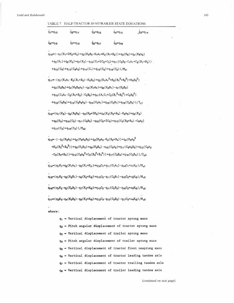
Half-Tractor Semitrailer Model

The third model, a half-tractor semitrailer, is shown in Figure 3. The parameters are defined in Table 6; the state equations are presented in Table 7. This model expands the half-single­unit truck model to include double axles and a semitrailer. The fifth wheel connecting the tractor to the semitrailer is modeled with a stiff spring and damper. This makes the fifth wheel appear nearly rigid without complicating the state equa­tions. As with the half-single-unit truck, the pitch angles have been assumed small to make the mathematical model linear.

The complexity of this model makes developing transfer functions in the frequency domain a formidable task. Com­puter simulations are used to determine all frequency responses for this model.

NUMERICAL PARAMETER VALUES

Because truck sizes and loads vary greatly, it is much more difficult to select representative parameter values for trucks than for passenger cars. The numerical data used in this paper represent a fully loaded, single-unit, single-rear-axle truck and a fully loaded, 18-wheel tractor semitrailer with the payload evenly distributed (6). These values could be used with half­truck models to study typical loaded trucks.

Because the load often is unevenly distributed, selecting parameter values for the quarter-truck model is even more difficult. Two possible approaches are presented in this paper­one for ride comfort and one for pavement loading. In both cases the numerical values are based on the single-unit-truck parameter values. The first approach uses the front axle sus­pension parameters and half of the actual unsprung mass sup-

TABLE 3 QUARTER-TRUCK TRANSFER FUNCTIONS

Transfer Functions:

Vertical acceleration of sprung mass (a1):

K s2(c + K)

Vertical tire force (Ft):

Kt2 (M9s2+c9+K)

u( s)

~~~~~~~~~~~~~~~~~~ - Kt (M 5 s2+cs+K) (Mus2+cs+k+Kt) - (Cs+k)2

r A

l B

K1

Mu 1

Kr1

FIGURE 2

~ M5 , ly

qi

c,

lq3

!ul Half-single-unit truck model.

TABLE 4 HALF-SINGLE-UNIT TRUCK MODEL PARAMETERS

Parameters:

Symbol

s

Description

One half vehicle sprung mass

One half sprung mass pitch moment

One half front axle unsprung mass

One half rear axle unsprung mass

Front suspension spring constant

Rear suspension spring constant

Front suspension damping constant

Rear suspension damping constant

Front tire spring constant

Rear tire spring constant

Horizontal distance from front axle to

sprung mass center of gravity

Horizontal distance from rear axle to

sprung mass center of gravity

·1

K2 C2

q41 Mu2

u2I

Numerical Value

36.8789 lbsec2/in

410876.4 lbsec2in

1.5528 lbsec2/in

2.9762 lbsec2in

1132. lb/in

6500. lb/in

15. lbsec/in

15. lbsec/in

4500. lb/in

5000. lb/in

149.052 in

90.948 in

K1

Q5r

TABLE 5 HALF-SINGLE-UNIT TRUCK STATE EQUATIONS

qs-( -q1 (K1+K2)+q2(K2B-K1A)+q3(K1 )+q4(K2) -q5(C1+C2)+q5(C2B-C1A)

+q7(C1)+q9(C2)J/Ms

q5-l-q1 (K1A+K2B)+q2(K2B2 -K1A2 )+q3(K1A)+q4(K2B)-q5(C1A+C2B~

+q5(C2B2-C1A2)+q7(C1A)+q9(C2B))/Iy

where :

q1 - Vertical displacement of sprung mass

q2 - Pitch angular displacement of sprung mass

q3 - Vertical displacement of front unsprung mass

q4 - Vertical displacement of rear unsprung mass

qs - Vertical velocity of sprung mass

q6 • Pitch angular velocity of sprung mass

q7 - Vertical velocity of front unsprung mass

qa - Vertical velocity of rear unsprung mass

u1 - Vertical displacement of road under front wheel

u2 - Vertical displacement of road under rear wheel

A2 84

KS cs I "'

C2

FIGURE 3 Half-tractor trailer model.

I C3 K3 C3

TABLE 6 HALF-TRACTOR SEMITRAILER MODEL PARAMETERS

Parameters:

Bz

Description Numerical Value

One halt tractor sprung mass

One half tractor sprung mass pitch moment

One half front axle unsprung mass

One half tractor rear tandem axle unsprung

mass (per axle)

Tractor front suspension spring constant

Tractor rear suspension spring constant

Tractor front suspension damping constant

Tractor rear suspension damping constant

Tractor front tire spring constant

Tractor rear tire spring constant

Horizontal distance from front axle to

tractor sprung mass center of gravity

Horizontal distance from leading rear axle

to tractor sprung mass center of gravity

Horizontal distance from fifth wheel to

tractor sprung mass center of gravity

Horizontal distance from fifth wheel to

tractor sprung mass center of gravity

One half trailer sprung mass

One half trailer spung mass pitch moment

One half trailer tandem axle unsprung mass

(per axle)

Trailer suspension spring constant

Trailer suspension damping constant

Trailer tire spring constant

Horizontal distance from fifth wheel to

trailer sprung mass center of gravity

10.401 lbsec2/in

200490.lbsec2in

1.5528 lbsec2/in

2.97~2 lbsec2in

1132.

7200.

15.

15.

lb/in

lb/in

lbsec/in

lbsec/in

4500. lb/in

9000. lb/in

60.108 in

126.342 in

177.442 in

118.662 in

81. 731

90575.5

1. 941

lbsec2/in

lbsec2in

lbsec2/in

7500. lb/in

15 lbsec/in

10000 lb/in

235.581 in

Horizontal distance from leading rear axle 220.419 in

to trailer sprung mass center of gravity

Horizontal distance from trailing rear axle 268.4

to trailer sprung mass center of gravity

in

Fifth wheel damping constant

Fifth wheel spring constant

1000. lbsec/in

100000. lb/in

Todd and Kulakowski

TABLE 7 HALF-TRACTOR SEMITRAILER STATE EQUATIONS

q,o-( -q, (K1+2K2+K5)+q2(K5B5-K1A1+K2 ( B1+B2) )+q3(K5)+q4 (KsA2)

+q5 ( K1)+q5(K2)+q7(K2)-q10CC1+2C2+Cs)+q11(C5B5-C1A1+C2(B1+B2 ) )

+q12 ( C5)+q13 ( CsA2) +q14 ( C1 )+q15( C2)+q15( C2) ) /Ms1

~11-- ( q, (K1A1 -K2(B1+B2) -K5B5)+q2(K1A1 2+K2(B1 2+B22)+KsBs2)

+q3(K5B5)+q4 (I<sBsA2) -q5(I<1A1 )+qs (I<2B1) -q7(K2B2)

+q1o(C1A1 -C2(B1+B2) -C5B5)+q11 (A1 c,+C2(B1 2+Bl)+C5B52)

+q12(C5B5)+q13(CsBsA2) -q14(C1A1 )+q15(C2B1 )+q15(C2B2) l /Iy1

q,r( q, (Ks) -q2(I<sBs) -q3(Ks+2K3)+q4(K3(B3+B4) -I<sAs)+qe (1<3)

+q9(l<J)+q10(C5) -q11 (C5B5) -q12(C5+2C3)+q13(C3(B3+B4) -CsA2)

+q17(C3)+q15(C3) l/Ms2

~13-- ( · q1 (I<sA2)+q2(I<sA2Bs)+q3(KsA2·K3(B3+B4) )+q4(KsAi

+K3(B32+B42))+q9(K3B3)+q9(K3B4)-Q1o(CsA2)+q11(CsA2B5)+q12(CsA2

-C3(B3+B4) )+q13(CsA22+C3(Bi+B/) )+q17(C3B3)+q1e(C3B4) l /Iy2

where :

q1 - Vertical displacement of tractor sprung mass

q:i - Pitch angular displacement of tractor sprung mass

q3 - Vertical displacement of trailer sprung mass

q4 - Pitch angular displacement of trailer sprung mass

q5 - Vertical displacement of tractor front unsprung mass

q5 - Vertical displacement of tractor leading tandem axle

q7 - Vertical displacement of tractor trailing tandem axle

qs - Vertical displacement of trailer leading tandem axle

(continued on next page)

143

144 TRANSPORTATION RESEARCH RECORD 1215

TABLE 7 (continued)

q9 - Vertical displacement of trailer trailing tandem axle

q10 - Vertical velocity of tractor sprung mass

q11 - Pitch angular velocity of tractor sprung mass

q12 - Vertical velocity of trailer sprung mass

q13 - Pitch angular velocity of trailer sprung mass

q14 - Vertical velocity of tractor front unsprung mass

q15 - Vertical velocity of tractor leading tandem axle

q19 - Vertical velocity of tractor trailing tandem axle

q17 - Vertical velocity of trailer leading tandem axle

q18 - Vertical velocity of trailer trailer tandem axle

u1 - Vertical road displacement under tractor front wheel

~ - Vertical road displacement under tractor leading rear wheel

u3 - Vertical road displacement under tractor trailing rear wheel

~ - Vertical road displacement under trailer leading wheel

U5 - Vertical road displacement under trailer trailing wheel

ported by the front axle. The second approach uses the rear axle suspension parameters and half of the actual unsprung mass supported by the rear axle.

COMPUTER SIMULA TIO NS

A Fortran simulation routine was written for an IBM XT or compatible personal computer. To perform the different tasks involved in digital simulation, the program was divided into several subroutines. An integration subroutine performed the numerical integration of the state equations. For this study a constant time step, fourth-order, Runga-Kutta algorithm was used (7). State equation subroutines were created for each model so that the desired model could be selected when the program was compiled . An input subroutine defined the dif­ferent road profiles. All subroutines were controlled by a main program that allowed the user to specify the simulation start time, end time, output interval, and time step.

As with any digital computer simulation, the integration time step must be selected carefully . A large time step can cause the results to be inaccurate and often unstable. A small time step causes the simulation program to use excessive com­puter time. The time step selection involves a compromise between speed and accuracy. The time step also depends on the vehicle parameters and the type of input used . Consid­erable care must be taken when selecting the time step for a fixed time step integration algorithm. A variable time step can achieve good results with a minimum of computer time.

APPLICATIONS

The primary application of these three truck models is to predict both ride comfort and dynamic pavement loading. Ride comfort is often determined from the vertical acceler­ation of the sprung mass. Using the models, acceleration fre­quency response and root mean square (RMS) acceleration can be calculated. Tire force frequency responses and dynamic impact factors (DIFs) can be determined to predict pavement loading.

The truck models were tested using two types of road pro­files . A sinusoidal road profile was used to determine fre­quency responses. Actual road profiles were used to calculate RMS acceleration and DIF.

The sinusoidal road profile used in this study is defined by

U;(t) = (.1 inch) sin (2 TJf (t - td;))

where

U; = road elevation under wheel i (in.), f = frequency (Hz), t = time (sec) , and

td; = time delay between axles (sec).

(1)

Simulations were run using frequencies between 0 and 25 Hz and a vehicle velocity of 60 ft/sec . The resulting steady-state amplitudes were plotted as a function of frequency to obtain a frequency response plot. Transfer functions were used for the quarter-truck model.

The road profile used in this study is shown in Figure 4.

Todd and Kulakowski 145

0

-0 .1

-0.2

n lJ) QJ -0.3 r u c \_) -0. "1 z 0

I- -0.5 <! > w _J

w -0.6

_J

<! u I- -0 . 7 a w >

-0.8

-0.9

-1

0 "10 80 120 160 200 2"10 280

HORIZONTAL DISTANCE (feet]

FIGURE 4 Road profile.

This profile is from a medium-roughness road having a quarter­car roughness index of 105 in./mile. The RMS acceleration is calculated from Equation 2. The DIF is calculated from Equation 3.

RMS = [ (~ ~ a~) f 2

where

RMS N= a. =

I

root mean square acceleration, total number of data points, and acceleration at ith time step.

DIF = ({;[~ (F; - F)2]/[(N - 1) * F2]}) 112

where

DIF = dynamic impact factor, F; = tire force at ith time step, N = total number of data points, and F = mean tire force.

RESULTS

Ride Comfort

(2)

(3)

The sprung mass, vertical acceleration frequency responses for each model are shown in Figures 5 through 7. Comparison

of Figures 5 and 6 shows the vertical acceleration frequency response of the quarter-truck model using the front axle parameters to be similar to frequency response of the half­single-unit truck model. The resonant peaks predicted by the quarter-truck model occur at similar frequencies but have different amplitudes than those of the half-single-unit truck model.

The RMS vertical accelerations for each model, calculated using the actual road profile, came to 13.35 for the quarter­truck (front axle); 9.01, half-single-unit truck; and 22.36, half­tractor semitrailer. The lower the RMS, the smoother the ride. As might be expected from the frequency responses, the quarter-truck model predicts a higher RMS acceleration.

Pavement Loading

The vertical tire force frequency responses for each axle of each model are shown in Figures 8 through 11. The quarter­truck model using only rear-axle parameters predicts resonant peaks near 2 and 10 Hz. The half-single-unit truck shows similar resonant peaks, but the 2-Hz peak has a larger ampli­tude than that of the quarter-truck model.

Table 8 lists the DIF for each model determined from the actual road profile. The lower the DIF, the less pavement loading. The quarter-truck model prediction is considerably higher than the DIF predicted by the half-single-unit truck model. Thus, the simpler model overestimates pavement

1 . 8

1 7

1.6

" 1.5 Ill

' 1 . 4 Ill

' ,... 1.3 u w 1.2 0 :::)

I- 1.1 - " ...J Ill

1 a. 'O :::? c <( IO

0.9 Ill 0 ::J <( 0 0 .c 0.8 a t---..u 0.7 z 0

I-0.6

<( a 0.5 w ...J w 0.4 u u 0.3 <(

0.2

0.1

0

0 4 8 12 16 20 24

FREQUENCY (HERTZ)

FIGURE 5 Quarter-truck model sprung mass vertical acceleration frequency response using single-unit truck front &)'le parameters.

1.8

1.7

1.6

" 1 . 5 Ill

' 1 . 4 Ill

' r 1.3 u w 1.2 0 :::) I- 1 . 1 - " ...J (/)

1 a. 'O :::? c <( IO

0.9 Ill 0 ::J <( 0 0 .c 0.8 a t---..u 0 . 7 z 0

I-0.6

<( a 0.5 w ...J w 0.4 u u 0.3 <(

0.2

0.1

0

0 4 8 12 16 20 24

FREQUENCY (HERTZ)

FIGURE 6 Half-single-unit truck model sprung mass vertical acceleration frequency response.

1.8

1 7

1.6

n 1.5 lfl .... 1 . 4 lfl .... ,....

1.3 LI

w 1.2 0 :::)

I- 1.1 -n _J lfl a. 'O 1 :2 c < IO 0.9 lfl 0 :::> <( 0 0.8 o.c a: I-..._ LI 0.7 z 0

I-0.6

<( a: 0.5 w _J

w 0.4 u u 0.3 <(

0.2

0.1

0

0 4 8 12 16 20 24

FREQUENCY (HERTZ)

FIGURE 7 Half-tractor semitrailer model tractor sprung mass vertical acceleration frequency response.

170

150

150

n 140 c

130 .... .D

u 120

w 110 0 :::) I- n 100 - lfl _J 'O a. c 90 :2 IO <( lfl

:::> 80 0 0 <( .c 0 I- 70 CI u .... w 50 u a: 0 50 u. w 40 CI

I- 30

20

10

0

0 4 8 12 16 20 24

FREQUENCY (HERTZ)

FIGURE 8 Quarter-truck model tire force frequency response using single-unit rear axle parameters.

170

160

150

140

n 130 c

' 120

.0

u 110

Wn 100 0 If) ::::iu f- c 90 - IO __J If) a. ::J 80 :::!: 0 4: .c

f- 70 Ou 4: 0 60 a: ' w 50 u a: 0 40 u_

30

20

10

0

0 4 8 12

FREQUENCY (HERTZ)

FIGURE 9 Half-single-unit truck model tire force frequency response.

170

160

150

140

n 130 c:

' 120 .0

u 110

wn 100 0 If) :JD f- c: 90 :i IO a. (/) :::!: ::J 80 4: 0 .c 0 f-4: u

70 0 60 CI

' w 50 u

a: 0 40 u_

30

20

10

0

0 4 8 12

16

16

FREQUENCY (HERTZ)

FIGURE 10 Half-tractor semitrailer model tractor tire force frequency responses.

0 FRONT AXLE

+REAR AXLE

20 24

0 FRONT AXLE

+LEADING REAR AXLE

<)TRAILING REAR AXLE

20 24

Todd and Kulakowski 149

170

160 0 LEAD I NG AXLE

150

140 + TRAIL I NG AXLE

n 130 c ...... 120 D

u 110

wn 100 0 tn :::> 'O I- c 90 ::::i IO Cl. Ill

80 ~ :i < 0 .c 0 I-<u

70

0 60 II ...... w so u II 0 40 u..

30

20

10

0

0 4 8 12 16 20 24

FREQUENCY (HERTZJ

FIGURE 11 Half-tractor semitrailer model trailer lire force frequency responses.

TABLE 8 DYNAMIC IMPACT FACTORS FOR ACTUAL ROAD PROFILE

Axle Number

2

3

4

5

Quarter-Truck (Rear Axle)

. 142

--- Not applicable

loading, and a more complex half-truck model has to be used if more accurate results are needed.

CONCLUSIONS

Large complicated simulation programs should not be nec­essary for most studies concerning the vertical dynamics of

Half-Single Unit Truck

.030

.071

Half-Tractor Semitrailer

.029

.042

.039

.036

.035

heavy trucks. Simple two-dimensional truck models can be used with personal computers to predict ride quality and pave­ment loading. The quarter-truck model can be used as an initial estimate by selecting the parameters properly. For more accurate results that include pitching motion, the half-single­unit truck and the half-tractor semitrailer models can be used . With standardized parameter values, uniform simulations could be performed by different research groups to allow for com­parison of the results of different studies.

150

REFERENCES

1. R. R. Hegmon. Tire-Pavement Interaction. Public Roads, Vol. 51, No. 1, 1987, pp. 5-11.

2. T. D. Gillespie, C. MacAdam, G. T. Hu, J. Bernard, and C. Winkler. Truck and Tractor-Trailer Dynamic Response Simula­tion. FHWA/RD-79-123,124,125,126. University of Michigan, Highway Safety Research Institute, FHWA, U.S. Department of Transportation, Washington, D.C., 1979.

3. G. Rill. Vehicle Dynamics in Real-Time Simulation. In The Dynamics of Vehicles 011 Roads and Tracks, In Proc., 10th IA VSD Symposium, Prague, 1987, pp. 337-347.

4. G. T. Hu. Truck and Tractor Trailer Dynamic Response Simula­tion, T3DRS:Vl. UM-HSRI-79-38-2; FHWA/RD-78/126. Univer­sity of Michigan, Highway Safety Research Institute, FHWA, U.S. Department of Transportation, Washington, D.C., 1979.

TRANSPORTATION RESEARCH RECORD 1215

5. Standard Practice for Simulating Vehicular Response to Longi­tudinal Profiles of a Vehicular Trnveled S11rfar.i" F.1170-R7. A nn.ual Book of ASTM Standards, Section 4, Vol. 04.03, 1988.

6. G. S. Alves. Computer Simulation of Truck Rollover Performance on Horizontal Curves. Master's thesis. Pennsylvania State Uni­versity, University Park, 1988.

7. J. M. Smith. Mathematica/ Modeling and Digital Simulation for Engineers and Scientists, 2nd ed. John Wiley & Sons, New York, 1987.

Publication of this paper sponsored by Committee on Surface Prop­erties-Vehicle Interaction.