Contents

1 Singular Value Decomposition (SVD) 21.1 Singular Vectors . . . . . . . . . . . . . . . . . . . . . . . . . . . . . . . . . 31.2 Singular Value Decomposition (SVD) . . . . . . . . . . . . . . . . . . . . . 71.3 Best Rank k Approximations . . . . . . . . . . . . . . . . . . . . . . . . . 81.4 Power Method for Computing the Singular Value Decomposition . . . . . . 111.5 Applications of Singular Value Decomposition . . . . . . . . . . . . . . . . 16

1.5.1 Principal Component Analysis . . . . . . . . . . . . . . . . . . . . . 161.5.2 Clustering a Mixture of Spherical Gaussians . . . . . . . . . . . . . 161.5.3 An Application of SVD to a Discrete Optimization Problem . . . . 221.5.4 SVD as a Compression Algorithm . . . . . . . . . . . . . . . . . . . 241.5.5 Spectral Decomposition . . . . . . . . . . . . . . . . . . . . . . . . 241.5.6 Singular Vectors and ranking documents . . . . . . . . . . . . . . . 25

1.6 Bibliographic Notes . . . . . . . . . . . . . . . . . . . . . . . . . . . . . . . 271.7 Exercises . . . . . . . . . . . . . . . . . . . . . . . . . . . . . . . . . . . . . 28

1

1 Singular Value Decomposition (SVD)

The singular value decomposition of a matrix A is the factorization of A into theproduct of three matrices A = UDV T where the columns of U and V are orthonormal andthe matrix D is diagonal with positive real entries. The SVD is useful in many tasks. Herewe mention some examples. First, in many applications, the data matrix A is close to amatrix of low rank and it is useful to find a low rank matrix which is a good approximationto the data matrix . We will show that from the singular value decomposition of A, wecan get the matrix B of rank k which best approximates A; in fact we can do this for everyk. Also, singular value decomposition is defined for all matrices (rectangular or square)unlike the more commonly used spectral decomposition in Linear Algebra. The readerfamiliar with eigenvectors and eigenvalues (we do not assume familiarity here) will alsorealize that we need conditions on the matrix to ensure orthogonality of eigenvectors. Incontrast, the columns of V in the singular value decomposition, called the right singularvectors of A, always form an orthogonal set with no assumptions on A. The columnsof U are called the left singular vectors and they also form an orthogonal set. A simpleconsequence of the orthogonality is that for a square and invertible matrix A, the inverseof A is V D−1UT , as the reader can verify.

To gain insight into the SVD, treat the rows of an n × d matrix A as n points in ad-dimensional space and consider the problem of finding the best k-dimensional subspacewith respect to the set of points. Here best means minimize the sum of the squares of theperpendicular distances of the points to the subspace. We begin with a special case ofthe problem where the subspace is 1-dimensional, a line through the origin. We will seelater that the best-fitting k-dimensional subspace can be found by k applications of thebest fitting line algorithm. Finding the best fitting line through the origin with respectto a set of points xi|1 ≤ i ≤ n in the plane means minimizing the sum of the squareddistances of the points to the line. Here distance is measured perpendicular to the line.The problem is called the best least squares fit.

In the best least squares fit, one is minimizing the distance to a subspace. An alter-native problem is to find the function that best fits some data. Here one variable y is afunction of the variables x1, x2, . . . , xd and one wishes to minimize the vertical distance,i.e., distance in the y direction, to the subspace of the xi rather than minimize the per-pendicular distance to the subspace being fit to the data.

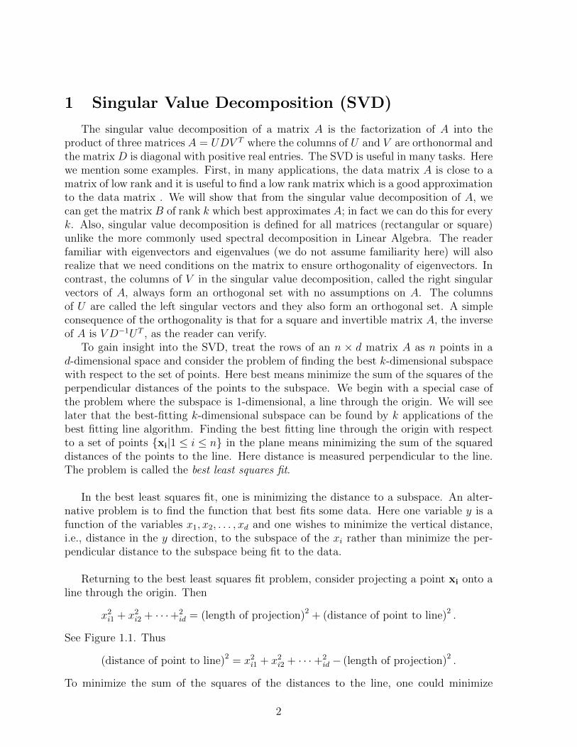
Returning to the best least squares fit problem, consider projecting a point xi onto aline through the origin. Then

x2i1 + x2

i2 + · · ·+2id = (length of projection)2 + (distance of point to line)2 .

See Figure 1.1. Thus

(distance of point to line)2 = x2i1 + x2

i2 + · · ·+2id − (length of projection)2 .

To minimize the sum of the squares of the distances to the line, one could minimize

2

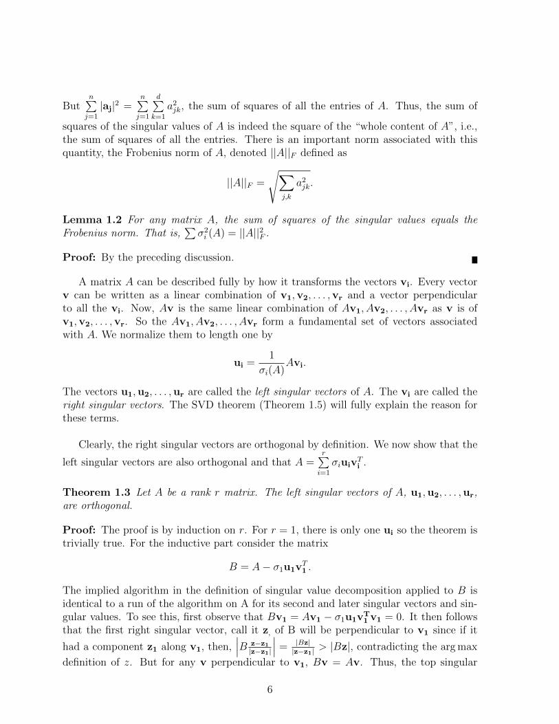
v

xi

αi

βi

xj

βj

αj

Min∑α2

Equivalent to

Max∑β2

Figure 1.1: The projection of the point xi onto the line through the origin in the directionof v

n∑i=1

(x2i1 + x2

i2 + · · ·+2id) minus the sum of the squares of the lengths of the projections of

the points to the line. However,n∑i=1

(x2i1 + x2

i2 + · · ·+2id) is a constant (independent of the

line), so minimizing the sum of the squares of the distances is equivalent to maximizingthe sum of the squares of the lengths of the projections onto the line. Similarly for best-fitsubspaces, we could maximize the sum of the squared lengths of the projections onto thesubspace instead of minimizing the sum of squared distances to the subspace.

The reader may wonder why we minimize the sum of squared perpendicular distancesto the line. We could alternatively have defined the best-fit line to be the one whichminimizes the sum of perpendicular distances to the line. There are examples wherethis definition gives a different answer than the line minimizing the sum of perpendiculardistances squared. [The reader could construct such examples.] The choice of the objectivefunction as the sum of squared distances seems arbitrary and in a way it is. But the squarehas many nice mathematical properties - the first of these is the use of Pythagoras theoremabove to say that this is equivalent to maximizing the sum of squared projections. We willsee that in fact we can use the Greedy Algorithm to find best-fit k dimensional subspaces(which we will define soon) and for this too, the square is important. The reader shouldalso recall from Calculus that the best-fit function is also defined in terms of least-squaresfit. There too, the existence of nice mathematical properties is the motivation for thesquare.

1.1 Singular Vectors

We now define the singular vectors of an n× d matrix A. Consider the rows of A as npoints in a d-dimensional space. Consider the best fit line through the origin. Let v be a

3

unit vector along this line. The length of the projection of ai, the ith row of A, onto v is|ai · v|. From this we see that the sum of length squared of the projections is |Av|2. Thebest fit line is the one maximizing |Av|2 and hence minimizing the sum of the squareddistances of the points to the line.

With this in mind, define the first singular vector, v1, of A, which is a column vector,as the best fit line through the origin for the n points in d-space that are the rows of A.Thus

v1 = arg max|v|=1|Av|.

The value σ1 (A) = |Av1| is called the first singular value of A. Note that σ21 is the

sum of the squares of the projections of the points to the line determined by v1.

The greedy approach to find the best fit 2-dimensional subspace for a matrix A, takesv1 as the first basis vector for the 2-dimenional subspace and finds the best 2-dimensionalsubspace containing v1. The fact that we are using the sum of squared distances will againhelp. For every 2-dimensional subspace containing v1, the sum of squared lengths of theprojections onto the subspace equals the sum of squared projections onto v1 plus the sumof squared projections along a vector perpendicular to v1 in the subspace. Thus, insteadof looking for the best 2-dimensional subspace containing v1, look for a unit vector, callit v2, perpendicular to v1 that maximizes |Av|2 among all such unit vectors. Using thesame greedy strategy to find the best three and higher dimensional subspaces, definesv3,v4, . . . in a similar manner. This is captured in the following definitions. There is noapriori guarantee that the greedy algorithm gives the best fit. But, in fact, the greedyalgorithm does work and yields the best-fit subspaces of every dimension as we will show.

The second singular vector, v2, is defined by the best fit line perpendicular to v1

v2 = arg maxv⊥v1,|v|=1

|Av| .

The value σ2 (A) = |Av2| is called the second singular value of A. The third singularvector v3 is defined similarly by

v3 = arg maxv⊥v1,v2,|v|=1

|Av|

and so on. The process stops when we have found

v1,v2, . . . ,vr

as singular vectors andarg max

v⊥v1,v2,...,vr|v|=1

|Av| = 0.

If instead of finding v1 that maximized |Av| and then the best fit 2-dimensionalsubspace containing v1, we had found the best fit 2-dimensional subspace, we might have

4

done better. This is not the case. We now give a simple proof that the greedy algorithmindeed finds the best subspaces of every dimension.

Theorem 1.1 Let A be an n × d matrix where v1,v2, . . . ,vr are the singular vectorsdefined above. For 1 ≤ k ≤ r, let Vk be the subspace spanned by v1,v2, . . . ,vk. Then foreach k, Vk is the best-fit k-dimensional subspace for A.

Proof: The statement is obviously true for k = 1. For k = 2, let W be a best-fit 2-dimensional subspace for A. For any basis w1,w2 of W , |Aw1|2 + |Aw2|2 is the sum ofsquared lengths of the projections of the rows of A onto W . Now, choose a basis w1,w2

of W so that w2 is perpendicular to v1. If v1 is perpendicular to W , any unit vector in Wwill do as w2. If not, choose w2 to be the unit vector in W perpendicular to the projectionof v1 onto W. Since v1 was chosen to maximize |Av1|2, it follows that |Aw1|2 ≤ |Av1|2.Since v2 was chosen to maximize |Av2|2 over all v perpendicular to v1, |Aw2|2 ≤ |Av2|2.Thus

|Aw1|2 + |Aw2|2 ≤ |Av1|2 + |Av2|2.Hence, V2 is at least as good as W and so is a best-fit 2-dimensional subspace.

For general k, proceed by induction. By the induction hypothesis, Vk−1 is a best-fitk-1 dimensional subspace. Suppose W is a best-fit k-dimensional subspace. Choose abasis w1,w2, . . . ,wk of W so that wk is perpendicular to v1,v2, . . . ,vk−1. Then

|Aw1|2 + |Aw2|2 + · · ·+ |Awk|2 ≤ |Av1|2 + |Av2|2 + · · ·+ |Avk−1|2 + |Awk|2

since Vk−1 is an optimal k -1 dimensional subspace. Since wk is perpendicular tov1,v2, . . . ,vk−1, by the definition of vk, |Awk|2 ≤ |Avk|2. Thus

|Aw1|2 + |Aw2|2 + · · ·+ |Awk−1|2 + |Awk|2 ≤ |Av1|2 + |Av2|2 + · · ·+ |Avk−1|2 + |Avk|2,

proving that Vk is at least as good as W and hence is optimal.

Note that the n-vector Avi is really a list of lengths (with signs) of the projections ofthe rows of A onto vi. Think of |Avi| = σi(A) as the “component” of the matrix A alongvi. For this interpretation to make sense, it should be true that adding up the squares ofthe components of A along each of the vi gives the square of the “whole content of thematrix A”. This is indeed the case and is the matrix analogy of decomposing a vectorinto its components along orthogonal directions.

Consider one row, say aj, of A. Since v1,v2, . . . ,vr span the space of all rows of A,

aj · v = 0 for all v perpendicular to v1,v2, . . . ,vr. Thus, for each row aj,r∑i=1

(aj · vi)2 =

|aj|2. Summing over all rows j,

n∑j=1

|aj|2 =n∑j=1

r∑i=1

(aj · vi)2 =

r∑i=1

n∑j=1

(aj · vi)2 =

r∑i=1

|Avi|2 =r∑i=1

σ2i (A).

5

Butn∑j=1

|aj|2 =n∑j=1

d∑k=1

a2jk, the sum of squares of all the entries of A. Thus, the sum of

squares of the singular values of A is indeed the square of the “whole content of A”, i.e.,the sum of squares of all the entries. There is an important norm associated with thisquantity, the Frobenius norm of A, denoted ||A||F defined as

||A||F =

√∑j,k

a2jk.

Lemma 1.2 For any matrix A, the sum of squares of the singular values equals theFrobenius norm. That is,

∑σ2i (A) = ||A||2F .

Proof: By the preceding discussion.

A matrix A can be described fully by how it transforms the vectors vi. Every vectorv can be written as a linear combination of v1,v2, . . . ,vr and a vector perpendicularto all the vi. Now, Av is the same linear combination of Av1, Av2, . . . , Avr as v is ofv1,v2, . . . ,vr. So the Av1, Av2, . . . , Avr form a fundamental set of vectors associatedwith A. We normalize them to length one by

ui =1

σi(A)Avi.

The vectors u1,u2, . . . ,ur are called the left singular vectors of A. The vi are called theright singular vectors. The SVD theorem (Theorem 1.5) will fully explain the reason forthese terms.

Clearly, the right singular vectors are orthogonal by definition. We now show that the

left singular vectors are also orthogonal and that A =r∑i=1

σiuivTi .

Theorem 1.3 Let A be a rank r matrix. The left singular vectors of A, u1,u2, . . . ,ur,are orthogonal.

Proof: The proof is by induction on r. For r = 1, there is only one ui so the theorem istrivially true. For the inductive part consider the matrix

B = A− σ1u1vT1 .

The implied algorithm in the definition of singular value decomposition applied to B isidentical to a run of the algorithm on A for its second and later singular vectors and sin-gular values. To see this, first observe that Bv1 = Av1 − σ1u1v

T1 v1 = 0. It then follows

that the first right singular vector, call it z, of B will be perpendicular to v1 since if it

had a component z1 along v1, then,∣∣∣B z−z1|z−z1|

∣∣∣ = |Bz||z−z1| > |Bz|, contradicting the arg max

definition of z. But for any v perpendicular to v1, Bv = Av. Thus, the top singular

6

vector of B is indeed a second singular vector of A. Repeating this argument shows thata run of the algorithm on B is the same as a run on A for its second and later singularvectors. This is left as an exercise.

Thus, there is a run of the algorithm that finds that B has right singular vectorsv2,v3, . . . ,vr and corresponding left singular vectors u2,u3, . . . ,ur. By the inductionhypothesis, u2,u3, . . . ,ur are orthogonal.

It remains to prove that u1 is orthogonal to the other ui. Suppose not and for somei ≥ 2, uT1ui 6= 0. Without loss of generality assume that uT1ui > 0. The proof is symmetricfor the case where uT1ui < 0. Now, for infinitesimally small ε > 0, the vector

A

(v1 + εvi

|v1 + εvi|

)=σ1u1 + εσiui√

1 + ε2

has length at least as large as its component along u1 which is

uT1 (σ1u1 + εσiui√

1 + ε2) =

(σ1 + εσiu

T1ui

) (1− ε2

2+O (ε4)

)= σ1 + εσiu

T1ui −O

(ε2)> σ1

a contradiction. Thus, u1,u2, . . . ,ur are orthogonal.

1.2 Singular Value Decomposition (SVD)

Let A be an n×dmatrix with singular vectors v1,v2, . . . ,vr and corresponding singularvalues σ1, σ2, . . . , σr. Then ui = 1

σiAvi, for i = 1, 2, . . . , r, are the left singular vectors and

by Theorem 1.5, A can be decomposed into a sum of rank one matrices as

A =r∑i=1

σiuivTi .

We first prove a simple lemma stating that two matrices A and B are identical ifAv = Bv for all v. The lemma states that in the abstract, a matrix A can be viewed asa transformation that maps vector v onto Av.

Lemma 1.4 Matrices A and B are identical if and only if for all vectors v, Av = Bv.

Proof: Clearly, if A = B then Av = Bv for all v. For the converse, suppose thatAv = Bv for all v. Let ei be the vector that is all zeros except for the ithcomponentwhich has value 1. Now Aei is the ith column of A and thus A = B if for each i, Aei = Bei.

7

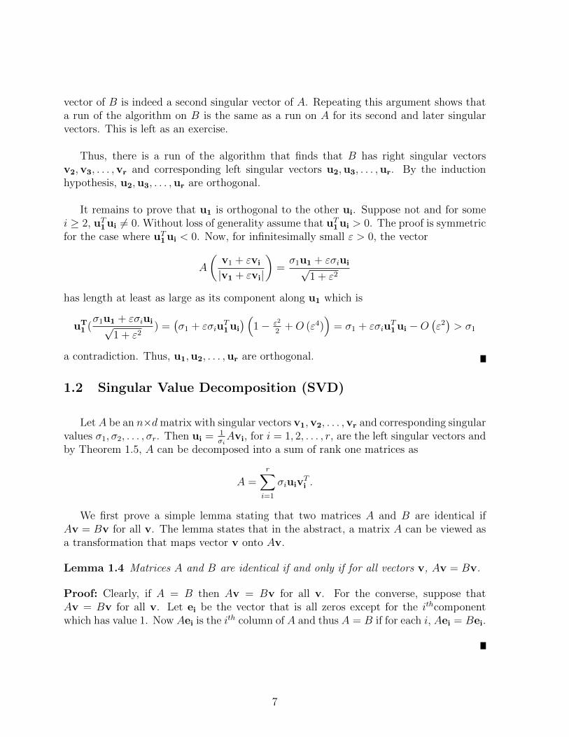
A

n× dU

n× r

D

r × rV T

r × d

=

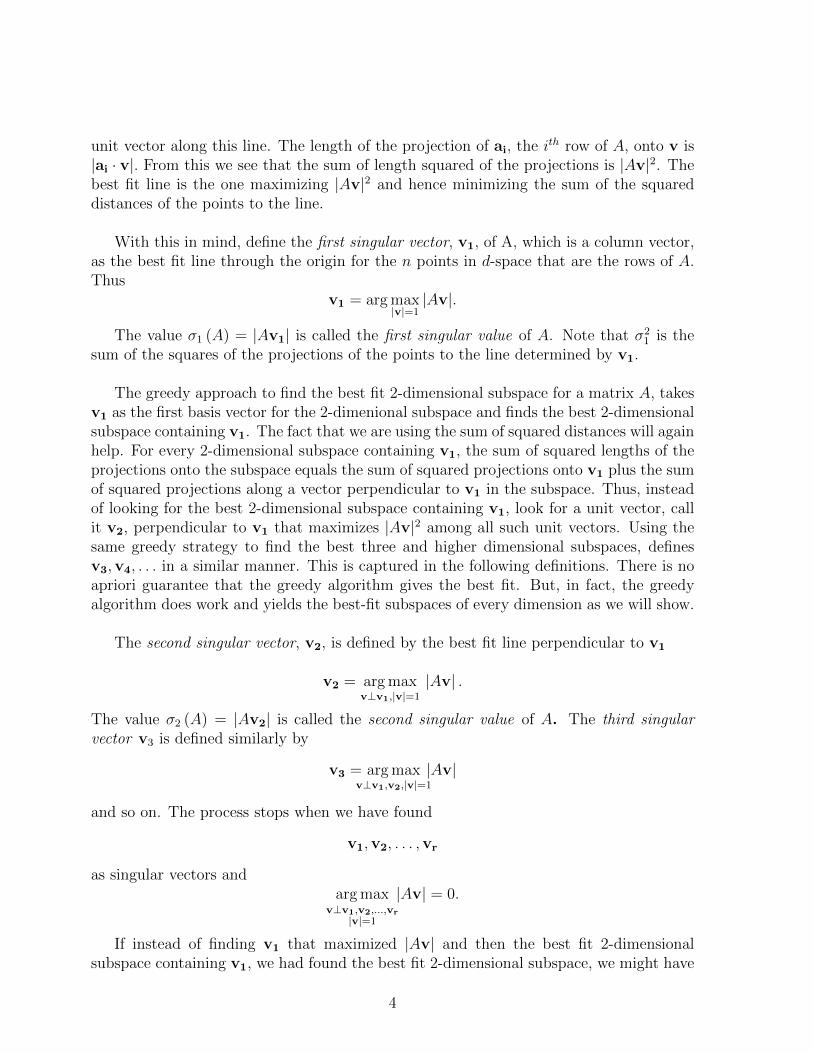
Figure 1.2: The SVD decomposition of an n× d matrix.

Theorem 1.5 Let A be an n × d matrix with right singular vectors v1,v2, . . . ,vr, leftsingular vectors u1,u2, . . . ,ur, and corresponding singular values σ1, σ2, . . . , σr. Then

A =r∑i=1

σiuivTi .

Proof: For each singular vector vj, Avj =r∑i=1

σiuivTi vj. Since any vector v can be ex-

pressed as a linear combination of the singular vectors plus a vector perpendicular to the

vi, Av =r∑i=1

σiuivTi v and by Lemma 1.4, A =

r∑i=1

σiuivTi .

The decomposition is called the singular value decomposition, SVD, of A. In matrixnotation A = UDV T where the columns of U and V consist of the left and right singularvectors, respectively, and D is a diagonal matrix whose diagonal entries are the singularvalues of A.

For any matrix A, the sequence of singular values is unique and if the singular valuesare all distinct, then the sequence of singular vectors is unique also. However, when someset of singular values are equal, the corresponding singular vectors span some subspace.Any set of orthonormal vectors spanning this subspace can be used as the singular vectors.

1.3 Best Rank k Approximations

There are two important matrix norms, the Frobenius norm denoted ||A||F and the2-norm denoted ||A||2. The 2-norm of the matrix A is given by

max|v|=1

|Av|

8

and thus equals the largest singular value of the matrix.

Let A be an n × d matrix and think of the rows of A as n points in d-dimensionalspace. The Frobenius norm of A is the square root of the sum of the squared distance ofthe points to the origin. The 2-norm is the square root of the sum of squared distancesto the origin along the direction that maximizes this quantity.

Let

A =r∑i=1

σiuivTi

be the SVD of A. For k ∈ 1, 2, . . . , r, let

Ak =k∑i=1

σiuivTi

be the sum truncated after k terms. It is clear that Ak has rank k. Furthermore, Ak isthe best rank k approximation to A when the error is measured in either the 2-norm orthe Frobenius norm.

Lemma 1.6 The rows of Ak are the projections of the rows of A onto the subspace Vkspanned by the first k singular vectors of A.

Proof: Let a be an arbitrary row vector. Since the vi are orthonormal, the projection

of the vector a onto Vk is given byk∑i=1

(a · vi)viT . Thus, the matrix whose rows are the

projections of the rows of A onto Vk is given byk∑i=1

AvivTi . This last expression simplifies

tok∑i=1

AviviT =

k∑i=1

σiuiviT = Ak.

The matrix Ak is the best rank k approximation to A in both the Frobenius and the2-norm. First we show that the matrix Ak is the best rank k approximation to A in theFrobenius norm.

Theorem 1.7 For any matrix B of rank at most k

‖A− Ak‖F ≤ ‖A−B‖F

Proof: Let B minimize ‖A−B‖2F among all rank k or less matrices. Let V be the space

spanned by the rows of B. The dimension of V is at most k. Since B minimizes ‖A−B‖2F ,

it must be that each row of B is the projection of the corresponding row of A onto V ,

9

otherwise replacing the row of B with the projection of the corresponding row of A ontoV does not change V and hence the rank of B but would reduce ‖A−B‖2

F . Since eachrow of B is the projection of the corresponding row of A, it follows that ‖A−B‖2

F isthe sum of squared distances of rows of A to V . Since Ak minimizes the sum of squareddistance of rows of A to any k-dimensional subspace, from Theorem (1.1), it follows that‖A− Ak‖F ≤ ‖A−B‖F .

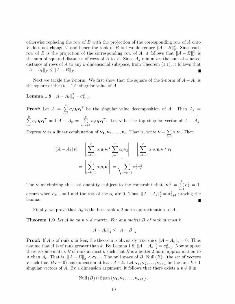
Next we tackle the 2-norm. We first show that the square of the 2-norm of A−Ak isthe square of the (k + 1)st singular value of A,

Lemma 1.8 ‖A− Ak‖22 = σ2

k+1.

Proof: Let A =r∑i=1

σiuiviT be the singular value decomposition of A. Then Ak =

k∑i=1

σiuiviT and A − Ak =

r∑i=k+1

σiuiviT . Let v be the top singular vector of A − Ak.

Express v as a linear combination of v1,v2, . . . ,vr. That is, write v =r∑i=1

αivi. Then

|(A− Ak)v| =

∣∣∣∣∣r∑

i=k+1

σiuiviT

r∑j=1

αjvj

∣∣∣∣∣ =

∣∣∣∣∣r∑

i=k+1

αiσiuiviTvi

∣∣∣∣∣=

∣∣∣∣∣r∑

i=k+1

αiσiui

∣∣∣∣∣ =

√√√√ r∑i=k+1

α2iσ

2i .

The v maximizing this last quantity, subject to the constraint that |v|2 =r∑i=1

α2i = 1,

occurs when αk+1 = 1 and the rest of the αi are 0. Thus, ‖A− Ak‖22 = σ2

k+1 proving thelemma.

Finally, we prove that Ak is the best rank k 2-norm approximation to A.

Theorem 1.9 Let A be an n× d matrix. For any matrix B of rank at most k

‖A− Ak‖2 ≤ ‖A−B‖2

Proof: If A is of rank k or less, the theorem is obviously true since ‖A− Ak‖2 = 0. Thusassume that A is of rank greater than k. By Lemma 1.8, ‖A− Ak‖2

2 = σ2k+1. Now suppose

there is some matrix B of rank at most k such that B is a better 2-norm approximation toA than Ak. That is, ‖A−B‖2 < σk+1. The null space of B, Null (B), (the set of vectorsv such that Bv = 0) has dimension at least d− k. Let v1,v2, . . . ,vk+1 be the first k + 1singular vectors of A. By a dimension argument, it follows that there exists a z 6= 0 in

Null (B) ∩ Span v1,v2, . . . ,vk+1 .

10

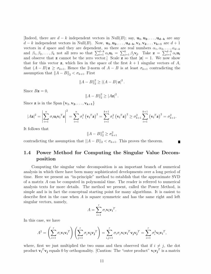
[Indeed, there are d − k independent vectors in Null(B); say, u1,u2, . . . ,ud−k are anyd − k independent vectors in Null(B). Now, u1,u2, . . . ,ud−k,v1,v2, . . .vk+1 are d + 1vectors in d space and they are dependent, so there are real numbers α1, α2, . . . , αd−kand β1, β2, . . . , βk not all zero so that

∑d−ki=1 αiui =

∑kj=1 βjvj. Take z =

∑d−ki=1 αiui

and observe that z cannot be the zero vector.] Scale z so that |z| = 1. We now showthat for this vector z, which lies in the space of the first k + 1 singular vectors of A,that (A−B) z ≥ σk+1. Hence the 2-norm of A − B is at least σk+1 contradicting theassumption that ‖A−B‖2 < σk+1. First

‖A−B‖22 ≥ |(A−B) z|2 .

Since Bz = 0,‖A−B‖2

2 ≥ |Az|2 .

Since z is in the Span v1,v2, . . . ,vk+1

|Az|2 =

∣∣∣∣∣n∑i=1

σiuiviTz

∣∣∣∣∣2

=n∑i=1

σ2i

(viTz)2

=k+1∑i=1

σ2i

(viTz)2 ≥ σ2

k+1

k+1∑i=1

(viTz)2

= σ2k+1.

It follows that‖A−B‖2

2 ≥ σ2k+1

contradicting the assumption that ||A−B||2 < σk+1. This proves the theorem.

1.4 Power Method for Computing the Singular Value Decom-position

Computing the singular value decomposition is an important branch of numericalanalysis in which there have been many sophisticated developments over a long period oftime. Here we present an “in-principle” method to establish that the approximate SVDof a matrix A can be computed in polynomial time. The reader is referred to numericalanalysis texts for more details. The method we present, called the Power Method, issimple and is in fact the conceptual starting point for many algorithms. It is easiest todescribe first in the case when A is square symmetric and has the same right and leftsingular vectors, namely,

A =r∑i=1

σiviviT .

In this case, we have

A2 =

(r∑i=1

σiviviT

)(r∑j=1

σjvjvjT

)=

r∑i,j=1

σiσjviviTvjvj

T =r∑i=1

σ2i vivi

T ,

where, first we just multiplied the two sums and then observed that if i 6= j, the dotproduct vi

Tvj equals 0 by orthogonality. [Caution: The “outer product” vivjT is a matrix

11

and is not zero even for i 6= j.] Similarly, if we take the k th power of A, again all thecross terms are zero and we will get

Ak =r∑i=1

σki viviT .

If we had σ1 > σ2, we would have

1

σk1Ak → v1v1

T .

Now we do not know σ1 beforehand and cannot find this limit, but if we just take Ak

and divide by ||Ak||F so that the Frobenius norm is normalized to 1 now, that matrixwill converge to the rank 1 matrix v1v1

T from which v1 may be computed. [This isstill an intuitive description, which we will make precise shortly. First, we cannot makethe assumption that A is square and has the same right and left singular vectors. But,B = AAT satisfies both these conditions. If again, the SVD of A is

∑i

σiuivTi , then by

direct multiplication

B = AAT =

(∑i

σiuivTi

)(∑j

σjvjuTj

)=∑i,j

σiσjuivTi vju

Tj =

∑i,j

σiσjui(vTi · vj)u

Tj

=∑i

σ2i uiu

Ti ,

since vTi vj is the dot product of the two vectors and is zero unless i = j. This is thespectral decomposition of B. Using the same kind of calculation as above,

Bk =∑i

σ2ki uiu

Ti .

As k increases, for i > 1, σ2ki /σ

2k1 goes to zero and Bk is approximately equal to

σ2k1 u1u

T1

provided that for each i > 1, σi (A) < σ1 (A).

This suggests a way of finding σ1 and u1, by successively powering B. But there aretwo issues. First, if there is a significant gap between the first and second singular valuesof a matrix, then the above argument applies and the power method will quickly convergeto the first left singular vector. Suppose there is no significant gap. In the extreme case,there may be ties for the top singular value. Then the above argument does not work.There are cumbersome ways of overcoming this by assuming a “gap” between σ1 and σ2;

12

such proofs do have the advantage that with a greater gap, better results can be proved,but at the cost of some mess. Here, instead, we will adopt a clean solution in Theorem1.11 below which states that even with ties, the power method converges to some vectorin the span of those singular vectors corresponding to the “nearly highest” singular values.

A second issue is that computing Bk costs k matrix multiplications when done ina straight-forward manner or O (log k) when done by successive squaring. Instead wecompute

Bkx

where x is a random unit length vector, the idea being that the component of x in thedirection of u1 would get multiplied by σ2

1 each time, while the component of x alongother ui would be multiplied only by σ2

i . Of course, if the component of x along u1 is zeroto start with, this would not help at all - it would always remain 0. But, this problem isfixed by picking x to be random as we show in Lemma (1.10).

Each increase in k requires multiplying B by the vector Bk−1x, which we can furtherbreak up into

Bkx = A(AT(Bk−1x

)).

This requires two matrix-vector products, involving the matrices AT and A. In manyapplications, data matrices are sparse - many entries are zero. [A leading example is thematrix of hypertext links in the web. There are more than 1010 web pages and the matrixwould be 1010by 1010. But on the average only about 10 entries per row are non-zero;so only about 1011 of the possible 1020 entries are non-zero.] Sparse matrices are oftenrepresented by giving just a linked list of the non-zero entries and their values. If Ais represented in this sparse manner, then the reader can convince him/herself that wecan a matrix vector product in time proportional to the number of nonzero entries in A.Since Bkx ≈ σ2k

1 u1(uT1 · x) is a scalar multiple of u1, u1 can be recovered from Bkx bynormalization.

We start with a technical Lemma needed in the proof of the theorem.

Lemma 1.10 Let (x1, x2, . . . , xd) be a unit d-dimensional vector picked at random fromthe set x : |x| ≤ 1. The probability that |x1| ≥ 1

20√d

is at least 9/10.

Proof: We first show that for a vector v picked at random with |v| ≤ 1, the probabilitythat v1 ≥ 1

20√d

is at least 9/10. Then we let x = v/|v|. This can only increase the valueof v1, so the result follows.

Let α = 120√d. The probability that |v1| ≥ α equals one minus the probability that

|v1| ≤ α. The probability that |v1| ≤ α is equal to the fraction of the volume of the unitsphere with |v1| ≤ α. To get an upper bound on the volume of the sphere with |v1| ≤ α,consider twice the volume of the unit radius cylinder of height α. The volume of the

13

120√d

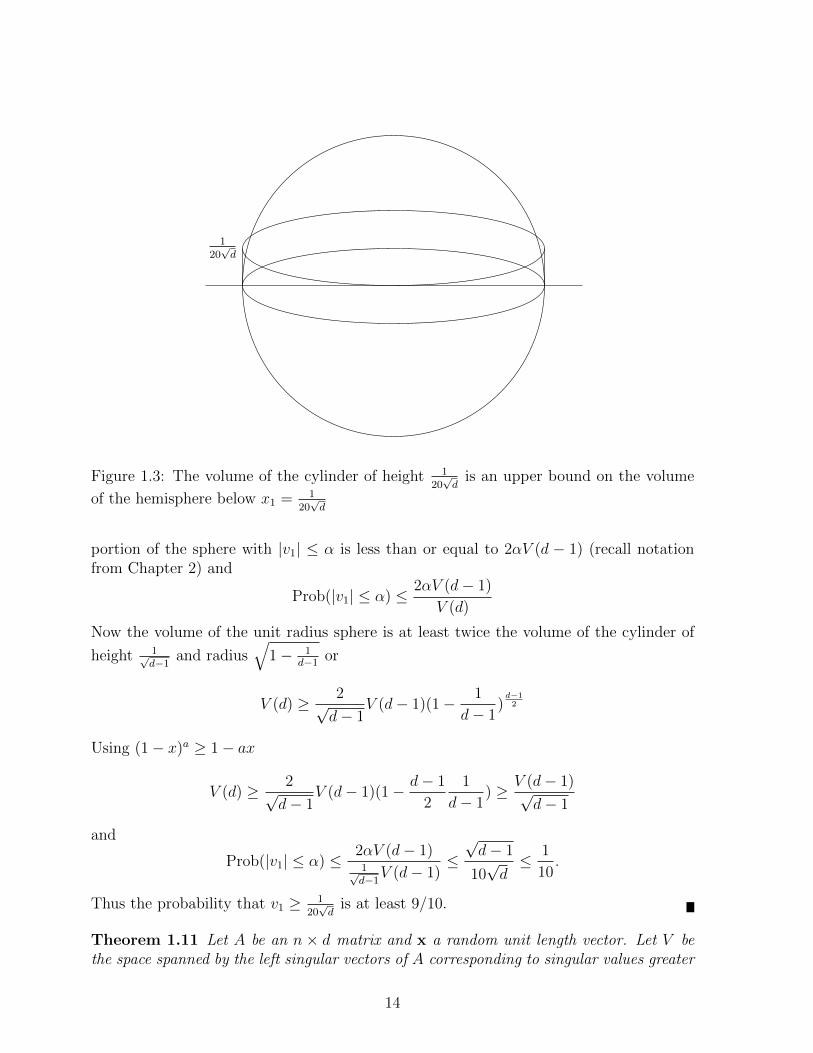
Figure 1.3: The volume of the cylinder of height 120√d

is an upper bound on the volume

of the hemisphere below x1 = 120√d

portion of the sphere with |v1| ≤ α is less than or equal to 2αV (d − 1) (recall notationfrom Chapter 2) and

Prob(|v1| ≤ α) ≤ 2αV (d− 1)

V (d)

Now the volume of the unit radius sphere is at least twice the volume of the cylinder of

height 1√d−1

and radius√

1− 1d−1

or

V (d) ≥ 2√d− 1

V (d− 1)(1− 1

d− 1)d−12

Using (1− x)a ≥ 1− ax

V (d) ≥ 2√d− 1

V (d− 1)(1− d− 1

2

1

d− 1) ≥ V (d− 1)√

d− 1

and

Prob(|v1| ≤ α) ≤ 2αV (d− 1)1√d−1

V (d− 1)≤√d− 1

10√d≤ 1

10.

Thus the probability that v1 ≥ 120√d

is at least 9/10.

Theorem 1.11 Let A be an n × d matrix and x a random unit length vector. Let V bethe space spanned by the left singular vectors of A corresponding to singular values greater

14

than (1− ε)σ1. Let k be Ω(

ln(d/ε)ε

). Let w be unit vector after k iterations of the power

method, namely,

w =

(AAT

)kx∣∣∣(AAT )k x∣∣∣ .

The probability that w has a component of at least ε perpendicular to V is at most 1/10.

Proof: Let

A =r∑i=1

σiuivTi

be the SVD of A. If the rank of A is less than d, then complete u1,u2, . . .ur into abasis u1,u2, . . .ud of d-space. Write x in the basis of the ui

′s as

x =n∑i=1

ciui.

Since (AAT )k =d∑i=1

σ2ki uiu

Ti , it follows that (AAT )kx =

d∑i=1

σ2ki ciui. For a random unit

length vector x picked independent of A, the ui are fixed vectors and picking x at randomis equivalent to picking random ci. From Lemma 1.10, |c1| ≥ 1

20√d

with probability at

least 9/10.

Suppose that σ1, σ2, . . . , σm are the singular values of A that are greater than or equalto (1− ε)σ1 and that σm+1, . . . , σn are the singular values that are less than (1− ε)σ1.Now

|(AAT )kx|2 =

∣∣∣∣∣n∑i=1

σ2ki ciui

∣∣∣∣∣2

=n∑i=1

σ4ki c

2i ≥ σ4k

1 c21 ≥

1

400dσ4k

1 ,

with probability at least 9/10. Here we used the fact that a sum of positive quantities isat least as large as its first element and the first element is greater than or equal to 1

400dσ4k

1

with probability at least 9/10. [Note: If we did not choose x at random in the begin-ning and use Lemma 1.10, c1 could well have been zero and this argument would not work.]

The component of |(AAT )kx|2 perpendicular to the space V is

d∑i=m+1

σ4ki c

2i ≤ (1− ε)4k σ4k

1

d∑i=m+1

c2i ≤ (1− ε)4k σ4k

1 ,

since∑n

i=1 c2i = |x| = 1. Thus, the component of w perpendicular to V is at most

(1− ε)2kσ2k1

120√dσ2k

1

= O(√d(1− ε)2k) = O(

√de−2εk) = O

(√de−Ω(ln(d/ε))

)= O(ε)

as desired.

15

1.5 Applications of Singular Value Decomposition

1.5.1 Principal Component Analysis

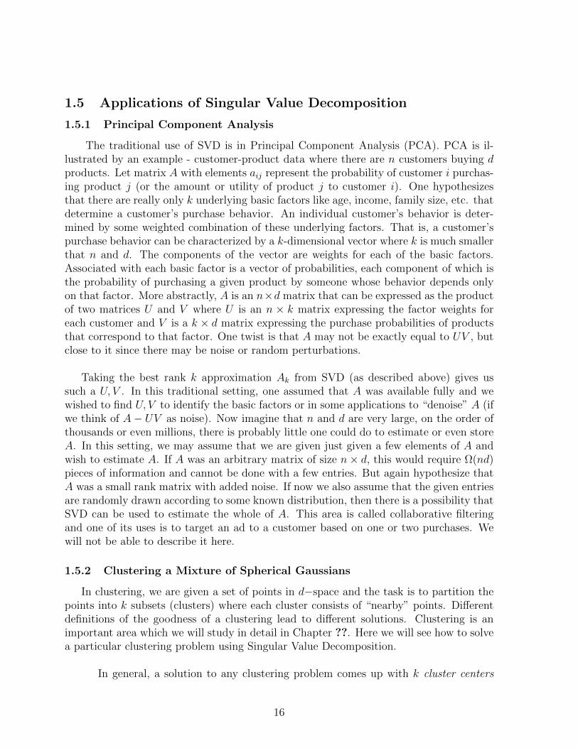
The traditional use of SVD is in Principal Component Analysis (PCA). PCA is il-lustrated by an example - customer-product data where there are n customers buying dproducts. Let matrix A with elements aij represent the probability of customer i purchas-ing product j (or the amount or utility of product j to customer i). One hypothesizesthat there are really only k underlying basic factors like age, income, family size, etc. thatdetermine a customer’s purchase behavior. An individual customer’s behavior is deter-mined by some weighted combination of these underlying factors. That is, a customer’spurchase behavior can be characterized by a k-dimensional vector where k is much smallerthat n and d. The components of the vector are weights for each of the basic factors.Associated with each basic factor is a vector of probabilities, each component of which isthe probability of purchasing a given product by someone whose behavior depends onlyon that factor. More abstractly, A is an n×d matrix that can be expressed as the productof two matrices U and V where U is an n × k matrix expressing the factor weights foreach customer and V is a k × d matrix expressing the purchase probabilities of productsthat correspond to that factor. One twist is that A may not be exactly equal to UV , butclose to it since there may be noise or random perturbations.

Taking the best rank k approximation Ak from SVD (as described above) gives ussuch a U, V . In this traditional setting, one assumed that A was available fully and wewished to find U, V to identify the basic factors or in some applications to “denoise” A (ifwe think of A− UV as noise). Now imagine that n and d are very large, on the order ofthousands or even millions, there is probably little one could do to estimate or even storeA. In this setting, we may assume that we are given just given a few elements of A andwish to estimate A. If A was an arbitrary matrix of size n× d, this would require Ω(nd)pieces of information and cannot be done with a few entries. But again hypothesize thatA was a small rank matrix with added noise. If now we also assume that the given entriesare randomly drawn according to some known distribution, then there is a possibility thatSVD can be used to estimate the whole of A. This area is called collaborative filteringand one of its uses is to target an ad to a customer based on one or two purchases. Wewill not be able to describe it here.

1.5.2 Clustering a Mixture of Spherical Gaussians

In clustering, we are given a set of points in d−space and the task is to partition thepoints into k subsets (clusters) where each cluster consists of “nearby” points. Differentdefinitions of the goodness of a clustering lead to different solutions. Clustering is animportant area which we will study in detail in Chapter ??. Here we will see how to solvea particular clustering problem using Singular Value Decomposition.

In general, a solution to any clustering problem comes up with k cluster centers

16

customers

U V

factors

products

Figure 1.4: Customer-product data

which define the k clusters - a cluster is the set of data points which have a particularcluster center as the closest cluster center. Hence the Vornoi cells of the cluster centersdetermine the clusters. Using this observation, it is relatively easy to cluster points intwo or three dimensions. However, clustering is not so easy in higher dimensions. Manyproblems have high-dimensional data and clustering problems are no exception. Clus-tering problems tend to be NP-hard, so we do not have polynomial time algorithms tosolve them. One way around this is to assume stochastic models of input data and devisealgorithms to cluster under such models.

Mixture models are a very important class of stochastic models. A mixture is aprobability density or distribution that is the weighted sum of simple component prob-ability densities. It is of the form w1p1 + w2p2 + · · · + wkpk where p1, p2, . . . , pk are thebasic densities and w1, w2, . . . , wk are positive real numbers called weights that add up toone. Clearly, w1p1 + w2p2 + · · ·+ wkpk is a probability density, it integrates to one.

PUT IN PICTURE OF A 1-DIMENSIONAL GAUSSIAN MIXTUREThe model fitting problem is to fit a mixture of k basic densities to n samples, each

sample drawn according to the same mixture distribution. The class of basic densities isknown, but the component weights of the mixture are not. Here, we deal with the casewhere the basic densities are all spherical Gaussians. The samples are generated by pick-ing an integer i from the set 1, 2, . . . , k with probabilities w1, w2, . . . , wk, respectively.Then, picking a sample according to pi and repeating the process n times. This processgenerates n samples according to the mixture where the set of samples is naturally par-titioned into k sets, each set corresponding to one pi.

The model-fitting problem consists of two sub problems. The first sub problem is tocluster the sample into k subsets where each subset was picked according to one compo-nent density. The second sub problem is to fit a distribution to each subset. We discuss

17

only the clustering problem here. The problem of fitting a single Gaussian to a set ofdata points is a lot easier and was discussed in Section ?? of Chapter 2.

If the component Gaussians in the mixture have their centers very close together, thenthe clustering problem is unresolvable. In the limiting case where a pair of componentdensities are the same, there is no way to distinguish between them. What condition onthe inter-center separation will guarantee unambiguous clustering? First, by looking at1-dimensional examples, it is clear that this separation should be measured in units of thestandard deviation, since the density is a function of the number of standard deviationfrom the mean. In one dimension, if two Gaussians have inter-center separation at leastten times the maximum of their standard deviations, then they hardly overlap. What isthe analog of this statement in higher dimensions?

For a d-dimensional spherical Gaussian, with standard deviation σ in each direction1,it is easy to see that the expected distance squared from the center is dσ2. Define theradius r of the Gaussian to be the square root of the average distance squared fromthe center; so r is

√dσ. If the inter-center separation between two spherical Gaussians,

both of radius r is at least 2r = 2√dσ, then it is easy to see that the densities hardly

overlap. But this separation requirement grows with d. For problems with large d, thiswould impose a separation requirement not met in practice. The main aim is to answeraffirmatively the question:

Can we show an analog of the 1-dimensional statement for large d : In a mixtureof k spherical Gaussians in d space, if the centers of each pair of component Gaussiansare Ω(1) standard deviations apart, then we can separate the sample points into the kcomponents (for k ∈ O(1)).

The central idea is the following: Suppose for a moment, we can (magically) find thesubspace spanned by the k centers. Imagine projecting the sample points to this subspace.It is easy to see (see Lemma (1.12) below) that the projection of a spherical Gaussian withstandard deviation σ is still a spherical Gaussian with standard deviation σ. But in theprojection, now, the inter-center separation still remains the same. So in the projection,the Gaussians are distinct provided the inter-center separation (in the whole space) isΩ(√kσ) which is a lot smaller than the Ω(

√dσ) for k << d. Interestingly we will see that

the subspace spanned by the k− centers is essentially the best-fit k dimensional subspacewhich we can find by Singular Value Decomposition.

Lemma 1.12 Suppose p is a d-dimensional spherical Gaussian with center µ and stan-dard deviation σ. The density of p projected onto an arbitrary k-dimensional subspace Vis a spherical Gaussian with the same standard deviation.

Proof: Since p is spherical, the projection is independent of the k-dimensional subspace.Pick V to be the subspace spanned by the first k coordinate vectors. For a point x =

1Since a spherical Gaussian has the same standard deviation in every direction, we call it the standarddeviation of the Gaussian.

18

1. Best fit 1-dimension subspace toa spherical Gaussian is the linethrough its center and the origin.

2. Any k-dimensional subspace contain-ing the line is a best fit k-dimensionalsubspace for the Gaussian.

3. The best fit k-dimensional subspacefor k Gaussians is the subspace con-taining their centers.

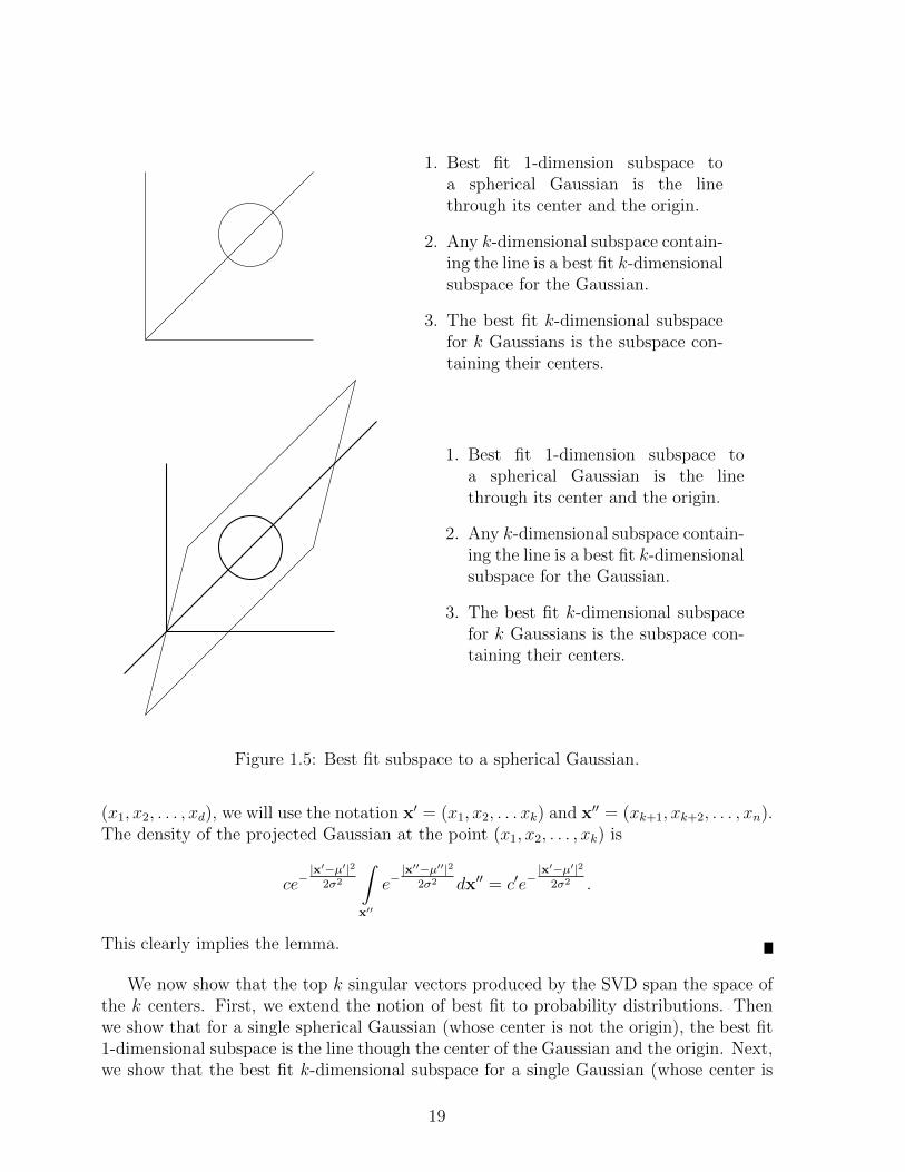
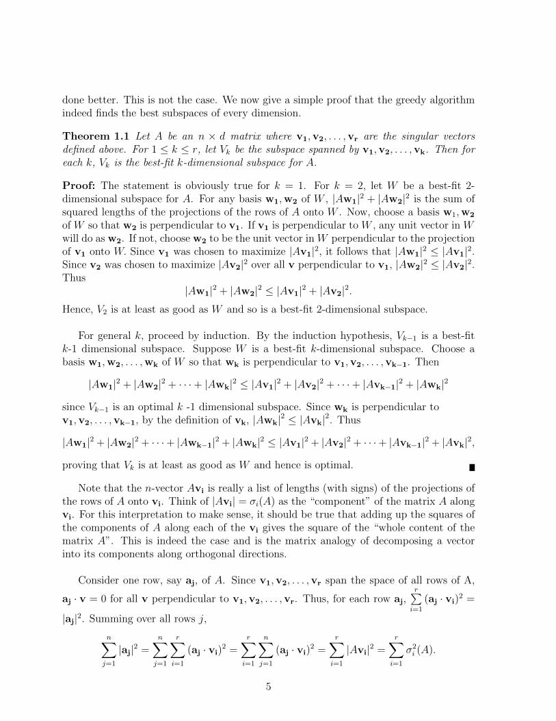
1. Best fit 1-dimension subspace toa spherical Gaussian is the linethrough its center and the origin.

2. Any k-dimensional subspace contain-ing the line is a best fit k-dimensionalsubspace for the Gaussian.

3. The best fit k-dimensional subspacefor k Gaussians is the subspace con-taining their centers.

Figure 1.5: Best fit subspace to a spherical Gaussian.

(x1, x2, . . . , xd), we will use the notation x′ = (x1, x2, . . . xk) and x′′ = (xk+1, xk+2, . . . , xn).The density of the projected Gaussian at the point (x1, x2, . . . , xk) is

ce−|x′−µ′|2

2σ2

∫x′′

e−|x′′−µ′′|2

2σ2 dx′′ = c′e−|x′−µ′|2

2σ2 .

This clearly implies the lemma.

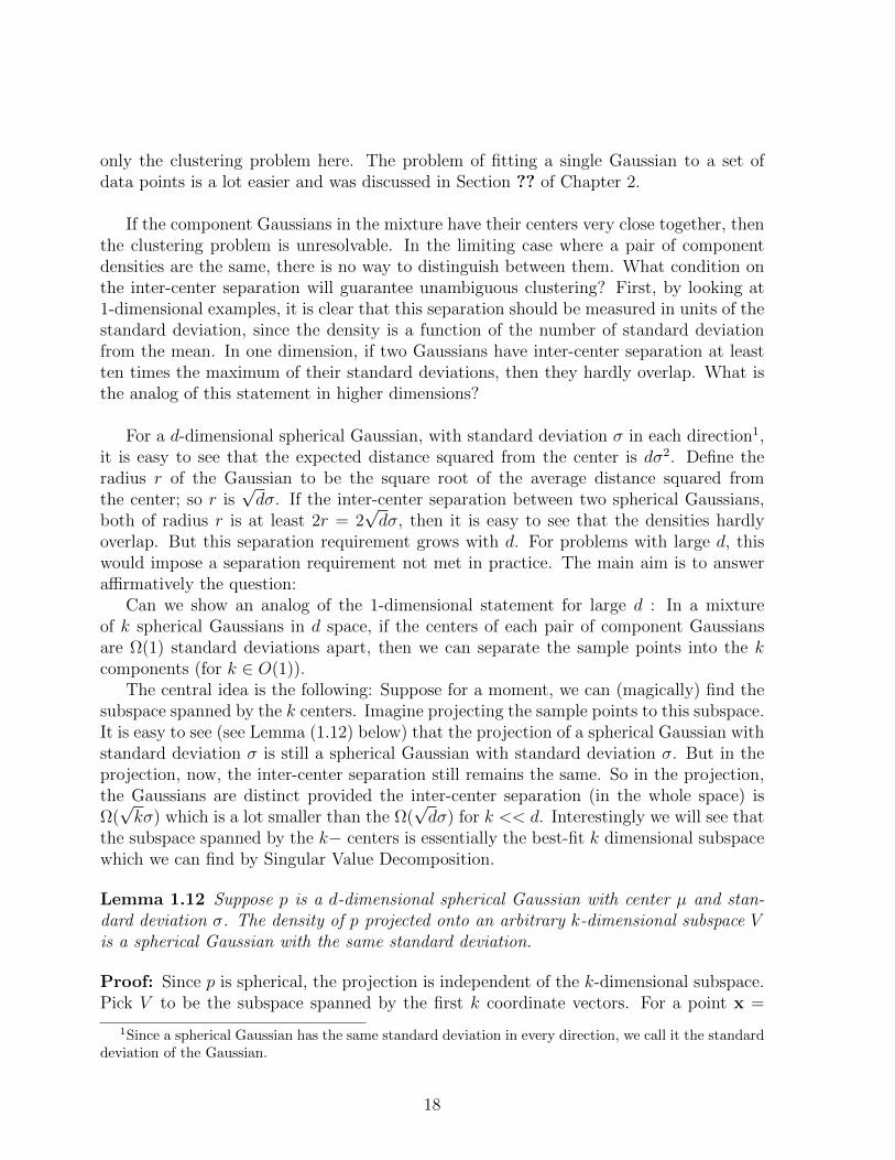
We now show that the top k singular vectors produced by the SVD span the space ofthe k centers. First, we extend the notion of best fit to probability distributions. Thenwe show that for a single spherical Gaussian (whose center is not the origin), the best fit1-dimensional subspace is the line though the center of the Gaussian and the origin. Next,we show that the best fit k-dimensional subspace for a single Gaussian (whose center is

19

not the origin) is any k-dimensional subspace containing the line through the Gaussian’scenter and the origin. Finally, for k spherical Gaussians, the best fit k-dimensional sub-space is the subspace containing their centers. Thus, the SVD finds the subspace thatcontains the centers.

Recall that for a set of points, the best-fit line is the line passing through the originwhich minimizes the sum of squared distances to the points. We extend this definition toprobability densities instead of a set of points.

Definition 4.1: If p is a probability density in d space, the best fit line for p is theline l passing through the origin that minimizes the expected squared (perpendicular)distance to the line, namely,

∫dist (x, l)2 p (x) dx.

Recall that a k-dimensional subspace is the best-fit subspace if the sum of squareddistances to it is minimized or equivalently, the sum of squared lengths of projections ontoit is maximized. This was defined for a set of points, but again it can be extended to adensity as above.

Definition 4.2: If p is a probability density in d-space and V is a subspace, then theexpected squared perpendicular distance of V to p, denoted f(V, p), is given by

f(V, p) =

∫dist2 (x, V ) p (x) dx,

where dist(x, V ) denotes the perpendicular distance from the point x to the subspace V .

For the uniform density on the unit circle centered at the origin, it is easy to see thatany line passing through the origin is a best fit line for the probability distribution.

Lemma 1.13 Let the probability density p be a spherical Gaussian with center µ 6= 0.The best fit 1-dimensional subspace is the line passing through µ and the origin.

Proof: For a randomly chosen x (according to p) and a fixed unit length vector v,

E[(vTx)2

]= E

[(vT (x− µ) + vTµ

)2]

= E[(

vT (x− µ))2

+ 2(vTµ

) (vT (x− µ)

)+(vTµ

)2]

= E[(

vT (x− µ))2]

+ 2(vTµ

)E[vT (x− µ)

]+(vTµ

)2

= E[(

vT (x− µ))2]

+(vTµ

)2

= σ2 +(vTµ

)2

20

since E[(

vT (x− µ))2]

is the variance in the direction v and E(vT (x− µ)

)= 0. The

lemma follows from the fact that the best fit line v is the one that maximizes(vTu

)2

which is maximized when v is aligned with the center µ.

Lemma 1.14 For a spherical Gaussian with center µ, a k-dimensional subspace is a bestfit subspace if and only if it contains µ.

Proof: By symmetry, every k-dimensional subspace through µ has the same sum ofdistances squared to the density. Now by the SVD procedure, we know that the best-fit k-dimensional subspace contains the best fit line, i.e., contains µ. Thus, the lemmafollows.

This immediately leads to the following theorem.

Theorem 1.15 If p is a mixture of k spherical Gaussians whose centers span a k-dimensional subspace, then the best fit k-dimensional subspace is the one containing thecenters.

Proof: Let p be the mixture w1p1+w2p2+· · ·+wkpk. Let V be any subspace of dimensionk or less. Then, the expected squared perpendicular distance of V to p is

f(V, p) =

∫dist2(x, V )p(x)dx

=k∑i=1

wi

∫dist2(x, V )pi(x)dx

≥k∑i=1

wi( distance squared of pi to its best fit k-dimensional subspace).

Choose V to be the space spanned by the centers of the densities pi. By Lemma ?? thelast inequality becomes an equality proving the theorem.

For an infinite set of points drawn according to the mixture, the k-dimensional SVDsubspace gives exactly the space of the centers. In reality, we have only a large numberof samples drawn according to the mixture. However, it is intuitively clear that as thenumber of samples increases, the set of sample points approximates the probability densityand so the SVD subspace of the sample is close to the space spanned by the centers. Thedetails of how close it gets as a function of the number of samples are technical and wedo not carry this out here.

21

1.5.3 An Application of SVD to a Discrete Optimization Problem

In the last example, SVD was used as a dimension reduction technique. It founda k-dimensional subspace (the space of centers) of a d-dimensional space and made theGaussian clustering problem easier by projecting the data to the subspace. Here, insteadof fitting a model to data, we have an optimization problem. Again applying dimensionreduction to the data makes the problem easier. The use of SVD to solve discrete op-timization problems is a relatively new subject with many applications. We start withan important NP-hard problem, the Maximum Cut Problem for a directed graph G(V,E).

The Maximum Cut Problem is to partition the node set V of a directed graph intotwo subsets S and S so that the number of edges from S to S is maximized. Let A bethe adjacency matrix of the graph. With each vertex i, associate an indicator variable xi.The variable xi will be set to 1 for i ∈ S and 0 for i ∈ S. The vector x = (x1, x2, . . . , xn)is unknown and we are trying to find it (or equivalently the cut), so as to maximize thenumber of edges across the cut. The number of edges across the cut is precisely∑

i,j

xi(1− xj)aij.

Thus, the Maximum Cut Problem can be posed as the optimization problem

Maximize∑i,j

xi(1− xj)aij subject to xi ∈ 0, 1.

In matrix notation, ∑i,j

xi(1− xj)aij = xTA(1− x),

where 1 denotes the vector of all 1’s . So, the problem can be restated as

Maximize xTA(1− x) subject to xi ∈ 0, 1. (1.1)

The SVD is used to solve this problem approximately by computing the SVD of A and

replacing A by Ak =k∑i=1

σiuiviT in (1.1) to get

Maximize xTAk(1− x) subject to xi ∈ 0, 1. (1.2)

Note that the matrix Ak is no longer a 0-1 adjacency matrix.

We will show that:

1. For each 0-1 vector x, xTAk(1− x) and xTA(1− x) differ by at most n2√k+1

. Thus,

the maxima in (1.1) and (1.2) differ by at most this amount.

2. A near optimal x for (1.2) can be found by exploiting the low rank of Ak, which byItem 1 is near optimal for (1.1) where near optimal means with additive error of atmost n2

√k+1

.

22

First, we prove Item 1. Since x and 1− x are 0-1 n-vectors, each has length at most√n. By the definition of the 2-norm, |(A − Ak)(1 − x)| ≤

√n||A − Ak||2. Now since

xT (A− Ak)(1− x) is the dot product of the vector x with the vector (A− Ak)(1− x),

|xT (A− Ak)(1− x)| ≤ n||A− Ak||2.

By Lemma 1.8, ||A− Ak||2 = σk+1(A). The inequalities,

(k + 1)σ2k+1 ≤ σ2

1 + σ22 + · · ·σ2

k+1 ≤ ||A||2F =∑i,j

a2ij ≤ n2

imply that σ2k+1 ≤ n2

k+1and hence ||A− Ak||2 ≤ n√

k+1proving Item 1.

Next we focus on Item 2. It is instructive to look at the special case when k=1 and Ais approximated by the rank one matrix A1. An even more special case when the left andright singular vectors u and v are required to be identical is already NP-hard to solve ex-actly because it subsumes the problem of whether for a set of n integers, a1, a2, . . . , an,there is a partition into two subsets whose sums are equal. So, we look for algorithmsthat solve the Maximum Cut Problem approximately.

For Item 2, we want to maximize∑k

i=1 σi(xTui)(vi

T (1 − x)) over 0-1 vectors x. Apiece of notation will be useful. For any S ⊆ 1, 2, . . . n, write ui(S) for the sum ofcoordinates of the vector ui corresponding to elements in the set S and also for vi. Thatis, ui(S) =

∑j∈S

uij. We will maximize∑k

i=1 σiui(S)vi(S) using dynamic programming.

For a subset S of 1, 2, . . . , n, define the 2k-dimensional vector w(S) = (u1(S),v1(S),u2(S),v2(S), . . . ,uk(S),vk(S)).If we had the list of all such vectors, we could find

∑ki=1 σiui(S)vi(S) for each of them

and take the maximum. There are 2n subsets S, but several S could have the samew(S) and in that case it suffices to list just one of them. Round each coordinate ofeach ui to the nearest integer multiple of 1

nk2. Call the rounded vector ui. Similarly ob-

tain vi. Let w(S) denote the vector (u1(S), v1(S), u2(S), v2(S), . . . , uk(S), vk(S)). Wewill construct a list of all possible values of the vector w(S). [Again, if several differ-ent S ’s lead to the same vector w(S), we will keep only one copy on the list.] Thelist will be constructed by Dynamic Programming. For the recursive step of DynamicProgramming, assume we already have a list of all such vectors for S ⊆ 1, 2, . . . , iand wish to construct the list for S ⊆ 1, 2, . . . , i + 1. Each S ⊆ 1, 2, . . . , i leads totwo possible S ′ ⊆ 1, 2, . . . , i + 1, namely, S and S ∪ i + 1. In the first case, thevector w(S ′) = (u1(S) + u1,i+1, v1(S), u2(S) + u2,i+1, v2(S), . . . , ...). In the second case,w(S ′) = (u1(S), v1(S) + v1,i+1, u2(S), v2(S) + v2,i+1, . . . , ...). We put in these two vectorsfor each vector in the previous list. Then, crucially, we prune - i.e., eliminate duplicates.

Assume that k is constant. Now, we show that the error is at most n2√k+1

as claimed.

Since ui,vi are unit length vectors, |ui(S)|, |vi(S)| ≤√n. Also |ui(S)−ui(S)| ≤ n

nk2= 1

k2

and similarly for vi. To bound the error, we use an elementary fact: if a, b are reals with|a|, |b| ≤M and we estimate a by a′ and b by b′ so that |a− a′|, |b− b′| ≤ δ ≤M , then

|ab− a′b′| = |a(b− b′) + b′(a− a′)| ≤ |a||b− b′|+ (|b|+ |b− b′|)|a− a′| ≤ 3Mδ.

23

Using this, we get that∣∣∣∣∣k∑i=1

σiui(S)vi(S) −k∑i=1

σiui(S)vi(S)

∣∣∣∣∣ ≤ 3kσ1

√n/k2 ≤ 3n3/2/k,

and this meets the claimed error bound.Next, we show that the running time is polynomially bounded. |ui(S)|, |vi(S)| ≤ 2

√n.

Since ui(S), vi(S) are all integer multiples of 1/(nk2), there are at most 2/√nk2 possible

values of ui(S), vi(S) from which it follows that the list of w(S) never gets larger than(1/√nk2)2k which for fixed k is polynomially bounded.

We summarize what we have accomplished.

Theorem 1.16 Given a directed graph G(V,E), a cut of size at least the maximum cut

minus O(n2√k

)can be computed in polynomial time n for any fixed k.

It would be quite a surprise to have an algorithm that actually achieves the sameaccuracy in time polynomial in n and k because this would give an exact max cut inpolynomial time.

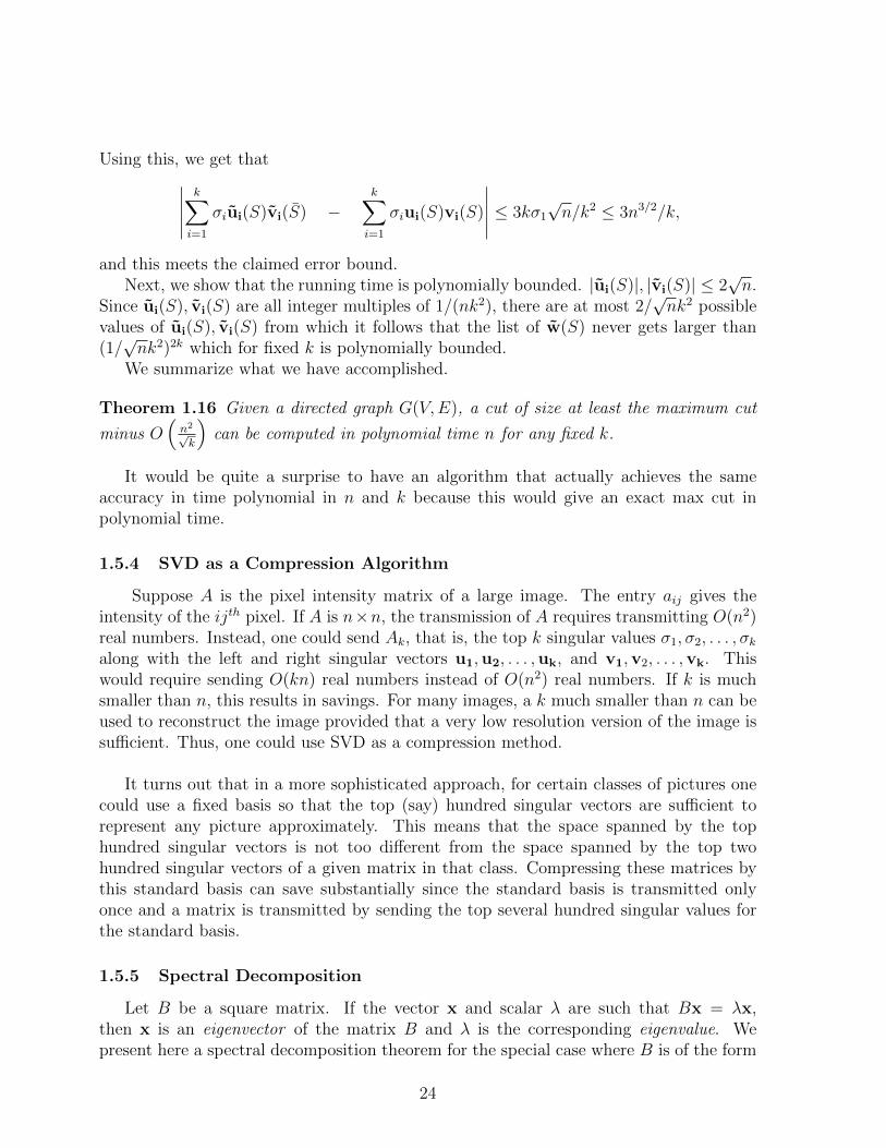
1.5.4 SVD as a Compression Algorithm

Suppose A is the pixel intensity matrix of a large image. The entry aij gives theintensity of the ijth pixel. If A is n×n, the transmission of A requires transmitting O(n2)real numbers. Instead, one could send Ak, that is, the top k singular values σ1, σ2, . . . , σkalong with the left and right singular vectors u1,u2, . . . ,uk, and v1,v2, . . . ,vk. Thiswould require sending O(kn) real numbers instead of O(n2) real numbers. If k is muchsmaller than n, this results in savings. For many images, a k much smaller than n can beused to reconstruct the image provided that a very low resolution version of the image issufficient. Thus, one could use SVD as a compression method.

It turns out that in a more sophisticated approach, for certain classes of pictures onecould use a fixed basis so that the top (say) hundred singular vectors are sufficient torepresent any picture approximately. This means that the space spanned by the tophundred singular vectors is not too different from the space spanned by the top twohundred singular vectors of a given matrix in that class. Compressing these matrices bythis standard basis can save substantially since the standard basis is transmitted onlyonce and a matrix is transmitted by sending the top several hundred singular values forthe standard basis.

1.5.5 Spectral Decomposition

Let B be a square matrix. If the vector x and scalar λ are such that Bx = λx,then x is an eigenvector of the matrix B and λ is the corresponding eigenvalue. Wepresent here a spectral decomposition theorem for the special case where B is of the form

24

B = AAT for some (possibly rectangular) matrix A. If A is a real valued matrix, thenB is symmetric and positive definite. That is, xTBx > 0 for all nonzero vectors x. Thespectral decomposition theorem holds more generally and the interested reader shouldconsult a linear algebra book.

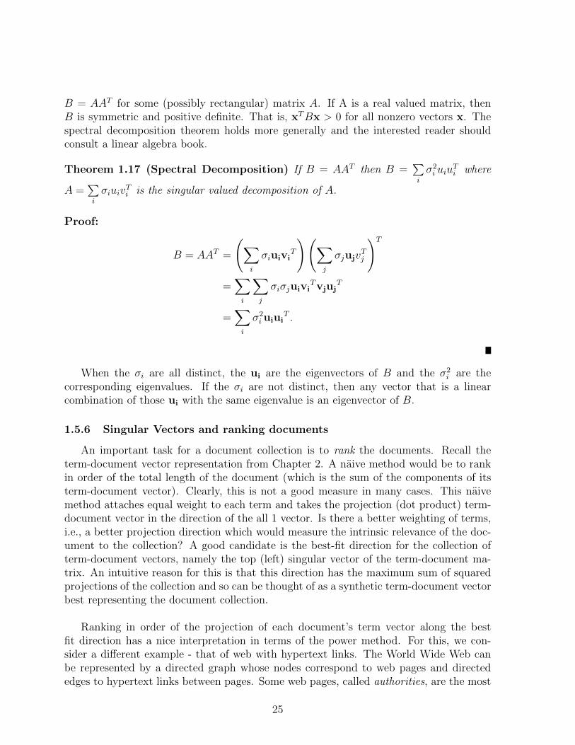
Theorem 1.17 (Spectral Decomposition) If B = AAT then B =∑i

σ2i uiu

Ti where

A =∑i

σiuivTi is the singular valued decomposition of A.

Proof:

B = AAT =

(∑i

σiuiviT

)(∑j

σjujvTj

)T

=∑i

∑j

σiσjuiviTvjuj

T

=∑i

σ2i uiui

T .

When the σi are all distinct, the ui are the eigenvectors of B and the σ2i are the

corresponding eigenvalues. If the σi are not distinct, then any vector that is a linearcombination of those ui with the same eigenvalue is an eigenvector of B.

1.5.6 Singular Vectors and ranking documents

An important task for a document collection is to rank the documents. Recall theterm-document vector representation from Chapter 2. A naive method would be to rankin order of the total length of the document (which is the sum of the components of itsterm-document vector). Clearly, this is not a good measure in many cases. This naivemethod attaches equal weight to each term and takes the projection (dot product) term-document vector in the direction of the all 1 vector. Is there a better weighting of terms,i.e., a better projection direction which would measure the intrinsic relevance of the doc-ument to the collection? A good candidate is the best-fit direction for the collection ofterm-document vectors, namely the top (left) singular vector of the term-document ma-trix. An intuitive reason for this is that this direction has the maximum sum of squaredprojections of the collection and so can be thought of as a synthetic term-document vectorbest representing the document collection.

Ranking in order of the projection of each document’s term vector along the bestfit direction has a nice interpretation in terms of the power method. For this, we con-sider a different example - that of web with hypertext links. The World Wide Web canbe represented by a directed graph whose nodes correspond to web pages and directededges to hypertext links between pages. Some web pages, called authorities, are the most

25

prominent sources for information on a given topic. Other pages called hubs, are onesthat identify the authorities on a topic. Authority pages are pointed to by many hubpages and hub pages point to many authorities. One is led to what seems like a circulardefinition: a hub is a page that points to many authorities and an authority is a pagethat is pointed to by many hubs.

One would like to assign hub weights and authority weights to each node of the web.If there are n nodes, the hub weights form a n-dimensional vector u and the authorityweights form a n-dimensional vector v. Suppose A is the adjacency matrix representingthe directed graph : aij is 1 if there is a hypertext link from page i to page j and 0otherwise. Given hub vector u, the authority vector v could be computed by the formula

vj =d∑i=1

uiaij

since the right hand side is the sum of the hub weights of all the nodes that point to nodej. In matrix terms,

v = ATu.

Similarly, given an authority vector v, the hub vector u could be computed by u = Av.Of course, at the start, we have neither vector. But the above suggests a power iteration.Start with any v. Set u = Av; then set v = ATu and repeat the process. We knowfrom the power method that this converges to the left and right singular vectors. Soafter sufficiently many iterations, we may use the left vector u as hub weights vector andproject each column of A onto this direction and rank columns (authorities) in order ofthis projection. But the projections just form the vector ATu which equals v. So we canjust rank by order of vj.

This is the basis of an algorithm called the HITS algorithm which was one of the earlyproposals for ranking web pages.

A different ranking called page rank is widely used. It is based on a random walk onthe grap described above. (We will study Random Walks in detail in Chapter 5 and thereader may postpone reading this application until then.)

A random walk on the web goes from web page i to a randomly chosen neighbor of it.so if pij is the probability of going from i to j, then pij is just 1/ (number of hypertext linksfrom i). Represent the pij in a matrix P . This matrix is called the transition probabilitymatrix of the random walk. Represent the probabilities of being in each state at time tby the components of a row vector p (t). The probability of being in state j at time t isgiven by the equation

pj (t) =∑i

pi (t− 1) pij.

Thenp (t) = p (t− 1)P

26

and thusp (t) = p (0)P t.

The probability vector p (t) is computed by computing P to the power t. It turns out thatunder some conditions, the random walk has a steady state probability vector that we canthink of as p (∞). It has turned out to be very useful to rank pages in decreasing orderof pj (∞) in essence saying that the web pages with the highest steady state probabilitiesare the most important.

In the above explanation, the random walk goes from page i to one of the web pagespointed to by i, picked uniformly at random. Modern technics for ranking pages are morecomplex. A more sophisticated random walk is used for several reasons. First, a webpage might not contain any links and thus there is nowhere for the walk to go. Second,a page that has no in links will never be reached. Even if every node had at least onein link and one out link, the graph might not be strongly connected and the walk wouldeventually end up in some strongly connected component of the graph. Another difficultyoccurs when the graph is periodic, that is, the greatest common divisor of all cycle lengthsof the graph is greater than one. In this case, the random walk does not converge to astationary probability distribution but rather oscillates between some set of probabilitydistributions. We will consider this topic further in Chapter 5.

1.6 Bibliographic Notes

Singular value decomposition is fundamental to numerical analysis and linear algebra.There are many texts on these subjects and the interested reader may want to study these.A good reference is [?]. The material on clustering a mixture of Gaussians in Section 1.5.2is from [?]. Modeling data with a mixture of Gaussians is a standard tool in statistics.Several well-known heuristics like the expectation-minimization algorithm are used tolearn (fit) the mixture model to data. Recently, in theoretical computer science, therehas been modest progress on provable polynomial-time algorithms for learning mixtures.Some references are [?], [?], [?], [?]. The application to the discrete optimization problemis from [?]. The section on ranking documents/webpages is from two influential papers,one on hubs and authorities by Jon Kleinberg [?] and the other on pagerank by Page,Brin, Motwani and Winograd [?].

27

1.7 Exercises

Exercise 1.1 (Best fit functions versus best least squares fit) In many experimentsone collects the value of a parameter at various instances of time. Let yi be the value ofthe parameter y at time xi. Suppose we wish to construct the best linear approximationto the data in the sense that we wish to minimize the mean square error. Here error ismeasured vertically rather than perpendicular to the line. Develop formulas for m and b tominimize the mean square error of the points (xi, yi) |1 ≤ i ≤ n to the line y = mx+ b.

Exercise 1.2 Given five observed parameters, height, weight, age, income, and bloodpressure of n people, how would one find the best least squares fit subspace of the form

a1 (height) + a2 (weight) + a3 (age) + a4 (income) + a5 (blood pressure) = 0

Here a1, a2, . . . , a5 are the unknown parameters. If there is a good best fit 4-dimensionalsubspace, then one can think of the points as lying close to a 4-dimensional sheet ratherthan points lying in 5-dimensions. Why is it better to use the perpendicular distance to thesubspace rather than vertical distance where vertical distance to the subspace is measuredalong the coordinate axis corresponding to one of the unknowns?

Exercise 1.3 What is the best fit line for each of the following set of points?

1. (0, 1) , (1, 0)

2. (0, 1) , (2, 0)

3. The rows of the matrix 17 4−2 2611 7

Solution: (1) and (2) are easy to do from scratch. (1) y = x and (2) y = 2x. For(3), there is no simple method. We will describe a general method later and this can

be applied. But the best fit line is v1 = 1√5

(12

). FIX Convince yourself that this is

correct.

Exercise 1.4 Let A be a square n × n matrix whose rows are orthonormal. Prove thatthe columns of A are orthonormal.

Solution: Since the rows of A are orthonormal AAT = I and hence ATAAT = AT . SinceAT is nonsingular it has an inverse

(AT)−1

. Thus ATAAT(AT)−1

= AT(AT)−1

implyingthat ATA = I, i.e., the columns of A are orthonormal.

28

Exercise 1.5 Suppose A is a n×n matrix with block diagonal structure with k equal sizeblocks where all entries of the ith block are ai with a1 > a2 > · · · > ak > 0. Show that Ahas exactly k nonzero singular vectors v1,v2, . . . ,vk where vi has the value ( k

n)1/2 in the

coordinates corresponding to the ith block and 0 elsewhere. In other words, the singularvectors exactly identify the blocks of the diagonal. What happens if a1 = a2 = · · · = ak?In the case where the ai are equal, what is the structure of the set of all possible singularvectors?Hint: By symmetry, the top singular vector’s components must be constant in each block.

Exercise 1.6 Prove that the left singular vectors of A are the right singular vectors ofAT .

Solution: A = UDV T , thus AT = V DUT .

Exercise 1.7 Interpret the right and left singular vectors for the document term matrix.

Solution: The first right singular vector is a synthetic document that best matches thecollection of documents. The first left singular vector is a synthetic word that best matchesthe collection of terms appearing in the documents.

Exercise 1.8 Verify that the sum of rank one matricesr∑i=1

σiuiviT can be written as

UDV T , where the ui are the columns of U and vi are the columns of V . To do this, firstverify that for any two matrices P and Q, we have

PQ =∑i

piqiT

where pi is the ith column of P and qi is the ith column of Q.

Exercise 1.9

1. Show that the rank of A is r where r is the miminum i such that arg maxv⊥v1,v2,...,vi|v|=1

|A v| = 0.

2. Show that∣∣uT1A∣∣ = max

|u|=1

∣∣uTA∣∣ = σ1.

Hint: Use SVD.

Exercise 1.10 If σ1, σ2, . . . , σr are the singular values of A and v1,v2, . . . ,vr are thecorresponding right singular vectors, show that

1. ATA =r∑i=1

σ2i vivi

T

29

2. v1,v2, . . .vr are eigenvectors ofATA.

3. Assuming that the set of eigenvectors of a matrix is unique, conclude that the set ofsingular values of the matrix is unique.

See the appendix for the definition of eigenvectors.

Exercise 1.11 Let A be a matrix. Given an algorithm for finding

v1 = arg max|v|=1

|Av|

describe an algorithm to find the SVD of A.

Exercise 1.12 Compute the singular valued decomposition of the matrix

A =

(1 23 4

)Exercise 1.13 Write a program to implement the power method for computing the firstsingular vector of a matrix. Apply your program to the matrix

A =

1 2 3 · · · 9 102 3 4 · · · 10 0...

......

...9 10 0 · · · 0 010 0 0 · · · 0 0

Exercise 1.14 Modify the power method to find the first four singular vectors of a matrixA as follows. Randomly select four vectors and find an orthonormal basis for the spacespanned by the four vectors. Then multiple each of the basis vectors times A and find anew orthonormal basis for the space spanned by the resulting four vectors. Apply yourmethod to find the first four singular vectors of matrix A of Exercise 1.13

Exercise 1.15 Let A be a real valued matrix. Prove that B = AAT is positive definite.

Exercise 1.16 Prove that the eigenvalues of a symmetric real valued matrix are real.

Exercise 1.17 Suppose A is a square invertible matrix and the SVD of A is A =∑i

σiuivTi .

Prove that the inverse of A is∑i

1σiviu

Ti .

Exercise 1.18 Suppose A is square, but not necessarily invertible and has SVD A =r∑i=1

σiuivTi . Let B =

r∑i=1

1σiviu

Ti . Show that Bx = x for all x in the span of the right

singular vectors of A. For this reason B is sometimes called the pseudo inverse of A andcan play the role of A−1 in many applications.

30

Exercise 1.19

1. For any matrix A, show that σk ≤ ||A||F√k

.

2. Prove that there exists a matrix B of rank at most k such that ||A−B||2 ≤ ||A||F√k

.

3. Can the 2-norm on the left hand side in (b) be replaced by Frobenius norm?

Exercise 1.20 Suppose an n × d matrix A is given and you are allowed to preprocessA. Then you are given a number of d-dimensional vectors x1,x2, . . . ,xm and for each ofthese vectors you must find the vector Axi approximately, in the sense that you must find avector ui satisfying |ui−Axi| ≤ ε||A||F |xi|. Here ε >0 is a given error bound. Describean algorithm that accomplishes this in time O

(d+nε2

)per xi not counting the preprocessing

time.

Exercise 1.21 (Constrained Least Squares Problem using SVD) Given A, b,and m, use the SVD algorithm to find a vector x with |x| < m minimizing |Ax−b|. Thisproblem is a learning exercise for the advanced student. For hints/solution consult Goluband van Loan, Chapter 12.

Exercise 1.22 (Document-Term Matrices): Suppose we have a m×n document-termmatrix where each row corresponds to a document where the rows have been normalizedto length one. Define the “similarity” between two such documents by their dot product.

1. Consider a “synthetic” document whose sum of squared similarities with all docu-ments in the matrix is as high as possible. What is this synthetic document and howwould you find it?

2. How does the synthetic document in (1) differ from the center of gravity?

3. Building on (1), given a positive integer k, find a set of k synthetic documents suchthat the sum of squares of the mk similarities between each document in the matrixand each synthetic document is maximized. To avoid the trivial solution of selectingk copies of the document in (1), require the k synthetic documents to be orthogonalto each other. Relate these synthetic documents to singular vectors.

4. Suppose that the documents can be partitioned into k subsets (often called clusters),where documents in the same cluster are similar and documents in different clustersare not very similar. Consider the computational problem of isolating the clusters.This is a hard problem in general. But assume that the terms can also be partitionedinto k clusters so that for i 6= j, no term in the ith cluster occurs in a documentin the jth cluster. If we knew the clusters and arranged the rows and columns inthem to be contiguous, then the matrix would be a block-diagonal matrix. Of course

31

the clusters are not known. By a “block” of the document-term matrix, we meana submatrix with rows corresponding to the ithcluster of documents and columnscorresponding to the ithcluster of terms . We can also partition any n vector intoblocks. Show that any right singular vector of the matrix must have the propertythat each of its blocks is a right singular vector of the corresponding block of thedocument-term matrix.

5. Suppose now that the singular values of all the blocks are distinct (also across blocks).Show how to solve the clustering problem.

Hint: (4) Use the fact that the right singular vectors must be eigenvectors of ATA. Showthat ATA is also block-diagonal and use properties of eigenvectors.

Solution: (1)(2)(3): It is obvious that ATA is block diagonal. We claim that for any block-diagonalsymmetric matrix B, each eigenvector must be composed of eigenvectors of blocks. Tosee this, just note that since for an eigenvector v of B, Bv is λv for a real λ, for a blockBi of B, Biv is also λ times the corresponding block of v .(4): By the above, it is easy to see that each eigenvector of ATA has nonzero entries injust one block.(e)

Exercise 1.23 Generate a number of samples according to a mixture of 1-dimensionalGaussians. See what happens as the centers get closer. Alternatively, see what happenswhen the centers are fixed and the standard deviation is increased.

Exercise 1.24 Show that maximizing xTuuT (1 − x) subject to xi ∈ 0, 1 is equivalentto partitioning the coordinates of u into two subsets where the sum of the elements in bothsubsets are equal.

Solution: xTuuT (1−x) can be written as the product of two scalars(xTu

) (uT (1− x)

).

The first scalar is the sum of the coordinates of u corresponding to the subset S and thesecond scalar is the sum of the complementary coordinates of u. To maximize the product,one partitions the coordinates of u so that the two sums are as equally as possible. Giventhe subset determined by the maximization, check if xTu = uT (1− x).

Exercise 1.25 Read in a photo and convert to a matrix. Perform a singular value decom-position of the matrix. Reconstruct the photo using only 10%, 25%, 50% of the singularvalues.

1. Print the reconstructed photo. How good is the quality of the reconstructed photo?

2. What percent of the Forbenius norm is captured in each case?

32

Hint: If you use Matlab, the command to read a photo is imread. The types of files thatcan be read are given by imformats. To print the file use imwrite. Print using jpeg format.To access the file afterwards you may need to add the file extension .jpg. The commandimread will read the file in uint8 and you will need to convert to double for the SVD code.Afterwards you will need to convert back to uint8 to write the file. If the photo is a colorphoto you will get three matrices for the three colors used.

Exercise 1.26 Find a collection of something such as photgraphs, drawings, or chartsand try the SVD compression technique on it. How well does the reconstruction work?

Exercise 1.27 Create a set of 100, 100×100 matrices of random numbers between 0 and1 such that each entry is highly correlated with the adjacency entries. Find the SVD ofA. What fraction of the Frobenius norm of A is captured by the top 100 singular vectors?How many singular vectors are required to capture 95% of the Frobenius norm?

Exercise 1.28 Create a 100 × 100 matrix A of random numbers between 0 and 1 suchthat each entry is highly correlated with the adjacency entries and find the first 100 vectorsfor a single basis that is reasonably good for all 100 matrices. How does one do this? Whatfraction of the Frobenius norm of a new matrix is captured by the basis?

Solution: If v1,v2, · · · ,v100 is the basis, then A = Av1v1T + Av2v2

T + · · · .

Exercise 1.29 Show that the running time for the maximum cut algorithm in Section ??can be carried out in time O(n3 + poly(n)kk), where poly is some polynomial.

Exercise 1.30 Let x1, x2, . . . , xn be n points in d-dimensional space and let X be then×d matrix whose rows are the n points. Suppose we know only the matrix D of pairwisedistances between points and not the coordinates of the points themselves. The xij are notunique since any translation, rotation, or reflection of the coordinate system leaves thedistances invariant. Fix the origin of the coordinate system so that the centroid of the setof points is at the origin.

1. Show that the elements of XTX are given by

xTi xj = −1

2

[d2ij −

1

n

n∑j=1

d2ij −

1

n

n∑i=1

d2ij +

1

n

n∑i=1

n∑j=1

d2ij

].

2. Describe an algorithm for determining the matrix X whose rows are the xi.

Solution: (1) Since the centroid of the set of points is at the origin of the coordinateaxes,

∑ni=1 xij = 0. Write

d2ij = (xi − xj)T (xi − xj) = xTi xi + xTj xj − 2xTi xj (1.3)

33

Then1

n

n∑i=1

d2ij =

1

n

n∑i=1

xTi xi + xTj xj (1.4)

Since 1n

∑ni=1 x

Tj xj = xTj xj and 1

n

(∑ni=1 x

Ti

)xj = 0.

Similarly1

n

n∑j=1

d2ij =

1

n

n∑j=1

xTj xj + xTi xi (1.5)

Summing (1.4) over j gives

1

n

n∑j=1

n∑i=1

d2ij =

n∑i=1

xTi xi +n∑j=1

xTj xj = 2n∑i=1

xTi xi (1.6)

Rearranging (1.3) and substituting for xTi xi and xTj xj from (1.3) and (1.4) yields

xTi xj = −1

2

(d2ij − xTi xi − xTj xj

)= −1

2

(d2ij −

1

n

n∑j=1

d2ij −

1

n

n∑i=1

d2ij +

2

n

n∑i=1

xTi xi

)

Finally substituting (1.6) yields

xTi xj = −1

2

(d2ij − xTi xi − xTj xj

)= −1

2

(d2ij −

1

n

n∑j=1

d2ij −

1

n

n∑i=1

d2ij +

1

n2

n∑j=1

n∑i=1

d2ij

)

Note that is D is the matrix of pairwise squared distances, then 1n

∑nk=1 d

2ij,

1n

∑ni=1 d

2ij,

and 1n2

∑ni=1

∑nj=1 d

2ij are the averages of the square of the elements of the ith row, the

square of the elements of the jth column and all squared distances respectively.(2) Having constructed XTX we can use an eigenvalue decomposition to determine thecoordinate matrix X. Clearly XTX is symmetric and if the distances come from a set ofn points in a d-dimensional space XTX will be positive definite and of rank d. Thus wecan decompose XTX asXTX = V TσV where the first d eigenvalues are positive and theremainder are zero. Since the XTX = V Tσ

12σ

12V and thus the coordinates are given by

X = V Tσ12

Exercise 1.31

1. Consider the pairwise distance matrix for twenty US cities given below. Use thealgorithm of Exercise 2 to place the cities on a map of the US.

2. Suppose you had airline distances for 50 cities around the world. Could you usethese distances to construct a world map?

34

B B C D D H L M M MO U H A E O A E I IS F I L N U M A M

Boston - 400 851 1551 1769 1605 2596 1137 1255 1123Buffalo 400 - 454 1198 1370 1286 2198 803 1181 731Chicago 851 454 - 803 920 940 1745 482 1188 355Dallas 1551 1198 803 - 663 225 1240 420 1111 862Denver 1769 1370 920 663 - 879 831 879 1726 700Houston 1605 1286 940 225 879 - 1374 484 968 1056Los Angeles 2596 2198 1745 1240 831 1374 - 1603 2339 1524Memphis 1137 803 482 420 879 484 1603 - 872 699Miami 1255 1181 1188 1111 1726 968 2339 872 - 1511Minneapolis 1123 731 355 862 700 1056 1524 699 1511 -New York 188 292 713 1374 1631 1420 2451 957 1092 1018Omaha 1282 883 432 586 488 794 1315 529 1397 290Philadelphia 271 279 666 1299 1579 1341 2394 881 1019 985Phoenix 2300 1906 1453 887 586 1017 357 1263 1982 1280Pittsburgh 483 178 410 1070 1320 1137 2136 660 1010 743Saint Louis 1038 662 262 547 796 679 1589 240 1061 466Salt Lake City 2099 1699 1260 999 371 1200 579 1250 2089 987San Francisco 2699 2300 1858 1483 949 1645 347 1802 2594 1584Seattle 2493 2117 1737 1681 1021 1891 959 1867 2734 1395Washington D.C. 393 292 597 1185 1494 1220 2300 765 923 934

35

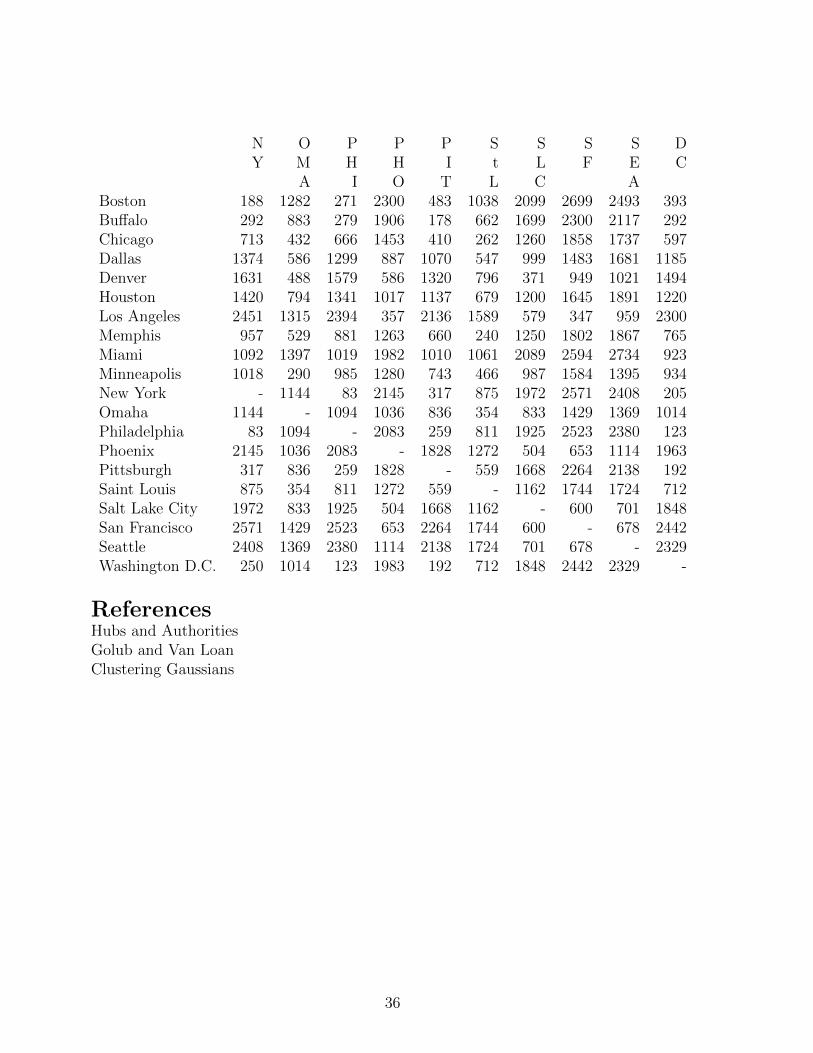
N O P P P S S S S DY M H H I t L F E C

A I O T L C ABoston 188 1282 271 2300 483 1038 2099 2699 2493 393Buffalo 292 883 279 1906 178 662 1699 2300 2117 292Chicago 713 432 666 1453 410 262 1260 1858 1737 597Dallas 1374 586 1299 887 1070 547 999 1483 1681 1185Denver 1631 488 1579 586 1320 796 371 949 1021 1494Houston 1420 794 1341 1017 1137 679 1200 1645 1891 1220Los Angeles 2451 1315 2394 357 2136 1589 579 347 959 2300Memphis 957 529 881 1263 660 240 1250 1802 1867 765Miami 1092 1397 1019 1982 1010 1061 2089 2594 2734 923Minneapolis 1018 290 985 1280 743 466 987 1584 1395 934New York - 1144 83 2145 317 875 1972 2571 2408 205Omaha 1144 - 1094 1036 836 354 833 1429 1369 1014Philadelphia 83 1094 - 2083 259 811 1925 2523 2380 123Phoenix 2145 1036 2083 - 1828 1272 504 653 1114 1963Pittsburgh 317 836 259 1828 - 559 1668 2264 2138 192Saint Louis 875 354 811 1272 559 - 1162 1744 1724 712Salt Lake City 1972 833 1925 504 1668 1162 - 600 701 1848San Francisco 2571 1429 2523 653 2264 1744 600 - 678 2442Seattle 2408 1369 2380 1114 2138 1724 701 678 - 2329Washington D.C. 250 1014 123 1983 192 712 1848 2442 2329 -

ReferencesHubs and AuthoritiesGolub and Van LoanClustering Gaussians

36