sinisa edinburgh

8/8/2019 Sinisa Edinburgh

http://slidepdf.com/reader/full/sinisa-edinburgh 1/10

9TH INTERNATIONAL SYMPOSIUM ON FLOW VISUALISATION, 2000

FLOW AROUND A THREE-DIMENSIONAL BLUFFBODY

S. Krajnovic 1 and L. Davidson2

Keywords: Large eddy simulation, bluff body, isosurface of Q

ABSTRACT

Large Eddy Simulation (LES) is used to compute the flow around a sharp-edged surface-mounted cube.Different visualization techniques were used, and the results of these are presented. Since Large Eddy

Simulation is a time-dependent three-dimensional numerical technique, it allows visualization that is unat-

tainable in RANS (Reynolds Averaged Navier Stokes) methods or experiments.

1 INTRODUCTION

Large Eddy Simulation is a numerical method that results in a three-dimensional time-dependent

solution. With the increases in computer power in the last ten years, this technique has grown

rapidly and is used in high Reynolds number flows and more complex geometries. While the

technique is intended for accurate predictions of statistics, a qualitative picture of instantaneous

flow can also be obtained.One area of application for LES is the wake behind a three-dimensional bluff body. The

physics of such a wake is not possible to predict with RANS methods because of the unsteady

nature of wakes. These unsteadiness can easily be captured using the LES technique as is shown

in this work. A movie can be made using the instantaneous data obtained from LES, making it

possible to study the flow in detail.

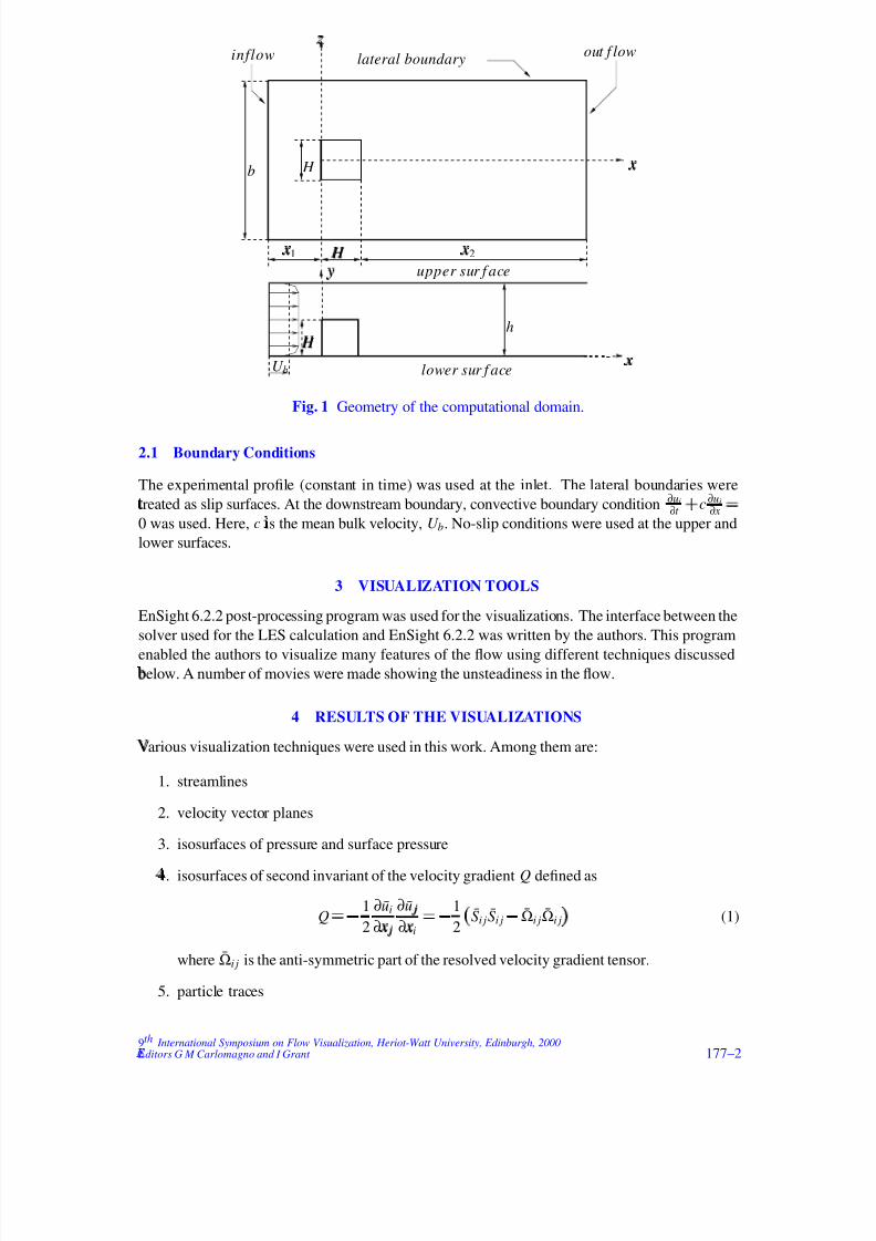
2 COMPUTATIONAL DETAILS

The Reynolds number was Re

U b H ν

40000 based on the incoming mean bulk velocity,

U b, and the obstacle height, H . The cube is located between x

0 and x

1, and the channel

height is h

2 H (see Fig. 1). A computational domain with an upstream length of x1

H

3and a downstream length of x2 H 6 was used, while the span-wise width was set to b H 7.

Even though the geometry of the flow configuration is rather simple, the flow is physically quite

complex, with multiple separation regions and vortices. A mesh of 82¢

50¢

66 nodes was used.

Near the walls of the cube, y ·

min

3

7, while, on the top of the cube, y·

min

5

2. The time step

was set to 0.02, which gave a maximum CFL number of approximately 2.

Author(s): 1 Dept. of Thermo and Fluid Dynamics, Chalmers University of Technology, SE-412 96 Göteborg,

Sweden2 Dept. of Thermo and Fluid Dynamics, Chalmers University of Technology, SE-412 96 Göteborg,

Sweden

Corresponding author: S. Krajnovi´ c

Paper number 177 177–1



b

h H

¡

H

H ¡

U b x

¢

x¢

y£

z¤

x¢

1 x¢

2

inflow out f lowlateral boundary

upper sur f ace

lower sur f ace

Fig. 1 Geometry of the computational domain.

2.1 Boundary Conditions

The experimental profile (constant in time) was used at the inlet. The lateral boundaries were

treated¥

as slip surfaces. At the downstream boundary, convective boundary condition ∂ui

∂t ¦

c∂ui

∂ x §

0 was used. Here, c is¨

the mean bulk velocity, U b. No-slip conditions were used at the upper and

lower surfaces.

3 VISUALIZATION TOOLS

EnSight 6.2.2 post-processing program was used for the visualizations. The interface between the

solver used for the LES calculation and EnSight 6.2.2 was written by the authors. This program

enabled the authors to visualize many features of the flow using different techniques discussedbelo

©

w. A number of movies were made showing the unsteadiness in the flow.

4 RESULTS OF THE VISUALIZATIONS

V

arious visualization techniques were used in this work. Among them are:

1. streamlines

2. velocity vector planes

3. isosurfaces of pressure and surface pressure

4.

isosurfaces of second invariant of the velocity gradient Q defined as

Q

1

2

∂ui

∂ x¢

j

∂u j

∂ x¢

i

1

2

Si jSi j

Ωi jΩi j

(1)

where Ωi j is the anti-symmetric part of the resolved velocity gradient tensor.

5. particle traces

9th International Symposium on Flow Visualization, Heriot-Watt University, Edinburgh, 2000 E

ditors G M Carlomagno and I Grant 177–2



Flow Around a Three-Dimensional Bluff Body

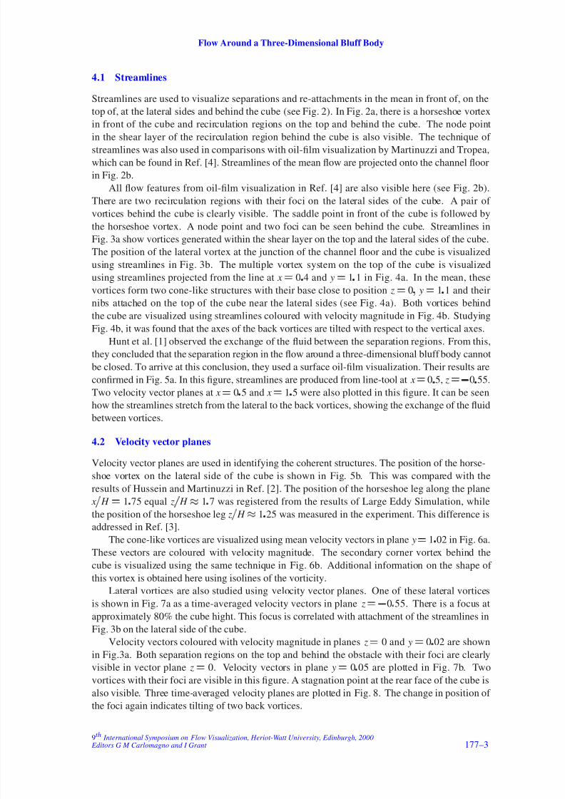
4.1 Streamlines

Streamlines are used to visualize separations and re-attachments in the mean in front of, on the

top of, at the lateral sides and behind the cube (see Fig. 2). In Fig. 2a, there is a horseshoe vortex

in front of the cube and recirculation regions on the top and behind the cube. The node point

in the shear layer of the recirculation region behind the cube is also visible. The technique of streamlines was also used in comparisons with oil-film visualization by Martinuzzi and Tropea,

which can be found in Ref. [4]. Streamlines of the mean flow are projected onto the channel floor

in Fig. 2b.

All flow features from oil-film visualization in Ref. [4] are also visible here (see Fig. 2b).

There are two recirculation regions with their foci on the lateral sides of the cube. A pair of

vortices behind the cube is clearly visible. The saddle point in front of the cube is followed by

the horseshoe vortex. A node point and two foci can be seen behind the cube. Streamlines in

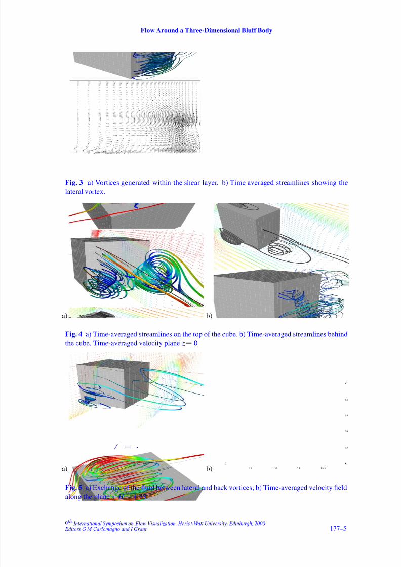
Fig. 3a show vortices generated within the shear layer on the top and the lateral sides of the cube.

The position of the lateral vortex at the junction of the channel floor and the cube is visualized

using streamlines in Fig. 3b. The multiple vortex system on the top of the cube is visualized

using streamlines projected from the line at x

0

4 and y

1

1 in Fig. 4a. In the mean, thesevortices form two cone-like structures with their base close to position z 0 y 1 1 and their

nibs attached on the top of the cube near the lateral sides (see Fig. 4a). Both vortices behind

the cube are visualized using streamlines coloured with velocity magnitude in Fig. 4b. Studying

Fig. 4b, it was found that the axes of the back vortices are tilted with respect to the vertical axes.

Hunt et al. [1] observed the exchange of the fluid between the separation regions. From this,

they concluded that the separation region in the flow around a three-dimensional bluff body cannot

be closed. To arrive at this conclusion, they used a surface oil-film visualization. Their results are

confirmed in Fig. 5a. In this figure, streamlines are produced from line-tool at x

0

5, z

0

55.

Two velocity vector planes at x

0

5 and x

1

5 were also plotted in this figure. It can be seen

how the streamlines stretch from the lateral to the back vortices, showing the exchange of the fluid

between vortices.

4.2 Velocity vector planes

Velocity vector planes are used in identifying the coherent structures. The position of the horse-

shoe vortex on the lateral side of the cube is shown in Fig. 5b. This was compared with the

results of Hussein and Martinuzzi in Ref. [2]. The position of the horseshoe leg along the plane

x

H

1

75 equal z

H

1

7 was registered from the results of Large Eddy Simulation, while

the position of the horseshoe leg z H 1 25 was measured in the experiment. This difference is

addressed in Ref. [3].

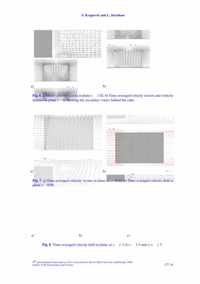
The cone-like vortices are visualized using mean velocity vectors in plane y

1

02 in Fig. 6a.

These vectors are coloured with velocity magnitude. The secondary corner vortex behind the

cube is visualized using the same technique in Fig. 6b. Additional information on the shape of

this vortex is obtained here using isolines of the vorticity.

Lateral vortices are also studied using velocity vector planes. One of these lateral vortices

is shown in Fig. 7a as a time-averaged velocity vectors in plane z

0

55. There is a focus at

approximately 80% the cube hight. This focus is correlated with attachment of the streamlines in

Fig. 3b on the lateral side of the cube.

Velocity vectors coloured with velocity magnitude in planes z

0 and y

0

02 are shown

in Fig.3a. Both separation regions on the top and behind the obstacle with their foci are clearly

visible in vector plane z

0. Velocity vectors in plane y

0

05 are plotted in Fig. 7b. Two

vortices with their foci are visible in this figure. A stagnation point at the rear face of the cube is

also visible. Three time-averaged velocity planes are plotted in Fig. 8. The change in position of

the foci again indicates tilting of two back vortices.

9th International Symposium on Flow Visualization, Heriot-Watt University, Edinburgh, 2000 Editors G M Carlomagno and I Grant 177–3



S. Krajnovic and L. Davidson

a)

b)

Fig. 2 Streamlines of the mean flow projected onto: a) the center-plane of the cube; b) the channel

floor.





a) b)

Fig. 6 a) Mean velocity vectors in plane y

1

02; b) Time-averaged velocity vectors and vorticity

isolines in plane z 0, showing the secondary vortex behind the cube.

a) b)

Fig. 7 a) Time-averaged velocity vectors in plane z 0 55; b) Time-averaged velocity field in

plane y

0

05.

a) b) c)

Fig. 8 Time-averaged velocity field in plane: a) x

1

3, b) x

1

5 and c) x

1

7.





a) b)

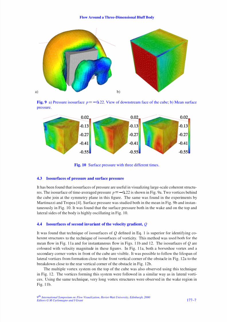
Fig. 9 a) Pressure isosurface p

0

22. View of downstream face of the cube; b) Mean surface

pressure.

Fig. 10 Surface pressure with three different times.

4.3 Isosurfaces of pressure and surface pressure

It has been found that isosurfaces of pressure are useful in visualizing large-scale coherent structu-

res. The isosurface of time-averaged pressure p

0

22 is shown in Fig. 9a. Two vortices behind

the cube join at the symmetry plane in this figure. The same was found in the experiments by

Martinuzzi and Tropea [4]. Surface pressure was studied both in the mean in Fig. 9b and instan-

taneously in Fig. 10. It was found that the surface pressure both in the wake and on the top and

lateral sides of the body is highly oscillating in Fig. 10.

4.4 Isosurfaces of second invariant of the velocity gradient, Q

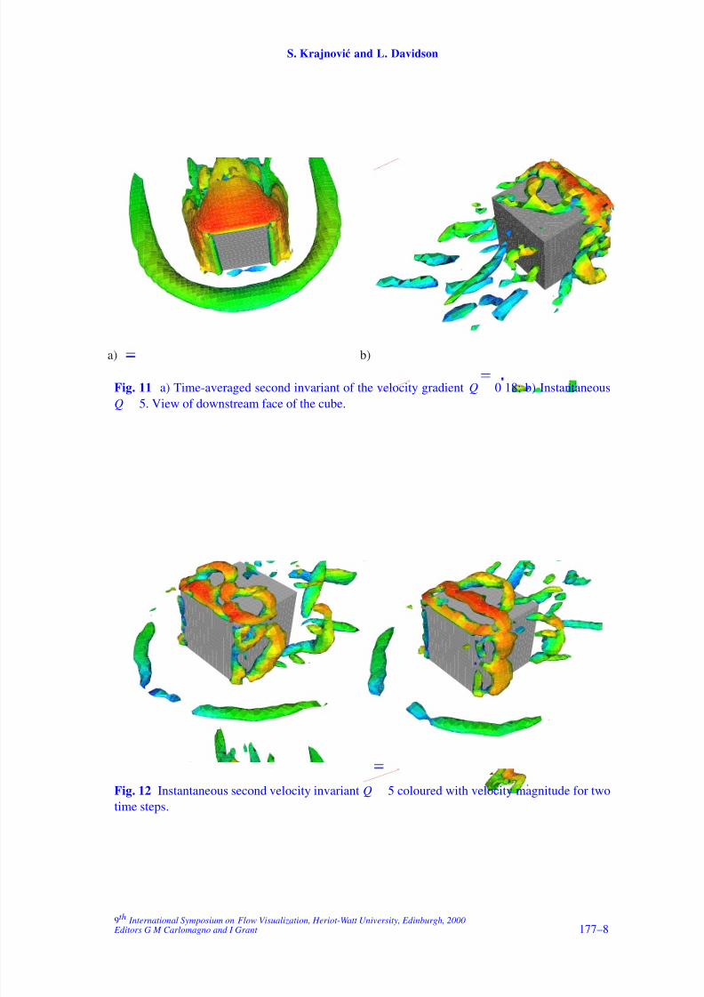
It was found that technique of isosurfaces of Q defined in Eq. 1 is superior for identifying co-

herent structures to the technique of isosurfaces of vorticity. This method was used both for the

mean flow in Fig. 11a and for instantaneous flow in Figs. 11b and 12. The isosurfaces of Q are

coloured with velocity magnitude in these figures. In Fig. 11a, both a horseshoe vortex and a

secondary corner vortex in front of the cube are visible. It was possible to follow the lifespan of

lateral vortices from formation close to the front vertical corner of the obstacle in Fig. 12a to the

breakdown close to the rear vertical corner of the obstacle in Fig. 12b.

The multiple vortex system on the top of the cube was also observed using this technique

in Fig. 12. The vortices forming this system were followed in a similar way as in lateral vorti-

ces. Using the same technique, very long vortex structures were observed in the wake region in

Fig. 11b.





a) b)

Fig. 11 a) Time-averaged second invariant of the velocity gradient Q

0

18; b) Instantaneous

Q

5. View of downstream face of the cube.

Fig. 12 Instantaneous second velocity invariant Q

5 coloured with velocity magnitude for two

time steps.





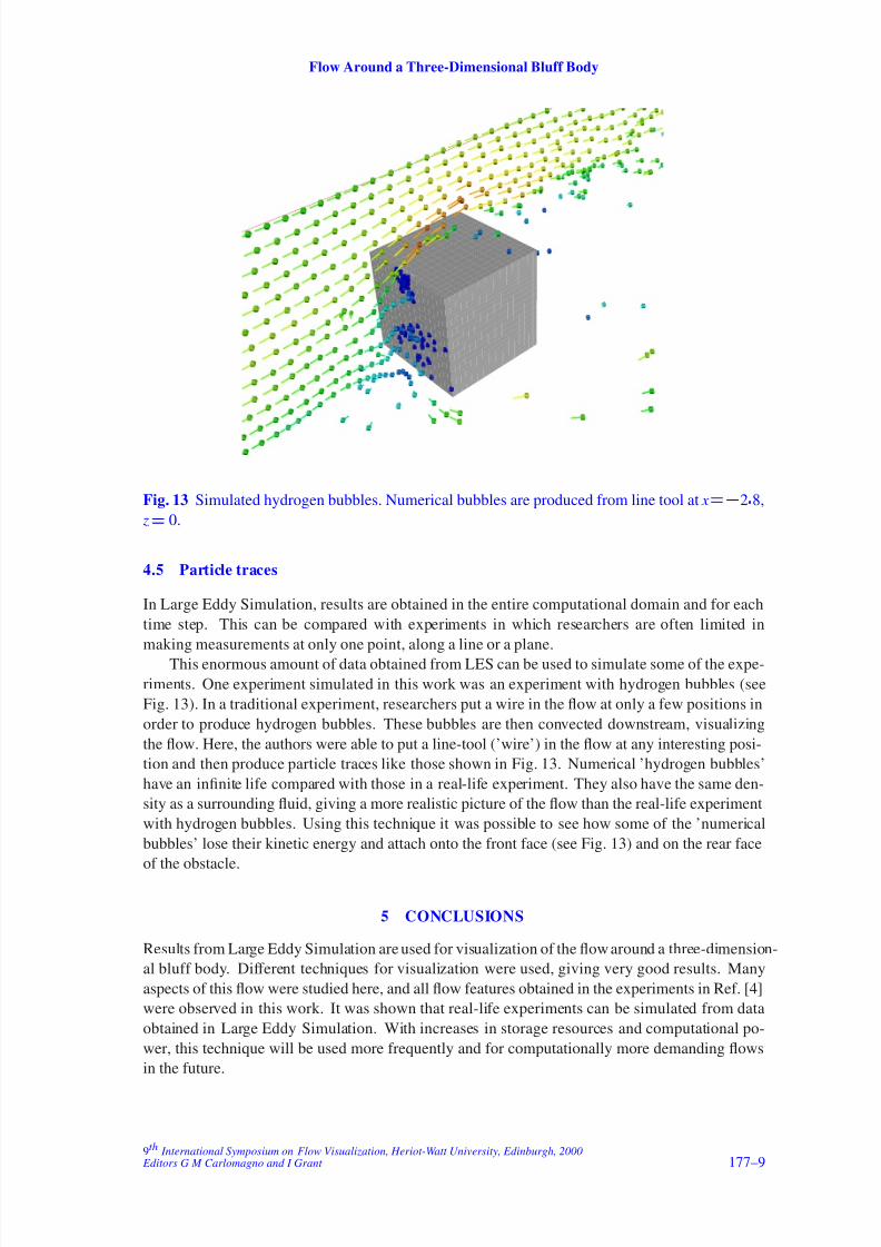
Fig. 13 Simulated hydrogen bubbles. Numerical bubbles are produced from line tool at x

2

8,

z

0.

4.5 Particle traces

In Large Eddy Simulation, results are obtained in the entire computational domain and for each

time step. This can be compared with experiments in which researchers are often limited in

making measurements at only one point, along a line or a plane.

This enormous amount of data obtained from LES can be used to simulate some of the expe-

riments. One experiment simulated in this work was an experiment with hydrogen bubbles (see

Fig. 13). In a traditional experiment, researchers put a wire in the flow at only a few positions in

order to produce hydrogen bubbles. These bubbles are then convected downstream, visualizing

the flow. Here, the authors were able to put a line-tool (’wire’) in the flow at any interesting posi-

tion and then produce particle traces like those shown in Fig. 13. Numerical ’hydrogen bubbles’

have an infinite life compared with those in a real-life experiment. They also have the same den-

sity as a surrounding fluid, giving a more realistic picture of the flow than the real-life experiment

with hydrogen bubbles. Using this technique it was possible to see how some of the ’numerical

bubbles’ lose their kinetic energy and attach onto the front face (see Fig. 13) and on the rear face

of the obstacle.

5 CONCLUSIONS

Results from Large Eddy Simulation are used for visualization of the flow around a three-dimension-

al bluff body. Different techniques for visualization were used, giving very good results. Many

aspects of this flow were studied here, and all flow features obtained in the experiments in Ref. [4]

were observed in this work. It was shown that real-life experiments can be simulated from data

obtained in Large Eddy Simulation. With increases in storage resources and computational po-

wer, this technique will be used more frequently and for computationally more demanding flows

in the future.





6 ACKNOWLEDGMENT

This work was supported by NUTEK and the Volvo Car Corporation.

REFERENCES

[1] J. C. R. Hunt, C. J. Abell, J. A. Peterka, and H. Woo. Kinematical studies of the flows around free

or surface-mounted obstacles; applying topology to flow visualization. Journal of Fluid Mechanics,

86:179–200, 1978.

[2] H.J. Hussein and R. J. Martinuzzi. Energy balance for turbulent flow around a surface mounted cube

placed in a channel. Physics of Fluids A, 8:764–780, 1996.

[3] S. Krajnovic. Large eddy simulation of the flow around a three-dimensional bluff body. Thesis

for Licentiate of Engineering 00/1, Dept. of Thermo and Fluid Dynamics, Chalmers University of

Technology, Gothenburg, Sweden, January 2000.

[4] R. Martinuzzi and C. Tropea. The flow around surface-mounted prismatic obstacles placed in a fully

developed channel flow. ASME: Journal of Fluids Engineering, 115:85–91, 1993.


sinisa edinburgh

Documents