sohrab abizadeh for the degree of doctor of philosophy
TRANSCRIPT

AN ABSTRACT OF THE THESIS OF
SOHRAB ABIZADEH for the degree of DOCTOR OF PHILOSOPHY
AGRICULTURAL AND in RESOURCE ECONOMICS presented on January 8, 1976
Title: TAX COMPONENTS AND THE DEGREE OF ECONOMIC
DEVELOPMENT
Abstract approved: ^ T V •*" '''^:'*li
JeVn B. Wckoff
Increased revenue is required for governments in less developed
countries to further their economic objectives. Besides foreign aid,
borrowing, and deficit financing, the theory of public finance suggests
that taxation is the prime source of revenue for development financing.
As governments perform their functions and raise revenue, problems
arise. Although many types of taxes are theoretically available,
there are only a few that can be practically employed at specific
stages of economic development.
Most of the taxation literature from less developed countries
has suggested different tax systems. The main objective of this stud^jN
was to explore opportunities that already exist for raising tax revenue
for expanding economic development. Direct as well as indirect taxes/
were analyzed in detail.
A quantitative appraisal of changes in tax components and their
relationships to the degree of economic development was conducted

The results of the quantitative analysis were explained within a
theoretical framework.
The hypotheses formed concentrated on ratios rather than
absolute values to eliminate the causality problem.
It was hypothesized that there is a direct relationship between
the degree of economic development and tax. components in a country's
total government revenue!. A number of linear regression models were I \ \ &<^
employed, using pooled cross-section, and time-series data, to l
examine the changes in tax components "explained" by reference to
changes in several independent variables representing the degree of
economic development. The use of time-series data did not make it
possible to reject the hypothesis that autoregression was present. The
Durbin approach was used to correct for autoregression in all the
models, which provided unbiased and more efficient statistical esti-
mates of the parameters involved.
An improved method of grouping countries by stage of economic^
development, using factor analysis, }was employed. This technique
grouped countries on the basis of a set of various indicators of socio-
economic well-being including per capita gross domestic product.
Three groups of countries were identified. Group one was labeled
"underdeveloped, " group two "developing, " and the third group,
"developed" countries.
+1

Tax revenue as a proportion of gross national product increased
with advancing development. Indirect taxes were a major component^
of the total taxes at all stages of development while direct taxes
became important for the group of developing countries.
Countries which shifted from one stage of development to
another increased their total tax revenue primarily through indirect j i
taxes. '
Empirical analysis was done examining the possibility of using
different taxes by an underdeveloped or developing country, with the
objective of increasing tax revenue. The empirical findings indicate
that: (a) indirect taxes offer the best source of revenue in under-
developed countries, and (b) although direct tax collection is possible,
developing countries encounter some problems in their collection when
just entering this stage. As the economy of these countries develops,
higher reliance on direct taxes can be implemented along with the
existing indirect taxes to maximize the governments' tax revenue.

Tax Components and the Degree of Economic Development
by
Sohrab Abizadeh
A THESIS
submitted to
Oregon State University
in partial fulfillment of the requirements for the
degree of
Doctor of Philosophy
Completed January 1976
Commencement June 1976

APPROVED:
Professo^ o^ Agricultural and Resource Economics in charge of major
f-/ = /f Head of Depantment of Agricultural and Resource Economics
Dean of Graduate School -a-
Date thesis is presented January 8, 1976
Typed by Mary Jo Stratton for Sohrab Abizadeh

AC KNOW LEDGMENTS
I am most appreciative of many individuals who have contributed
to my graduate training and the preparation of this thesis. In
particular, debts of gratitude are due to:
Dr. Jean B. Wyckoff, major professor, for his professional
guidance and valuable time during the course of this research and
years of graduate study.
Drs. James B. Fitch, Joe B. Stevens, and R. Charles Vars,
Jr. for providing many valuable comments and very willingly offering
advice during the progress of this dissertation.
Dean Carl H. Stoltenberg, Graduate School Representative,
for valuable time.
Finally, to my wife, Faegheh, for encouragement, and our
little son, Arash, for patience.

TABLE OF CONTENTS
Page
I. INTRODUCTION AND PROBLEM IDENTIFICATION 1
Introduction ^L, Problem Statement ^Zy The Objectives g§?)
II. DEVELOPMENT OF THE HYPOTHESES AND PAST STUDIES 12
Statement of the Hypotheses: A Theoretical Framework 12
Past Studies 25
III. SOURCES AND NATURE OF THE DATA AND THE VARIABLES 32
The Data 33 Gross Domestic Product (GDP) 33 Information on Taxes and Tax Revenue 36 Information on Expenditure 37 Financial Statistics 39 Trade Statistics 39 Population 40
The Variables 40
IV. GROUPING OF THE SAMPLE COUNTRIES 48
■V. METHODOLOGY AND TESTING THE HYPOTHESES (5?)
Total Tax Ratio 59 Interpreting the Results 66 Conclusions and Generalization 78
Direct Tax Ratio 80 Interpreting the Results 86 Conclusions and Generalization 94
Tax Structural Stability 96 Interpreting the Results 98 Conclusions and Generalization • 98
Indirect and International Trade Taxes 100 Conclusion and Generalization 104

Page
International Trade Taxes 104 Interpreting the Results 106 Conclusions and Generalization 111
The Case of Highly Developed Countries 112 Interpreting the Results 115 Conclusions and Generalization 118
The Group of Countries which Shifted through Time 119 Interpreting the Results 125 Conclusions and Generalization 130
VI. CONCLUDING REMARKS
Summary 132 Conclusions 134 Implications and Speculations 137 Suggestions for Further Research 142
BIBLIOGRAPHY 144

LIST OF TABLES
Table Page
1 List of the countries for which data were collected. 34
2 Table of dependent and independent variables. 41
3 Cumulative percentages of three factors for the first decade. 50
4 . Cumulative percentages of four factors for the first decade. 50
5 Cumulative percentages of three factors for the second decade. 50
6 Cumulative percentages of four factors for the second decade. 50
7 Classification of the countries based on highest factor loading--first decade. 52
8 Classification of the countries based on highest factor loading-- second decade. 52
9 Grouping of the countries by factor analysis, the first decade. 53
10 Grouping of the countries by factor analysis, the second decade. 54
11 Comparison of factor analysis and per capita GDP for the first decade. 56
12 Comparison of factor analysis and per capita GDP for the second decade. 57
13 List of the countries which shifted their group. 58
14 Summary table of regression analyses for total tax ratio (TR). 61
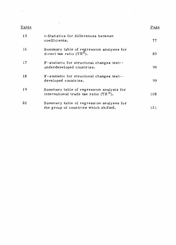
Table Page
15 t-Statistics for differences between coefficients. 77
16 Summary table of regression analyses for direct tax ratio (TR ). 83
17 F-statistic for structural changes test-- underdeyeloped countries. 99
18 F-statistic for structural changes test-- developed countries. 99
19 Summary table of regression analysis for international trade tax ratio (TR ). 108
20 Summary table of regression analyses for the group of countries which shifted. 121

TAX COMPONENTS AND THE DEGREE OF ECONOMIC DEVELOPMENT
I. INTRODUCTION AND PROBLEM IDENTIFICATION
Introduction
Research in the area of public finance has traditionally concen-
trated on the economic impact of taxes and government expenditure
upon a region or a country.
However, in recent years much of the applied and theoretical
work has been related to the task of constructing tax systems suited
to the particular economic and social conditions prevailing in various
countries. The following is an international study of the governmental
tax revenue and its components, in different countries at different
stages of economic development. The major objective was to find,
through a systematic statistical analysis, the relationship between
taxation and the degree of economic development, and more impor-
tantly, how the composition of total taxes changed in the course of
economic development.
The methodology consisted of a number of short-run as well as
long-run analyses. Cross- section, time-series, and pooledcross-
section-time-series data were analyzed.
The analysis started with the examination of total tax revenue as
a percentage of gross donaestic product (GE)P) and its j^lationshig,
with the degree of economic development. Next total tax revenue and
its comjaonentg,, mainly direct and indirect taxes, were analyzed.
Finally, attention was focused on those countries which passed through
their so called (transition period,, to fall under a group of more
developed countries. Examination of the tax structure of these
countries along with the statistical results obtained from the former
analyses provided a framework for speculating on possible tax policies
for the group of less developed countries (LDCs).
Problem Statement
Social awareness and mass communication have resulted in a
public demand for economic advancement and achievement of higher
standards of living in the less developed countries (LDCs). Political
leaders of these countries, recognize the importance of this demand,
and it is virtually impossible in today's world to find a country whose
government has not attempted to improve its economy. In fact,
econonaic development and growth have become important goals in both
developed and less developed countries.
It might be argued that objectives other than econonaic develop-
ment should be taken into account when examining policy alternatives.
It is believed that by focusing on economic development and growth,

most of the other desired objectives, being primarily social or econo-
mic and relating to the distribution of income, will be accomplished
(Ture, 1973, especially pp. 3-7).
LDCs need increased savings and investment to achieve their
economic development objec,ty/e. Savings can take place in either the
private or public sectors. The main sources of saving bv the public
sector are foreign aid, retained earnings of public corporations,
deficit financing, printing money, and taxation. The private sector
can save and invest out of disposable income. High levels of savings
and investment in the private sector are dependent on factors which
are frequently lacking in the LDCs.
There is little hope that the private sector has either the poten- x
l. tial or the ability to greatly increase its savings and investment.
There are at least two reasons for the existence of this situation. The
first is that the majority of the people are poor in the sense that their
income is below the subsistence level. "In developing countries, the
majority of households may hoard some banknotes or seeds to be used
in case of emergency, but they are too poor to save in other forms"
(Van Mensbrugghe, 1972, pp. 36-37). Those able to save are the
wealthy families. And, if we accept Snyder's (1974) conclusion that
wealth tends to affect savings available for investment negatively in
the LDCs, then significant private saving may not occur in the private
sector.

Even if those who are able to save engage in saving activities,
there is still no guarantee that their savings will neces^sarily be ^
received_in. a form that can_be channeled into,.pr.ad.u.ciivje-.in.v.e.s.tme.Rt.,
Instead of holding deposits with banks, shares, and other financial
investments, ". . . saving has taken the form of buying gold, silver,
acquiring stocks of commodities for speculation, and so forth"
(Basch, 1964, p. 106).
A second reason for insufficiency of private investment of the
LDCs is the result of inadequately developed banking systems. Com-
mercial banks in the LDCs cannot create demand credits to finance
worthwhile projects in private sector because:
In the least developed countries, goods and services are purchased with legal tender notes and coinage and not with cheques or bank demand deposit. One per cent or less of the families" own such deposits anyway (Enke, 1967/pp, 257-58).
Furthermore, financial institutions and banking systems in these
countries are not prepared to transfer individuals' savings into pro-
ductive investment (Cf. Due 1963, p. 18).
The statement that private sectors in LDCs do not save and if they do their savings are not channeled into productive investment, does not mean that the private sector should be totally neglected in the process, or e^ven starting, of economic advancement. On the con- trary, along with the increase in government revenue and, thus saving, it is expected that planners in LDCs will take the private sector initiative into serious account and establish policies to motivate as well as facilitate saving, and thus productive investment, in that sector. Those interested are referred to Basch (1964) especially Chapters 5, 7, and 8. Also see Van Mensbrugghe (1972) and Snyder (1974).

An alternative source of investment is to attract foreign capital
into the country. This source often fails either because of high risk,
2 a low level of infrastructure, low total demand, possibility of revolu-
tion and nationalization of foreign capital.
Bangs argues that, in order for investment to be undertaken by
the private sector, an economic climate in which private investment
can fluorish is vital. He lists some of the elements necessary to
create such an economic clinnate, all of which are directly related to
the level of economic development of the country (1968, pp. 99-100).
Other barriers to development exist in the private sector.
Public utilities are not proyidecj, privately because the amount of
investment involved is too large. There is also a degree of uncer- i
tainty and risk involved in investment, especially in the early stages ,
1 of economic development, since there is a possibility that the public /
will not welcome a specific project. Furthermore, the prospect of
future returns from these investments is usually too remote and too
low to attract private investors. Davidson contends that the govern-
ment is the only organization able to perform such functions.
There has been a rapid expansion in the belief that many things cannot be left to the workings of the underdeveloped market system but rather that it is the duty of the govern- ment to provide the desired goods and services, either by
2 Because most of the less developed countries are small in population.

purchase or by production and to carry through substantial programs of redistribution of real income between different sectors of the society (Davidson 1967, p. 229).
The existing barriers^to the_ creati.Qn ,of highe,i!„sa5f,ingts,.and
investment in the private sector may necessitate direct government
intervention in promoting inve.strnent. While the emphasis on the
public sector may vary between LDCs, in nearly all LDCs a steady
increase in governmental functions is required. Due, in studying the
economies of eight African countries, argues that, in all of these
countries, in varying degrees, there is an acceptance of the principle
that some government participation is required. The slow rate of
growth in the past is taken as irrefutable evidence that the govern-
ment must act to speed up the process, to increase the rate of
industrialization, and to direct the types of production most signifi-
cant in terms of economic development (1963, p. 18). Chelliah
states that it is the responsibility of the government to perform the
saving function;
. . . the primary task of fiscal policy in underdeveloped countries is to raise the ratio of savings to national income. . . . This means that the role of fiscal policy in underdeveloped countries essentially has to be allocative (1969, p. 44. Also see p. 52).
Indeed, the largest number of suggestions regarding the objective of
fiscal systems have basically one common objective--that of nnobiliz-
ing resources from the private sector to the government sector (Cf.
Chelliah 1969, p. 52; Due 1963, p. 146; Hicks 1965, pp. 67-68).

Under these circumstances, where the private sector is not.
active in creating enough saving and investment for launching econo-
mic development, government.saying.j)]jiys the crucial role. Genera-
tion of government savings for investment is very important, and has
assumed a growing importance in LDCs, particularly in countries
where the government is unable to borrow from the market because
of inadequate financial organization and lack of transf err able
3 savings. Finally;
In developing countries, government savings are especially needed to finance the building of transport facilities and the establishment of public utilities that are a prerequisite to economic development. In a number of countries they are also needed to compensate for the lack of or inadequacy of private investment in the business sector (Van Mensbrugghe, 1972, p. 38).
3 Martin and Lewis contend that the idea of government being exposed as the major source of saving is justified by three objec- tives:
First, the amount of private savings in under-developed coun- tries is relatively small, and so also is the amount available through international investment. Hence if a large investment programme is to be financed it must be through forced savings, and this is more equitably achieved through taxation than through inflation. Secondly, some developed countries have exactly the same problem, of tendency for investment to exceed savings, and the prescription of a budget surplus to counter inflation in these circumstances is exactly the same solution reached by a different road. Thirdly, socialistic governments are anxious that new capital be created on public rather than private account, and since all capital is created out of saving the only way to prevent private fortunes from growing pari passu with capital formation is to finance capital out of public rather than private saving (1956, p. 212,).

8
( Two of the meansNby which government can i(ggre<age_j3avi.ng8„
are; (1) budget surpluses (excess of revenue over expenditure), and
(2) the transfer of retained earnings and other revenue of government
corporations. The second procedure seems to fail in the case of
LDCs, because many government owned enterprises tend to incur
losses in the early stages of development. The underlying reason is
that the government usually tends to undertake activities which private
enterprise does not find profitable at that particular time. Therefore,
the only real source by which government can increase its saving is
through an excess of revenue over expenditurg^,.^ This can be done via
taxation. "Developing countries must to a very large extent finance
internally their development programs. The primary means of
internal financing available to such countries is taxation" (Cutt, 1969,
p. 38 3). Given the comparatively limited amounts of resources that it
is ordinarily possible and prudent to obtain from abroad and from
domestic borrowing and nontax revenues, most of the LDCs have felt
the need to increase tax revenues (Cf. Chelliah 1971, p. 254).
The main question is, how much can the government rely on
taxation as a source of revenue with the kinds of difficulties it faces
regarding effective tax collection? This question leads us to a kind
of "vicious circle. " Needs for public goods and economic growth
are developed; the private sector is not able to meet these require-
ments; the government is the only agent that can perform such

functions; a high amount of expenditure and, consequently, revenue is
required; one of the most important sources of revenue is taxation;
the backward social, economic, political and administrative struc-
tures do not make it feasible to collect tax easily; thus, government is
not able to finance those public goods and other investments which are
demanded by the public. /'
The question, then, is how and in what ways have the govern-
ments in less developed countries increased their tax revenue, during
the last two decades, given all the barriers that existed? What is the
relationship between taxation and the degree of economic development
in less developed countries as well as developed countries ?
An attempt was made to provide an answer to these fundamen-
tal questions.
Taxation opportunities that already exist in these countries,
given their economic condition, were explored through empirical
analyses. It was believed that while the capacity in LDCs is lower
than that of advanced countries, it was not accepted that the existing
tax revenue reflects the real tax potential. The problem was to work
out a system that would pin-point existing but unexplored tax sources
and take advantage of them.
There is obviously an inherent difficulty in establishing the
taxable capacity of various countries. No specific type of taxation
seems to exist that could be applied indiscriminantly to all LDCs.

10
But, pointing out real tax potentials is a useful step. The mere fact
that no general tax policy can be recommended for all JLDCs should
not prevent one from exploring possible tax sources, from which the
revenue can be used to hasten economic development.
The Obiectives
This study is both theoretical and empirical. It uses inter-
national data to test different hypothesized economic models and
submodels to reveal the relationship between the tax components in
total government revenue and economic development^ The empirical
findings, interpreted with the aid of theoretical concepts, prqvide^the
basis for policy speculations. There is no doubt that tax revenue has
been growing faster than GNP in LDCs with a consequent rise in tax
4 , ratio (Chelliah 1971, pp. 260-67). However, the objective here ^^\f\
to find out what happened to the components of tax revenue„.as__e£^n^-!
mies^develqp^d, regardless of the absolute or relative jnc,r_ease.^nd/i
or decrease in total tax j-eyenue. This.was. done to, explore the rela-I
i tive importance of different types of .taxes- a.L.diffexent^Leji&fel&^of
development. Any higher revenues obtained through these sources
could be used for promoting economic development.
4 . Tax rati6Mirdv'ii'sda"liy'"deflined as the ratio 6'f all'taxes and tax-like charges (including gross social security contribution from private sector, if any) t6 g'ross national product (GNP).

11
Two specific objectives were identified:
1. To provide a quantitative appraisal of chang^es^jn J:ax^
c5IS.B°^SI^1:J^?L§.->t^L§J6coSPJP5■y_^-?■V.?lS=fi§.•
2. To interpret the results of the quantitatiYe_-anal-vais with the
appropriate theoretical framework, as a possible basis..fpra
policy formulation to increase tax revenue.

12
II. DEVELOPMENT OF THE HYPOTHESES AND PAST STUDIES
Statement of the Hypotheses; A Theoretical Framework
This study contrasts the revenue structure of countries at
different levels of economic development. The main purpose is to
determine how the pattern of government tax revenue changes and to
identify the tax revenue patterns that are most appropriately asso-
ciated with different degrees of economic development.
The main objective, in the dirst stage, is not to explain
causality-whether it is higher economic development that results in
5 higher tax revenue or vice versa --rather it is to see how total
government tax revenue changes as the economy develops. Certain
observers have noted that the more developed economies character-
istically have higher ratios of taxation to national product than do the
LDCs (Hinrichs 1966, Musgrave 1969). Also there are those who
believe that the tax system that results in a higher percentage of tax
revenue in relation to national income or GNP is the better one. This
is possible if the country is developed or at least in the process of
developing (Krause, 196l, p. 213; Wheatcraft in Cadman, 1969, p.-73).
5 It is the total government tax revenue as a source of public invest- ment fund—which is important.
13
Bangs, however, claims that "While these associations may hold
generally between the advanced and less advanced countries, they are
not very accurate as indicators within the group of developing coun-
tries, considered by themselves" (1968, p. 14). This conclusion,
was not derived from a thorough empirical study. As a consequence,
the first hypothesis tested in this study was, 1) that there is a direct
relationship between the degree of economic development and the tax
ratio. A subhypothesis is, (1-a) that the above relationship holds
between developed and less developed countries as a whole as well as
within a group of underdeveloped, a group of developing and/or
developed countries.
To test this hypothesis, the data was divided into two decades--
the first decade, 1950-1959, and the second decade, 1960-1972.
Further, the sample of countries was separated into three groups
7 using factor analysis. This technique grouped countries on the basis
of a set of various indicators of socio-economic well-being including
per capita income, which traditionally has been used to group coun-
tries in past studies. Group one is labeled "underdeveloped
countries, " group two "developing countries," and the third group,
g "developed countries, " in our subsequent analysis.
The same type of division is used throughout the study. 7 See the chapter on Grouping of the Sample Countries, pp. 48-58.
0 This type of grouping is used throughout the study in order to deter- mine whether the relationships that hold for all the countries still

14
There is one type of change in taxation which is theoretically
attributed to the degree of economic development, i. e. , the change in
tax components or the relative importance of specified individual
9 taxes in the tax system, which is apt to change only as the economy
develops. Statements such as "Generally, however, tax systems
have tended to be more of a determined than determining factor"
(Hinrichs 1966, p. 63) are frequently made. Bangs (1968) makes
even a stronger assertion when he says, "The tax changes are, in
main, effects rather than causes of economic progress" (p. 15). He
also believes that direct taxes are applicable only to those economies
which have passed a certain stage of development (pp. 15-16).
hold when the countries are grouped on the basis of their degree of economic development. Also classifications of this sort enabled us to reject or verify the conclusions arrived at by other observers. Hinrichs (1966) finds that "openness, " not per capita income, is a key determinant of government revenue shares of GNP for under- developed countries (those countries with per capita income below $300). He also concludes that for countries with per capita incomes between $300 and $750, a strong, positive relationship exists between government revenue shares and per capita income (p. 19). The classification scheme used by Hinrichs is apparently arbitrary. Using our classification, an attempt was made to find out if Hinrichs1
conclusions still held. Hinrichs also concluded that a high level of development (per capita income above $750) is a sufficient, though not necessary, condition for a government revenue share of 18 per- cent or greater (p. 19). This is another way of saying that per capita income is a good explanatory variable for the variations in government revenue shares. This was also investigated.
9 The group of taxes to which individuals and businesses in a given country are subject is called the "tax system" or the "tax structure. "

15
If changes in the tax components, made feasible because of a
higher degree of economic development, also result in higher tax
revenue for the government, and if it is maintained that higher taxes
result in economic development, then exploration of new sources of
tax revenue is worth trying. The question then is, what happens to
the components of total government tax revenue as the economy
develops ?
Many authors have noted that the extent of reliance on direct
taxation usually increases with greater economic development
(Hinrichs 1966).
When comparing the feasibility of direct tax collection in less
developed countries with that of more developed countries, the
following points can be made.
(1) Corporate taxes are usually levied at a flat rate on all
companies in most less developed countries. Clearly, not too much
revenue has been generated by such a levy, because (a) company
income is often only a small part of national income in many
underdeveloped countries; (b) if the tax on companies were high,
there might be less incentive for private investment; (c) new com-
panies do not have any revenue to be taixed, and (d) more importantly,
. . . there takes place a substantial avoidance of the tax on corporate profits in underdeveloped countries because of the

16
'loophole' in the law in the form of the system of prerequi- sites such as office-provided cars, living accommodation, travel expense accounts in general which are charged off to business expenses (Tripathy 1968, p. 201).
(2) It can be argued that taxes on capital values, whether of
land or property, are likely to have a less adverse effect on incen-
tives to work and save than many forms of direct and indirect
taxation.
The problem in underdeveloped countries has been that usually
the owners of capital assets have had a high degree of control over
political institutions, through which they could influence tax legisla-
tion in their favor. Goode points out that: "Intensive use of the
property tax is blocked in most Latin American countries by a small
but politically powerful group of large land owners" (1964, p. 178).
This is true in most underdeveloped countries--especially if an old
system of land ownership exists (i.e., if a so-called land reform has
not taken place). Lack of records, difficulties in appraising the
properties and comparatively low tax yield through this type of tax
are some of the reasons behind their lack of emphasis. "In many
countries taxation of agricultural, particularly land tax, does not
yield amounts considered adequate when compared with taxation of
other sectors" (Basch 1964 , p. 95).
Thus, unless there are some changes in the social, economic,
and political institution of these countries, adoption of capital and

17
wealth taxes--without wholesale evasion--would seem to be
impracticable in less developed countries.
(3) In underdeveloped countries, personal incorine tax
generally has had a very limited coverage. It frequently has not been
applied to the agricultural sector, for constitutional or administrative
reasons. Hence, personal income tax has played a less significant
role in the tax structure of underdeveloped countries than in the more
developed countries.
It would seem that there are four reasons for the radically
different performance of personal income tax in underdeveloped
countries. First, there are problems in defining income. Second,
there are difficulties in assessing any one individual's income, even if
one knows how to define income. In underdeveloped countries, a
large sector of the economy is non-monetary, and wage-earners,
independent craftsmen, and small shop-keepers cannot read and write
well enough to fill out the simplest income tax return. Sometimes,
even if income earners are so literate as to be able to keep records
of their income, one can hardly rely on such documents; as in
developed countries, more than one set of income records can be
kept in order to avoid tax payment. Actually, in most low income
countries, some businessmen keep no books at all, while others
maintain two or more sets (see Goode 1964). With underdeveloped
banking and credit systems, it is difficult to trace business transactions

18
when they are all conducted in cash or barter. The third reason for
the radically different performance of personal income tax is related
to the fixing of tax rates and allowances. It is usually difficult to fully
apply the rates of taxation of developed countries to many of the less
developed countries. The degree of difference between the income
distribution pyramids in the countries is the key. If one applies the
tax rates found in the U.S. to, say, Egypt or Iraq, it makes a lot of
difference whether they are applied at the same absolute level of
income or at the same relative level of income. Suppose that a man
earning $1500 a year in the U.S. pays 5 percent of his income in tax
whereas a man earning $3000 pays 25 percent. Then one will not
obtain the same ratio of tax revenue to income in a poor country as
in the U.S. (if one applies these rates as they stand), for the simple
reason that the proportion of total income in these ranges is far less
in a poorer country ( cf, Prest 1962, pp. 32-35).
The fourth difficulty is with regard to the collection of taxes.
Voluntary tax; payment is not common in underdeveloped countries.
The alternative to this is application of the pay-as-you-earn system.
The latter approach covers only a small group of income earners in
the community and therefore raises the question of equality (i.e.,
only part of the income earners are subject to tax).
Voluntary income tax payment is an "ideal" in an underdeveloped
country. An efficient income tax can be used when an effective system

19
of political democracy exists. It is under such circumstances that
higher income people, constituting the only group that can pay income
taxes, would be obliged to accept the principle of a prevailing income
tax policy. However, in most of such countries an effective system
of political democracy is not likely to exist.
It is no accident that the more developed countries have used such indirect taxes as custom duties, property taxes, and excise taxes at the very early stages in their own develop- ment, and have gradually progressed from these levies to the more sophisticated and different forms of direct taxes, such as personal and corporation income levies (Bangs 1968 pp. 135-36).
These ideas were formulated as a general hypothesis and tested by a
model involving variables which represent and reflect the degree of
economic development as independent variables and direct tax ratio
(total direct tax revenue divided by total tax revenue) as the dependent
variable. The hypothesis is, 2) that as the economy develops the tax
structure of the country changes towards more intensive use of direct
taxes, i.e., the relative proportion of direct and indirect tax changes
towards a higher and higher direct tax ratio. Accordingly, other
10 By "political democracy" it is meant the elimination of any possible domination of a few "landed" individuals regarding such things as laws, including tax legislation.
It was believed that, although this hypothesis generally may hold, exceptions may exist. Those exceptions were tested for by generating a new group of countries, using an additional criterion, that of a regional factor. The new group was called "highly developed" and consisted of countries of Western Europe and North America.

20
models with corresponding data were used to test similar hypotheses
for different periods of time for the same groups of countries,
different groups in the same period of time, and the same group using
all the years. This was done to see if the results obtained supported
or rejected the idea stated by Bangs that such an association may not
hold within the group of underdeveloped or developing countries,
considered by themselves (see Bangs 1968, p. 14).
It was also hypothesized, 3) that the underdeveloped countries
possess a more unstable tax structure than those of more developed
countries, i.e., the group of underdeveloped countries exercises a
more irregular change in their tax components than that of developed
countries. This was evaluated by both short-run and long-run
analyses. Using the first group in the first decade and running a
regression for years 1950, 1955, and 1959. gave a clear picture of the
structural changes for this group of countries. The independent
variable used was direct tax ratio (defined as direct taxes divided by
total tax revenue).
The same type of analysis was performed for the first group in
the second decade using data for years I960, 1965, and 1970, and
was repeated for the third group. Comparison of the results obtained
through these analyses, together with the Chow test, provided a
framework for our conclusions.
21
Having dealt with the direct tax ratio and its relationship with
the degree of economic development, the study proceeded to deal with
indirect taxes (including international trade taxes) and their relation
to economic development.
According to Hinrichs (1966) indirect taxes still predominate
12 in the middle stage of economic development. The breakdown of
countries into three groups has enabled us to shed more light on this
situation.
As a result of the social and cultural background that exists in
underdeveloped countries, most of the public thinks of taxes as
forced and unnecessary payment to government. Thus it would seem
logical for governments of those countries to collect as much tax as
possible via channels that are not considered direct payments to the
government. Still, such taxes may be virtually nonexistent in some
of these underdeveloped countries.
An attempt was made to identify that group or those groups of
countries which may fall into this category. To accomplish this, the
following hypothesis was formulated, 4) that for the first group in the
first decade, the bulk of the tax revenue was collected through indirect
taxes including taxes on international trade, i. e. , the group of under-
developed countries in the first decade collected taxes whose direct
12 His middle stage refers to those countries with per capita income between $250-$500.

22
impact on the public was minimized, or at least disguised. Inter-
national trade taxes meet this criterion. The same hypothesis applies
to the group of underdeveloped countries in the second decade.
The approach used to test this hypothesis was that of comparing
the mean of the indirect and trade tax ratio (defined as all indirect
taxes including trade taxes divided by total tax. revenue) of under-
developed countries for each decade and testing the null hypothesis
to see if this mean is greater than the grand mean of all countries,
excluding the group of underdeveloped countries.
It is often argued that the major source of taxation in the LDCs
is taxes on international trade (see Davidson 1965, p. 4). As one of
the components of international trade taxes, import duties have played
an important role in the revenue structure of LDCs. Import duties
have been used in two different ways: first, as a protective device
aimed at prohibiting the imports of commodities into the country and,
second, as a source of revenue for government. The reason for the
importance of import duties has been partly historical; i.e., imports
were the basis from which the cash economy permeated the country,
were concentrated and visible. Also, if the imports constituted a
large part of GDP, it was considered reasonable to tax them.
Exports from a less developed country often consist of only one
or at most two, main products. Since the proportion of export taxes
to total government tax revenue often is already high, further increases
23
in export taxes are likely to place the country at a competitive dis-
advantage compared with its rival suppliers. This limits the feasibility
of further reliance on exports taxes unless all competing countries
follow similar policies.
If the exports of a country account for a large fraction of the
world supply and have an inelastic demand, then when export taxes
are increased, the resulting contraction of output will raise the world
price relatively more and part of the export tax will be passed on to
foreign consumers. This may be but a temporary phenomenon which
may be brought to an end with the development of substitutes and
alternate sources of supply, encouraged by the high export taxes.
On the other hand, for a country that is a small producer and
exporter of a commodity, the demand for its exports will be relatively
elastic. Any increase in price resulting from higher export taxes may
drive its customers to other suppliers who are selling at the world
price. In this case higher export tax is borne by the domestic pro-
ducers of the exporting country. The use of the higher export tax
increases the cost of production to the domestic producer if he is to
maintain his volume of export sales and, thus, reduce his net rate of
return. If the reduction in the net return makes the business unprofit-
able and results in the closing down of operation, economic develop-
ment may be impeded.

24
However, because of the ease of administration, a higher
reliance on trade taxes is sometimes recommended. On the other
hand, the number and importance of the trade agreements have
increased in recent years. To see if the relative importance of such
taxes had increased during the first decade and decreased during the
recent years, for the group of underdeveloped and developing coun-
tries (LDCs), it was hypothesized that, 5) the relative reliance on
international trade taxes had increased and peaked in the first decade,
then decreased during the second decade.
Two separate regression models were used--one using the
data from the first decade combining underdeveloped and developing
countries, and the other using second decade data for the same group.
Trade tax ratio (defined as international trade taxes divided by total
tax revenue) was used as the dependent variable.
The hypothesis was tested in a more general form by using all
the countries in each decade and comparing the results. It became
possible to determine whether international trade agreements, which
have gained in relative strength in recent years, have been effective.
Effectiveness was expressed in terms of less relative reliance on
international trade taxes.
We further hypothesized, 6) that countries, such as those in
Western Europe and North America, due to their high degree of
economic development have been able to increase their relative

25
reliance on sophisticated techniques of tax collection and thus,
increased their indirect tax ratio (defined as indirect taxes, excluding
trade taxes, divided by total tax revenue) in the second decade as
their economy developed. A regression model with indirect tax ratio
as the dependent variable and factors representing the degree of
economic development as independent variables was employed to test
this hypothesis.
Besides the results obtained from the above analyses, it was
felt that policy implications might be derived from the experiences
of those countries which shifted from one group in the first decade
to another group in the second decade. The evaluation of their tax
structures during this transition and the fiscal reasons behind the
changes were examined. Since more than one country had shifted to
another group, pooled, cross-section, time-series analysis was used
to determine those hypotheses that were to be maintained or rejected
as a base for policy.
Past Studies
Tax structural differences and potential tax performance of any
country can be attributed to different economic structures as well as
other factors and circumstances. Various attempts haye been made
during the last two decades to provide "scientific" explanations of tax
ratio differences and changes in tax components with the hope that a
26
policy formula could emerge. These studies have similarities as
well as dissimilarities.. The objective, at this point, is not to conduct
a comparative analysis of the past studies but to explain the similari-
ties and dissimilarities among past studies in light of the results of
this study.
Martin and Lewis (1956) compared the revenues and expenditures
of 16 countries at different levels of economic development. Their
main objective was to see how patterns of expenditure and sources of
revenue varied with economic development and what patterns of taxes
and expenditure are appropriate to different levels of development.
Williamson (196l) in a follow-up of Martin and Lewis' study
took more countries and a longer time period (1951-56), including 17
developed countries with tax ratios ranging between 20 and 35 percent
and 15 LDCs ranging between 9 and 21 percent. He found a close fit
with a correlation coefficient of 0.73. Both of the above mentioned
studies concentrated on public expenditure and revenue and their
relationship to per capita national income. Their analyses involved
univariate regression with per capita national income as the indepen-
dent variable. Williamson uses pooled cross-section and time-series
data for a period of time so short that it hardly provides enough time
for a country to change its degree of economic development. This
type of analysis, along with the careful selection of sample countries,

27
reflecting a wide range of economic development and almost continu-
ous tax; ratios, should result in a "good fit. "
Hinrichs (1965) questioned the former findings and tried to
present a "better" explanation for the tax changes through a multiple
regression study of 60 countries using data from the years 1957-60
(a shorter period than that of Williamson). He makes the implicit
assumption that per capita income is the only criteria to be us^d as an
indicator of the degree of economic development. Consequently, if
there are other variables which explain tax ratio changes better than
per capita national income, the conclusion that the tax ratio is
related to the degree of economic development, as reflected by per
capita income, should be rejected. He states;
Conventional wisdom holds that government revenue shares of gross national product increase with economic development. This is obvious when contrasting the level of government revenue shares between developed and less-developed countries. However, when observing differences among less-developed countries only, this proposition is misleading at best or at worst just plain wrong (p. 564).
However, his conclusion is that openness may serve as a much better
estimation for poor countries of 'taxable capacity1 than the usual per
capita income measure. As he points out
The greater the size of the foreign-trade sector, quite probably the greater is the degree of monetization of the economy, the predominance of 'cash ' crops rather than subsistence agriculture, the size of business units, the extent of urbanization and industrialization (pp. 554-55).

28
Openness is, by itself, an indicator of the degree of economic develop-
ment. Thus, if openness is related to tax ratio changes for LDCs, it
follows that the same proposition could be applied to developed
countries with regard to the tax ratio and the degree of economic
development. Per capita income is not the only factor that can be
used as an indicator of the degree of economic development.
Hinrichs (1966) in his more thorough study of taxes attempted to
deal with both tax ratio and tax components changes during the course
of economic development. He performs a multiple regression study
of 60 countries for the period 1957-60 in order to identify the deter-
minants of government revenue as a share of gross national product.
He used cross-section data in studying tax components, realiz-
ing the deficiencies involved. Regional factors played an important
role in his analysis of structural tax changes. He was most con-
cerned with the achievement of economic development and its effect
upon taxation.
Chelliah (1971) distinguished between two different types of
of empirical studies that tried to establish a meaningful
explanation of structural tax changes. The first group, in his words,
are those that have attempted to discover, through systematic
statistical analysis, the underlying economic and other factors that
could be said to account for differences in tax ratios and tax structure
among developing countries. A second branch is represented by broad
29
surveys of the experience of regional groups of developing countries,
and have sought to highlight the major changes in the tax structures
that have accompanied development efforts (p. 255). He classifies
his own study as one belonging to the first group, although he dis-
tinguishes his study from that group that employs only economic
factors. Though he uses cross-section data when analyzing the tax
component changes, he admits the limitation involved, and states;
". . . such an analysis does not directly throw light on trend over
time. . . " (p. 277).
Past studies used either cross-section data or, if pooled cross-
section and time-series data were used, the period involved was too
short to clearly reflect a trend in terms of economic development.
Pooled cross-section along with longer time-series data can over-
come this deficiency _if_ they cover a period sufficiently long to allow
for economic progress within a country. The present study uses data
from a relatively long time period.
There is no doubt that the highly developed countries exhibit a
higher tax ratio as compared to the LDCs. This is readily seen in
any table presenting countries at a given point in time, with different
levels of economic development and their associated tax ratios. If
more than one period of time is used, statistical analysis is required.
However, in order to clearly test hypotheses concerning tax ratio,
structural tax changes and their relationship with the degree of

30
economic development, longer time-series should be analyzed to
insure that any trend present in economic development will show up.
A classification of past studies could be done with respect to
the degree of their concentration on either the revenue or expenditure
side of the public sector. Studies by Martin and Lewis (1956) and
Williamson (1961) fall under the group that emphasize both sides of
the equation with more concentration on expenditures. Studies by
Hinrichs (1965, 1966) and Chelliah (1971) are concerned with the
revenue side and their emphasis is more on the tax ratio than on tax:
components.
This study analyzed the areas covered by most past studies
using a more comprehensive data base, and in addition, concentrated
on tax components and structural tax change to a considerable extent.
The analysis was limited to the revenue side of the public sector
13 although information was "borrowed" from expenditure side.
Compared with other studies, this study offers: more current
data, a larger sample, a time period sufficiently long to allow for
transition in terms of economic development, use of the-Durbin-
Watsort test for autoregression and the use of the Durbin-Watson
13 From Adolph Wagner to present, there have been a large number of studies done on the expenditure side of the public sector using either a group of LDCs or developed countries or both as their sample. It is difficult to come up with a single conclusion with respect to expenditure. For this subject, the reader is referred to Mahar (1971), Mann (1972) and especially Gandhi (1971).

31
technique for its correction, an improved method for grouping
countries by stage of economic development using multiple factors,
selection of sample countries limited only by availability of the data,
and the generalization derived justify a higher degree of confidence
than those of the past studies.

32
III. SOURCES AND NATURE OF THE DATA AND THE VARIABLES
After the hypotheses to be tested were formulated, the type of
information needed for testing them was identified. Data that
appeared relevant were collected and tested and corresponding
variables were generated. In any study, including this one, where
data from the LDCs are required, problems concerning the reliability
and accuracy of the data are present. Data collection methods and
meanings both change over time and differ among countries. Conse-
quently, some of the data may be far from perfect but they are the
best available. Maximum effort was provided to make data consistent
and comparable by referring to the definition of new items and those
items which had been substituted for previous ones.
The countries were chosen with a view to giving fair repre-
sentation to economic conditions and different stages of economic
development. The sample selected is thought to be representative of
the world, within the limits of available data. An attempt was made to
have a relatively equal representation of countries from different
regions, although the original analysis does not involve regional
factors.
Data for 23 years were collected (1950-1972). The period was
divided into two subperiods called first decade (1950-59) and second

33
decade (1960-72). Forty-one countries were included in the analysis
of the first decade and 46 in the second (see Table 1).
The task of selecting the information base indicating the degree
of economic development was most difficult. Past studies in econo-
mic development were consulted including Adelman and Morris (1967,
1973). An attempt was made to employ as much quantitative informa-
tion as possible and avoid qualitative measures in order to avoid
value judgments with Hinrichs' conclusion in mind that "The deter-
mining factors of tax structures for developing countries seem to be
primarily ecpnomic rather than cultural. . . " (1966, p. 73).
The Data
The following information and data were considered a priori for
possible use as variables or for generating variables to represent the
degree of economic development of a country. The sets of data were
collected from the latest issue of the available sources and all
necessary previous issues. It was assumed that better estimating
techniques had been used in the later published data as compared to
the earlier ones, giving those data a higher degree of accuracy and
reliability.
Gross Domestic Product (GDP)
Gross Domestic Product in National Currencies. The major

Table 1. List of the countries for which data were collected.
First d ecade Second dec :ade (1950- •59) (1960-72)
1. Egypt 24. Syria 1. Egypt 24. Japan 2. Ghana 25. Thailand 2. Ghana 25. Jordan 3. South Africa 26. Turkey 3. Kenya* 26. Lebanon 4. Canada 27. Austria 4. South Africa 27. Malaysia* 5. Costa Rica 28. Denmark 5. Tanzania* 28. Philippines 6. El Salvador 29. Finland 6. Canada 29. Syr ia 7. Guatemala 30. France 7. Costa Rica 30. Thailand 8. United States 31. Ireland 8. Dominican Rep.* 31. Turkey 9. Brazil 32. Italy 9. El Salvador 32. Austria
10. Chile 33. Netherlands 10. Guatemala 33. Denmark 11. Colombia 34. Norway 11. United States 34. Finland 12. Ecuador 35. Portugal 12. Brazil 35. France 13. Peru 36. Spain 13. Chile 36. Ireland 14. Venezuela 37. Sweden 14. Colombia 37. Italy 15. Burma 38. Switzerland 15. Ecuador 38. Netherlands 16. Ceylon 39. United Kingdom 16. Peru 39. Norway 17. India 40. Australia 17. Venezuela 40. Portugal 18. Iraq 41. New Zealand 18. Burma 41. Spain 19. Israel 19. Ceylon 42. Sweden 20. Japan 20. India 43. Switzerland 21. Jordan 21. Iran* 44. United Kingdom 22. Lebanon 22. Iraq 45. Australia 23. Philippines 23. Israel 46. New Zealand
Countries which only were included in the second decade due to the difficulty concerning their data during the first decade.

35
source for this information was the U. N. Yearbook of National
Account Statistics, issues 1957-1973. The GDP values reported were
current market prices for the first decade (1950-59) and purchaser's
values at current prices, for the second decade (1960-72). GDP
figures for Kenya were not available at current market prices and
GDP at current factor costs were used for 1950-63. For Syria, GNP
at current market prices was used for the years 1958-63. For
Portugal, GNP at current market prices was used for the years 1950
and 1951. GNP values at current prices were used for Spain for 1950
to 1954. For Switzerland, NNP at current prices was available for
years 1950, 1951 and 1952.
GDP in U.S. Dollars. Generally, data for this measure were
available for 1965-72 in the U.N. Yearbook of National Account
Statistics. Data for the remaining period were generated by applying
exchange rates to GDP in national currencies. The choice of exchange
rates was difficult especially for those countries with fluctuating
rates or two or more exchange rates simultaneously. The market
related changes in exchange rates were taken into consideration when
applying it for converting estimates of GDP in national currencies to
GDP in U.S. dollars. "Artificial" or "controlled" changes were not
considered. Generally, the prevailing exchange rate was employed
in converting national currency units into U.S. dollars. Countries
with a single exchange rate whose data appeared in the various issues

36
of U. N. Statistical Yearbook, required no adjustment. For countries
with multiple exchange rates, the rate at which the currency could be
sold in the market was used as an indication of the true value of the
currency.
Proportion of Income Generated in Agriculture Forestry and
Fisheries and Hunting. These data were available as a percentage of
GDP or in actual value terms which could be applied to GDP in
national currency to obtain the ratio. The source was the U. N.
Yearbook of National Account Statistics'/ issues 1956-1973.
Information on Taxes and Tax Revenue
Total Tax Revenue in National Currencies. Tax revenue data
included only direct, indirect and international trade tax receipts.
Other governmental receipts such as profits on publicly owned enter-
prises and monopolies, and royalties are excluded. The section in
the U.N. Statistical Yearbook, issues 1950-1973, on public finance,
presenting budget accounts of the countries, was used to obtain
information on total tax revenue. This source was used for collecting
all tax information.
Total Direct Taxes in National Currencies. The conventional
definition of direct taxes was used and data were collected accord-
ingly. Individual income tax, corporation taxes, property and wealth
taxes, and payroll taxes are the components of direct taxes in this
37
study. Any type of direct payment by economic units to the govern-
ment was included in this type of taxation.
Total Indirect Tax in National Currencies. The traditional
definition of indirect taxes was modified by excluding international
trade taxes. This type of tax was listed separately. Thus, indirect
taxes in this study consisted of taxes on production, consumption (not
expenditure), transaction taxes (mostly sales), excise, value added
and turnover taxes.
Total Taxes on International Trade in National Currencies.
This type of tax included all duties imposed by the government on
either imports or exports at the border.
Information on Expenditure
Total Government Expenditure in National Currencies. The
figures on total expenditure included all types of expenditure under-
taken by the government. The data collected from the U.N. Statisti-
cal Yearbook, issues 1950-1973. This information is recorded as
the total expenditure in the budget accounts of the countries.
Total Transfer Payments in National Currencies. These values
were, available in the budget accounts of the public finance section in
the U.N. Statistical Yearbook. They included all types of direct or
indirect payments as negative taxes to individuals, households, or
business units, in the economy.

38
Total Expenditure on Education. The budget account of the U.N.
Statistical Yearbook provided data for most of the countries. How-
ever, the data were lacking for the following countries and the
corresponding years.
Canada 1950-60 Guatemala 1959-72 Burma 1950-60 India 1950-72 Iran 1960-65 Japan 1950-53 Philippines 1950-53 France 1950-72 U.K. 1950-72 Australia 1950-55
Different issues of the Statistical Yearbook published by the U.N.
Educational and Cultural Organization (UNESCO) were used to collect
the missing data for these countries. For U.S., total expenditure on
education was obtained from the United States Budget in Brief, Office
of Management and Budget, 1956-74.
Total Expenditure on Health. The budget account of the U.N.
Statistical Yearbook provided data for most of the countries. How-
ever, the data were lacking for the following countries and the
corresponding years.
Guatemala 195 9-72 Burma 1950-62 Iran 1960-65 Philippines 1950-53 Italy 1950-72 Australia 1950-58
& 1970-72
Different issues of U.N. World Health Organization (WHO) Reports
were used to collect the missing data for these countries.
Canada 1950-56 Peru . 1950-53
& 1961-64 India 1951-52 Japan 1950-66 France 1950-72 Spain 1950-72

39
Financial Statistics
Total Money Supply in National Currencies. The definition of
money supply in the International Monetary Fund publication, entitled
International Financial Statistics, was applied. This source also pro-
vided data on money supply. Issues 1966, 1970, and 1974 plus supple-
ments to years 1966-67 and years 1967-68 were used.
Total Demand Deposit and Time and Saving Deposits. Data on
these were recorded in the issues of the International Financial
Statistics.
Trade Statistics
Total Exports and Imports in Millions of U. S. Dollars. The
external trade section in the U. N. Statistical Yearbook (issues 1958,
1962, 1966, 1970, and 1973') provided data on imports and exports for
all the countries in the sample. The values of exports are L o.b.
and imports are c. i. f. for all the countries. However, data on
imports for Canada, the U.S., Venezuela, the Dominican Republic,
Australia, and Ecuador were also reported f. o.b. In order to pre-
serve the comparability of the data, information from the IMF Inter-
national Financial Statistics (issues 1966, 1970, and 1974 plus supple-
ments to years 1966-67 and 1967-68) on import c. i. f. for these
countries were used. Value of the two largest exports other than

40
manufactured products, in national currencies, was collected to
create a dummy variable with a value of one if these two exports
totaled more than 45 percent of total exports and zero if not. The
data source was the IMF International Financial Statistics. For some
countries such as U.S., Chile, Japan, Jordan, Austria, France,
Ireland, Italy, Netherlands, Switzerland, and U. K., the required
information was not recorded in IMF publications. Consequently,
issues I960, 1964, 1968, and 1972 of U. N. Yearbook of International
Trade Statistics were used as the data source.
Net Balance of Goods and Services in Millions of U.S. Dollars.
This information was recorded in the recent issues of the IMF Inter-
national Financial Statistics. Data for 1960-1972 were collected from
this source. For 1950-1959, another IMF publication called Balance
of Payments Yearbook (issues 1949-59) was used.
Population
Estimates of population were needed to derive per capita GDP.
The data were collected from the U.N. Demographic Yearbook. All
of the estimates are mid-year estimates of total population.
The Variables
Table 2 identifies and defines the dependent and independent
variables used in the various models.

41
Table 2. Table of dependent and independent variables.*
Number Variable Symbol Dependent or Independent
Defined as
1 Per capita income in U. S. dollars Y
2 Proportion of income generated in agriculture, forestry and fisheries
3 Total tax ratio
4 Direct tax ratio
5 Indirect tax ratio
6 International trade tax ratio
7 Indirect and trade tax ratio
8 Direct and indirect tax ratio
9 Transfer payment ratio
AR
TR
TR
TR
TR it
TR xti
TR .di
11 Demand deposit ratio
15 Openness OP
Independent
Independent
Dependent
Dependent
Dependent
Dependent
Dependent
Dependent
TPR Independent
10 Ratio of expenditure on education ER Independent
DDR Independent
12 Time and savings deposits ratio TSDR Independent
13 Exports in millions of U. S. dollars EX Independent
14 Net balance of goods & services NGS Independent
GDP ,in U.S. dollars/ population
Income generated in agricul- ture, forestry & fisheries/GDP
Total tax revenue/GDP
Direct taxes/total tax revenue
Indirect taxes/total tax revenue
International trade taxes/ total tax revenue
Indirect taxes + trade taxes/ total tax revenue
Total tax revenue - trade taxes/total tax revenue
Total transfer payment/total government expenditure
Total government expenditure on education/total govern- ment expenditure
Total demand deposit/money supply
Total time and saving deposits/GDP
Exports in million U. S. dollars
Net balance of goods and services in million U.S. dollars
Independent Exports + imports/GDP
Explanations and exceptions in the original data apply to these variables since the same data were used to derive them.
GDP = Gross domestic product.
42
The use of per capita GDP as an indicator of the degree of
economic development in our models seemed obvious. 'Past studies
had used it and its inclusion in our models would allow us to shed
more light on their findings. Furthermore, it is the most widely
used criterion for comparing the degree of economic development of
different countries. Finally, United Nations experts have established
per capita real income as an index of economic development (see
Tripathy 1963, p. 2).
It is a matter of "conventional wisdom" that the less developed
the country is, the more it depends upon raw material and agricultural
production for its GDP and, conversely, that the more developed the
country, the lower the percentage of its income generated in agri-
culture. The value of the fishery and forestry is so small in these
countries compared to the income generated in agriculture, that their
inclusion in the agricultural ratio does not create a problem. It is
believed that a higher agricultural share of national income is asso-
ciated with a lower per capita income, a larger subsistence sector,
and a lower level of industrialization (see Chelliah 1971, pp. 294-95).
Consequently, a negative sign was expected to show up for this
variable in most of the models.
It is believed that the more developed the economy, the more it
relies upon fiscal instruments for correcting economic instabilities.
Instability in LDCs is not the result of internal changes, such as

43
changes in investment and growth, but is rather the result of external
changes. Economic fluctuation in these countries is primarily a
product of external movements of prices, especially those of minerals
and foodstuffs, and changes in the demand for major export products.
This results in the limited applicability of generalized, expansionary,
and contractionary fiscal measures. It follows that the less developed
the country the less possible it is for the government to use fiscal
measures to correct for instability and/or better distribution of
income. Transfer payments play an important role in highly
developed countries in these respects, and "The higher share of
transfers in high-income countries reflects the more developed
social security system" (Musgrave and Musgrave 1973, p. 748).
These types of systems are practically nonexistent in the LDCs. A
higher degree of economic development provides the opportunity for
the government to use fiscal instruments, i.e., such as transfer
payments. Thus, the transfer payment ratio should be directly
related to the degree of economic development and should carry a
positive sign in the majority of the models.
"In practically every nation in the process of economic develop-
ment, emphasis is placed on improvement in education, health, and
social welfare" (Basch 1964, p. 4). The question is, should the
proportion of government expenditure on education increase or
decrease as the economy develops ? There is no doubt that the more

44
developed the economy the more money is spent on education abso-
lutely by the government. Education is considered to be an infra-
structural type of investment for the economies trying to develop.
Like any other kinds of infrastructural expenditure the relative pro-
portion of expenditure devoted to it should be high in the early stages
of economic development. As the economy develops, and the infra-
structure is established, priorities of the government budget take a
different form and, subsequently, although more might be spent on
education in absolute terms, the proportion of expenditure on educa-
tion will decrease. This phenomenon may also be due to the large
absolute growth of the government sector as the economy develops.
It was assumed that the expenditure ratio should carry a negative
sign in most of the models.
As the income of a country increases, its financial institutions
including commercial banks, savings banks, credit unions, etc. ,
expand and become increasingly rich in assets and markets. Gurley
believes that the monetary or cash sector's extension during economic
development, which calls for increasing money balances for trans-
action purposes, provides the basis for the financial ratio to rise as
14 a country becomes more prosperous (1965, p. 2).
14 Financial ratio is defined as the value of financial assets divided by GNP.

45
The ratio of money supply to GNP increases as the economy
A 1 15 develops.
On the average, the money-GNP ratio rises from around 10 per cent in the poorest countries to 20 per cent in coun- tries with per capita GNPs of about $300. Thereafter, the rise in the ratio is much slower, partly because of growing competition from close substitutes for money; however, the money-GNP ratio eventually rises to 30 per cent and a bit beyond that (Gurley 1965, p. 2).
The ratio of currency to the money supply, however, falls very
sharply as the economy develops. Since the ratio of currency to
money supply decreases and the money supply-GNP ratio increases, it
is concluded that the demand deposit ratio will increase to compen-
sate for the decrease in currency ratio and result in a higher money
supply-GNP ratio. Accordingly it was assumed that demand deposit
ratio (DDR) should carry a positive sign in most of the models.
Time and savings deposits grow relative to GDP or GNP as the
17 economy develops. "These deposits are a negligible fraction of
15 Gurley used data for 70 countries for the period 1953-61 and came up with the following equation, using ordinary least squares; M/GNP = -6.566 + 4.736 (GNP per capita), where M is the money
(.972) supply (currency in circulation plus demand deposits), and the figure in parentheses is the standard error of the regression coefficient (1965, p. 12).
Using data for 72 countries, 1953-61, the equation by ordinary least squares (OLS) is: C/M = 114.305 - 11.381 (GNP per capita),
(7.573) (1.313) where C is currency in circulation, M is money supply, and the figures in parentheses are standard errors (Gurley 1965, p. 12).
17 Using data for 70 countries, 1953-61, Gurley found the following relationship; T/GNP = -3.528 +0.980 (GNP per capita), where T
(. 102)

46
GNP in very poor countries, but they rise steadily and rapidly during
development, reaching 50 per cent and more of GNP in a few of the
wealthiest countries" (Gurley 1965, p. 3).
Time and savings deposit ratio (TSDR) was used in some models
and the a priori assumption was that it would carry a positive sign.
Variables such as exports, imports, net balance of goods and
services and openness are all representatives of trade. Generally a
higher volume of trade has been treated as a favorable factor in
accelerating the growth rate of different economies (see Meier 1970,
pp. 492-509). The argument in favor of increased reliance on trade
is strong. Capital goods are vital for any economy which intends to
grow. If the country is already developed, it can produce some of
the capital goods required for growth. However, comparative
advantage discourages each country from producing all of its capital
or consumption needs within its territory. Exports are often the
best source for obtaining the needed foreign exchange. Thus expanded
exports are required to facilitate development. Exports need not
necessarily take the form of manufactured goods. Countries should
export anything for which they have a comparative advantage to gain
access to foreign exchange. As Cairncross points out, "If you want
to make a start you must use what you have. . . " (1970, p. 505). It
is the amount of time and saving deposits in commercial inter- mediaries (1965, p. 12).

47
follows that those countries which develop use their export potential
and obtain foreign exchange to import the capital goods and services
required for their growth. ". „ . It is trade that gives birth to the
urge to develop, the knowledge and experience that make develop-
ment possible, and means to accomplish it" (Cairncross 1970, p. 504),
Foreign trade also helps to transform subsistence economies into
monetary economies by providing a market for cash crops, "Along
with the agricultural and industrial sectors, the export sector also
plays a vital role in determining the rate and structural pattern of a
country's development" (Meier 1970, p. 477).
Countries which have already developed depend upon expanded
trade to improve their standard of living. Goods produced by other
countries that have a comparative advantage are imported because
the public has the disposable income to effectively demand them.
Goods, services and capital are exported because of increased
efficiency and higher productivity.
These theoretical arguments, and the fact that past studies
have used such variables to represent the international trade sector,
provided the basis for the inclusion of explanatory factors such as
exports, imports, net balance of goods and services, and openness
in our models.
48
IV. GROUPING OF THE SAMPLE COUNTRIES
Despite the general effort made to classify countries according
to their stage of development, there is no single method that is
universally acceptable to economists. However, per capita income
and its substitutes seem to be the most widely used criterion (see
Chelliah 197.1, EL«_277,1A Grouping countries on this basis is a legiti-
mate approach. Hinrichs (1966) groups the countries on the basis of
per capita GDP, natural rate of population increase, and energy con-
sumption per capita, with a relatively heavy reliance on per capita
GDP. He states;
Although GDP/N tends to be an unreliable estimate of the welfare of the consumers of a nation, and the statistics themselves are usually somewhat inaccurate, they are useful data for stage classification. . . . Although GDP/N is a poor estimate of welfare, it is, in relative terms, a good measure of development (p. 130).
No strong ground exists for classification based upon per capita
income or its substitutes. Use of per capita measures are quite
arbitrary and the choice of a dividing line is left completely to the
discretion of the researcher.
Because of the important role assigned to the grouping of
countries in this study, a more comprehensive approach was
employed. A multivariate statistical technique, factor analysis, was
used to perform this function.
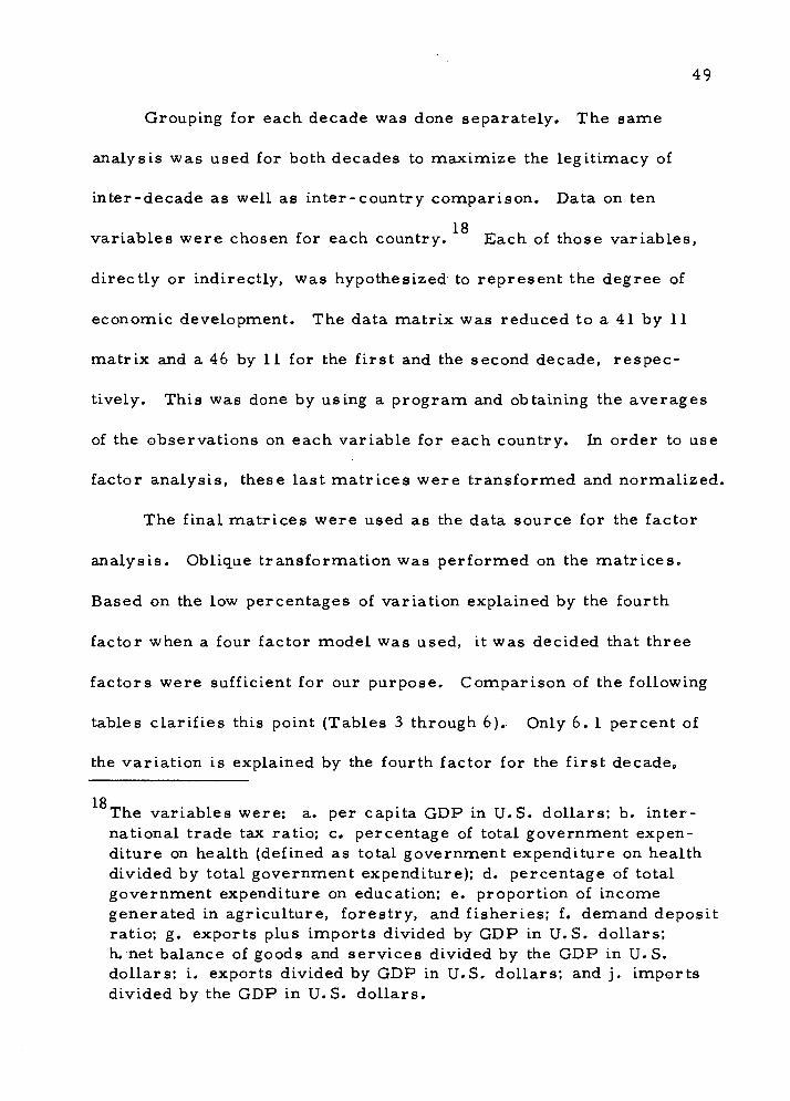
49
Grouping for each decade was done separately. The same
analysis was used for both decades to maximize the legitimacy of
inter-decade as well as inter-country comparison. Data on ten
18 variables were chosen for each country. Each of those variables,
directly or indirectly, was hypothesized to represent the degree of
economic development. The data matrix was reduced to a 41 by 11
matrix and a 46 by 11 for the first and the second decade, respec-
tively. This was done by using a program and obtaining the averages
of the observations on each variable for each country. In order to use
factor analysis, these last matrices were transformed and normalized.
The final matrices were used as the data source for the factor
analysis. Oblique transformation was performed on the matrices.
Based on the low percentages of variation explained by the fourth
factor when a four factor model was used, it was decided that three
factors were sufficient for our purpose. Comparison of the following
tables clarifies this point (Tables 3 through 6). Only 6. 1 percent of
the variation is explained by the fourth factor for the first decade.
18 The variables were: a. per capita GDP in U.S. dollars; b. inter- national trade tax ratio; c. percentage of total government expen- diture on health (defined as total government expenditure on health divided by total government expenditure); d. percentage of total government expenditure on education; e. proportion of income generated in agriculture, forestry, and fisheries; f. demand deposit ratio; g. exports plus imports divided by GDP in U.S. dollars; h. net balance of goods and services divided by the GDP in U.S. dollars; i. exports divided by GDP in U.S. dollars; and j. imports divided by the GDP in U.S. dollars.

50
Table 3. Cumulative percentages of three factors for the first decade.
Factor Eigenvalue Percent of variation
Cumulative percentage
1 2 3
17.195 13.137 7.887
45.0 34.4 20.6
45.0 79.4
100.0
Table 4. Cumulative percentages of four factors for the first decade.
Factor Eigenvalue Percent of Cumulative variation percentage
42.2 42.2 32.3 74.5 19.4 93.9 6. 1 100.0
1 2 3 4
17.195 13. 137 7.887 2.482
Table 5. Cumulative percentages of three factors for the second decade.
Factor Eigenvalue Percent of variation
Cumuli ative percen tage
44. .8 77. ,7
100, .0
1 2 3
16.842 12.368 8.375
44.8 32. 9 22.3
Table 6. Cumulative percentages of four factors for the second decade.
Factor, Eigenvalue Percent of variation
Cumulative percentage
1 16.918 38. 9 38.9 2 12.457 28.6 67.5 3 8.463 19.5 87.0 4 5.654 13.0 100.0

51
this figure is 13. 0 for the second decade. The following groups were
formed when the highest factor loading for each country was used
(Tables 7 and 8).
It was decided to divide the countries into three groups based on
the above factors. Factors F, and F^ formed the "underdeveloped 1+ 2+ ^
group" or group I, factors F and F formed the "developing
group" or group II, and factors F and F formed the "developed
group" or group III for the first decade.
There was one country, in the first decade, which in our judg-
ment, did not fall under the proper grouping. The highest loading for
Finland was on factor F , which constitutes part of our under-
developed group. Due to the given economic characteristics prevail-
ing in this country, it was decided to move it to the second group.
For the second decade, factor F, formed the underdeveloped 1+ v
group, factors F , F , and F formed the second group, and
factor F and F_ formed the group of developed countries. The
factor analysis results for the second decade were less definitive
than for the first decade. However, the subsequent classification did
not seem to contradict economic criteria.
Table 8 shows that Canada and France had their highest factor
loading on F with values of 0.621 and 0.688 respectively. It is
difficult to rationalize, on economic grounds, a change from
"developed" to "developing" for Canada. Thus, even though the factor

Table 7. Classification of the countries based on highest factor loading-- "first decade.
1 + 1- 2 + 3 +
Costa Rica Guatemala Chile India Phillipines F inland
South Africa Venezuela Austria Denmark Norway Switzerland New Zealand Netherlands
Egypt Ghana El Salvador Peru Burma Ceylon Iraq Syria Thailand Portugal
Canada U.S. France Sweden U.K. Australia
Brazil Colombia Ecuador Japan Turkey Italy Spain
Israel Jordan Lebanon Ireland
Table 8. Classification of the countries based on highest factor loading-- "second decade.
1 + 1- 2 + 2- 3 +
Egypt El Salvador Peru Ceylon Iraq Malaysia Syria Thailand Netherlands
South Africa U.S. Brazil Colombia Japan Italy Spain Australia New Zealand Venezuela
Canada Guatemala Burma India Philippines Turkey France
Kenya Dominican Rep. Israel Jordan Lebanon Ireland Portugal
Ghana Tanzania Costa Rica Chile Ecuador Iran
Austria Denmark Finland Norway Sweden U.K.
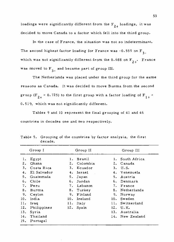
53
loadings were significantly different from the F_ loadings, it was
decided to move Canada to a factor which fell into the third group.
In the case of France, the situation was not so indeterminant.
The second highest factor loading for France was -0. 555 on F
which was not significantly different from the 0.688 on F . France
was moved to F and became part of group III.
The Netherlands was placed under the third group for the same
reasons as Canada. It was decided to move Burma from the second
group (F = 0.725) to the first group with a factor loading of F = L* T IT
0. 519, which was not significantly different.
Tables 9 and 10 represent the final grouping of 41 and 46
countries in decades one and two respectively.
Table 9. Grouping of the countries by factor analysis, the first decade.
Group I Group II Group III
1. Egypt 1. Brazil 1. South Africa 2. Ghana 2. Colombia 2. Canada 3. Costa Rica 3. Ecuador 3. U.S. 4. El Salvador 4. Israel 4. Venezuela 5. Guatemala 5. Japan 5. Austria 6. Chile 6. Jordan 6. Denmark 7. Peru 7. Lebanon 7. France 8. Burma 8. Turkey 8. Netherlands 9. Ceylon 9. Finland 9. Norway
10. India 10. Ireland 10. Sweden 11. Iraq 11. Italy 11. Switzerland 12. Philippines 12. Spain 12. U.K. 13. Syria 13. Australia 14. Thailand 14. New Zealand 15. Portugal
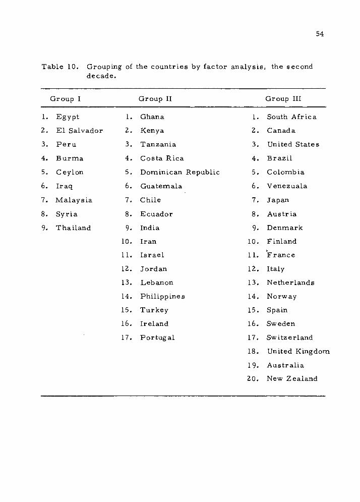
54
Table 10. Grouping of the countries by factor analysis, the second decade.
Group I Group II Group III
1. Egypt 1. Ghana 1. South Africa
2. El Salvador 2. Kenya 2. Canada
3. Peru 3. Tanzania 3. United States
4. Burma 4. Costa Rica 4. Brazil
5. Ceylon 5. Dominican Re spublic 5. Colombia
6. Iraq 6. Guatemala 6. Venezuala
7. Malaysia 7. Chile 7. Japan
8. Syria 8. Ecuador 8. Austria
9. Thailand 9. India 9. Denmark
10. Iran 10. Finland
11. Israel 11. France
12. Jordan 12. Italy
13. Lebanon 13. Netherlands
14. Philippines 14. Norway
15. Turkey 15. Spain
16. Ireland 16. Sweden
17. Portugal 17.
18.
19.
20.
Switzerland
United Kingdom
Australia
New Zealand
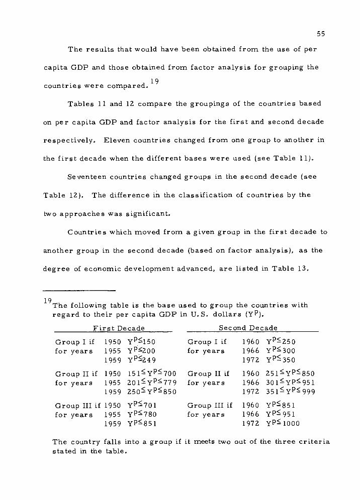
55
The results that would have been obtained from the use of per
capita GDP and those obtained from factor analysis for grouping the
A 19 countries were compared.
Tables 11 and 12 compare the groupings of the countries based
on per capita GDP and factor analysis for the first and second decade
respectively. Eleven countries changed from one group to another in
the first decade when the different bases were used (see Table 11).
Seventeen countries changed groups in the second decade (see
Table 12). The difference in the classification of countries by the
two approaches was significant.
Countries which moved from a given group in the first decade to
another group in the second decade (based on factor analysis), as the
degree of economic development advanced, are listed in Table 13.
19 The following table is the base used to group the countries with regard to their per capita GDP in U.S. dollars (Y^).
First Decade Second Decade
Group I if 1950 YP^150 Group I if I960 YP^250 for years 1955 Yp^200 for years 1966 Yp^300
1959 Yp^249 1972 Yp-350
Group II if 1950 151^Yp-700 Group II if I960 251^Yp-850 for years 1955 201^YP^779 for years 1966 301^YP^951
1959 250-Yp^850 1972 351-YP^999
Group III if 1950 Yp^701 Group III if I960 YP^851 for years 1955 Yp^780 for years 1966 Yp^951
1959 YP^851 1972 Yp^1000
The country falls into a group if it meets two out of the three criteria stated in the table.
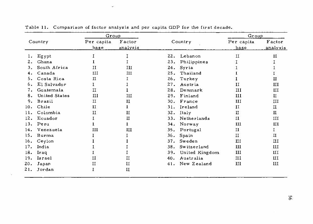
Table 11. Comparison of factor analysis and per capita GDP for the first deca tde.
•untry Group
Country Group
Cc Per cap ita F actor Per capita Factor base analysis base analysis
1. Egypt I J 22. Lebanon II II 2. Ghana I I 23. Philippines I I 3. South Africa II III 24. Syria I I 4. Canada III III 25. Thailand I I 5. Costa Rica II I 26. Turkey I II 6. El Salvador I I 27. Austria II III 7. Guatemala II I 28. Denmark III III 8. United States III III 29. Finland III II 9. Brazil II II 30. France III III
10. Chile II I 31. Ireland II II 11. Colombia II II 32. Italy H II 12. Ecuador I II 33. Netherlands II III 13. Peru I I 34. Norway III III 14. Venezuela III III 35. Portugal II I 15. Burma I I 36. Spain II II 16. Ceylon I I 37. Sweden III HI 17. India I I 38. Switzerland III III 18. Iraq I I 39. United Kingdom III III
19. Israel II II 40. Australia III III 20. Japan II II 41. New Zealand III III 21. Jordan I II
U1

Table 12. Comparison of factor analysis and per capita GDP for the second decade.
Group Country Per capita Factor
base analysis
Group Country Per capita
base Factor analysis
1. Egypt I I 2. Ghana I II 3. Kenya I II 4. South Africa II III 5. Tanzania I II 6. Canada III III 7. Costa Rica II II 8. Dominican Rep. I II 9. El Salvador I I
10. Guatemala II II 11. United States III III 12. Brazil II III 13. Chile II II 14. Colombia II III 15. Ecuador I II 16. Peru II I 17. Venezuela III III 18. Burma I I 19. Ceylon I I 20. India I II 21. Iran I II 22. Iraq I I 23. Israel III II
24. Japan III 25. Jordan I 26. Lebanon II 27. Malaysia II 28. Philippines I 29. Syria I 30. Thailand I 31. Turkey II 32. Austria III 33. Denmark III 34. Finland III 35. Netherlands III 36. Ireland III 37. Italy III 38. France III 39. Norway III 40. Portugal II 41. Spain II 42. Sweden III 43. Switzerland III 44. United Kingdom III 45. Australia HI 46. New Zealand III
III II II I II I I II III III III III II III III III II III III III III III III
-vl
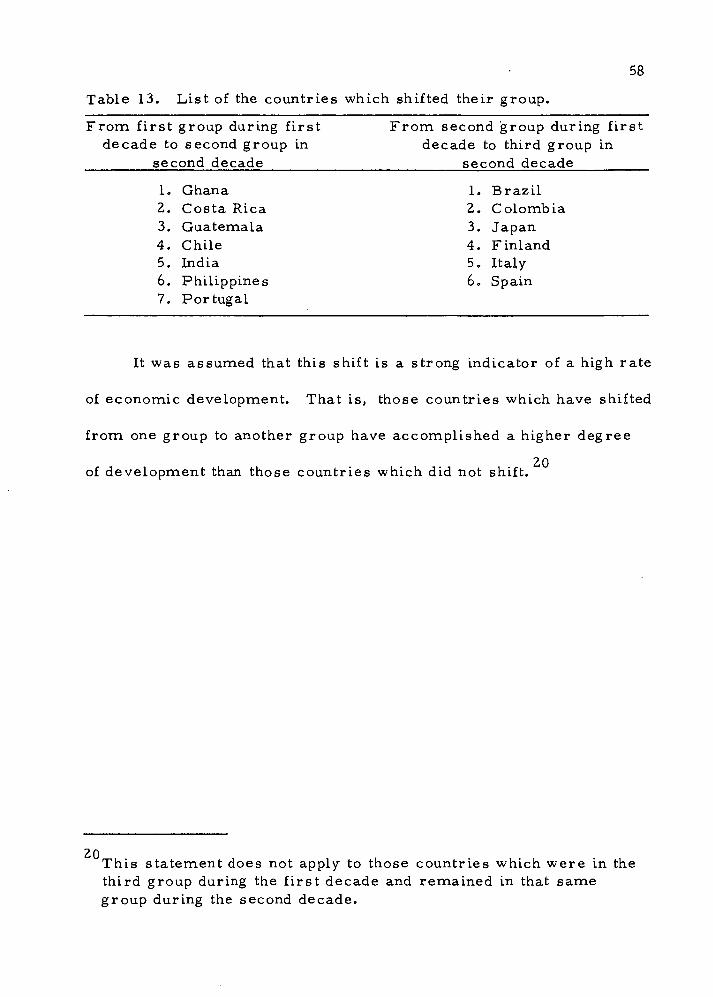
58
Table 13. List of the countries which shifted their group.
From first group during first decade to second group in
second decade
From second group during first decade to third group in
second decade
1. Ghana 2. Costa Rica 3. Guatemala 4. Chile 5. India 6. Philippines 7. Portugal
1. Brazil 2. Colombia 3. Japan 4. Finland 5. Italy 6. Spain
It was assumed that this shift is a strong indicator of a high rate
of economic development. That is, those countries which have shifted
from one group to another group have accomplished a higher degree
20 of development than those countries which did not shift.
20 This statement does not apply to those countries which were in the third group during the first decade and remained in that same group during the second decade.

59
V. METHODOLOGY AND TESTING THE HYPOTHESES
Total Tax Ratio
The models in this chapter deal with total tax ratio (TR). The
main obiective was to find the "best" models for explaining .total .tax
changes during the course of economic development. A priori formu-
lations of the best economic explanations were tested by selected
statistical techniques.
The analysis was designed to test the first hypothesis, 1) that
th££e_ij^_a^|rectjrelations,h^p_between the,djegx„ag„Qf.„§,cjQnp.rnric deyelop-
mei^_a^jyT!tgJtoiaI.„tajcJ_r„atio (TR), and 1-a) that this relationship
holds equally between a group of developed and less developed
countries as a whole as well as within a group of underdeveloped and
within a group of developing and/or developed countries.
It was hypothesized that the total tax ratio could have been
significantly affected by the six variables selected to reflect the
degree of economic development. Ordinary least squares (OL.S) was
used to estimate the parameters involved in the generalized linear
regression models (cf. Kmenta, 1971, Chapters 7, 10, and 12).
The following relationship was postulated.
TRit = bl<X it, 1)+ VYP it, 2)+ b3(OP it,3)+ VTPR it, 4)
-b5(ERit,5)-b6<ARit,6)+b7(DDRit,7)

60
where
i = 1,2, „ . ., N (number of countries, depending upon the group or groups of the countries in the model),
t = 1, 2, . . . , T (number of years, depending on the decade being analyzed),
TR = total tax ratio,
X = a dummy variable to assume a value of one throughout,
YP = per capita GDP in U.S. dollars,
OP = openness,
TPR = transfer payment ratio,
ER = ratio of expenditure on education,
AR = proportion of income generated in agriculture, forestry, and fisheries,
DDR = demand deposit ratio.
To enable making comparisons among different models possible,
the same variables were used in all the models whether statistically
significant or not in a particular model. Table 14 summarizes the
results obtained from the multiple linear regression analysis for
different groups of countries at different points in time.
The results of three sets of regressions are reported in
Table 14. The first set of regressions present the results obtained
using ordinary least squares (see Table 14a). Since time series data
21 were used, the regressions were tested for autoregression.
21 The existence of an autoregressive disturbance violates one of the OLS assumptions. It implies that the disturbance at one point of observation is correlated with other disturbances. This means

Table 14. Summary table of regression analyses for total tax ratio (TR).
a. The model R
Constant Y* OP TPR ER AR DDR
Durbin- Watson
St.
All countries, . 106 first decade (.012)
All countries, . 141 second decade (. 0097)
First group, .122 both decades (.0123)
First group, . 0906 first decade (.016)
First group, .116 second decade (.0193)
Second group, .0123 both decades (.0136)
Second group, -.017 first decade (.0286)
Second group, . 0272 second decade (. 0159)
Third group, . 192 both decades (.011)
Third group, .0164 first decade (.0176)
Third group, . 0226 second decade (.0141)
First S third groups, . 152 both decades (. 0083)
.000044** (.0000055)
.0000277** (.0000021)
-.000145** (.0000303)
-.00014** (. 00003)
.000081X
(.000053)
.000086** (. 00000709)
.000126** (.0000147)
.0000715**
(.0000083)
.000027** (.00000271)
. 0000228* (. 0000092)
.000024** (. 0000026)
.0000276** (.00000205)
.119** (.0122)
.139** (. 0099)
.151** (.0111)
.202** (.0154)
.087** (.015)
.0808** (.0149)
.0708** (.0174)
.0806**
(. 0247)
.113** (.0118)
.024 (.0229)
.116** (.0166)
.135** (. 0086)
.204**
(. 0206)
. 13** (.0144)
. 184** (.0201)
.103** (.0235)
.118** (.03)
. 0857** (.0151)
o .063
(.029)
.0872** (.0193)
. 15** (.021)
.364** (.0431)
.0845** (.0229)
. 18** (.0151)
-.109* (.0465)
-.15** (.0261)
-. 138**
(. 044)
-. 0656 (.0557)
-.533**
(.077)
.019 (.0308)
.0209° (. 0974)
-. 0663X
(.0418)
-.158** (.03)
-. 19** (.0601)
-.0132** (.0361)
-. 189** (. 0249)
-.0306 (. 0229)
-.0734** (.0177)
-.11** (.0267)
-. 141** (.0284)
.0403
(.047)
.0121 (. 0207)
.0357 (.0412)
. 00545
(. 0244)
-. 0723+
(.0446)
.052 (. 103)
-.168** (.0477)
-. 07** (.016)
-.108** .0135)
-. 109** .0112)
.0104 . 0164)
.0416* .0168)
.0606* .0272)
.0378° .0183)
.027 .0341)
.0518° .0237)
-. 178** .0126)
-. 154** . 0229)
-. 194** .0151)
-. 135** (. 00918)
, 615** 76.39** . 253
,630** 145.3** . 177
,572** 39.18** .468
,763** 45.71** 1.02
, 669** 28. 31** . 632
, 658** 86.46** . 282
,768** 46.42** .456
, 657** 57.23** . 274
,633** 99.27** .181
,701** 40.6** . 76
,711** 96.18** .169
.632** 151** .217
.88
,92
.82
,622
.76
.84
.724
.87
,92
.83
.92
,90
o
(Continued on next page)
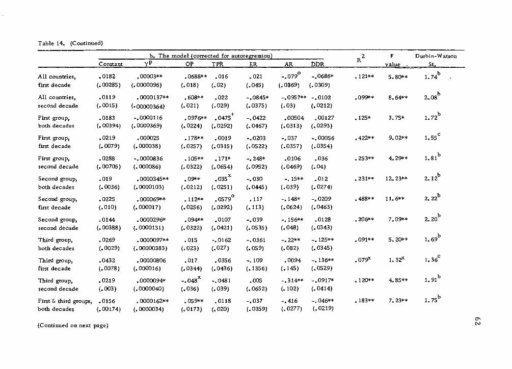
Table 14. (Continued)
b. The model (corrected for autoregression) Constant yP OP TPR ER AR DDR
All countries, .0182 .00003** .0688** .016 .021 -.079° -.0686*
first decade (.00285) (. 0000096) (.018) (.02) (.045) (. 0369) (. 0309)
All countries, .0119 .0000137** .608** .022 -.0845* -.0957** -.0102 second decade (.0015) (•00000364) (.021) (.029) (.0375) (.03) (.0212)
First group, .0183 -.0000116 .0976** .0475+ -. 0422 .00504 .00127 both decades (. 00394) (. 0000369) (. 0224) (.0292) (.0467) (.0313) (.0293)
First group, .0219 .000025 .178** .0019 -.0203 -.037 -.00056 first decade (. 0079) (.000038) (.0257) (.0315) (.0522) (.0357) (. 0354)
First group, .0288 -.0000836 .105** .171* -.248* .0106 .036 second decade (.00705) (. 000086) (.0322) (.0654) (.0952) (.0469) (.04)
Second group, .019 .0000345** .09** .035X -.030 -. 15** .012 both decades (. 0036) (.0000103) (.0212) (.0251) (.0445) (.039) (. 0274)
Second group, .0225 .000069** .112** .0579° .117 -.148* -. 0209
first decade (.010) (.000017) (.0256) (.0292) (.113) (.0624) (. 0463)
Second group, .0144 .0000296* .094** .0107 -.039 -. 156** .0128 second decade (.00388) (.0000131) (.0322) (.0421) (.0535) (.048) (. 0343)
Third group, .0269 .0000097** .015 -.0162 -.0361 -. 22** -.125** both decades (.0029) (.00000383) (.023) (.027) (.059) (.082) (.0345)
Third group, .0432 .00000806 .017 .0356 -.109 .0094 -. 136** first decade (.0078) (.000016) (.0344) (.0436) (. 1356) (. 145) (.0529)
Third group, .0219 .0000094* -.048X -.0481 .005 -.314** -.0917* second decade (.003) (.0000040) (.036) (.039) (.0652) (. 102) (.0414)
First & third groups, .0156 .0000162** .059*=* .0118 -.037 -.416 -. 046** both decades (.00174) (. 0000034) (.0173) (. 020) (.0359) (. 0277) (.0219)
R value ..
Durbin-Watson
St..
121** 5.80** 1.74
, 099** 8.64** 2.08
125* 3.75* 1.72
, 422** 9.02** 1.55
,253** 4.29** 1.81
,231** 12.23** 2.12
,488** 11.6** 2.22
, 206** 7.09** 2.20
, 091** 5.20** 1.69
>079x 1.32x 1.36
120** 4.85** 1.91
183** 7.23** 1.75
(Continued on next page)

Table 14. (Continued)
c. The best model Constant yP OP TPR ER AR DDR
R value
Durbin-Watson St.
All countries, first decade
All countries, second decade
First group, both decades
First group, first decade
First group, second decade
Second group, both decades
Second group, first decade
Second group, second decade
Third group, both decades
Third group, first decade
Third group, second decade
.0187 (. 0028)
.0117 (.00123)
.0169 (.00215)
.021 (.00617)
.027
(.0048)
.017 (.00258)
.0216 (. 0059)
.0145 (.0028)
.0266 (.0026)
.0426 (.0059)
.0210 (.003)
.00003** (. 0000096)
.0000138** (. 00000357)
.0000236 (.0000295)
.000035** (.0000102)
.0000717** (.0000166)
.0000303* (.0000129)
.0000091* (.00000376)
.0000033 (.0000138)
.0000093** (. 000004)
.069**
(.018)
.06** (.0208)
.096** .0471° (.0219) (.0283)
.178** (. 024)
.104** .211** (.0289) (.055)
. 091** . 035X
(.021) (.025)
.113** .0613° (.025) (.028)
. 101** (.0311)
-.045r (.0351)
.0268 (.0418)
-.075° -.069* (.0365 ) (.0308)
-.085* -.0936** (. 0374) (.0296)
-. 255** (.0914)
-.0396 (.0336)
-. 155** (. 0384)
-.151* (.061)
-. 164** (.0468)
-.226** -.0124** (.0814) (.0343)
-. 122* (. 0484)
-.311** -.092* (.101) . (.0413)
.118** 8.52** 1.74D
,098** 12.77** 2.08
120** 10.96** 1.71
,421** 18.68** 1.55
,237** 8.21** 1.85
, 229** 18.29** 2.12
, 480** 17.37** 2.22
, 203** 14.13** 2.20
. 086** 10.05** 1.68
, 071+ 2.43 1.36°
.113** 6.91** 1.90
** Significant at the 99 percent level Significant at the 97.5 percent level Significant at the 95 percent level Significant at the 90 percent level Significant at the 80 percent level
Do not reject the hypothesis that the autoregression is present at the 99 percent confidence level. Reject the hypothesis that autoregression is present at the 99 percent confidence level. The Durbin-Watson Statistic is inconclusive.
Figures in parentheses are the standard error of the regression coefficients. oo

64
22 Based on the Durbin-Watson Statistic for all the models it
was not possible to reject the hypothesis that autoregression was
present.
Out of the different kinds of procedures suggested for correcting
23 autoregression, the Durbin approach was used. The following
that when observations are made over time, the effect of the dis- turbance occurring at one period carries over into another period. It follows that autoregression, if not corrected for, results in inefficient regression coefficients, if OLS method is used (see Kmenta 1971, pp. 269-97).
22 Durbin-Watson Statistic was calculated as follows:
n 7
t=2 t t" * d =
n 2 2 e^ t=l t
where d is Durbin-Watson Statistic, e residual, and t represents time.
23 Assuming a univariate regression model as
Y = a + b Xl + e (A)
where Y. = dependent variable, a = intercept, b = slope, X1 = independent variable, e = disturbance term, if autoregression is present, two steps are followed. First, we write A as
Yt = a(l-p) + pYt_1 +bX1 - hpXt_1 + vt
Yt = a*+PYt_1+bXt + gXt_1+vt
This expression can be treated as a regression equation with three explanatory variables, Xt, X.,, and Y. _ ,, and estimated by OLS method. The resulting estimator of p, say p, is to be used to con- struct new variables (Yt - "pY._,) and (X. - pX._,). In the second step, we estimate
(Yt - "pYt_ j) = a* + b(Xt - Xt_ j) + v* , where a* = a(l- p). The estimators of a and b that are obtained using this approach are believed to have the same asymptotic properties as the maximum likelihood estimator. This approach is directly applicable to a generalized regression model with pooled cross-section, time- series data, such as those used here (see Kmenta 1971, p. 289).
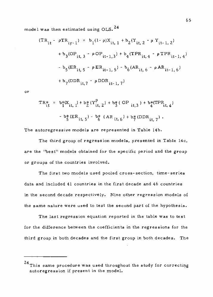
65
24 model was then estimated using OLS.
<TRit- ""Vl) '- bl(1-p)Xit,l+b2(Yit,2-PYit-l(2)
+ b3(OP.tj3 - POPit.1;3) +b4(TPR.t)4 - pTPR.t_li4)
-b5(ER.t)5-pER.t_1)5)-b6(AR.t)6-pAR.t_1)6)
+ b (DDR - pDDR ) 7 it, 7 it- 1, 7
or
TR* = b*(X. ) + b*(YP ^)+b*(OP. , ) + b*(TPR ) It 1 It, 1 2 it, Z' 3 v it,3 ' 4 it, 4
- b*(ER.. .) - b* (AR .. ,) + b*(DDR.t \ . 5 it, 5 6 it, 6 7 it, 7
The autoregressive models are represented in Table 14b.
The third group of regression models, presented In Table 14c,
are the "best" models obtained for the specific period and the group
or groups of the countries involved.
The first two models used pooled cross-section, time-series
data and Included 41 countries in the first decade and 46 countries
In the second decade respectively. Nine other regression models of
the same nature were used to test the second part of the hypothesis.
The last regression equation reported In the table was to test
for the difference between the coefficients In the regressions for the
third group In both decades and the first group In both decades. The
24 This same procedure was used throughout the study for correcting autoregression if present in the model.

66
null hypothesis was formulated as
H : No difference between the regression coefficients of the o
two groups.
25 26 Chow test statistic was used and the F value obtained was 2.75.
Since the critical value for F (7,463) at the 99 percent level of con-
fidence is 2.64, we see that the null hypothesis cannot be accepted.
Interpreting the Results
The regression results obtained from analyzing the data for
41 countries, for the period 1950-5 9, strongly support our general
27 hypothesis. All the variables, with the exception of DDR, carry
the expected signs, and all but ER and TPR are significant. The
best model excludes TPR and ER. All the variables in this model are
25 Chow Statistic is defined as
(SSEJ - (SSE^, + SSE ))/k _ d+u d u
(SSEj + SSE )/N - 2k d u
where SSes are sums of squares for error term, d is the group of developed countries, u the group of underdeveloped countries, k is the number of variables in the model, and N is the number of observations in both models (d and u) (see Chow I960, pp. 591-605).
26Using the formula in footnote 25 we have _ (.0948) - (.05609 + .03493))/7 _
F= (.090871)7463 -L.i*.
27 The following countries were excluded from this analysis due to the lack of data on one or more variables: El Salvador, Iraq, Lebanon, Philippines, Thailand, Turkey, Sweden, Switzerland, and France.

67
significant and carry the expected sign except DDR, as in the original
model. The negative sign for DDR is attributed to the inclusion of
developed countries in the model. The only significant variable for
the group of developed countries was DDR with a negative sign. This
is not surprising as it is only possible to have credit cards and credit
unions involved in transactions if the economy, its financial institu-
tions and appropriate administration are developed. The sign for
DDR is also negative for the other two groups in this period, but the
sign is statistically insignificant in both cases. This, however,
reinforces the sign for DDR to become negative when all the groups
are pooled together.
The use of data from the second decade for 46 countries again
28 provided strong support for the general hypothesis. All the vari-
ables but DDR carry the expected signs. DDR was dropped out when
the best model was selected. All of the signs are as expected and
variables in the best model are significant.
The results obtained from the second decade are more reliable
because; (1) the data are expected to be more accurate, and (2) there
are more sample countries with longer time periods. However, both
models support the hypothesis and offer per capita GDP; proportion
of income generated in agriculture, forestry, and fisheries; openness;
28 Iraq, Lebanon, Turkey, and Switzerland are excluded from this analysis.

68
ratio of expenditure on education; and demand deposit ratio; as the
variables most closely related to total tax ratio changes as the
economy develops.
In order to determine whether a strong relationship exists
between the degree of economic development and total tax ratio for
the group of underdeveloped countries, data from the first group of
29 countries in both decades were used. All of the variables in the
model except AR and Y have the hypothesized signs, with OP and
TPR being significant. The model for the period 1950-1972 supports
the hypothesis that the specified relationship does exist among the
group of underdeveloped countries considered by themselves. Per
capita GDP did not remain in the model when the best model was
sought, neither did ER, AR, and DDR. This result supports the
conclusion arrived at by Hinrichs (1966), i.e., openness, not per
capita income, explains the total tax ratio changes in underdeveloped
countries. Besides OP, TPR plays an important role in explaining
such changes.
When the data for the group of underdeveloped countries, in the
first decade, were used, the result still supported the specified
hypothesis. The same was true for the first group in the second
decade.
29 El Salvador, Iraq, Philippines, and Thailand were excluded from the analysis due to the lack of data on one or more variables.

69
OP, TPR and ER have played an.important role in explaining
tax ratio changes during the recent years. Their presence in the
best model for the second decade supports this point. The positive
sign for AR in the second decade was not significant. DDR did not
remain^in either of the two models.
Openness remains the predominant explanatory variable for both
decades along with TPR which gains importance during the second
decade. The significance of OP appearing in the models for under-
developed countries is not only because these countries rely heavily
upon trade taxes, but because openness itself is an indicator of the
degree of economic development. Underdeveloped countries typically
need to increase their imports of capital goods and other services to
foster their development projects. Exports are needed to provide
them with foreign exchange.
The results obtained from the regression analysis for the
second group in both decades provide evidence that for the group of
developing countries the tax ratio is strongly related to the degree of
30 economic development. All of the variables in the model carry the
expected sign. Only ER and DDR are not significant, and drop out of
the best model. Per capita GDP along with openness and proportion
of income generated in agriculture constitute the most significant
30 Turkey and Lebanon are not included here in this analysis.

70
variables. All three are significant at the 99 percent level of confi-
dence. TPR remains in the model at 80 percent level of confidence.
When the data from the developing countries in the first decade
31 were used the result was equally satisfactory. The same was true
32 of this group for the second decade.
In general, for the group of developing countries, Y , OP, and
AR are associated with tax ratio changes during the course of econo-
mic development. TPR appears in the best model for the first decade
and the one for both decades. The emergence of per capita GDP, at
this stage of development, as a factor for explaining tax ratio
changes, is an indication of the fact that collection of other taxes
33 rather than traditional trade taxes becomes feasible. Openness
and AR remain as the other two dominant factors, demonstrating that
no single factor explains tax ratio changes at this level of economic
development but rather three and in some cases four, if TPR is
included. The models taken as a whole tend to substantiate the basic
hypothesis in this section.
31 With Turkey and Lebanon excluded.
32 With Turkey and Lebanon excluded.
33 This does not necessarily imply that all the countries in this group have increased their tax revenue through other sources rather than trade taxes. As it will be shown there are a limited number of countries that have taken advantage of this opportunity to improve their tax revenues.

71
The group of developed countries was also examined, When the
data from both decades were used, the hypothesis of a direct rela-
.'3
tionship between total tax. ratio changes and the degree of economic
34 p development could not be rejected. Y , AR, and DDR play the
dominant role in explaining such changes for the group of developed
countries. A negative sign for TPR was observed but the coefficient
was not statistically significant. The best model includes Y , AR,
and DDR with the expected signs. The negative sign for DDR is not
contrary to the hypothesis regarding the decrease in its relative
importance due to the development of other substitutes, as the
medium of exchange, such as credit cards, etc. , which is only
possible when the country is highly developed. AR and DDR are
significant at the 99 percent confidence level, while Y is significant
at the 97.5 percent confidence level. The importance of Y in
explaining tax changes for this group of countries was highly empha-
sized in past studies. However, when the data for the first decade
for the group of developed countries were examined, this emphasis
did not seem to be convincing. As the results showed, the only
variable which could have remained statistically significant was DDR.
In other words, none of the explanatory variables was statistically
significant but DDR. AR did not carry the hypothesized sign, although
34 The analysis excludes Sweden, Switzerland, and France from the first decade and Switzerland from the second decade due to lack of information on one or another variable.

72
it was not significant. The F test for the whole model was signifi-
cant only at the 80 percent confidence level. The best model would
have included only DDR. However, Y and TPR were kept in the
model for analytical reasons. TPR was significant at the 50 percent
confidence level, the best variable after DDR. Y was kept in the
model in order to show to what extent past studies have overempha-
sized its importance in explaining tax changes for developed coun-
tries in that period. The comparison is possible because the period
covered is approximately comparable to that of past studies, except
for Chelliah's (1971). Additional analysis was required due to the
significant difference between the results obtained from the data in
the second decade for the developed countries.
The result from the third group in the second decade, showed
that our hypothesis strongly holds for this group during the second
decade. Y , in this period, does explain a good part of the tax ratio
changes occurring with economic development. AR, DDR, and OP
were also statistically significant variables with the right sign except
for OP which carries a negative sign. This indicates that although
the total tax ratio increases during economic development, the
reliance on trade taxes is diminishing. All of the variables, but TPR
and ER, did stay in when the best model was selected. In this best
model Y and AR were significant at the 99 percent confidence level,
73
while DDR and OP were significant at the 97.5 and 90 percent level
respectively.
The sharp difference between the results obtained for the first
decade and the second decade raised some serious questions. Also
the implication of the results obtained for the first decade seemed
curious. It was felt that a more extensive analysis was required
before any generalization could be made.
In order to accomplish this, those countries which were
included in the third group during the first decade were examined
separately during the second decade. A regression, identical to the
one used for the data from the first decade, was run, using second
decade data. This was done in order to extract any influence that
the group of countries which shifted from second group in the first
decade to the third group in the second decade might have had on the
results obtained from analyzing the third group in the second decade.
An appropriate F statistic was obtained to test the hypothesis that the
inclusion of shifted countries in the third group for the 1960-73
period had significantly affected the results for this group. The
result was not significantly different from the third group result
35 when the shifted countries were included.
35 The test employed was the familiar Chow test
(SSEr - SSEJ/m F = f d
SSEJ/(n-k) d
where SSE denotes the sum of squared residuals, f represents the

74
The conclusion is that other factors besides the degree of
economic development (expressed by per capita income or GDP in
the past studies) have been responsible for changes in the total tax
36 ratio for the group of developed countries in the 1950-59 period.
Identification of these factors by themselves require indepth analysis,
perhaps mostly historical and/or subjective in nature. However,
three explanations could be provided; (1) during the 1950's, more
importance was placed on fiscal policy as a means of correcting for
business cycles and stabilization. Consequently, tax changes were
due to economic policy factors rather than economic development as
these countries were already highly developed and could have used
any type of taxes they desired in order to increase their tax
revenue and thus tax ratio. But at times, reduction of the tax ratio
for correcting unfavorable changes in the economy was required (OECD
1968 , Chapters II and III). (2) Democracy and political campaigning
exist in these countries. Tax change is, or at least has been, the
whole sample countries, d represents only those countries which did not shift, m is the number of observations for the countries which shifted, n the number of observations for those which did not shift, and k is the number of independent variables. The F value for Chow Test Statistic was 0.447. Since the critical value of F(53, 146) at the 99 percent level is 1.50, the null hypothesis of an equal regression coefficient in the two regressions could not be rejected.
36 The relatively high degree of variation in the tax ratio may have been responsible for the appearance of such coefficients in the model. Statistically speaking, such variation may have resulted in a downward bias in the regression coefficients.
75
predominant factor in presidential and other types of campaigns and
political elections. Thus politics have had something to do with
taxes. This means in a country such as U.S. where they have an
election every four years, it is always possible to have tax changes
if the party is changed. In fact this has happened even in cases
where the same party won the election or during the time that the
same president has been in office. (3) The countries were already
developed and merely took advantage of their high degree of develop-
ment by using many types of available taxes for increasing revenue.
They did not need any further degree of economic development to
37 enable them to impose higher taxes.
Surprisingly, the results from the second decade did not show
this to be the case during that period. Based on the rising importance
of the public sector in the economy, higher taxes were needed.
Politicians, along with political economists, looked for alternative
taxes to replace those taxes whose impacts were reflected directly
on consumers. Politicians of these countries tried to use taxes
which are not visible to the public in order to reduce other kinds of
taxes (direct) to win public support. Indirect taxes do result in
higher prices. It is, and has been, easy for the politician in these
countries to blame higher prices on "unknown forces causing
37 This statement did not hold for the same group during the second decade due to the increase in government participation in economic activities and, thus the growth of the public sector.

76
inflation." Tax innovation, i.e., formulation of new tax sources,
followed this trend and resulted in higher tax ratios as the economy
developed. This is supported by the results obtained from analyzing
the trend of indirect taxes during the second decade for the groups of
highly developed countries.
A significant difference between the coefficients of the regres-
sion models for the developed and underdeveloped countries was
observed. The general models using data for 1950-1972 period did
confirm that a direct relationship does exist between the degree of
economic development and total tax ratio for the group of under-
developed and developed countries, each analyzed separately. It was
concluded that specific development factors or variables were
responsible for the significant difference between the two regression
models. It was necessary to identify those variables. A test of the
difference between the coefficient of each individual variable provided
38 the answer.
38 The test statistic used was
t = b - b.
id m
(S )2 + (S )2
a u where i = 1, 2, . . . , 6 corresponding to the independent variables, d denotes developed countries, u denotes underdeveloped countries, b is the coefficient for the independent variable, S is the estimated standard error of regression coefficient, with n + n, degrees of freedom, n corresponds to the number of observations in each group of countries.
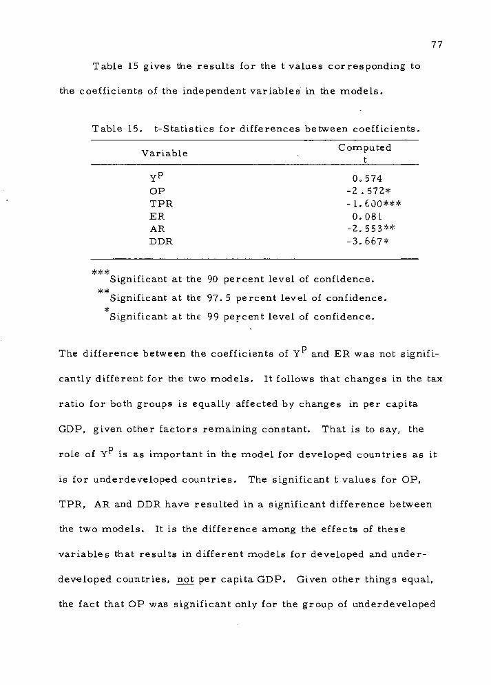
77
Table 15 gives the results for the t values corresponding to
the coefficients of the independent variables in the models.
Table 15. t-Statistics for differences between coefficients.
... Computed Variable
YP 0.574 OP -2.572* TPR -1.600*** ER 0.081 AR -2.553** DDR -3.667*
*** Significant at the 90 percent level of confidence.
** Significant at the 97. 5 percent level of confidence.
* Significant at the 99 percent level of confidence.
The difference between the coefficients of Y and ER was not signifi-
cantly different for the two models. It follows that changes in the tax
ratio for both groups is equally affected by changes in per capita
GDP, given other factors remaining constant. That is to say, the
role of Y is as important in the model for developed countries as it
is for underdeveloped countries. The significant t values for OP,
TPR, AR and DDR have resulted in a significant difference between
the two models. It is the difference among the effects of these
variables that results in different models for developed and under-
developed countries, not per capita GDP. Given other things equal,
the fact that OP was significant only for the group of underdeveloped
78
countries supports the idea that underdeveloped countries relied
heavily on trade taxes.
Conclusions and Generalization
The following conclusions and generalization are made based
upon the results obtained for this section.
1. The general theory of a direct relationship between total
tax ratio and the degree of economic development is maintained. That
is, the more developed the country the more taxes it collects relative
to its^GrDP. This hypothesis holds for the group of underdeveloped
countries as well as developed and/or developing countries.
2. Openness is the variable best explaining the degree of
development and is the one most closely related to tax ratio changes
in underdeveloped countries. This led to the conclusion that the
group of underdeveloped countries rely heavily upon trade taxes.
Appearance of openness and its significance along with TPR and ER
supports the hypothesis that the degree of economic development has
affected the total tax ratio even in underdeveloped countries, espe-
cially during the 1960-1972 period.
3. Statistically speaking, the most reliable models are those
of the second group—developing countries. These models have the
highest power in relating tax ratio changes to the degree of economic
development.

79
4. The appearance of Y , besides OP, as a significant variable
in the models for the group of developing countries, may be considered
as evidence that it is at this stage of development that the government
is able to rely on sources of taxation other than trade taxes. In other
words collection of other kinds of taxes becomes feasible at this
stage of development, be it direct or indirect.
5. The general hypothesis is maintained for the group of
developed countries. However, there is no hard evidence that factors
indicating the degree of economic development can fully explain the
total tax ratio changes for this group during the 1950-1959 period. It
is suspected that besides the degree of economic development, other
factors such as politics and role of fiscal policy in stabilization
practices have also been responsible for the variations in total tax
ratio, especially during the first decade.
6. Inclusion of the countries which shifted from the second
group in the first decade to the third group in the second decade did
not have a significant effect on the results obtained for the group of
developed countries during the 1960-1972 period.
7. Past studies have emphasized the importance of Y as a
variable for explaining tax changes for developed countries, espe-
cially during the 1950-1959 period. Given other things being equal,
the role of Y is equally as inaportant in explaining tax ratio changes
for underdeveloped countries.

80
Direct Tax Ratio
The models in this section deal with the relative importance of
direct taxes in total tax revenue. Tax components, gr-r,elativer
importance of special groups of taxes may be analyzed in terms of
either the percentage of different taxes in total.Jtax revenue or the
ratio of these taxes to GNP. Chelliah believes that the first alterna-
tive brings out more clearly the differences in the patterns of taxa-
tion between different countries, irrespective of the level of taxa-
39 tion (see Chelliah 1971, p. 267).
Tax components were analyzed in terms of the percentage of
direct taxes in total tax revenue. In order to perform such a func-
tion, it was hypothesized that as the economy develops the tax
structure of the country changes toward more intensive use of direct
taxes, i.e., the relative proportion of direct taxes in total tax revenue
tends to increase as the economy develops. It was decided to test the
hypothesis using long^run^data to ensure that a complete transition,
in terms of economic development, had occurred.
39 4.u If TR. is the yield of i"1 tax; TTR that of total taxes; Y = GDP, then TR^Y = TRL/TTR • TTR/Y. Hence TRjVY series is the TRj/TTR series weighted by TTR/Y ratio (cf. Chelliah 1971, p. 268).

81
postulated
To test this hypothesis, the following relationship was
40
T< = bl(Xit,l)+b2{YPit,2)+b3(OPit,3)+VTPRit,4)
-b5(ER.t(5)-b6(AR.t)6)+b7(DDR.t)7)
where
i = 1,2, ...,N (number of countries, depending upon the group or groups of the countries in the model),
t = 1, 2, . . . , T (number of years, depending on the decade being analyzed),
d TR = total tax ratio,
X = a dummy variable to assume a value of one throughout,
40 Originally the following relationship was postulated.
TRft = bl(Xit, 1> + V^.Z* + b3(TPRit, 3) " b4(ARit, 4)
+ VDDRit,5> + VEXit,6>- Where i - 1,2,.. .,N (number of countries depending upon the group or groups of countries in the model), t = 1, 2, . . ., T (number of years depending on the decade being analyzed), TRd = direct tax ratio, X = a dummy variable to assume a value of one throughout, YP = per capita GDP in U.S. dollars, TPR = transfer payment ratio, AR = proportion of income generated in agriculture, forestry,
and fisheries, DDR = demand deposit ratio, EX = exports in millions of U.S. dollars. A high degree of multicolinearity was observed between Y" and EX in some of the models which resulted in imprecise estimates of the regression coefficients. This imprecision arises because of the large variance of the least squares estimators (see Kmenta 1971, pp. 380-391). To avoid the violation of this basic assumption of OLS and maintain the comparability of the results, a similar model to the one used for total tax ratio was employed.

82
Y = per capita GDP in U.S. dollars,
OP = openness,
TPR = transfer payment ratio,
ER = ratio of expenditure on education,
AR = proportion of income generated in agriculture, forestry, and fisheries,
DDR = demand deposit ratio.
Openness was specifically included because of its relationship
to direct taxes emphasized by Hinrichs. He states;
. . . personal income taxes may be based primarily on civil servants. . ., the army. . ., and/or employees of the large mineral and/or export companies, especially foreign ones. Thus, the openness of the economy would normally affect the amount of personal income collected (1965, p. 556).
If this relationship was maintained, openness should have carried a
positive sign in the models. The first set of regressions in Table l6a
summarizes the results obtained from the multiple linear regression
analysis for different groups of countries at different points in time,
using OLS. The Durbin-Watson Statistic was calculated for these
models. It was not possible to reject the hypothesis that autore-
gression was present. The Durbin procedure was used to correct for
autor egress ion.
The second group of regression models presented in Table 16b
is the results of the original models corrected for autoregression.
The last set of regressions are the "best" models obtained for the

Table 16. Summary table of regression analyses for direct tax ratio (TR )„
a. The model R
Constant OP TPR ER AR DDR
F value
Durbin- Watson
St.
First decade, all countries
Second decade,
all countries
First group, both decades
First group, first decade
First group, second decade
Second group, both decades
Second group, first decade
Second group, second decade
Third group, both decades
Third group, first decade
Third group, second decade
.446
(. 0438)
.339 (.0376)
.427 (. 0549)
.432 (.069)
.452 (.089)
.0877 (.0511)
.151 (. 107)
.0699 (.0541)
.439 (.0486)
.503 (. 059)
.390 (.0714)
.000119** (.0000177)
. 0000427**
(. 00000873)
.00016>:
(.000133)
.000113 (.000185)
.000497° (.000244)
.0000826** (.0000265)
.0000532
(.000055)
.000145** (.0000283)
-.00000458 (.0000119)
-. 0000551+
(.0000312)
.00000246 (.0000134)
-. 0457
(.044)
-.132** (.0406)
-.104° (.047)
-.089 (.0895)
-.0177 (.0702)
-. 327**
(.0557)
-. 187** (.0651)
-.372**
(.0843)
.048 (.0518)
-. 149+
(.0775)
.0182 (.0841)
-. 206** (.0741)
-.0837x
(. 059)
-.249** (.088)
-. 662** (.139)
.386** (.137)
-.194** (.0566)
o -.224 (. 109)
-.218** (.0658)
.143X
(.0919)
.757** (. 146)
.0183 (.118)
-.560** (. 167)
.058 (. 107)
-. 434° (. 202)
-.065 (.351)
-.479X
(. 356)
.181X
(.115)
-1.198** (.365)
.684** (. 142)
-.503** (.132)
-. 339+
(. 204)
-.281X
(. 184)
. -. 39** (.082)
-.419** (. 072)
-.028 (.117)
-. 242x
(.166)
-.225 (.218)
-. 110X
(.0775)
.224X
(. 154)
-.144** (.0834)
-1.11**
(.195)
-2.18** (.348)
-1.03** (.242)
.206** (.047)
.282** (.0459)
-.0091 (.0728)
.114 (. 103)
-.432**
(. 125)
.655** (.0687)
1.12** (. 127)
.526** (.0808)
.364** (.055)
.545** (. 077)
.39**
(. 0769)
.529**
.403**
. 106**
.290**
. 232**
.358**
.600**
.431**
.231**
.535**
.219**
53.55** .155 ,91
57.57** .053a .98
3.46** . 202 .88
5.73** . 358 .86
4.24** .258 .81
25.08** -.106a .97
21.06** .272 .93
22.56** .137* .97
17.27** .067 .97
19.97** .48 .88
10.93** .031 .97
Continued on next page)
00

Table 16. (Continued)
b. The model (corrected for autoregression)
Constant YP OP TPR ER AR DDR
First decade, .0402 .0000611+ -.0455 -. 109+ -.109 .008 -.0134 all countries (.008) (.0000353) (. 0604) (. 0656) (. 184) (.131) (. 109)
Second decade, .00883 . 0000144X -.01741 -.0348 .078 .048 .116* all countries (.00199) (. 0000105) (. 0480) (.0702) (. 0857) (.0668) (. 0487)
First group, .0416 -. 0002741° .0478 -.130X -.141 .223° .0219 both decades (. 00905) (.00013) (.0821) (.095) (. 182) (. 102) (. 0976)
First group, .0429 -.000149 .151 -.208X -.225 .145 .0757 first decade (.0186) (.000178) (.133) (. 128) (. 268) (. 173) (. 197)
First group, .0529 -.000057 .0117 .174 .011 .171X -.146X
second decade (.0172) (.000261) (.099) (. 199) (. 268) (. 129) (.HI)
Second group, .0106 .0000538+ -.0119 -. 0491 .165+ -.187° .0542 both decades (. 00267) (. 0000297) (. 0446) (.0586) (.0952) (.0882) (.058)
Second group, .0352 -. 0000437 -. 135* -.0091 .44+ -.115 -.143 first decade (.0068) (. 000047) (.0577) (.066) (.243) (. 203) (.118)
Second group, .0085 .0000922* .0663 -.101 .133 -. 154x .iiox
second decade (. 0034) (. 0000369) (.066) (.102) (. 108) (.0995) (.069)
Third group, .019 . 00000367 -. 222** -.053 -.0407 -.107 .26° both decades (.0048) (.0000129) (.0675) (.0762) (.183) (. 243) (.116)
Third group, .0807 .0000277 -. 204+ -.0543 -.437 -.266 .0442 first decade (.0227) (. 0000606) (.115) (. 143) (.483) (.498) (. 222)
Third group, .011 .00000409 -.221* -.0148 .080 -.0484 .356** second decade (. 004) (.0000109) (.0911) (.0938) (.162) (.246) (. 104)
R F
value
Durbin- Watson
St.
,028
,020
,076
,097
.077'
,049
140
.084**
,05*
.067
,069*
1.22
1.63
2.13
1.29
1.07
2.11
1.99
2.50**
2.73*
1.11
2.64*
2.00
1.84
1.56
1.78
1.24
1.82
1.62
1.99
2.22
2.14
2.07
a
(Continued on next page) 00

Table 16. (Continued)
c. The best model R2 F
value Durbin-Watson
Constant YP OP TPR ER AR DDR St.
First decade, all countries
Second decade, all countries
First group, both decades
First group,
first decade
First group, second decade
Second group, both decades
Second group, first decade
Second group, second decade
Third group, both decades
Third group, first decade
.037 (.00428)
.00903 (.00189)
.0416 (.0063)
.429 (. 0084)
.0526 (.0109)
.0111 (. 00227)
.0319 (.00597)
.009 (. 003)
.0192 (. 00402)
.0869 .00909)
.0000632* (. 0000334)
.0000146X
(. 0000104)
-.000281* (. 000124)
.0000567 (.0000288)
.000087* (.000035)
Third group, .0124 second decade (.00312)
Significant at the 99 percent level Significant at the 97,5 percent level
0Significant at the 95 percent level Significant at the 90 percent level Significant at the 80 percent level
-. 109 (.0648)
-.124 (.0939)
+ o .195 -.236
(.121) (.115)
-.123 (.0545)
-. 224** (.0666)
o -.222
(. 108)
-. 223* (.0889)
-.491 (.435)
.222 (. 100)
. 024 3. 23
.113* .016* 3.91* (.0483)
. 071** 4. 03**
.073
.212* -.135x .063 (. 120) (. 100)
.172+ -. 192° .043*
(. 0937) (. 0879)
.483° -.172X .127*
(. 235) (.113)
-. 159X .120+ .072* (.099) (.068)
.264* . 047** (.116)
.059
. 357** . 067**
2.98
2.71
3.73*
3.68*
3.74*
7.-85**
3.01
7.84**
1.98
1.83
1.57
1.83
l^""
1.80
1.59^
1.90
2.21
2.11
2.08
aDo not reject the hypothesis that the autoregression is present at the 99 per-
cent confidence level. Reject the hypothesis that autoregression is present at the 99 percent level. cThe Durbin-Watson Statistic is inconclusive. Figures in parentheses are standard error of the regression coefficients.
00

86
specific period and the group of the countries involved and are
reported in Table 16c.
Two general models are reported in the table. The first one
used pooled cross-section, time-series data for 41 countries and
10 years. The second model used the same sort of data for 46
countries and 13 years. The rest of the regression equations were
estimated to find out if the specified relationships hold for different
41 groups of countries during the first and/or second decade.
Interpreting the Results
The results obtained from analyzing the data for 41 countries,
for the 1950-5 9 period, did not provide a promising answer to the
question posed. There were contradictory signs in the model. Per
capita GDP assumed a positive sign and was significant at the 90 per-
cent level of confidence. However, TPR, the only other significant
variable in the model, did not carry the expected sign, neither did
OP, AR, or DDR. The best model included YP and TPR, each sig-
nificant at the 90 percent confidence level, with opposite signs. It
was concluded that due to the sharp differences in the direction of
direct taxes at different stages of development during the first decade,
41 All those countries which were excluded from the analysis due to lack of data on one or another variable in the models for total tax ratio are also excluded from these analyses since the models used are identical in both investigations.

87
a general study of all the countries was not able to provide a satis-
factory explanation to the variation in direct tax ratio associated with
the degree of economic development.
The use of data from the second decade for 46 countries pro-
vided a better explanation for direct tax ratio changes. Although
some variables carried signs contrary to our a priori assumptions,
the best model selected did not include any of those variables. Per
capita GDP and DDR remained in the best model with the expected
signs. They are significant at the 80 percent and 97.5 percent level
of confidence, respectively. Based on the reliability of the data for
this period, it was concluded that during the second decade, the more
developed the country the more direct taxes were collected relative to
other sources of taxes. This held only when the group of developed
and developing and/or underdeveloped countries was combined. It
did not hold when each group was analyzed separately.
When the data from both decades were used for the group of
underdeveloped countries, it was strongly maintained that TR has
been decreasing during this period. With all the variables in the
model, only ER, OP and DDR had the expected sign to support the
general hypothesis. However, none were statistically significant.
When the best model was selected, variables such as Y , TPR, and
AR remained in the model, each being significant at the 97.5, 80, and
95 percent level of confidence, respectively. As the signs for these

88
variables indicate, TR not only did not increase, but it decreased as
their economy developed. This decrease was due to the reliance of
those countries on trade taxes, as was observed in the last section.
Obviously the decrease in TR did not result in decrease in TR. What
it showed was that the relative importance of direct taxes has been
decreasing in these countries and the relative share of trade taxes in
total tax revenue, and possibly other indirect taxes, has been increas-
ing during the last two decades. Some of these countries did in fact
use other indirect sources, during the first decade and shifted to the
second group in the second decade, a development stage where direct
42 tax collection not only becomes possible but is practiced.
Had it been possible for these countries to collect direct taxes,
they might have done so. Direct tax collection has been, and still is,
practically impossible for the countries at this stage of development.
Invariably it meets with serious administrative, political, and social
obstacles.43
42 Chelliah, analyzing the relationship between the share of direct taxes (TR ) and per capita income for 50 countries, using the data for 1966-68, finds the following regression equation:
TRd = 33.08 - 0.052(YP) . ^ 2 nnc
(5.575) (1.059) WlthanR =0-005
for the countries with per capita income below U.S. $200. Note; figures in parentheses are t-ratios (1971, p. 314).
43 These points were discussed, in the second chapter of this study.
89
The regression equation relating to the first group of countries
in the first decade was not as clear as when the data from both
decades were used. Y carried a negative sign and it was
not significant. The same was true for AR with
a positive sign. Given the full model, it was concluded that TR
dropped during the first decade for the group of underdeveloped
countries. The best model included OP with a positive sign and was
significant at the 80 percent level of confidence, along with TPR with
a negative sign and significance at the 95 percent level of confidence.
The negative sign for TPR reinforced our preceding conclusion. The
positive sign for OP during this period supports Hinrichs1 assertion
that underdeveloped countries may collect income taxes on import/
export companies, and the larger these companies get the higher the
income tax (direct) collected.
The results obtained from analyzing the data for underdeveloped
countries during the second decade strongly indicates that TR has
been decreasing for this group during 1960-1972 period.
Per capita GDP carried a negative sign along with DDR. The
latter was significant at the 80 percent level of confidence. OP and
TPR, with positive signs, were not significant. Neither was ER with
a positive sign. The best model included AR and DDR with a positive
and negative sign respectively. AR was significant at the 90 percent
and DDR at the 80 percent level of confidence. The signs of the best

90
model suggest an actual decrease in TR as the economy developed.
Thus the conclusion that the group of underdeveloped countries has
been decreasing their reliance on direct taxes was maintained. That
is to say, the relative importance of direct taxes decreased for the
group of underdeveloped countries as their economy developed.
The results obtained from the regression analysis for the second
group in both decades provide evidence that, for the group of develop-
ing countries, the direct tax ratio is directly related to the degree of
economic development. Y , AR, and DDR carried the expected
signs. Y was significant at the 90 percent level of confidence with
AR being significant at the 95. percent level of confidence. ER
carried a positive sign (contrary to our assumption) and was signifi-
cant at the 90 percent level of confidence. Based on the best model
for this group it was concluded that for the group of developing
countries the direct tax ratio increased in connection with their
economic progress. The positive sign for ER is the result of its
appearance in the model for this same group during the first decade.
In fact, based on the results obtained, it was not until recent years
(1960-1972) that the group of developing countries started increasing
their reliance on direct taxes and, as a result, increased their rela-
tive importance in the government budget.
Analysis of the data for developing countries during the 1950-
195 9 period revealed that the relative importance of direct taxes in

91
total tax revenue decreased. Some countries in this group (6 of 12)
relied on indirect sources of taxation during this period. These were
the countries which shifted to the third group during the second decade,
This is not contrary to the general result obtained from analyzing the
developing countries during both decades, since direct tax collections
became possible for this group of countries only during the second
decade.
Examination of the model for the group of developing countries
for 1960-1972 provided a firm ground for this argument. Per capita
GDP was significant at the 97.5 percent level of confidence with a
positive sign. AR and DDR assumed the expected signs and were
significant at the 80 percent level of confidence. OP also carried the
expected sign but was only significant at the 70 percent level of
confidence and, consequently, was not included in the best model.
The best model introduced Y , AR, and DDR as the best variables
associated with the direct tax ratio. They were significant at the
97.5, 80, and 90 percent level of confidence respectively. It was
concluded that the hypothesis holds strongly in the case of developing
countries for the 1960-1972 period. This indicates that the group of
developing countries can rely more and more on direct taxes as their
economy develops. This supports our earlier conclusion that the
reliance and employment of direct taxes becomes possible at this
stage of economic development.

92
For the group of developed countries TR did not increase
as the economy developed. Analysis of the data from both decades
for this group revealed that TR has been decreasing for the group of
developed countries. Although Y carried a positive sign in this
model, it was not statistically significant. OP and TPR carried a
negative sign (contrary to the hypothesis). ER and AR had a negative
sign but neither were significant. DDR was significant at the 95 per-
cent level of confidence and carried a positive sign, contrary to the
sign assumed for the group of developed countries. The best model
included OP and DDR. It indicates that the relative importance of
direct taxes has been decreasing in total tax revenue for the group of
developed countries.
When the data for the first decade were used, almost identical
results emerged. The full model was not a satisfactory one in terms
of explaining direct tax ratio. The F value was significant at approxi-
mately the 50 percent level of confidence for the full model, Y
carried a positive sign, but was insignificant. The best model was
not promising either. The only variable which should have been kept
in the model was OP with a negative sign and significant at the 95
percent level of confidence. However, ER was also included. It
carried a negative sign and was significant at approximately the 70
percent level of confidence.

93
The analysis of the data from 1960-1972 for the group of
developed countries shows that direct tax has been losing its relative
importance in these countries. OP, TPR, ER, and DDR carried signs
contrary to the ones expected in order to maintain the hypothesis.
However, only OP and DDR were statistically significant and remained
in the best model. As to the second decade the evidence exists that
the relative increase in TR is partially responsible for such a
relationship between the TR and the degree of economic development.
There is no doubt that the absolute amount of direct taxes
collected in developed countries has been and is increasing. It is the
variation in the collection of such taxes that results in such a "poor
fit" for our models. The same kind of reasoning stated in terms of
TR could be repeated here. That is, factors other than just the
degree of development have affected direct tax collections in the group
of developed countries. Besides those mentioned earlier, other
factors affecting direct levies are the type of dominant business sector
in the economy (partnership, proprietorship, or corporation), type of
government, and the size of the public sector relative to the whole
44 economy.
The results obtained from the analysis of data for developed
countries invites the quotation of a statement by Chelliah. He states;
44 The larger the public sector the higher the payroll taxes collected.

94 On an analogy with the course of evolution in the now developed countries, it is generally argued that with the growth of the economy and the rise in income the share of direct taxes, which could be levied more in accordance with the indivi- dual's ability to contribute, would begin to rise. Such a transformation of the tax system is yet to come (1971, p. 269).
Conclusions and Generalization
The following conclusions and generalizations may be drawn
from the preceding analysis of tax components in terms of the per-
centage of direct taxes in total tax revenue. Although the general
hypothesis was not rejected completely, a wide range of exceptions
were observed.
1. Due to the sharp differences in the tax component of the
countries at different stages of development, a general study of all
the countries during the first decade did not provide a satisfactory
explanation for the variations in direct tax ratio and its relation to
the degree of economic development.
2. Use of the data in recent years (1960-1972), for all the
countries, did support the hypothesis.
3. There is no hard evidence, based on the results obtained,
that the group of underdeveloped countries has increased their rela-
tive reliance on direct taxes as their economy developed. However,
it was previously maintained that the total tax ratio has been increas-
ing. It was concluded that tax components have shifted towards a
more intensive use of taxes other than direct taxes.

95
The direct tax ratio decreased during the last two decades for
this group of countries. It was concluded that the imposition and
collection of direct taxes are practically impossible and will encoun-
ter numerous administrative as well as political and social obstacles.
4. The group of developing countries in both decades did rely
more and more on direct taxes as their economies developed. How-
ever, it was not until the second decade that these countries could
experience a systematic increase in direct tax ratio along with their
economic progress.
The results from the regression run on this group during the
second decade support the above assertion. It is concluded that
direct tax collection, and the increase in its relative importance
compared to other types of taxes, becomes possible when the country
is as its "developing" stage. However, reliance on indirect taxes
remains desirable to raise higher tax revenue-because a lag exists
between the time that the country enters this stage of development and
the time it actually can rely heavily on direct taxes.
5. Direct taxes have been losing their relative importance in
the budget of the governments in developed countries.
6. The term "better tax system" which has always beenjasjLflL^
cLat£d-j«uJ:b~-a-JaigJiex„riela±^^
misleading. A^^better tax system" with respect to economic deyelop-
ment objective, however, would be the one that results, in highej-Jtaxes

96
as a proportion of GDP. Consequently, it makes little difference
from this perspective as to what type of tax sources, direct or
indirect, are being used more intensively.
Tax Structural Stability
The structural change in tax systems of the group of under-
developed and developed countries was examined. This was done to
provide a framework for either rejecting or accepting the hypotheses
involved. It was hypothesized that the group of underdeveloped
45 countries possesses a more unstable tax structure than those of
more developed countries. This was evaluated by both short-run and
long-run analysis.
The following regression equation was estimated for the years
, A 46 involved.
TRft = bl<Xit,li + VYU.2, + b3(TPRLt.3)-VARLt,4)
+ b5(DDR.t(5)+b6(EX.tt6)
where
i = 1, 2, . . . , N (number of countries depending upon the group of the countries in the model),
t =1 for equations using data from a single year, and 2 when two periods were pooled together,
45 Instability of tax structures is defined in terms of irregular shifts from one type of tax source to another, within a specified period.
46 Multicolinearity was not significant in any of these models.
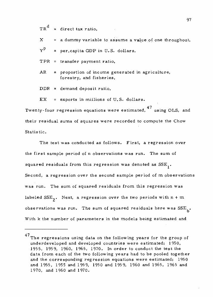
97
TR = direct tax ratio,
X = a dummy variable to assume a value of one throughout,
Y = per^capita GDP in U.S. dollars,
TPR = transfer payment ratio,
AR = proportion of income generated in agriculture, forestry, and fisheries,
DDR = demand deposit ratio,
EX = exports in millions of U.S, dollars.
47 Twenty-four regression equations were estimated, using OLS, and
their residual sums of squares were recorded to compute the Chow
Statistic.
The test was conducted as follows. First, a regression over
the first sample period of n observations was run. The sum of
squared residuals from this regression was denoted as SSE .
Second, a regression over the second sample period of m observations
was run. The sum of squared residuals from this regression was
labeled SSE . Next, a regression over the two periods with n + m
observations was run. The sum of squared residuals here was SSE, . b
With k the number of parameters in the models being estimated and
47 The regressions using data on the following years for the group of underdeveloped and developed countries were estimated: 1950, 1955, 1959, I960, 1965, 1970. In order to conduct the test the data from each of the two following years had to be pooled together and the corresponding regression equations were estimated: 1950 and 1955, 1955 and 1959, 1950 and 195 9, I960 and 1965, 1965 and 1970, and I960 and 1970.

98
b = n + m then the quantity
(SSE^ - (SSE + SSEn/k P _ b 1 ^
(SSE + SSE2)/b - 2k
is distributed as an F statistic with k and b - 2k degrees of freedom.
Tables 17 and 18 give the results for the group of underdeveloped and
developed countries, rexpectively.
Interpreting the Results
The extremely low F values from Tables 17 and 18 indicate
that there was no tax structural change during the periods involved.
It was concluded that in the short-run and long-run the hypothe-
sis of an unchanging tax structure could not be rejected.
The results showed that no significant change in TR has been
observed. The rate of change in TR has been the same over the
periods involved. It was observed in the last section that TR for
both of these groups has been decreasing. The results in this section
confirmed those of the last section and showed that the decrease in
TR has been taking place at a constant rate. Thus, a linear multiple
regression is a suitable one for analyzing TR .
Conclusions and Generalization
1. The hypothesis of structural tax changes was rejected for
both the group of underdeveloped and developed countries.
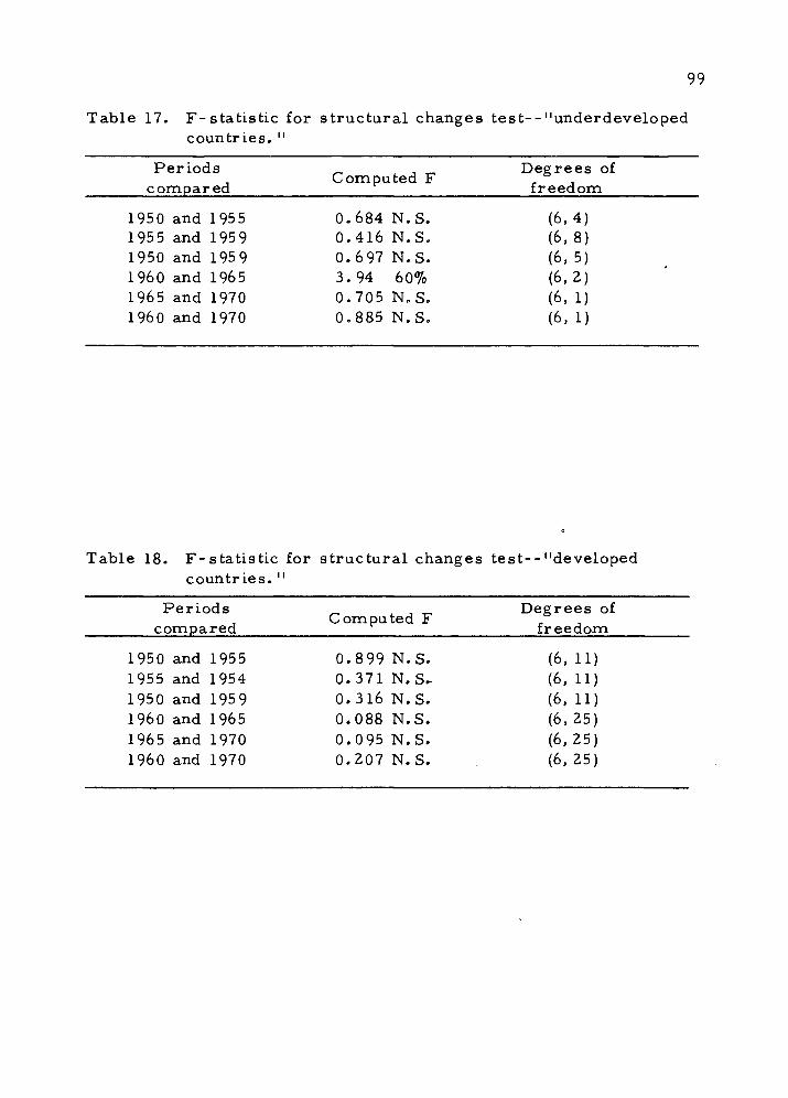
99
Table 17. F-statistic for structural changes test--"underdeveloped countries. "
Periods compared
Computed F Degrees of freedom
1950 and 1955 0.684 N.S. (6,4) 1955 and 1959 0.416 N.S. (6,8) 1950 and 195 9 0.697 N.S. (6,5) I960 and 1965 3.94 60% (6,2) 1965 and 1970 0.705 N.S. (6, 1) I960 and 1970 0.885 N.S. (6, 1)
Table 18. F-statistic for structural changes test--"developed countries. "
Periods compared
Computed F Degrees of
freedom
1950 and 1955 0.899 N.S. (6, 11) 1955 and 1954 0.371 N.S. (6, 11) 1950 and 1959 0.316 N.S. (6, 11) I960 and 1965 0.088 N.S. (6,25) 1965 and 1970 0.095 N.S. (6,25) I960 and 1970 0.207 N.S. (6,25)

100
2. TR experienced a constant rate of decrease for these
groups of countries.
Indirect and International Trade Taxes
Social and cultural backgrounds of a country play a relatively
important role in its tax policy. Lack of understanding among the
public, in underdeveloped countries, as to what the objectives of
taxation are, plus administrative and political obstacles, have put
pressure on the governments of these countries to collect taxes whose
direct impact on the public is minimized, or at least disguised.
It was hypothesized that for the group of underdeveloped coun-
tries in the first decade, the bulk of the tax revenue was collected
from indirect sources including international trade taxes. The same
hypothesis was formed for the group of underdeveloped countries in
the second decade.
The procedure used to test such hypotheses was that of compar-
ing means of the indirect and trade tax ratios (TR ) of underdeveloped
countries for each decade. The null and alternative hypotheses are
formulated as follows.
iti H : The mean of the indirect and trade taxes ratio (TR ) for
o
the group of underdeveloped countries is equal to the
grand mean of TR for all the countries, excluding the
group of underdeveloped countries, for each decade.

101
H : The mean of the indirect and trade taxes ratio (TR1*-1) for a
the group of underdeveloped countries is greater than the
grand mean of TR for all the countries, excluding the
group of underdeveloped countries, for each decade.
The test was conducted as follows. First, the mean of TR for the
group of underdeveloped countries in each decade was calculated
(X ), where f refers to the first decade and u to the group of under-
developed countries. Second, the grand mean of TR for the group
of developing and developed countries was calculated and denoted by
X , where d refers to the group of developing and developed coun-
tries. Steps one and two were followed for the second decade provid-
ing us with mean of TR denoted by X , and X ,, where s denotes su sd
the second decade. Letting S be the standard error, then
pi N
(nfu-1)Sfu+(nfd-1)Sfd
fu fd
and
pa \|
(n - 1)S2 + (n - 1)S2
su su sd sd n + n - 2
su sd
where p is the pooled standard deviation. S, , S,,, S , and S , fu fd su sd
were estimated. The
t, = X
fu " Xfd t
^
1 1 nfu "fd

102
X " X A su sd
ps n n su sd
are distributed as t statistic with n + n, - 2, and n + n - 2 fu fd su sd
degrees of freedom, respectively.
The null and alternative hypotheses were reformulated as
follows.
H : Xr = X., or Xr - xV = 0
o fu fd fu fd
H : X. > X., a fu fd
and
H:X =XnorX - X , o su sd su sd
H : X > X . a su sd
U sing equations for t and t we found I. s
.69540 - .53304
. 161
= 9.66, 1 1
149 + 240
and
.66069 - .56414 = 5.518
. 168 i i i
+ 116 451
Since the critical value of t at 1 percent level is 2.326 we see that the
alternative hypothesis should be maintained.

103
It was felt that the extensive reliance of underdeveloped coun-
tries on international trade taxes might have been responsible for the
significant difference between the two means. Consequently, a test
of difference between means was performed. This time the means
of the international trade taxes were compared and other indirect
taxes were excluded. The same procedure, as described above, was
used to test the null hypothesis that the mean of the trade tax ratio
it (TR ) of the group of underdeveloped countries is equal to the grand
mean of TR for all the countries, excluding the group of under-
developed countries, for each decade. The computed t values for
testing this hypothesis for the first and second decade, respectively,
follow.
.41836 - .17853 t = mzzz^zzzin = i ^. o J , f
.182 1 1 149 + 240
and
t = ♦32618--2339 = 5.00 s
.177 Mr ♦ ' 116 451
Since the critical value of t at the 1 percent level is 2. 326 we see that
.the null hypotheses should not be accepted. That is, the mean of the
international trade tax ratios for the group of underdeveloped coun-
it tries is significantly greater than the grand means of TR for all the
countries, excluding the group of underdeveloped countries, for each
decade.
104
Conclusion and Generalization
It is maintained that the mean of the indirect and trade Jax ratio
fQJL~t)^e«g^o,u,p^o^und,erde,velQped countxie.s,=ksKj:_3ign.ificantly, gxjeajtgr. tjasuv.
the gran^jneanjo^btained by using the data from the group of developing
and developed^countrijss.
Trade taxes constituted most of the total indirect and trade
taxes collected by this group of countries and is primarily responsible
for the significant difference between the two means.
Relatively speaking, the group of underdeveloped countries has
relied more heavily on indirect and trade taxes for their tax revenue
purposes than the developed and developing countries. The same was
true when trade taxes were examined separately.
International Trade Taxes
As one of the components of total tax revenue, trade taxes have
played an important role in the revenue structure of LDCs. Despite
the importance that is assigned to trade taxes, it was hypothesized
that the relative importance of trade taxes in total tax revenue
(TRl ) peaked during the first decade and declined in the second
decade, as the countries developed, and that-the majority of countries
have been forced to cut back or at least stop' increasing their relative
reliance on such taxes.

105
A model of the following nature was postulated.
TRit = ^.i^V^z^V^it^ + V^it,^
b5(ARit(5)+b6(DDRit)6
)
where
i = 1, 2, . . . , N (number of countries, depending upon the group or groups of the countries in the model),
t = 1, 2, . . . , T (number of years, depending on the decade being analyzed),
it TR = international trade tax ratio,
X = a dummy variable to assume a value of one throughout,
p Y = per capita GDP in U.S. dollars,
OP = openness,
TPR = transfer payment ratio,
AR = proportion of income generated in agriculture, forestry, and fisheries,
DDR = demand deposit ratio.
OLS was used to estimate the parameters in the above multiple
regression model. The Durbin-Watson Statistic was calculated for
the models. It was not possible to reject the hypothesis that auto-
regression disturbances were present. The Durbin approach was
used to correct for autoregression.
Due to its special relation to TR , it was assumed that OP
would carry a positive sign whether the relative reliance on TR is
increqsing or decreasing.

106
Table 19a presents the models corrected for autoregression
along with their necessary statistics. Best models are recorded in
Table 19b.
Interpreting the Results
The regression results obtained from analyzing 41 countries,
for 1950-1959 period, explained some of the variations in TR .
The F value is significant at about the 60 percent level of confidence.
None of the variables except TPR, which is significant at the 95 per-
cent confidence level, are significant. After the best model was
selected it was not possible to reject the hypothesis that the relative
reliance on trade taxes increased during the first decade. Both of the
variables in the model carried a positive sign. TPR was significant
at the 95 percent level of confidence and DDR was significant at the
2 50 percent level. The F value and the R are significant at the 90
percent level of confidence for the best model.
Analysis of the data from the second decade for all 46 countries
did support the hypothesis that trade taxes have been losing their
relative importance as a total tax revenue as their economies
48 The following countries were excluded from this analysis due to the lack of data on one or more variables: El Salvador, Iraq, Lebanon, Philippines, Thailand, Turkey, Sweden, Switzerland, Jordan, and Denmark.

107
developed. The F value for the model is highly significant at
49 P the 99 percent level of confidence. Y carried a negative sign and was
significant at the 95 percent level of confidence. OP carried a posi-
tive sign (as assumed) and was highly significant. The significance of
OP for the second decade showed that trade taxes responded more
systematically to the changes in the volume of exports and imports
in the second decade as compared to the first decade. The sign for
TPR is positive but not significant, where DDR carried a negative
sign and was significant at the 50 percent level of confidence.
Based on the results obtained from analyzing the data from the
first and the second decade, it was concluded that for all the sample
countries taken together, TR increased during the first decade and
decreased during the second decade. One may suspect that interna-
tional and interregional trade agreements, which have gained in rela-
tive strength in recent years, have been somewhat effective.
The data on the group of developing and underdeveloped coun-
tries (called LDCs), during the first decade, were also examined.
The result was equally satisfactory. YP, OP, TPR and DDR
carried positive signs to support the hypothesis of increasing relative
49 Iraq, Egypt, Lebanon, Turkey, Jordan, Denmark, and Switzerland are excluded from this analysis.
50 El Salvador, Iraq, Lebanon, Philippines, Thailand, Turkey, and Jordan were excluded from this analysis.

108
Table 19. Summary table of regression analysis for international trade tax ratio.
** 2 The coefficients, or F values or R , are significant at the 99 percent confidence level.
* 2 The coefficients, or F values or R , are significant at the 97.5 percent confidence level.
o 2 The coefficients, or F values or R , are significant at the 95 percent confidence level.
+ 2 The coefficients, or F values or R , are significant at the 90 percent confidence level.
x 2 The coefficients, or F values or R , are significant at the 80 percent confidence level.
(S 2 The coefficients, or F values or R , are significant at the 60 percent confidence level.
b Reject the hypothesis that autoregression is present at the 99 percent confidence level.
Figures in parentheses are the standard error of the regression coefficients.

Table 19. Summary table of regression analysis for international trade tax ratio. (TR ).
Groups and years a. The model (corrected for autoregression)
Constant Y* OP TPR AR DDR R
Durbin- Watson
St.
First decade, developing and underdeveloped groups (LDCs) .0139 .000098 .0747 .142+ .0108 .0482
(.00908) (.000080) (.0908) (.088) (.1606) (.142) ,033^ l.OS® U7ll
Second decade, developing and underdeveloped groups (LDCs)
First decade, all countries
Second decade, all countries
.0084 -.0000356 .204** .0832 -.139 -.0117 (.0041) (.000037) (.0606) (.103) (.0837) (.0658)
.0087 -.0000138 .0231 .134° .023 .0884 (.00557) (.0000361) (.0576) (.0606) (.124) (.106)
.00675 -.0000182° .201** .00981 -.0823 .0454 (.00295) (.00000901) (.0500) (.0676) (.0688) (.0506)
,056* 2.81* 1.75b
.022^ 1.13^ l.82t
. 047** 4. 44** 2.02
First decade, developing and underdeveloped groups (LDCs)
b. The best model
.0173 .000084 (.00533) (.0000747)
. US'1' (.0866)
.028+ 2.27+ 1.69b
Second decade, developing and underdeveloped groups (LDCs)
First decade, all countries
.00698 (.00296)
.0088 (.00467)
** .208
(.0658) -.123 (.0823)
.135° (.0601)
.0757 (. 104)
. 050 6. 25 1. 74
.020+ 2.6S+ 1.81b
Second decade, all countries .0053 -.0000191 .198 (.00231) (.00000889) (.0499)
-.077 (.0684)
.045 7.14 2.01
o

110
reliance on trade taxes for the group of LDCs during the first decade.
Out of five independent variables in the model only TPR was signifi-
cant at the 90 percent level of confidence. Y , and OP were signifi-
cant at the 70 and 60 percent level of confidence, respectively. AR
with a positive sign (contrary to the hypothesis) was not significant.
The best model included YP and TPR. YP was significant at the 70
percent level of confidence, and TPR was significant at the 90 percent
level.
The results obtained from analyzing the data for the second
decade for the group of LDCs did not provide evidence that this group
51 has been decreasing their relative reliance on trade taxes. This
supports the assertion made earlier with respect to LDCs, especially
underdeveloped countries, and their heavy reliance on trade taxes. It
is believed that the presence of underdeveloped countries in this
analysis is mostly responsible for such results, as the group of
developing countries exercised a high degree of reliance on direct
taxes during the second decade which necessitated less dependence on
trade taxes. A negative sign associated with Y supported this belief
to some extent. Y is significant at the 60 percent level of confidence.
However, the best model includes OP and AR significant at the
99 and 80 percent level of confidence respectively. It is concluded
51 Egypt, Iraq, Lebanon, Turkey, and Jordan were excluded.

Ill
that for the group of LDCs, especially underdeveloped countries, trade
taxes still play an important role in the budget of their governments.
Conclusions and Generalization
The following conclusions and generalization are based upon the
results obtained for this section.
1. The general hypotheses of increasing TR during the first
decade and decreasing TR during the second decade for all the
countries were maintained. Pooling these two statements provided a
strong base for accepting the posed hypothesis that reliance on inter-
national trade taxes has peaked. The results also showed that the
majority of countries have been forced to cut back or, at least, to
stop increasing their reliance on such taxes.
2. A more systematic approach has been followed in terms of
collecting trade taxes. It is possible to assume that during recejit
years, most of the countries changed their trade tax policies accord-
ing to the variations in the general volume of trade.
3. It was concluded that the trade agreements, which have
increased in numbers and importance in recent years, have effectively
decreased the relative importance of trade taxes in total tax revenue
of the governments in the recent years.
4. It was not possible to accept the hypothesis of decreasing
TR during the second decade for the group of LDCs. However, this

112
was felt to be due to the presence of underdeveloped countries,
which still relied heavily upon trade taxes.
The Case of Highly Developed Countries
Direct taxes, especially the individual income tax and the
corporate profit tax, for years have been proposed as the most
equitable and efficient type of tax. Advocates of this type of tax have
been defending it on the basis of its built-in flexibility. It seems
justified to test the tax structure of those countries--mainly highly
developed countries--that try to employ the "most efficient" type of
taxes. The objective was to clarify direction of the effect that the
"high degree of economic development" has had on tax systems of
highly developed countries. The following explicit hypothesis was
formed. The more advanced countries within the group of highly
developed countries, such as those in Western Europe and North
America, due to their high degree of economic development, have
increased their relative reliance on sophisticated techniques of tax;
collection and thus, increased their indirect tax ratio during the
recent years, as their economies have developed. •
The following relationship was postulated to test this hypothesis.
TR' = b.OC.. J + b.fY?. ,) +b,(OF.. ,) - b.(AR.. .) it 1 it, 1 2 it,2 3 it, 3 4 it, 4
- b_(DDR ) +b,(TSDR,f ) (1) 5 it, 5 6 it, 6

113
where
i = 1, 2, . . . , 12 (number of countries),
t = 1, 2, . . . , 13 (number of years),
TR = indirect tax ratio (excluding trade taxes),
Y^ = per capita GDP in U.S. dollars,
OP = openness,
AR = Proportion of income generated in agriculture, forestry, and fisheries,
DDR = demand deposit ratio,
TSDR = time and savings deposit ratio.
First, the data for the 10 countries of Western Europe for the
/ 52 1960-1972 period were exanained. The result of a multiple
53 regression analysis using OL.S follows.
TR1* = .0242 + .0000206(YP)X + . 159(OP)X - .621(AR)X
(.0067) (.0000127) (.118) (.460)
- .228(DDR)0 + . 100(TSDR) , (1. a) (.114) (.105)
with R2 = .078X, F = 1.71X and D-W St. = 1.98b .
Note; Figures in the parentheses are standard errors of regression coefficients. **
52 The countries included in the analysis were Austria, Denmark, Finland, France, Italy, Netherlands, Norway, Sweden, Switzerland, and the U. K.
53 The equation presented is the one corrected for autoregression using the Durbin approach.
54 Where o, +, and x indicate that the coefficients, or F values or R^, are significant at 95, 90, and 80 percent confidence level

114
All of the variables in the model carried the expected sign to strongly
support the hypothesis. The best model selected includes the follow-
ing variables.
TR1* = .0263 + .0000196(YP)X + . l68(OP)X - .610(AR)X
(.0063) (.0000126) (.118) (.460)
- .222(DDR)+ (l.a. i) (.114)
with R2 = .07X) F = 1. 91X, and D-W St. = 1.98
Note: Figures in parentheses are standard errors of regression coefficients.
Second, the U.S. and Canada were added to the analysis. The follow-
ing is the equation obtained after analyzing the data.
TR1* = .063 + .00000424(YP) + . 197(OP)+ - . 521(AR)X
(.0064) (.0000113) (.112) (.432)
- .242(DDR)0 + .0281(TSDR) (l.b) (.109) (.094)
with R = .059X, F=1.56X, and D-W St. = 1.70 .
The best model was selected and reported here for those countries.
TRL* = .028 + . 189(OP)+ - „523(AR)X - .239(DDR)0 (l.b. i) (.0047) (.109) (.429) (.108)
Oil 1-
with R =.057, F = 2.56 and D-W St. = 1.70 .
An F test was conducted to test the hypothesis as to whether the
addition of the U.S. and Canada to the sample data resulted in a
significant change in our model.
respectively, b indicates that autoregression is absent with 99 per- cent level of confidence.
115
For the sample countries and the period under consideration
here an F of 1.65 represents a 95 percent confidence level. The
calculated F value was 1. 10. Since the critical value of F (24, 101) is
higher than the calculated F value we conclude that addition of U.S.
and Canada to the sample did not effect the regression coefficients of
55 1. a significantly, i.e., the coefficients of the whole model l.a and
1. b are not significantly different.
Interpreting the Results
The regression results obtained from analyzing the data for
10 highly developed countries, for the period 1960-1972, support our
hypothesis of a rising relative importance of indirect taxes as highly
developed countries developed yet further. All the variables carry
the expected signs. Y , OP and AR are significant at the 80 percent
level of confidence. DDR, along with its expected negative sign for
highly developed countries, is significant at the 95 percent level of
confidence. TSDR was only significant at the 60 percent level of
confidence, and consequently it was dropped out of the model although
it carried the hypothesized sign.
Based on 1. a, and its best model 1. a. i, it was concluded that
the highly developed countries of Western Europe have been
55 The test employed was the familiar Chow test (see footnote 35,
P- 73).
116
increasing their relative reliance on indirect tax sources. The sharp
increase in reliance on this type of tax held when tax ratio for the
group of developed countries during the second decade was analyzed.
It can also be concluded that the relatively high reliance on indirect
taxes (not direct taxes) during the second decade is responsible for
the direct relationship that was found between total tax ratio (TR) and
degree of economic development for the group of developed countries.
Inclusion of U.S. and Canada in the sample did not significantly
change the regression coefficients of l.a. Equation l.b thus supported
the hypothesis.
The increase in indirect tax ratio, as a component of total tax,
presented a valid explanation to the results obtained from analyzing
direct and total tax ratios for the group of developed countries. When
TR showed an increase during the second decade, the question was
raised as to whether the countries that shifted from the second group
in the first decade to the third group during the second decade were
responsible. The situation became even less clear when it was
observed that the direct tax ratio had been decreasing for the group
of developed countries during the second decade. It was concluded,
however, that the effect of shifted countries on the results for TR was
56 statistically insignificant.
_
It is interesting to note that out of the 12 countries in the analysis of this section, 10 were the ones that fell in the third group during the first decade. The third group in the first decade included 14

117
The analysis of this section provided an answer to these contra-
dictions. Comparison of the best models, l.b, and the model for
direct tax ratio for the group of developed countries during the same
period, was interesting. Both of the models present OP and DDR as
their variables, but the signs for these variables are opposite.
The possibility of using more sophosticated techniques for
indirect tax collection in the developed countries decreased their
relative reliance on direct taxes, but simultaneously increased their
tax revenue as a percentage of GDP. Thus direct and indirect tax
ratios have moved in opposite directions for the group of highly
developed countries during the second decade. This is an important
finding in terms of changes in the tax components.
There are two reasons for this distinct shift in the tax com-
ponents in highly developed countries. (1) As is implicit in the
hypothesis, these countries possess the techniques, administrative
capacity, and experience to employ indirect taxes such as turnover
and value added taxes. (2) As it was observed, the public sector in
these countries has been growing rapidly increasing their govern-
ments' revenue needs. Since the direct tax rates were already high,
countries. It follows that this analysis is almost identical to ana- lyzing the group of countries which were grouped as "developed" during the first decade and remained in that group during the second decade, although they may have experienced a high rate of economic growth.

118
the best alternative was indirect taxes. Public pressure on politicians
and the high degree of competition involved in politics of these
countries, forced the policy makers (not economists) to increase their
tax revenue through "hidden sources" of indirect taxes where the
57 direct impact is not strongly felt or easily identified by individuals.
Conclusions and Generalization
1. The hypothesis that highly developed countries, due to their
high degree of economic development, have been able to increase their
relative reliance on sophisticated techniques of indirect tax collection
as their economy developed, was maintained.
2. It was concluded that the developed countries decreased
their relative reliance on direct taxes during the second decade due
to the possibility of increasing their indirect tax; revenues.
3. A distinct shift in the tax components of developed countries
from direct to indirect tax was observed.
4. The relative reliance on indirect taxes was sufficient to
result in an upward increase in total taxes as a percentage of GDP.
57 It is not intended to conclude that the fiscal impact of direct and indirect taxes on the individuals is distinctively different. Depend- ing on the types of direct or indirect taxes, similar as well as dissimilar final impacts might result.
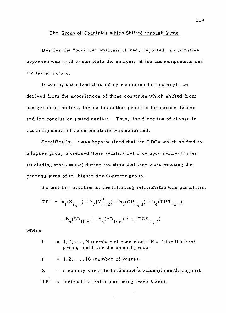
119
The Group of Countries which Shifted through Time
Besides the "positive" analysis already reported, a normative
approach was used to complete the analysis of the tax components and
the tax structure.
It was hypothesized that policy recommendations might be
derived from the experiences of those countries which shifted from
one group in the first decade to another group in the second decade
and the conclusion stated earlier. Thus, the direction of change in
tax components of those countries was examined.
Specifically, it was hypothesized that the LDCs which shifted to
a higher group increased their relative reliance upon indirect taxes
(excluding trade taxes) during the time that they were meeting the
prerequisites of the higher development group.
To test this hypothesis, the following relationship was postulated.
TRL = b1(X.t(1)+b2(Y[)t)2)+b3(OP.ti3, + b4(TPR.t(4)
b_(ER.. ,) - b,(AR.f ) + b7(DDR., ) 5 it, 5 6 it,6 7 it, 7
where
i = 1, 2, . . . , N (number of countries), N = 7 for the first group, and 6 for the second group,
t = 1, 2, . . . , 10 (number of years),
X = a dummy variable to assume a, value ol one..throughout,
TR = indirect tax ratio (excluding trade taxes),

120
p Y = per capita GDP in U. S. dollars,
OP = openness,
TPR = transfer payment ratio,
ER = education ratio,
AR = proportion of income generated in agriculture, forestry, and fisheries,
DDR = demand deposit ratio.
An identical model was used to see whether and in what direction
direct taxes might have changed for these countries. The dependent
variable was TR .
The countries of the first group in the first decade that shifted
to the second group for the second decade were examined. The
results of the regression analysis on this group of countries are
presented in Table 20. The results shown in Table 20a are for the
models after correcting for autoregressive disturbance reflected CO
through a low value of the Durbin-Watson Statistics. The best
models selected are recorded in Table 20b.
To determine whether the tax revenue of these countries (when
trade taxes are excluded) increased, a third regression model was
run. The dependent variable used was total tax revenue, excluding
trade taxes, divided by GDP, (TR ). The independent variables are
This applies to all the models in Table 20.

Table 20. Summary table of regression analyses for the group of countries which shifted.
Group and type of dependent variable
Dependent variable
a. The model (corrected for autoregression)
Constant : YP OP TPR ER AR DDR
.00746 -.000337° .336+ -.038 -.233 1. 03** .618+
(.0132) (.000161) (. 193) (.118) (.213) (.33) (. 326)
.0641 -.000166 .0037 .099 .089 -.43+ .079 (.0305) (.000143) (. 155) (.117) (.211) (. 242) (. 260)
.0161 .0000625* .0213 .00316 .0138 -.127** -.0337 (.00557) (.0000243) (.0261) (.0203) (.0364) (.0395) (. 0432)
.291 .0000251 -.301 .0983 -1.39* .246 (. 194) (.000152) (. 329) (.26) (.597) (.513)
.0581 -.00011° -. 245** -.0311 .254 -.056 (.014) (. 0000502) (.079) (.077) (.231) .(. 157)
.071 .000058** .0549 .0137 -. 23** .0312 (.0401) (. 0000189) (.0503) (.030) (. 0664) (.0579)
b. The best model
.0075 -. 000349° -. 349+ -.23 1.006** .621+
(.013) (. 000154) (.186) (.210) (.318) (.321)
.076 -.000119 -.466*
(.012) (.000103) (. 182)
.0146 .000051** -.116** (.0023) (.0000177) (.030)
F value
D^urbin- Watson
St.
First group with indirect tax TR ratio as dependent variable
d First group with direct tax TR ratio as dependent variable
First group with total tax ratio TR (excluding trade taxes) as dependent variable
Second group with indirect tax TR ratio as dependent variable
d Second group with direct tax TR ratio as dependent variable
Second group with total tax TR~ ratio (excluding trade taxes) as dependent variable
First group with indirect tax TR ratio as dependent variable
d First group with direct tax TR ratio as dependent variable
di
-di
First group with total tax ratio TR (excluding trade taxes) as dependent variable
di
,373* 3. 17* 2. 25
.199 1.33 1.58
. 445** 4.27** 1.71
,212° 2.43° 2.05b
o o b ,230 2.67 1.57
,663** 17.73** 2.24
, 370** 3.88** 2.18
, 174° 3.80° 1. 64b
,421** 13.1** 1.84
(Continuedion next page)
N>

Table 20. (Continued)
Group and type of Dependent The best model (continued)
R2
value
Durbin-
Watson St,
dependent variable variable Constant YP OP TPR ER AR DDR
Second group with indirect tax TR ratio as dependent variable
c Second group with direct tax TR ratio as dependent variable
Second group with total tax ratio (excluding trade taxes) TR as dependent variable
di
.366 (. 0576)
** .0528 -.00011 -.238
(.00761) (.000049) (.076)
.094 ,000056 .057 (.0128) (.0000173) (.0468)
-1.62 (.484)
.251 (. 226)
** -.256 (.0563)
.186 11.2 2.18
. 225 4.56 1. 60
. 659** 30. 28** 2. 32b
** 2 The coefficients, or F values or R , are significant at the 99 percent confidence level.
* 2 The coefficients, or F values or R , are significant at the 97.5 percent confidence level.
o 2 The coefficients, or F values or R , are significant at the 95 percent confidence level.
+ 2 The coefficients, or F values or R , are significant at the 90 percent confidence level.
x 2 The coefficients, or F values or R , are significant at the 80 percent confidence level.
b Reject the hypothesis that autoregression is present at the 99 percent confidence level.
c The Durbin-Watson Statistic is inconclusive.
Figures in parentheses are the standard errors of the regression coefficients.

123
the same as those in the above equation. The results obtained for
this model together with its best model are reported in Table ZO.
When the countries of the second group in the first decade that
shifted to the third group in the second decade were analyzed, a
relatively high degree of multicolinearity was observed between AR
and ER. ER was then dropped from the models for this group, as
reported in Table ZO.
The examination of the tax structure of LDCs which shifted
proceeded towards the comparison of their indirect tax ratios with
the indirect'tax ratios of those LDCs which did not shift. It was
hypothesized that the group of underdeveloped countries which shifted
to the group of developing countries relied relatively more heavily on
indirect taxes than those underdeveloped countries which did not shift.
Further it was hypothesized that the group of developing countries,
which shifted to the group of developed countries, relied relatively
more heavily on indirect taxes than those developing countries which
did not shift.
The procedure used to test such hypotheses was that of compar-
ing means of the indirect tax ratios (TR ) of those countries which
shifted with that of the countries which did not. The test was con-
ducted as follows. First, the mean of TR for the group of under-
developed countries which shifted was calculated (X ), where s su
refers to the countries which shifted and u to the group of

124
underdeveloped countries. Second, the mean of TR for the group of
underdeveloped countries which did not shift was calculated and
denoted by X . Steps one and two were followed for the group of u
developing countries providing us with means of TR for the group of
developing countries which shifted and the developing countries which
did not. These means were denoted by X and X respectively, sd d
where d refers to the group of developing countries. Letting S be the
standard error, then
pu \
(n -1)S2 + (n -1)S2
su su u n + n - 2
su u
and
pd
i '"sd" "4 + 'V "Sd
n , + n , - 2 sd d
where p is the pooled standard deviation. S ,5,3,, and S, su u sd d
were estimated. The
u
X - X su u
pu 1 1 + — . n n
^ su u
sd d
pd 1 _1_
n A nA sd d
are distributed as t statistics with n + n - 2, and n , + n, - 2 su u sd d

125
degrees of freedom, respectively. The null and alternative hypotheses
were reformulated as follows.
H: X =XorX - X = 0 o su u su u
H : X > X , a su u
H : X , = X,, or X , - X, = 0 o sd d sd d
H : X > XJ , a sd d
using the equation for t and t we found u d
.3088 - .22449
. 102
= 4.70, i_ _L
\|6l + 69
and
.47075 - .35434 = 3.88
. 150 1_ _1_ \| 50 + 50-
since the critical value of 1(99,98) is 2. 38 and t(99, 128) is 2. 35 we
see that both of the above alternative hypotheses should be main-
tained.
Interpreting the Results
The analysis of the indirect tax. ratio for the group of under-
developed countries which shifted to the group of developing countries
did not seem to provide strong evidence as to what direction those
taxes were moving.

126
The direct tax ratio was analyzed to see whether the degree of
relative reliance on those taxes had changed. Y , which theoreti-
cally should be positively related to TR , carried a negative sign and
was significant at only the 70 percent level of confidence. This would
indicate that direct taxes, as a component of total tax revenue, had
decreased. AR was the only other significant variable at the 80 per-
cent level of confidence. ER carried a positive sign (contrary to our
assumption) and was not significant. Since the total model was not
significant, it was not possible to draw any conclusions.
If neither TR nor TR were increasing, then a decrease in
total tax ratio (excluding trade taxes) should have been observed.
In order to extract any effect that heavy reliance on trade taxes
might have had on the total tax ratio, it was redefined as total direct
taxes plus total indirect taxes (excluding trade taxes) divided by GDP
Hi Hi and was denoted by TR . As recorded in Table 20 TR increased
as these countries developed. Y , along with its positive sign, was
significant at the 97.5 percent level of confidence. OP, TPR, and
DDR carried the expected signs but were not significant. AR carried
a negative sign, as expected, and was significant at the 99 percent
level of confidence. The F value for the model was significant at the
99 percent level of confidence.
Examination of the model for TR led us to conclude that the
total tax ratio, with trade taxes excluded, had increased with economic

127
growth in these countries. It was then concluded that these countries
relied on other types of taxes rather than just trade taxes.
If the total tax ratio excluding trade taxes has been increasing,
and if the direct tax ratio has not been increasing--if not decreasing--
then it followed that the increase in indirect tax ratio is responsible
for the increase in total tax ratio of the group of underdeveloped
59 countries which shifted to the group of developing countries.
This assertion was maintained after a careful examination of the
model for indirect tax ratio. The negative sign, carried by Y ,
reflected the fact that the higher per capita GDP for the under-
developed countries, the more direct taxes were collected in these
countries at their low stage of economic development. This is the
same as saying that the higher per capita GDP, the less indirect
taxes need to be collected, given other things equal.
Being an underdeveloped country, a country will rely heavily on
trade taxes. However, the international trade sector in these coun-
tries is not stable, and fluctuates with the changes in the world mar-
60 ket, as does the tax revenue collected through those sources. A
59 This was not true in the case of all the underdeveloped countries in the first decade. Not only did TR^ decrease for these countries, but the increase in trade taxes as the only element in their total tax revenue resulted in an increase in the total tax ratio (see Tables 14 and 16).
This is one of the reasons that trade taxes are not a promising source of tax revenue for those countries.

128
decrease in the volume of exports and/or imports results in a rela-
tively significant loss of tax revenue associated with trade taxes. The
best substitute for trade taxes, at that level of development, has been
indirect taxes to provide the necessary funds to be used for develop-
ment purposes by the government. It follows that antegative sign
should be expected for OP in relation to TR in these countries.
Being at the stage of trying to initiate development programs,
the agricultural sector received special attention. These countries
concentrated on development of the agricultural sector during their
early transition period and developed this sector along with other
sectors of the economy. The positive sign for AR reflects the
sharp increase in indirect taxes rates levied on agricultural products,
which were the dominant economic sector in most of these countries.
DDR carried a positive sign, as was expected, and was significant
at the 80 percent level of confidence. ER also carried the expected
sign and was significant at the 70 percent level of confidence. TPR
with its negative sign was dropped out, when the best model was
selected.
The proportion of income generated in agriculture will continue to decline as other sectors of the economy develop. It is the absolute value of the income generated in this sector that enables the govern- ment of these countries to increase their indirect tax revenue by imposing a tax on agricultural products. Experience shows that ,, most of the underdeveloped economies are agricultural oriented rather than industrial.
129
It was concluded that the sharp increase in TR , i.e., the
relative reliance on indirect taxes in total tax. revenue, explained most
of the increase in the total tax ratio for the group of underdeveloped
countries which shifted to the group of developing countries. Those
countries were the only group of countries which explored and used
other sources of tatxation other than just trade taxes. Consequently,
the governments of these countries ended up with a relatively higher
tax revenue than those countries which relied only on trade taxes.
The results obtained from analyzing the data on the group of
developing countries which shifted to the third group strongly sup-
ported the hypothesis. Not only indirect tax ratio showed an increase
during their transition but the direct tax ratio lost its relative
importance as a component of total taxes.
A positive sign for Y was not statistically significant for the
model using TR as its dependent variable. OP carried a negative
sign and was significant at the 70 percent level of confidence, support-
ing the assertion made about underdeveloped countries with regard to
its negative sign. However, trade taxes did not play as important a
role here as they did in the case of underdeveloped countries. TPR,
and DDR carried the expected positive signs but neither was signifi-
cant. The only significant variable in the model was AR at the 97. 5
percent level of confidence and carried the expected negative sign.
This group of countries had passed their underdevelopment stage and

130
development of industrial, as well as other sectors of the economy,
resulted in the reduction of the proportion of income generated in
agriculture. The model was significant at the 95 percent level of
confidence.
When the data for these countries with the direct tax ratio as
the dependent variable were used, the results were as satisfactory as
for the indirect tax ratio model. Per capita GDP carried a negative
sign and was significant at the 95 percent level of confidence. OP
also carried a negative sign and was highly significant at the 99 per-
cent level of confidence. TPR and DDR, although not significant,
carried negative signs. AR, with its positiye sign, was significant
at the 70 percent level of confidence. It was concluded that the direct
tax ratio was decreasing for these countries. However, the model for
total tax ratio (excluding trade tcixes) strongly suggested an increased
TR . This increase was attributed to the increase in indirect tax
revenue which not only compensated for the decrease in direct tax
ratio but also increased sufficiently to result in a higher tax ratio
(excluding trade taxes) for this group of countries.
Conclusions and Generalization
1. The hypothesis of heavy reliance on indirect taxes by those
countries which shifted to a higher group was maintained.

131
2„ The tax components of underdeveloped countries which
shifted moved towards a heavier reliance on indirect taxes. They
were the only group of countries which did not solely rely on trade
taxes as the source of government tax revenue. The increase in
indirect taxes, not trade or direct taxes, resulted in the increase of
their total tax; revenue, thus increasing the proportion of total taxes
as a percentage of GDP.
3. With the direct tax ratio decreasing for the group of develop-
ing countries, and their total tax ratio increasing, it was concluded
that the sharp increase in indirect tax revenue and thus the increase
in its relative importance in total tax revenue resulted in the sharp
increase of total tax ratio as a proportion of GDP.

132
VI. CONCLUDING REMARKS
Summary
There is evidence that the governments of underdeveloped as
well as developing countries must intervene in promoting the level of
investment to develop their economies. Higher tax revenues seem
to offer a promising source of funds for governments to use in attempt-
ing to secure higher levels of national investment. In order to recom-
mend suitable tax policies designed to result in higher government
revenue to be used in financing their economic development, the exist-
ing tax systems were empirically analyzed.
Sample countries were separated into three groups using
factor analysis. Group one was labeled "underdeveloped countries, "
group two "developing countries, " and the third group "developed
countries. " The group of "less developed countries" (LDCs) included
both underdeveloped and developing countries, in our analysis.
Given previous research, several econometric models
were developed and tested to provide the necessary empirical frame-
work to be used in tax policy formulation. The main objective pf
these empirical analyses was to provide a quantitative ag£rjusal^of
changes in total tax revenue as a percentage of GDP^and changes in
tax components as the economy develops. The following hypotheses
were developed and tested:

133
1. There is a direct relationship between the degree of
economic development and total tax revenue as a percentage of GDP.
2. As the economy develops, the tax structure of the country
changes towards more intensive use of direct taxes, i.e., the relative
proportion of direct taxes in total tax revenue increases.
3. Underdeveloped countries possess a more unstable tax
structure than more developed countries.
4. For the first group in the first decade, the bulkwofvthe tax
revenue was collected through indirect taxes including taxes on
international txad.e,„ i.e., the group of underdeveloped countries in
the first decade collected taxes whose direct impact on the public was
minimized, or at least disguised. The same hypothesis was formed
for the second decade.
5. The relative importance of international trade taxes in total
tax j^evenue increased during the first decaiig-and decreased during the
second decade as their economies developed. Thus the majority of
countries have been forced to cut back or at least stop increasing
their relative reliance on such taxes.
6. Countries, such as those in Western Europe and North
America, due to their high degree of economic development, have
been able to increase their relative reliance on indirect tax collection
and thus, increased their indirect tax ratio in theL sjecqnd decade as
their economies developed.

134 Since the data were divided into two decades--the first decade,
1950-1959, and the second decade, I960- 1972-- it was possible to
observe that 13 countries moved from a given group in the first decade
to another group in the second as their degree of economic develop-
ment advanced. It was hypothesize*^ that the less developed countries
which shifted to a higher group relie4 more heavily upon indirect
taxes (excluding trade taxes), during the time they were meeting the
prerequisites of the higher development group, than those countries
which did not shift. The analysis of their tax components and tax
structure along with the results obtained from past analysis, provided
useful empirical evidence for formulating tax policy for the group of
LDCs.
Conclusions
An examination of total tax revenue as a percentage of gross
domestic product through a multiple regression analysis with total
tax ratio as the dependent variable and factors reflecting the degree
of economic development as independent variables, provided evidence
for maintaining the general theory of a direct relationship between the
degree of economic development and the total tax ratio.
The group of underdeveloped countries relied heavily upon
trade taxes as a source of government revenue. The group of develop-
ing countries were able to rely on direct and indirect sources of taxa-
tion other than trade taxes.

135
Although the general hypothesis of direct relationship between
the degree of economic development and total tax ratio was maintained
in the case of developed countries, it could not be concluded that
factors indicating the degree of economic development can fully
explain the total tax ratio changes for this group during the 1950-1959
period. It was concluded that, besides the degree of economic
development, other factors, such as politics and the role of fiscal
policy in stabilization practices, have also affected variations in total
tax ratio for this group of countries.
Although a wide range of exceptions were observed, the analysis
of tax components in terms of the percentage of direct taxes in total
tax revenue, did support the general hypothesis of a direct relationship
between the degree of economic development and the increase in
relative importance of direct taxes in total tax revenue.
As for the group of underdeveloped countries, a decrease in the
direct tax ratio was observed and it was concluded that the imposition
and collection of direct taxes are practically impossible, and may
encounter numerous administrative as well as political and social
obstacles.
It became evident that direct tax collection (the increase in its
relative importance compared to other types of taxes) becomes pos-
sible when the country is at its "developing" stage. However, direct
136
taxes have been losing their relative importance in the budget of the
governments in developed countries.
A general increase in the international trade tax ratio during the
first decade and a decrease of the relative importance of trade taxes
in total tax revenue during the second decade was observed. It was
concluded that the decreasing proportion, of trade taxes/in total
revenue may have been a reflection of the effectiveness of• recSnt
trade agreements.
It was observed that, one of the most significant differences
between the tax revenue structures of developed and underdeveloped
countries was the virtually complete absence of trade taxes in the
former and their frequency and importance in the latter. In under-
developed countries, trade taxes have been easy to collect. The bor-
der has provided a convenient control point for exported and/or
imported goods. Thus, a heavy dependence on trade taxes has
developed because of the ease of levying and administering such
taxes.
The relatively high degree of economic development that pre-
vails in the countries of Western Europe and North America has
enabled them to employ sophisticated techniques of indirect tax
collection and thus increased the relative importance of indirect
taxes in their budgets during recent years.

137
It was maintained thajt.those^countries which shifted to a higher
1 group reliedjaeavily- on indirect tax sources (excluding trade taxes) j
during their preparation for the transition to a higher development
stage,-^'
Implications and Speculations
When the private sector is not active in creating enough saving
and investment for launching economic development, direct govern-
ment intervention in many economic activities is frequently recom
mended. Higher tax revenue by itself may not affect the degree of
economic development. As P.S. Heller (1974) and Please (1967)
concluded, a shift to investment rather than consumption is required
by the public sector in the LDCs to cause economic development. If
the increase in government revenue through taxation goes to consump-
tion, higher taxation may not have a meaningful effect on develop-
ment. Further, it might be well to point out that no tax should be
collected if the individuals' propensity to invest is higher than that of
the government. However, as our earlier discussion showed, this is
not the case in the LDCs, especially the underdeveloped countries
(group I).
Higher tax revenue, with increased government participation in
economic activities, may result in economic development. Still, oui
suggestions for a fiscal system (which includes a tax system) have
138
basically one common objective--that of mobilizing resources from
the private through the government sector, thereby enabling the con-
duct of economic development (see Chelliah 1969, p. 52; Due 1963,
p. 146; Hicks 1965, pp. 67-68). '
The empirical findings, discussed earlier, identified the kind of
taxes that are used when a country is underdeveloped. The group of
underdeveloped countries relied heavily upon trade taxes during both
decades. This reliance showed a decreasing trend during the second
decade when all the countries were examined, and it may be concluded
that no further relative increase in trade taxes is advisable.
The analysis of direct taxes for the combined countries of the I I
underdeveloped group showed a decrease in the direct tax ratio. This,
I along with the results obtained from analyzing the tax structure of j
those countries which were underdeveloped during the first decade
and shifted to developing in the second decade, indicated to us that
indirect taxes (excluding trade taxes), not direct taxes, played the
dominant role.
The widespread application of direct taxes has not been feasible
in underdeveloped countries and the increased application of trade
taxes may already have been relatively fully exploited.
Generally, based on the empirical findings, direct tax collection
has neither been feasible nor practical in underdeveloped countries.

139
Thus, it seems reasonable to seek alternative sources of tax. revenue
among the group of indirect taxes.
In summary, the empirical findings indicate that:
,' 1. the widespread application of direct taxes is not feasible in
underdeveloped countries,
2. the application of trade taxes in underdeveloped countries
is already largely exploited relative to other tax alternatives, and
1 3. indirect taxes offer better alternative sources of taxes than
"direct or trade taxes in these countries.
The results obtained from the statistical analysis may also be
applicable to policy recommendations regarding possibility of increas-
ing tax revenue for the group of developing countries for financing
their development.
1. The general hypothesis that the .more developed the country,
the more direct tax can be collected relative to other taxes was main-
tained, using the data for the 1960-1972 period.
2. However, there is little evidence, based on the results
obtained, that the group of developing countries made any attempt to
increase their tax revenue from dLrect sources during the first decade.
3. During the first decade, the governments of those countries
which shifted from the group of developing countries to the third group \
in the second decade concentrated their efforts on collecting and rely-
ing more heavily on indirect taxes than direct taxes.

140
4, During the second decade the developing countries did rely-
more on direct taxes as their economy developed. It was concluded
that direct tax collection, and the increase in its relative importance
compared to other types of taxes, becomes possible when the country
is at its "developing" stage.
5. However, it was concluded that continued reliance on
indirect taxes is also necessary in order to capture higher total tax
revenue, because a lag exists between the time that a country enters j
1 this stage of development and the time it actually can rely heavily
upon direct taxes.
Although it was not made explicit earlier, another conclusion
etnerges when the results obtained from analyzing indirect taxes are
examined. That is, it was observed that whenever the possibility of
direct tax collection became limited,, due to economic or other reasons,
a.jc.fXatively higher reliance..on, indLr-ect^tcLxes^was ,s.Qught.
In general, the group of developing countries have better tax
alternatives, and tax policy formulation can take on a more flexible
form than those of underdeveloped countries.
The possibility and applicability of both direct and indirect
taxes differs for countries within the developing stage. Two different
groups of developing countries should be distinguished: (1) those
countries which have just entered the developing stage and are striving
to continue their economic progress, and (2) those countries which

141
were "developing" and remained in that group, but need a higher level
of revenue to finance continued development. The more advanced
stage of economic development in the group of developing countries
as compared to underdeveloped countries, is responsible for the
possibility of direct tax collection. Most of the tax policy difficulties
identified in the case of underdeveloped countries are either absent or
have decreased in degree. This can be attributed to a more fully \
\ developed monetary economy, better communication, better education, \
i i
an increase in the number of trained personnel in public sector, and a ., /
more efficient public sector. /
In summary, based on our empirical findings, the following
speculations can be made for the group of developing countries:
1. Although direct tax collection is possible when the countries
are developing, this type of tax should be handled with care in order
to make sure that possible adverse effects on individuals' incentives
for development-oriented behavior are pninimized. This generaliza-
tion is especially important in case of income taxes when the private
sector has to play a positive role in raising the level of savings and
investment in productive activities.
2. Relatively higher reliance on indirect taxes by the group of
developing countries, which have just arrived at this stage of develop-
ment, is considered desirable due to the possible limitations that may
exist during the early periods of the developing stage in terms of

142
direct tax collection. As the economy of these countries develops,
higher reliance on direct taxes can be implemented along with the
existing indirect taxes to maximize the governments' tax revenue.
3. Although the possibility of higher direct tax collection may
result in a lower proportion of taxes collected through indirect
sources in the total tax revenue, neither those countries which were
developing nor those which enter this stage of development should be
advised to reduce their absolute level of indirect taxes.
4. In general, a pattern used by the new developed countries
can be followed by the group of developing countries. That is,
raising more and more tax revenue, through direct sources while main-
taining a high level of indirect taxes until the public pressure and
political institutions necessitates a departure from increasing the
reliance on direct taxes. At that time, these countries should be in a
position to expand and utilize new and more sophisticated types of
indirect taxation.
Suggestions for Further Research
The observation, upon reexamination of the hypotheses con-
cerning direct and indirect tax ratios, reveals that the hypotheses
may have been too broad. Limitation of data and time did not provide
the opportunity for this study to break down the components of direct
and/or indirect taxes and test for the change in these components and
143
their relationship to the degree of economic development. Neither was it
possible to examine in depth the actual tax policies followed. It
would be rewarding to examine the tax structure of those countries
which shifted, individually, to determine what their tax policy has
been.
It was established that factors other than those representing
the degree of economic development have been responsible for tax
changes especially in the case of developed countries. Identification
of those factors and their interrelation with factors representing the
degree of economic development, as well as tax changes, would be
quite useful. The type of government and the political system of a
country may, in general, affect taxation.
An important problem to be investigated is the optimum alloca-
tion of governments' higher tax revenue to achieve the highest possible
rate of economic growth and development with a reasonable degree of
stability.

144
BIBLIOGRAPHY
Adelman, Irma and Cynthia Taft Morris. 1973. Economic Growth and Social Equity in Developing Countries. Stanford: Stanford University Press.
Adelman, Irma and Cynthia Taft Morris. 1967. Society, Politics, and Economic Development: A Quantitative Approach. Baltimore: The Johns Hopkins Press.
Agarwala, A.N. and S. P. Singh (eds. ). I960. The Economics of Underdevelopment. London; Oxford University Press.
Bangs, Robert B. 1968. Financing Economic Development. Chicago: The University of Chicago Press.
Banks, F.E. 1974. "A Note on Fiscal Policy Models and Economic Development. " Public Finance XXIX (2):225-230.
Basch, Antonin. 1964. Financing Economic Development. New York: The Macmillan Company.
Baster, Nancy (ed. ). 1972. Measuring Development. London; Frank Cass & Co. Ltd.
Bauer, P. T. 1972. Dissent on Development: Studies and Debates in Development Economics. Cambridge: Harvard University Press.
Bauer, P. T. and B.S. Yamey. 1957. The Economics of Under- developed Countries. London: James Nisbet and Co. Ltd.
Baumol, W. J, 1974. "On Taxation and the Control of Externalities: Reply." American Economic Review LXIV (3):472. June.
Bhagwati, Jagdish. 1966. The Economics of Underdeveloped Countries. New York: McGraw-Hill Book Company.
Bird, Richard M. 1970a. The Growth of Government Spending in Canada. Toronto: Canadian Tax Foundation.
Bird, Richard M. 1970b. Taxation and Development. Cambridge, Massachusetts: Harvard University Press.
145
Bird, Richard M. 1973. Taxing Agricultural Land in Developing Countries. Cambridge: Harvard Law School, International Tax Program.
Bird, Richard M. and Oliver Oldman (eds. ). 1964. Readings on Taxation in Developing Countries. Baltimore: The Johns Hopkins Press.
Branson, William H. 1972. Macroeconomic Theory and Policy. New York: Harper and Row, Publishers.
Burkhead, J. and Jerry Miner. 1974. Public Expenditure. Chicago: Aldine Publishing Company.
Cadman, M. H. (ed. ). 1969. Taxation Economics. London: Macmillan and Co. Ltd.
Cairncross, A. K. 1970. "Factors in Economic Development, " in G.M. Meier, ed., Leading Issues in Economic Development. New York; Oxford University Press, pp. 504-509.
Canada Royal Commission on Taxation Report. 1966. Ottawa: Roger Duhamel, F.R.S.C. Queen's Printer and Controller of Stationary. Vol. 1-6.
Central Treaty Organization (CENTO). 1965. Symposium on Tax Administration. Tehran, Iran, March 6-12. Office of United States Economic Coordination for CENTO Affairs.
Chandavakar, A. G. 1973. "How Relevant is Finance for Develop- ment?" Finance and Development X (3):36-45. September.
Chelliah, Raja J. 1969. Fiscal Policy in Underdeveloped Countries. London; George Allen and Unwin Ltd.
Chelliah, Raja J. 1971. "Trends in Taxation in Developing Coun- tries. " International Monetary Fund Staff Papers XVIII (2):254- 331. July.
Chow, Gregory C. I960. "Test of Equality between Sets of Coeffi- cients in Two Linear Regressions. " Econometrica XXVIII (3): 591-605. July.
Committee for Economic Development. 1966. How Low Income Countries Can Advance Their Own Growth. New York: C.E.D. September.
146
Crockett, Joseph P. 1965. "Common Obstacles to Effective Tax Administration in Latin America." Joint Tax Program. Prob- lems of Tax Administration in Latin America. Baltimore; The Johns Hopkins Press, pp. 1-30.
Cutt, James. 1969. Taxation and Economic Development in India. New York: Frederick A. Praeger Publisher.
Davidson, Ralph K. 1965. "Taxation in Developing States." A paper submitted to Rehovoth Conference, Jerusalem, Israel. August.
Davidson, Ralph K. 1967. "Objectives of Tax Policy, " in David Krivine, ed. , Fiscal and Monetary Problems in Developing States. New York: Frederick A. Praeger, Publisher, pp. 229- 237.
Draper, N. R, and H. Smith. 1966. Applied Regression Analysis. New York: John Wiley and Sons, Inc.
Due, John F. 1959. Sales Taxation. Urbana; University of Illinois Press.
Due, John F. 1963. Taxation and Economic Development in Tropical Africa. Cambridge: The M.I. T. Press,
Due, John F. 1965. "Administration Criteria in the Establishment of Sales and Excise Tax Structure. " Joint Tax Program. Problems of Tax Administration in Latin America. Baltimore: The Johns Hopkins Press, pp. 413-455.
Due, John F. 1970. Indirect Tax in Developing Economies. Baltimore: The Johns Hopkins Press.
Due, John F. 1972. "Alternative Forms of Sales Taxation for a Developing Country. " Journal of Development Studies IIX (2); 263-276. January.
Enke, Stephen. 1967. "Contribution of Fiscal Policy to Develop- ment, " in David Krivine, ed. , Fiscal and Monetary Problems in Developing States. New York: Frederick A. Praeger, Pub- lisher, pp. 253-272.
Enweze, C. 1973. "Structure of Public Expenditure in Selected Developing Countries: A Time Series Study. " Manchester School of Economics and Social Studies XLI (4):430-463. December.

147
Fairbairn, Patrick. 1971. "Capital Formation and Equity in Economic Development, with Particular Reference to East Africa. " Unpublished paper. May.
Farioletti, M. 1973. "Tax Administration Funding and Fiscal Policy." National Tax Journal XXVI (1): 1-16. March.
Friedlaender, A.F., G. J. Swanson, and J. F. Due. 1973. "Estimat- ing Sales Tax Revenue Changes in Response to Changes in Personal Income and Sales Tax. Rate. " National Tax Journal XXVI (1):103-110. March.
Gandhi, Ved P. 1971. •"Wagner's Law of Public Expenditure: Do Recent Cross-Section Studies Confirm It?" Public Finance XXVI (l):44-56.
Georgakopoulos, Theodore. 1974. "The 'Excess Burden' Contro- versy in a Trading World: A Case for Special Indirect Taxes." Public Finance XXIX (2): 152-167.
Ghai, Dharam P. 1966. Taxation for Development, a Case Study of Uganda. Nairobi: East African Publishing House.
Gill, Richard T. 1967. Economic Development: Past and Present. Englewood Cliffs, New Jersey: Prentice-Hall, Inc.
Goldsmith, Raymond W. 1969- Financial Structure and Development. New Haven: Yale University Press.
Goode, Richard. 1956. The Individual Income Tax. Washington, D. C. : The Brookings Institution.
Goode, Richard. 1964. "Reconstruction of Foreign Tax Systems, " in R. Bird and O. Oldman, eds., Readings on Taxation in Developing Countries. Baltimore: The Johns Hopkins Press, pp. 169-179.
Groves, Harold M. 1959. "Income Tax Administration. " National Tax Journal XII (1):37-53. March.
Gurley, J. G. 1965. "Financial Structure in Developing Economies. " Paper submitted to Rehovoth Conference, Jerusalem. August.
Heller, P.S. 1974. "Public Investment in LDC's with Recurrent Cost Constraint: The Kenyan Case. " Quarterly Journal of Economics LXXXVIII (2):251-277. May.
148
Heller, P.S. 1975. "A Model of Public Fiscal Behavior in Develop- ing Countries: Aid, Investment, and Taxation. " American Economic Review L.XV (3):429-445. June.
Heller, W.W. 1964. "Fiscal Policy for Under-developed Countries, " in R. Bird and O. Oldman, eds., Readings on Taxation in Developing Countries. Baltimore: The Johns Hopkins Press. pp. 3-30.
Hicks, Ursula K. 1 96 1. Development from Below. Oxford: Oxford University Press.
Hicks, Ursula K. 1965. Development Finance: Planning and Control. Oxford: Clarendon Press.
Higgins, Benjamin. 1955. Financing Development of Underdeveloped Areas. Cambridge: Center for International Studies, Massa- chusetts Institute of Technology.
Higgins, Benjamin. 1968. Economic Development. London: Constable and Company Limited.
Hinrichs, Harley H. 1965. "Determinants of Government Revenue Shares among Less Developed Countries. " The Economic Journal LXXV (299):546-556. September.
Hinrichs, Harley H. 1966. A General Theory of Tax Structure Changes during Economic Development. Cambridge; The Law School of Harvard University.
International Monetary Fund. Issues 1949-1959. Balance of Payments Yearbook, Washington, D.C«
International Monetary Fund. Issues 1966, 1970, and 1974; Supple- ments to 1966/67 and 1967-68. International Financial Statistics. Washington, D.C.
Jastram, Roy W. 1940. "The Shifting of Sales Taxes. " Quarterly Journal of Economics LIV (4):673-678. August.
Jenkins, H. P.B. 1955. "Excise-Tax Shifting and Incidence; A Money Flows Approach. " Journal of Political Economy LXIII (2):125-150. April.
Johansen, Leif. 1968. Public Economics. Amsterdam: North- Holland Publishing Company.

149
Joint Tax Program. 1965. Fiscal Policy for Economic Growth in Latin America. Papers and proceedings of a conference held in Santiago, Chile, December, 1962. Baltimore: The Johns Hopkins Press.
Joint Tax Program. 1965. Problems of Tax Administration in Latin America. Baltimore: The Johns Hopkins Press.
Kaldpr, N. 1959. An Expenditure Tax. London: George Allen and Unwin Ltd.
Kaldor, N. 1963. "Will Underdeveloped Countries Lear:i to Tax." Foreign Affairs XLII (2):410-419. January.
Khan, M.Z. 1973. "The Responsiveness of Tax Yield to Increases in National Income. " Pakistan Development Review XII (4):
416-432. Winter.
Khazzoon, J. 1966. The Currency Ratio in Developing Countries. New York: Frederick A. Praeger, Publishers.
Kindle.berger, Charles P. 1965. Economic Development. New York: McGraw-Hill, Inc.
Kmenta, Jan. 1971. Elements of Econometrics. New York: The Macmillan Company.
Krause, Walter. 1961. Economic Development. San Francisco: Wadsworth Publishing Company, Inc.
Krivine, David (ed. ). 1967. Fiscal and Monetary Problems in Developing States. New York: Frederick A. Praeger, Pub- lisher.
Krishnamurty, L. 1968. "Savings and Taxation in Developing Countries: An Empirical Study. " International Bank for Reconstruction and Development, Economic Development Papers (23). August.
Lee, J. K. 1971. "Exports and the Propensity to Save in L. D. C. s. " Economic Journal XXCI (322):341-35 1. June.
Leibenstein, Harvey. I960. Economic Backwardness and Economic Growth. London: John Wiley and Sons, Inc.

150
Leuthold, Jane H. and John F. Due. 1970. "A Fiscal Policy.Model for Economic Development." Public Finance XXV (4)s5 17-533.
Leuthold, Jane H. and John F. Due. 1974. "A Fiscal Policy Model for Economic Development: A Reply. " Public Finance XXIX (2):231-235.
Lewis, W. Arthur. 1966. Development Planning. New York; Harper and Row.
Lynn, Arthur D. , Jr. (ed. ). 1969. The Property Tax and Its Administration. Madison; The University of Wisconsin Press.
Mahar, D. J. 1971. "The Growth of Public Expenditures in Selected Developing Nations: Six Caribbean Countries 1940-1965." Public Finance XXVI (l):57-74.
Mann, A. J. 1972. "The Growth of Public Expenditure in Selected Developing Nations: Six Caribbean Countries 1940-1965--A Comment. " Public Finance XXVII (3):368-369.
Marshal, J. and B. Ducros (eds. ). 1968. The Distribution of National Income. London; Macmillan.
Martin, A. andW.A. Lewis. 1956. "Patterns of Public Revenue and Expenditure. " Manchester School of Economics and Social Studies XXIV (3):203-244. September.
Meier, G. M„ andR.E. Baldwin. 1957. Economic Development. New York: John Wiley and Sons, Inc.
Meier, Gerald M. (ed. ). 1970. Leading Issues in Development Economics. New York: Oxford University Press.
Miller, Donald C. 1951. "Sales-Tax Progressivity Attributable to a Food Exemption. " National Tax Journal IV (2); 148-160. June.
Motley, B. 1973. "Sales Versus Income Taxes: A Pedagogic Note." Oxford Economic Paper XXV (2):204-212. July.
Musgrave, Richard A. and Peggy B. Musgrave. 1973. Public Finance in Theory and Practice. New York: McGraw-Hill Book Company.
151
Musgrave, R. A. 1959. The Theory of Public Finance. New York; McGraw-Hill Publishing Co.
Musgrave, R. A. 1969- Fiscal Systems. New Haven; Yale University Press.
Mynit, H. 1964. The Economics of the Developing Countries. London: Hutching son and Co. Ltd.
Mynit, H. 1971. Economic Theory and the Underdeveloped Countries. Oxford: Oxford University Press.
Neter, J. and W. Wasserman. 1974. Applied Linear Statistical Models. Homewood: Richard D. Irwin, Inc.
Nowak, Norman D. 1970. Tax Administration in Theory and Practice. New York: Praeger Publishers.
Okigbo, P.N.C. 1967. "Saving and Investment through Government Budgets, " in David Krivine, ed., Fiscal and Monetary Prob- lems in Developing States. New York: Frederick A. Praeger, Publishers, pp. 273-292.
Organization for Economic Cooperation and Development (OECD). 1968. Fiscal Policy for a Balanced Economy; Experience, Problems, and Prospects. Paris. December.
Peacock, Alan and Gerald Hauser (eds. ). 1963. Government Finance and Economic Development. OECD Publication. December.
Perera, Phillips. 1968. Development Finance: Institutions, Problems, and Prospects. New York: Frederick A. Praeger, Publishers.
Phelps, Edmund S. 1965. Fiscal Neutrality towards Economic Growth. New York: McGraw-Hill, Inc.
Please, P. 1967. "Saving through Taxation-- Reality or Mirage ?" Finance and Development IV (l):24-32. March.
Pluta, Joseph E. 1974. "Growth Patterns in U.S. Government Expenditure, 1965-1972. " National Tax Journal XXVII (1): 71-92. March.
152
Prest, A.R. 1962. Public Finance in Underdeveloped Countries. London: Weildenfeld and Nicolson.
Prest, A.R. 1973. "Public Finance; Backward Area or New Frontier?" Economica XL, (158): 12 1-135. May.
Rehovoth Conference on Fiscal and Monetary Problems in Developing States. 1965. Hebrew University, Jerusalem and Weizmann Institute of Science, Rehovoth. August 9-18. Israel.
Reuss, Frederick G. 1963. Fiscal Policy for Growth without Inflation. Baltimore: The Johns Hopkins Press.
Rostow, W.W. 1956. "The Take-off into Self-Sustained Growth. " Economic Journal LXVI (26l):25-48. March.
Sachs, Ignacy. 1964. Patterns of Public Sector in Underdeveloped Economies. New York: Asia Publishing House.
Seligman, Edwin R.A. 1969a. The Shifting and Incidence of Taxa- tion. New York: Augustus M. Kelley.
Seligman, Edwin R.A. 1969b. Studies in Public Finance. New York: Augustus M. Kelley.
Shapiro, D. L. 1973. "Can Public Investment Have a Positive Rate of Return?" Journal of Political Economy L,XXXI(2):40 1-4 13. March/April.
Sharkanshy, Ira. 1969. The Politics of Taxing and Spending. New York: The Bobbs-Merrill Company, Inc.
Sommerfeld, Raymond M. 1966. Tax Reforms and the Alliance for Progress. Austin; The University of Texas Press.
Streaten, Paul. 1953. "The Effect of Taxation on Risk-Taking. " Oxford Economic Papers V (3):271-287. October.
Snyder, Donald W. 1974. "Econometric Studies of Household Saving Behaviour in Developing Countries: A Survey. " The Journal of Development Studies X (2):139-151. January.
Tanzi, V. and Clayton McCuistion. 1967. "Determinants of Govern- ment Revenue Shares among Less Developed Countries: A Comment. " Economic Journal LXXVII (306):403-405. June.
153
Taylor, Milton C. (ed. ). 1969. Taxation for African Economic Develop- ment. New York: African Publishing Corporation.
Thomson, E. A. and R. Batchelder. 1974. "On Taxation and the Control of Externalities: Comment. " American Economic Review LXIV (3):467-471. June.
Tietenberg, T.H. 1974. "On Taxation and the Control 9f Externali- ties: Comment," American Economic Review LXIV (3):462-466.
Tripathy, Ram Nranjan. 1968. Public Finance in Underdeveloped Countries. Calcutta: The World Press Private Ltd,
Ture, Norman B. 1973. Tax Policy, Capital Formation, and Pro- ductivity. A study prepared for the Committee on Taxation, National Association of Manufacturers. New York: National Association of Manufacturers, Government Finance Department. January.
United Nations, 1949. Methods of Financing Development in Under- developed Countries. New York.
United Nations. Issues 1950-1973. Statistical Yearbook. New York; Statistical Office.
United Nations. Issues 1955-1972. Statistical Yearbook. Educational, Scientific, and Cultural Organization. Paris.
United Nations. Issues 1955-1972. Demographic Yearbook. New York: Statistical Office, Department of Economics and Social Affairs.
United Nations. Issues 1957-1973. Yearbook of National Account Statistics. New York: Statistical Office.
United Nations. Issues I960, 1964, 1968, and 1972. Yearbook of International Trade Statistics. New York: Statistical Office.
United States. Issues 1956-1974. The U.S. Budget in Brief. Washington, D. C: Office of Management and Budget.
United States. 1973. Agency for International Development, Bureau for Program and Management Services. Gross National Product: Growth Rates and Trend Data by Region and Country. ° May 1.

154
Van Mensbrugghe, J. 1972. "Domestic Savings in Developing Countries. " Finance Development IX (l):36-39. March.
Vars, R. Charles, Jr. 1974. "Equity Tradeoffs in Sales Taxation. " National Tax Journal XXVII (4):657-658. December.
Vickrey, W. 1947. Agenda for Progressive Taxation. New York: The Ronald Press Company.
Wilford, W.T. 1972. "The Money Supply and National Income in Emerging Nations." Indian Economic Journal XIX (4-5):549- 601. April/June.
Williamson, Jeffrey G. 1961. "Public Expenditure and Revenue: An International Comparison. " The Manchester School of Economics and Social Sciences XXIX (l):43-56.
World Health Organization. Issues 1965-1972. Report. Expert Committee on Health Statistics.
Yoingco, Angel Q. and Rubin F. Trinidad. 1968. Fiscal System and Practices in Asian Countries. New York: Frederick A. Praeger.