Some Notes on Turnstile Antenna Properties

L. B. Cebik, W4RNL

The turnstile antenna is one solution to the occasional need for an omni-directional,horizontally polarized antenna. Often described as a "fairly simple" antenna consisting of 2dipoles and a 90E phasing line, the turnstile has often disappointed builders. In the belief thatmuch of the disappointment stems from a lack of understanding of how the turnstile does itswork within its limiting factors, I have compiled the following design and performance notes. Ihope that they will lead to better turnstiled antennas.

Why Does the Turnstile Seem So Simple?

The most usual turnstile antenna design consists of 2 resonant horizontal dipoles for agiven frequency. We set them at right angles to each other, using any convenient form ofsupport. The main feedline goes to one of the two dipoles. A 90E length of transmission line--the phasing line--connects the feedpoint of Dipole 1 to Dipole 2. Fig. 1 shows the generalscheme.

If we construct such an antenna and place it 1 λ above ground, then the lowest elevationlobe will form--at 14E above the horizon--an azimuth pattern similar to the one shown in Fig. 2. Because the beamwidth of each of the 2 dipoles is under 90E, there is not quite enough signalstrength from each dipole on the 45E axes to completely circularize the overall pattern. However, the difference between the peaks broadside to each dipole and the "null" betweenpeaks is only about 1 dB. For virtually all purposes, the pattern is omni-directional. Themaximum gain of the model used to produce this pattern is about 4.7 dBi, about 3 dB below themaximum gain of a single dipole. In part, the gain reduction is the price of spreading a singledipole bi-directional pattern over the full horizon.

A turnstile presents a very broad SWR curve, as illustrated by Fig. 3. Perhaps this factmore than any other lures the casual builder into believing that the turnstile is an easy antennato build successfully. However, the very shallow SWR curve is very misleading. Even poorlyconstructed turnstiles with woefully distorted patterns relative to the omni-directional ideal willexhibit very low SWR values.

We may list the conditions for achieving a successful (omni-directional) standard dipole-turnstile antenna fairly briefly. First, the individual dipoles should be resonant, that is, theyshould show virtually no reactance at each feedpoint. Second, the phaseline characteristicimpedance should equal the feedpoint impedance of the individual dipoles. The length of theline should be 1/4 λ or 90E electrically relative to a full wavelength. The physical length of thephaseline should be adjusted by multiplying the required electrical length by the velocity factorof actual line used. For most coaxial cables, the range of velocity factors will run between 0.66for solid dielectric cables, to 0.78 for many foam dielectric cables, to 0.84 for some specialtycables (such as RG-63).

The impedance presented by the main feedpoint of the assembly will be one-half theimpedance of each individual resonant dipole. The key model with which we shall perform ourinvestigations consists of two 50.5-MHz dipoles of 0.44" diameter aluminum. (The diameterresults from estimating the effective diameter of elements composed partially of 1/2" tubing andpartially of 3/8" tubing.) The element lengths are 111.6" (0.4775 λ) for each dipole. Theelements are vertically separated in the model by a little over 1" (0.005 λ) to avoid inaccuraciesthat occur when even modeled crossing wires are too close to each other. The transmissionline is set with a modeled velocity factor of 1.0 in order to use the electrical length of the linethroughout. Hence, the line of this initial model is 0.25 λ long at 70-Ω impedance. With themodel 1 λ above good ground, the antenna shows a feedpoint impedance of 35.07 - j 0.03 Ω. The overly precise numbers for the source impedance suggest how little reactance the turnstilefeedpoint may present.

Although often thought of as an impedance matching line, the cable connecting thedipoles of a standard turnstile is a true phasing line. As such, its task is to present the seconddipole with a certain current magnitude and phase angle relative to the first dipole. Essentially,the current magnitude on the second dipole should be equal to that on the first dipole with aphase angle difference of 90E. As we shall see, many of the difficulties that we may encounterwith turnstiles result from not fully appreciating the fact that current, and not impedance, is thekey parameter for the system. The primary model shows on dipole 1 a current magnitude of0.489 at a phase angle of -0.07E. Dipole 2 shows 0.501 at -90.05E. The current ratio of the twoelements is 0.976, with a phase angle difference of 89.98E, and the azimuth pattern of Fig. 2 isthe result. Although the current magnitude and phase angle values may seem superfluous atfirst sight, they become the heart of understanding turnstile performance.

The Basic Properties of Turnstiled Antennas

One useful technique to increase our appreciation of the performance of any antennatype is to systematically vary some of the operating parameters. Since the SWR curve in Fig. 3is so flat--barely 1.1:1 at 2 MHz above and below the design frequency of our basic model--let'sexamine other properties as we move away from the center frequency. Table 1 lists the currentconditions of the primary model 1 MHz below and above the design frequency--about a 2%frequency change per step. Although we note some change in the ratio of current magnitudesfor the dipole elements, the most drastic change occurs with respect to the phase anglebetween the two elements--about 12E in each case.

Turnstile Current Conditions Above and Below Design Frequency

Frequency Dipole 1 Dipole 2 I Ratio Phase MHz I Mag. I Phase I Mag. I Phase Diff.49.5 MHz 0.507 14.99 0.518 -87.96 0.979 102.9550.5 MHz 0.489 - 0.07 0.501 -90.05 0.976 89.9851.5 MHz 0.460 -15.14 0.513 -93.90 0.897 78.76

Table 1. Turnstile current magnitude and phase angle conditions about 2% above and belowthe design frequency (50.5 MHz).

As Fig. 4 demonstrates, the change in phasing has consequences for the azimuthpattern of the antenna. Whereas at the design frequency, the maximum gain differentialaround the pattern was 1.03 dB, the gain differential at 49.5 MHz is 2.21 dB and at 50.5 MHz is2.51 dB. The differential grows as we further depart from the design frequency, resulting in bi-directional oval patterns rather than an omni-directional pattern. How much "ovalizing" of thepattern one may tolerate is a user judgment based on operating requirements. However, -3 dBis the standard half-power level and the patterns in Fig. 4 are fast approaching this level ofdistortion of the ideal pattern.

Notice as well that the azimuth angle of maximum gain shifts in opposite directionsabove and below the design frequency. A larger phase angle tends to force the patternclockwise relative to the ideal, while a smaller phase angle tends to shift the pattern counter-clockwise.

The exercise in varying the frequency of the dipole-turnstile is equivalent to one in whichwe might begin with antennas that are not very close to resonance. At 50.5 MHz, the 111.6"

dipole impedance is 71.8 + j 0.0 Ω. At 49.5 MHz, the dipole shows an impedance of 68.7 - j18.0 Ω, while at 51.5 MHz, the dipole impedance is 75.1 + j 18.4 Ω. Dipoles that are offresonance by the same degree at the design frequency but which use an accurately cutphaseline will show similar patterns to the distorted ones in Fig. 4.

Turnstile Current Conditions With Short and Long Phaselines

Line Length Dipole 1 Dipole 2 I Ratio Phase λ I Mag. I Phase I Mag. I Phase Diff.0.20 0.490 - 0.41 0.501 -72.05 0.978 71.640.21 0.490 - 0.35 0.501 -75.65 0.978 75.300.22 0.489 - 0.29 0.501 -79.25 0.978 78.960.23 0.489 - 0.22 0.501 -82.85 0.978 82.630.24 0.489 - 0.14 0.501 -86.45 0.978 86.310.25 0.489 - 0.07 0.501 -90.05 0.978 89.980.26 0.489 + 0.00 0.501 -93.65 0.978 93.650.27 0.489 + 0.08 0.501 -97.25 0.978 97.360.28 0.489 + 0.16 0.501 -100.8 0.978 100.960.29 0.489 + 0.23 0.501 -104.4 0.978 104.630.30 0.489 + 0.30 0.501 -108.0 0.978 108.30

Notes: Phaseline characteristic impedance: 70 Ω.

Table 2. Turnstile current magnitude and phase angle conditions with changing phaselinelengths.

A second way in which we may systematically alter the parameters of turnstiled dipolesis to vary the length of the phaseline from its desired electrical length of 0.25 λ. Table 2 showsthe results of varying the line length up to a limit of 20% shorter and longer. Very noticeable inthe table is the fact that the current magnitude ratio between the dipoles does not vary withinthe limits of the decimal places to which I have carried out the values. In contrast, the relativephase angle between the elements does change very significantly--and virtually linearly. Fig. 5shows the linear change of relative phase angle with a linear change in phaseline length.

A change in line length corresponds roughly to errors in the construction of thephaseline that may result from simple slips to failing to take the velocity factor of the line intoaccount when measuring the physical line length. Such errors result in azimuth patterns thatdepart from the ideal. Of note is the fact that despite a similarity in phase angles betweencertain line is Table 2 and Table 1, the azimuth pattern distortion increases more rapidly as weincrease the line length above the optimum value than when we shorten the line. However,note that the 51.5-MHz pattern in Fig. 4 and Table 1 shows a greater departure from the idealcurrent magnitude ratio than the lines in Table 2 that approximate the 103E phase angle. As aconsequence, errors that result in slightly short phaseline lengths are less harmful to patternshape than those that result in lines that are too long.

A comparable set of distortions occurs whenever we press into service phaselineshaving a characteristic impedance other than the required value. The available lines for anaccurately built dipole-turnstile consist of RG-11, RG-59, and similar 70 to 75 Ω cables. A 5-Ωrange of characteristic impedance creates no significant variations in patterns. However, let'ssuppose that we try to use a 50-Ω cable (RG-8, RG-58, etc.) or a 93-Ω cable (RG-62).

Turnstile Current Conditions With Phaselines of Different Characteristic Impedances

Line Zo Dipole 1 Dipole 2 I Ratio Phase Ω I Mag. I Phase I Mag. I Phase Diff.50 0.328 - 0.09 0.470 -90.07 0.698 89.9870 0.489 - 0.07 0.501 -90.05 0.978 89.9893 0.628 - 0.05 0.484 -91.14 1.298 91.09

Table 3. Turnstile current conditions with phaselines of different characteristic impedances.

Table 3 shows the results of our little experiment. Phaseline characteristic impedancesthat are off the required value result in very little change in the relative phase angle of thecurrents on the two dipoles. However, they do result is radical changes in the ratio of currentmagnitudes, with the low Zo resulting in a ratio 30% below ideal and the high Zo yielding acurrent magnitude ratio that is 30% too high. When the phase angle remain very close to thedesired 90E value and only the current ratios change, the patterns do not bend clockwise orcounterclockwise. Instead, as shown in Fig. 6, the patterns become oval bi-directional patternsin the broadside direction to the dipole with the higher relative current. (In all azimuth patterns,0E is to the right and 90E is straight up, according to the conventions used in EZNEC, thesoftware used for these studies. Think of Dipole 1 as extending vertically on the plot grid, with

Dipole 2 extending horizontally across the grid.) The 50-Ω sample shows a gain differential ofabout 3.1 dB, while the 93-Ω example shows a gain differential of about 2.3 dB.

These notes have related various imperfect conditions of relative current magnitude andphase angle to ways in which we can construct or operate a dipole-turnstile in a non-idealmode. For a brief discussion of the direct relationship of turnstile azimuth patterns and currentconditions, see the Appendix at the end of these notes.

Matching a Turnstile to a Main Feedline

Our survey of basic turnstiled dipole properties has displayed some of the sources andeffects of current magnitude and phase angle offsets relative to optimized values. However,the survey has so far not tackled the fact that the overall feedpoint impedance of the dipole-turnstile is 35 Ω (with virtually no reactance). Although numerous users are content with anSWR of about 1.43:1 relative to a 50-Ω main feedline--especially since it does not significantlychange over a large bandwidth--other users have striven for a closer match to their mainfeedline.

One scheme with several variations appears in Fig. 7. The principle is to calculate linelengths of a cable that will achieve two goals. First, the selected line and line lengths, whencombined in a parallel connection, will yield close to a 50-Ω impedance. The line used in ourexample will be a 93-Ω cable (RG-62). Second, the relative line lengths to the individual dipoleswill preserve a 90E impedance differential between the two dipoles, thus providing theconditions for an omni-directional pattern. The required line lengths are 0.125 λ for the shortcable and 0.375 λ for the long cable.

When we model this system using our basic 50.5-MHz dipole-turnstile, we obtain someinteresting results. Version A of Table 4 shows the numerical results of the dual-cable feedsystem. As calculated, the feedpoint impedance of the parallel combination of the lines is veryclose to 50 Ω. However, the relative phase angle between the two dipoles is seriously low. Thetop azimuth pattern in Fig. 8 shows the degree to which the pattern has lost its desired omni-directional properties.

Simple and Modified 2-Cable Turnstile Feed Systems

Version Short Cable Long Cable FeedpointLength λ Zo Length λ Zo Impedance

A 0.125 93 0.375 93 48.3 - j 0.2 Ω B 0.125 93 0.418 93 44.6 - j 0.1 Ω C 0.080 93 0.375 93 44.5 - j 0.2 Ω D 0.102 93 0.397 93 44.6 - j 0.1 Ω

Version Dipole 1 Dipole 2 I Ratio Phase I Mag. I Phase I Mag. I Phase Diff. A 0.587 -53.25 0.589 -127.2 0.997 73.95 B 0.542 -53.17 0.587 -143.2 0.923 90.03 C 0.585 -36.40 0.542 -127.2 1.079 90.80 D 0.564 -44.93 0.565 -135.10 0.998 90.17

Table 4. Simple and modified feed system properties for a dual-cable turnstile feed system.

The failure of the impedance-based calculations to achieve the desired omni-directionalpattern results from a failure to appreciate that the phasing of a turnstile antenna rests uponcurrent transformations along transmission lines. Only when the cable impedance is a relatively

perfect match with the individual dipole feedpoint impedance will the current and impedancetrack along a line. Since the dual-cable technique requires a mismatch to achieve the desiredoverall feedpoint impedance, the current will not change its magnitude and phase angle at thesame rate as the impedance.

We can correct the current values by changing the lengths of one or both cables. Table4 shows the limiting cases, that is, a correction by changing only one of the two cables. VersionB of the dual cable system lengthens the longer cable to 0.418 λ while leaving the short cableunchanged. Version C shortens the shorter cable to 0.080 λ while leaving the long cableunchanged. The table shows phase differentials between the two dipoles within 1E of the idealphase angle, with current magnitude ratios within 10% of ideal. The lower azimuth patterns inFig. 8 display the improved azimuth patterns.

Many combinations of shortening the short and lengthening the long cable in the system

will also yield the desired phase angle differential between the two dipoles. A combinatorychange will also remove the 0.7 dB differential between pattern peaks at 90E angles from eachother. Although in principle, one may calculate the combination of cable lengths required, trialmodeling will likely uncover them more rapidly. Entry D in Table 4 shows a combination of linesthat yields a very good result, with only a 0.01 dB variation between peak gain values atazimuth headings of 0E and 90E.

There are a number of matching techniques that we may employ to raise the 35-Ωdipole-turnstile impedance to 50 Ω without altering the original 0.25-λ 70-Ω phaseline. Onesystem owes to Bramham and appears in Fig. 9. The system requires two cable sections, onematching the impedance of the load (which should be purely resistive), the other matching themain feedline. For our example we shall use 35-Ω cable (RG-83) and 50-Ω cable (RG-8 orequivalent). Fig. 9 shows a length of the 35-Ω cable between the turnstile feedpoint and thebeginning of the matching sections. However, we may reduce that length to zero.

To calculate the required lengths, L1 and L2, we begin by calculating a special term, M:

where Z1 is the load impedance, 35 Ω, and Z2 is the main feedline impedance, 50 Ω. The linelengths then follow from the equation

ZZ + 1 +

ZZ = M

2

1

1

2 1

where the answer emerges as an electrical length in degrees for conversion into a fraction of awavelength and then into a physical line length. L1 and L2 will always be under 30E, and thevalues required for the present case are 29.48E. This length translates into 0.082 λ, or just over14.1" before adjustment for the cable velocity factor.

The Bramham series matching technique requires a line that matches the load. Often,such lines may not be available conveniently, and sometimes not at all. A more general seriessolution uses the Regier technique, fully described in The ARRL Antenna Book since the 1980s(pages 26-4 and 26-5 in the most recent editions). Fig. 10 illustrates the technique. We needa section of the main feedline (Z1 at length L1) and a second section of a line of choice (Z2 atlength L2). Not all choices will work, but for our case, we can use sections of 50-Ω line and 70-Ωline, both of which we presumably have, since we already have the dipole-turnstile phaselineand the main feedline for the system. Since our feedpoint impedance is virtually purelyresistive, we can simplify the calculations somewhat.

First, we calculate a pair of normalized values, n and r,

where Z1 is the impedance of the main feedline, Z2 is the impedance of the selected line, andRL is the resistive component of the dipole-turnstile feedpoint impedance. We next calculatethe length, L2, of the series section:

M1 = L = L 21 arctan 2

ZR = r

ZZ = n

1

L

1

2 3

The series length of feedline, L1, requires the length L2 for its result:

Although the Regier calculations appear more forbidding, even without their reactance terms,utility programs such as HAMCALC from VE3ERP contain the necessary steps and require onlya few inputs for accurate outputs. For our situation, using 50-Ω and 70-Ω cables, L1, is 0.329 λof 50-Ω line, while L2 is 0.088 λ of 70-Ω cable.

Both the Bramham and Regier series matching networks yield a 50-Ω SWR curve thatdoes not reach 1.05:1 at 49.5 and 51.5 MHz. As well, they have the advantage of not alteringthe current magnitude and phase angle established by the original 70-Ω phaseline. Equallyusable, but at a higher SWR level, would be a 1/4-λ matching section composed of paralleledlengths of RG-62. The resulting 46-Ω line will transform the 35-Ω turnstile terminal impedanceto about 61.8 Ω. If a 1.24:1 SWR is acceptable and if the requisite cable is available, thequarter-wavelength series section may be the simplest system of all.

Besides handling the dipole-turnstile matching challenge, the series matching systemsmay also be useful in other cases of turnstiled antennas. Not every case of turnstiling involvesonly dipoles.

A Special Case of Obtaining a Match and Quadrature

Zack Lau, W1VT, brought to light a special case that will yield the 90-degree phase shiftwhile maintaining equal current magnitudes on the turnstile elements in QEX forNovember/December, 2001 (page 55). The conditions required are that antenna 1 have afeedpoint impedance of R + jR and that identical antenna 2 have an impedance of R - jR. Ordinarily, R is the resonant impedance of the individual antenna, and +jR and -jR are inductiveand capacitive reactances introduced at the feedpoint of each antenna. Under theseconditions, from a single source, the individual antennas will have equal magnitude currentsand voltages that are 90E apart, along with a resistive impedance that is the value of theresonant impedance of an individual unloaded antenna.

The parallel combination of the two independent loaded impedances with equal butopposite reactive components equal to the resistive component meets the following condition:

Although there may be numerous combinations of R and +/-jX for each antenna that will yield a90E phase difference and equal current magnitudes and likewise many impedance

) 1 - r ( - n1 - n r

1) - r ( = L2

2

2

2

arctan 4

1 - r

nr - n L

= L2

1

tan

arctan 5

R = R 2R 2 =

) jR - R ( + ) jR + R () jR - (R ) jR + R ( 2

6

combinations that will result in a parallel feedpoint impedance R, the joint requirement severelyrestricts the system implementation possibilities.

Fig. 10A sketches both a right and a wrong way to implement the phasing system. Thecorrect way (but not the only correct way) shows the conditions under which the system willwork, that is, with each antenna isolated from the other. The simple system used to arrive atisolation in this case is to use 1/2-λ lines from each antenna to a parallel junction of the two. Half-wavelength lines or any reasonable characteristic impedance (such as 50-75 Ω) willreplicate the feedpoint conditions at their junction. The net source impedance for two 72-Ωdipoles in a turnstile arrangement will be 72 Ω with this system. The system is more sensitive tosome changes than others. Using reactances other than values equal to R will yield a non-circular pattern, regardless of whether the inductive or capacitive reactances are equal orunequal. Also yielding pattern distortions are line lengths other than 1/2-λ multiples, since theimpedance progression along the two lines is not the same.

A less successful means in Fig. 10A of achieving the desired results--that is, one wherethe pattern is far less circular--reflects ordinary amateur building practice. It shows a singleparallel connection of the two antennas, which use split balanced loads in their respective legs.

Unfortunately, this system does not isolate the legs from each other, resulting in a non-circularpattern and in currents of unequal magnitude and considerably off from a 90E phase angledifference. Test models of the non-isolated system showed current magnitude ratios of about1.25:1 with an 80E phase angle difference. As well, the source impedance showed nearly 20 Ωinductive reactance. Increasing the inductive impedance circularized the pattern, but at apenalty: the source impedance moved well away from the resonant impedance of the individualdipoles in isolation.

The complementary-reactance system of obtaining quadrature requires the care of aprecision instrument. The key to successfully implementing this system of quadrature lies notonly in the selection of reactances for each antenna, but as well in maintaining a satisfactoryisolation of the individual antennas. In this small account, I have not insisted upon using dipoleturnstile elements, since the system has applications to quadrifilar and other antennas as well.

Which Antennas Can We Turnstile--and Why?

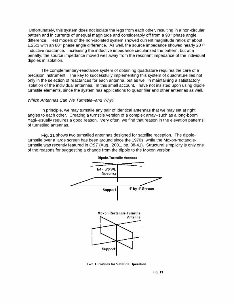
In principle, we may turnstile any pair of identical antennas that we may set at rightangles to each other. Creating a turnstile version of a complex array--such as a long-boomYagi--usually requires a good reason. Very often, we find that reason in the elevation patternsof turnstiled antennas.

Fig. 11 shows two turnstiled antennas designed for satellite reception. The dipole-turnstile over a large screen has been around since the 1970s, while the Moxon-rectangle-turnstile was recently featured in QST (Aug., 2001, pp. 38-41). Structural simplicity is only oneof the reasons for suggesting a change from the dipole to the Moxon version.

The other reason appears in Fig. 12, which presents the elevation patterns for the twoantennas at 145.9 MHz at 2 λ above ground. The Moxon shows a somewhat smoother domeof coverage at higher elevation angles. The individual Moxons have a feedpoint impedance of50 Ω, so the overall system feedpoint impedance is 25 Ω. A 1/4-λ section of 35-Ω cable(possible composed of parallel sections of 70-Ω cable if RG-83 is not handy) transforms theimpedance to 49 Ω for a standard coaxial main feedline.

One limiting factor of a dipole-turnstile for point-to-point communications in omni-directional service is the relatively modest gain: about 4.7 dBi when the antenna is 1 λ aboveground. We can increase the gain by a full dB if we turnstile quad loops instead of dipoles. Fig. 13 shows the outlines of such an arrangement, but without the phaseline. Whencomposed of #14 copper wire for 50.5 MHz, the individual quad loops have an impedance of125 Ω, and a phaseline made from RG-63 is ideal. The net system feedpoint impedance isabout 62 Ω, for a very wide-band 50-Ohm SWR of about 1.25:1.

The improvement of the quad-turnstile over its dipole cousin involves more than gain. Fig. 14 shows elevation patterns for both a dipole-turnstile and a quad-turnstile with their bases1 λ above ground. At first sight, the quad elevation pattern seems normal, with the lower lobebeing stronger than the second elevation lobe. However, notice the beam width of the secondlobe. Now examine the dipole-turnstile pattern. With the simpler turnstile, the strongest lobe isactually the one with the higher elevation angle. Not only is the gain slightly higher than for thelower lobe, but as well, the higher-angle lobe has a wider beamwidth.

The dipole and quad elevation patterns should arouse some suspicions concerning thedirection of strongest radiation relative to the structure of a turnstile antenna. As well, the utilityof the turnstile for satellite reception should add to our suspicions. The simplest way to resolvethe issue is to place a dipole-turnstile model in free space and examine the resulting pattern.

Fig. 15 shows a free-space elevation pattern or H-plane pattern for our 50.5-MHz dipoleturnstile. I have superimposed a sketch of the antenna to ensure that we orient ourselvescorrectly to the pattern. The dipole-turnstile has a higher gain broadside to the dipole pair thanit does edgewise, the orientation we use for omni-directional coverage. The difference in gainis well over 3 dB. Only ground reflections allow us to achieve a usable amount of gain at a lowelevation angle when we place the antenna over real ground.

The quad-turnstile improves both the gain and the elevation pattern by virtue of its form. It consists of two dipoles stacked 1/4 λ apart vertically, with the ends bent to meet. Essentially,we feed the two dipoles in phase. Any two dipoles stacked vertically and fed in phase will tendto suppress some high-angle radiation, with consequent increases in low angle radiation. However, the 1/4-λ spacing is not ideal if our goal is to suppress as much of the high angleradiation as possible. A spacing of 1/2 λ is superior, but has a few pitfalls if we do not designour new array carefully.

Stacking Dipole-Turnstiles

Fig. 16 shows the outline of two dipole-turnstiles stacked 1/2 λ apart. For ourexamination, we shall place the lower array at 1 λ above ground, with the upper array at 1.5 λ.

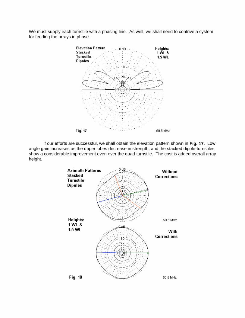
We must supply each turnstile with a phasing line. As well, we shall need to contrive a systemfor feeding the arrays in phase.

If our efforts are successful, we shall obtain the elevation pattern shown in Fig. 17. Lowangle gain increases as the upper lobes decrease in strength, and the stacked dipole-turnstilesshow a considerable improvement even over the quad-turnstile. The cost is added overall arrayheight.

With many antennas, stacking at a distance of 1/2 λ requires only that we take ouroriginal antennas and set them the proper distance apart. However, the dipole-turnstile showsvery high levels of radiation both up and down. If we stack our 111.5" dipole system with its 70-Ω phaselines, we shall likely be disappointed. The upper portion of Fig. 18 shows why. Theresulting pattern displays considerable distortion relative to the desired omni-directional pattern. In fact, the differential between maximum and minimum gain is over 3.8 dB. This situationwould not show up well in mere SWR curves, since the feedpoint impedance for each array isabout 37.1 Ω, very close to the value of individual turnstile dipole pairs.

Table 5 shows the reason why we obtain such a distorted pattern. Within each dipole-turnstile, the current magnitude ratio and phase angle differentials are far from ideal. What wehave neglected to take into account is the relatively strong mutual coupling between the dipolesin each array of the stack. The mutual coupling will alter the required element lengths and alsothe required phaseline characteristic impedance.

Perhaps the simplest way to account for the mutual coupling is to create a stack of twosimple dipoles in a model. Each dipole will be in its final position relative to the eventual stackof turnstiles, that is, 1 λ and 1.5 λ above ground. Now we can adjust the element lengths toobtain resonance. Under these conditions, we obtain a resonant length of 114.7" (0.491 λ),with individual feedpoint impedances of 62.2 - j 0.5 Ω (bottom) and 63.4 + j 0.9 Ω. Not only willour stacked dipole-turnstile array need longer elements, as well, it will need a 63-Ω phaseline. Modeling such a line is simpler than constructing one, although we might well parallel sectionsof RG-63 (125 Ω Zo) for the requisite impedance.

Stacked Dipole-Turnstile Arrays at 1/2 λ

A. Casual Version: each dipole length 111.5" (0.477 λ)Position Dipole 1 Dipole 2 I Ratio Phase I Mag. I Phase I Mag. I Phase Diff.Bottom 0.620 18.39 0.530 -93.33 1.170 111.72Top 0.612 17.50 0.529 -93.35 1.157 110.85

B. Careful Version: each dipole length 114.7" (0.491 λ)Position Dipole 1 Dipole 2 I Ratio Phase I Mag. I Phase I Mag. I Phase Diff.Bottom 0.521 -1.35 0.500 -89.73 1.042 88.38Top 0.512 -2.24 0.500 -90.19 1.024 87.95

Table 5. Current magnitudes and phase angles for casual and careful stacks of dipole-turnstiles 1/2 λ apart.

The current conditions for our revised stack of dipole-turnstile arrays appears in thelower part of Table 5. The current ratio between elements in each turnstile is much closer tothe ideal value of 1.0, and the relative phase angles are within about 2E of ideal. The lowerportion of Fig. 18 shows the effects of our work upon the azimuth pattern. The gain variationtotals just about 1 dB, with a maximum gain of about 8.4 dBi. We have gained nearly 4 dBrelative to a single dipole-turnstile and nearly 3 dB over the quad-turnstile array, all with a veryacceptable pattern for virtually any omni-directional purpose.

The feedpoint impedance for each array is very close to 31.5 Ω. A pair of 50-Ω lines,each 3/4 λ long will yield a parallel impedance of about 40 Ω. However, for this case, we mightwish to use a Regier series match. A 0.037 λ section of 93-Ω cable (RG-62) followed by a0.165 λ section of 50-Ω cable (RG8/58) would yield a 93-Ω line impedance. Once we includethe velocity factors, we can create a short, straight pair of matching lines to a Tee junction for a46-Ω impedance to the main feedline.

Conclusion

The turnstile array is, like all phased arrays, dependent upon the relative currentmagnitude and phase angle on each element for proper operation as an omni-directionalhorizontally polarized antenna. We have examined a number of conditions of construction andof operation that create distorted azimuth patterns, as well as correctives we might apply torestore near-ideal patterns. Among the conditions we explored were impedance-basedcombined matching and phasing systems, which led to the consideration of numerousalternatives that do not affect the desired antenna pattern.

We also looked at a number of candidate antennas for turnstiling, as well as why theypromised certain types of performance. Except for satellite operation, where we wish toenhance the vertical field, most omni-directional operations seek increased low-angle radiation. While the quad-turnstile offers some improvement with simple construction, stacked dipoleturnstiles offer the most improvement. However, the very factor that led us to stack turnstiles--ahigh level of radiation vertically or perpendicular to each turnstile element pair--required us toredesign the stack elements to account for mutual coupling among elements, withconsequential changes in the required phaselines.

The turnstile antenna turns out not to be nearly so simple an antennas as we mightimagine it to be. However, the better we understand its place among phased arrays, the morewe may be able to exploit its potentials.

Appendix

The Relationship of Dipole-Turnstile Azimuth Patterns to Relative Current Magnitude andPhasing of the Dipole Elements

A well-constructed dipole-turnstile antenna consists of 2 dipoles at right angles. For thisdiscussion, Dipole 1 will designate the element at the center of which we find the systemfeedpoint and the beginning of the phaseline. Dipole 2 will be the element at the far end of thephaseline. Ideally, the two dipoles will show currents of equal magnitude (a 1:1 ratio of currentsfrom Dipole 1 to Dipole 2). Dipole 2 will show a net phase difference of 90E relative to dipole 1. It does not matter operationally whether Dipole 2 is +90E or -90E relative to Dipole 1. However,for consistency in this discussion, we shall use +90E as the ideal phase difference.

Under ideal phasing conditions, the azimuth pattern of a dipole-turnstile will be nearlycircular. We cannot eliminate the pattern flattening between 90E points on the compass due tolimitations of beamwidth of the dipoles making up the array. Under ideal conditions, thedifferential in gain between points of maximum radiation and points of minimum radiation will beabout 0.9 to 1.0 dB.

There is a systematic relationship between azimuth pattern properties and the degree towhich the dipoles depart from ideal phasing conditions. A given dipole-turnstile may have aless-than-ideal current ratio between dipoles or a relative phase angle that is greater or lessthan 90E--or a combination of both. As we move either variable away from ideal, the gaindifferential between maximum and minimum values increases and is a useful marker of thedegree of azimuth pattern distortion.

Fig. 19 graphs the gain differential in azimuth patterns for the two variables. As withother 50.5 MHz dipole-turnstiles used in these notes, the antenna is 1 λ above ground. Therange of current ratios from Dipole 1 to Dipole 2 is 0.75 to 1.25 in linear steps of 0.05. Theupper region above a 1:1 ratio of current magnitude becomes a smaller percentage differenceand hence yields a shallower curve than the ratios below 1:1. Relative phase angle incrementsare 10E from 70E to 110E.

As is evident from the graph, a 90E phase angle between the currents on the dipolesyields the shallowest curve with the least distortion. Notably, the two curves that represent 10Edepartures from the ideal overlay each other, as do the two curves representing 20E departuresfrom ideal. Equal departures from the ideal phase angle above and below that level result inequally great distortions to the azimuth pattern when the relative current magnitude ratio is thesame. However, the pattern shapes will differ.

Fig. 20 shows azimuth patterns for a current ratio of 0.75. In viewing the patterns,consider Dipole 1 to extend vertically through the center of the graph, with Dipole 2 extendinghorizontally. Because the current on Dipole 2 is higher, patterns will be distended vertically andpinched horizontally. At a relative phase angle of 90E, the pattern is symmetrical, with a gaindifferential of about 2.5 dB.

With the same current ratio, relative phase angles above and below 90E will bend orpush the azimuth pattern as indicated in Fig. 20. At first sight, the patterns appear to be bi-directional ovals. However, the higher-gain portions of the patterns are not symmetrical about acenter line. Instead, the current ratio yields an offset in peak gain in a broadside directionrelative to the dipole with the higher relative current magnitude.

Fig. 21 presents comparable information for the situation in which Dipole 1 (a verticalline for each plot grid) has a current magnitude that is 1.25 times that on Dipole 2 (a horizontalline). With a phase angle of 90E, we obtain the same symmetry shown in Fig. 20, but at rightangles to the earlier pattern. Phase angles of 70E and 110E yield distorted bi-directionalpatterns with the peak gain once more nearly broadside to the dipole with the higher current.

For a 20E phase angle error and a 25% offset in the ideal current ratio, pattern distortionyields 4 dB or more differential between maximum and minimum gain. The level of patterndistortion is serious relative to a desire for omni-directional horizontally polarized coverage. However, this level of distortion is not difficult to obtain under conditions of haphazard dipole-turnstile construction or operation. As with any phased array, turnstile performance will be afunction of the care with which we establish the conditions of correct current phasing betweenthe elements.

Copyright ARRL (2002), all rights reserved. This material originally appeared in QEX: Forum forCommunications Experimenters, Mar, 2002, pp. 35-46 (www.arrl.org/qex). Reproduced with permission.