sources of particulate matter in the athabasca oil sands
TRANSCRIPT

Sources of Particulate Matter in the Athabasca Oil Sands
Region: Investigation through a Comparison of Trace
Metal Measurement Techniques
by
Catherine Danielle Phillips-Smith
A thesis submitted in conformity with the requirements for the degree of MASc
Department of Chemical Engineering and Applied Chemistry University of Toronto
© Copyright by Catherine Danielle Phillips-Smith 2015

ii
Sources of Particulate Matter in the Athabasca Oil Sands Region:
Investigation through a Comparison of Trace Metal Measurement
Techniques
Catherine Danielle Phillips-Smith
Masters of Applied Science
Department of Chemical Engineering and Applied Chemistry
University of Toronto
2015
Abstract
The province of Alberta is home to three oil sands regions which, combined, contain the third
largest deposit of oil in the world. Of these, the Athabasca Oil Sands Region is the largest. In
conjunction with Environment Canada’s Joint Canada-Alberta Implementation Plan for Oil
Sands Monitoring program, concentrations of trace metal(oid)s in PM2.5 were measured during a
long-term filter campaign and a short-term, semi-continuous measurement, campaign. The data
from the two campaigns were analysed individually using positive matrix factorization. Seven
emission sources of PM2.5 were thereby identified: two types of Upgrader Emissions, Soil, Haul
Road Dust, Biomass Burning, and two sources of mixed origin. Overall, most of the PM2.5
related metal(oid)s was found to be anthropogenic, or to be aerosolized through anthropogenic
activities. These emissions may in part explain the elevation of metals in the snow, water, and
biota previously reported for samples collected near the oil sands operations.

iii
Acknowledgments
This study was undertaken with the financial and operational support of the Government of
Canada through the federal Department of the Environment. Infrastructure support was provided
by the Canada Foundation for Innovation and the Ontario Research Fund (Project: 19606).
This study would not have been possible without the support of the members of SOCAAR. In
particular, Cheol Heon-Jeong, Robert M. Healy, and Greg G. Evans.
This study would not have been possible without the help of members of the Canadian
Government’s Department of the Environment such as Jeff Brook, Ewa Dabek-Zlotorzynska,
and Valbona Celo.

iv
Table of Contents
Acknowledgments .......................................................................................................................... iii
Table of Contents ........................................................................................................................... iv
List of Tables ................................................................................................................................. vi
List of Figures ................................................................................................................................ ix
Chapter 1 Introduction .................................................................................................................... 1
1 Background of Athabasca Region .............................................................................................. 1
2 Environmental Effects of Bitumen Extraction ........................................................................... 1
3 Study Goals ................................................................................................................................ 3
Chapter 2 Methods .......................................................................................................................... 5
1 Field Measurement Sites ............................................................................................................ 5
2 Instrumentation .......................................................................................................................... 7
2.1 Filter Campaign Setup ........................................................................................................ 7
2.2 Semi-Continuous Measurement Campaign Setup .............................................................. 8
2.3 Miscellaneous Measurements ............................................................................................. 9
3 Quality Control and Quality Assurance ................................................................................... 10
4 Data Analysis ........................................................................................................................... 18
4.1 Positive Matrix Factorization ............................................................................................ 18
4.2 Supporting Analyses ......................................................................................................... 26
Chapter 3 Results and Discussion ................................................................................................. 29
1 Species Trends ......................................................................................................................... 29
2 PMF Results ............................................................................................................................. 31
2.1 Upgrader Emissions I ........................................................................................................ 37
2.2 Upgrader Emissions II ...................................................................................................... 39
2.3 Soil .................................................................................................................................... 40

v
2.4 Haul Road Dust ................................................................................................................. 43
2.5 Biomass Burning ............................................................................................................... 43
2.6 Mixed Sources .................................................................................................................. 44
3 Spatial and Temporal Trends ................................................................................................... 47
4 Filter vs. Semi-Continuous Study Sampling ............................................................................ 63
5 Implications of the Source Identification for the Metal Species .............................................. 65
Chapter 4 Conclusions and Recommendations ............................................................................. 67
1 Conclusions .............................................................................................................................. 67
2 Recommendations .................................................................................................................... 68
Bibliography ................................................................................................................................. 69
Appendices .................................................................................................................................... 76
1 Pearson’s Coefficient Sample Calculation ............................................................................... 76

vi
List of Tables
Table 1: Description of the measurement strategy used during the two campaigns. Both
campaigns utilized EDXRF and ICP-MS to analyze filter samples: the filter campaign took 24-hr
filter samples once every three days for two years as well as 23-hr filter samples every day for a
month. Augmenting these measurements, the filter campaign measured the Lanthanoid metals
species collected in the filters, while the semi-continuous measurement campaign used a semi-
continuous XRF instrument, the Xact625, to take hourly measurements of a smaller set of metals.
......................................................................................................................................................... 8
Table 2: Uncertainties, energy levels, accuracies, and precisions of the metal analysis by the
Xact625 used for the PMF analysis of the semi-continuous measurement campaign. In contrast to
the filter concentration comparisons, overall the metals measured by the Xact625 display
reasonable accuracy and precision with their metal standards. Exceptions to this are the precision
of S at the higher concentrations, the accuracy of Ca, and the accuracy and precision of Ni at the
higher concentrations. Further insight into the cause of the deviations between the high and
medium metal standards may prove useful in explaining the different relations seen across the
high, medium, and low concentration metals seen in Figure 4, Figure 5, and Figure 6. .............. 17
Table 3: Minimum detection limits, S/N ratios, and average values of metals measured by the
Xact625 and analyzed using PMF. Overall the average value of each metal measured during the
semi-continuous measurement campaign is higher than its MDL. Metals whose average values
are below their MDL typically displayed more uncertainty, which lowered the S/N ratio. This
was largely due to the high quantity of measurements below or near the MDL. ......................... 19
Table 4: Standard deviations of the Q-factor across 150 PMF runs for the semi-continuous
measurement and filter campaigns. In addition to Figure 9, this method provides researchers with
an idea of how stable each factor solution is. After identifying the range of factors that are most
likely to contain the best solution through identifying the inflection point, those factor solutions
can be analyzed for stability. Once the relative stabilities of the possible solutions are identified,
each possibility can be analyzed based on how physically meaningful they are. It is possible for a
solution with more factors than the most stable, central option to be the most physically

vii
meaningful, which may suggest that there is a not enough data for that to be the most statistically
stable solution. .............................................................................................................................. 23
Table 5: Average concentrations of elements used in the PMF analysis of the Filter Campaign
average and 90th percentile (Dec. 2010-Dec. 2012, Aug. 2013) for all three sites compared to
average metal concentrations in Halifax, St John, Montreal, Windsor, Toronto, Edmonton, and
Vancouver (Environment Canada, 2015). All metal(oid)s are measured either by acid digested
ICP-MS (1) or ED-XRF (2). Based on this comparison, Athabasca Region has higher metal
concentrations of Si, Ti, K, Fe, Ca, and Al than the cities on average. In its highest peaks S, Ba,
Br, and Mn also surpasses the concentrations typically seen in the cities. ................................... 30
Table 6: Diversity values for the metals analyzed in the semi-continuous measurement and filter
campaigns. Species in bold had diversity values greater than 3.5 and thus were too diverse to be
used to distinguish between factors. From this table, most metals can be used as tracer species in
identifying possible sources of the various factors. ...................................................................... 32
Table 7: Details the Gasses (Obtained from WBEA) that are correlated with the different factor
time series. r is the Pearson’s correlation, and the p value for the student’s T test. ..................... 35
Table 8: Details the aerosols that are correlated with the different factor time series. r is the
Pearson’s correlation, and the p value for the student’s T test. .................................................... 35
Table 9: Enrichment factors of the 5 factors identified through PMF: Al/Fe; Si/Fe; K/Fe; Ca/Fe;
Ti/Fe. From this table it can be seen that the enrichment factors of soil and road dust between are
mostly around 1. This suggests that these elements are not elevated beyond natural levels through
anthropogenic means. ................................................................................................................... 42
Table 10: Factor Profiles for the semi-continuous measurement campaign’s Upgrader Emissions
I and the Main Upgrader Stack. The first column displayed the concentration values (g/g) of the
calculated Upgrader Emissions I factor while column 2 displays the concentration (g/g) of the
average sample taken from Upgrader stacks in the area. .............................................................. 76
Table 11: Calculation of parameters used to calculate r. First, the difference between each data
point and the average value of all the data points in that column is found (column 3 and column
6). Afterwards, that value is squared (column 4 and column 7). These values are added together

viii
then their square root is calculated. Finally the values in column 3 and column 6 are multiplied
together (column 8). These values are then added together. ......................................................... 76

ix
List of Figures
Figure 1: Locations of the various extraction processes and measurement sites within the
Municipality of Wood-Buffalo in the Athabasca Region of Alberta, Canada. The three sites;
AMS13-Fort McKay South: AMS11-Lower Camp: and AMS5-Mannix, are north of Fort
McMurray, are all near open pit mines, upgrading facilities, paved roads, and off-road traffic
operated by three different oil sands companies: Suncor, Syncrude, and CNRL. Map courtesy of
Alberta: Environmental and Sustainable Resource Development. Available:
http://osip.alberta.ca/map/. .............................................................................................................. 6
Figure 2: Comparison of Pd rod concentration to the three measured upscale metals: Cr, Cd, and
Pb that were measured throughout the campaign. The three metals: Cr, Cd, and Pb, each
represent the group of metals in energy level 1, energy level 2, and energy level 3, respectively.
Each line represents the correction applied to the metal concentrations measured after Aug. 25,
2013 within each energy level. Energy Level 1 encompasses Si, S, K, Ca, Ti, V, Cr, Mn, and Ba.
Energy Level 2 encompasses Fe, Co, Ni, Cu, Zn, As, Se, Br, Rb, Sr, Hg, and Pb. Energy Level 3
encompasses Pd, Ag, Cd, and Sn. ................................................................................................. 12
Figure 3: a) Comparison of SP-AMS sulphur equivalent to Xact625 S before Aug. 25, 2013 b)
comparison of SP-AMS sulphur equivalent to raw Xact625 S data after Aug. 25, 2013 and c)
comparison of SP-AMS sulphur equivalent to corrected Xact625 S data after Aug. 25, 2013. All
the SP-AMS sulphate values were divided by three to determine equivalent sulphur mass values.
Prior to Aug. 25, 2013, the Xact625 S data has a high relation (r2=0.95), but over-predicts the
SP-AMS concentration by a multiplication factor of 2.75. After Aug. 25, 2013, the raw data is
much closer to the SP-AMS sulphate data (1.60), but the r2 value is lower (0.92). After
correction, the r2 value is much higher than that of the raw data (0.98), but the slope of the line
(3.57) is even higher than it was before Aug. 25, 2013, suggesting that the upscale energy
correlation seen in Figure 2 may have been an over-correction. .................................................. 13
Figure 4: Filter-Xact625 comparison for metals with average concentrations <10 ng/m3. The
slope of the line between the Xact625 measurements and the filter samples (1.03), as well as its
high correlation (r2=0.95), suggests that within this bracket, the Xact625 accurately measures
metals in comparison to what can be measured by filter techniques. ........................................... 14

x
Figure 5: Filter-Xact625 comparison for metals with average concentrations >10 ng/m3 and
<50ng/m3. The slope of the line between the Xact625 measurements and the filter samples
(0.77), and its high correlation (r2=0.99), suggests that within this bracket, the Xact625 may be
under-predicting what can be measured by filter techniques. However, as there was only one
metal in this bracket that had any data points to compare, this may not be the case for other
metals in this bracket. ................................................................................................................... 14
Figure 6: Filter-Xact625 comparison for metals with average concentrations >50ng/m3. The
slope of the line between the Xact625 measurements and the filter samples (1.43), and its high
correlation (r2=0.99), suggests that within this bracket, the Xact625 may be over-predicting what
can be measured by filter techniques in this bracket. ................................................................... 15
Figure 7: AIM-IC/Xact625 comparison for Sulphur before Aug. 25, 2013. The slope of the line
between the Xact625 measurements and the filter samples (1.42), and its high correlation
(r2=0.84), suggests that within this bracket, the Xact625 may be over-predicting what can be
measured by the AIM-IC. ............................................................................................................. 15
Figure 8: PM2.5 concentrations measured by the AIM-IC to PM1.0 concentrations measured by the
AMS comparison S before Aug. 25, 2013. The slope of the line between the Xact625
measurements and the filter samples (1.66), and its high correlation (r2=0.84), confirms that the
PM2.5 concentrations measured by the AIM-IC are larger than the PM1.0 concentrations measured
by the AMS. .................................................................................................................................. 15
Figure 9: Q analysis of the semi-continuous measurement and filter campaigns. Analyzing this
graph for inflection points provides researchers with a preliminary idea of how many number of
factors may be affecting the data set. For example, the overall filter (Long-Term) campaign data
(in orange) clearly displays an inflection point around 5 factors, as can be seen by the large
change in slope before and after that factor. From there, researchers can analyze solutions that
contain 4, 5, and 6 factors to determine which solution is the most physically meaningful. ....... 21
Figure 10: 5-factor solutions for 4 independently run PMF analysis of the filter campaign. Dark
blue is the overall solution run after combining the data from all three sites; green is the
independently run AMS 13 data; orange is the independently run AMS 5 data; and purple is the
independently run AMS 11 data. Overall this shows that the three independently run PMF data

xi
sets result in similar factor profiles, suggesting that the same factors independently affect each
site. From top to bottom the factors are: Biomass Burning, Soil, Haul Road Dust, Upgrader
Emissions I, and Mixed Sources. .................................................................................................. 24
Figure 11: 6-factor solutions for 4 independently run PMF analysis of the filter campaign. Dark
blue is the overall solution run after combining the data from all three sites; green is the
independently run AMS 13 data; orange is the independently run AMS 5 data; and purple is the
independently run AMS 11 data. Overall this shows that the three independently run PMF data
sets result in similar factor profiles, suggesting that the same factors independently affect each
site. From the factor profiles it is clear that in increasing the number of factors from 5 factors to 6
factors, there is no clean split of one factor into two. This renders the factors seen in the 5 factor
solution less physically meaningful, and also does not produce a new, physically meaningful,
factor. Because of this, as well as the higher stability of the 5-factor solution, the 5-factor
solution was chosen instead of the 6-factor solution. ................................................................... 25
Figure 12: Factor profiles from the semi-continuous measurement campaign measured by the
Xact625 (Cooper Environ.). The percentage of species is defined as the percentage of mass of
each metal apportioned to each factor. Elements with Shannon entropy below 3.5 have been
given a higher transparency than the remaining elements. ........................................................... 34
Figure 13: Example linear correlation between the Soil concentration time series against that of
Black Carbon, measured with an AMS (Willis, et al., 2014). ...................................................... 36
Figure 14: Factor profiles of the combined filter campaign data. Elements with Shannon entropy
below 3.5 have been given a higher transparency than the remaining elements. ......................... 37
Figure 15: Comparison of metal profiles comparing the semi-continuous measurement
campaign’s data, and the metal profiles measured in Landis, et al., 2012: Upgrader Emissions
I/Main Upgrader Stack; Upgrader Emissions II/Main Upgrader Stack; Soil/Overburden Dump;
Haul Road Dust/Haul Road Dust. From this image it is clear how closely related the factors
calculated by the Xact625 are to the samples of material collected. ............................................ 38
Figure 16: Comparison of metal profiles comparing the filter campaign, and the metal profiles
measured in Landis, et al., 2012: Upgrader Emissions I/Main Upgrader Stack; Soil/Overburden
Dump; Haul Road Dust/Haul Road Dust; Biomass Burning/Biomass Burning. From this image it

xii
is clear how closely related the factors calculated by the filters are to the samples of material
collected. ....................................................................................................................................... 40
Figure 17: Alternative 6-factor solution calculated using PMF for the semi-continuous
measurement campaign. From top to bottom the factors are Soil, Unknown 1, Unknown 2,
Upgrader Emissions I, Mixed Sources, and Unknown 3. The three unknown factors were split
from Haul Road Dust, Upgrader Emissions II, and a bit from Mixed Sources. This split did not
result in more physically meaningful results, which is why the 5-factor solution was chosen. ... 45
Figure 18: Alternative 4-factor solution calculated using PMF for the semi-continuous
measurement campaign. In order, the factors are Upgrader Emissions I, Mixed Sources,
Upgrader Emissions II + Soil, and Haul Road Dust. The combination of Upgrader Emissions II
and Soil was less stable than the 5-factor solution and did not create a more physically solution,
which was why the 5-factor solution was chosen. ........................................................................ 47
Figure 19: Concentration time series of the semi-continuous measurement campaign. ............... 49
Figure 20: Concentration time series of the filter campaign from November, 2010 to November,
2012 for AMS13, AMS5, and AMS11. ........................................................................................ 50
Figure 21: Average seasonal contribution from the combined filter campaign’s data. The
contributions are averaged by the season winter (December 21- March 19); spring (March 20-
June 20); summer (June 21-September 21), and fall (September 22-December 20). ................... 51
Figure 22: Overall and seasonal wind roses of the three sites analyzed in the filter campaign. ... 54
Figure 23: Typical average monthly temperatures for Fort McMurray, AB for the year 2010-
2011 (Government of Canada, 2010-2011). Temperatures between October and April regularly
drop below freezing, which may explain the low concentrations of Soil and Haul Road Dust
during these times. ........................................................................................................................ 55
Figure 24: Average mass contributions of each factor for Aug. 2013 for filter and Xact625
(Cooper, Environ.) data at AMS 13. The overall contributions of the Upgrader Emissions I factor
are similar across the two campaigns. ........................................................................................... 57

xiii
Figure 25: Average concentrations displaying the diurnal trends of the soil factor (grey) and the
road dust factor (black), and the average wind speeds at AMS13 between Dec., 2010 and Sept.,
2012 (Green). Both Soil and Haul Road Dust exhibit similar, slightly offset, daily trends. This
suggests that they are both a result of vehicular traffic that occurs nearly simultaneously. ......... 58
Figure 26: CPF profiles of the 5 factors identified by the semi-continuous measurement
campaign. Blue Circles indicate the location of potential sources. ‘Gaps’ in the yellow wind rose
are due to a lack of wind data coming from certain directions. The wind roses of both Upgrader
Emissions I and II indicate that the source of these factors originate in the direction of known
Upgrading Facilities. Similarly Haul Road Dust appears to originate in the direction of major
roads. Both the Soil and the Mixed Sources factors appear to originate in and around the location
of active mines. Map courtesy of Alberta: Environmental and Sustainable Resource
Development. Stand Alone Upgrader added by author. Available: http://osip.alberta.ca/map/ ... 60
Figure 27: CPF plots from all three sites; AMS13, AMS5, and AMS11 for each factor identified
using PMF ofn the filter campaign’s data. The wind roses of Upgrader Emissions I indicate that
factor originates in the direction of known Upgrading Facilities. Similarly Haul Road Dust
appears to originate in the direction of major roads. Both the Soil and the Mixed Sources factors
appear to originate in and around the location of active mines. Finally, the Biomass Burning
factor indicates this factor originates to the north and south of the Athabasca Valley. Map
courtesy of Alberta: Environmental and Sustainable . Stand Alone Upgrader added by author.
Resource Development. Available: http://osip.alberta.ca/map/ .................................................... 61
Figure 28: HYSPLIT Analysis diagrams of the 4 days with the overall highest contributions of
the Biomass Burning factor: June 2, 2011; June 14, 2011; May 27, 2011; May 21, 2011. Figure
25a and 25c both show that the 24 trend of the winds originate from one location, which pass
through the location of forest fires that occurred that day (USDA Forest Service: Remote Sensing
Applications Center, 2011). The origin of the winds in Figure 25b and 25d come from more than
one location, but all of them pass through known forest fires that occurred that day (USDA
Forest Service: Remote Sensing Applications Center, 2011). ...................................................... 62
Figure 29: HYSPLIT analysis diagrams of the 2 days with the highest overall soil contributions:
June 8, 2011; March 22, 2012. Both Figure 26a and Figure 26b show that the 24 hour winds that

xiv
reached the receptor site that day only passed through largely uninhabited regions. This indicates
that the soil factor likely comes from a more local source. .......................................................... 63

xv
List of Appendices
Appendix 1: Pearson’s Coefficient Sample Calculation…………………………………………76

1
Chapter 1 Introduction
1 Background of Athabasca Region
The Athabasca Oil Sands Region, located in the north-east corner of the province, is the largest
of the three oil sands deposits in Alberta, Canada (Bytnerowicz, et al., 2010). This area contains
an estimated 1.7 trillion barrels of oil, located tens of meters below the ground (Kean, 2009),
composed of a mixture of high viscosity, heavy molecular weight hydrocarbons: bitumen, clay,
sand, and water (Bytnerowicz, et al., 2010). As of 2009, the oil was extracted at a rate of 0.825
million barrels per day (Moritis, 2010), predominantly through two methods: open pit mining
and steam assisted gravity drainage (Canadian Association of Petroleum Producers, 2014). Open
pit mining is a two-step process that requires the removal and separate upgrading of the oil-
containing mixture, and is feasible only to depths of 75 m (Moritis, 2006). In-situ methods, such
as steam assisted gravity drainage, involve the injection of steam and light hydrocarbons into the
soil to facilitate the flow of heavy bitumen to the surface, and are the preferred methods for
extraction at depths below 75 m (Butler, 1982). Combined, these methods have rendered 10% of
the bitumen in the oil sands economically recoverable, making Alberta home to the third largest
known oil deposit in the world after Venezuela and Saudi Arabia (Xu & Bell, 2013).
2 Environmental Effects of Bitumen Extraction
The various processes involved in bitumen extraction are believed to have environmental
impacts on the area’s water (McMaster, et al., 2006), soil (Whitfield, et al., 2009), and ecology
(Goff, et al., 2013). While air quality studies are much more limited (Hodson, 2013; Bari &
Kindzierski, 2015), gaseous emissions such as SO2, O3, and NOx are known pollutants associated
with oil sands activities (Bytnerowicz, et al., 2010; Charpentier & Bergerson, 2009). These

2
gasses have been linked to several oils sands extraction processes such as mining, transportation,
and upgrading processes (Howell, et al., 2014). Of current interest are aerosol particles below 2.5
µm in diameter (PM2.5), which can affect the environment through visibility reduction and by
directly or indirectly shifting the earth’s radiation balance (Posfai & Buseck, 2010; Dusek, et al.,
2006; Jeong, et al., 2013). Further, PM2.5 has been linked to adverse health outcomes (Docker, et
al., 1993; Burnett, et al., 1995; Schlesinger, 2007) due to its propensity to penetrate deep down to
the alveolar region of the lungs (Alfoldy, et al., 2009; Borm & Kreyling, 2004). PM2.5 is
produced both by natural and anthropogenic sources such as motor vehicles, wind-blown dust,
industrial processes, and biomass burning (Jeong, et al., 2013). Past research on PM2.5 within the
Athabasca Region has included modelling (Cho, et al., 2012), airborne studies (Howell, et al.,
2014), and comparisons of the regions PM2.5 concentrations to other areas of Canada
(Kindzierski & Bari, 2011; Hsu, 2012; Kindzierski & Bari, 2012).
No previous studies have examined the metal composition of PM2.5 in this region. Compositional
analysis of PM2.5 can help elucidate sources and processes that contribute to PM2.5 mass
concentrations. The metal species in PM2.5 are of particular importance because they can be
source-specific and are typically preserved in the aerosol phase during transport. These metals
can be either present as particles, ions, or part of larger complexes, depending on the species of
metal, its emission source, and reactivity. For example, V and Ni are often indicative of oil
combustion and react to form complexes over time (Becagli, et al., 2012), while Al, K, Mg, and
Cr are indicative of road dust (Amato, et al., 2014). This source specificity allows for the
identification of sources of PM2.5 with great resolution (Moreno, et al., 2009). Receptor models
are often used to determine these sources in areas where the chemical composition of the various
sources is unknown. One such receptor model is Positive Matrix Factorization (PMF), which
uses a weighted multivariate statistical approach to identify pollution sources (called factors) by

3
examining the correlations in the PM2.5 metal speciation matrix over time. (Paatero, 1996). In
past receptor modeling, open pit mining, upgrading, and fugitive dust have been identified as
major emission factors in the oil sands region (Landis, et al., 2012). However, these emission
factors were identified based on metal species measured in lichen, which is not necessarily
representative of PM2.5.
Previous studies also provide indirect indications of elevated levels of metals in this region.
Through dry and wet deposition, such as snowfall (Bari, et al., 2014), it is possible for the metals
contained in the particulate matter to reach the soil and surface waters in the area (Amodio, et al.,
2014). Metals, such as Cu, Zn, Ni, Cr, and Pb have been found to be higher in the Athabasca
River, its tributaries, and snowpack near the oil sands developments than several hundred
kilometers away (Kelly, et al., 2010). Further, epiphytic lichens have experienced increases in Ti,
Al, Si, and Ba (Landis, et al., 2012). In summary, the available evidence suggests that metal
contamination may already be occurring in this region and that some of this may be due to
transport of metals present at elevated levels within PM2.5. It is possible that PM2.5 may
contribute to these elevations through wet and dry deposition.
3 Study Goals
Due to these gaps in knowledge, the purpose of this work is threefold: (1) To fill the knowledge
gap that exists about PM2.5 metals and source apportionment/receptor modelling applications, (2)
to assess the accuracy, precision, and consistency of the Xact625 as a measurement technique of
trace elements versus that of the more standard 24-hr filters, and (3) to determine what can be
learned from receptor modelling using higher time-resolved vs. 24-hr filter data.
Since December 2010, under the Enhanced Deposition Component of the Joint Canada-Alberta
Implementation Plan for Oil Sands Monitoring (JOSM) Program, trace elements have been

4
measured by Environment Canada in PM2.5 at three sites operated by the Wood Buffalo
Environmental Association (WBEA), in close proximity to oil sands processing activities (Figure
1). The 24-hr integrated filter samples are collected every 6 days (midnight-midnight) following
the procedure used in the National Air Pollution Surveillance (NAPS) programs. Further, as part
of the 2013 JOSM summer intensive field campaign, hourly measurements using semi-
continuous metal monitoring system in addition to daily 23-hr filter measurements were
conducted at one of the sites (Fort McKay South, AMS 13) for one month (Aug. 10- Sept. 10).
A comprehensive protocol was developed to analyze the data from each study individually with
PMF, which made it possible to identify the sources of PM2.5 affecting the measurement sites
(Sofowote, et al., 2014; Jeong, et al., 2013). The identity of these sources was supported by
comparing the resolved source profiles with existing profiles for the suspected sources along
with temporal patterns of measured gaseous species. Meteorological data (courtesy of the
WBEA) was used to further improve interpretation and identify probable source locations. By
comparing the PMF results of the 24-hr filter and hourly semi-continuous measurements, a more
thorough understanding of the long and short term temporal variability of the sources, and the
applicability of the measurement techniques to receptor modelling was achieved.

5
Chapter 2 Methods
1 Field Measurement Sites
Under the Air Component of JOSM, the Municipality of Wood-Buffalo was selected for the
monitoring of emissions associated with oil sands activities because it is home to both mining
and in situ extraction operations. In the long-term filter study, metal concentrations were
monitored around the Athabasca river valley at 3 of the WBEA air monitoring stations (AMS):
AMS 13- Fort McKay South (SYN); AMS 5- Mannix (MAN); and AMS 11- Lower Camp
(LOW) (Figure 1). The AMS 13 site is located between three oil companies in the area, all of
which perform extensive mining, upgrading, and in-situ processing (Figure 1): Canadian Natural
Resources Limited (CNRL) is to the north, Syncrude is to the south, and Suncor is to the
southeast. All three companies extract bitumen through both open pit mining and in situ methods
within the Athabasca Region. The other two measurement sites are located farther south, directly
between Syncrude and Suncor, with AMS 11 to the north of AMS 5 (Figure 1).

6
Figure 1: Locations of the various extraction processes and measurement sites within the
Municipality of Wood-Buffalo in the Athabasca Region of Alberta, Canada. The three
sites; AMS13-Fort McKay South: AMS11-Lower Camp: and AMS5-Mannix, are north of
Fort McMurray, are all near open pit mines, upgrading facilities, paved roads, and off-
road traffic operated by three different oil sands companies: Suncor, Syncrude, and
CNRL. Map courtesy of Alberta: Environmental and Sustainable Resource Development.
Available: http://osip.alberta.ca/map/.
Within the Municipality of Wood-Buffalo, open pit mining is the predominant method of
bitumen extraction. In open pit mining, large hydraulic shovels lift the bitumen-rich dirt into
trucks for transport to a nearby wet crusher which reduces the size of the soil and adds water,
allowing the soil-slurry to be piped to an upgrading facility (Syncrude Canada Ltd., 2015;
Canadian Association of Petroleum Producers, 2014). Once at the upgrading facility the bitumen
Athabasca Region
Alberta
Edmonton
Calgary
Suncor
AMS 5-
Mannix
AMS 11-
Lower Camp
Syncrude
CNRL
AMS 13-
Fort McKay
South
Fort McMurray

7
is separated from the slurry in large settling vessels, after which it is upgraded into different
hydrocarbon streams using steam, vacuum distillation, fluid cokers, and hydrocrackers
(Syncrude Canada Ltd., 2015; Canadian Association of Petroleum Producers, 2014); these
processes produce aerosol waste most of which is emitted to the air through the main upgrader
stack (Landis, et al., 2012). Other known sources of aerosol waste are caused by large fleets of
on and off-road vehicles, dust re-suspended by mining activities, evaporative emissions from
tailings ponds, and dust re-suspended from open petroleum coke piles.
2 Instrumentation
2.1 Filter Campaign Setup
PM2.5 samples were collected on 47mm PTFE membrane filters (Pall Corporation, New York)
using Thermo Fisher Partisol 2000-FRM samplers at 16.7 L/min. The samplers were operated
once every six days with a 24-hr sampling time (midnight-midnight) according to the NAPS
protocol. All samples, including laboratory, travel, and field blanks, were subjected to
gravimetric determination of PM mass and were subsequently analyzed for 22 elements using
non-destructive x-ray fluorescence (ED-XRF). PM2.5 samples were then analyzed for 37 trace
elements including 14 lanthanoids by inductively-coupled plasma mass spectrometry (ICP-MS)
combined with microwave-assisted acid digestion, which provides superior detectability for trace
metal(oids) (Celo, et al., 2011). This study applied 2-yr of filter data (Dec., 2010 to Dec., 2012)
(Table 1).
During August, 2013, PM samples were collected at the AMS 13 site using a dichotomous
sampler (Partisol 2000-D, Thermo Scientific, Waltham, MA) on 47mm PTFE filters (Pall
Corporation, New York). The sampler was operated daily with a 23-hr sampling time (8:30 am –
7:30 am). In the dichotomous PM sampler, a virtual impactor splits the incoming PM10 sample

8
stream into fine (PM2.5) and coarse (PM10-2.5) fractions. Mass flow controllers maintained the
flow rates of the fine and coarse particle streams at 15 L/min and 1.7 L/min, respectively.
Elemental composition of PM2.5 was analyzed following the procedure described above. Due to
the limited number of samples taken, this data was combined with that of the filter campaign for
PMF analysis.
Table 1: Description of the measurement strategy used during the two campaigns. Both
campaigns utilized EDXRF and ICP-MS to analyze filter samples: the filter campaign took
24-hr filter samples once every three days for two years as well as 23-hr filter samples
every day for a month. Augmenting these measurements, the filter campaign measured the
Lanthanoid metals species collected in the filters, while the semi-continuous measurement
campaign used a semi-continuous XRF instrument, the Xact625, to take hourly
measurements of a smaller set of metals.
Campaign Measurement Type AMS 5 AMS 11 AMS 13
Filter (Dec. 2010- Dec
2012)
24-hr Filters ICP-MS, EDXRF ICP-MS, EDXRF ICP-MS, EDXRF
(Aug. 2013) 23-hr Filters N/A N/A ICP-MS, EDXRF
Semi-Continuous (Aug.,
2013)
Semi-continuous N/A N/A XactTM625
2.2 Semi-Continuous Measurement Campaign Setup
In addition to the filter measurements, the XactTM 625 (Cooper Environmental Services, LLC,
2013) made hourly measurements of 23 metal species at AMS 13 between August 10 and
September 5. This semi-continuous instrument was installed in a trailer and sampled air through
a PM10 head fitted with a PM2.5 cyclone located 4.55 m above ground level. The Xact625 used a
two-step process. In the first step, particles were pumped through a section of
polytetrafluoroethylene (PTFE) filter tape at a flow rate of 16.7 lpm, which was regulated
through measurement of the inlet temperature and pressure. The section of filter tape was then
analyzed in the second phase, which employs an X-ray fluorescence technique similar to that of
EDXRF (2.1). In the sampling phase, X-rays at various, metal-specific, wavelengths are passed

9
through the collected particles. These X-rays then remove an electron from an inner ring of a
metal atom. This excitation causes an electron from the outer ring to replace the missing inner
electron, causing an X-ray at a longer X-ray to be released. These longer wavelength X-rays,
which are characteristic of specific metals, are then counted and converted to a mass
concentration (Cooper Environmental Services, LLC, 2013). Both the sampling and the
measurement phase occurred simultaneously, resulting in a full metal spectrum every hour.
While X-ray fluorescence is a common practice to measure metal-aerosols, the use of the
Xact625 is still relatively new (Batelle, 2012, Sofowote, et al., 2014). Additionally, there is some
concern that the similarities between the characteristic wavelengths of certain measured metals,
such as Si and S, with those of common gaseous species may lead to measurement uncertainty.
Despite this, the metals measured with the Xact625 have been largely seen to be accurate when
compared to other measured metals (Batelle, 2012).
2.3 Miscellaneous Measurements
The concentration time series of several other gaseous and particulate species were measured and
used for comparison to the factor profiles made from the measured metal species. These other
species include SO2, NO, NO2, NOx, Black Carbon, ammonium, organics, and pPAH. Of these,
SO2, NO, NO2, and NOx were measured by the WBEA, and Black Carbon, ammonium, organics,
and pPAH were measured during the semi-continuous measurement campaign as part of the Air
Component of JOSM. Overall, these extra gaseous and particulate species provided important
insight into the identity of the different factors.
Site selection for both campaigns at established WBEA continuous measurement sites allowed
for comparison between data measured as a part of the Air Component of JOSM against those
measured by the WBEA. Of the various species measured by the WBEA, SO2, NO, NO2, and

10
NOx proved to be the most related to the various factors identified using the metal aerosol
species. At the various WBEA continuous measurement sites, SO2 is measured using pulsed
fluorescence gas analyzers (Percy, 2013). These analyzers were run with a range of 0 to 1000
ppb, and had a minimum detection limit (MDL) between 0.5 and 1 ppb, depending on the
individual AMS site (Percy, 2013). The nitrogen species, NO, NO2, and NOx, were measured
using a Chemiluminescence gas analyzer (Percy, 2013). The ranges used for these instruments
were from 0 to either 500 or 1000 ppb, depending on the site. The MDL of these instruments are
between 0.5 to 1 ppb (Percy, 2013).
Both a soot particle aerosol mass spectrometer (SP-AMS) (Willis, et al., 2014) and a
combination of: a photo-electric aerosol sensor, a diffusion charger, an Aethalometer, and a
continuous particle counter (Polidori, et al., 2008) were deployed as part of the semi-continuous
measurement campaign. Through use of intra-cavity infrared laser vaporization and electron
impact ionization, refractory Black Carbon-containing particles and non-refractory species
associated with refractory Black Carbon are simultaneously measured by the SP-AMS (Willis, et
al., 2014). This allows for the measurements of species such as Black Carbon, ammonium, and
organics (Willis, et al., 2014). The combination of a photo-electric aerosol sensor, a diffusion
charger, an Aethalometer, and a continuous particle counter, allowed for the characterization of
particle-bound polycyclic aromatic hydrocarbons (pPAH) by determining the relative fraction of
nuclei versus accumulation mode particles (Polidori, et al., 2008).
3 Quality Control and Quality Assurance
The integrated (filter) measurements were carried out in accordance with the standard operating
protocols that were in place and care was taken to ensure that quality assurance and control
programs (ISO17025 accredited) were followed.

11
The Xact625 incorporates several Quality Assurance and Quality Control measures. With each
measurement the instrument takes, it simultaneously measures the concentration of a Pd rod that
is located within the instrument to ensure measurement stability (Batelle, 2012). Additionally,
every day at midnight, the instrument completes several tests. In one of these tests, the Xact625
measures the concentrations of metals located within an upscale rod made of Pd, Pb, Cr, and Cd.
The three metals, Pb, Cr, and Cd, in the upscale rod represent each energy level the instrument
(Batelle, 2012). When the instrument is operating under normal conditions, these measurements
are constant with each test. This feature was valuable during the August, 2013 campaign when
there was a drop in the internal Pd measurement values between August 25 and September 2,
2013. As this had the potential to alter the measured metal concentrations, the changing Pd
upscale value was linearly regressed against the upscale values of Cr, Pb, and Cd, which were
found to have slopes of 0.63, 8, and 3.3, respectively (Figure 2). These relationships were
assumed to be the same for all metals within that energy level, and measurements made August
25 to September 2 were then adjusted assuming a constant ratio between the upscale metal, and
the various metals within its energy level. To validate this assumption, a linear comparison of the
sulphur (S) data before, as well as both the raw and corrected S data during the incident was
compared to the collection-efficiency corrected PM1.0 SO4 data measured by a soot particle
aerosol mass spectrometer SP-AMS (Willis, et al., 2014); the AMS sulphate was divided by
three to determine the equivalent sulphur mass. Prior to August 25 the slope of the line was 2.75
(Figure 3); a slope greater than 1.0 was expected given that PM2.5 and PM1.0 mass values were
being compared. However, the slope of 2.75 was greater than expected due to the difference in
size cutpoints alone. For example, comparison of the ambient ion monitor ion chromatograph’s
(AIM-IC) PM2.5 to the AMS’s PM1.0 sulphate data yielded a slope of 1.66 (Figure 8), which
suggested that there is 66% more sulphate in PM2.5 than in PM1.0. The difference in the slopes of

12
2.75 vs 1.66 implied that the Xact625 might be measuring additional sulphur that was not in the
form of sulphate. However, comparison of the Xact625 sulphur with PM2.5 filter data, as
described below, indicated that the Xact625 sulphur values may be 40% too high. Thus, most of
the difference between these slopes was believed to have been due to inaccuracy in the Xact625
sulphur data. As described below, the accuracy of most other metals determined by the Xact625
was much better than that for sulphur.
Correcting the Xact625 S data for Aug 25-Sept 2 based on the concentration-dependent
equations seen in Figure S1 raised the r2 value from 0.92 to 0.98, and changed the slope of the
line from 1.60 to 3.57 (Figure 3). The large change in the slope of the line from 2.75 before
August 25 to 3.57 could have been due to an increase in sulphate size distribution. It is more
likely that the data after August 25, 2013 may have been over corrected by up to 20%. This
represented 35% of the total Xact625 data used in the PMF analysis.
Figure 2: Comparison of Pd rod concentration to the three measured upscale metals: Cr,
Cd, and Pb that were measured throughout the campaign. The three metals: Cr, Cd, and
Pb, each represent the group of metals in energy level 1, energy level 2, and energy level 3,
respectively. Each line represents the correction applied to the metal concentrations
measured after Aug. 25, 2013 within each energy level. Energy Level 1 encompasses Si, S,
K, Ca, Ti, V, Cr, Mn, and Ba. Energy Level 2 encompasses Fe, Co, Ni, Cu, Zn, As, Se, Br,
Rb, Sr, Hg, and Pb. Energy Level 3 encompasses Pd, Ag, Cd, and Sn.
y=8x-11,000
r2=0.9
y=3.3x+200
r2=0.97
y=0.63x-78
r2=0.88

13
Figure 3: a) Comparison of SP-AMS sulphur equivalent to Xact625 S before Aug. 25, 2013
b) comparison of SP-AMS sulphur equivalent to raw Xact625 S data after Aug. 25, 2013
and c) comparison of SP-AMS sulphur equivalent to corrected Xact625 S data after Aug.
25, 2013. All the SP-AMS sulphate values were divided by three to determine equivalent
sulphur mass values. Prior to Aug. 25, 2013, the Xact625 S data has a high relation
(r2=0.95), but over-predicts the SP-AMS concentration by a multiplication factor of 2.75.
After Aug. 25, 2013, the raw data is much closer to the SP-AMS sulphate data (1.60), but
the r2 value is lower (0.92). After correction, the r2 value is much higher than that of the
raw data (0.98), but the slope of the line (3.57) is even higher than it was before Aug. 25,
2013, suggesting that the upscale energy correlation seen in Figure 2 may have been an
over-correction.
A comparison of the 1-hr instrumentation data against the coincident 23 -hr filter data was
conducted to ensure the data measured with the Xact625 (Cooper, Environ.) was equivalent to
that measured with the filters. The 1-hr data was averaged between 8:30 am and 7:30 am to
correspond with the period during which the filter sample was taken. Any averaged values that
were below the detection limit (DL), or calculated using data more than 50% of which were
below the DL, were removed. The data was then divided into three groups: low, medium, and
high concentrations. Low-concentration metals, those with average values <10 ng/m3 (Figure 4),
exhibited excellent agreement, with a linear slope of 1.03 and an r2 value of 0.95 (Xact625 to
Filter data). This represented 63% of the metals measured by the Xact625 used in the PMF
analysis. The medium-concentration metals, those with averages between 10 ng/m3 and 50 ng/m3
(Figure 5), had a slope of 0.77 and an r2 of 0.99, while the high-concentration elements, such as

14
sulphur, with averages above 50 ng/m3, had a slope of 1.43 and an r2 of 0.99 (Figure 6). The
sulphur data was also linearly regressed against the SO4 data measured with an ambient ion
monitor ion chromatograph (AIM-IC), which was divided by three to estimate the S equivalent
concentration (Markovic, et al., 2012). The result was a line with a slope of 1.42 and an r2 of
0.84 (Figure 7), this further indicated the likely presence of a 40% bias in then Xact625 sulphur
measurements.
Figure 4: Filter-Xact625 comparison for metals with average concentrations <10 ng/m3.
The slope of the line between the Xact625 measurements and the filter samples (1.03), as
well as its high correlation (r2=0.95), suggests that within this bracket, the Xact625
accurately measures metals in comparison to what can be measured by filter techniques.
Figure 5: Filter-Xact625 comparison for metals with average concentrations >10 ng/m3 and
<50ng/m3. The slope of the line between the Xact625 measurements and the filter samples
(0.77), and its high correlation (r2=0.99), suggests that within this bracket, the Xact625 may
be under-predicting what can be measured by filter techniques. However, as there was only
one metal in this bracket that had any data points to compare, this may not be the case for
other metals in this bracket.

15
Figure 6: Filter-Xact625 comparison for metals with average concentrations >50ng/m3. The
slope of the line between the Xact625 measurements and the filter samples (1.43), and its
high correlation (r2=0.99), suggests that within this bracket, the Xact625 may be over-
predicting what can be measured by filter techniques in this bracket.
Figure 7: AIM-IC/Xact625 comparison for Sulphur before Aug. 25, 2013. The slope of the
line between the Xact625 measurements and the filter samples (1.42), and its high
correlation (r2=0.84), suggests that within this bracket, the Xact625 may be over-predicting
what can be measured by the AIM-IC.
Figure 8: PM2.5 concentrations measured by the AIM-IC to PM1.0 concentrations measured
by the AMS comparison S before Aug. 25, 2013. The slope of the line between the Xact625
measurements and the filter samples (1.66), and its high correlation (r2=0.84), confirms
that the PM2.5 concentrations measured by the AIM-IC are larger than the PM1.0
concentrations measured by the AMS.

16
After the instrument was returned to the laboratory, all metal standards were run to assess the
accuracy, precision, and uncertainty of each metal. High-concentration metal standards, between
7650 and 40852 ng/cm2 in concentration, were initially run for each metal between 3 and 7
times, and each metal was found to have an accuracy and precision in the range of 98-113% and
0.3-17%, respectively (Table 2). The metal-specific analytic uncertainty was then calculated
based on the sum of the average ratio of the difference between the target (T) and measured (X)
values of each run (α) divided by the target value multiplied by the total number of runs (A), the
uncertainty of the flow rate accuracy, set to be 10%, and additional metal-specific uncertainties
(M), as seen in Equation 1. If the resulting uncertainty of any metal was less than 10%, it was
raised to 10%; if there was no metal standard available for a measure metal, it was assigned an
uncertainty based on the average uncertainties of the rest of the metals in the corresponding
energy level. The results of this can be seen in Table 2.
Equation 1: uncertainty calculation
Concerns that the high concentration metal standards were unrepresentative of the metal
concentrations witnessed throughout the campaign led to a secondary test of 6 medium-
concentration metal standards; S, V, Ba, Fe, Zn, Ni (Table 2). These metal standards, chosen as
they represented all 3 energy levels of the Xact625, ranged in value from 490 ng/cm2 to 2010
ng/cm2, were much closer to the instrument’s measurements during the campaign (between 0.1
and 1300). Based on these medium standards the metal analysis by the Xact625 was estimated to
have accuracies in the range of 93-113% and precisions in the range of 0.2%-9.5% (Table 2),
which was similar to those seen in the high concentration metal standards.

17
Table 2: Uncertainties, energy levels, accuracies, and precisions of the metal analysis by the
Xact625 used for the PMF analysis of the semi-continuous measurement campaign. In
contrast to the filter concentration comparisons, overall the metals measured by the
Xact625 display reasonable accuracy and precision with their metal standards. Exceptions
to this are the precision of S at the higher concentrations, the accuracy of Ca, and the
accuracy and precision of Ni at the higher concentrations. Further insight into the cause of
the deviations between the high and medium metal standards may prove useful in
explaining the different relations seen across the high, medium, and low concentration
metals seen in Figure 4, Figure 5, and Figure 6.
High Concentration Metal
Standards
Medium Concentration
Metal Standards
Element Energy
Level
Accuracy (measured
value/target
value*100%)
Precision (95% CI/target
value*100%)
Accuracy (measured
value/target
value*100%)
Precision (95%
CI/target
value*100%)
Uncertainty (%)
Si 1 14
S 1 98 12 108 9.5 12
K 1 12
Ni 2 113 17 102 0.3 18
Ca 1 108 1 16
Cd 3 99 7 10
Se 2 99 1 10
Mn 1 101 4 10
Ti 1 102 4 10
V 1 104 4 93 3.7 11
Cr 1 104 0.5 11
Fe 2 100 2 106 0.2 10
Cu 2 99 2 10
Zn 2 102 0.3 113 1.9 10
Br 2 11
Sr 2 10
Despite the variations in the slopes that the high, medium, and low concentration metals
exhibited when compared to the co-measured filter samples, the r2 values were high (over 0.95)
(Figure 4, Figure 5, and Figure 6). This, in addition to the results from the high and medium
metal standards led to the conclusion that the concentrations measured by the Xact625 were
precise and largely accurate for most metals. Unresolved divergence remained among the
Xact625, AIM-IC, SP-AMS, and filter measurements for some elements such as sulphur. The

18
agreement between the medium and high concentration standards indicated that this was not due
to non-linearity in the calibration.
4 Data Analysis
4.1 Positive Matrix Factorization
The metal speciation data of the two measurement methods were analyzed using Positive Matrix
Factorization (PMF). Developed by Paatero and Tapper, PMF is a least squares regression model
that inputs the data (X) and uncertainty (σ) matrices of the receptor site, resolving them into
factor profiles (F), factor contributions (G), and residuals (E) (Paatero & Tapper, 1993; 1994)
(Equation 2). Each factor corresponds to a mixture of pollution sources/processes that co-occur
when they contribute to particles at receptor site; the profile displays the concentration of metal
species within each factor, and the time series displays the normalized contribution of each factor
to the total metal concentration over time (Norris & Duvall, 2014).
Equation 2
Special consideration was given to the input data (X) and uncertainty (σ) matrices by sorting the
data into three categories: above the DL, below the DL, and missing values (Xie, et al., 1999).
Data above the DL was input directly, with an uncertainty of σij + DL/3. Data below the DL was
replaced with DL/2, and given an uncertainty of 5(DL)/6. Missing values were replaced with the
geometric mean of the measured concentrations (v), and had the highest uncertainty of the three
categories (4v) (Xie, et al., 1999). Additionally, each remaining metal species was classified as
good, weak, or bad depending on the S/N ratio (Equation 3). Metal species with an S/N ratio
above 2 were classified as good, while weak data had an S/N ratio between 0.2 and 2, and were
down-weighted by a factor of 3 (Paatero & Hopke, 2003; Norris & Duvall, 2014) (Table 3). Data

19
with an S/N ratio below 0.2 were classified as “bad” and given a weight of zero (Paatero &
Hopke, 2003). The only exception to this was Cu, which had an S/N ratio of 2.76, but was
classified as ‘weak’. This was done as all measurements that were above the DL were very close
to the DL, raising their uncertainties. Finally, the data set were all given an additional 10%
“Extra Modelling Uncertainty” to further reduce the effects of noise within the data (Norris &
Duvall, 2014).
Equation 3
Table 3: Minimum detection limits, S/N ratios, and average values of metals measured by
the Xact625 and analyzed using PMF. Overall the average value of each metal measured
during the semi-continuous measurement campaign is higher than its MDL. Metals whose
average values are below their MDL typically displayed more uncertainty, which lowered
the S/N ratio. This was largely due to the high quantity of measurements below or near the
MDL.
Element MDL (ng/m3) S/N Ratio Average Value (ng/m3)
Si 74.9 3.72 143
S 16.4 8.10 468
K 11.5 4.29 31
Ca 26.7 3.89 54
Ti 1.4 4.79 3.4
V 0.2 3.22 0.21
Cr 0.1 1.82 0.04
Mn 1.1 2.40 1.12
Fe 25.7 4.78 60
Ni 0.3 0.80 0.08
Cu 2.0 2.76 2.04
Zn 5.9 0.75 0.88
Se 0.1 1.50 0.07
Br 0.2 4.79 0.54
Sr 0.6 0.82 0.23
The goal of the PMF algorithm is to minimize the sum of squares Q value (Equation 4) (Paatero
& Hopke, 2002), which is used to determine the actual number of factors affecting the receptor
site through its stability and inflection point. Because different pseudorandom numbers are

20
selected by the algorithm at the initiation of each run, a stable solution with a preset number of
factors will not experience a change in the Q value through a series of runs (Xie, et al., 1999).
Also, since the Q value of the solution decreases with an increase in the preset number of output
factors, an inflection point in the rate of decrease will indicate the most central, or optimal,
solution (Xie, et al., 1999) (Figure 9). The optimal number of factors can also be determined by
examination of the G-space plot, a direct comparison of the time series (G matrix) of one factor
against that of another factor, and the scaled residuals of the results. Factor solutions that contain
metals with a non-normal distribution in the scaled residual could signify that the uncertainty of
the metal is too low, that there is noise in the data, or that there is another pollutant source of the
metal not separated in the factor solution (Paatero, 1996). It should also be noted that a linear
relationship between two factors in the G-space plot could signify either a co-aligned or identical
source (Paatero, et al., 2005).
Equation 4

21
Figure 9: Q analysis of the semi-continuous measurement and filter campaigns. Analyzing
this graph for inflection points provides researchers with a preliminary idea of how many
number of factors may be affecting the data set. For example, the overall filter (Long-
Term) campaign data (in orange) clearly displays an inflection point around 5 factors, as
can be seen by the large change in slope before and after that factor. From there,
researchers can analyze solutions that contain 4, 5, and 6 factors to determine which
solution is the most physically meaningful.
The final parameter examined in the selection of the optimal solution for the receptor site was the
user-specified rotational parameter, Ф, chosen for the FPEAK analysis. When the PMF
algorithm is run normally, i.e. with Ф=0, it finds the optimal solution the farthest away from any
zeros in both the G and the F matrices (Paatero, et al., 2002). When the value of Ф is changed to
lie between -2 and 2, in the FPEAK analysis, the rotation of the algorithm is altered to allow for
zeros or negative numbers in either the G or the F matrix (Paatero, et al., 2002). A stable solution
will not change radically when the rotation, Ф, is changed, but the change in rotation may
“clean” the solution by allowing the minor elements of the factor to go to zero (Paatero, et al.,
2002). Throughout this study, the value of Ф was selected to be 0.

22
The filter and the Xact625 data were analyzed separately using PMF due to their difference in
the sampling intervals. Filter data from the two time periods were combined to produce a single
data matrix. Additionally, the filter data from all three sites were combined into one data set prior
to running the PMF algorithm. The goal of this was to take advantage of the close proximity and
remote nature of the three sampling locations, assuming most, if not all aerosol sources are
common among the sites, at the expense of independent PMF solutions. The spatial variability of
the sites may also add extra factor-discriminating power, as each site is in a different direction to
the various sources. This technique succeeded in producing a stable 5-factor solution, which
were similar to the 5-factor solutions produced when the filter data from each site was run
independently (AMS 5, AMS 11, and AMS 13) (Figure 10). Not only did the 5-factor solution
exhibit the most central and stable Q factor, but also proved to be the most physically meaningful
when compared to the solutions with the 6 factor solution (Figure 11). Overall, combining the
three data sets stabilized the Q factor of the input data, as can be seen from the clear lowest
standard deviation in the filter campaign- combined filters versus the individual sites’ standard
deviations (Table 4).

23
Table 4: Standard deviations of the Q-factor across 150 PMF runs for the semi-continuous
measurement and filter campaigns. In addition to Figure 9, this method provides
researchers with an idea of how stable each factor solution is. After identifying the range of
factors that are most likely to contain the best solution through identifying the inflection
point, those factor solutions can be analyzed for stability. Once the relative stabilities of the
possible solutions are identified, each possibility can be analyzed based on how physically
meaningful they are. It is possible for a solution with more factors than the most stable,
central option to be the most physically meaningful, which may suggest that there is a not
enough data for that to be the most statistically stable solution.
Number of
Factors
Semi-
Continuous
Campaign
Filter
Campaign-
Combined
Filters
Filter
Campaign
AMS13
Filter
Campaign-
AMS5
Filter
Campaign-
AMS11
3 0.3 270 93 0.02 71
4 22 31 52 110 0.2
5 0.4 27 18 6.8 0.1
6 0.5 41 14 24 15
7 1.9 150 5.5 13 31
8 11 57 5.5 27 32
9 160 5.6 21 8.7
10 100 5.4 47 11
11 36 5.2 48 11
12 100 5.3 32 9.6
13 19 5.3 26
In order to determine the relative weights of the different factors, as well as render their results
more meaningful, a multiple linear regression of the time series of each factor for both
campaigns was run against both the summed metal concentrations as well as the PM2.5
concentration (obtained from WBEA). As trace metals only account for a small percentage of the
overall PM2.5 mass, the results of the PM2.5 regression proved to be a poor fit both statistically
(r2<0.8) and physically, as it resulted in negative relative weights, to the metal speciation factor
solutions. Because of this, the total metals concentration was used to determine the relative
weights of the different factors, which resulted in a much better fit (r2>0.99), and could then

24
convert the factor profile and time series to units of ngMetal/ngTotal_Metal and ngMetal/m3,
respectively.
Figure 10: 5-factor solutions for 4 independently run PMF analysis of the filter campaign.
Dark blue is the overall solution run after combining the data from all three sites; green is
the independently run AMS 13 data; orange is the independently run AMS 5 data; and
purple is the independently run AMS 11 data. Overall this shows that the three
independently run PMF data sets result in similar factor profiles, suggesting that the same
factors independently affect each site. From top to bottom the factors are: Biomass
Burning, Soil, Haul Road Dust, Upgrader Emissions I, and Mixed Sources.
Fa
cto
r C
on
cen
tra
tio
n (
ng/m
3)

25
Figure 11: 6-factor solutions for 4 independently run PMF analysis of the filter campaign.
Dark blue is the overall solution run after combining the data from all three sites; green is
the independently run AMS 13 data; orange is the independently run AMS 5 data; and
purple is the independently run AMS 11 data. Overall this shows that the three
independently run PMF data sets result in similar factor profiles, suggesting that the same
factors independently affect each site. From the factor profiles it is clear that in increasing
the number of factors from 5 factors to 6 factors, there is no clean split of one factor into
two. This renders the factors seen in the 5 factor solution less physically meaningful, and
also does not produce a new, physically meaningful, factor. Because of this, as well as the
higher stability of the 5-factor solution, the 5-factor solution was chosen instead of the 6-
factor solution.
Fa
cto
r C
on
cen
tra
tio
n (
ng/m
3)
26
4.2 Supporting Analyses
To further investigate the results, linear regression analyses were performed for each factor time
series against NO, NO2, NOx, and SO2 concentrations (obtained from the Wood Buffalo
Environmental Association) in order to identify relationships. The time series of each factor
resulting from both campaigns were run through a conditional probability function (CPF) to
determine the most likely direction of the relevant sources. As described in Equation 5, the CPF
is the ratio between the number of times the mass contribution surpasses a certain threshold
percentile (95%) when the wind comes from a certain direction (mΔϴ) and the number of times
the wind came from that direction (nΔϴ) (Kim & Hopke, 2004). In this study, the wind direction
(obtained from the Wood Buffalo Environmental Association) was divided into 60 bins, each
encompassing 15°, and time periods with wind speeds below 1 m/s were removed. Given the
varied topography within the Athabasca River Basin, favouring transport of local emissions
along the river valley, the CPF only gave approximate indications of the source directions.
Additionally, HYSPLIT analysis was run on potential non-local factors.
Equation 5
In order to further examine the results of the PMF analysis, the factor time series were regressed
against several aerosol species including Black Carbon, ammonium, organics (Willis, et al.,
2014), and pPAH (Polidori, et al., 2008). Correlation of the factors with these species would
elucidate which larger concentration aerosols are grouped into the factors: this not only aided in
identification of the sources of the individual factors but also indicated the other possible health
and environmental impacts of the factors. For example, Black Carbon is commonly associated

27
with burning and is related to several environmental impacts such as the albedo reduction of
Arctic snow packs.
To help determine which metal species were key in identifying the sources of specific factors,
Shannon entropy was used. Shannon entropy is a theoretical measure of the uncertainty
associated with a random variable (Healy, et al., 2014). Shannon entropy was used to quantify
how each species was partitioned across various factors. The bulk population diversity (Di) for
each species (i) was determined based on the mass fractions of each species (pa) for each factor
(a) across the total number of factors (A) (Healy, et al., 2014). A species equally distributed
across all five factors would have a diversity of 5: a species with a value of 1 is considered to be
entirely distributed to single factor. Overall, Shannon Entropy is an information-theoretic
measure that has been previously used to indicate biodiversity (Whittaker, 1965), genetic
diversity (Rosenburg, et al., 2002), and economic diversity (Attaran, 1986). More recently,
Shannon entropy has been used to analyze how chemical species present in particles are
distributed in an aerosol population (Healy, et al., 2014; Reimer & West, 2013). In this study,
Shannon entropy was used to analyze how the metals species were distributed across the various
factors. A metal species with a diversity value above 3.5 was considered to be equally
distributed, and, therefore, that species could not be used as a characteristic species for factor
identification.
Equation 6
Finally, Pearson product-moment correlation coefficient, r, was calculated to determine the
strength and direction of association between two ranked variables (Equation 7). This is a
parametric relation that is defined by the covariance of the variables divided by the product of

28
their standard deviations. To calculate it, xi and yi are the paired values, and n is the total number
of data points. A sample calculation of Pearson’s rank order correlation can be seen in Appendix
1.
Equation 7

29
Chapter 3 Results and Discussion
1 Species Trends
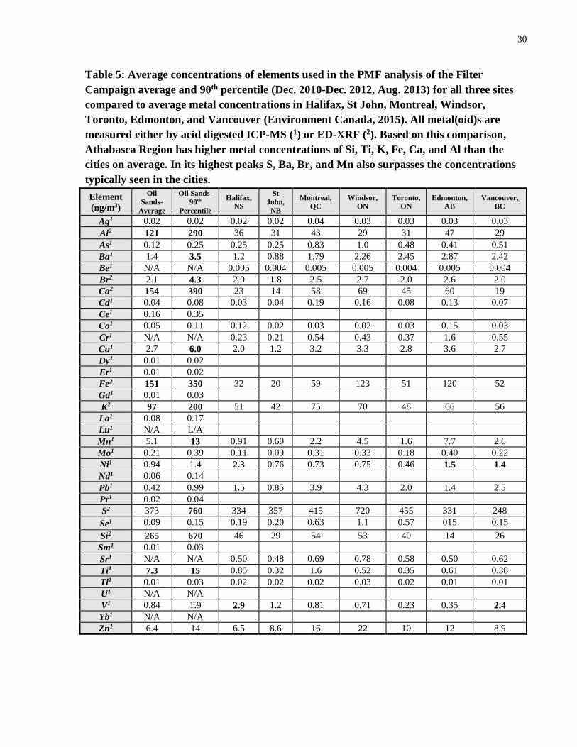
Average metal concentrations from the filter data were compared to measurements taken by the
Canadian National Air Pollution Surveillance (NAPS) network at seven different Canadian cities
(Environment Canada, 2015) (Table 5). Prior to averaging blank values were removed as
described in Supplementary S.2, and BDL values were replaced by half the detection limit.
Overall, the average concentrations of some of the metals measured through the filter campaign
were lower than those observed in the Canadian cities (Table 5). This is not overly surprising as
these cities are impacted by a range of anthropogenic activities such as heavy traffic and
industrial factories. What was surprising were the number of metals measured in the oil sands, a
largely unpopulated location, that exhibited similar concentrations to those seen across the
various cities. In particular, levels of Si, Ti, K, Fe, Ca, and Al appeared to be elevated near the
oil sands operations. However, these averages do not fully encapsulate the differences between
the cities and the oil sands region. In the oil sands, large swaths of forest are broken up by the
occasional mine or upgrader. When the wind comes from one of these directions, particularly the
upgraders, there is a noticeable difference in the air quality. This is in contrast to a city where
levels fluctuate more regularly. To address this large variability, the 90th percentile of the various
metals was calculated and compared to the averages of the various cities. The results of this
showed that at its highest peaks, the previously discussed elevated metals further surpass the
average city values. Additionally, at the highest peaks the concentrations of S, Ba, Br, and Mn
also surpass those typically seen in the cities.
30
Table 5: Average concentrations of elements used in the PMF analysis of the Filter
Campaign average and 90th percentile (Dec. 2010-Dec. 2012, Aug. 2013) for all three sites
compared to average metal concentrations in Halifax, St John, Montreal, Windsor,
Toronto, Edmonton, and Vancouver (Environment Canada, 2015). All metal(oid)s are
measured either by acid digested ICP-MS (1) or ED-XRF (2). Based on this comparison,
Athabasca Region has higher metal concentrations of Si, Ti, K, Fe, Ca, and Al than the
cities on average. In its highest peaks S, Ba, Br, and Mn also surpasses the concentrations
typically seen in the cities.
Element
(ng/m3)
Oil
Sands-
Average
Oil Sands-
90th
Percentile
Halifax,
NS
St
John,
NB
Montreal,
QC
Windsor,
ON
Toronto,
ON
Edmonton,
AB
Vancouver,
BC
Ag1 0.02 0.02 0.02 0.02 0.04 0.03 0.03 0.03 0.03
Al2 121 290 36 31 43 29 31 47 29
As1 0.12 0.25 0.25 0.25 0.83 1.0 0.48 0.41 0.51
Ba1 1.4 3.5 1.2 0.88 1.79 2.26 2.45 2.87 2.42
Be1 N/A N/A 0.005 0.004 0.005 0.005 0.004 0.005 0.004
Br2 2.1 4.3 2.0 1.8 2.5 2.7 2.0 2.6 2.0
Ca2 154 390 23 14 58 69 45 60 19
Cd1 0.04 0.08 0.03 0.04 0.19 0.16 0.08 0.13 0.07
Ce1 0.16 0.35
Co1 0.05 0.11 0.12 0.02 0.03 0.02 0.03 0.15 0.03
Cr1 N/A N/A 0.23 0.21 0.54 0.43 0.37 1.6 0.55
Cu1 2.7 6.0 2.0 1.2 3.2 3.3 2.8 3.6 2.7
Dy1 0.01 0.02
Er1 0.01 0.02
Fe2 151 350 32 20 59 123 51 120 52
Gd1 0.01 0.03
K2 97 200 51 42 75 70 48 66 56
La1 0.08 0.17
Lu1 N/A L/A
Mn1 5.1 13 0.91 0.60 2.2 4.5 1.6 7.7 2.6
Mo1 0.21 0.39 0.11 0.09 0.31 0.33 0.18 0.40 0.22
Ni1 0.94 1.4 2.3 0.76 0.73 0.75 0.46 1.5 1.4
Nd1 0.06 0.14
Pb1 0.42 0.99 1.5 0.85 3.9 4.3 2.0 1.4 2.5
Pr1 0.02 0.04
S2 373 760 334 357 415 720 455 331 248
Se1 0.09 0.15 0.19 0.20 0.63 1.1 0.57 015 0.15
Si2 265 670 46 29 54 53 40 14 26
Sm1 0.01 0.03
Sr1 N/A N/A 0.50 0.48 0.69 0.78 0.58 0.50 0.62
Ti1 7.3 15 0.85 0.32 1.6 0.52 0.35 0.61 0.38
Tl1 0.01 0.03 0.02 0.02 0.02 0.03 0.02 0.01 0.01
U1 N/A N/A
V1 0.84 1.9 2.9 1.2 0.81 0.71 0.23 0.35 2.4
Yb1 N/A N/A
Zn1 6.4 14 6.5 8.6 16 22 10 12 8.9

31
2 PMF Results
Each technique identified five unique factors through PMF analysis. Comparison of these factors
led to the identification of seven distinct factors: two types of Upgrader Emissions, Soil, Haul
Road Dust, Biomass Burning, and two factors of presumably mixed origins. Three of these
factors were common, two were distinct, and the two mixed sources showed similarities between
the two techniques. The results of the PMF factor profiles (F matrix) from the two techniques
can be seen in Figure 19 (hourly data from the semi-continuous measurement campaign (August,
2013)) and Figure 20 (24-hr filter data from the filter campaign (Dec. 2010-Dec. 2012, Aug.
2013)). The diversity of the elements among the factors was examined using Shannon Entropy
(Table 6) (Healy, et al., 2014).

32
Table 6: Diversity values for the metals analyzed in the semi-continuous measurement and
filter campaigns. Species in bold had diversity values greater than 3.5 and thus were too
diverse to be used to distinguish between factors. From this table, most metals can be used
as tracer species in identifying possible sources of the various factors.
Metals Semi-Continuous
Campaign
Filter Campaign
Si 2.0 2.4
S 2.1 1.8
K 2.4 3.3
Ca 2.3 2.2
Ti 2.6 3.3
V 1.6 2.4
Cr 3.9
Mn 3.5 2.3
Fe 3.1 2.1
Ni 2.6 3.7
Cu 1.4 1.9
Zn 2.0 2.8
Se 2.2 3.6
Br 1.5 2.6
Sr 3. 5 3.6
Be 3.5
Al 2.6
Co 3.8
As 4.2
Mo 2.9
Ag 3.4
Cd 2.2
Ce 2.6
Ba 2.8
La 2.6
Pr 2.4
Nd 2.5
Sm 2.2
Gd 2.3
Dy 2.4
Er 3.2
Yb 2.4
Lu 3.2
Tl 3.0
Pb 3.4
U 3.4
Marker elements were then identified by either by (a) their high percentage and/or (b) their high
concentration. These marker elements enabled the initial attribution of these PMF factors to
probable sources. The identity of these sources was then supported by comparing, where
possible, the resolved PMF profiles with source profiles for the suspected sources along with
temporal patterns of measured gaseous species. Here the low diversity (high Shannon entropy) of

33
Ni and Se is interesting as it implies that these metals have become mixed into many of the
sources, perhaps as a result of contamination of either the filters, or the PM2.5 particles
themselves.
The overall factor profiles of the semi-continuous measurement campaign can be seen in Figure
12 and Figure 14. For the Upgrader Emissions I factor, S and Si are the most characteristic
metals, while Upgrader Emissions II is characterized by S, V, and Fe. Soil is characterized by
very crustal metals such as Si, K, Ti, and Fe, while Haul Road Dust is characterized by Ca, Mn,
and Fe. The Mixed Sources contains many possible characteristic metals, such as Cu, Zn, Br, Se,
and Sr. As these metals are not typically linked together, this factor may be a mixture of sources
that could not be properly split. In Figure 14, the Upgrader Emissions I is characterized by S,
while Biomass Burning is characterized by S and K. Soil is characterized by very crustal metals
such as Si, V, Al, and Fe, while Haul Road Dust is characterized by Si, Ca, Mn, and Fe. The
Mixed Sources contains many possible characteristic metals, such as Cu, Zn, Al, Mo, and Cd. As
these metals are not typically linked together, this factor may be a mixture of sources that could
not be properly split.

34
Figure 12: Factor profiles from the semi-continuous measurement campaign measured by
the Xact625 (Cooper Environ.). The percentage of species is defined as the percentage of
mass of each metal apportioned to each factor. Elements with Shannon entropy below 3.5
have been given a higher transparency than the remaining elements.
Supporting the results of these factors is Table 7. Table 7 displays the results of the correlation
between the factor time series of the semi-continuous measurement and filter campaigns against
co-measured gaseous species. The high correlation of SO2 to Upgrader Emissions I confirms that
this factor is due to combustion, while the high correlation of Soil and Haul Road Dust to NO2
and NOx suggests that these factors are a by-product of vehicular traffic.
Percen
tag
e of Sp
ecies
Co
ntr
ibu
tio
n o
f M
eta
l S
pe
cie
s (
g (
meta
l)/ g
(T
ota
l M
eta
l)
Upgrader Emissions I
Upgrader Emissions II
Mixed Sources
Soil
Haul Road Dust

35
Table 7: Details the Gasses (Obtained from WBEA) that are correlated with the different
factor time series. r is the Pearson’s correlation, and the p value for the student’s T test.
Campaign Factor Correlated Gasses (r>0.35, p<0.05)
Filter
Campaign
Upgrader Emissions I SO2 (r=0.52)
Soil
Haul Road Dust
Mixed Sources
Biomass Burning
Semi-
Continuous
Campaign
Upgrader Emissions I SO2 (r=0.84), NO2 (r=0.44)
Upgrader Emissions
II
SO2 (r=0.60), NO2 (r=0.40)
Soil NO2 (r=0. 63), NOx (r=0.54)
Haul Road Dust NO2 (r= 0.61), NOx (r=0.49)
Mixed Sources
These results are further supported by Table 8. In it, the high correlation of pPAH and Black
Carbon to the Soil factor suggests that this factor is due to traffic related sources. The actual
regression used to generate these results can be seen in Figure 13, where the high correlation
between these two time series indicates that a lot of the Black Carbon in the area comes from soil
aerosolized by vehicular traffic.
Table 8: Details the aerosols that are correlated with the different factor time series. r is the
Pearson’s correlation, and the p value for the student’s T test.
Campaign Factor Correlated Aerosols (r>0.35, p<0.05)
Semi-
Continuous
Upgrader Emissions I Ammonium (r=0.97), organics (r=0.64)
Campaign Upgrader Emissions
II
Ammonium (r=0.54), organics (r=0.43)
Soil Black Carbon (r=0.55), Ammonium
(r=0.36), organics (r=0.56), pPAH
(r=0.37)
Haul Road Dust Black Carbon (r=0.39), Ammonium
(r=0.46) , organics (r=0.60)
Mixed Sources organics (r=0.46)
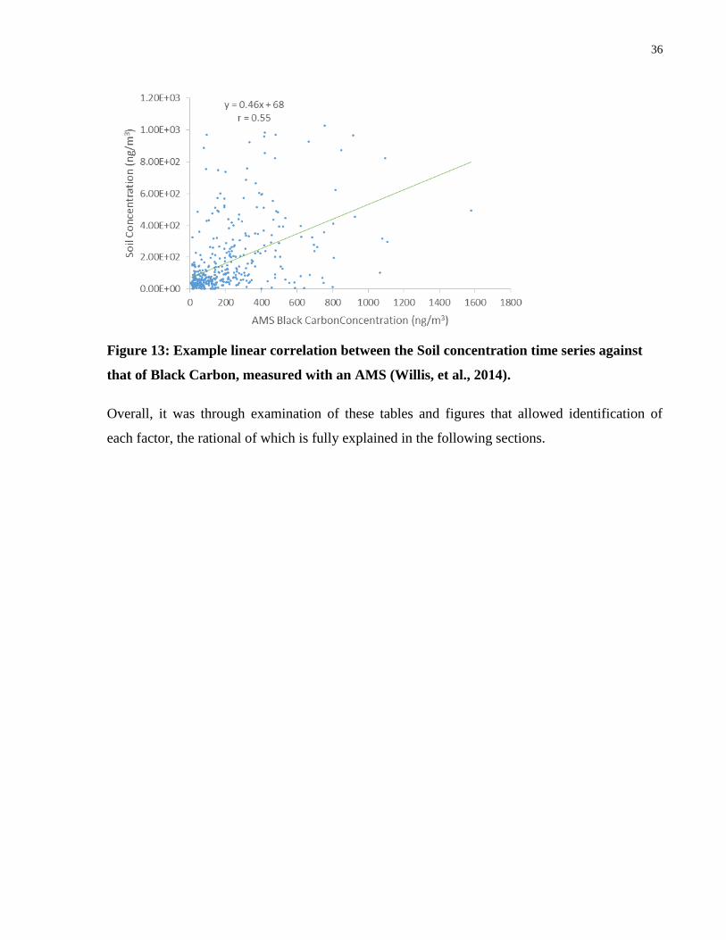
36
Figure 13: Example linear correlation between the Soil concentration time series against
that of Black Carbon, measured with an AMS (Willis, et al., 2014).
Overall, it was through examination of these tables and figures that allowed identification of
each factor, the rational of which is fully explained in the following sections.

37
Figure 14: Factor profiles of the combined filter campaign data. Elements with Shannon
entropy below 3.5 have been given a higher transparency than the remaining elements.
2.1 Upgrader Emissions I
This factor was attributed to typical emissions from the upgrading processes based on the
correlation (r=0.999, p<0.05 for the semi-continuous measurement campaign (Figure 15):
r=0.998, p<0.05 for the filter campaign (Figure 16) of its elemental profile with an average
profile derived from samples of PM2.5 taken from main upgrader stacks in the area (Landis, et al.,
2012). Specifically, the elemental profile contained significant portions of the S, V, As, Br, and
Pb. The very high S contribution in its profiles distinguished it from the second upgrader related
Pe
rcen
tag
e o
f Sp
ecie
s
Co
ntr
ibu
tio
n o
f M
eta
l S
pe
cie
s (
g (
meta
l)/ g
(T
ota
l M
eta
l)
Upgrader
Emissions I
Mixed
Soil
Haul Road
Dust
Biomass
Burning
Pe
rce
nta
ge
of
Sp
eci
es
Pe
rce
nta
ge
of
Sp
eci
es
Pe
rce
nta
ge
of
Sp
eci
es

38
factor. The profile is suggestive of a mixed-combustion source as these characteristic elements
have been previously seen in No.4 boiler fuels, a mix still used in many parts of Canada (Lee, et
al., 2000; Van Loo & Koppejan, 2008), or from S blown off of a suphur pile. However, the high
correlation of this factor with SO2 (Table 7) was consistent with the elevated SO2 observed in
fresh industrial plumes in the area (Hsu, 2012; Zhang, et al., 2015), as well as combustion,
indicating this factor is likely not a result of windblown S. This factor was also correlated with
NO2, ammonium, and organic aerosol species (Table 7 and Table 8). The PMF factor profiles
between the two campaigns and time series between the co-measured Xact625 and filter data
(profile (r=0.9987, p<0.05); time series (0.8731, p<0.05)). Combined, these observations support
the assertion that this factor resulted from combustion of a range of fuels in support of upgrading
processes.
Upgrader Emissions I
Upgrader Emissions II
Mixed Sources
Soil
Haul Road Dust
Figure 15: Comparison of metal profiles comparing the semi-continuous measurement
campaign’s data, and the metal profiles measured in Landis, et al., 2012: Upgrader
Emissions I/Main Upgrader Stack; Upgrader Emissions II/Main Upgrader Stack;
Soil/Overburden Dump; Haul Road Dust/Haul Road Dust. From this image it is clear how
closely related the factors calculated by the Xact625 are to the samples of material
collected.
Co
ntr
ibu
tio
n o
f M
eta
l S
pec
ies (
g (
meta
l)/
g (
To
tal
Me
tal)
39
2.2 Upgrader Emissions II
This factor was hypothesized to be a less common type of emissions originating from upgrading
processes; it was only resolved through the semi-continuous measurement campaign. More
specifically, this factor was attributed to oil combustion because of the elevated percentages of V
and Ni, (Figure 12), which are typical of oil combustion (Huffman, et al., 2000; Lee, et al.,
2000). Other metals associated with oil combustion such as S, Ti, Zn, and Fe (Huffman, et al.,
2000; Lee, et al., 2000) were also evident. The temporal correlation of this factor to SO2 in the
semi-continuous campaign suggested the combustion of high sulphur fuel (Table 7) (Van Loo &
Koppejan, 2008; Zhang, et al., 2015). Correlation (r=0.904, p<0.05) between the chemical
profile for this factor and the average metal profile seen in upgrader stacks around the region
(Figure 16) (Landis, et al., 2012) was not as strong as for the Upgrader Emissions I factor.
Further, the time series of this factor exhibited short-term peaks that occurred during the semi-
continuous campaign at different times than those of the first upgrader emissions factor. The
different mole ratios of particulate sulphur to SO2 (Upgrader Emissions I: 0.44, Upgrader
Emissions II: 0.22) evaluated during these short-term peaks suggested that while both sources
were relatively local, Upgrader Emissions II may have been closer to the receptor site. This, in
addition to the small contribution of this factor relative to that of the first upgrader factor,
indicated that this factor may have been due to occasional smaller plumes that occurred too
rarely to be differentiated through the long-term filter data. This is because the nature of the 24 -
hr filter data only results in the filter samples being impacted by the mixture of emissions coming
from the various particle sources around the, or associated with, upgrading area in the facilities.
In contrast, the Xact625 data’s time resolution allows for the occasional isolation of a more-
specific process/emission occurring as part of the upgrading processes, such as oil combustion
for heat/energy or the burning of coke. In this case the upgrader emissions factor for the filter

40
campaign would have included the Upgrader Emissions II factor. A less likely, but more
fortuitous, possibility is that the Upgrader Emissions II factor was due to a short-term change in
upgrader fuel that occurred only during the semi-continuous campaign.
2.3 Soil
The Soil factor exhibited high concentrations of crustal elements such as Si, Ti, and K (Figure 12
and Figure 14). Additionally, both the filter and the semi-continuous measurement campaigns’
chemical profiles exhibited a high correlation with samples taken of the area’s overburden dump
Co
ntr
ibu
tio
n o
f M
eta
l S
pe
cie
s (
g (
meta
l)/ g
(T
ota
l M
eta
l)
Upgrader
Emissions
I
Soil
Haul Road
Dust
Biomass
Burning
Figure 16: Comparison of metal profiles comparing the filter campaign, and the metal profiles
measured in Landis, et al., 2012: Upgrader Emissions I/Main Upgrader Stack;
Soil/Overburden Dump; Haul Road Dust/Haul Road Dust; Biomass Burning/Biomass Burning.
From this image it is clear how closely related the factors calculated by the filters are to the
samples of material collected.

41
(semi-continuous campaign (r=0.9882, r<0.05) (Figure 15); filter (r=0.8266, p<0.05) (Figure
16)) (Landis, et al., 2012), which supported identifying this factor as a soil factor. The
overburden dump is comprised of the top soil of the area, a mixture of the soil and glacial till
overlying the oil deposits (Landis, et al., 2012). The Soil factor from the filter campaign
exhibited high concentrations of additional crustal elements not measured in the semi-continuous
measurement campaign such as Al, and lanthanoids such as Pr, Sm, and Nd (Table 3).
Interestingly, this factor also exhibited high concentrations of Fe (both campaigns) and S (semi-
continuous campaign). In contrast, this factor was correlated with NOx, pPAH, Black Carbon,
ammonium, and organic species (Table 7 and Table 8), which was suggestive of an
anthropogenic source. To determine if this factor was primarily natural or anthropogenic in
origins, enrichment factors were calculated.
An enrichment factor is the ratio between a given metal to a reference metal in an aerosol and
that same metal to the reference metal in the source material (Equation 8) (Lawson &
Winchester, 1979). While the use and accuracy of enrichment factors have been questioned
(Reimann & De Caritat, 2000), it is understood that while an enrichment factor near 1 may or
may not be from an anthropogenic source (Lawson & Winchester, 1979; Reimann & De Caritat,
2000), an enrichment factor significantly larger than one is likely to originate from
anthropogenic sources (Lawson & Winchester, 1979). One of the most common reference metals
(Lawson & Winchester, 1979) used for enrichment factors is Fe, while some of the common
given metals (X) are Si, Al, K, Ca, and Ti (Lawson & Winchester, 1979). Accuracy of the
enrichment factors depends on the accuracy of the (X/Ref)source (Lawson & Winchester, 1979).
Equation 8

42
Table 9: Enrichment factors of the 5 factors identified through PMF: Al/Fe; Si/Fe; K/Fe;
Ca/Fe; Ti/Fe. From this table it can be seen that the enrichment factors of soil and road
dust between are mostly around 1. This suggests that these elements are not elevated
beyond natural levels through anthropogenic means.
Semi-Continuous Campaign Filter Campaign
Soil N/A;2.2;1.4;0.53;7.7 0.18;0.43;0.31;3.6;1.9
Haul Road Dust N/A;0.11;0;5.0;1.5 1.0;3.6;3.7;6.2;15
Calculation of enrichment factors, between Fe and Al, Si, K, Ca, and Ti, (Table 9) from the long-
term filter data further indicated that the origin of these metals was likely natural rather than
anthropogenic in origin (Reimann & de Caritat, 2005). Interestingly, this factor also exhibited
high concentrations of Ti, Fe and S (Figure 12, and Figure 14). This may have been due to the
presence of bitumen in the soil in the Athabasca region, or may indicate that this natural crustal
material was being aerosolized through anthropogenic means. Specifically, the soil may have
been emitted through entrainment by off-road transportation along the soil, or crushing of
bitumen-rich sand (Oil Sands Disovery Centre, 2014). This hypothesis was supported by the high
correlation of this factor with NO2 and NOx (Table 7), which are related to engine emissions
(Almeida, et al., 2014). In fact, it is probable that his Soil factor represents a combination of
emissions: (1) directly through entrainment by off-road vehicular traffic on-site and (2) indirectly
through “track-out”, where the dust temporarily sticks to vehicles travelling within the mining
sites, only to be aerosolized on-road later after leaving the site. In summary, the soil factor’s
chemical profile was consistent with natural soils but its rate of emission may have been
enhanced by anthropogenic processes. This factor was identified through both campaigns; the
source profiles and time series thereby resolved were highly correlated between the campaigns
(profile (r=0.998, p<0.05); time series (r=0.874, p<0.05)).

43
2.4 Haul Road Dust
Much like the soil factor, this factor exhibited high concentrations of crustal elements such as Ca
(Figure 12 and Figure 14), and the PMF outputs from the semi-continuous measurement and
filter campaigns were highly correlated to each other (profile (r=0.812, p<0.05); time series
(r=0.790, p<0.05)). What differentiated this factor from the soil factor were the higher
concentrations of Mn and Fe, as well as its higher correlations with NO2, NOx, ammonium, and
organic aerosol species (Figure 12, Figure 14, and Table 7), which is indicative of vehicular
traffic (Moreno, et al., 2013; Almeida, et al., 2014). In fact, the source profiles for the Soil and
Haul Road Dust were only weakly correlated (r=0.1481 p=0.629). Further, the metal profiles of
this factor were similar to that of samples taken of the Athabasca Region’s haul road dust (semi-
continuous (r=0.926, r<0.05) (Figure 15); filter (r=0.908, p<0.05) Figure 16) (Landis, et al.,
2012). As haul roads are made of a mixture of overburden material combined with limestone and
low-grade oil sand, it is reasonable that the Soil and the Haul Road Dust factors exhibit a similar
chemical composition.
2.5 Biomass Burning
Only observed in the filter campaign, this factor was characterized by its high S, K, Zn, Br, Cd,
and Pb. All of these metals, to different degrees, have been associated with different types of
biomass burning (Van Loo & Koppejan, 2008; Vassura, et al., 2014; Alves, et al., 2011) (Figure
14). Further, this combination of elements associated with different types of biomass combustion
was consistent with a forest fire (Landis, et al., 2012) in which all types of plants are burned.
Finally, this factor’s profile displayed a high correlation (r=0.885, p<0.05) with the measured
profile of an Alberta forest fire (Figure 16) (Landis, et al., 2012). Additionally, this factor
experienced a significant spike in May-June, 2011, a period of time in which there was a large

44
forest fire just north of For McKay, near the three sites (Figure 20) (USDA Forest Service:
Remote Sensing Applications Center, 2011). Combined, these similarities suggested that this
factor originated from Biomass Burning. Combined, these similarities suggested that this factor
originated from both forest fires and possibly from the scrap-brush burning that is performed by
industry in the area during the seasons with lower instances of forest fires.
2.6 Mixed Sources
The PMF results of each campaign yielded a factor that appeared to be a combination of
anthropogenic and crustal sources. While the mixed factors from the two campaign were not
correlated to each other (profile (r=0.05, p>0.80); time series (r=0.04, p>0.80)), they both
appeared to originate from multiple sources. The mixed factor from the semi-continuous
measurement campaign was characterized by elements such as Cu, Zn, and Mn, which suggested
the presence of mechanical abrasion (Zhang, et al., 2011; Gietl, et al., 2010; Bukowiecki, et al.,
2007), as well as K and Se, which suggested the inclusion of biomass or other fuel burning (Van
Loo & Koppejan, 2008; De Santiago, et al., 2014). In contrast, the marker elements from the
filter campaign were Zn, Cu, as well as K, and Ca, suggesting mechanical abrasion (Zhang, et
al., 2011; Gietl, et al., 2010; Bukowiecki, et al., 2007) and some sort of activity that would
aerosolize crustal elements as possible sources, respectively. The conflicting nature of these two
different mixed-source factors suggested the presence of further factors. This was further
evidenced by the unstable temporal trends these factors exhibited (Figure 19 and Figure 20), as
well as the relative stability of the alternate 6-factor solutions (Table 4).

45
Figure 17: Alternative 6-factor solution calculated using PMF for the semi-continuous
measurement campaign. From top to bottom the factors are Soil, Unknown 1, Unknown 2,
Upgrader Emissions I, Mixed Sources, and Unknown 3. The three unknown factors were
split from Haul Road Dust, Upgrader Emissions II, and a bit from Mixed Sources. This
split did not result in more physically meaningful results, which is why the 5-factor solution
was chosen.
As an example, some of the characteristic metals identified in the semi-continuous campaign,
such as Br and Se, proved to be less stable, and would separate from the semi-continuous
campaign’s mixed factor when the number of factors was increased (Figure 17). However, these
Fa
cto
r C
on
cen
tra
tio
n (
ng/m
3)
Fa
ctor P
ercenta
ge (%
)

46
6-factor solutions were less stable than the 5-factor solutions, and did not yield additional,
clearer, factors. This suggested that these mixed factors were a result of insufficient data that
prevented full separation into more distinct source profiles. However, this factor is distinct from
the others previously identified, as it does not collapse to join another factor when the number of
factors is decreased to 4 (Figure 18). The combination of anthropogenic and crustal metals
present in these factors could have arisen from mining-related activities such as mechanical
abrasion of excavated materials within crushers (Oil Sands Disovery Centre, 2014). Activities
such mechanical abrasion would result in a full-range of PM, from ultra-fine to coarse, part of
which would be considered as PM2.5 (Okuda, et al., 2007; Martins, et al., 2015). Interestingly,
this factor was highly correlated with organic aerosol species Table 8. It is possible that a PMF
analysis that includes a speciated organic time series may provide valuable insight into the exact
source(s) of this factor.
While the overall contribution of these factors is low and relatively constant (Figure 19, Figure
20, Figure 21), which is in part why they could not split further, it does not reflect the residuals
in the data. This factor arose due to similar trends in multiple metals, which PMF then grouped
together. Residuals are the unexplainable “extra” portions of the input metal concentrations that
cannot be grouped together with anything else. This indicates that these factors are
representations of activities in the oil sands that either do not produce a lot of PM2.5, or occur
relatively continuously.
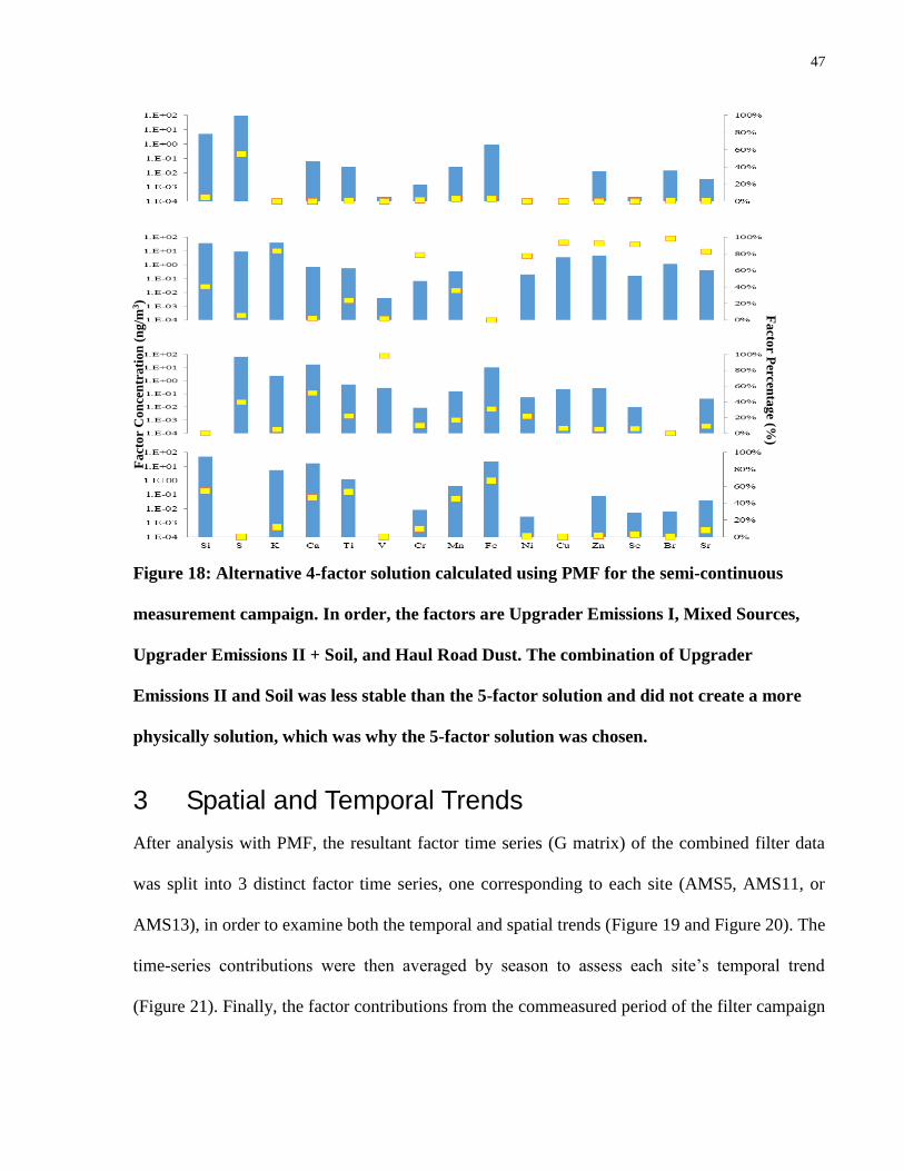
47
Figure 18: Alternative 4-factor solution calculated using PMF for the semi-continuous
measurement campaign. In order, the factors are Upgrader Emissions I, Mixed Sources,
Upgrader Emissions II + Soil, and Haul Road Dust. The combination of Upgrader
Emissions II and Soil was less stable than the 5-factor solution and did not create a more
physically solution, which was why the 5-factor solution was chosen.
3 Spatial and Temporal Trends
After analysis with PMF, the resultant factor time series (G matrix) of the combined filter data
was split into 3 distinct factor time series, one corresponding to each site (AMS5, AMS11, or
AMS13), in order to examine both the temporal and spatial trends (Figure 19 and Figure 20). The
time-series contributions were then averaged by season to assess each site’s temporal trend
(Figure 21). Finally, the factor contributions from the commeasured period of the filter campaign
Fa
cto
r C
on
cen
tra
tio
n (
ng/m
3)
Fa
ctor P
ercenta
ge (%
)

48
to the semi-continuous measurement campaign’s data measured by the Xact625 at AMS 13
(Figure 22).
Both the filter and the semi-continuous measurement campaign exhibited interesting spatial and
temporal trends which assisted in identifying the source of each factor. It is through examination
of the temporal trends seen in Figure 19 and Figure 20 that preliminary conclusions can be made
of the daily and temporal trends of each factor. In Figure 19 it can be seen that Upgrader
Emissions I and Upgrader Emissions II both displayed a very episodic nature, suggesting they
came from point source locations that only affected the receptor site when the wind was
favorable. In contrast, Soil and Haul Road Dust displayed diurnal trends, suggesting they were
due to a daily, nearby, activity such as traffic. The Mixed Sources displayed a less stable
episodic trends, suggesting that the factor may be due to a combination of more than one
different sources that could not be split.

49
Figure 19: Concentration time series of the semi-continuous measurement campaign.
It is in Figure 20 that basic seasonal trends can be seen. For example the Soil and Haul Road
Dust experienced lower concentrations in winter, which would be expected due to the freezing of
the ground in the winter. Biomass Burning was higher mostly in May to June, 2011 a period of
time in which large forest fires occurred just north of the measurement sites (USDA Forest
Service: Remote Sensing Applications Center, 2011). Mixed sources displayed a relatively
constant, unstable time series, likely due to combination of sources that combined to create the
factor. Finally, Upgrader Emissions I displayed an episodic nature typical of point sources.
Fa
cto
r C
on
cen
tra
tio
n (
ng
/m3
)

50
Figure 20: Concentration time series of the filter campaign from November, 2010 to
November, 2012 for AMS13, AMS5, and AMS11.
As can be seen from Figure 21, there were clear differences in mass loading and composition
between the three sites. Of the three sites, AMS 5 consistently exhibited the highest metal mass
concentrations, followed by AMS 11, then AMS 13, which was largely due to the high amounts
of Haul Road Dust measured at AMS 5. In contrast, AMS 11 had higher average contributions
Fa
cto
r C
on
cen
tra
tio
n (
ng
/m3
)
Biomass Burning
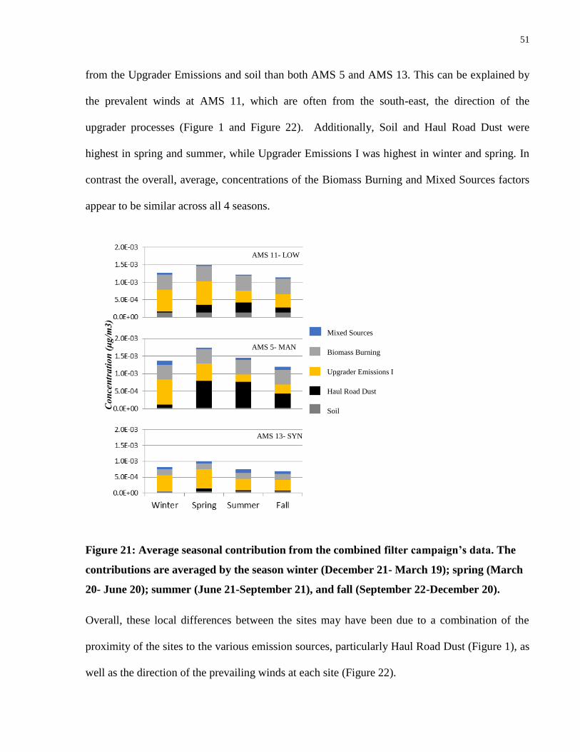
51
from the Upgrader Emissions and soil than both AMS 5 and AMS 13. This can be explained by
the prevalent winds at AMS 11, which are often from the south-east, the direction of the
upgrader processes (Figure 1 and Figure 22). Additionally, Soil and Haul Road Dust were
highest in spring and summer, while Upgrader Emissions I was highest in winter and spring. In
contrast the overall, average, concentrations of the Biomass Burning and Mixed Sources factors
appear to be similar across all 4 seasons.
Figure 21: Average seasonal contribution from the combined filter campaign’s data. The
contributions are averaged by the season winter (December 21- March 19); spring (March
20- June 20); summer (June 21-September 21), and fall (September 22-December 20).
Overall, these local differences between the sites may have been due to a combination of the
proximity of the sites to the various emission sources, particularly Haul Road Dust (Figure 1), as
well as the direction of the prevailing winds at each site (Figure 22).
AMS 5- MAN
AMS 11- LOW
AMS 13- SYN
Mixed Sources
Biomass Burning
Upgrader Emissions I
Haul Road Dust
Soil
Co
nce
ntr
ati
on
(μ
g/m
3)

52
Also seen in Figure 21 are the seasonal trends of the 5 factors identified in the filter campaign.
The total contribution was largest in the spring, then lower in the winter, then summer, then fall.
A major part of this overall trend was due to the higher contribution from Biomass Burning, a
natural source, in the spring. However, even without the inclusion of Biomass Burning, the
combined mass loading of the 4 remaining factors followed the same overall seasonal trend. Of
the 5 factors, only the mixed factor was relatively consistent throughout the seasons (within 77
ng/m3). Both the Soil and the Haul Road Dust factors were notably lower in the winter than in
the other seasons, presumably due to freezing of the ground and snow cover in the winter. The
concentrations were higher in spring than in fall. In the fall, the temperatures drop below 0°C
quickly (Figure 23), which could result in the lower Soil and Haul Road dust concentrations. In
contrast, temperatures are higher in the spring (Figure 23) and there is a surplus of sand on paved
roads from ice treatment in the winter. Interestingly, the Upgrader Emissions factor contribution
to the total PM2.5 mass was highest in the winter and spring, which may be due to the differences
in wind direction and speeds across the seasons (Figure 22), the changes in mixing height, or it
may reflect true changes in upgrader activity. Overall, the combined seasonal concentration of
the factors follows the same trend as the strength and directionality of the prevailing winds, in
which the most prevalent, fast winds are present in the spring, then winter, then summer, then
fall (Figure 22).
In addition to the wind speeds, mixing height plays a vital role in the impact of various factors
throughout the seasons. In the colder months, inversions can occur, increasing concentrations
and channeling emissions horizontally based on the local topography (Davison, et al., 1981; Celo
& Dabek-Zlotorzynska, 2010). This may result in higher contributions from emissions sources,
such as Soil and Haul Road Dust, which occur close to the ground. In contrast, in the warmer
months, more vertical mixing tends to occur (Davison, et al., 1981; Celo & Dabek-Zlotorzynska,

53
2010), which may result in the observance of higher contributions from tall emission stacks.
Thus, the seasonality apparent within the source contributions is presumably in part due to this
seasonality in mixing. However, the low contributions of the Soil and Haul Road Dust factor in
winter, when mixing is the lowest, is not likely due to low mixing, unless the mixing was so low
that it prevents transport from the sources to the nearby measurement sites. This indicates it is
more likely that emissions of Soil and Haul Road Dust are lower in winter.
AMS13-Overall
AMS13-Winter
AMS5-Overall AMS11-Overall
AMS5-Winter AMS11-Winter
<= 10 km/h
10-20 km/h
20-30 km/h
>30 km/h

54
Figure 22: Overall and seasonal wind roses of the three sites analyzed in the filter
campaign.
Figure 22 displays all the wind roses of each AMS site across each season. In these wind roses,
stronger, more direct winds may result in larger concentrations from specific sources. In contrast,
weaker winds that come from many directions may result in the smaller measurements of many
AMS13-Spring
AMS13-Summer
AMS13-Fall
AMS5-Summer AMS11-Summer
AMS5-Fall AMS11-Fall
AMS5-Spring AMS11-Spring

55
sources. Highlighting this, the predominant winds at AMS 13 came from the North and the
Southeast, which point towards the more distant CNRL and Syncrude mines. This would result
in higher concentrations of the elements in factors originating from these sources than would be
otherwise measured. In contrast, at AMS 5 the wind came from many directions in which there
were roads and open mines. This lack of directionality would result in more local sources being
present in higher concentrations.
Figure 23: Typical average monthly temperatures for Fort McMurray, AB for the year
2010-2011 (Government of Canada, 2010-2011). Temperatures between October and April
regularly drop below freezing, which may explain the low concentrations of Soil and Haul
Road Dust during these times.
A closer look at the contributions during the summer of 2013 is shown in Figure 24. The
Xact625 used in the semi-continuous measurement campaign seems to be more impacted by Soil
than the samples taken in the filter campaign, which has a higher contribution of Mixed Sources
and Haul Road Dust. This may just be due to the differences in sampling time and time ranges
that were analyzed by PMF. Only the Xact625 captured the second Upgrader Emissions factor,
while only the filters captured the Biomass Burning factor. Further, during the month of Aug.,
2013 there were no major forest fires in Canada, so this small contribution may not be an
accurate representation of Biomass Burning occurring during this time. Good agreement of the

56
Upgrader Emissions and Haul Road Dust can be seen between the PMF factor contributions
calculated from the filter and Xact625 data (17% and 19%, respectively). While there is
disagreement between the two independent PMF runs in the magnitude of the contribution from
soil, the time series for the soil factor from the filter vs semi-continuous monitoring campaign
data did exhibit good temporal correlation (r>0.87, p<0.05). The reason for this divergence is not
known but it is possible that filter data did not allow complete separation of the soil factor from
the mixed factor as the longer-time scale employed by the filter may not be able to distinguish
changes that occur on a smaller time-scale, such as the changing mixing height throughout the
day. Despite these differences in relative contributions, the factors identified by the two different
approaches were broadly similar. Finally, as the Aug. 2013 filter data was added to the rest of the
filter campaign’s data prior to analyzing it with PMF, the very small contribution (~4%) of the
Biomass Burning factor seen in this figure arose from the Biomass Burning factor resolved
through other times in the filter campaign, and given its low magnitude it is uncertain if this is an
accurate indication of emissions from biomass burning during the semi-continuous measurement
campaign.
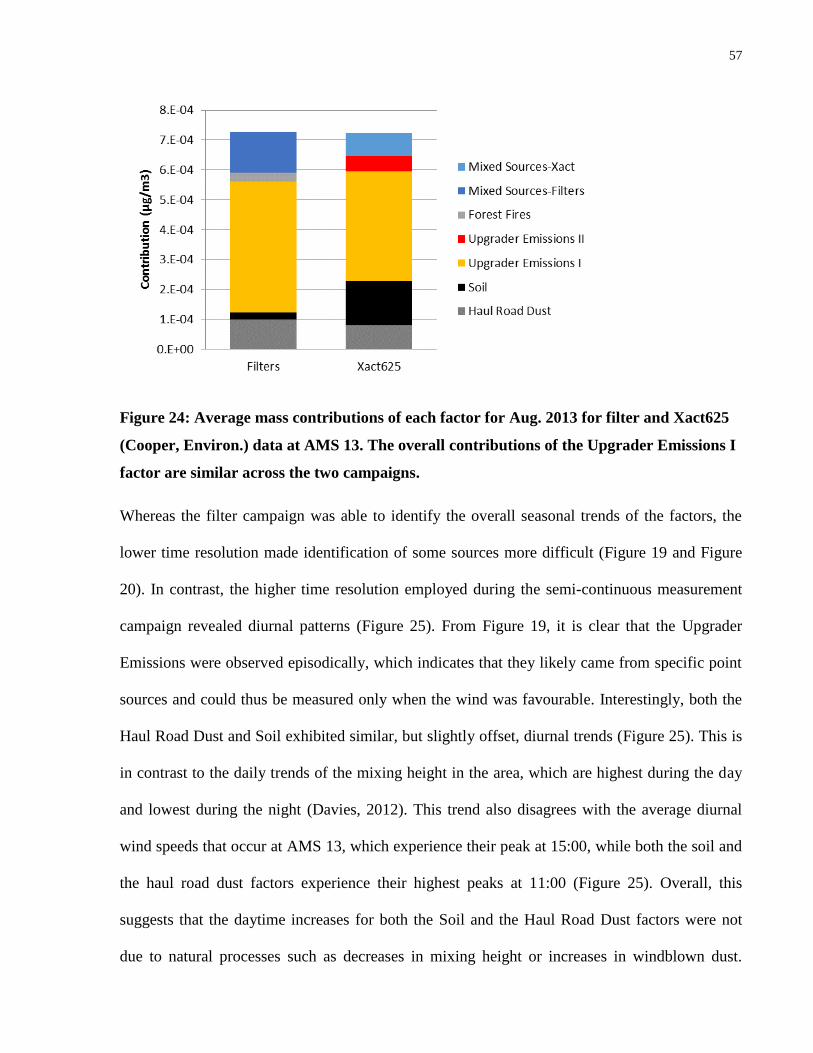
57
Figure 24: Average mass contributions of each factor for Aug. 2013 for filter and Xact625
(Cooper, Environ.) data at AMS 13. The overall contributions of the Upgrader Emissions I
factor are similar across the two campaigns.
Whereas the filter campaign was able to identify the overall seasonal trends of the factors, the
lower time resolution made identification of some sources more difficult (Figure 19 and Figure
20). In contrast, the higher time resolution employed during the semi-continuous measurement
campaign revealed diurnal patterns (Figure 25). From Figure 19, it is clear that the Upgrader
Emissions were observed episodically, which indicates that they likely came from specific point
sources and could thus be measured only when the wind was favourable. Interestingly, both the
Haul Road Dust and Soil exhibited similar, but slightly offset, diurnal trends (Figure 25). This is
in contrast to the daily trends of the mixing height in the area, which are highest during the day
and lowest during the night (Davies, 2012). This trend also disagrees with the average diurnal
wind speeds that occur at AMS 13, which experience their peak at 15:00, while both the soil and
the haul road dust factors experience their highest peaks at 11:00 (Figure 25). Overall, this
suggests that the daytime increases for both the Soil and the Haul Road Dust factors were not
due to natural processes such as decreases in mixing height or increases in windblown dust.

58
Further, the daytime increase pointed to on-road vehicles (e.g. through track-out) rather than off-
road mining activities as the more dominant source, as off-road operations at most mining sites
occur around the clock.
Figure 25: Average concentrations displaying the diurnal trends of the soil factor (grey)
and the road dust factor (black), and the average wind speeds at AMS13 between Dec.,
2010 and Sept., 2012 (Green). Both Soil and Haul Road Dust exhibit similar, slightly offset,
daily trends. This suggests that they are both a result of vehicular traffic that occurs nearly
simultaneously.
In addition to diurnal patterns, the higher time resolution used by the Xact625 resulted in more
detailed CPF plots (Figure 26 and Figure 27). Whereas the Xact625 data was able to point
towards distinct emission sources with the CPF plots, the filter data time resolution was too low.
Despite this, the multiple sites used by the filter campaign allowed for approximate triangulation
of the sources (Figure 27). The results of the two CPF profiles indicate that both the typical and
occasional Upgrader Emissions came from the direction of known upgraders and that the Mixed
factors came from the direction of known mines. The Haul Road Dust factor appeared to come
from the direction of the three major roads closest to the receptor site(s). Further, the CPF profile

59
of the soil factor exhibited broad peaks which surrounded known mines, perhaps as a results of
vehicular traffic leading to and from the mines. Finally, the Biomass Burning factor appeared to
come into the valley from the north and south. Because of this, HYSPLIT analysis was run on
the three highest-concentration days for both the Biomass Burning and the Soil factors in order
to determine if they were local, or regional, in origin. The Biomass Burning factor, which
experienced its highest concentration days during periods of known forest fires just north of the
receptor sites, appeared to largely come from consistent, specific regions in northern Alberta that
experienced additional forest fires (USDA Forest Service: Remote Sensing Applications Center,
2011) (Figure 28). Combined, the local and regional forest fires greatly affected the areas air
quality, for example the PM2.5 concentrations increased by 328%. Back trajectory analysis of the
highest concentration soil days of each receptor site suggested that it predominantly came from
the direction of known mines (Figure 29); these trajectories largely crossed uninhabited, forested,
areas in northern Canada prior to reaching the open pit mines. Overall, these finding support the
conclusions that the Upgrader Emissions came from the bitumen upgrading process, the Soil and
the Haul Road Dust factors came from on road transportation coupled with “track out”, and the
Mixed factors likely originated in the open pit mines.

60
Figure 26: CPF profiles of the 5 factors identified by the semi-continuous measurement
campaign. Blue Circles indicate the location of potential sources. ‘Gaps’ in the yellow wind
rose are due to a lack of wind data coming from certain directions. The wind roses of both
Upgrader Emissions I and II indicate that the source of these factors originate in the
direction of known Upgrading Facilities. Similarly Haul Road Dust appears to originate in
the direction of major roads. Both the Soil and the Mixed Sources factors appear to
originate in and around the location of active mines. Map courtesy of Alberta:
Environmental and Sustainable Resource Development. Stand Alone Upgrader added by
author. Available: http://osip.alberta.ca/map/
Suncor
Syncrude
CNRL
Upgrader
Emissions I
Suncor
Syncrude
CNRL
Upgrader
Emissions II
Suncor
Syncrude
CNRL
Soil
Suncor
Syncrude
CNRL
Mixed
Sources
Suncor
Syncrude
CNRL
Haul
Road Dust
Upgrader
Emissions I
Upgrader
Emissions II
I
Soil
Mixed
Sources
Haul Road
Dust
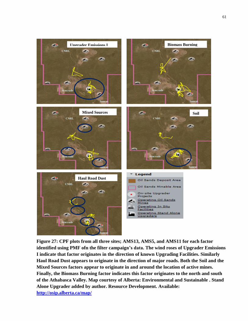
61
Figure 27: CPF plots from all three sites; AMS13, AMS5, and AMS11 for each factor
identified using PMF ofn the filter campaign’s data. The wind roses of Upgrader Emissions
I indicate that factor originates in the direction of known Upgrading Facilities. Similarly
Haul Road Dust appears to originate in the direction of major roads. Both the Soil and the
Mixed Sources factors appear to originate in and around the location of active mines.
Finally, the Biomass Burning factor indicates this factor originates to the north and south
of the Athabasca Valley. Map courtesy of Alberta: Environmental and Sustainable . Stand
Alone Upgrader added by author. Resource Development. Available:
http://osip.alberta.ca/map/
Suncor
Syncrude
CNRL
Suncor
Syncrude
CNRL Upgrader Emissions I Biomass Burning
Suncor
Syncrude
CNRL
Mixed Sources
Suncor
Syncrude
CNRL
Soil
Suncor
Syncrude
CNRL
Haul Road Dust

62
Figure 28: HYSPLIT Analysis diagrams of the 4 days with the overall highest contributions
of the Biomass Burning factor: June 2, 2011; June 14, 2011; May 27, 2011; May 21, 2011.
Figure 25a and 25c both show that the 24 trend of the winds originate from one location,
which pass through the location of forest fires that occurred that day (USDA Forest
Service: Remote Sensing Applications Center, 2011). The origin of the winds in Figure 25b
and 25d come from more than one location, but all of them pass through known forest fires
that occurred that day (USDA Forest Service: Remote Sensing Applications Center,
2011).
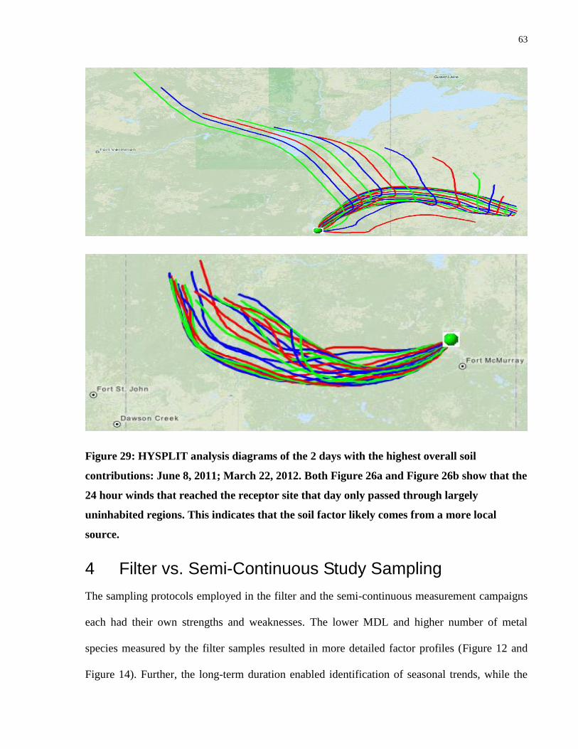
63
Figure 29: HYSPLIT analysis diagrams of the 2 days with the highest overall soil
contributions: June 8, 2011; March 22, 2012. Both Figure 26a and Figure 26b show that the
24 hour winds that reached the receptor site that day only passed through largely
uninhabited regions. This indicates that the soil factor likely comes from a more local
source.
4 Filter vs. Semi-Continuous Study Sampling
The sampling protocols employed in the filter and the semi-continuous measurement campaigns
each had their own strengths and weaknesses. The lower MDL and higher number of metal
species measured by the filter samples resulted in more detailed factor profiles (Figure 12 and
Figure 14). Further, the long-term duration enabled identification of seasonal trends, while the

64
use of multiple sampling sites improved geographic resolution of sources. However the limited
range of co-measured aerosol and gaseous species led to fewer comparisons. Additionally, the
longer sampling time employed by the filter limited the number of close proximity sources, such
as Upgrader Emissions I and II.
In contrast, the higher time resolution employed by the Xact625 (Cooper, Environ.) resulted in
better defined temporal patterns which supported the separation of similar sources (Figure 19,
Figure 20, and Figure 25), which in turn led to more precise CPF profiles and gaseous species
comparisons (Figure 26, Figure 27, and Table 7). Further, the higher time resolution
measurements accomplished all this within a much shorter time frame. However, without the
long-term filter sampling, it would have been unclear how representative this intensive period
was of the norm. Because of this, it is important to take more time-resolved metals
measurements in the area in order to see if there are further, unresolved sources. This is
important as it can help to guide decisions made about regulation and control in the area.
In addition to their measurement capabilities, each campaign had its own requirements in terms
of energy, difficulty in set up and measurement, and quality control. While the semi-continuous
measurements employed by the Xact625 had more energy and housing requirements on site, the
filter campaign required a much larger laboratory set-up. Finally, despite the quality control and
assurance measures employed by the Xact625, comparison to co-measured species indicated a
possible linear bias in certain metals measured. In contrast, the filter protocol employed is well
established, and followed stringent quality control and analysis protocols. This led to more
reliability in these measurements.
Despite their different strengths and weaknesses, both campaigns identified broadly similar
factors. However, due to the limited number of filter measurements taken during Aug. 2013,

65
independent PMF analysis based on the filter samples was not possible. In summary, these data
show that short campaign measured by semi-continuous instruments can yield some of the
knowledge derived from long-term filter sampling within a much shorter time frame, but only if
the campaign is of sufficient duration to cover a wide range of wind directions and the
occurrence of different sources.
5 Implications of the Source Identification for the Metal Species
Overall, the average concentration of some metal species measured in the Athabasca region were
either equal to or higher than those measured in urban/industrial locations in Canada (Table 5).
In particular, the concentrations of Si, Ti, K, Fe, Ca, and Al were, on average, elevated to the
point that they were higher than those measured in major Canadian cities. At its highest peaks
the concentrations of S, Ba, Br, and Mn are also higher than the city averages. Of these metals,
Ti, Fe, Cu, and Zn all showed periods of elevated concentration during the semi-continuous
measurement campaign. Of these species, Al, Ca, Si, Mn, Ba, and Fe were predominantly
observed in the Soil and Haul Road Dust factors, suggesting that they originated from vehicle-
related emissions or associated anthropogenic dust production in the area. These species have
been previously seen to be elevated in epiphytic lichens (Landis, et al., 2012). The elements As,
Pb, S, and Tl were associated with Upgrader Emissions, and Be with the Haul Road Dust; these
metals and metalloids were also previously found to be elevated in snow or biota near the oil
sands operation (Landis, et al., 2012). Overall, it is possible that some of this elevation may be in
part due to the wet and dry deposition of PM2.5.
Some metals exhibited ambiguity as to their source. Based on the filter data, V was apportioned
to Soil and Upgrader Emissions while based on the semi-continuous monitoring campaign it was

66
almost entirely apportioned to the Upgrader Emissions II factor. Likewise Br, which was seen to
be elevated at its highest peaks, was apportioned into Upgrader Emissions in the filter campaign
and Mixed Sources in the semi-continuous measurement campaign. It is likely that this
difference may be due to the difficulty the longer sampling-time employed by the filters has in
separating some sources. Further, while this difference between the campaigns does create some
ambiguity that could be resolved with further study, it is clear that V was associated with a type
of anthropogenic emissions that the filter sampling had trouble identifying.
Interestingly, Ni, Zn, Cr, Ag, and Cu were grouped into the Mixed factors. As this factor is likely
a combination of multiple sources, this suggests that the true source(s) of these elevated metals is
still not known, which may help direct further studies. The high relation this factor had with
organic aerosols suggests (Table 8) that running a PMF algorithm on both metals and speciated
organics may enable full identification of these sources.
Of the remaining metals that were previously found to be elevated in snow or biota near the oil
sands operations (Landis, et al., 2012), As, Pb, and Tl were associated with upgrader emissions,
and Be and Ba with the haul road dust. Careful control of dust and cleaning of the main upgrader
stack should assist in keeping these levels under control.
Overall, expanding oil sands mining and upgrading will likely result in further increases in metal
concentrations. This is of concern due to the toxic nature of certain metals released through
anthropogenic activities. There is also further concern as many of these anthropogenic activities
have been seen to be highly correlated with several gasses and aerosols that have their own
health and environmental impacts (Table 7, Table 8). Continued monitoring will likely be
required to understand how expansion will impact these species.

67
Chapter 4 Conclusions and Recommendations
1 Conclusions
In conjunction with JOSM, the sources of metal aerosol emissions in the Athabasca Region were
studied. Although there is still some concern as to the reliability of certain metals measured with
the Xact625, particularly sulphur which may be over estimated by 40%. While this is of concern
in order to determine the exact concentrations present in the area, the linearity between the
measurements taken by the Xact625 and those taken by filter and sulphate samples means that
this offset will not affect how the metals are split into factors through PMF.
Because of this, seven sources of PM2.5 were identified through two campaigns: two types of
Upgrading Activities; Soil; Haul Road Dust; Biomass Burning; and two sources of mixed origin.
These factors represented the larger emitters of PM2.5 related metals: of the seven factors, two
were directly associated with oil sands upgrading, two with the transportation of the bitumen-rich
oil, one with natural processes, and two with mixed anthropogenic-natural activities. Thus,
much, but not all, of the PM2.5 related metals were found to originate from anthropogenic related
sources. This is of concern due to elevation of many metals in the area, such as Ti and Si. It is
possible that it is partly through these emissions that elevations of metals in snow, water, and
biota have been observed for samples collected near the oil sands operations. Additionally, these
anthropogenic factors have been seen to be highly correlated with several gaseous and aerosol
species that have their own health and environmental impact. This is of particular concern due to
the continued expansion of extraction activities in the area.

68
2 Recommendations
Based on the results of this study, several recommendations can be drawn. First and foremost,
more work should be done to understand the measurements made by the Xact625 to see if there
are any corrections that need to be made to their measurements. This can be done through several
consecutive studies completed by different units in which the values measured by the Xact625
are compared commeasured filter and sulphate measurements.
To further understand the behaviour of the identified factors, or even further separate the mixed
sources factor, more semi-continuous measurement studies should be run not only at AMS13. As
both AMS5 and AMS11 exhibited higher concentrations of most factors, additional semi-
continuous measurement campaigns run at different times of the year would help to fill in what is
still not known about the behaviour of metals in the region.
The factor profiles can be further augmented by combining the metal data with other particulate
matter species such as sulphate, nitrate, Black Carbon and organic carbon species before re-
running it through PMF. This may even help isolate the source of Cu in the area, which is of
particular interest due to its elevation and toxic nature. Already knowing how the metals will
split on their own assist in this as it will provide the future study with an idea of when the best
number of factors has been found.
Finally, by using the updated factor profiles more accurate impact assessments of the Oil Sands
Activities can be obtained, which can be helpful in directing future studies, as well as extraction,
transportation, and upgrading methods.

69
Bibliography
Alfoldy, B., Giechaskiel, B., Hofmann, W. & Drossinos, Y., 2009. Size-distribution dependent
lung deposition of diesel exhaust particles. Journal of Aerosol Science, Volume 40, pp. 652-663.
Almeida, S. et al., 2014. Traffic-related air pollution in an industrial area. WIT Transactions on
Ecology and the Environment, Volume 181, pp. 683-694.
Alves, C. et al., 2011. Summer 2009 wildfires in Portugal; Emission of trace gases and aerosol
composition. Atmospheric Environment, Volume 45, pp. 641-649.
Amato, F. et al., 2014. Effects of road dust suppressants on PM levels in a Mediterranean urban
area. Environmental Science and Technology, 48(14), pp. 8069-8077.
Amodio, M. et al., 2014. Atmospheric deposition: Sampling procedures, analytical methods, and
main recent findings from the scientific literature. Advances in Meteorology, Volume 2014.
Attaran, M., 1986. Industrial diversity and economic performance in U.S. areas. Ann. Regional
Sci., Volume 20, pp. 44-54.
Bari, M. & Kindzierski, W., 2015. Fifteen-year trends in criteria air pollutants in oil sands
communities of Alberta, Canada. Environmental International, Volume 74, pp. 200-208.
Bari, M., Kindzierski, W. & Cho, S., 2014. A wintertime investigation of atmospheric deposition
of metals and polycyclic aromatic hydrocarbons in the Athabasca Oil Sands Region, Canada.
Science of the Total Environment, 485-486(1), pp. 180-192.
Batelle, 2012. Environmental Technology Verification Report: Cooper Environmental Services
LLC Xact 625 Particulate Metals Monitor, Portland, OR: EPA.
Becagli, S. et al., 2012. Evidence for heavy fuel oil combustion aerosols from chemical analysis
at the island of Lampedusa: A possible large role of ships emissions in the Mediterranean.
Atmospheric Chemistry and Physics, 12(7), pp. 3479-3492.
Beckhoff, B. et al., 2006. Handbook of Practical X-Ray Fulorescence Analysis. Germany:
Springer-Verlag Berlin Heidelberg.
Borm, P. & Kreyling, W., 2004. Toxicological hazards of inhaled nanoparticles-Potential
implications for drug delivery. Journal of Nanoscience and Nanotechnology, 4(5), pp. 521-531.
Bukowiecki, N. et al., 2007. Iron, manganese and copper emitted by cargo and passenger trains
in Zurich (Switzerland): Size-segregated mass concentrations in ambient air. Atmospheric
Environment, 41(4), pp. 878-889.

70
Burnett, R. et al., 1995. Associations between ambient particulate sulphate and admissions to
Ontario hospitals for cardiac and respiratory diseases. American Journal of Epidemiology,
Volume 142, pp. 15-22.
Butler, R., 1982. USA, Patent No. US 4344485 A.
Bytnerowicz, A., Fraczek, W., Schilling, S. & Alexander, D., 2010. Spatial and temporal
distribution of ambient nitric acid and ammonia in the Athabasa Oil Sands Region, Alberta. J.
Limnol, 69(1).
Canadian Association of Petroleum Producers, 2014. What are Oil Sands?. [Online]
Available at: http://www.capp.ca/canadaIndustry/oilSands/Energy-Economy/Pages/what-are-
oilsands.aspx
Celo, V. & Dabek-Zlotorzynska, E., 2010. Concentration and Source Origin of Trace Metals in
PM2.5 Collected at Selected Canadian Sites within the Canadian National Air Pollution
Surveillance Program. In: F. Zereini & C. Wiseman, eds. Urban Airborne Particulate Matter.
Berlin: Springer-Verlag, pp. 19-38.
Celo, V. et al., 2011. An improved method for determination of lanthanoids in environmental
samples by inductively coupled plasma mass spectrometry with high matrix introduction system.
Anal. Chim. Acta., Volume 706, pp. 89-96.
Charpentier, A. & Bergerson, J. M. H., 2009. Understanding the Canadian oil sands industry's
green house gas emissions. Environ. Research Letters, Volume 4.
Cho, S. et al., 2012. Emission sources sensitivity study for ground-level ozone and PM2.5 due to
oil sands development using air quality modeling system: Part 1- model evaluation for current
year base case simulation. Atmospheric Environment, Volume 55, pp. 533-541.
Cooper Environmental Services, LLC, 2013. Cooper Environmental Services, LLC. [Online]
Available at: http://cooperenvironmental.com/xact-625-monitoring-system/
[Accessed 17 09 2014].
Dabek-Zlotorzynska, E. et al., 2011. Canadian National Air Pollution Surveillance (NAPS) PM2.5
speciation program: Methodology and PM2.5 chemical composition for the years 2003-2008.
Atmospheric Environment, 45(3), pp. 673-686.
Davies, M., 2012. Chapter 12 - Air Quality Modeling in the Athabasca Oil Sands Region. In: K.
Percy, ed. Alberta Oil Sands: Energy, Industry and the Environment. s.l.:Elselvier Ltd., pp. 267-
309.
Davison, D., Davies, M., Rudolph, R. & Hansen, M., 1981. Airshed Management System for the
Alberta Oil Sands. In: Verification and Sensitivity Studies Volume III. s.l.:INTERA
Environmental Consultants Ltd..

71
De Santiago, A. et al., 2014. Characterization of Selenium in ambient aerosols and primary
emission sources. Environmental Science and Technology, 48(16), pp. 8988-8994.
Docker, D. et al., 1993. An association between air pollution and mortality in six U.S. cities. New
England Journal of Medicine, Volume 329, pp. 1753-1759.
Dusek, U. et al., 2006. Size matters more than chemistry for cloud-nucleating ability of aerosol
particles. Science, 312(5778), pp. 1375-1378.
Environment Canada, 2015. NAPS Data Products. [Online]
Available at: http://maps-cartes.ec.gc.ca/rnspa-naps/data.aspx?lang=en
[Accessed 15 07 2015].
Gietl, J., Lawrence, R., Thorpe, A. & Harrison, R., 2010. Identification of brake wear particles
and derivation of a quantitative tracer for brake dust at a major road. Atmospheric Environment,
44(2), pp. 141-146.
Goff, K., Headley, J., Lawrence, J. & Wilson, K., 2013. Assessment of the effects of oil sands
napthenic acid on the growth and morphology of chlamydomonas reinhardtii using microscopic
and spectromic techniques. Science of the Total Environment, Volume 442, pp. 116-122.
Government of Canada, 2010-2011. Climate. [Online]
Available at:
http://climate.weather.gc.ca/climateData/dailydata_e.html?timeframe=2&Prov=AB&StationID=
31288&dlyRange=2008-07-03|2011-10-
20&cmdB2=Go&cmdB1=Go&Year=2010&Month=11&Day=5
[Accessed 01 03 2015].
Healy, R. et al., 2014. Single particle diversity and mixing state measurements. Atmos. Chem.
Phys., Volume 14, pp. 6289-6299.
Hodson, P. V., 2013. History of environmenal contamination by oil sands extraction. PNAS,
110(5), pp. 1569-1570.
Howell, S. et al., 2014. An airborne assessment of atmospheric particulate emissions from the
processing of Athabasca oil sands. Atmospheric Chemistry and Physics, Volume 14, pp. 5073-
5087.
Hsu, Y.-M., 2012. Semi-continuous measurements in inorganic gases and PM2.5 composition in
the Athabasca oil sands region. Chicago, IL, Air and Waste Management Association's Annual
Conference and Exhibition.
Huffman, G. et al., 2000. Characterization of fine particulate matter produced by combustion of
residual fuel oil. Journal of the Air and Waste Management Association, 50(7), pp. 1106-1114.

72
Jensen-Fontaine, M., Norwood, W., Brown, D. & Le, X., 2014. Uptake and speciation of
vanadium in the benthic invertebrate Hyalella azteca. Environmental Science and Technology,
48(1), pp. 731-738.
Jeong, C.-H.et al., 2008. Influence of biomass burning on wintertime fine particulate matter:
Source contribution at a valley site in rural British Columbia. Atmospheric Environment, Volume
42, pp. 3684-3699.
Jeong, C.-H.et al., 2013. Identification of the sources and geographic origins of black carbon
using factor analysis at paired rural and urban sites. Environmental Science and Technology,
47(15), pp. 8462-8470.
Jeong, C.-H.et al., 2011. Receptor model based identification of PM2.5 sources in Canadian
cities. Atmospheric Pollution Research, Issue 2, pp. 158-171.
Kean, S., 2009. Eco-Alchemy in Alberta. Science, 326(5956), pp. 1052-1055.
Kelly, E. et al., 2010. Oil sands development contributes elements at low concentrations to the
Athabasca River and its tributaries. Proceedings of the National Academy of Sciences of the
United States of America, 107(37), pp. 16178-16183.
Kim, E. & Hopke, P., 2004. Comparison between Conditional Probability Function and
Nonparametric Regression for Fine Particle Source Directions. Atmospheric Environment,
Volume 38, pp. 4667-4673.
Kindzierski, W. & Bari, M., 2011. Long-term temporal trends and influence of criteria
pollutants on regional air quality in Fort McKay, Alberta. Calgary, AB, IASTED International
Conference on Unconventional Oils and the Environment.
Kindzierski, W. & Bari, M., 2012. Air quality in Alberta oil sands community of Fort McKay
compared to urban residential locations in Canada in 2009. Edmonton, AB, Canadian Society
for Civil Engineers 2012: Leadership in Sustainable Infrastructure.
Landis, M. et al., 2012. Receptor Modeling of Epiphytic Lichens to Elucidate the Sources and
Spatial Distribution of Inorganic Air Pollution in the Athabasca Oil Sands Region. In: K. E.
Percy, ed. Alberta Oil Sands: Energy, Industry and the Environment. s.l.:Elsevier , pp. 427-467.
Lawson, D. & Winchester, J., 1979. A standard crustal aerosol as a reference for elemental
enrichment factors. Atmospheric Environment, Volume 13, pp. 925-930.
Lee, S., Pomalis, R. & Kan, B., 2000. A new methodology for source characterization of oil
combustion particulate matter. Fuel Processing Technology, Volume 65-66, pp. 189-202.
Markovic, M., Vandenboer, T. & Murphy, J., 2012. Characterization and optimization of an
online system for the simultaneous measurement of atmospheric water-soluble constituents in the
gas and particle phases. Journal of Environmental Monitoring, 14(7), pp. 1872-1884.

73
Martins, V. et al., 2015. Exposure to airoborne particulate metter in the subway system. Science
of the Total Environment, Volume 511, pp. 711-722.
McMaster, M. et al., 2006. Northern rivers ecosystem initiative: distribution and effects of
contaminants. Environ Monit Assess, 113(1-3), pp. 143-65.
Moreno, T. et al., 2013. Daily and hourly sourcing of metallic and mineral dust in urban air
contaminated by traffic and coal-burning emissions. Atmospheric Environment, Volume 68, pp.
33-44.
Moreno, T., Querol, X., Alastuey, A. & Gibbons, W., 2009. Identification of Chemical racers in
the characterization and source apportionment of inhalable inorganic airborne particle: an
overview. Biomarkers, 14(S1), pp. 17-22.
Moritis, G., 2006. Innovations Push BItumen Mining, economics; cut environmental costs. Oil
and Gas Journal, pp. 88-97.
Moritis, G., 2010. Innovations Push Bitumen Mining, economics; cut environmental costs. Oil
and Gas Journal, pp. 88-97.
Norris, G. & Duvall, R., 2014. EPA Positive Matrix Factorization (PMF) 5.0: Fundamentals and
User Guide, Petaluma, CA: United States of America Environmental Protection Agency.
Oil Sands Disovery Centre, 2014. Facts about Alberta's Oil Sands and its industry, Fort
McMurray, AB: s.n.
Okuda, T., Nakao, S., Katsuno, M. & Tanaka, S., 2007. Source identification of nickel in TSP
and PM2.5 in Tokyo, Japan. Atmospheric Environment, 41(35), pp. 7642-7648.
Paatero, P., 1996. User's Guide for Positive Matrix Factorization Programs, PMF2.EXE and
PMF3.EXE. Helsinki: University of Helsinki.
Paatero, P. & Hopke, P., 2002. Utilizing wind direction and wind speed as independent variables
in multilinear receptor modeling studies. Chemometrics and Intelligent Laboratory Systems,
Volume 60, pp. 25-41.
Paatero, P. & Hopke, P., 2003. Discarding of downweighting high-noise variables in factor
analytic models. Analytica Chimica Acta, Volume 490, pp. 277-289.
Paatero, P., Hopke, P., Begum, B. & Biswas, S., 2005. A graphical diagnostic method for
assessing the rotation in factor analytical models of atmospheric pollution. Amospheric
Environment, Volume 39, pp. 193-201.
Paatero, P., Hopke, P., Song, X.-H. & Ramadan, Z., 2002. Understanding and controlling
rotations in factor analytic models. Chemometrics and Intelligent Laboratory Systems, Volume
60, pp. 253-264.

74
Paatero, P. & Tapper, U., 1993. Analysis of different modes of factor analysis as least squares fit
problems. Chemometrics and Intelligent Laboratory Systems, pp. 183-194.
Paatero, P. & Tapper, U., 1994. Positive matrix factorization: a non-negative factor model with
optimal utilization of error estimates of data values. Environmetrics, Volume 5, pp. 111-123.
Percy, K., 2013. Ambient air quality and linkage to Ecosystems in the Athabasce Oil, Alberta.
Geoscience of Climate and Energy 11, 40(3).
Polidori, A. et al., 2008. Real-time characterization of particle-bound polycyclic aromatic
hydrocarbons in ambient aerosols and from motor-vehicle exhaust. Atmospheric Chemistry and
Physics, Volume 8, pp. 1277-1291.
Posfai, M. & Buseck, P., 2010. Nature and Climate Effects of Individual Tropospheric Aerosol
Particles. Annual Review of Earth and Planetary Sciences, pp. 17-43.
Reimann, C. & De Caritat, P., 2000. Intrinsic flaws of element enrichment factors (EFs) in
environmental geochemistry. Environmental Science and Technology, 34(24), pp. 5084-5091.
Reimann, C. & de Caritat, P., 2005. Distinguishing between natural and anthropogenic sources
for elements in the environment: regional geochemical surveys versus enrichment factors.
Science of the Total Environment, Volume 337, pp. 91-107.
Reimer, N. & West, M., 2013. Quantifying aerosol mixing state with entropy and diversity
measures. Atmospheric Chemistry and Physics, Volume 13, pp. 11423-11439.
Rosenburg, N. et al., 2002. Genetic Structure of Human Populations. Science, Volume 298, pp.
2381-2385.
Schlesinger, R., 2007. The Health Impact of Common Inorganic Components of Fine Particulate
Matter (PM2.5) in Ambient Air: A Critical Review. Inhalation Toxicology, 19(10), pp. 811-832.
Sofowote, U., Rastogi, A., Debosz, J. & Hopke, P., 2014. Advanced receptor modeling of near-
real-time, ambient PM2.5 and its associated components collected at an urban-industrial site in
Toronto, Ontario. Atmospheric Pollution Research, Volume 5, pp. 13-23.
Syncrude Canada Ltd., 2015. Mining the Oil Sands. [Online]
Available at: http://www.syncrude.ca/the-oil-sands/understanding-out-process/mining/
[Accessed 5 1 2015].
Tolocka, M. P. & Turpin, B., 2012. Contribution of Organosulfur Compounds to Organic
Aerosol Mass. Environmental Science and Technology, Volume 46, pp. 7978-7983.

75
USDA Forest Service: Remote Sensing Applications Center, 2011. Fire Detection Maps.
[Online]
Available at:
http://activefiremaps.fs.fed.us/activefiremaps.php?sensor=modis&op=archive&rCode=alx&mont
h=6&year=2011
[Accessed 28 08 2015].
Van Loo, S. & Koppejan, J., 2008. The Handbook of Biomass Combustion and Co-Firing.
London, UK: Earthscan.
Vassura, I. et al., 2014. Markers and influence of open biomass burning on atmospheric particle
size and composition during a major bonfire event. Atmospheric Environment, Volume 82, pp.
218-225.
Whitfield, C., Aherne, J. & Watmough, S., 2009. Modeling soil acidification in the Athabasca
Oil Sands region, Alberta, Canada. Environ Sci Technol, 43(15), pp. 5844-50.
Whittaker, R., 1965. Dominance and diversity in land plant communities: numerical relations of
species express the importance of competition in community function and evolution. Science,
Volume 137, pp. 250-260.
Willis, M. et al., 2014. Collection efficiency of the soot-particle aerosol mass spectrometer (SP-
AMS) for internally mixed particulate black carbon. Atmospheric Meaurement and Technology,
Volume 7, pp. 4507-4516.
Xie, Y.-L.et al., 1999. Identification of source nature and seasonal variations of Arctic aerosol by
multilinear engine. Atmospheric Environment, 33(16), pp. 2549-2562.
Xu, C. & Bell, L., 2013. Worldwide reserves, oil production post modest rise. Oil and Gas
Journal, 111(12), pp. 30-33.
Zhang, Q. et al., 2015. Effects of meteorology and secondary particle formation on visibility
during heavy haze events in Beijing, China. Science of the Total Environment, Volume 502, pp.
578-584.
Zhang, W. et al., 2011. Magnetic and geochemical characterization of iron pollution in subway
dusts in Shanghai, China. Geochemistry, Geophysics, Geosystems, 12(6).
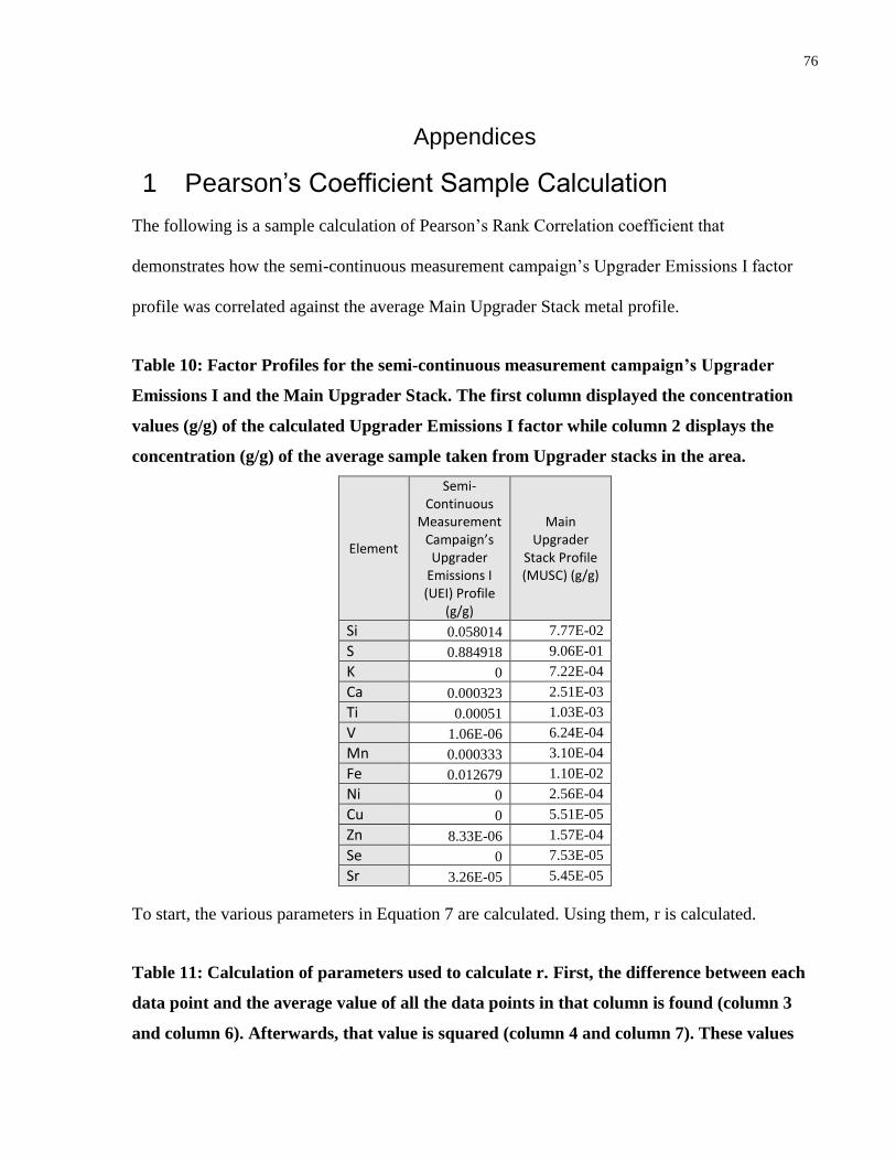
76
Appendices
1 Pearson’s Coefficient Sample Calculation
The following is a sample calculation of Pearson’s Rank Correlation coefficient that
demonstrates how the semi-continuous measurement campaign’s Upgrader Emissions I factor
profile was correlated against the average Main Upgrader Stack metal profile.
Table 10: Factor Profiles for the semi-continuous measurement campaign’s Upgrader
Emissions I and the Main Upgrader Stack. The first column displayed the concentration
values (g/g) of the calculated Upgrader Emissions I factor while column 2 displays the
concentration (g/g) of the average sample taken from Upgrader stacks in the area.
Element
Semi-Continuous
Measurement Campaign’s Upgrader
Emissions I (UEI) Profile
(g/g)
Main Upgrader
Stack Profile (MUSC) (g/g)
Si 0.058014 7.77E-02
S 0.884918 9.06E-01
K 0 7.22E-04
Ca 0.000323 2.51E-03
Ti 0.00051 1.03E-03
V 1.06E-06 6.24E-04
Mn 0.000333 3.10E-04
Fe 0.012679 1.10E-02
Ni 0 2.56E-04
Cu 0 5.51E-05
Zn 8.33E-06 1.57E-04
Se 0 7.53E-05
Sr 3.26E-05 5.45E-05
To start, the various parameters in Equation 7 are calculated. Using them, r is calculated.
Table 11: Calculation of parameters used to calculate r. First, the difference between each
data point and the average value of all the data points in that column is found (column 3
and column 6). Afterwards, that value is squared (column 4 and column 7). These values

77
are added together then their square root is calculated. Finally the values in column 3 and
column 6 are multiplied together (column 8). These values are then added together.
Element UEI
Profile (g/g)
UEI-Ave(UEI) (UEI-
Ave(UEI))2 MUSC (g/g)
MUSC-Ave(MUSC)
(MUSC-Ave(MUSC))2
(UEI-Ave(UEI))*MUSC-
Ave(MUSC)
Si 0.058014 -0.01558746 0.00024297 7.77E-02 0.0007825 6.123E-07 -1.2E-05
S 0.884918 0.811316539 0.65823453 9.06E-01 0.8286223 0.6866149 0.672275
K 0 -0.07360146 0.00541718 7.22E-04 -0.0762011 0.0058066 0.005609
Ca 0.000323 -0.07327846 0.00536973 2.51E-03 -0.0744084 0.0055366 0.005453
Ti 0.00051 -0.07309146 0.00534236 1.03E-03 -0.0758952 0.0057601 0.005547
V 1.06E-06 -0.0736004 0.00541702 6.24E-04 -0.076299 0.0058215 0.005616
Mn 0.000333 -0.07326846 0.00536827 3.10E-04 -0.0766129 0.0058695 0.005613
Fe 0.012679 -0.06092246 0.00371155 1.10E-02 -0.0659709 0.0043522 0.004019
Ni 0 -0.07360146 0.00541718 2.56E-04 -0.0766673 0.0058779 0.005643
Cu 0 -0.07360146 0.00541718 5.51E-05 -0.0768679 0.0059087 0.005658
Zn 8.33E-06 -0.07359313 0.00541595 1.57E-04 -0.0767658 0.005893 0.005649
Se 0 -0.07360146 0.00541718 7.53E-05 -0.0768478 0.0059056 0.005656
Sr 3.26E-05 -0.07356886 0.00541238 5.45E-05 -0.0768686 0.0059088 0.005655
Sum 0.71618345 0.7492559 0.7323803
Square root 0.84627623 0.8655957
From these parameters, r=0.73/(0.85*0.87)=1.