space-time etas models and an improved...
TRANSCRIPT

Space-time ETAS models and an improved extension
Yosihiko Ogata and Jiancang Zhuang
The Institute of Statistical Mathematics, Minami-Azabu 4-6-7, Minato-Ku, Tokyo, 106-8569
Japan, [email protected]
Abstract.
For a sensitive detection of anomalous seismicity such as quiescence and activation in a
region, we need a suitable statistical reference model that represents a normal seismic
activity in the region. Regional occurrence rate of earthquakes is modeled as a function
of previous activity, the specific form of which is based on empirical laws in time and
space such as the modified Omori formula and the Utsu-Seki scaling law of aftershock
area against magnitude, respectively. This manuscript summarizes the development of
the epidemic type aftershock sequence (ETAS) model and proposes an extended version
of the best fitted space-time model that was suggested in Ogata (1998). This model
indicates significantly better fit to seismicity in various regions in and around Japan.
Keywords; aftershock areas, earthquake clusters, ETAS model, modified Omori law,
space-time seismicity model, triggering,
1. Introduction
Seismic quiescence and activation have been attracting attention as the precursors to a large
earthquake, possibly providing useful information on its location, time and/or size (Inouye,
1965; Utsu, 1968; Ohtake et al., 1977; Wyss and Burford, 1987; Kisslinger, 1988;
Keilis-Borok and Malinovskaya, 1964; Sekiya, 1976; Evison, 1977; Sykes and Jaume, 1990).
Ohtake (1980) and Kanamori (1981) reviewed the studies of seismic quiescence, illustrating
gaps in space-time earthquake occurrences, and hypothesizing physical mechanisms. On the
other hand, Lomnitz and Nava (1983) argued that quiescence is merely due to the reduction of
aftershocks of previous large earthquakes. They simulated a space-time cluster process to
illustrate deceptive seismic gaps and quiescences, and claimed that these have little predictive
information about the occurrence time or the magnitude of the next large event.
Thus, it has been difficult to discuss instances of quiescence clearly in the presence of
complex aftershock activity. Also, the quiescence does not always appear clearly, especially
in periods and areas where the activity is high. The appearance of the quiescence also depends
on a threshold magnitude of the earthquakes in the data. Indeed, the recognition of seismic
anomalies seems to be subjective and still seems under development and even controversial.
To overcome these difficulties we first need to use a practical statistical space-time model that
represents the ordinary seismic activity, rather than carrying out a declustering algorithm that
removes aftershock events from a catalog. Using full homogeneous dataset, the successful
model should enable us to detect anomalous temporal deviations of the actual seismicity rate
from that of the modeled occurrence rate. Indeed, the temporal ETAS (Epidemic Type
Aftershock Sequence) model that ignores the spatial factor, has successfully detected quiet

periods relative to the modeled rate by the transformation of occurrence times. (Ogata, 1988,
1989, 1992, 2001; Ogata et al., 2003a).
There are already a number of space-time point-process models that take aftershock clusters
into account (Kagan, 1991; Vere-Jones, 1992; Musmeci and Vere-Jones, 1992; Ogata, 1993,
1998; Rathbun, 1993, 1994; Schoenberg, 1997; Console and Murru, 2001; Zhuang et al.,
2002; and Console et al., 2003). In particular, the epidemic type aftershock sequence model
(ETAS model; Ogata, 1988) is extended by Ogata (1998) to several space-time models that
are constructed based on both empirical studies of spatial aftershock clustering with some
speculative hypotheses. Goodness-of-fit of these are compared to judge the best practical
space-time model among them for the application to both offshore interplate activity and
intraplate activity in inland in and around Japan. The optimal space-time ETAS model is then
extended to the hierarchical Bayesian model (Ogata et al., 2003b; Ogata, 2004). However, the
diagnostic analysis based on the stochastic declustering algorithm reveals a significant bias in
the spatial scaling factor in the model (Zhuang et al., 2004). The purpose of the present paper
is therefore to propose a better fitted model that reduces the bias.
2. Development of the ETAS model.
2.1. Epidemic type aftershock sequence model
The typical aftershock decay is represented by the Modified Omori function,
� (t) = K (t + c) p� , (K, c, p; parameters), (1)
initiated by the main shock at time origin t=0. This formula was proposed by Utsu (1957,
1961) from fits to many datasets as the extension of the Omori law (Omori, 1894). This
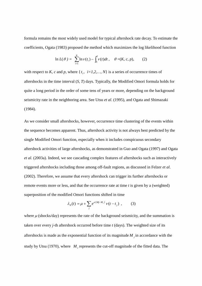
formula remains the most widely used model for typical aftershock rate decay. To estimate the
coefficients, Ogata (1983) proposed the method which maximizes the log likelihood function
ln L(� ) = � ��
�
N
i
T
Si dttt1
)()(ln �� , � =(K, c, p), (2)
with respect to K, c and p, where { ,it i=1,2,…, N} is a series of occurrence times of
aftershocks in the time interval (S, T) days. Typically, the Modified Omori formula holds for
quite a long period in the order of some tens of years or more, depending on the background
seismicity rate in the neighboring area. See Utsu et al. (1995), and Ogata and Shimazaki
(1984).
As we consider small aftershocks, however, occurrence time clustering of the events within
the sequence becomes apparent. Thus, aftershock activity is not always best predicted by the
single Modified Omori function, especially when it includes conspicuous secondary
aftershock activities of large aftershocks, as demonstrated in Guo and Ogata (1997) and Ogata
et al. (2003a). Indeed, we see cascading complex features of aftershocks such as interactively
triggered aftershocks including those among off-fault regions, as discussed in Felzer et al.
(2002). Therefore, we assume that every aftershock can trigger its further aftershocks or
remote events more or less, and that the occurrence rate at time t is given by a (weighted)
superposition of the modified Omori functions shifted in time
,)()( }{� ���
�
jj
MMj ttet c ����
� (3)
where � (shocks/day) represents the rate of the background seismicity, and the summation is
taken over every j-th aftershock occurred before time t (days). The weighted size of its
aftershocks is made as the exponential function of its magnitude jM in accordance with the
study by Utsu (1970), where cM represents the cut-off magnitude of the fitted data. The

coefficient � (magnitude 1� ) measures an efficiency of a shock in generating its aftershock
activity relative to its magnitude. For example, the �-value for Japanese earthquake swarm
activity has been found to scatter in the range [0.35, 0.85], in contrast to non-swarm activity
which is characterized by higher values, namely in [1.2, 3.1] (Ogata, 1992). Note that K
(shocks/day) in the� -function represents the standardized quantity by )}(exp{ ci MM �� ,
which measures the productivity of the aftershock activity during a short period right after the
mainshock (cf. Utsu, 1970; Reasenberg and Jones, 1989). We call the equation (3) the ETAS
(epidemic-type aftershock sequence) model, which was originally proposed for the general
seismic activity in a region (Ogata, 1988, 1992), but also accurately applied to aftershock
sequence itself (Ogata, 1989, 2001; Guo and Ogata, 1997; Ogata et al., 2003a).
For a sequence of the occurrence times associated with magnitudes, we can estimate the
parameters �� ( ,� K, c,� , p) of the ETAS model that are common to all i, by maximizing
the log-likelihood function that is of the same form as the one in equation (2) with the
exception that the Modified Omori intensity function � (t) is replaced by the occurrence
rate )(t�� of ETAS model. See Utsu and Ogata (1997) for computational codes and technical
aspect, and Helmstetter and Sornette (2002), for example, for some discussions of statistical
features of the ETAS model.
2.2. Space-time ETAS model
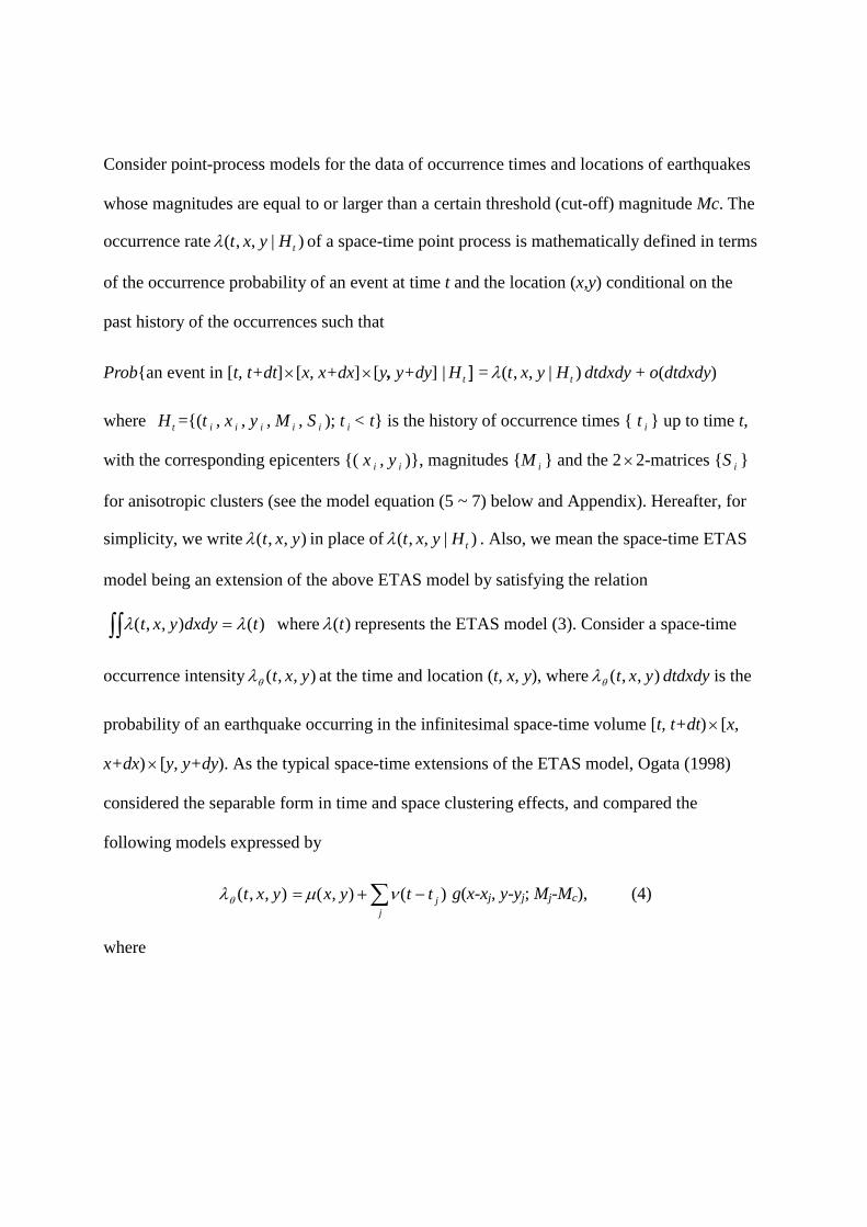
Consider point-process models for the data of occurrence times and locations of earthquakes
whose magnitudes are equal to or larger than a certain threshold (cut-off) magnitude Mc. The
occurrence rate )|,,( tHyxt� of a space-time point process is mathematically defined in terms
of the occurrence probability of an event at time t and the location (x,y) conditional on the
past history of the occurrences such that
Prob{an event in [t, t+dt]� [x, x+dx]� [y, y+dy] | tH ] = )|,,( tHyxt� dtdxdy + o(dtdxdy)
where tH ={(t i , x i , y i , M i , S i ); t i < t} is the history of occurrence times { t i } up to time t,
with the corresponding epicenters {( x i , y i )}, magnitudes {M i } and the 2� 2-matrices {S i }
for anisotropic clusters (see the model equation (5 ~ 7) below and Appendix). Hereafter, for
simplicity, we write ),,( yxt� in place of )|,,( tHyxt� . Also, we mean the space-time ETAS
model being an extension of the above ETAS model by satisfying the relation
�� � )(),,( tdxdyyxt �� where )(t� represents the ETAS model (3). Consider a space-time
occurrence intensity ),,( yxt�
� at the time and location (t, x, y), where ),,( yxt�
� dtdxdy is the
probability of an earthquake occurring in the infinitesimal space-time volume [t, t+dt)� [x,
x+dx)� [y, y+dy). As the typical space-time extensions of the ETAS model, Ogata (1998)
considered the separable form in time and space clustering effects, and compared the
following models expressed by
� ���
jjttyxyxt )(),(),,( ���
�g(x-xj, y-yj; Mj-Mc), (4)
where
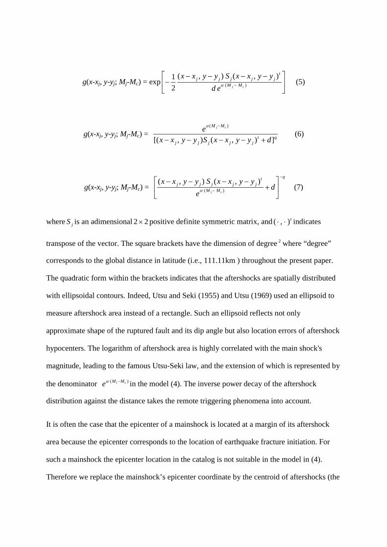
g(x-xj, y-yj; Mj-Mc) = exp ��
���
� �����
� )(
),(),(21
cj MM
tjjjjj
edyyxxSyyxx
� (5)
g(x-xj, y-yj; Mj-Mc) = qtjjjjj
MM
dyyxxSyyxxe cj
]),(),[(
)(
�����
��
(6)
g(x-xj, y-yj; Mj-Mc) = q
MM
tjjjjj d
eyyxxSyyxx
cj
�
���
���
��
����)(
),(),(�
(7)
where jS is an adimensional 22� positive definite symmetric matrix, and t),( �� indicates
transpose of the vector. The square brackets have the dimension of degree 2 where “degree”
corresponds to the global distance in latitude (i.e., 111.11km ) throughout the present paper.
The quadratic form within the brackets indicates that the aftershocks are spatially distributed
with ellipsoidal contours. Indeed, Utsu and Seki (1955) and Utsu (1969) used an ellipsoid to
measure aftershock area instead of a rectangle. Such an ellipsoid reflects not only
approximate shape of the ruptured fault and its dip angle but also location errors of aftershock
hypocenters. The logarithm of aftershock area is highly correlated with the main shock's
magnitude, leading to the famous Utsu-Seki law, and the extension of which is represented by
the denominator )( ci MMe �� in the model (4). The inverse power decay of the aftershock
distribution against the distance takes the remote triggering phenomena into account.
It is often the case that the epicenter of a mainshock is located at a margin of its aftershock
area because the epicenter corresponds to the location of earthquake fracture initiation. For
such a mainshock the epicenter location in the catalog is not suitable in the model in (4).
Therefore we replace the mainshock’s epicenter coordinate by the centroid of aftershocks (the
mean of coordinates of aftershocks) for the model (4). Such centroid of aftershocks could be
closely related to the centroid of the ruptured fault determined in the Harvard CMT catalog
due to Dziewonski et al. (1981). Also, spatial distributions of aftershock epicenters are not
usually isotropic owing to the aforementioned reasons. Appendix summarizes the compiling
procedure for the centroid of clusters and also the matrices jS representing the ellipsoid of
anisotropic clusters. Such a recompiled dataset is useful in the model (4) significantly for
some large earthquakes, whereas, for the remaining supermajority of events, the centroid can
be taken as the epicenter of the original catalog and jS as the identity matrix.
Given the recompiled dataset of origin times and space coordinates of earthquakes together
with their magnitudes and matrices {(t i , x i , y i , M i , jS ); M i �M c , i=1,…,n} during a period
[0,T] and in a region A, we can calculate the log-likelihood function of the parameter ��
( ,� K, c, ,� p,d,q) characterizing the space-time point-process model, which is given by
ln L(� ) = dxdydtyxtyxtN
i
T
S Aiii� � ���
�
1),,(),,(ln
���� . (8)
Interested readers are referred to Daley and Vere-Jones (2002; Section 7) for the derivation of
this formula and Ogata (1998) for the numerical calculations. The maximum likelihood
estimate (MLE) �� ( ,� K , c , ,� p , d , q ) is the one that maximize the function. The
physical dimensions of these parameters are provided in Table 1.
For the comparison of goodness-of-fit of the competing models to a dataset, Akaike’s
Information Criterion (AIC; Akaike, 1974) is useful. The statistic AIC = -2 ln L(� ) +2dim(� )
is computed for each of the models fitted to the data. In comparing models with different
numbers of parameters, addition of the quantity 2 dim(� ), roughly compensates for the
additional flexibility which the extra parameters provide. The model with the lower AIC-value

is taken as giving the better choice for forward prediction purposes. Insofar as it depends on
the likelihood ratio, the AIC can also be used as a rough guide to the model testing. As a rule
of thumb, in testing a model with k+d parameters against a null hypothesis with just k
parameters, we take a difference of 2 in AIC values as a rough estimate of significance at the
5% level.
Ogata (1998) compared the goodness-of-fit of the three cases (5) - (7) of the models for the
following cases where:
C1. homogeneous Poisson field for the background seismicity, ��x ,y��= ��= const., and
isotropic clustering, i.e., Sj = 2x2 identity matrix;
C2. non-homogeneous Poisson field for the background seismicity, ��x ,y���= ����x ,y��where
���x ,y��is a baseline-spline-surface, and isotropic clustering, i.e., Sj = 2x2 identity matrix;
C3. homogeneous Poisson field for the background seismicity, ��x ,y���= ����x ,y��where
���x ,y��is a baseline-spline-surface, and anisotropic clustering, Sj = 2x2 positive-definite
symmetric matrix depending on j (cf., Appendix) and the center of each cluster �xj, yj��is
modified to be the centroid (average) of the coordinates of aftershocks.
According to Ogata (1998) the AIC always chose the model (4) with (7), consequence of
which are as follows:
R1. The triggered clusters in space extend beyond the traditional aftershock regions, showing
a much more diffuse boundary with power law decay rather than a more clearly defined
region with a fairly sharp boundary converging faster than the exponential decay.
R2. There may be perhaps two components (near field and far field) with different
characteristics; the near field component corresponds to the traditional aftershock area

around the ruptured fault, and the far field component may relate to the so called the
'aftershocks in wide sense' such as immigrations of earthquake activity or causal relations
between distant regions, caused by tectonic changes of the stress-field due to the rupture or
dynamic triggering of the seismic waves.
R3. The cluster regions scale with magnitudes firmly owing to the Utsu-Seki formula.
3. Extension of the best fitted space-time model
Using the models (4) with (5) ~ (7), Zhuang et al. (2004) implemented the stochastic
declustering of a data set from Hypocenter Catalog of the Japan Meteorological Agency
(JMA) in order to make diagnostic analysis of space-time features of clusters using the
space-time ETAS models. The majority of the diagnostic results show that the functions for
each component in the formulation of the above best space-time ETAS model (4) with (7)
confirms the superiority to, and shows graphically better fit to various declustered statistics
than the model (4) with (5). Especially, it is shown that the scale of the triggering region is
still an exponential law as formulated in (7). However, one of the important diagnostic
features is that some systematic deviation (bias in slope) is seen from the expected number of
offspring (cf. Figure 2a in the present paper) for the considered data from a central Japan
region that is defined in Section 4. This suggests us that some modification of the model is
desirable.
In Ogata (1998), the common standard form including the models (5) ~ (7) is given by the
multiplication of normalized time and space density distributions besides the multiplication of
size function in such a way that

g(x, y; M) = �(M) ��
���
�
��
��
�
�
�
)(),(),(
)(1
)()1( 1
MyxSyxh
Mctcp t
p
p
���
(9)
where h(x, y) represents the different forms in (5) ~ (7), and the size function is assumed to be
�(M) = const.��(M)� e�M in the paper.
Now, the point of the present extension is to remove the constraint between �(M) and �(M).
This leads to the new model
g(x-xj, y-yj; Mj-Mc) = )()( cj MMe ����
q
MM
tjjjjj d
eyyxxSyyxx
cj
�
���
���
��
����)(
),(),(�
, (10)
which need the eight parameters �� ( ,� K, c, �, �, p, d, q). In the following sections, we
will compare this with the model (4) with (7). Furthermore, from the least square fitting to the
diasgnostic plots, Zhuang et al. (2004) implies that
�~ = 0.50 loge10 � 1.15, (11)
rather than the MLE, � =1.334, in the model (4) with (7) for the central Japan data from the
JMA earthquake catalog. Actually this agrees with the famous empirical formulae log10 A = M
+ 4.0 due to Utsu and Seki (1955), or equivalently log10 L = 0.5M – 1.8 due to Utsu (1961),
where A and L represents the area and length of the aftershock zone, respectively, for the
mainshock magnitude M. Relevantly, the above intersect constants for the land (intraplate)
events are smaller than those for sea (interplate) events, but the slopes 1.0 and 0.5 remain the
same according to Utsu (1969). Related studies on the scaling relations are Shimazaki (1986),
Yamanaka and Shimazaki (1990), and Scholz (1990, Section 4.3.2). Thus, it is also
worthwhile to compare the restricted version of the model (4) with (10) by the fixed value in
(11).

4. Application to the data sets
We use the hypocenter data compiled by the Japan Meteorological Agency (JMA), and
consider three data sets from the areas of tectonically distinctive features and also their
mixture. First data of earthquakes of magnitude (M) 4.5 and larger are chosen from the wide
region 36o ~ 42oN and 141o ~ 145oE (Off the east coast of Tohoku District; see Figures 1) for
all depth down to 100km and for the time span 1926-1995. From now on we refer to this
region as Region A. In Region A the most of large earthquakes took place on the plate
boundary between the North American and subducting Pacific plates. We ignore the depth
axis and consider only two-dimensional locations (longitude and latitude) of earthquakes,
restricting ourselves to the shallow events. Most of the events are distributed within depths
down to sixty kilometers. Another area of interest is the central and western part of Honshu
Island, Japan, the region 34o ~ 38oN and 131o ~ 137oE (referring to Region B) shown in the
Figure 1, where the most earthquakes are considered as intraplate events within the Eurasian
plates. Shallow earthquakes (h�45 km) of M4.0 and larger are considered for the time span
1926 ~ 1995. Finally, we consider the data set of the hypocenter locations of 4586
earthquakes of M5.0 or larger in the region 30o ~ 47oN and 128o ~ 149oE with depths
shallower than 65 km for the period from 1926 through 1995, in and around Japan, referring
to Region C in Figure 1.
The maximum likelihood estimations and AIC comparisons are made for every data set. In
calculating distance between earthquake epicenters, the distance in longitude is reduced to
cos(�y0180o) times as large as that in latitude (one degree corresponds to about 111.11 km),
where y0 is taken to be the latitude of the center of the area. Table 1 lists the estimated
parameters and AICs of respective models when the background intensity is invariant in space
such that �(x,y) = � in (4). The AIC comparison among the considered models shows that the
goodness-of-fit of the models (4) with (7) and (10) are similar performance in the both areas
A and B, but show the better performance of (10) for Region C. However, as discussed in
Ogata (1998), the estimate p� <1 for a long period indicates that the assumption �(x,y) = � in
(4) is inappropriate, which is indeed the common sense among the seismologists.
[Tables 1~3 around here.]
The more realistic versions of the three models are fitted to each data set. Table 2 summarizes
the results for the three models with the location-dependent background intensity (4) with
�(x,y) = ����x,y� where the baseline function ���x,y� is the same ones as represented by the
bi-cubic spline surfaces for the corresponding regions in Ogata (1998). Moreover, we assume
that the matrix Sj is the 2x2 identity one for any event j, meaning the isotropic spatial
clustering. Furthermore, Table 3 summarizes the results for the three models with the
location-dependent background intensity and with anisotropic spatial clustering, where the
matrix Sj for any event j is obtained by the procedure described in Appendix.
The goodness-of-fit of the extended model (4) with (10) become significantly better than the
model with (7) for all the data sets in both Tables 2 and 3. It is noteworthy that each AIC in
Tables 2 and 3 is remarkably smaller than the corresponding AIC in Table 1, although the
justification is not established for the straightforward comparison of AIC of the models with
the adjusted function 0�� (x, y) beforehand and additional explanatory data for the anisotropic
clustering. In fact, the number of coefficients of the B-spline function is 96, 198 and 480 for
the background seismicity ���x,y��of Region A, B and C, respectively, and the AIC
differences confirm the significantly better fit than the homogeneous background seismicity.
The p-values which are smaller than 1.0 in Table 1 now become larger than 1.0, which agrees
with our experience in estimating the ETAS model to various data during a long period of
seismic activity. Therefore, along with the substantial decrease of each AIC in Tables 2 and 3
compared with the AIC of the corresponding models, we believe that the inclusion of the
non-homogeneous background seismicity in the space-time modeling provides the
significantly better performance for the present three data sets. The location-dependent
background intensity model also made the larger estimate value of the coefficient q of the
decay power of distance to the cluster members.
Comparing Tables 2 with 3, we see that the parameter values of the corresponding models are
quite similar and that the decrease of the AIC is not very large in spite of the implicitly used
parameters for the anisotropic clustering. Therefore, it is not very clear whether or not the
anisotropic modeling significantly improves the goodness-of-fit, but the improvement seems
to become clearer as the number of data increases, or threshold magnitude lower. After all,
throughout Tables 1, 2, and 3, it is confirmed that model (4) with (10) for the spatial
clustering improves the goodness-of-fit and its degree of significance depends on the region
of different seismicity patterns. Furthermore, the reducing number of parameter may be
possible by fixing the parameter � in (11) depending on the data, rather than considering the
restriction � = ��in the model (10), which is nothing but the model (7).
5. Diagnostic Analysis by stochastic declustering
4.1 Stochastic declustering
To obtain an objectively declustered catalogue, Zhuang et al. (2002, 2004) proposed the
stochastic declustering method as an alternative to the conventional declustering methods. In
this method, it is not deterministic any more whether an earthquake is a background events or
triggered by another. Instead, each event has a probability to be either a background event or a
direct offspring triggered by others. The main task of the stochastic declustering algorithm is
to estimate this probability for each event according to some models for describing
earthquake clustering features.
The technical key point of the stochastic declustering method is the thinning operation to a
point process (Ogata, 1981, 1998; Daley and Vere-Jones, 2002; Zhuang et al., 2004).
Observing the model (4), the relative contribution of the previous i-th event to the total
conditional intensity at the occurrence time and location of the j-th event, (tj, xj, yj), is
�i,j ���(tj - ti) g(xj-xi, yj-yi; Mi-Mc) / �(tj, xj, yj)
by the definition. That is to say, for each i = 1, 2, …, N, select the j-th event with probability
�i,j, then we can realize a subprocess of the events triggered by the i-th event. In this way, �i,j
can be regarded as the probability of the j-th event being triggered by the i-th event.
Furthermore, the probability of the event j being a background event is �j = (tj, xj, yj) / �(tj, xj,
yj) and the probability that the j-th event is triggered is �j ��� �j = �{i: i<j} �i,j. In other words,
if we select each event j with probabilities �j, we can then form up a new processes being the
background subprocess, with its complement being the clustering subprocess. For the
algorithm of the stochastic declustering, the readers are referred to Zhuang et al. (2002, 2004).
A stochastically declustered catalogue produced from the above procedures is not unique,
because it depends on the random numbers used in the selection of events to form the
background seismicity. Unlike conventional declustering methods, the stochastic declustering
method does not fix the judgement on whether an event is an aftershock or not. Instead, it
gives a probability how each event looks like an aftershock. Namely, the stochastic
declustering is understood to be a simulation, or precisely bootstrap resampling, and we
understand this to be an advantage because it shows the uncertainty about earthquake activity.
Thus, simply by using random simulation of the thinning method, we can easily produce
stochastic copies of declustered catalogue. Stochastic declustering realizes (simulates) many
possible configurations of background events depending on the seeds of random number so
that we could make use of graphical statistics based on the repeated thinning realizations to
discuss uncertainty and significance of an interesting phenomena as the conventional
bootstrapping does.
4.2. Distribution of distance to offspring events relative to ancestor’s magnitude
In order to examine the appropriateness of the function form exp{�(M -Mc)}/d in the model
(7), Zhuang et al. (2004) calculated the distance ri,j between a triggered event j and its direct
ancestor, event i, that belong to a given magnitude band (Mi�) M using the set of clusters
that are declustered from the coordinates data of 8283 target events of M4.2 or larger from the
rectangular region 130o - 146oE and 33o - 42.5oN (see Region D in Figure 1) in the depth
range (0, 100) km during the period from 10,001-th day from 1926 up until the end of 1999.
Then, to estimate the scaling parameter d in (7) for each magnitude band M instead of
maximizing the log-likelihood function to possibly many resampled data due to the stochastic
declustering, Zhuang et al. (2004) considers maximizing the log-pseudo-likelihood
log L(D) = ��� };{ MMi i ��
���
��
���
�
�
�
qji
jiq
jijji Dr
rDq)(
)1(2log 2
,
,1
};{,� .
Figure 2a shows the plot of D against the magnitude band �M=(M-0.05, M+0.05) for the
model (7) that is the similar to Figure 14 in Zhuang et al. (2004). The plots should correspond
to )(ˆˆ cMMaed � where d and � are the MLE of the model (4) with (7). However, the D plot
alignment has significantly biased smaller slope than that of the log-plot of )(ˆˆ cMMaed � as seen
in Figure 2a. On the other hand, Figure 2c shows the similar plot by the application of the
presently proposed model (10), which has little systematic deviation. The significance and
stability of the plots are demonstrated in Figures 2b and 2d by the corresponding simulated
dataset by respective model.
6. Concluding remarks
The detected rate of earthquakes in a catalog generally changes not only with location, but
also with time, due to the configulation of seismometers and changing observational
environments in space and time. Therefore, we have studied the seismicity using data of the
lowest threshold magnitude above which earthquakes are completely detected. The estimated
parameter values themselves depend by scale difference on the magnitude thresholds of
complete detection, except for the �, �, p and q-values, in principle. However, the proportion
of earthquakes smaller than the minimum threshold magnitude for the complete data is
usually substantial because the number of earthquakes increase exponentially
(Gutenberg-Richter’s law) if all of earthquakes were completely detected. From the viewpoint
of effective use of data, this is quite wasteful in the statistical analysis of seismic activity.
Thus, our next step for the practical space-time seismicity analysis is to develop the presently
improved model taking account of the space-time detection rate as a function of magnitude,
time and location as implemented in Ogata and Katsura (1993) for space-time changes of
b-value in the Gutenberg-Richter magnitude-frequency law.
Appendix: Data Processing for Anisotropic Clusters
We have proposed the model (4) with (10) as the extended version of the model (4) with (7)
that was best fitted in Ogata (1998). This model shows significantly better fit to seismicity in
a wide region. The difference of the goodness-of-fit depends on the region of the analysis.
Thus, we calculate the maximum likelihood estimates (MLE) of the space-time ETAS model,
which show regional characteristics of seismicity such as the background seismicity,
aftershock population sizes, aftershock productivity, aftershock decay rate, scaling of spatial
clustering, etc., throughout the considered period.
In order to replace the epicenter coordinate ),( jj yx in the catalog by the centroid of
aftershock locations for the coordinate ),( jj yx in the model (4), we estimate retrospectively
using the aftershock distribution as follows. First, we identify clusters of aftershocks, i
=1,2,…, N j , by the algorithm that is provided below. Then, we take the average ),( yx of
the locations of the cluster members to replace the epicenter of the main shock ),( jj yx only
when the difference is significant as determined by the statistical procedure (Ogata, 1998).
Also, the anisotropic spatial aftershock distribution represented by the matrix jS in (4) for an
ellipsoid is estimated as follows. We fit a bi-variate normal distribution to the location
coordinates of the aftershocks in each cluster (see below) to obtain the maximum likelihood
estimate of the average vector ( 21 ˆ,ˆ �� ) and the covariance matrix with the adimensional
elements 21 ˆ,ˆ �� and � for jS in (4) in the form
�S ���
����
�2221
2121
����
����.
This is listed in the recompiled catalog only when they are significantly different from the
identity matrix as the null hypothesis (i.e., 121 ���� and 0�� ). Specifically, according to
Ogata (1998), the minimum AIC procedure (Akaike, 1974), instead of the likelihood ratio test,
is adopted among all the nested models which include the null hypothesis. For the rest of
events in the cluster, the null hypothesis is always adopted; namely, the same coordinate as
the epicenter given in the catalog and the identity matrix for jS .
The algorithm for identifying the aftershock clusters starts with selecting the largest shock in
the original catalog for the mainshock. If there are plural largest shocks, the earliest one is
adopted for the main shock. Then, to form a cluster, we set a space-time window with the
bounds of distance and time depending on the magnitude of the main shock, based on the
empirical laws of aftershocks (c.f., Utsu, 1969). For example, the algorithm in Ogata et al.
(1995), except for foreshocks, describes its explicit form. The identification of the aftershock
cluster is surely subjective to some degree in spite of the method based on the empirical laws.
Nevertheless, this is useful for our eventual objective to estimate the centroidal coordinates
and coefficients for the anisotropy of the clusters for some large earthquakes. Indeed, we can
apply a simple similar compiling procedure based on the aftershocks during only a few days’
period. Also, the stochastic declustering algorithm will be useful.
Acknowledgements
This research is partly supported by Grant-in-Aid 14380128 for Scientific Research (B2), The
Ministry of Education, Culture, Sport, Science and Technology. Furthermore, J.Z. is also
supported by a post-doctoral program P04039 funded by the Japan Society for the Promotion
of Science.
References
Akaike, H., 1974. A new look at the statistical model identification, IEEE Trans. Automat. Control, AC-19:
716-723.
Console, R. and Murru, M., 2001. A simple and testable model for earthquake clustering, J. Geophys. Res.,
106: 8699-8711.
Console, R., Murru, M. and Lombardi, A.M., 2003. Refining earthquake clustering models, J. Geophys.
Res., 108: 2468, 10.1029/2002JB002130.
Daley, D.J. and Vere-Jones, D., 2002. An Introduction to the Theory of Point Processes, Volume 1, second
edition, Springer-Verlag, New York.
Dziewonski, A.M., Chou, T.A. and Woodhouse, J.H., 1981. Determination of earthquake source
parameters from waveform data for studies of global and regional seismicity, J. Geophys. Res., 86:
2825-2852.
Evison, F.F., 1977. The precursory earthquake swarm, Phys. Earth Planet. Inter. 15: 19-23.
Felzer, K.R., Becker, T.W., Abercrombie, R.E., Ekstrom, G. and Rice, J.R., 2002. Triggering of the 1999
Mw7.1 Hector Mine earthquake by aftershocks of the 1992 Mw7.3 Landers earthquake, J. Geophys. Res.,
107: 2190, doi: 10.1029/ 2001JB000911.
Guo, Z. and Ogata, Y., 1997. Statistical relations between the parameters of aftershocks in time, space and
magnitude, J. Geophys. Res., 102: 2857-2873.
Helmstetter, A. and Sornette, D., 2002. Subcritical and supercritical regimes in epidemic models of
earthquake aftershocks, J. Geophys. Res., 107: 2237, doi: 10.1029/ 2001JB001580.
Inouye, W., 1965. On the seismicity in the epicentral region and its neighborhood before the Niigata
earthquake (in Japanese), Kenshin-jiho (Quarterly J. Seismol.) 29: 139-144.
Kagan, Y.Y., 1991. Likelihood analysis of earthquake catalogues, J. Geophys. Res., 106: 135-148.
Kanamori, H., 1981. The nature of seismicity patterns before large earthquakes, in Earthquake Prediction,
Maurice Ewing Series, 4, D. Simpson and P. Richards, Editors, Am. Geophys. Union, Washington D.C.:
1-19.
Keilis-Borok, V.I. and Malinovskaya, L.N., 1964. One regularity in the occurrence of strong earthquakes, J.
Geophys. Res., 70: 3019-3024.
Kisslinger, C., 1988. An experiment in earthquake prediction and the 7th May 1986 Andreanof Islands
Earthquake, Bull. Seismol. Soc. Am., 78: 218-229.
Lomnitz, C. and Nava, F.A., 1983. The predictive value of seismic gaps, Bull. Seismol. Soc. Amer., 73:
1815-1824.

Musmeci, F. and Vere-Jones, D., 1992. A space-time clustering model for historical earthquakes, Ann. Inst.
Statist. Math., 44: 1-11.
Omori, F., 1894. On the aftershocks of earthquakes, J. Coll. Sci. Imp. Univ. Tokyo, 7: 111-200.
Ogata, Y., 1981. On Lewis' simulation method for point processes, IEEE Transactions on Information
Theory, IT-27: 23-31.
Ogata, Y., 1983. Estimation of the parameters in the modified Omori formula for aftershock frequencies by
the maximum likelihood procedure, J. Phys. Earth, 31: 115-124.
Ogata, Y., 1988. Statistical models for earthquake occurrences and residual analysis for point processes, J.
Amer. Statist. Assoc., 83: 9-27.
Ogata, Y., 1989. Statistical model for standard seismicity and detection of anomalies by residual analysis,
Tectonophysics, 169: 159-174.
Ogata, Y., 1992. Detection of precursory seismic quiescence before major earthquakes through a statistical
model, J. Geophys. Res., 97: 19845-19871.
Ogata, Y., 1993. Space-time modelling of earthquake occurrences, Bull. Int. Statist. Inst., 55, Book 2:
249-250.
Ogata, Y., 1998. Space-time point-process models for earthquake occurrences, Ann. Inst. Statist. Math., 50:
379-402.
Ogata, Y., 2001. Increased probability of large earthquakes near aftershock regions with relative quiescence,
J. Geophys. Res., 106: 8729-8744.
Ogata, Y., 2004. Space-time model for regional seismicity and detection of crustal stress changes, J.
Geophys. Res., 109, B3, B03308, doi:10.1029/ 2003JB002621.
Ogata, Y. and Abe, K., 1989. Some statistical features of the long term variation of the global and regional
seismic activity. Int. Statist. Rev., 59: 139-161.
Ogata, Y., and Shimazaki, K., 1984. Transition from aftershock to normal activity: the 1965 Rat Islands
earthquake aftershock sequence, Bull. Seismol. Soc. Am., 74: 1757-1765.
Ogata, Y. and Katsura, K. 1993. Analysis of temporal and spatial heterogeneity of magnitude frequency
distribution inferred from earthquake catalogues, Geophys. J. Int., 113: 727-738.
Ogata, Y., T. Utsu, and K. Katsura, 1995. Statistical features of foreshocks in comparison with other
earthquake clusters, Geophys. J. Int., 121: 233-254.
Ogata, Y., Jones, L.M. and Toda, S., 2003a. When and where the aftershock activity was depressed:
Contrasting decay patterns of the proximate large earthquakes in southern California, J. Geophys. Res.,
108: 2318, 10.1029/2002JB002009.
Ogata, Y., Katsura, K. and Tanemura, M., 2003b. Modelling of heterogeneous space-time seismic activity
and its residual analysis, Appl. Statist., 52: 499-509.
Ohtake, M., 1980. Earthquake prediction based on the seismic gap with special reference to the 1978
Oaxaca, Mexico earthquake (in Japanese), Report of the National Research Center for Disaster Prevention,
23: 65-110.
Ohtake, M., T. Matumoto, and G.V. Latham, 1977. Seismicity gap near Oaxaca, southern Mexico as a
probable precursor to a large earthquake, Pure Apple. Geophys., 115: 375-385.
Rathbun S.L., 1993. Modeling marked spatio-temporal point patterns, Bull. Int. Statist. Inst., 55, Book 2:
379-396.
Rathbun S.L., 1994. Asymptotic properties of the maximum likelihood estimator for spatio-temporal point
processes, in special issue on Spatial Statistic of J. Statist. Plann. Inf., 51: 55-74.
Reasenberg, P.A. and Jones, L.M., 1994. Earthquake aftershocks: update, Science, 265, 1251-1252.
Schoenberg, R.P., 1997. Assessment of Multi-dimensional Point Processes, Ph.D. Thesis, University of
California, Berkeley.
Scholz, C.H., 1990. The Mechanics of Earthquakes and Faulting, Cambridge University Press, Cambridge,
UK., 439pp.
Sekiya, H., 1976. The seismicity preceding earthquakes and its significance in earthquake prediction (in
Japanese), Zisin II (J. Seismol. Soc. Japan), 29: 299-312.
Shimazaki, K., 1986. Small and large earthquakes: The effects of thickness of seismogenetic layer and the
free surface, in Earthquake Source Mechanics, AGU Geophys. Mono. 37, ed. S. Das, J. Boatwright, and C.
Scholz, Washington D.C.: American Geophysical Union: 119-144.
Sykes, L.R. and Jaume, S.C., 1990. Seismic Activity on Neighboring faults as a Long-term Precursor to
Large Earthquakes in the San Francisco Bay Area, Nature, 348: 595-599.
Utsu, T., 1957. Magnitude of earthquakes and occurrence of their aftershocks (in Japanese), Zisin II (J.
Seismol. Soc. Japan): 10, 35-45.
Utsu, T., 1961. Statistical study on the occurrence of aftershocks, Geophys. Mag., 30: 521-605.

Utsu, T., 1968. Seismic activity in Hokkaido and its vicinity (in Japanese), Geophys. Bull. Hokkaido Univ.,
13: 99-103.
Utsu, T., 1969. Aftershocks and earthquake statistics (I): some parameters which characterize an aftershock
sequence and their interrelations, J. Faculty Sci., Hokkaido Univ., Ser. VII (geophysics) 3: 129-195.
Utsu, T., 1970. Aftershocks and earthquake statistics (II): Further investigation of aftershocks and other
earthquake sequences based on a new classification of earthquake sequences, J. Faculty Sci., Hokkaido
Univ., Ser. VII (geophysics), 3: 198-266.
Utsu, T. and Seki, A., 1955. Relation between the area of aftershock region and the energy of the main
shock (in Japanese), Zisin (J. Seismol. Soc. Japan), 2nd Ser., ii, 7: 233-240.
Utsu, T., Ogata, Y. and Matsu'ura, R.S., 1995. The centenary of the Omori formula for a decay law of
aftershock activity. J. Phys. Earth, 43: 1-33.
Wyss, M. and Burford, R.O., 1987. Occurrence of a predicted earthquake on the San Andreas fault, Nature,
329: 323-325.
Utsu, T. and Ogata, Y., 1997. Statistical Analysis of Seismicity (SASeis) for Seismicity, IASPEI Software
Library, 6, International Association of Seismology and Physics of the Earth's Interior: 13-94.
Vere-Jones, D., 1992. Statistical methods for the description and display of earthquake catalogues, in
Statistics in the Environmental and Earth Sciences (eds. A. Walden, and P. Guttorp), Edward Arnold,
London: 220-236.
Yamanaka, Y. and Shimazaki, K., 1990. Scaling relationship between the number of after-shocks and the
size of the main shock, J. Phys. Earth, 38, 305-324.
Zhuang, J., Ogata, Y. and Vere-Jones, D., 2002. Stochastic declustering of space-time earthquake
occurrences, J. Amer. Statist. Assoc., 97: 369-380.
Zhuang, J., Ogata, Y. and Vere-Jones, D., 2004. Analyzing earthquake clustering features by using
stochastic reconstruction, J. Geophys. Res.,109, B5: B05301, 10.1029/2003JB002879.

Figure captions
Fig. 1. Epicenter of the earthquakes of magnitude 4.0 and larger (depth�100 km) in and
around Japan for the period 1926-1995, and regions A, B, C, and D from which the
space-time models are applied.
Fig. 2. Circles indicate the mode of distance-distribution (i.e., D ; the most frequently
appeared distance from the parent to the cluster members, cf. Section 4.2) against the
corresponding magnitudes of triggering (parent) earthquakes calculated based on the
stochastically declustered clusters that are reconstructed from the JMA data from Region D:
the panels (a) and (c) show those where the stochastic-declustering algorithm is performed
using the model (7) and (10), respectively; and the panels (b) and (d) are the same plots for a
simulated data using the model (7) and (10), respectively. The solid straight lines in (a, b) and
dotted lines in (c, d) indicate the function )(ˆˆ cMMaed � of magnitude M with the maximum
likelihood estimate of the corresponding model, respectively; while the straight lines in (c)
and (d) indicate the function )(ˆˆ cMMed �� .

Table 1. The MLEs of space-time ETAS model fitted to the three datasets 1926-1995.
Model �� K c � � p d q AIC
unit events/day/degree 2 days magnitude 1� degrees 2
Off the east coast of Tohoku District (Region A) M�4.5, 4333 events
(7) .707� 10-3 .967� 10-4 .836� 10-2 1.281 1.281 0.909 .184� 10-2 1.565 0.0
(10) .711� 10-3 .988� 10-4 .840� 10-2 1.962 1.326 0.910 .203� 10-2 1.570 0.6
(11) .708� 10-3 .106� 10-3 .842� 10-1 1.273 (1.15) 0.910 .222� 10-2 1.571 -0.6*
Central and western Honshu (Region B) M�4.0, 3007 events
(7) .335� 10-3 .167� 10-3 .514� 10-2 0.910 0.910 0.961 .341� 10-3 1.405 0.0
(10) .337� 10-3 .171� 10-4 .520� 10-2 0.935 0.740 0.961 .403� 10-3 1.408 -3.2*
(11) .330� 10-3 .148� 10-3 .512� 10-2 0.972 (1.15) 0.960 .261� 10-3 1.397 19.0
All Japan data (Region C) M�5.0, 4586 events
(7) .985� 10-5 .274� 10-3 .740� 10-2 1.113 1.113 0.910 .434� 10-2 1.513 0.0
(10) .101� 10-4 .290� 10-3 .748� 10-2 1.154 0.891 0.911 .552� 10-2 1.524 -13.2*
(11) .101� 10-4 .247� 10-3 .745� 10-2 1.626 (1.15) 0.910 .413� 10-2 1.515 -0.7
For each dataset the AIC-values are the relative value of the model (7) for an easier
comparison. The original AIC values of the model (7) are AICA=32897.4, AICB=15836.7 and
AICC=45161.4 for the dataset from regions A, B, and C, respectively, which are the same
values given in Ogata (1998). * indicates the smallest AIC value among the models (7), (10)
and (11).
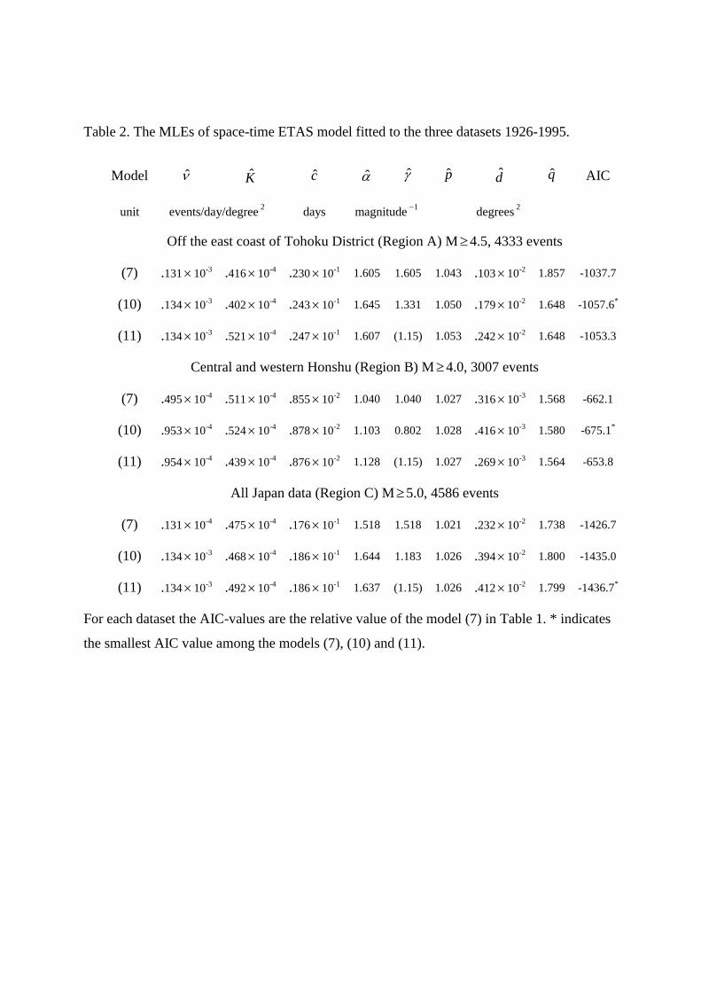
Table 2. The MLEs of space-time ETAS model fitted to the three datasets 1926-1995.
Model � K c � � p d q AIC
unit events/day/degree 2 days magnitude 1� degrees 2
Off the east coast of Tohoku District (Region A) M�4.5, 4333 events
(7) .131� 10-3 .416� 10-4 .230� 10-1 1.605 1.605 1.043 .103� 10-2 1.857 -1037.7
(10) .134� 10-3 .402� 10-4 .243� 10-1 1.645 1.331 1.050 .179� 10-2 1.648 -1057.6*
(11) .134� 10-3 .521� 10-4 .247� 10-1 1.607 (1.15) 1.053 .242� 10-2 1.648 -1053.3
Central and western Honshu (Region B) M�4.0, 3007 events
(7) .495� 10-4 .511� 10-4 .855� 10-2 1.040 1.040 1.027 .316� 10-3 1.568 -662.1
(10) .953� 10-4 .524� 10-4 .878� 10-2 1.103 0.802 1.028 .416� 10-3 1.580 -675.1*
(11) .954� 10-4 .439� 10-4 .876� 10-2 1.128 (1.15) 1.027 .269� 10-3 1.564 -653.8
All Japan data (Region C) M�5.0, 4586 events
(7) .131� 10-4 .475� 10-4 .176� 10-1 1.518 1.518 1.021 .232� 10-2 1.738 -1426.7
(10) .134� 10-3 .468� 10-4 .186� 10-1 1.644 1.183 1.026 .394� 10-2 1.800 -1435.0
(11) .134� 10-3 .492� 10-4 .186� 10-1 1.637 (1.15) 1.026 .412� 10-2 1.799 -1436.7*
For each dataset the AIC-values are the relative value of the model (7) in Table 1. * indicates
the smallest AIC value among the models (7), (10) and (11).

Table 3. The MLEs of space-time ETAS model fitted to the three datasets 1926-1995.
Model � K c � � p d q AIC
unit events/day/degree 2 days magnitude 1� degrees 2
Off the east coast of Tohoku District (Region A) M�4.5, 4333 events
(7) .131� 10-3 .382� 10-4 .231� 10-1 1.612 1.612 1.043 .102� 10-2 1.600 -1059.3
(10) .134� 10-3 .375� 10-4 .245� 10-1 1.657 1.326 1.050 .182� 10-2 1.662 -1081.4*
(11) .135� 10-3 .491� 10-4 .248� 10-1 1.617 (1.15) 1.043 .102� 10-2 1.600 -1077.6
Central and western Honshu (Region B) M�4.0, 3007 events
(7) .946� 10-4 .477� 10-4 .866� 10-2 1.057 1.057 1.027 .316� 10-3 1.577 -678.6
(10) .954� 10-4 .489� 10-4 .895� 10-2 1.126 0.804 1.029 .423� 10-3 1.589 -693.8*
(11) .955� 10-4 .406� 10-4 .890� 10-2 1.148 (1.15) 1.028 .274� 10-3 1.575 -672.3
All Japan data (Region C) M�5.0, 4586 events
(7) .131� 10-3 .412� 10-4 .176� 10-1 1.549 1.549 1.020 .221� 10-2 1.752 -1453.6
(10) .135� 10-3 .398� 10-4 .186� 10-1 1.484 1.196 1.026 .396� 10-2 1.828 -1521.1
(11) .135� 10-3 .428� 10-4 .186� 10-1 1.673 (1.15) 1.026 .423� 10-2 1.826 -1522.5*
For each dataset the AIC-values are the relative value of the model (7) in Table 1. * indicates
the smallest AIC value among the models (7), (10) and (11).