span-restorable mesh network design (1) w. d. grover trlabs & university of alberta © wayne d....
Post on 21-Dec-2015
214 views
TRANSCRIPT
Span-restorable Mesh Span-restorable Mesh NetworkNetwork
Design (1)Design (1)W. D. Grover
TRLabs & University of Alberta© Wayne D. Grover 2002, 2003
E E 681 - Module 11
( Version for book website Dec. 2003)
E E 681 - Module 11 © Wayne D. Grover 2002, 2003 2
Concepts to be covered
• Basics of Mesh-restorable networks
• The concept of span restoration
• The lower-bound on redundancy in mesh restorable network
• Three basic approaches for mesh Spare Capacity Placement (SCP) Design
- Sakauchi “cut oriented” formulation
- Herzberg “arc-path” formulation
- “Transportation-like” problem formulation (to be covered in next lecture)
E E 681 - Module 11 © Wayne D. Grover 2002, 2003 3
• (1) many real networks are highly mesh-like in their topology
• (2) for restoration, generalized re-routing over the graph can permit greater sharing of spare capacity
– the redundancy will go down in proportion to the average nodal degree
• (3) the network can be its own computer for the real-time solution of the restoration re-routing problem
– the network can self-organize restoration pathsets is a split-second
– without any external control or databases
• (4) if a network is mesh-oriented it is more flexible and adaptable to unforeseen patterns of demand
– the network can continually self-organize its mapping of physical transmission to logical transport configuration to suit time-and-spatially varying demandpatterns
Key ideas and vision behind “mesh” restoration
E E 681 - Module 11 © Wayne D. Grover 2002, 2003 4
TORINO
GENOVA
ALESSANDRIA
PISA
MILANOBRESCIA
SAVONA
BOLOGNA
VERONA
VICENZA
VENEZIA
FIRENZEANCONA
PESCARA
PIACENZA
MILANO2
PERUGIA
L’AQUILA
ROMA
ROMA2
NAPOLI SALERNO
CATANZARO
POTENZA
BARI
TARANTO
CAGLIARI
SASSARI
FOGGIA
PALERMOMESSINA
REGGIO C.
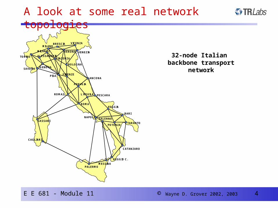
32-node Italian backbone transport
network
A look at some real network topologies
E E 681 - Module 11 © Wayne D. Grover 2002, 2003 5
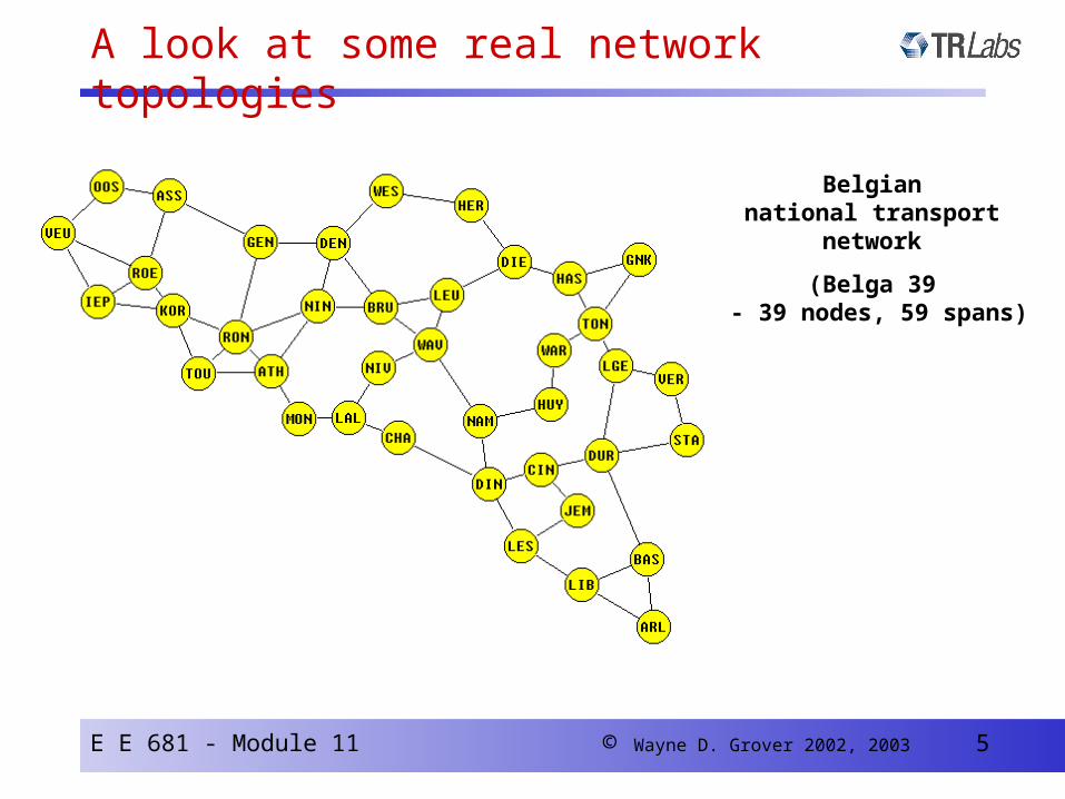
Belgiannational transport
network
(Belga 39 - 39 nodes, 59 spans)
A look at some real network topologies
E E 681 - Module 11 © Wayne D. Grover 2002, 2003 6
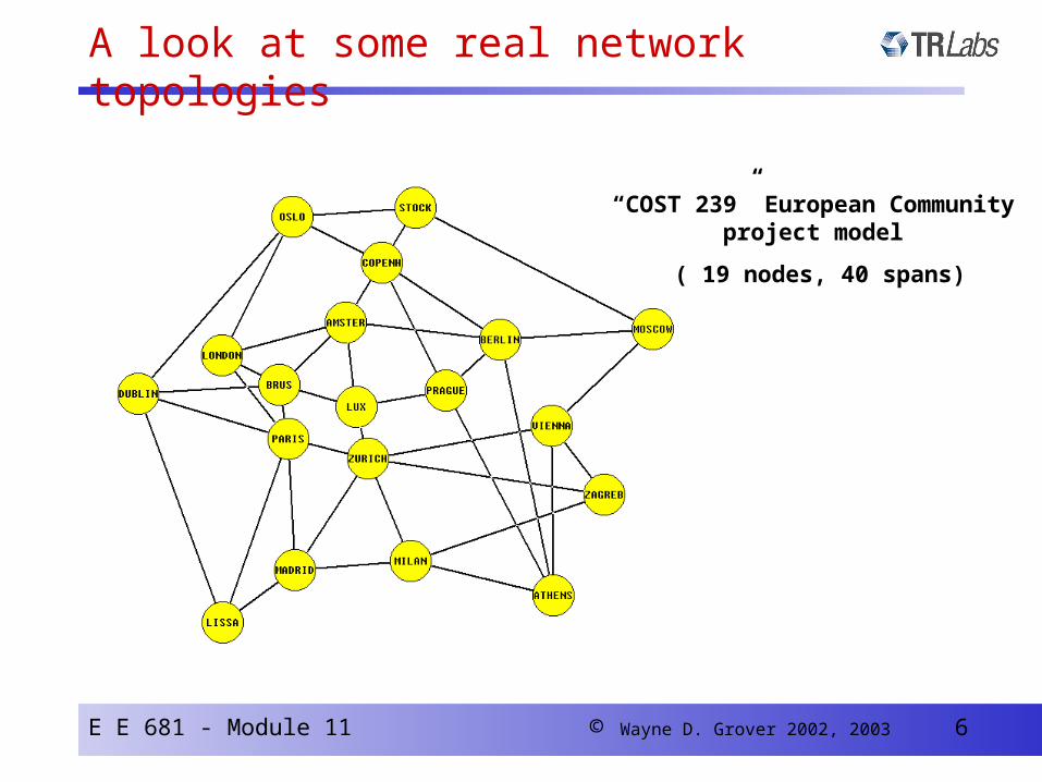
“COST 239” European Communityproject model
( 19 nodes, 40 spans)
A look at some real network topologies
E E 681 - Module 11 © Wayne D. Grover 2002, 2003 7
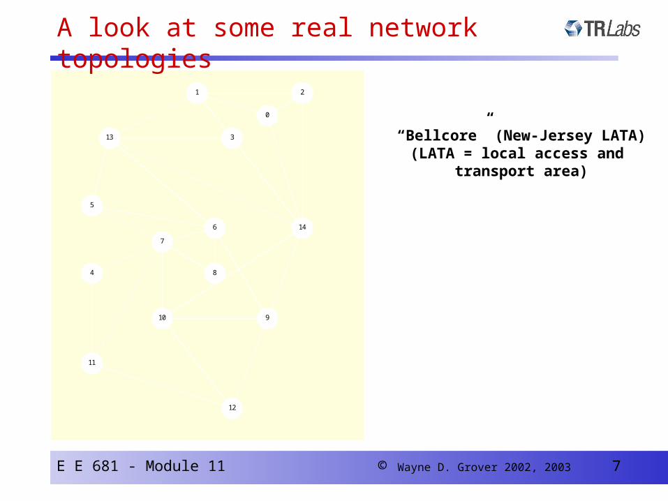
“Bellcore” (New-Jersey LATA)(LATA = local access and
transport area)
0
1 2
3
4
5
6
7
8
910
11
12
13
14
A look at some real network topologies
E E 681 - Module 11 © Wayne D. Grover 2002, 2003 8
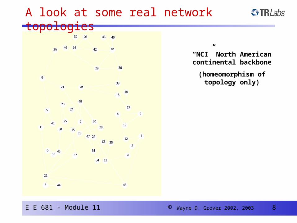
“MCI” North Americancontinental backbone
(homeomorphism oftopology only)
0
1
2
345
6
7
8
9
10
11
12
13
14
15
16
17
18
19
2021
22
23
24
25
26
27
28
29
30
31
32
33
34
35
36
37
38
39
40
41
42
43
44
45
46
47
48
49
50
5152
A look at some real network topologies
E E 681 - Module 11 © Wayne D. Grover 2002, 2003 9
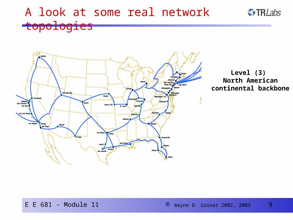
Level (3) North American
continental backbone
A look at some real network topologies
E E 681 - Module 11 © Wayne D. Grover 2002, 2003 10
Basics of Mesh-restorable networks
(28 nodes, 31 spans)
30% restoration70% restoration100% restoration
span cut
E E 681 - Module 11 © Wayne D. Grover 2002, 2003 11
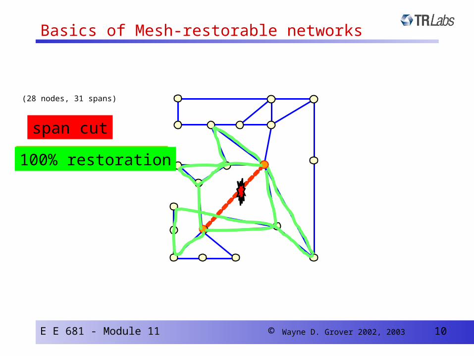
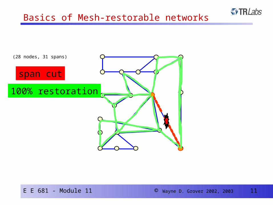
Basics of Mesh-restorable networks
(28 nodes, 31 spans)
span cut
40% restoration70% restoration100% restoration
E E 681 - Module 11 © Wayne D. Grover 2002, 2003 12
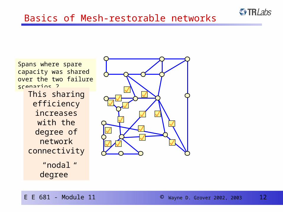
Basics of Mesh-restorable networks
Spans where spare capacity was shared over the two failurescenarios ? .....
This sharing efficiency
increases with the degree of
network connectivity
“nodal degree”
E E 681 - Module 11 © Wayne D. Grover 2002, 2003 13
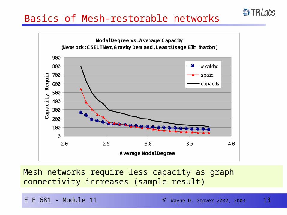
Basics of Mesh-restorable networks
Nodal Degree vs. Average Capacity(Network: CSELTNet, Gravity Demand, Least Usage Elimination)
0
100
200
300
400
500
600
700
800
900
2.0 2.5 3.0 3.5 4.0
Average Nodal Degree
Cap
acit
y R
equ
ired
w orking
spare
capacity
Mesh networks require less capacity as graph connectivity increases (sample result)
E E 681 - Module 11 © Wayne D. Grover 2002, 2003 14
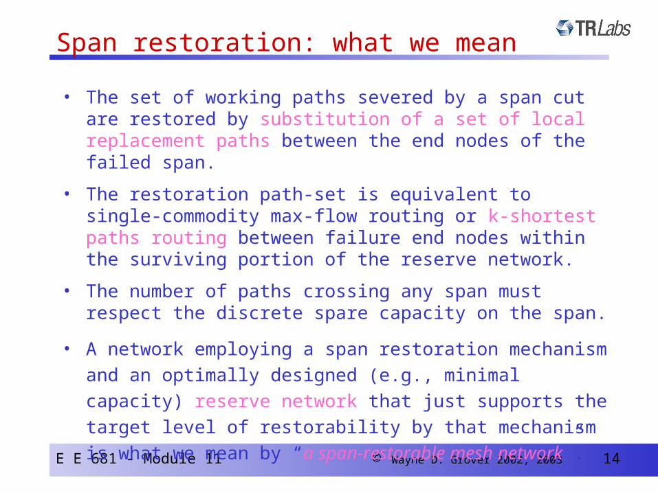
Span restoration: what we mean
• The set of working paths severed by a span cut are restored by substitution of a set of local replacement paths between the end nodes of the failed span.
• The restoration path-set is equivalent to single-commodity max-flow routing or k-shortest paths routing between failure end nodes within the surviving portion of the reserve network.
• The number of paths crossing any span must respect the discrete spare capacity on the span.
• A network employing a span restoration mechanism and an
optimally designed (e.g., minimal capacity) reserve network that
just supports the target level of restorability by that mechanism is
what we mean by “a span-restorable mesh network”.
E E 681 - Module 11 © Wayne D. Grover 2002, 2003 15
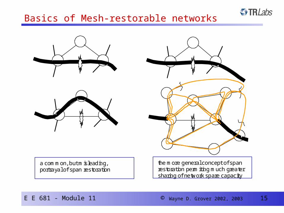
Basics of Mesh-restorable networks
a common, but misleading, portrayal of span restoration
the more general concept of span restoration permiting much greater sharing of network spare capacity
E E 681 - Module 11 © Wayne D. Grover 2002, 2003 16
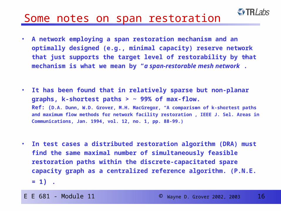
• A network employing a span restoration mechanism and an optimally
designed (e.g., minimal capacity) reserve network that just supports the
target level of restorability by that mechanism is what we mean by “a span-
restorable mesh network”.
• It has been found that in relatively sparse but non-planar graphs, k-shortest
paths > ~ 99% of max-flow.Ref: (D.A. Dunn, W.D. Grover, M.H. MacGregor, “A comparison of k-shortest paths and maximum flow
methods for network facility restoration”, IEEE J. Sel. Areas in Communications, Jan. 1994, vol. 12, no.
1, pp. 88-99.)
• In test cases a distributed restoration algorithm (DRA) must find the same
maximal number of simultaneously feasible restoration paths within the
discrete-capacitated spare capacity graph as a centralized reference
algorithm. (P.N.E. = 1) .
Some notes on span restoration
E E 681 - Module 11 © Wayne D. Grover 2002, 2003 17
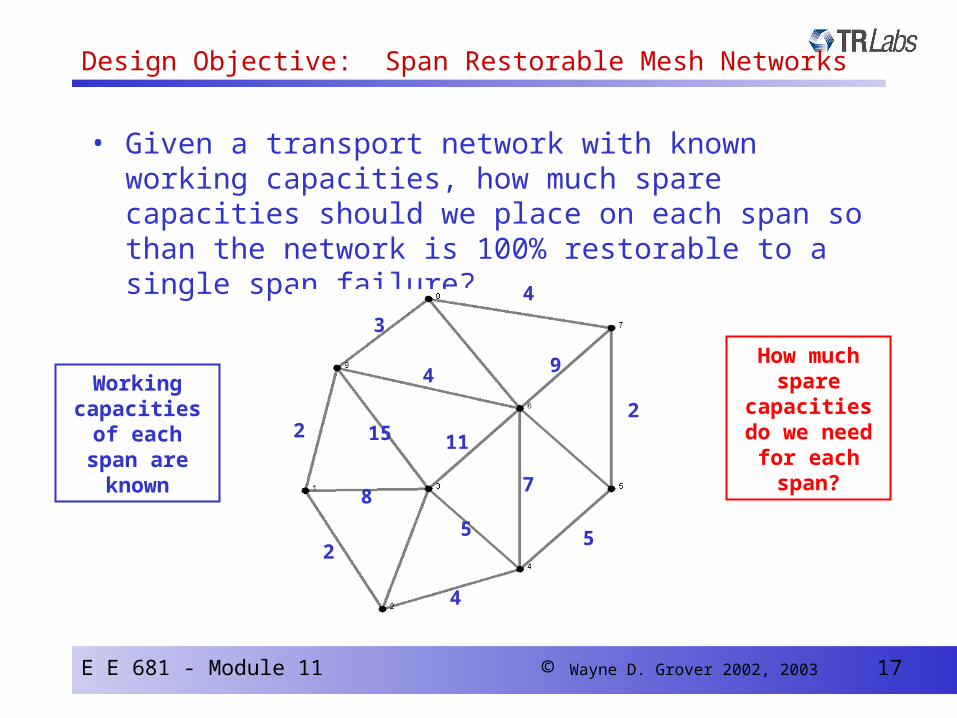
Design Objective: Span Restorable Mesh Networks
• Given a transport network with known working capacities, how much spare capacities should we place on each span so than the network is 100% restorable to a single span failure?
Working capacities
of each span are known
How much spare
capacities do we need
for each span?
4
2
5
3
11
9
15
4
4
2
25
78
E E 681 - Module 11 © Wayne D. Grover 2002, 2003 18
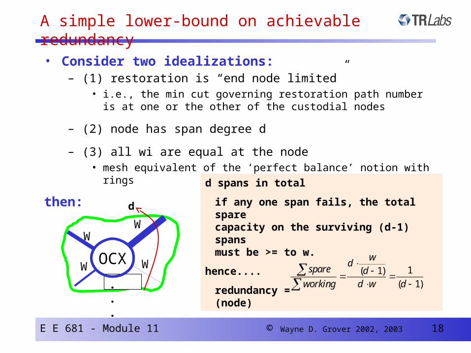
• Consider two idealizations:– (1) restoration is “end node limited”
• i.e., the min cut governing restoration path number is at one or the other of the custodial nodes
– (2) node has span degree d
– (3) all wi are equal at the node • mesh equivalent of the ‘perfect balance’ notion with rings
then:
. . .
OCX
W
WW
W
d spans in total
if any one span fails, the total sparecapacity on the surviving (d-1) spansmust be >= to w.
hence....
redundancy =(node)
1( 1)( 1)
wd
spare dworking d w d
d
A simple lower-bound on achievable redundancy
E E 681 - Module 11 © Wayne D. Grover 2002, 2003 19
A simple lower-bound on achievable redundancy
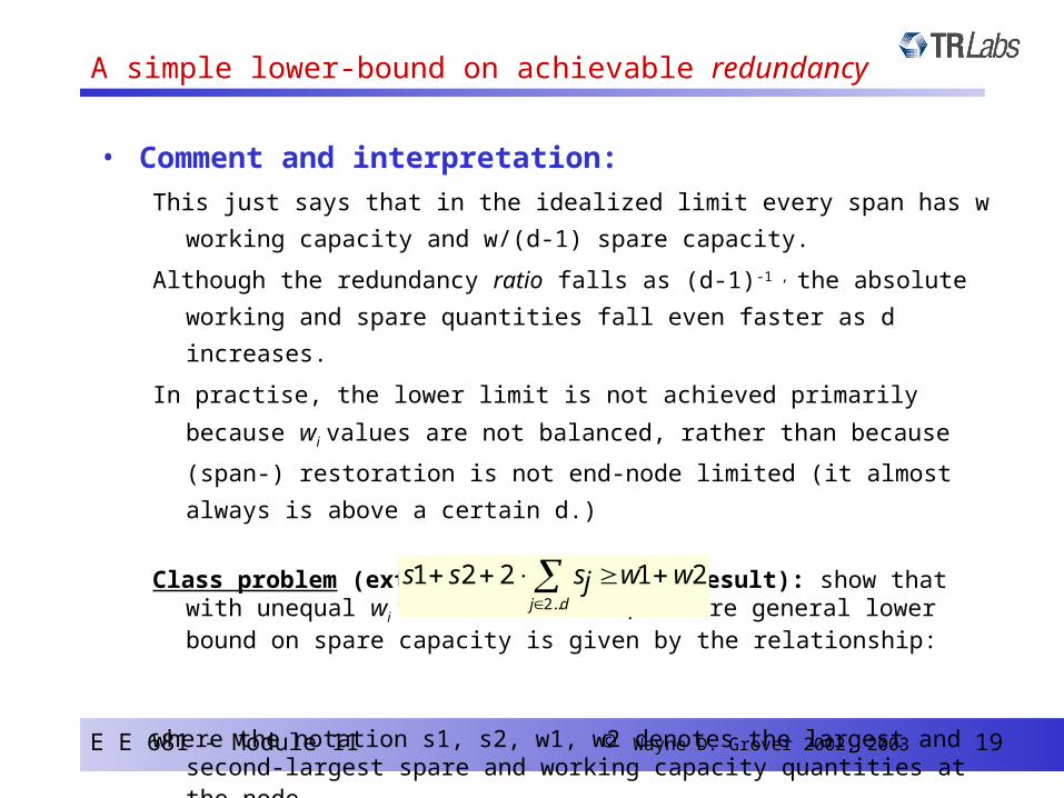
• Comment and interpretation:
This just says that in the idealized limit every span has w working capacity and
w/(d-1) spare capacity.
Although the redundancy ratio falls as (d-1)-1 , the absolute working and spare
quantities fall even faster as d increases.
In practise, the lower limit is not achieved primarily because wi values are not
balanced, rather than because (span-) restoration is not end-node limited (it
almost always is above a certain d.)
Class problem (extension of the basic result): show that with unequal wi values at a node, a more general lower bound on spare capacity is given by the relationship:
where the notation s1, s2, w1, w2 denotes the largest and second-largest spare and working capacity quantities at the node.
2..
1 2 2 1 2j d
s s s w wj
Overview of three basic Overview of three basic approaches for mesh spare approaches for mesh spare
capacity designcapacity design
• Sakauchi - “cut oriented” formulation
• Herzberg - “arc - path” formulation
• “Transportation-like” problem formulation
Note: In these methods, the working paths are first shortest-path routed before solving the spare capacity placement problem. This is what we later refer to as the “non-joint” problem.

E E 681 - Module 11 © Wayne D. Grover 2002, 2003 21
Where:
S = set of all spans
ci = cost of a spare link on span i.
si = number of spare links assigned to span i.
Ci = set of “partial cutsets” relevant to restoration of span i.
= 1 if span j is a member of the cth partial cutset relevant to restoration of span i , 0 otherwise.
c = an individual cutset in the set Ci
wi = the number of working links on span i (working demands are routed prior to solving for the spare capacity.)
jc
(Ref: H. Sakauchi, et al., “A self-healing network with an economical spare-channel assignment”, IEEE GLOBECOM ‘90, pp. 438-443, 1990.)
mini
c sii
S
{ }j i
j s wc j is
;c C i Si S.t.
Sakauchi’s “min-cut max-flow” approach for spare capacity design
E E 681 - Module 11 © Wayne D. Grover 2002, 2003 22
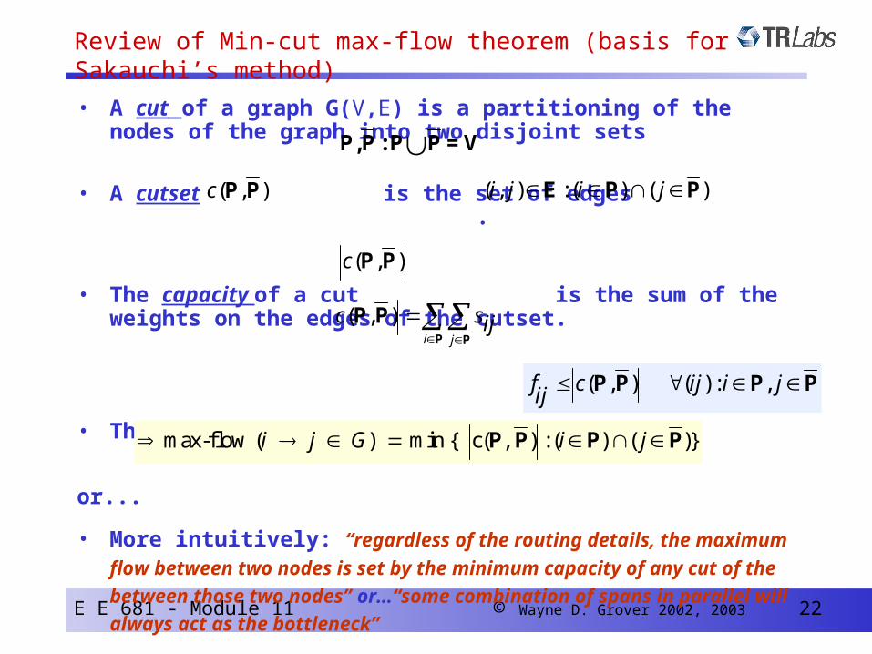
• A cut of a graph G(V,E) is a partitioning of the nodes of the graph into two disjoint sets
• A cutset is the set of edges .
• The capacity of a cut is the sum of the weights on the edges of the cutset.
• The min-cut max-flow theorem is that :
or...
• More intuitively: “regardless of the routing details, the maximum flow
between two nodes is set by the minimum capacity of any cut of the
between those two nodes” or…“some combination of spans in parallel will
always act as the bottleneck”
P,P : P P = V( , ) : ( ) ( )i j i j E P P
max-flow ( ) min { c( , ) : ( ) ( )}i j G i j P P P P
( , )i j
c sij
P P
P P
( , ) ( ) : ,f c ij i jij
P P P P
( , )c P P
( , )c P P
Review of Min-cut max-flow theorem (basis for Sakauchi’s method)
E E 681 - Module 11 © Wayne D. Grover 2002, 2003 23
A
B
E
C
D
F
20
620
68
6
6
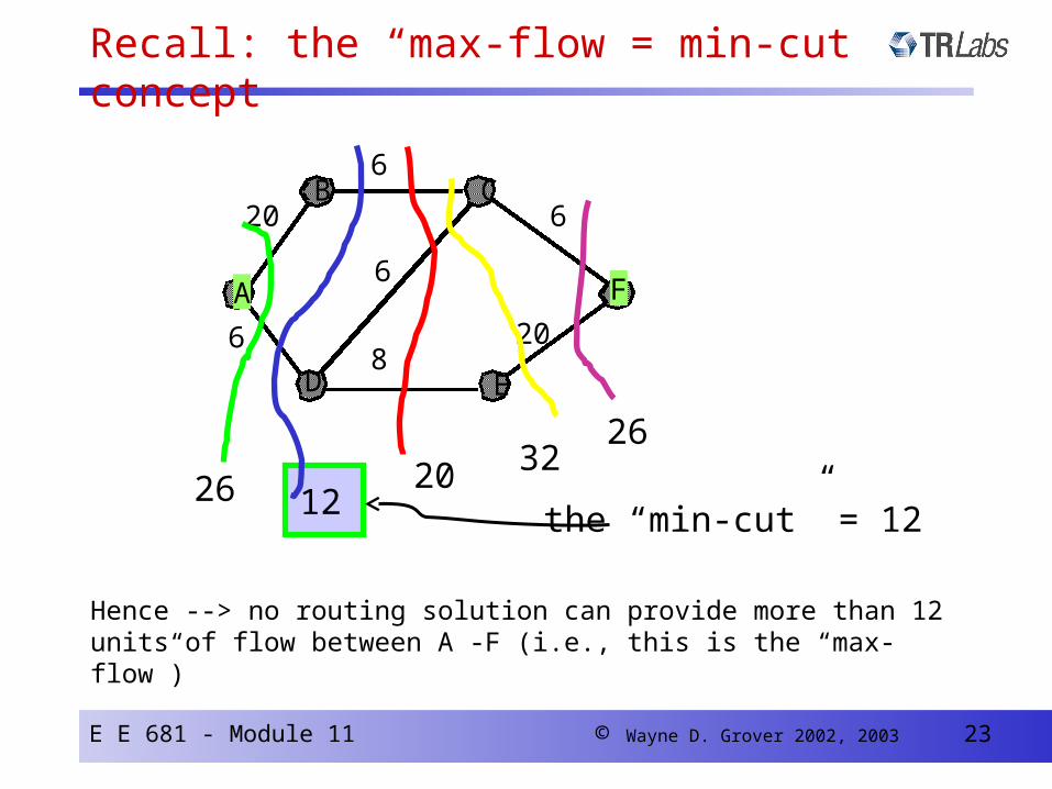
26 1220 32
26
the “min-cut” = 12
Hence --> no routing solution can provide more than 12 units of flow between A -F (i.e., this is the “max-flow”)
Recall: the “max-flow = min-cut” concept
E E 681 - Module 11 © Wayne D. Grover 2002, 2003 24
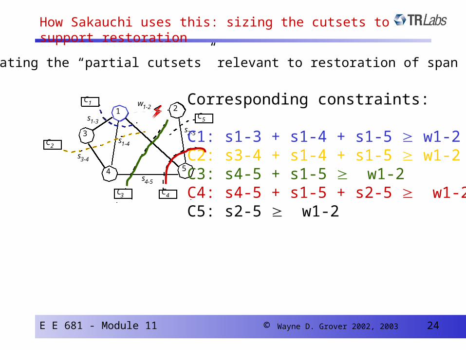
1 2
4
3
5
w1-2
s1-4
s3-4
s1-3
s2-5
s4-5
C1
C2
C3 C4
C5
Illustrating the “partial cutsets” relevant to restoration of span (1-2):
Corresponding constraints:
C1: s1-3 + s1-4 + s1-5 w1-2C2: s3-4 + s1-4 + s1-5 w1-2C3: s4-5 + s1-5 w1-2C4: s4-5 + s1-5 + s2-5 w1-2C5: s2-5 w1-2
How Sakauchi uses this: sizing the cutsets to support restoration
E E 681 - Module 11 © Wayne D. Grover 2002, 2003 25
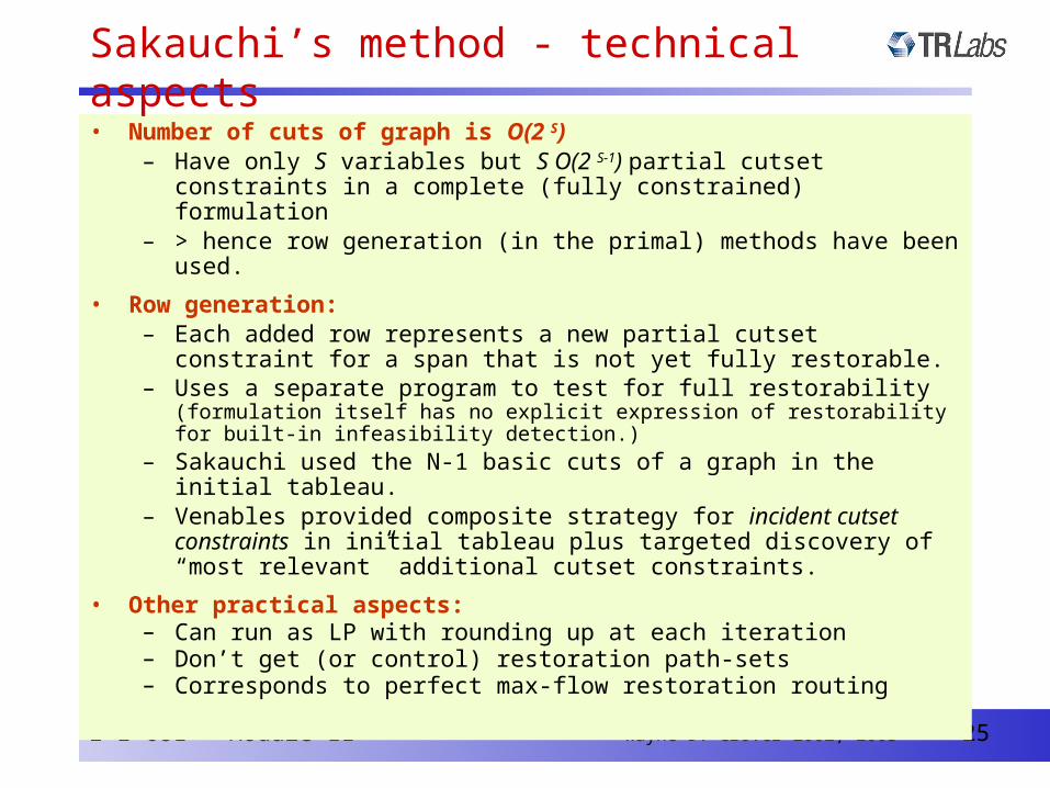
• Number of cuts of graph is O(2 S)– Have only S variables but S O(2 S-1) partial cutset constraints in a complete
(fully constrained) formulation– > hence row generation (in the primal) methods have been used.
• Row generation:– Each added row represents a new partial cutset constraint for a span that is
not yet fully restorable.– Uses a separate program to test for full restorability (formulation itself has no
explicit expression of restorability for built-in infeasibility detection.)– Sakauchi used the N-1 basic cuts of a graph in the initial tableau.– Venables provided composite strategy for incident cutset constraints in
initial tableau plus targeted discovery of “most relevant” additional cutset constraints.
• Other practical aspects:– Can run as LP with rounding up at each iteration– Don’t get (or control) restoration path-sets– Corresponds to perfect max-flow restoration routing
Sakauchi’s method - technical aspects
E E 681 - Module 11 © Wayne D. Grover 2002, 2003 26
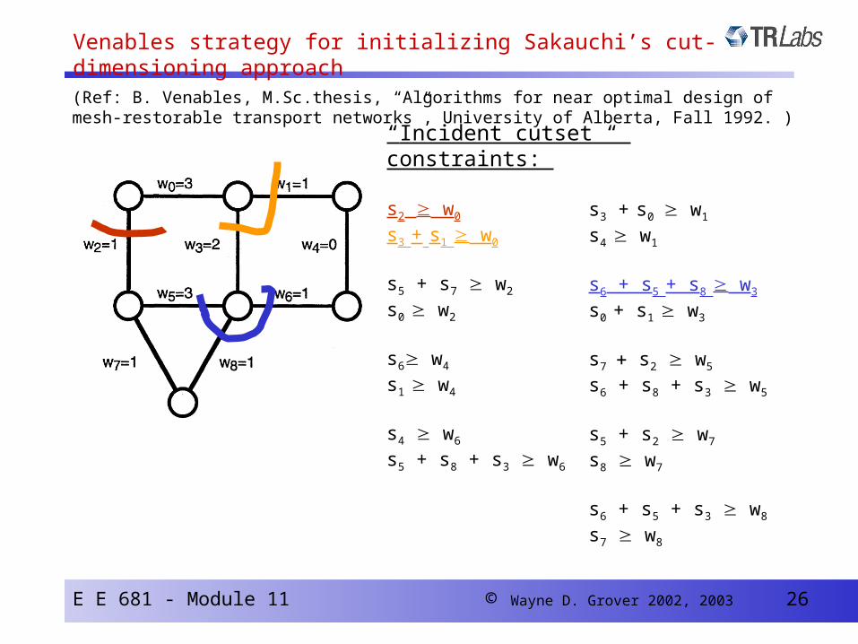
“Incident cutset “ constraints:
s2 w0
s3 + s1 w0
s5 + s7 w2
s0 w2
s6 w4
s1 w4
s4 w6
s5 + s8 + s3 w6
s3 + s0 w1
s4 w1
s6 + s5 + s8 w3
s0 + s1 w3
s7 s2 w5
s6 + s8 + s3 w5
s5 + s2 w7
s8 w7
s6 + s5 + s3 w8
s7 w8
(Ref: B. Venables, M.Sc.thesis, “Algorithms for near optimal design of mesh-restorable transport networks”, University of Alberta, Fall 1992. )
Venables strategy for initializing Sakauchi’s cut- dimensioning approach
E E 681 - Module 11 © Wayne D. Grover 2002, 2003 27
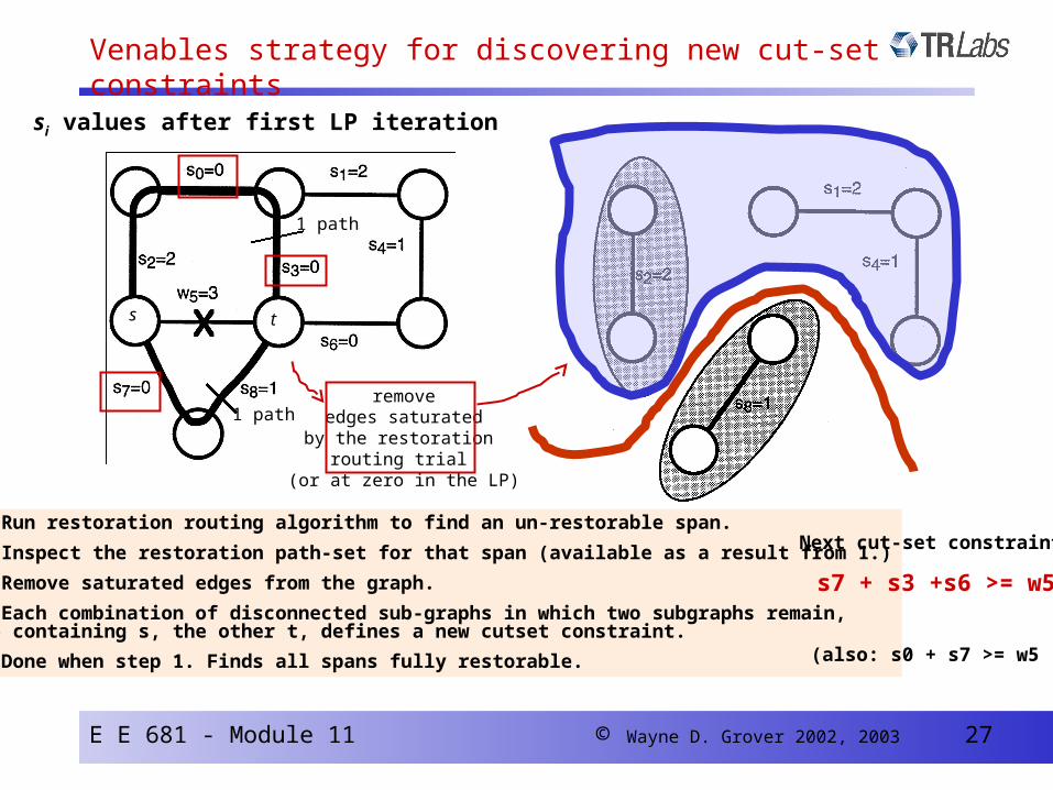
1. Run restoration routing algorithm to find an un-restorable span.
2. Inspect the restoration path-set for that span (available as a result from 1.)
3. Remove saturated edges from the graph.
4. Each combination of disconnected sub-graphs in which two subgraphs remain, one containing s, the other t, defines a new cutset constraint.
5. Done when step 1. Finds all spans fully restorable.
Next cut-set constraint:
s7 + s3 +s6 >= w5
(also: s0 + s7 >= w5 )
s t
remove edges saturated by the restoration
routing trial (or at zero in the LP)
1 path
1 path
si values after first LP iteration
Venables strategy for discovering new cut-set constraints
E E 681 - Module 11 © Wayne D. Grover 2002, 2003 28
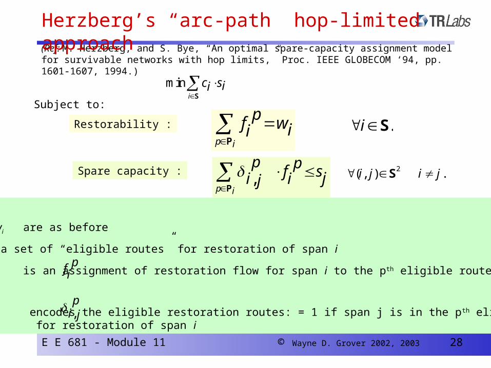
Where:
• S, ci, si, wi are as before
• Pi is a set of “eligible routes” for restoration of span i
• is an assignment of restoration flow for span i to the pth eligible route
• encodes the eligible restoration routes: = 1 if span j is in the p th eligible route for restoration of span i
,pi j
pfi
mini
c sii
S
2( , ) .i j i j S
p i
pf wii
P
.i S
,p i
p pf sji ij
P
Subject to:
Restorability :
Spare capacity :
(Ref: M. Herzberg, and S. Bye, “An optimal spare-capacity assignment model for survivable networks with hop limits,” Proc. IEEE GLOBECOM ‘94, pp. 1601-1607, 1994.)
Herzberg’s “arc-path” hop-limited approach
E E 681 - Module 11 © Wayne D. Grover 2002, 2003 29
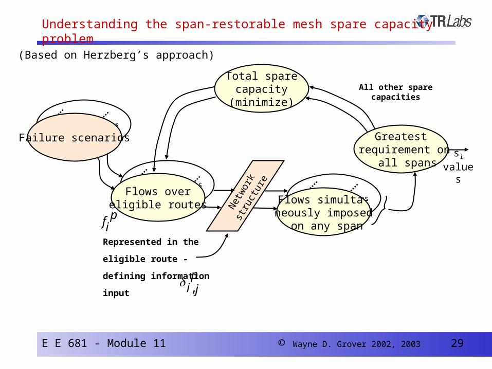
Understanding the span-restorable mesh spare capacity problem
Net
wor
k st
ruct
ure
Failure scenarios
Failure scenarios
Failure scenarios
Greatest requirement on
all spans
Total sparecapacity
(minimize)
Failure scenarios
Flows overeligible routes Flows simulta-
neously imposed on any span
All other spare capacities
si values
(Based on Herzberg’s approach)
pfi
Represented in the
eligible route - defining
information input ,pi j

E E 681 - Module 11 © Wayne D. Grover 2002, 2003 30
Solving Herzberg’s SCP ...
Input Parameters to Solvers
Output (Variables) from Solvers
Working capacities of each span i
Set of eligible restorationroutes for each span failure i
wi
Pi, i,j p
Unit cost for each span i c i
Spare capacities of each span i
Restoration Flow p
s i
f i p
Restoration routes finder for all network spans
Shortest path routing
LPsolve
LPsolve
E E 681 - Module 11 © Wayne D. Grover 2002, 2003 31
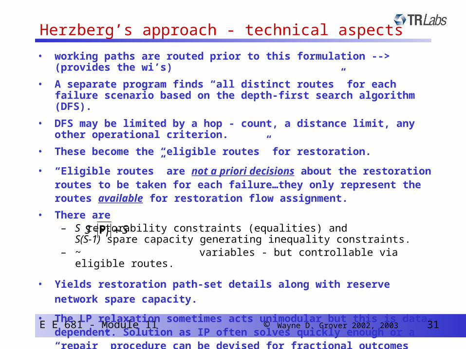
• working paths are routed prior to this formulation --> (provides the wi’s)
• A separate program finds “all distinct routes” for each failure scenario based on the depth-first search algorithm (DFS).
• DFS may be limited by a hop - count, a distance limit, any other operational criterion.
• These become the “eligible routes” for restoration.
• “Eligible routes” are not a priori decisions about the restoration routes to be taken for each failure…they only represent the routes available for restoration flow assignment.
• There are– S restorability constraints (equalities) and
S(S-1) spare capacity generating inequality constraints. – ~ variables - but controllable via eligible routes.
• Yields restoration path-set details along with reserve network spare capacity.
• The LP relaxation sometimes acts unimodular but this is data-dependent. Solution as IP often solves quickly enough or a “repair” procedure can be devised for fractional outcomes when solved as LP.
S Si P
Herzberg’s approach - technical aspects
E E 681 - Module 11 © Wayne D. Grover 2002, 2003 32
500
550
600
650
700
750
800
850
900
2 3 4 5 6 7 8 9
Design Hop Limit, H
To
tal
Sp
are
Cap
acit
y
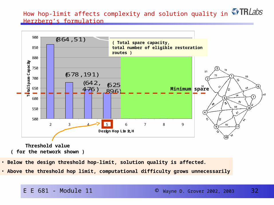
(864, 51)
(678, 191)
(625, 1351)
(625, 1687)
(642, 476)
(625, 896)
Threshold value( for the network shown )
( Total spare capacity, total number of eligible restoration routes )
Minimum spare
• Below the design threshold hop-limit, solution quality is affected.
• Above the threshold hop limit, computational difficulty grows unnecessarily
How hop-limit affects complexity and solution quality in Herzberg’s formulation

E E 681 - Module 11 © Wayne D. Grover 2002, 2003 33
• In practice,
– hop limits can easily be converted to mileage limits or combined hop / distance limits in generating the eligible route-sets for the formulation.
– the basic idea of a single network-wide hop limit can evolves into approaches such as adapting hop limits per span (and per working route in the joint formulations) so as to assure a minimum representation of route diversity, within a computational “budget” for numbers of variables and constraints.
Some practical notes re: “hop limit” concept