SPE 112873

Efficient Ensemble-Based Closed-Loop Production Optimization

Yan Chen, Dean S. Oliver, SPE, University of Oklahoma and Dongxiao Zhang, SPE, University of Southern California

Copyright 2008, Society of Petroleum Engineers

This paper was prepared for presentation at the 2008 SPE Improved Oil Recovery Symposium held in Tulsa, Oklahoma, U.S.A., 19-23 April 2008.

This paper was selected for presentation by an SPE program committee following review of information contained in an abstract submitted by the author(s).Contents of the paper have not been reviewed by the Society of Petroleum Engineers and are subject to correction by the author(s). The material does notnecessarily reflect any position of the Society of Petroleum Engineers, its officers, or members. Electronic reproduction, distribution, or storage of any part of thispaper without the written consent of the Society of Petroleum Engineers is prohibited. Permission to reproduce in print is restricted to an abstract of not morethan 300 words; illustrations may not be copied. The abstract must contain conspicuous acknowledgment of SPE copyright.

AbstractWith the advances in smart well technology, substantially higher oil recovery can be achieved by intelligentlymanaging the operations in a closed-loop optimization framework. The closed-loop optimization consists of twoparts: geological model updating and production optimization. Both of these parts require gradient information tominimize or maximize an objective function: squared data mismatch or the net present value (or other quantitiesdepending on financial goals), respectively. Alternatively, an ensemble-based method can acquire the gradientinformation through the correlations provided by the ensemble. Computation of the optimal controls in this way isnearly independent of the number of control variables, reservoir simulator and simulation solver. In this paper, wepropose an ensemble-based closed-loop optimization method that combines a novel ensemble-based optimizationscheme (EnOpt) with the ensemble Kalman filter (EnKF). The EnKF has recently been found suitable for sequentialdata assimilation in large-scale nonlinear dynamics. It adjusts reservoir model variables to honor observations andpropagates uncertainty in time. The EnOpt optimizes the expectation of the net present value based on the updatedreservoir models. The proposed method is fairly robust, completely adjoint-free and can be readily used with anyreservoir simulator. The ensemble-based closed-loop optimization method is illustrated with a waterflood examplesubject to uncertain reservoir description. Results are compared with other possible reservoir operation scenarios,such as, wells with no controls, reactive control, and optimization with known geology. The comparison shows thatthe ensemble-based closed-loop optimization is able to history match the main geological features and increase thenet present value to a level comparable with the hypothetical case of optimizing based on known geology.

IntroductionProduction optimization offers the potential to substantially increase ultimate oil recovery by developing an im-proved operating plan for a particular reservoir of interest. Since the economic objective involves evaluations offuture achievements, it requires a reservoir simulation model for prediction and is usually referred to as a model-based optimization technique. Due to limited access to the reservoir, the reservoir geological model is subject tohigh uncertainty. In order to obtain a suitable production strategy for the reservoir of interest, production opti-mization needs to be combined with a parameter estimation method that reduces the uncertainty of the estimateof the reservoir geological properties. Closed-loop optimization (Brouwer et al., 2004; Sarma et al., 2005b; Wanget al., 2007) combines production optimization with data assimilation to form a real time reservoir management.Data assimilation is a sequential model updating method, where the estimate of the uncertain parameters is up-dated continuously to be consistent with the production data available in time. The workflow of the closed-loopoptimization technique is typically as follows (see Fig. 1). An initial geological model is built using available priorknowledge of the reservoir and the initial production strategy is chosen based on this prior knowledge. At timeswhen production data are available, the reservoir geological model is updated, and the updated geological modelprovides the basis for a better estimate of the true reservoir behavior. The production strategy is then optimizedbased on the newly updated reservoir model. This process can be carried out in real time, and the management ofthe reservoir is kept up-to-date.

Both model updating and production optimization are optimization problems. Model updating aims at mini-mizing the mismatch between the model predictions and the historical production data. It is commonly known as

2 SPE 112873

Figure 1: The flowchart for closed-loop optimization.

history matching in petroleum reservoir applications. Production optimization aims at maximizing the net presentvalue (NPV) or other quantities depending on financial goals. Gradient-based approaches are commonly usedto solve optimization problems. Since multiphase flow and transport problems are nonlinear, the gradient-basedmethod is usually carried out in an iterative form. A series of linearizations (iterations) are performed in the searchfor a minimum, and at each iteration a gradient is needed to determine the search direction. Various gradientcalculation methods including numerical perturbation, sensitivity equation and adjoint method have been devel-oped. The numerical perturbation method (finite difference approximation) is straightforward to implement butthe computation involved is proportional to the number of unknown parameters. The number of unknown param-eters of the geological model is usually large, two or more parameters per gridblock, although for some problems itmay be possible to reduce the number of parameters describing important aspects of the model (Van Doren et al.,2008). For the production optimization, controls of wells (well constraints) are the unknowns and the number ofcontrol variables is proportional to the number of wells and the number of times at which the control variablesare changed. The numerical perturbation method becomes extremely expensive when the number of unknownparameters is large. Computation of gradients from the adjoint method is independent of the number of unknowns,but requires access to the simulator source code and substantial code development. Li et al. (2003) pointed outthat the coefficient matrix of the adjoint equations is simply the transpose of the Jacobian matrix used in a fullyimplicit reservoir simulator. By extracting and saving the Jacobian matrices, the process of deriving individualadjoint equation can be avoided. Sarma et al. (2005a) used similar idea and developed a modified adjoint methodfor production optimization. But the use of this modified optimization method requires a fully implicit reservoirsimulator, a specific form of the objective function and considerable data storage.

Alternatively, an ensemble-based method can be used to compute an approximation to the gradient through thesensitivity provided by the ensemble, and the simulator only serves as a black box. Approximating the sensitivityfrom the ensemble gives us great flexibility of using different reservoir simulators and simulation solvers. Sensitivitycan be easily computed by processing the inputs and outputs of all the ensemble runs and the computational costis nearly independent of the number of unknown parameters. One of the ensemble-based methods, the ensembleKalman filter (EnKF), has attracted great research interests since the original work of Evensen (1994). The EnKFhas been found suitable for sequential data assimilation in large-scale nonlinear dynamics (Houtekamer and Mitchell,2001; Mitchell et al., 2002; Bertino et al., 2003). Specifically, it has been shown to be suitable for history matchingproblem with possible modifications (Nævdal et al., 2005; Gu and Oliver, 2005; Liu and Oliver, 2005; Haugen et al.,2006; Chen et al., 2007; Li and Reynolds, 2007; Gu and Oliver, 2007). The EnKF utilizes the ensemble-basedsensitivity to adjust an ensemble of geological models to be consistent with the observed production data. Bykeeping track of the entire ensemble, the EnKF is able to provide both the estimate of the geological model andthe corresponding uncertainty.

In the literature, various methods of history matching and production optimization have been combined togetherto form the closed-loop optimization framework. Brouwer et al. (2004) used an adjoint method for optimizationand the EnKF for model updating. Sarma et al. (2005b) used an adjoint method for both the model updating

SPE 112873 3

and the production optimization. Karhunen-Loeve decomposition was used to represent the permeability field toreduce the number of unknown parameters and to preserve two-point geostatistics. Polynomial chaos expansionswere used to propagate the uncertainty. Wang et al. (2007) combined the EnKF with three optimization methodsusing a small reservoir model. They concluded, based on their computational experiments, that the steepest ascentmethod with gradients provided by numerical perturbation gave better results than those with gradients providedby either an ensemble or simultaneous perturbation stochastic approximation.

In this paper, we propose an ensemble-based closed-loop optimization method that combines an ensemble-based optimization scheme (EnOpt) with the EnKF. Compared to the existing optimization methods, the EnOpthas two distinct features. First, the search direction used in the production optimization is approximated by anensemble. Lorentzen et al. (2006) directly adopted the EnKF method to optimize choke settings. They utilized thesensitivity approximated by the ensemble but did not make the process clear and the use of a preset upper limitmight need more justification. Second, the EnOpt aims at maximizing the expectation of the net present valueinstead of maximizing the net present value based on a single reservoir model, which is usually chosen to be themean or the central model (Brouwer et al., 2004; Sarma et al., 2005a; Wang et al., 2007). By taking into accountthe uncertainty of the estimated geological model (provided by the EnKF) and optimizing the expectation of thenet present value, the EnOpt is fairly robust with respect to the uncertain reservoir description.

In the remainder of the paper, we first briefly review the EnKF method, and then introduce the detailedformulation of the EnOpt and the procedure of the ensemble-based closed-loop optimization method. Two synthetictest problems are shown. The first test problem is to optimize production and injection rates for a channelizedreservoir. In this example only the EnOpt is tested and the geological properties of the reservoir are assumedto be known. The ensemble-based closed-loop optimization is illustrated by the second example. The reservoirpermeability is considered to be the only uncertain parameter and is updated using the EnKF. The EnOpt is usedto optimize the well control settings based on the continuously updated geological model. Results of the closed-loopoptimization are compared with those obtained from other possible reservoir operation scenarios, such as, wellswith no controls, reactive control (model free), and optimization with known geology. The comparison shows thatthe closed-loop optimization is able to adjust the geological model to reflect the true feature of the reservoir and toachieve considerable increase of the NPV upon optimization. The level of increase of the NPV is comparable withthe hypothetical case of optimization with known geology.

MethodologyEnsemble Kalman filter (EnKF) The formulation of the EnKF has been well documented in Evensen (2003);Nævdal et al. (2005) and Chen and Zhang (2006). Only a brief outline is given here in order to show the connectionbetween the EnKF and the EnOpt. In the EnKF, we collect all the variables of interest into a state vector y.We refer to these variables as state variables. A typical state vector of a two-phase flow problem is composed ofporosity, permeability, pressure and water saturation at each gridblock and all the available production data

y = [φ, ln k, P, Sw, WPR, OPR]T . (1)

Vector notation is used for the components of y, because they are vectors containing either the static or dynamicvariables at all the gridblocks or production data from all the wells. For the EnKF application, an ensemble ofstate vectors are collected in a matrix Y

Y = [y1, y2, y3, . . . , yNe] , (2)

where Ne is the total number of the ensemble members. The statistics needed for the updating step are approxi-mated from the ensemble. At the updating step, each ensemble member is updated using

yuj = yf

j + CYHT (HCYHT + CD)−1(dobs,j −Hyfj), j = 1, 2, . . . , Ne , (3)

where j is the index of the individual ensemble member and dobs,j is the perturbed observation in order to maintainthe correct variance after updating (Burgers et al., 1998). The superscript “u” indicates update and superscript“f” indicates forecast. CD is the covariance matrix of the measurement noise. H is a matrix operator that selectsmeasured variables from the state vector. The product CYH is the cross-covariance between all the state variablesand the predicted observations and HCYH is the auto-covariance of the predicted observations. The covariance ofthe state vector is approximated using the standard statistical formula as

CY ≈1

Ne − 1(Yf − 〈Yf〉)(Yf − 〈Yf〉)T , (4)

where 〈Yf〉 denotes the mean of the state vector.

4 SPE 112873

Ensemble-based optimization (EnOpt) We use x to represent the vector of control variables that contains allthe well constraints at different control steps,

x = [x1, x2, x3, . . . , xNx] , (5)

where Nx is the total number of the control variables, and it is equal to the product of the number of wells andthe number of control steps. The components of x first cycle through the control steps for a single well then cyclethrough all the wells. In this study the objective of the ensemble-based optimization (EnOpt) is to maximizethe net present value of the reservoir, but the algorithm of the EnOpt is not limited to the form of the objectivefunction, as we will see in this subsection. The calculation of the net present value is given as

g(x,y) =Nt∑i=1

voQoi(x,y)− vwQwi

(x,y)(1 + rτ )ti/τ

, (6)

where i is the time step index; Nt is the total number of time steps; rτ is the discount rate in terms of time spanτ and ti is the accumulative time since the start of production. vo and vw are the price of oil and the cost ofwater disposal, respectively. Qoi

and Qwiare the total oil and water production over time step ∆ti. y indicates

the reservoir properties (Eq. 1) and x indicates the control variables (Eq. 5). Qoi and Qwi depend on both thereservoir properties and the control variables, thus the net present value g(x,y) is expressed as a function of bothx and y.

In the EnOpt, the control variables are optimized under the consideration of the uncertainty of the reservoirmodel. We use the expectation of the net present value over this uncertain description of the reservoir geolog-ical properties as the objective function to take into account the uncertainty of the reservoir model. Since thisuncertainty is represented by the ensemble propagated by the EnKF, the objective function becomes

gY(x) =1Ne

Ne∑j=1

g(x,yj) . (7)

The subscript Y of gY(x) indicates that the value of gY(x) depends on the pdf of the reservoir models updatedin the EnKF. Because the ensemble Y is not modified during the production optimization, gY(x) is consideredas a function of control variables x only. To simply the notation, however, the subscript Y is suppressed in theremaining of this section.

We utilize the steepest ascent method to seek control variables x that maximize the objective function g(x).The steepest ascent method is formulated as

x`+1 =1α`

CxGT` + x` , (8)

where ` denotes the iteration index, α` is a tuning parameter that determines the step size in the steepest ascentdirection, G` is the sensitivity of g(x) to the control variables evaluated at the `th iteration and Cx is the priorcovariance matrix of the control variables x. The use of the covariance matrix Cx in front of the sensitivity matrixprovides a preconditioning for the steepest ascent method (Tarantola, 2005). In this particular case we choosethe Gaussian covariance function to specify the temporal correlation of the controls at each well, and suppose thecontrols of different wells are uncorrelated. Thus Cx is a block matrix with Gaussian covariance matrices on thediagonal and zero matrices for the off-diagonal elements. The choice of a Gaussian covariance matrix comes froma desire to limit the frequency and magnitude of changes in the well controls. Although we assumed that thecontrol variables are uncorrelated among different wells, there are some production constraints which could bringin dependency among different wells. Commonly used ones are the total water injection rate and the total fluidproduction rate. Additionally, there are always upper and lower limits for different control parameters dependingon the capacity of the facilities, for example the minimum and maximum bottom hole pressures and the minimumand maximum surface production and injection rates. In this study, constraints are handled simplistically. Thevalues which are outside the bounds are truncated and the total rate constraint is honored by reallocating the ratesamong wells proportionally according to the truncated values.

In order to approximate the sensitivity of g(x) to the control variables x, G`, we form another ensemble Y

Y = [y1, y2, y3, . . . , yNe]

=[

x`,1 x`,2 x`,3 . . . x`,Ne

g(x`,1,y1) g(x`,2,y2) g(x`,3,y3) . . . g(x`,Ne ,yNe)

]. (9)

SPE 112873 5

The ensemble Y contains Ne realizations of yj , where j = 1, 2, 3, . . . , Ne. The size of the Y ensemble is taken to bethe same as the one used in the EnKF, but not necessarily. x`,j are realizations of the control variables and each ofthem includes all the well constraints at each control step as shown in Eq. 5. These realizations of control variablesare generated by perturbing the control variables x` at the current iteration with temporally correlated Gaussianrandom variables. The presence of the second sub index differentiates them from the control variables x` in Eq. 8.Note that forming an ensemble of the control variables is merely a way of approximating the product CxGT

` , andonly x` is updated in Eq. 8. yj are the geological models propagated in the EnKF. The evaluation of g(x`,1,y1),g(x`,2,y2), g(x`,3,y3), . . ., g(x`,Ne ,yNe) couples the control realizations with the ensemble of geological models.Basically, we apply one realization of the control variables x`,j to one geological model yj . The g(x`,j ,yj) are thencalculated based on the simulation results using Eq. 6. The construction of the state vectors Y thus involves Nesimulation runs. The realizations of the reservoir model reflect the uncertainty of the estimation of the geologicalproperties. By coupling the control realizations with this ensemble of geological models, The EnOpt is able to takeinto account the uncertainty of the estimate of the reservoir geological properties and optimize the expectation ofthe net present value over the uncertain reservoir description.

We denote the cross-covariance between the control variables and g(x) by Cx,g(x), and approximate it fromthe ensemble using

Cx,g(x) ≈1

Ne − 1

Ne∑j=1

(x`,j − 〈x`〉

)(g(x`,j ,yj)− 〈g(x`,y)〉

), (10)

where

〈x`〉 =1Ne

Ne∑j=1

x`,j ,

〈g(x`,y)〉 =1Ne

Ne∑j=1

g(x`,j ,yj) . (11)

Since x`,j , j = 1, 2, 3 . . . Ne were generated by perturbing x` with zero mean correlated Gaussian randomvariables, we have 〈x`〉 ≈ x`. Suppose at each iteration, g(x,y) is linearized at x` as g(x,y) ≈ g(x`,y)+G`(x−x`)and 〈g(x`,y)〉 ≈ g(〈x`〉,y) ≈ g(x`,y), so the product of CxGT

` can be approximated by

Cx,g(x) ≈ CxGT` . (12)

Because the cross-covariance is estimated using the Monte Carlo method (Eq. 10), the estimation might suffer fromthe spurious correlation when the size of the ensemble is small. A similar situation occurs in the estimation ofCY in Eq. 4. Usually localization is used to reduce the effect of the spurious correlation in the application of theEnKF (Hamill and Whitaker, 2001; Arroyo-Negrete et al., 2006; Agbalaka and Oliver, 2007). In the EnKF thelocalization is done by filtering out the cross-covariance beyond a critical distance (localization was not used in thedata assimilation in this paper). In the production optimization, the unknowns are the well constraints at differentcontrol steps, and the range of the filtering matrix is the time period within which we trust the ensemble-basedsensitivity. Because the variance is not important in the control optimization, we used a standard matrix product(not the Schur product) of the covariance matrix of the control variables Cx for localization and conditioning.

After substituting Eq. 12 in Eq. 8 and using Cx as a filtering (smoothing) matrix, the steepest ascent methodused in the EnOpt becomes

x`+1 =1α

CxCx,g(x) + x` . (13)

Another interpretation is by premultiplying Cx,g(x) by Cx we restore the smoothness lost in approximatingthe Cx,g(x) by a small-sized ensemble. We denote the square of the covariance matrix Cx by Rx. The square of aGaussian covariance matrix is also a Gaussian covariance matrix with larger range (Oliver, 1995). Eq. 13 changesto

x`+1 =1α

CxCx,g(x) + x`

=1α

CxCxGT` + x`

=1α`

RxGT` + x` , (14)

6 SPE 112873

which is the original steepest ascent equation (Eq. 8) with Rx as the preconditioner.Several previous studies also attempted to compute the gradient of the expected net present value with respect

to the control variables. Sarma et al. (2005b) used the adjoint method to compute the expectation of the NPVwith respect to the controls, and the uncertainty of the reservoir description is propagated using the probabilitycollocation method (PCM). van Essen et al. (2006) also considered using the expectation of the NPV as the objectivefunction. They used an ensemble of reservoir models to reflect the uncertainty of the geological model and solvedthe adjoint equations for each realization. The average of the resulting gradients is considered as the gradient ofthe expected NPV with respect to the controls. Both of the methods require the availability of the adjoint code.Compared to these two methods, The EnOpt simply approximates the average sensitivity of the expected NPV tothe control variables from the coupled ensemble of controls and ensemble of geological models. It is fairly flexiblein terms of the choice of the controls variables and the choice of the objective function to be optimized, and thereis no limitation of using existing complicated well models available in various reservoir simulators.

Implementation of ensemble-based closed-loop optimization The procedure of the ensemble-based closed-loop optimization is summarized in this subsection. Note that k is the index for data times; Yk, k = 1, 2, . . . , NDare ensembles of geological models updated at different data times; x is the vector of control variables. ` is theiteration index of the EnOpt; x` is the control variables at the `th iteration and x`,j , j = 1, 2, . . . , Ne are realizationsof control variables used to approximate CxGT

` .

INITIALIZATION: EnKF

1. let k = 0, and generate the initial ensemble Y0 based on the prior knowledge. The initial control variables xare also chosen based on the prior knowledge.

START OF LOOP: EnKF

2. Integrate ensemble Yk with true well constraints x from the current data time tk to the next data time tk+1

using the reservoir simulator.

3. At tk+1, update Yk by incorporating the observed production data using Eq. 3 and let k = k + 1.

INITIALIZATION: EnOpt

4. Let ` = 1. Generate initial control variables x1 and initial ensemble of control variables x1,j , j = 1, 2, . . . Ne.

• If k = 1, x1,j are generated in two steps. First, a mean control is sampled from a uniform distributionwith the upper and lower limits equal to the maximum and minimum possible well constraints for eachrealization of each well. Second, a temporally correlated Gaussian random field with zero mean isgenerated for each realization of each well and added to the mean control. Set x1 = 1/Ne

∑Ne

j=1 x1,j .

• If k 6= 1, x1 is set equal to x. A temporally correlated Gaussian random field with zero mean is generatedfor each realization of each well and added to the control variables x1 to form x1,j .

START OF LOOP: EnOpt based on ensemble Yk

5. If ` 6= 1, a temporally correlated Gaussian random field with zero mean is generated for each realization ofeach well and added to the control variables x`.

6. Run the simulator from tk to the end of the field life and compute g(x`,j ,yj) using the simulation resultsthrough Eq. 6, where yj are members of the Yk ensemble.

7. Compute the cross covariance Cx,g(x) using Eq. 10.

8. Compute the updated control variables x`+1 using Eq. 13.

9. Evaluate the objective function g(x`+1) using Eq. 7, which requires Ne simulation runs.

10. If g(x`+1) > g(x`), overwrite x` by x`+1 and let ` = `+ 1; otherwise keep x`, increase α` and go to step (8).

11. Check if the stopping criteria are satisfied. If not, go to step (5), otherwise set x = x` and exit the loop ofEnOpt.

END OF LOOP: EnOpt based on ensemble Yk

SPE 112873 7

12. If all data are assimilated, exit the loop of EnKF, otherwise go to step (2).

END OF LOOP: EnKF

Note that in step (1) the initial control variables are chosen based on the prior knowledge. If preferred,optimization could also be done on the initial ensemble to generate the initial control variables x. The initialensemble, however, usually is not a very good representation of the true reservoir and thus the optimized controlvariables using the initial ensemble might not be much better than naive controls. We delay optimization untilafter the first data assimilation to reduce the computation.

The stopping criteria used in step (11) are: (1) the relative increase of the objective function is less than 0.01%;(2) the change to the control variables in two consecutive iterations is less than 1%; (3) the number of increases ofthe tuning parameter α is greater than two.

In the case where the geological properties of the reservoir are assumed to be known the procedure is muchsimplified. The EnKF loop can be eliminated since the geological model is deterministic. All the yj appearing inthe EnOpt loop are equal to the known reservoir model yref . Evaluation of the objective function, step (9), onlyrequires a single simulation run to compute g(x`+1,yref).

Illustrative examplesWe will consider two synthetic examples in this section to demonstrate the performance of the proposed

approach. The first example is a test of the ensemble-based optimization (EnOpt). The EnOpt is used to optimizeinjection and production rates to maximize the net present value (NPV) at a fixed time frame. A channelizedreservoir is considered in this example, and the geological properties of the reservoir are assumed to be known. Thesecond problem is an example of the ensemble-based closed-loop optimization, where the gridblock permeabilityis assumed to be uncertain. The underlying reference permeability field has a high permeability streak crossingthrough the reservoir in the main flow direction. The high permeability streak feature resembles the exampleconsidered in Brouwer et al. (2004) and Sarma et al. (2005a). The reservoir is completed with one horizontalinjector and one horizontal producer, each of which has ten control valves installed. The degree of opening of thevalves is the control parameter to be optimized.

Ensemble-based optimization We consider a two dimensional two-phase reservoir model in this section. Thesize of the reservoir is 2250× 2250 ft2. It is uniformly discretized into 45× 45 square cells, each of size 50× 50 ft2.The net pay thickness is 30 ft. Only two different facies with uniform properties are present in the model. Oneis a channel sand with permeability equal to 8 D, and the other is a background shale with permeability equalto 10 mD. The permeability field (shown in Fig. 2) is assumed to be known. Porosity is assumed to be uniformthroughout the reservoir and equal to 0.2. Nine producers and four injectors are completed in a repeated five spotpattern as shown in Fig. 2. The injectors are controlled by water injection rate and the producers are controlled byreservoir fluid volume rate target. Bottom hole pressure constraints are also imposed on the wells, being 500 psi forthe producers and 8000 psi for the injectors. Additional constraints are total water injection rate of 4500 rb/dayand total fluid production rate of 4500 rb/day. The price of oil is $70/bbl and the cost of water disposal is $5/bbl.The discount rate is 10% per year. The time frame for the NPV optimization is 1020 days and the control settingsare modified every two months, so the number of control steps is 17. Thus the total number of control parametersis 221, which is the product of the number of the wells and the number of the control steps. 50 realizations ofcontrols are used in this example.

Results and discussions In the base case used for comparison, the total water injection rate and the total fluidproduction target are equally distributed among the injectors and producers, so all the injectors are controlled bywater injection rate of 1125 rb/day, and all the producers are controlled by reservoir fluid production target of 500rb/day. In the optimized case, the constraints of the total water injection rate and the total fluid production rateare also imposed. The aim of the optimization is to redistribute these rate targets among all the wells in order toachieve higher NPV. Fig. 3 shows the change of the NPV with iterations used in the EnOpt, and the horizontalblue line indicates the NPV earned in the base case. 15 iterations are used in this example and the iteration isterminated due to the increase of the NPV less than 0.01%.

The cumulative oil and water production of the base case (blue) and the optimized case (red) are comparedin Fig. 4. The major contribution of the optimization in this case is reducing water production while maintainingrelatively high oil production by wisely distributing the injection and production targets. As shown in Fig. 4, thefinal cumulative oil production is slightly higher and the water production is much less in the optimized case thanin the base case.

8 SPE 112873

x

y

0 500 1000 1500 2000

0

500

1000

1500

2000

2.5p3

p2

p1 p4

p5

p6

p7

p9

I2

I3I1

I4

10mD

8D

p8

Figure 2: The permeability distribution of the channelized field and the location of the wells.

1 3 5 7 9 11 13 15Iteration index

1.39´1081.4´1081.41´1081.42´1081.43´1081.44´108

NPV

Figure 3: The change of the NPV with iterations used in the EnOpt. The blue line is the NPV earned by equallydistributing injection and production rate among the wells (base case).

200 400 600 800 1000Time HdayL

500000

1´106

1.5´106

2´106

OPTHstbL

(a) Cumulative oil production

200 400 600 800 1000Time HdayL

0

500000

1´106

1.5´106

2´106

WPTHstbL

(b) Cumulative water production

Figure 4: Comparison of the cumulative oil and water production. Blue indicates the base case and red indicatesthe optimized case.

SPE 112873 9

Fig. 5 shows the oil and water production rates from different producers for the base case and the optimizedcase. In the base case, all the producers behave similarly due to the same fluid production rate constraint imposed.In the optimized case the four producers located in the high permeability channel (p1, p5, p6, and p8) show muchhigher oil production initially. Although the higher oil production comes with the price of higher or earlier waterproduction, in terms of the NPV it is still profitable. The oil production from the other five producers is delayeduntil later in the producing life, while the producers located in the high permeability channel at late time are allmaintained under a very lower production rate to reduce the amount of producing water.

200 400 600 800 1000Time HdayL

0

250

500

750

1000

1250

1500

OPRHstb�dayL

(a) OPR (base case)

200 400 600 800 1000Time HdayL

0

200

400

600

800

WPRHstb�dayL

(b) WPR (base case)

200 400 600 800 1000Time HdayL

0

250

500

750

1000

1250

1500

OPRHstb�dayL

(c) OPR (Optimized)

200 400 600 800 1000Time HdayL

0

200

400

600

800WPRHstb�dayL

(d) WPR (Optimized)

P1P2P3P4P5P6P7P8P9

(e)

Figure 5: Comparison of the oil and water production from each producer between the base case and the optimizedcase.

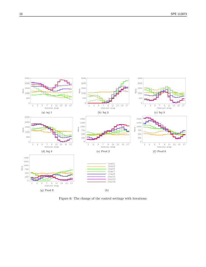
Fig. 6 shows the change of the control variables x` with iterations for several wells. The control settings atthe first iteration is very close to those used in the base case and they are gradually improved by the EnOpt. Thechanges to the controls are relatively large at the early iterations, and the control settings tend to converge in thelater iterations.

Summary In this example, the reservoir properties were assumed to be known without uncertainty and the wellcontrols were optimized based on the true reservoir. The total water injection rate and the total fluid production ratewere redistributed among the wells to maximize the NPV at the end of life of the reservoir. The major contributionof the optimization in this particular example was reducing water production and the NPV was increased by 3.6%from the base case. The amount of increase of the NPV and the optimized control settings depend on the choice ofthe parameters used in the calculation of the NPV. If the cost of the water disposal is much higher than the one usedin this example, the optimized control setting shows more tendency to reduce water production and the percentageincrease of the NPV is much higher compared to the current example due to larger benefit of the reduction ofproducing water.

10 SPE 112873

1 3 5 7 9 11 13 15 17Control step

0

500

1000

1500

2000

2500

Rate

(a) inj 1

1 3 5 7 9 11 13 15 17Control step

0

500

1000

1500

2000

2500Rate

(b) Inj 2

1 3 5 7 9 11 13 15 17Control step

0

500

1000

1500

2000

2500

Rate

(c) Inj 3

1 3 5 7 9 11 13 15 17Control step

0

500

1000

1500

2000

2500

Rate

(d) Inj 4

1 3 5 7 9 11 13 15 17Control step

0

250

500

750

1000

1250

1500

Rate

(e) Prod 2

1 3 5 7 9 11 13 15 17Control step

0

250

500

750

1000

1250

1500

Rate

(f) Prod 6

1 3 5 7 9 11 13 15 17Control step

0

250

500

750

1000

1250

1500

Rate

(g) Prod 9

iter1iter3iter5iter7iter9iter11iter13iter15

(h)

Figure 6: The change of the control settings with iterations.

SPE 112873 11

This first example investigated the idealized situation in which there is no uncertainty in the geological prop-erties; it will be referred to as optimization with known geology. Closed-loop optimization requires both theoptimization of control variables and the estimation of properties of the reservoir model. Only the EnOpt is testedby this example where it showed reasonable results. The use of the EnOpt as an integral part of the ensemble-basedclosed-loop optimization will be examined in the next example.

Ensemble-based closed-loop optimization In this example we consider a reservoir of size 2050 × 2050 ft2,uniformly discretized into 41 × 41 square cells. The net pay thickness is 40 ft. We assume only two phases, oiland water, are present. The irreducible water saturation and the residual oil saturation are both 0.2. Capillarityis neglected. Initially the reservoir is saturated with oil and irreducible water. We assume the north and the southsides are no-flow boundaries and permeability, which is to be estimated by incorporating the production data, isthe only uncertain geological property. The reference log transformed permeability field, ln k, used to generate thesynthetic production data is shown in Fig. 7. The major feature of this reservoir is a high permeability streakcrossing in the main flow direction. The reservoir is completed with a horizontal injector on the west side and ahorizontal producer on the east side. Both the injector and the producer are composed of ten equal-length segmentswith control valves on every segment. The injection and production rate through each segment can be monitoredand controlled. The control parameters in this case are the degree of opening of each control valve. The location ofthe valves are shown in Fig. 7 with triangles and half circles for the producer and the injector, respectively. Theyare numbered from one to ten.

9.08.37.56.86.15.44.63.93.22.51.71.0

ProducerInjector

P10

P6

P2

P8

P4

P9

P1

P5

P7

P3

I10

I6

I2

I8

I4

I9

I1

I5

I7

I3

Figure 7: The reference ln k field, and the location of the control valves.

The horizontal injector is controlled by water injection rate of 4100 stb/day. The horizontal producer iscontrolled by bottom hole pressure of 2000 psi. The simulation lasts 1140 days that is roughly the period forinjecting one pore volume of water based on the total injection rate constraint (4100 stb/day). The objective is tomaximize the NPV by the end of 1140 days. The price of oil is $70/bbl and the cost of water disposal is $5/bbl.Zero discount rate is used in this example. The control settings are adjusted every two months, thus the numberof control steps is 19 and the number of control parameters is 380. The production data available include waterrate through each injector segment, oil and water production rates through each producer segment and the bottomhole pressure of the injector. These production data are assumed to be available at day 30, 90, 270 and 450. 60realizations are used in this example.

Results and discussions We compare four different control scenarios in this example:

1. No-control: All the segments are fully open.

2. Reactive control: All the segments are fully open initially and the segments are subsequently closed accordingto the water oil ratio.

3. Optimization with known geology: The reservoir geological properties are assumed to be known withoutuncertainty and the production optimization is done based on the “true” reservoir.

4. Closed-loop optimization: The reservoir gridblock permeability is assumed to be uncertain. The EnKF isused to improve the estimation of the permeability. The valve settings are optimized under the uncertainreservoir description through the EnOpt.

12 SPE 112873

The first two scenarios serve as base cases. The no-control case represents the situation where no controlvalves are available. The reactive control case changes the valve settings by merely reacting to the productionresponses from the true reservoir. It mimics the typical remedy taken in the field without the help of model-basedoptimization techniques. The third case, optimization with known geology represents the same situation as theprevious example where the reservoir properties are assumed to be known. The optimization with known geologycase serves as a reference, to which we can compare the results of the closed-loop optimization.

Closed-loop optimization with uncertain geology is the focus of this example. The EnKF updates the estimateof the permeability field and the EnOpt optimizes the valve settings based on the latest estimate of the permeabilityfield. We could expect that if the closed-loop optimization did well, the NPV earned in the closed-loop optimizationcase should be similar to that earned in the case of optimization with known geology. In the closed-loop optimization,initially all the segments are fully open, and the production optimization starts after the assimilation of the first setof production data at day 30. The production optimization is repeated after each update of the geological modeland the optimized control settings are expected to be more appropriate for the true reservoir with better predictionof the reservoir responses provided by the updated reservoir model.

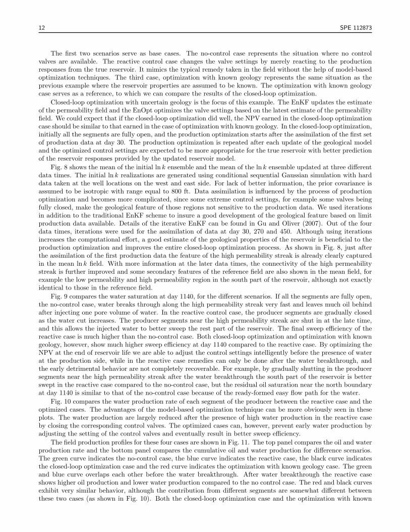
Fig. 8 shows the mean of the initial ln k ensemble and the mean of the ln k ensemble updated at three differentdata times. The initial ln k realizations are generated using conditional sequential Gaussian simulation with harddata taken at the well locations on the west and east side. For lack of better information, the prior covariance isassumed to be isotropic with range equal to 800 ft. Data assimilation is influenced by the process of productionoptimization and becomes more complicated, since some extreme control settings, for example some valves beingfully closed, make the geological feature of those regions not sensitive to the production data. We used iterationsin addition to the traditional EnKF scheme to insure a good development of the geological feature based on limitproduction data available. Details of the iterative EnKF can be found in Gu and Oliver (2007). Out of the fourdata times, iterations were used for the assimilation of data at day 30, 270 and 450. Although using iterationsincreases the computational effort, a good estimate of the geological properties of the reservoir is beneficial to theproduction optimization and improves the entire closed-loop optimization process. As shown in Fig. 8, just afterthe assimilation of the first production data the feature of the high permeability streak is already clearly capturedin the mean ln k field. With more information at the later data times, the connectivity of the high permeabilitystreak is further improved and some secondary features of the reference field are also shown in the mean field, forexample the low permeability and high permeability region in the south part of the reservoir, although not exactlyidentical to those in the reference field.

Fig. 9 compares the water saturation at day 1140, for the different scenarios. If all the segments are fully open,the no-control case, water breaks through along the high permeability streak very fast and leaves much oil behindafter injecting one pore volume of water. In the reactive control case, the producer segments are gradually closedas the water cut increases. The producer segments near the high permeability streak are shut in at the late time,and this allows the injected water to better sweep the rest part of the reservoir. The final sweep efficiency of thereactive case is much higher than the no-control case. Both closed-loop optimization and optimization with knowngeology, however, show much higher sweep efficiency at day 1140 compared to the reactive case. By optimizing theNPV at the end of reservoir life we are able to adjust the control settings intelligently before the presence of waterat the production side, while in the reactive case remedies can only be done after the water breakthrough, andthe early detrimental behavior are not completely recoverable. For example, by gradually shutting in the producersegments near the high permeability streak after the water breakthrough the south part of the reservoir is betterswept in the reactive case compared to the no-control case, but the residual oil saturation near the north boundaryat day 1140 is similar to that of the no-control case because of the ready-formed easy flow path for the water.

Fig. 10 compares the water production rate of each segment of the producer between the reactive case and theoptimized cases. The advantages of the model-based optimization technique can be more obviously seen in theseplots. The water production are largely reduced after the presence of high water production in the reactive caseby closing the corresponding control valves. The optimized cases can, however, prevent early water production byadjusting the setting of the control valves and eventually result in better sweep efficiency.

The field production profiles for these four cases are shown in Fig. 11. The top panel compares the oil and waterproduction rate and the bottom panel compares the cumulative oil and water production for difference scenarios.The green curve indicates the no-control case, the blue curve indicates the reactive case, the black curve indicatesthe closed-loop optimization case and the red curve indicates the optimization with known geology case. The greenand blue curve overlaps each other before the water breakthrough. After water breakthrough the reactive caseshows higher oil production and lower water production compared to the no control case. The red and black curvesexhibit very similar behavior, although the contribution from different segments are somewhat different betweenthese two cases (as shown in Fig. 10). Both the closed-loop optimization case and the optimization with known

SPE 112873 13

x

y

0 500 1000 1500 20000

500

1000

1500

2000

9.08.37.56.86.15.44.63.93.22.51.71.0

(a) Initial

x

y

0 500 1000 1500 20000

500

1000

1500

2000

9.08.37.56.86.15.44.63.93.22.51.71.0

(b) Day 30

x

y

0 500 1000 1500 20000

500

1000

1500

2000

9.08.37.56.86.15.44.63.93.22.51.71.0

(c) Day 90

x

y

0 500 1000 1500 20000

500

1000

1500

2000

9.08.37.56.86.15.44.63.93.22.51.71.0

(d) Day 450

Figure 8: Mean of the initial ln k ensemble and mean of ln k ensemble updated at three different data times.

14 SPE 112873

x

y

0 500 1000 1500 20000

500

1000

1500

2000

0.800.750.690.640.580.530.470.420.360.310.250.20

(a) No-control

x

y

0 500 1000 1500 20000

500

1000

1500

2000

0.800.750.690.640.580.530.470.420.360.310.250.20

(b) Reactive

x

y

0 500 1000 1500 20000

500

1000

1500

2000

0.800.750.690.640.580.530.470.420.360.310.250.20

(c) Closed-loop

x

y

0 500 1000 1500 20000

500

1000

1500

2000

0.800.750.690.640.580.530.470.420.360.310.250.20

(d) Opt with known geology

Figure 9: Water saturation at day 1140 for different scenarios.

0 200 400 600 800 1000Time HdayL

0

500

1000

1500

2000

WPRHstb�dayL

(a) Reactive

0 200 400 600 800 1000Time HdayL

0

500

1000

1500

2000

WPRHstb�dayL

(b) Closed-loop

0 200 400 600 800 1000Time HdayL

0

500

1000

1500

2000

WPRHstb�dayL

(c) Opt with known geology

seg 1seg 2seg 3seg 4seg 5seg 6seg 7seg 8seg 9seg 10

(d)

Figure 10: Water production rate from each segment of the producer for different scenarios.

SPE 112873 15

geology case show much higher oil production at early time. The optimized control settings at each data timevary in the closed-loop optimization since the optimization is performed based on the geological model updatedat different data times, and the production profiles show some sudden changes at the data assimilation time dueto the change of the well constraints. In general the closed-loop optimization performed well and the results arecomparable with the case where the geological properties are assumed to be known.

The optimized control settings computed at subsequent data assimilation times result in a gradual increase inthe NPV, if applied to the true field. But the amount of increase is not very large, because the high permeabilitystreak feature of this reservoir is relatively simple and the main feature is captured by only incorporating theproduction data at the first data time. The NPV earned in the closed-loop optimization case is very close to thatearned in the case of optimization with known geology, as seen by the similar cumulative oil and water productionprofiles in Fig. 11. The NPV is increased by 254% from the no control case and 22% from the reactive control case.

0 200 400 600 800 1000Time HdayL

1000

2000

3000

4000

OPRHstb�dayL

(a) Field oil production rate

0 200 400 600 800 1000Time HdayL

0

1000

2000

3000

WPRHstb�dayL

(b) Field water production rate

0 200 400 600 800 1000Time HdayL

0

500000

1´106

1.5´106

2´106

OPTHstbL

(c) Cumulative oil production

0 200 400 600 800 1000Time HdayL

0

1´106

2´106

3´106

WPTHstbL

(d) Cumulative water production

Figure 11: Comparison of the field production responses among different cases: no control (green); reactive (blue);closed-loop (black); optimization with known geology (red).

To show the quality of the estimate of the permeability field we compare the production responses using theoptimized controls with the initial permeability ensemble and the permeability ensemble updated at day 450.Production responses from the initial reservoir ensemble are shown in Fig. 12 and the corresponding productionresponses from the ensemble updated at day 450 are shown in Fig. 13. The red curve indicates the referenceproduction responses and the gray box plot shows the statistics from the ensemble forecast. The box contains50% probability, the horizontal line in the box indicates the median and the whiskers indicate the maximum andthe minimum values. It is obvious that the predictions based on the initial ensemble are very different from thereference production responses and show very high uncertainty, while the predictions from the updated permeabilityensemble show better match to the data (production data at day 30, 90, 270 and 450) and better predictability.Note the data assimilation only utilized production data up to day 450, and no information from the rest of theproduction was used.

ConclusionsAn ensemble-based closed-loop optimization is proposed in this paper. It combines the ensemble Kalman

filter (EnKF) or an iterative method, the ensemble randomized maximum likelihood method (EnRML), with anew ensemble-based production optimization method (EnOpt). The EnKF has been used as an alternative to the

16 SPE 112873

50 250 450 650 850 1050Time HdayL

5001000150020002500300035004000

OPRHstb�dayL

(a) OPR

50 250 450 650 850 1050Time HdayL

0

250

500

750

1000

1250

1500

1750OPRp05Hstb�dayL

(b) OPR p05

50 250 450 650 850 1050Time HdayL

0

200

400

600

800

1000

1200

1400

OPRp08Hstb�dayL

(c) OPR p08

50 250 450 650 850 1050Time HdayL

0500100015002000250030003500

WIRI08Hstb�dayL

(d) WIR I08

50 250 450 650 850 1050Time HdayL

0

500

1000

1500

2000

2500

WPRp01Hstb�dayL

(e) WPR p01

50 250 450 650 850 1050Time HdayL

0

50

100

150

WPRp02Hstb�dayL

(f) WPR p02

50 250 450 650 850 1050Time HdayL

0

0.2

0.4

0.6

0.8

WCTp02

(g) WCT p02

50 250 450 650 850 1050Time HdayL

0

0.2

0.4

0.6

0.8

WCTp05

(h) WCT p05

50 250 450 650 850 1050Time HdayL

0

0.2

0.4

0.6

0.8

WCTp10

(i) WCT p10

Figure 12: Data match from the initial ensemble.

SPE 112873 17

50 250 450 650 850 1050Time HdayL

5001000150020002500300035004000

OPRHstb�dayL

(a) OPR

50 250 450 650 850 1050Time HdayL

0

250

500

750

1000

1250

1500

1750OPRp05Hstb�dayL

(b) OPR p05

50 250 450 650 850 1050Time HdayL

0

200

400

600

800

1000

1200

1400

OPRp08Hstb�dayL

(c) OPR p08

50 250 450 650 850 1050Time HdayL

0500100015002000250030003500

WIRI08Hstb�dayL

(d) WIR I08

50 250 450 650 850 1050Time HdayL

0

500

1000

1500

2000

2500

WPRp01Hstb�dayL

(e) WPR p01

50 250 450 650 850 1050Time HdayL

0

50

100

150

WPRp02Hstb�dayL

(f) WPR p02

50 250 450 650 850 1050Time HdayL

0

0.2

0.4

0.6

0.8

WCTp02

(g) WCT p02

50 250 450 650 850 1050Time HdayL

0

0.2

0.4

0.6

0.8

WCTp05

(h) WCT p05

50 250 450 650 850 1050Time HdayL

0

0.2

0.4

0.6

0.8

WCTp10

(i) WCT p10

Figure 13: Data match from the ensemble updated at day 450.

18 SPE 112873

traditional history matching method for several years and shown to be efficient and relatively robust. We found thatit was sometimes beneficial to use the EnRML (Gu and Oliver, 2007) to improve the estimation of the uncertaingeological properties. The EnOpt is used to adjust the production control variables to optimize the net presentvalue over the uncertain reservoir description.

The sensitivities needed in the data assimilation and the production optimization are approximated from theensemble in a very straightforward manner without the need for adjoint computation. The ensemble-based closed-loop optimization is very flexible since it is independent of the choice of the reservoir simulator and the financialmodel, thus it can be easily combined with any reservoir simulator and financial model with very limited amount ofcode development. The efficiency of this closed-loop optimization method results from the use of small ensemblesof realizations for data assimilation and production optimization. The ensemble-based closed-loop optimizationis also well suited to parallel computation. Based on current experience, 60 realizations appears to be enoughfor practical implementations. If necessary, the ensemble approximation can be further improved by intelligentlyselecting the initial ensemble and using localization to reduce the spurious correlation.

In the ensemble-based closed-loop optimization, we optimize the control variables with consideration of theuncertain description the geological properties. The uncertainty of the geological model is provided by the EnKFthrough an ensemble of plausible reservoir models. By choosing the expectation of the net present value to be theobjective, the ensemble-based closed-loop optimization is fairly robust to uncertainty in reservoir description.

The applicability of the EnOpt and the ensemble-based closed-loop optimization is assessed through the useof two synthetic examples. In the first example, the well controls are optimized by the EnOpt based on a knownchannelized reservoir model. The results showed the ability of the EnOpt to improve reservoir management inthe presence of complex geological features. The ensemble-based closed-loop optimization is demonstrated in thesecond example and the results are compared with other alternative control scenarios. A good estimate of thepermeability field, which captured the main features of the reference field, was obtained through the EnRML. Thenet present value of the field is significantly increased by the closed-loop optimization and the level of increase iscomparable with the hypothetical case where the optimization is performed with known geology.

AcknowledgmentWe acknowledge the financial support of the member companies of the OU Consortium on Ensemble Methods.

Multiple licenses of ECLIPSE were donated by Schlumberger. Computational resources were provided by the OUSupercomputing Center for Education and Research.

ReferencesAgbalaka, C. C., Oliver, D. S., 2007. Application of the EnKF and localization to automatic history matchingof facies distribution and production data. Math geology , accepted.

Arroyo-Negrete, E., Devegowda, D., Datta-Gupta, A., Choe, J., 2006. Streamline assisted ensemble Kalmanfilter for rapid and continuous reservoir model updating (SPE 104255). In: Proc. of the International Oil & GasConference and Exhibition in China, 5-7 December 2006, Beijing, China.

Bertino, L., Evensen, G., Wackernagel, H., 2003. Sequential data assimilation techniques in oceanography.International Statistical Review 71 (2), 223–241.

Brouwer, D. R., Nævdal, G., Jansen, J. D., Vefring, E. H., van Kruijsdijk, C. P. J. W., 2004. Improved reservoirmanagement through optimal control and continuous model updating. In: SPE Annual Technical Conferenceand Exhibition, 26-29 September, Houston, Texas.

Burgers, G., van Leeuwen, P. J., Evensen, G., 1998. Analysis scheme in the ensemble Kalman filter. MonthlyWeather Review 126, 1719–1724.

Chen, Y., Oliver, D. S., Zhang, D., 2007. Data assimilation for nonlinear problems by ensemble Kalman filterwith reparameterization. Journal of Petroleum Science and Engineering , submitted.

Chen, Y., Zhang, D., 2006. Data assimilation for transient flow in geologic formations via ensemble Kalmanfilter. Advances in Water Resources 29 (8), 1107–1122.

Evensen, G., 1994. Sequential data assimilation with a nonlinear quasi-geostrophic model using Monte Carlomethods to forecast error statistics. Journal of Geophysical Research 99 (C5), 10143–10162.

SPE 112873 19

Evensen, G., 2003. The ensemble Kalman filter: Theoretical formulation and practical implementation. OceanDynamics 53, 343–367.

Gu, Y., Oliver, D. S., 2005. History matching of the PUNQ-S3 reservoir model using the ensemble Kalman filter.SPE Journal 10 (2), 51–65.

Gu, Y., Oliver, D. S., 2007. An iterative ensemble Kalman filter for multiphase fluid flow data assimilation. SPEJournal 12 (4), 438–446.

Hamill, T. M., Whitaker, J. S., 2001. Distance-dependent filtering of background error covariance estimates inan ensemble Kalman filter. Monthly Weather Review 129 (11), 2776–2790.

Haugen, V., Natvik, L.-J., Evensen, G., Berg, A., Flornes, K., Nævdal, G., 2006. History matching using theensemble Kalman filter on a North Sea field case (SPE-102430). In: SPE Annual Technical Conference andExhibition.

Houtekamer, P. L., Mitchell, H. L., 2001. A sequential ensemble Kalman filter for atmospheric data assimilation.Monthly Weather Review 129 (1), 123–137.

Li, G., Reynolds, A., 2007. An iterative ensemble Kalman filter for data assimilation, SPE-109808. In: Proceedingof 2007 SPE Annual Technical Conference and Exhibition.

Li, R., Reynolds, A. C., Oliver, D. S., 2003. History matching of three-phase flow production data. SPE Journal8 (4), 328–340.

Liu, N., Oliver, D. S., 2005. Ensemble Kalman filter for automatic history matching of geologic facies. Journalof Petroleum Science and Engineering 47 (3–4), 147–161.

Lorentzen, R. J., Berg, A. M., Nævdal, G., Vefring, E. H., 2006. A new approach for dynamic optimizationof waterflooding problems, SPE-99690. In: Proceedings of the 2006 SPE intelligent energy conference andExhibition.

Mitchell, H. L., Houtekamer, P. L., Pellerin, G., 2002. Ensemble size, balance, and model-error representationin an ensemble Kalman filter. Monthly Weather Review 130 (11), 2791–2808–433.

Nævdal, G., Johnsen, L. M., Aanonsen, S. I., Vefring, E. H., 2005. Reservoir monitoring and continuous modelupdating using ensemble Kalman filter. SPE Journal 10 (1), 66–74.

Oliver, D. S., 1995. Moving averages for Gaussian simulation in two and three dimensions. Mathematical Geology27 (8), 939–960.

Sarma, P., Aziz, K., Durlofsky, L., 2005a. Implementation of adjoint solution for optimal control of smart wells,SPE-92864.

Sarma, P., Durlofsky, L., Aziz, K., 2005b. Efficient closed-loop production optimization under uncertainty,SPE-94241.

Tarantola, A., 2005. Inverse Problem Theory: Methods for Data Fitting and Model Parameter Estimation.Elsevier, Amsterdam, The Netherlands.

Van Doren, J. F. M., Van den Hof, P. M. J., Jansen, J. D., Bosgra, H., 2008. Determining identifiable parame-terizations for large-scale physical models in reservoir engineering. In: Proceedings of the 17th Int. Fed. Autom.Control (IFAC) World Congress, Seoul, Korea, July 6–11.

van Essen, G., Zandvliet, M., van den Hof, P., Bosgra, O., Jansen, J., 2006. Robust waterflooding optimizationof multiple geological scenario, SPE-102913. In: Proceedings of the 2006 SPE Annual Technical Conference andExhibition.

Wang, C., Li, G., Reynolds, A. C., 2007. Production optimization in closed-loop reservoir management, SPE109805. In: 2007 SPE Annual Technical Conference and Exhibition.