stability and robustness of large platoons of …plaza.ufl.edu/hehao/papers/rnc.pdfacting on all the...

INTERNATIONAL JOURNAL OF ROBUST AND NONLINEAR CONTROLInt. J. Robust. Nonlinear Control2012;00:1–26Published online in Wiley InterScience (www.interscience.wiley.com). DOI: 10.1002/rnc

Stability and robustness of large platoons of vehicles withdouble-integrator models and nearest neighbor interaction

He Hao∗, Prabir Barooah

SUMMARY

We study the stability and robustness of a large platoon of vehicles, where each vehicle is modeledas a double integrator, for two decentralized control architectures: predecessor-following and symmetricbidirectional. In the predecessor-following architecture, the control action on each agent only depends on theinformation from its immediate front neighbor, while in thesymmetric bidirectional architecture, it dependsequally on the information from both its immediate front neighbor and back neighbor. We prove asymptoticstability of the formation for a class of nonlinear controllers with sector nonlinearity, with the linearcontroller as a special case. We show the convergence rate ofthe predecessor-following architecture is muchfaster than that of the symmetric bidirectional architecture. However, the predecessor-following architecturesuffers high algebraic growth of initial errors. We also establish scaling laws (withN) of certainH∞norms of the formation that measure its robustness to external disturbances for the linear case. It is shownthat the robustness performance grows geometrically inN for predecessor-following architecture, but onlypolynomially inN for symmetric-bidirectional architecture. Extensive numerical simulations are conductedto verify the predictions for the linear case and empirically estimate the corresponding performance metricsfor a saturation-type nonlinear controller. Based on the analytical and numerical results, it is seen that thesymmetric bidirectional architecture outperforms the predecessor-following architecture in all measures ofperformance. Within the predecessor-following architecture, the non-linear controller is seen to performbetter in general than the linear one. A number of design guidelines are provided based on these conclusions.Copyright c© 2012 John Wiley & Sons, Ltd.

Received . . .

KEY WORDS: Multi-agent systems; Convergence rate;H∞ norm; Nonlinear control; Distributed control

1. INTRODUCTION

Cooperative control of multi-agent systems has spurred an extensive interest in the controlcommunity because of its wide range of applications such as automated highway system [1, 2],coordination of aerial, ground, and autonomous vehicles for surveillance and rescue [3], spacecraftformation control for science missions [4], and collective behavior of bird flocks and animalswarms [5]. Among these applications, one of the most well studied problems is autonomousintelligent cruise control of large vehicular platoons, see [6, 7, 8, 9] and the reference therein. Theprimary goal of autonomous intelligent cruise control is toincrease traffic throughput and safety.

One of the most important problems in autonomous intelligent cruise control of platoons is stringinstability or slinky-type effect [10, 11, 12]. To solve this problem, different control policies andcontrol architectures are considered. In [11], a constant headway control law is developed to insurestring stability. However, the constant headway policy by itself is not enough, the headway has

∗Correspondence to: He Hao. He Hao and Prabir Barooah are withDepartment of Mechanical and AerospaceEngineering, University of Florida, Gainesville, FL 32611, USA. Email:hehao,[email protected]. This work wassupported by the National Science Foundation through Grants CNS-0931885 and ECCS-0925534.

Copyright c© 2012 John Wiley & Sons, Ltd.

Prepared usingrncauth.cls [Version: 2010/03/27 v2.00]

2

to be large enoughto avoid the problems associated with constant spacing policy [13]. Sinceone of the main motivations for automated platooning is to achieve higher highway capacity bymaking cars move with a small inter-vehicle separation, there is a need to study the constantspacing policy. In was shown in [11, 14, 15] that with constant spacing policy, the leader’sinformation need to be broadcasted to the following vehicles to assure string stability. Nevertheless,the inevitable time delay and package drop in broadcasting the leader’s information will cause stringinstability [16]. This leads to the study of decentralized control architecture, i.e. each vehicle canonly use measurements of relative position and/or velocitywith respect to its nearest neighbors.

Two decentralized control architectures that are commonlyexamined are predecessor-followingand bidirectional architectures. In thepredecessor-followingarchitecture, the control action on eachvehicle only depends on the relative information from its immediate predecessor, i.e. the vehicle infront of it. In the bidirectional architecture, the controldepends on the relative information from bothits immediate predecessor and follower. Within the bidirectional architecture, the most commonlyanalyzed case is thesymmetric bidirectionalarchitecture, in which the control at a vehicle dependson the information from both of its neighborsequally.

A typical issue in distributed/decentralized control is that as the number of agents in the systemincreases, the performance of the closed-loop degrades progressively. It has been established thatthe predecessor-following architecture suffers from highsensitivity to external disturbances withlinear control [17, 18]. High sensitivity to external disturbance is typically referred to as slinky-type effect [19, 20] or string instability [21]. Seileret al.showed that with linear control, the poorrobustness performance with the predecessor-following architecture is independent of the design ofthe controller, but a fundamental artifact of the architecture [14]. The robustness performance canbe improved by non-identical linear controllers but at the expense of the control gains increasingwithout bound as the number of the vehicles increases [11, 22]. It was shown in [14, 23, 15, 21] thatthe symmetric bidirectional architecture also suffers from poor sensitivity to external disturbances.

Although a rich literature exist on sensitivity to disturbances for predecessor-following andsymmetric bidirectional architectures with linear control, to the best of our knowledge, a precisecomparison of these two architectures is lacking. Moreover, most of the works on formation controlhave been limited to linear control laws, while little is known about nonlinear control. Nonlinearterms in the closed loop dynamics may arise from either purposefully designed nonlinear controllaws (if beneficial) or unavoidable non-linearities in the agent dynamics, such as actuator saturation.Both of these cases can be analyzed by considering linear plant dynamics and nonlinear controllers.

In this paper we examine the stability and robustness (sensitivity to external disturbances) oflarge platoon of vehicles with linear as well as a class of nonlinear controllers, for both predecessor-following and symmetric bidirectional architectures. Each vehicle is modeled as a fully actuatedpoint mass (double-integrator). A few authors have used first order kinematic models by ignoringvehicle inertia. However, in general kinematic models (single integrator) fail to reproduce the slinky-type effects that are exhibited by kinetic models (double integrator).

We prove stability of the closed loop with an arbitrary number of agents for a class of non-linear controllers where the control gain functions satisfy certain sector conditions. The differencebetween the transient responses of the two architectures incase of linear control is explainedby the expressions we derive for the least stable eigenvalueof the closed-loop state matrix andits multiplicity. In particular, we show that the predecessor-following architecture has a largerconvergence rate compared to the symmetric bidirectional architecture:O(1) vs. O(1/N2). Itis worthwhile to mention the convergence rate of the formation with symmetric bidirectionalarchitecture scales poorly as a function ofN even with centralized LQR control [24]. The realpart of the least stable eigenvalue with LQR control scales asO(1/N). However, the predecessor-following architecture suffers from algebraic growth of initial conditions due to the high multiplicityof the least stable eigenvalue. For the non-linear control,we study the transient performance throughnumerical simulations. The simulations show that in the predecessor-following architecture, thetransient response is significantly improved by using a saturation-type non-linearity in the controlgain instead of a linear control.

Copyright c© 2012 John Wiley & Sons, Ltd. Int. J. Robust. Nonlinear Control(2012)Prepared usingrncauth.cls DOI: 10.1002/rnc

3

Next, we examine the closed-loop’s performance in terms of the sensitivity to externaldisturbances. Specifically, we examine thefirst-to-last amplification factor, defined as theL2

gain from a disturbance injected at the first vehicle to the position tracking error of the lastvehicle andall-to-all amplification factor, which is defined as theL2 gain from the disturbancesacting on all the vehicles to their position tracking errors. In case of linear controllers, we showthat whenN is large, the first-to-last amplification factor, which becomes aH∞ norm, growsasO(αN ), α > 1, for predecessor-following architecture but only asO(N) for the symmetricbidirectional architecture. The all-to-all amplificationfactor scales asO(αN ) for predecessor-following architecture while asO(N3) for the symmetric bidirectional architecture. The first resultis known in the literature [14]. These results establish a precise comparison between therobustnessof symmetric bidirectional and predecessor-following architectures with linear control. Namely,symmetric bidirectional architecture has a much smaller sensitivity to external disturbances.

Establishing scaling laws for robustness metrics with non-linear controllers is challenging.We therefore study the response in the non-linear case through extensive numerical simulations,with both sinusoidal and random disturbances as inputs, andestimate performance metrics fromsimulation data. We observe from these studies that, withinthe predecessor-following architecture,a nonlinear controller with a saturation-type non-linearity performs better than the correspondinglinear one. In the symmetric bidirectional architecture, the difference between the linear andnonlinear controller’s performance is not significant.

The theoretical as well as numerical simulations lead to certain design guidelines. Comparingall four combinations (linear, non-linear, predecessor following and symmetric bidirectional), weobserve that for the same number of agents, the symmetric bidirectional architecture performsconsiderably better (both in terms of transient decay and robustness to disturbances) than thepredecessor following one, and this conclusion is valid forboth the linear and non-linear controllaws. Thus, the added complexity and cost of the symmetric bidirectional architecture due toadditional sensors is justified. If stringent cost considerations allow only the predecessor followingarchitecture, then the non-linear controller should be used over the linear one. Even with a linearcontrol law actuator saturation will make the overall system closer to the closed loop non-linearsystem studied. Therefore, the fact that both the linear andnonlinear controllers with sectornonlinearities are seen to perform comparably in the symmetric bidirectional architecture can beseen as a “robustness to modeling errors” of this architecture. Some of the results for the linearpredecessor following case may be known or easily derived from existing results. We neverthelessinclude them for the sake of completeness.

The conclusions about the architectures are derived only for the specific control laws weinvestigated. The local control laws at the vehicles are either of PD (proportional-derivative) type(in the linear case), or such that their linearization around the origin are of PD-type (in the non-linear case). Nevertheless, analysis carried out with thiscontroller structure and double integratorvehicle models is relevant even if there are additional dynamic elements in the loop (i.e, either inthe controller or in the vehicle dynamic model), at least in the linear case. Reasons for this can beseen from the results in [23], which considered vehicle models with two integrators in series with anadditional transfer function (to model powertrain dynamics) and arbitrary LTI compensators. First,a dynamic controller cannot have a zero at the origin since itwill result in a pole-zero cancellationcausing the steady-state errors to grow without bound asN increases [23]. Second, a dynamiccontroller cannot have an integrator either if the vehicle model has two integrators. For if it does, theclosed-loop platoon dynamics become unstable for a sufficiently large values ofN [23]. As a result,any allowable dynamic element in the loop must essentially act as a static gain at low frequencies.The results of [23] indicate that the principal challenge in controlling a platoon of vehicles arisesdue to the presence of a double integrator with its unboundedgain at low frequencies. Hence, theissues discussed here with a PD controller structure is alsorelevant to the case where additionaldynamic elements appear in the loop.

In terms of the stability analysis with non-linear controllers, our work closely parallels thatof [25], which considers arbitrary information graphs (instead of the 1-D graph of a platoon weconsider). However, the results of [25] are not applicable to the scenario considered here, since we


4

...

O X∆(0,1)∆(N−1,N)

012N − 1N

Figure 1. Desired geometry of a 1-D network ofN double-integrator agents. The reference agent with index“0” need not to be real agent, it merely provides the reference trajectory of the formation to agent1.

consider relative velocity feedback while [25] considers absolute velocity feedback. Furthermore,the assumption of symmetry made in [25] precludes the predecessor-following architecture fromtheir formulation. In terms of sensitivity to external disturbances with linear control, our work isrelated to [26, 27, 28] and [29, 30]. In [26, 27], it is shown that if the information graph usedis undirected and has bounded degree, the maximum error due to sinusoidal disturbances can notbe made independent of the size of the formation. In [28], Veerman showed that the first-to-lastamplification grows linearly inN for the symmetric bidirectional case, but grows exponentially inN for asymmetricbidirectional architecture, where asymmetric means the information from its frontand back neighbor are weighted differently. Scaling laws ofcertainH2 norms from disturbance tooutputs that quantify a number of performance measures are examined in [29, 30]. In particular,it was shown that the “all-to-all”H2 norm scales exponentially inN for predecessor-followingarchitecture (although with absolute velocity feedback) [30], but asO(N3) for the symmetricbidirectional architecture [29], which is the same as that of the all-to-allH∞ norm established inthis paper. They also show that the scaling laws for theH2 norm hold for arbitrary but fixed numberof front and back neighbors and arbitrary stabilizing feedback gains.

The rest of this paper is organized as follows. Section2 presents the problem statement. Section3and Section4 present the stability and robustness analysis, respectively, along with correspondingnumerical studies. The paper ends with a summary in Section5.

2. PROBLEM STATEMENT

We consider the formation control ofN homogeneous agents which are moving in 1-D Euclideanspace, as shown in Figure1. The position of thei-th agent is denoted bypi and each agent is modeledas a double integrator:

pi = ui + wi, i ∈ {1, 2, · · · , N}, (1)

whereui is the control input, andwi is the external disturbance. This is a commonly used modelfor vehicle dynamics in studying vehicular platoons, and results from feedback linearization of non-linear vehicle dynamics [11, 31].

The control objective is to make the network of agents maintain a rigid formation geometrywhile following a desired trajectory. The desired geometryof the formation is specified by thedesired gaps∆(i−1,i) for i ∈ {1, · · · , N}, where∆(i−1,i) is the desired value ofpi−1(t) − pi(t).The desired inter-vehicular gaps∆(i−1,i)’s are positive constants and they have to be specified in amutually consistent fashion,∆(i,k) = ∆(i,j) + ∆(j,k) for every triple(i, j, k) wherei ≤ j ≤ k. Thedesired trajectory of the formation is provided in terms of afictitiousreference agent with index0,whose trajectory is denoted byp∗0(t). The information on the desired trajectory of the formationisonly provided to agent1. The desired trajectory of thei-th agent,p∗i (t), is given by

p∗i (t) = p∗0(t) − ∆(0,i) = p∗0(t) −i

∑

j=1

∆(j−1,j). (2)

In this paper, we consider the following twodecentralizedcontrol architectures:

1. Predecessor-following architecture. The control action at thei-th agent depends on the relativeposition and velocity measurements from its immediate front neighbor. In particular, we


5

consider the following decentralized control law:

ui = − f(pi − pi−1 + ∆(i−1,i)) − g(pi − pi−1), (3)

wherei ∈ {1, 2, · · · , N} andf, g : R → R are scalar functions.2. Symmetric bidirectional architecture. The control action at thei-th agent depends on the

relative position and velocity measurements from its immediate front and back neighbors,and the information from its front and back neighbors are weighted equally. In particular, weconsider the following decentralized control law:

ui = − f(pi − pi−1 + ∆(i−1,i)) − g(pi − pi−1)

− f(pi − pi+1 − ∆(i,i+1)) − g(pi − pi+1),

uN = − f(pN − pN−1 + ∆(N−1,N)) − g(pN − pN−1), (4)

wherei ∈ {1, 2, · · · , N − 1} andf, g : R → R.

In both architectures, the information needed to compute the control action at each agent can beeasily obtained by on-board sensors such as radars, since only relative position and velocity areused in the control.

In this paper, we make the following assumptions.

Assumption 1In the above controllers (3) and (4), the possibly nonlinear functionsf, g : R → R are odd functions,which are smooth enough to guarantee the existence of solution of the coupled ODEs. Eachagenti knows the desired gaps∆(i−1,i), ∆(i,i+1), while only agent1 knows the desired trajectoryp∗0(t) of the fictitious reference agent. The reference trajectoryis a constant velocity type, i.e.,p∗0(t) = v0t+ c0 for some constantsv0, c0. The first agent must have access to its own absoluteposition and velocity information. 2

To facilitate analysis, we define the following position tracking error:

pi := pi − p∗i , (5)

wherep∗i is given by (2). The closed-loop dynamics for the predecessor-followingarchitecture cannow be expressed as the following coupled-ODE model

¨pi = − f(pi − pi−1) − g( ˙pi − ˙pi−1) + wi, i ∈ {1, 2, · · · , N}. (6)

The closed-loop dynamics for the symmetric bidirectional architecture are

¨pi = − f(pi − pi−1) − g( ˙pi − ˙pi−1) − f(pi − pi+1) − g( ˙pi − ˙pi+1) + wi, i < N,

¨pN = − f(pN − pN−1) − g( ˙pN − ˙pN−1) + wN . (7)

Note thatp0(t) = ˙p0(t) ≡ 0, since the reference agent perfectly tracks its desired trajectory. Thesystem can be expressed in the state space form:

x = f(x,w), (8)

where the state and disturbance vectors are defined asx := [p1, ˙p1, · · · , pN , ˙pN ]T and w :=[w1, · · · , wN ]T . The special casef(z) = k0z andg(z) = b0z (wherez is the argument andk0 >0, b0 > 0) in the above coupled-ODEs correspond to the case oflinear control in each architecture.In the case of linear control, the closed-loop can be represented as:

x = Ax+Bw, (9)

whereA is the state matrix that depends onk0, b0 andB is the input matrix with appropriatedimension.

In this paper, we study the stability of the originx = 0 of the undisturbed systemx = f(x, 0)given in (8) with linear as well as a class of nonlinear controllers for two architectures. In addition,we examine the sensitivity of position tracking errorsp = [p1, · · · , pN ]T to the external disturbancesw = [w1, · · · , wN ]T .


6

3. STABILITY ANALYSIS

In this section, we present the stability analysis of the origin x = 0 of the undisturbed systemx = f(x, 0) given in (8) with both linear and nonlinear controllers. For the linearcase, we alsoderive formulae showing how the least stable eigenvalue of the state matrixA in (9) changes withincreasing size of the formation. This eigenvalue quantifies the system’s convergence rate withrespect to initial errors. For the case of non-linear controller, we provide sufficient conditionsfor asymptotic stability. Since convergence rates for non-linear systems are difficult to obtainanalytically, we perform numerical simulations to study the convergence rate with non-linearcontrollers and compare with corresponding linear controllers. All simulations for studying transientperformance correspond to the following scenario: the disturbance acting on each agent is zero; weperturb the initial position of the first agent from its desired value and observe the position trackingerror of the last agentpN(t). For the convenience of comparison, we define the following as ameasure of transient performance:

E := limT→∞

1

x20

∫ T

0

1

2k0p

2N (t) +

1

2˙p2N(t) dt. (10)

wherek0 > 0 is the linear position gain given as before andx0 is the initial error of the first agent:

p1(0) = x0. (11)

The quantityE is called theintegral of transient energy. We assume the limit in (10) exits, i.e. thelast agent has finiteL2 energy. In numerical simulations, we use the following estimate ofE,

E :=1

x20

∫ T

0

1

2k0p

2N (t) +

1

2˙p2N (t) dt, (12)

whereT is sufficiently large such that all the errors die out. We study through numerical simulationshowE scales with the number of agentsN and the initial errorx0.

3.1. Stability analysis with linear control

In the statement of the next theorem, theleast stable eigenvalueof a matrix refers to the eigenvaluewith the largest real part.

Theorem 1Consider a 1-D network ofN double-integrator agents with linear control law, i.e.f(z) = k0z,g(z) = b0z. If k0 > 0, b0 > 0, the closed-loop dynamics are exponentially stable for both thepredecessor-following and symmetric bidirectional architectures. Under the same conditions, thefollowing statements hold.

1. With predecessor-following architecture, the least stable eigenvalue of the closed-loop state

matrixA is µ1 =−b0+

√b20−4k0

2 , and this eigenvalue occurs with multiplicityN .2. With symmetric bidirectional architecture, whenN is large, the least stable eigenvalue is given

by µ1 = −π2b08N2 + ℑ, with multiplicity of 1, whereℑ is an imaginary number. 2

The first statement of the theorem seems to be well known in thecommunity; though we wereunable to find a reference for it. The proof of Theorem1 is given in the appendix.

Although stability guarantees that transients due to initial conditions decay to0 ast→ ∞, thespeed at which the transients decay depends quite strongly on the architecture and the controllerdesign. For a linear system, an appropriate measure of this convergence rate is the absolute value ofthe real part of the least stable eigenvalue of state matrixA, as long as the least stable eigenvalueis not repeated. If the least stable eigenvalue is repeated,then algebraic growth (peaking) occurs.In that case, the convergence rate is proportional totkeRe(µ1)t, wherek is the algebraic multiplicityof the least stable eigenvalueµ1. It follows from Theorem1 that the real part of the least stable


7

eigenvalueRe(µ1) in predecessor following architecture is independent ofN , while it decays to0with increasingN for symmetric bidirectional architecture. This makes the predecessor-followingarchitecture appear to have faster convergence rate than the symmetric bidirectional architecture,especially for largeN . However, the large algebraic multiplicity of the least stable eigenvalue in thepredecessor-following architecture will cause large algebraic growth of the initial conditions beforethey decay to0. Corroboration through numerical simulations is providedin Section3.3.

3.2. Stability analysis with non-linear control

The next two theorems are on the stability of the network withnon-linear controllers, their proofsare given in the appendix. In the statements of the theorems that follow we say that a scalar functionf belongs to the sector[ε,K] if εz2 ≤ zf(z) ≤ Kz2, ∀ z ∈ R, and it belongs to the sector(0,∞] ifzf(z) > 0, ∀ z 6= 0.

Theorem 2Consider a 1-D network of double-integrator agents with predecessor-following architecturewith controller (3). If f, g : R → R satisfy the sector conditionsf ∈ [ε1,K1], g ∈ [ε2,K2], where0 < ε1 ≤ K1 <∞, 0 < ε2 ≤ K2 <∞, then the originx = 0 of the undisturbed dynamicsx =f(x, 0) (8) is globally asymptotically stable. 2

Theorem 3Consider a 1-D network of double-integrator agents with symmetric bidirectional architecture withcontroller (4). If f, g : R → R satisfy the sector conditionsf ∈ (0,∞], g ∈ (0,∞], then the originx = 0 of the undisturbed dynamicsx = f(x, 0) (8) is globally asymptotically stable. 2

Remark 1Note that stability with the linear controllers are specialcases of Theorem2 and Theorem3.Comparing the above two theorems, we notice that the requirement on the sector condition inthe predecessor-following architecture is stricter than that of symmetric bidirectional architecture.However, these sector conditions are only sufficient. 2

3.3. Numerical comparison between linear and nonlinear controllers for transient decay

Since every practical actuator has saturation limits, saturation-type nonlinearity is of particularinterest. The saturation-type nonlinearity in controlling large platoon is practically important anddraws many researchers’ attention [32, 33]. Throughout this section, we consider the followingspecific linear and saturation-type nonlinear controllers. The control gain functionsf(z) andg(z)used in controllers (3) and (4) are given by

Linear:f(z) = k0z, g(z) = b0z,

Non-linear:f(z) = B1 tanh(γ1z), g(z) = B2 tanh(γ2z), (13)

wherek0 = 1, b0 = 0.5, B1 = 5, γ1 = 0.2, B2 = 5, γ2 = 0.1. The parameters have been chosen insuch a way that the slopes off(z) of g(z) near the origin are equal tok0 andb0, respectively. Thisis done to make the linear and non-linear cases comparable tosome extent. Note that thesef(z)andg(z) do not satisfy the sector conditions assumed in Theorem2 globally, but only satisfy thesector conditionslocally. However, the region in which they satisfy the sector condition can be madearbitrarily large by choosing sufficiently smallε1 andε2.

We compare the convergence rate and transient performance between linear and nonlinearcontrollers through numerical simulations. Figure2 (a) depicts the transients of the 1-D networkwith linear and nonlinear controllers for predecessor-following architecture. The algebraic growthfor linear controller which is predicted by Theorem1 is observed. We also see that the nonlinearcontroller has much smaller peak error than the linear controller. The transients in the symmetricbidirectional architecture are shown in Figure2 (b). We see that (i) the performance of the non-linear case is similar to that of the linear controller, and (ii) the peak value of the error is muchsmaller compared to that in the predecessor-following architecture, no matter the controller is linearor nonlinear.


8

0 100 200 300−2000

−1000

0

1000

2000

time (t)

pN

LinearNonlinear

(a) Predecessor-following

0 100 200 300−1.5

−1

−0.5

0

0.5

1

1.5

time (t)

pN

LinearNonlinear

(b) Symmetric bidirectional

Figure 2. Comparison of transients of the position trackingerror of the last agent for a network ofN = 10agents between linear and nonlinear controller. The initial condition of the first agent used isx0 = 10.

110 120 130 140 150 160−0.5

−0.4

−0.3

−0.2

−0.1

0

0.1

0.2

0.3

0.4

0.5

time (t)

pN

Linear predecessor-followingNonlinear predecessor-followingLinear symmetric bidirectionalNonlinear symmetric bidirectional

Figure 3. Comparison of convergence rate for a network ofN = 10 agents between predecessor-followingand symmetric bidirectional architectures. The initial condition of the first agent used isx0 = 10.

Figure 3 shows a “zoomed-in” version of the transient response. We see from the figure thatthe convergence rates of the linear and non-linear controllers in each architecture are similar. Inaddition, the error in the predecessor-following architecture is smaller than in the case of symmetricbidirectional architecture forlarget. This can be explained in the linear case from the real part oftheleast stable eigenvalue: it is much larger in the predecessor-following architecture compared to thesymmetric bidirectional architecture,O(1) vs.O(1/N2) (recall Theorem1). The similarity betweenthe simulation results in the non-linear and linear cases indicate that the convergence rate in thepredecessor-following architecture is higher than that inthe symmetric bidirectional one, whethercontrol is linear or nonlinear.

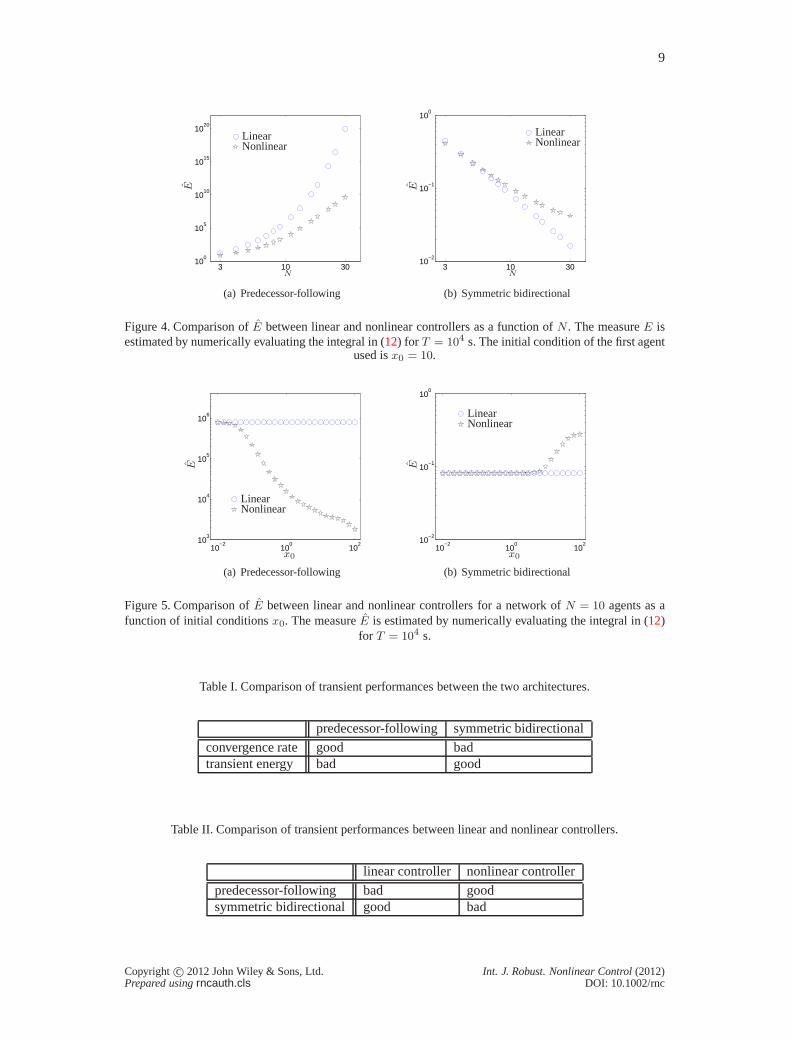
Figure 4 and Figure5 show the estimate of energy measureE for T = 104 seconds (definedin (12)) as a function ofN andx0 respectively. Recallx0 is the initial position error of the firstagent, it’s given in (11). We see that (i) the energy in the predecessor-following architecture has amuch worse scaling trend withN or x0 than that in symmetric bidirectional architecture, no matterthe controller is linear or nonlinear, (ii) nonlinear controller performs better than linear controller inthe predecessor-following architecture (Figure4 (a), Figure5 (a)), whereas it performs similarly orworse in the symmetric bidirectional architecture (Figure4 (b), Figure5 (b)).


9

3 10 3010

0

105

1010

1015

1020

E

N

LinearNonlinear


3 10 3010

−2

10−1

100

E

N

LinearNonlinear


Figure 4. Comparison ofE between linear and nonlinear controllers as a function ofN . The measureE isestimated by numerically evaluating the integral in (12) for T = 104 s. The initial condition of the first agent

used isx0 = 10.

10−2

100

10210

3

104

105

106

E

x0

LinearNonlinear


10−2

100

10210

−2

10−1

100

E

x0

LinearNonlinear


Figure 5. Comparison ofE between linear and nonlinear controllers for a network ofN = 10 agents as afunction of initial conditionsx0. The measureE is estimated by numerically evaluating the integral in (12)

for T = 104 s.

Table I. Comparison of transient performances between the two architectures.

predecessor-following symmetric bidirectionalconvergence rate good badtransient energy bad good

Table II. Comparison of transient performances between linear and nonlinear controllers.

linear controller nonlinear controller

predecessor-following bad goodsymmetric bidirectional good bad


10

3.4. Design guidelines based on transient response

Based on the numerical and analytical results, the comparisons of performance are summarized inTableI and TableII . It follows that the predecessor-following architecture has a faster convergencerate (good) but much higherintegral of transient energyE (bad) compared to the symmetricbidirectional architecture. These conclusions hold irrespective of whether the controller is linearor nonlinear, see Figure2-5. In fact the transients are so large with the predecessor-followingarchitecture that it is very likely to lead to collisions even for small initial errors. So if a designchoice is to be made among the two architectures, the symmetric bidirectional should be chosen.Within the bidirectional architecture, the linear controller seems to perform slightly better thanthe nonlinear one, so the linear controller should be chosen. If for some reason the predecessor-following architecture has to be used, the non-linear control law should be used since it clearlyoutperforms the linear one in terms of transient energy.

4. ROBUSTNESS (SENSITIVITY TO EXTERNAL DISTURBANCES)

In this section, we study the sensitivity of the network to external disturbances. Specifically, weexamine appropriate gains from (i) a disturbance on the firstagentw1 ∈ R to the position trackingerror of the last agentpN ∈ R, and (ii) disturbances acting on all agentsw ∈ R

N to the positiontracking errors of all agentsp ∈ R

N . Both sinusoidal and random disturbances are considered. Forthe first scenario, we consider the metricfirst-to-last amplification factor(AFTL), defined as theL2

gain from inputw1 to outputpN :

Alinear or nonlinearFTL = sup

‖pN‖L2(τ)

‖w1‖L2(τ), (14)

where theL2 norm in the expression above is defined in the extended space [34], i.e. ‖e‖L2(τ) :=√

∫ τ

0 ‖e(t)‖2dt for a large but finiteτ . In the linear case, denoting byGFTL(s) the SISO transfer

function fromw1 to pN , this is the same as theH∞ norm ofGFTL(s) [34], i.e.,

AlinearFTL = max

ω|GFTL(jω)| = |GFTL(jωp)|, whereωp := arg max

ω|GFTL(jω)|, (15)

where we have assumed for the moment that the maximum is achieved at a finite frequency.The justification will be provided later. In the non-linear case we use the following quantity as aconservative estimate of the amplification factor:

AnonlinearFTL =

‖pN‖L2(τ)

‖w1‖L2(τ), (16)

wherew1 = a1 sin(ωpt), a1 is a positive constant, andωp is the peak frequency for the linear casethat is defined in (15).

For the second scenario (effect of disturbances acting on every agent on their position trackingerrors), we define theall-to-all amplification factorAATA as theL2 gain from the vector ofdisturbancesw(t) = [w1(t), · · · , wN (t)] to position tracking error vectorp(t) = [p1(t), · · · , pN (t)]:

Alinear or nonlnearATA = sup

‖p‖L2(τ)

‖w‖L2(τ), (17)

In the linear case this is theH∞ norm of the MIMO transfer functionGATA(s) fromw to p.

AlinearATA = max

ωσmax(GATA(jω)) = σmax(GATA(jωp)),

where we have assumed the maximum is achieved,ωp := arg maxω σmax(GATA(jω)) andσmax

denotes the maximum singular value. In the non-linear case,evaluatingAnonlinearATA is intractable, so


11

we use following conservative estimate:

AnonlinearATA :=

‖p‖L2(τ)

‖w‖L2(τ), (18)

wherew = [a1 sin(ωpt+ θ1), · · · , aN sin(ωpt+ θN )] and a = [a1, · · · , aN ], θ = [θ1, · · · , θN ] arethe parameters that achieve theL2 norm in the linear case. The choice of these parameters is given inTheorem4 and Corollary1. Note from (14), (16) and (17), (18) that the estimates for the non-linearcase are lower bounds:Anonlinear

FTL ≤ AnonlinearFTL andAnonlinear

ATA ≤ AnonlinearATA .

We also examine the effect of random disturbances. Specifically, let w(t) in the closed-loopdynamics (8) be a scalar (or vector) of white noise with zero mean and autocorrelation functionE[w(t)w(t + τ)T ] = σ0δ(τ)I, ∀ t, ∀ τ , whereσ0 is a constant,δ(τ) is the Dirac delta function andIis the identity matrix with appropriate dimension. Similarto sinusoidal disturbances, we define thefollowing two metrics (i)first-to-last ratioand (ii)all-to-all ratio:

Rlinear or nonlnearFTL := lim

t→∞

√

E(p2N (t))

σ0, Rlinear or nonlnear

ATA := limt→∞

√

E(p(t)T p(t))

σ0, (19)

whereE(.) denotes the expected value and we have assumed the above limits exist. Notice in thelinear case, the above ratios are exactly theH2 norms of the appropriate transfer functions from thewhite noise disturbances to the position tracking errors. The steady-state covariance matrix of thestatep(t) of the system (9) that is driven by a white noise processw(t) is given by solutionP of thefollowing Lyapunov equation [35, Chapter 4]:

AP + PAT = −Q,

whereQ = σ0BBT , andB is the appropriate input matrix given in (9). SinceA is Hurwitz, it

guarantees the limit in (19) exists [35]. The steady-state expectationsE(p2N (t)) andE(p(t)T p(t))

given in (19) can be obtained by extracting the second last diagonal entry of P and summing theodd diagonal entries ofP respectively, which yields

RlinearFTL =

√

P (2N − 1, 2N − 1)

σ0, Rlinear

ATA =

√

∑Ni=1 P (2i− 1, 2i− 1)

σ0. (20)

It should be pointed out that these results are not as analytical as the results in [29, 36, 30].Our study of random disturbances with linear control is closely related to the works by Bamieh,Jovanovic and their coworkers [29, 30]. They derived scaling laws of all-to-all ratio for bothpredecessor-following and symmetric bidirectional architecture, which are similar to the scalinglaws ofH∞ norms established in this paper, see Remark2 for more details.

For the non-linear controllers as well as linear controllers, we use the following estimate of theratio defined in (19), which can be computed from simulation data:

Rlinear or nonlnearFTL :=

√

E(p2N (T ))

σ0, Rlinear or nonlnear

ATA :=

√

E(p(T )T p(T ))

σ0, (21)

whereT is sufficiently large such that the transients die out. Monte-Carlo simulations are usedto estimate the first-to-last and all-to-all ratios. For example, to compute the first-to-last ratio forthe predecessor-following architecture with nonlinear controller, the noise-driven system (6) isconverted into a standard stochastic differential equation (SDE) form

dp1 = ˙p1dt, d ˙p1 = −f(p1)dt− g( ˙p1)dt+ σ0dW (t),

dpi = ˙pidt, d ˙pi = −f(pi − pi−1)dt− g( ˙pi − ˙pi−1)dt, (22)

whereW (t) is a standard Wiener process. Sample paths of the states are computed by usingEuler-Maruyama Method to numerically integrate the SDE (22) [37]. The metricRnonlnear

FTL is nowestimated by performing appropriate averaging over a largenumber of simulations, after letting eachsimulation proceed sufficiently long to allow transients todie out.


12

4.1. Sensitivity to disturbance with linear control

As stated earlier, analytical results on the sensitivity todisturbances are possible only for the linearcase. The first result is on the sensitivity of the predecessor-following architecture with linearcontrol.

Theorem 4Consider a 1-D network ofN double-integrator agents with predecessor-following architecture.With linear controllerf(x) = k0x andg(x) = b0x in (3), the first-to-last amplificationAlinear

FTL andall-to-all amplificationAlinear

ATA satisfy

β1αN−1 ≤ Alinear

FTL ≤ β2αN−1, β1α

N−1 ≤ AlinearATA ≤ β2(α

N − 1)

α− 1,

whereα = |T (jωT )| > 1, β1 = |S(jωT )| andβ2 = |S(jωS)|, in which T (s) = b0s+k0

s2+b0s+k0, S(s) =

1s2+b0s+k0

, andωT andωS are the peak frequencies ofT (s) andS(s) respectively.Furthermore, whenN ≫ 1,

AlinearFTL ≈ β1α

N−1, AlinearATA ≈ β1

√

(α2N − 1)

α2 − 1, ωp ≈

√

√

k40 + 2k3

0b20 − k2

0

b0. (23)

Moreover, a sufficient condition for a disturbancew = [w1, · · · , wN ] = [a1 sin(ωt+θ1), · · · , aN sin(ωt+ θN )] to yield the worst amplification factors isa = [a1, · · · , aN ] =[a1, 0, · · · , 0], wherea1 is an arbitrary constant andω = ωp, θ = [θ1, · · · , θN ] = 0. 2

The proof of this theorem is omitted here, since it is similarto the proof of Lemma1 in [14]. Theinterested reader can find a detailed proof in [38].

The next theorem is the corresponding result for the symmetric-bidirectional architecture.

Theorem 5Consider a 1-D network ofN double-integrator agents with symmetric bidirectional architecture.With linear controllerf(x) = k0x andg(x) = b0x in (4), the first-to-last and all-to-all amplificationssatisfy

( 16

π3b0√k0

)

N ≤ AlinearFTL ≤

( π3 + 18π

12b0√

2k0

)

N, whenN ≫ 1,

( 1

b0√k0π3

)

(2N + 1)3 ≤ AlinearATA ≤

( 1

4b0√

2k0

)

(2N + 1)3, ∀ N.

Furthermore, whenN ≫ 1, the all-to-all amplification and its peak frequency are asymptotically

AlinearATA ≈ 8N3

√k0b0π3

, ωp ≈√k0π

2N. 2

The asymptotic formulae for the first-to-last amplificationand its peak frequency with symmetricbidirectional architecture are conjectured as follows. The argument for the conjecture is given in theend of appendix.

Conjecture 1Assume the conditions of Theorem5 hold. WhenN ≫ 1, the first-to-last amplification and the peakfrequency of the 1-D network are asymptotically

AlinearFTL ≈ 8N√

k0b0π2, ωp = ω1 ≈

√k0π

2N. 2

The following result is a corollary of Theorem5, it provides sufficient conditions for an input toachieve theL2 gain in the all-to-all scenario.


13

Table III. Comparison of robustness performances between the two architectures.

predecessor-following symmetric bidirectionalfirst-to-last amplification bad (O(αN ), α > 1) good (O(N))all-to-all amplification bad (O(αN ), α > 1) good (O(N3))

Table IV. Comparison of robustness performances between linear and nonlinear controllers.

linear controller nonlinear controller

predecessor-following bad goodsymmetric bidirectional good bad

Corollary 1Assume the conditions of Theorem5 hold, if the disturbance input satisfiesw = [w1, · · · , wN ] =v1 sin(ω1t), wherev1 andω1 are given in (34) and (38) respectively, are the eigenvector and thepeak frequency corresponding to the principal eigenvalueλ1 of L given in (32), then

AlinearATA =

‖p‖L2(τ)

‖w‖L2(τ). 2

The above corollary indicates that a sufficient condition for a disturbancew = [w1, · · · , wN ] =[a1 sin(ωt+ θ1), · · · , aN sin(ωt+ θN )] to yield the all-to-all amplification factor for the symmetricbidirectional architecture isa = [a1, · · · , aN ] = v1, ω = ω1 andθ = [θ1, · · · , θN ] = 0. This resultwill be used to compute the estimate of all-to-all amplification factor Anonlinear

ATA for nonlinearcontrollers, which is defined in (14).

Remark 2Based on the analytical results in Theorem4 and Theorem5 (and Conjecture1), we summarizethe robustness results in TableIII . We observe that symmetric bidirectional architecture hasmuchbetter robustness than predecessor-following architecture. In particular, the first-to-last amplificationscales geometrically inN asO(αN ), α > 1 for predecessor-following architecture but only linearlyinN asO(N) for symmetric bidirectional architecture. The all-to-allamplification scales asO(αN )for predecessor-following architecture while asO(N3) for symmetric bidirectional architecture.Similar to the results onH∞ norms established in this paper, it’s worthy to mention thatwithpredecessor-following architecture, the “all-to-all” ratio/H2 norm of the 1-D network also scalesexponentially with the number of agentsN , even with absolute velocity feedback [30], whereaswe consider in this paper the relative velocity feedback case. For the symmetric bidirectionalarchitecture, Bamieh et al. showed in [29] that the “all-to-all” ratio/H2 norm scales only asO(N3).

2

4.2. Numerical comparison of sensitivity to disturbances between linear and nonlinear controllers

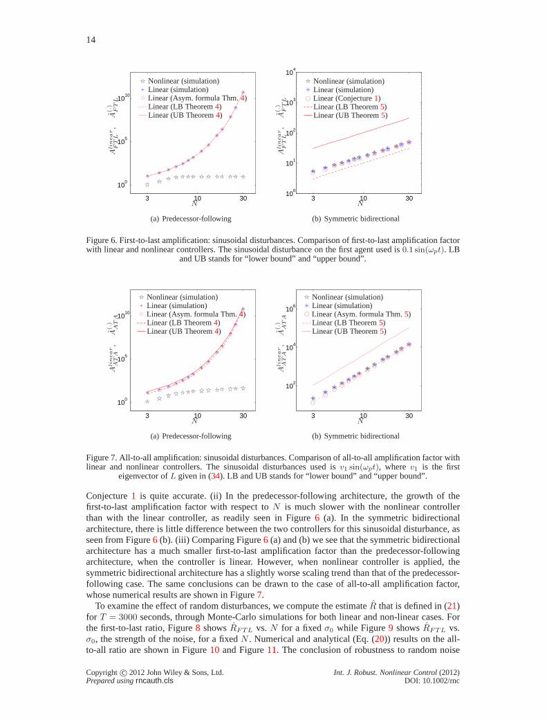
In this section, we present robustness metrics of the 1-D network with linear and nonlinearcontrollers empirically estimated using numerical computations. The analytical predictions of theperformance metrics for the linear controllers are also presented to verify these predictions. Thecontrollers used are the ones given by (13).

Figure 6 shows the first-to-last amplification factor as a function ofN : Figure 6 (a) is forpredecessor following and Figure6 (b) is for symmetric bidirectional. The following observationsare made. (i) The lower and upper bounds and asymptotic formulae derived are quite accurate,especially for the predecessor following case. For the symmetric bidirectional architecture,


14

3 10 30

100

105

1010

N

Ali

nea

rF

TL

,A

(.)

FT

L

Linear (simulation)Linear (Asym. formula Thm.4)

Nonlinear (simulation)

Linear (LB Theorem4)Linear (UB Theorem4)


3 10 3010

0

101

102

103

104

N

Ali

nea

rF

TL

,A

(.)

FT

L

Linear (simulation)Linear (Conjecture1)




Figure 6. First-to-last amplification: sinusoidal disturbances. Comparison of first-to-last amplification factorwith linear and nonlinear controllers. The sinusoidal disturbance on the first agent used is0.1 sin(ωpt). LB

and UB stands for “lower bound” and “upper bound”.

3 10 30

100

105

1010

N

Ali

nea

rA

TA

,A

(.)

AT

A





3 10 30

102

104

106

N

Ali

nea

rA

TA

,A

(.)

AT

A





Figure 7. All-to-all amplification: sinusoidal disturbances. Comparison of all-to-all amplification factor withlinear and nonlinear controllers. The sinusoidal disturbances used isv1 sin(ωpt), wherev1 is the first

eigenvector ofL given in (34). LB and UB stands for “lower bound” and “upper bound”.

Conjecture1 is quite accurate. (ii) In the predecessor-following architecture, the growth of thefirst-to-last amplification factor with respect toN is much slower with the nonlinear controllerthan with the linear controller, as readily seen in Figure6 (a). In the symmetric bidirectionalarchitecture, there is little difference between the two controllers for this sinusoidal disturbance, asseen from Figure6 (b). (iii) Comparing Figure6 (a) and (b) we see that the symmetric bidirectionalarchitecture has a much smaller first-to-last amplificationfactor than the predecessor-followingarchitecture, when the controller is linear. However, whennonlinear controller is applied, thesymmetric bidirectional architecture has a slightly worsescaling trend than that of the predecessor-following case. The same conclusions can be drawn to the caseof all-to-all amplification factor,whose numerical results are shown in Figure7.

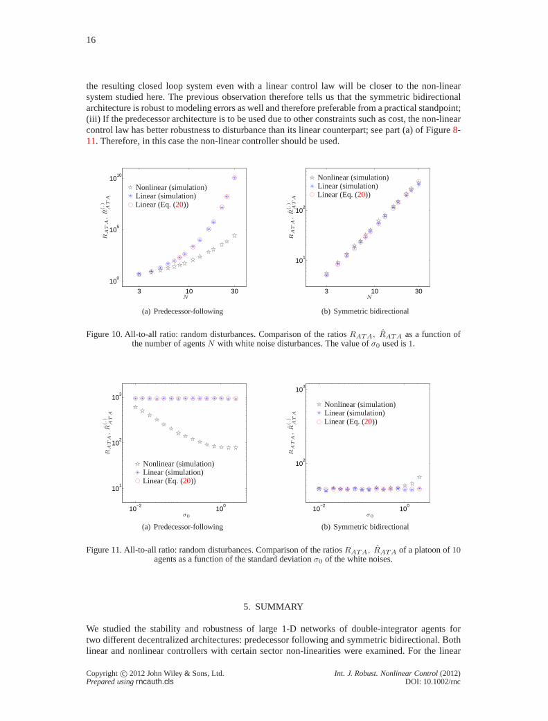
To examine the effect of random disturbances, we compute theestimateR that is defined in (21)for T = 3000 seconds, through Monte-Carlo simulations for both linear and non-linear cases. Forthe first-to-last ratio, Figure8 showsRFTL vs.N for a fixedσ0 while Figure9 showsRFTL vs.σ0, the strength of the noise, for a fixedN . Numerical and analytical (Eq. (20)) results on the all-to-all ratio are shown in Figure10 and Figure11. The conclusion of robustness to random noise


15

drain from Figure8-11 are the same as that for robustness to sinusoidal disturbances, we omit thediscussion due to space limit.

3 10 30

100

105

1010

N

RF

TL

,R

(.)

FT

L Linear (simulation)Nonlinear (simulation)

Linear (Eq. (20))


3 10 3010

−1

100

101

102

103

N

RF

TL

,R

(.)

FT


Linear (Eq. (20))


Figure 8. First-to-last ratio: random disturbance (σ0 = 1), for both linear and non-linear controllers.

10−2

100

101

102

103

σ0

RF

TL

,R

(.)

FT

L

Linear (simulation)Nonlinear (simulation)

Linear (Eq. (20))


10−2

100

100

101

102

σ0

RF

TL

,R

(.)

FT


Linear (Eq. (20))


Figure 9. First-to-last ratio: random disturbances. Comparison of the ratiosRFTL, RFTL of a network of10 agents as a function of the standard deviationσ0 of the white noises.

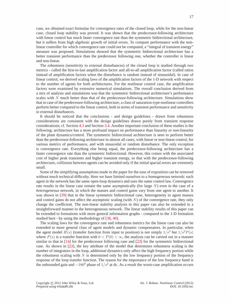
4.3. Design guidelines based on robustness

Based on the empirical as well as the analytical results, therobustness performance results aresummarized in TaleIII and TableIV. A few broad conclusions can be arrived at that are useful formaking design choices: (i) by comparing part (a) with part (b) for Figures8-11we conclude that thepredecessor following architecture has poorer performance compared to the symmetric bidirectionalone, and the difference gets more pronounced asN increases. Moreover, this conclusion holdsirrespective of whether the disturbance is sinusoidal or random, and whether the first-to-last ratioor the all-to-all ratio is used as a metric of robustness; (ii) If symmetric bidirectional architectureis indeed used, both the linear and non-linear control laws have almost identical robustness. Theonly exception is when the strength of the disturbance is large, in which case the non-linear controllaw performs poorly compared to the linear one. Thus, a designer can use the linear control lawdue to simplicity without losing performance. Since, actuator saturation will be present in practice,


16

the resulting closed loop system even with a linear control law will be closer to the non-linearsystem studied here. The previous observation therefore tells us that the symmetric bidirectionalarchitecture is robust to modeling errors as well and therefore preferable from a practical standpoint;(iii) If the predecessor architecture is to be used due to other constraints such as cost, the non-linearcontrol law has better robustness to disturbance than its linear counterpart; see part (a) of Figure8-11. Therefore, in this case the non-linear controller should be used.

3 10 30

100

105

1010

N

RA

TA

,R

(.)

AT

A Linear (simulation)Nonlinear (simulation)

Linear (Eq. (20))


3 10 30

101

102

NR

AT

A,

R(.)

AT

A


Linear (Eq. (20))


Figure 10. All-to-all ratio: random disturbances. Comparison of the ratiosRATA, RATA as a function ofthe number of agentsN with white noise disturbances. The value ofσ0 used is1.

10−2

100

101

102

103

σ0

RA

TA

,R

(.)

AT

A


Linear (Eq. (20))


10−2

100

102

103

σ0

RA

TA

,R

(.)

AT

A Linear (simulation)Nonlinear (simulation)

Linear (Eq. (20))


Figure 11. All-to-all ratio: random disturbances. Comparison of the ratiosRATA, RATA of a platoon of10agents as a function of the standard deviationσ0 of the white noises.

5. SUMMARY

We studied the stability and robustness of large 1-D networks of double-integrator agents fortwo different decentralized architectures: predecessor following and symmetric bidirectional. Bothlinear and nonlinear controllers with certain sector non-linearities were examined. For the linear


17

case, we obtained exact formulae for convergence rates of the closed loop, while for the non-linearcase, closed loop stability was proved. It was shown that thepredecessor-following architecturewith linear control has much faster convergence rate than the symmetric bidirectional architecture,but it suffers from high algebraic growth of initial errors.To compare performance with the non-linear controller for which convergence rate could not be computed, a “integral of transient energy”measure was proposed. Simulations showed that the symmetric bidirectional architecture has abetter transient performance than the predecessor following one, whether the controller is linearand non-linear.

The robustness (sensitivity to external disturbances) of the closed loop is studied through twometrics - called the first-to-last amplification factor and all-to-all amplification factor (called ratiosinstead of amplification factors when the disturbance is random instead of sinusoidal). In case oflinear control, we derived scaling laws of the amplificationfactors of the 1-D network with respectto the number of agents for both architectures. For the nonlinear control case, the amplificationfactors were examined by extensive numerical simulations.The overall conclusion derived froma mix of analysis and simulations was that the symmetric bidirectional architecture’s performancescales withN much better than that of the predecessor-following architecture. Simulations showthat in case of the predecessor-following architecture, a class of saturation-type nonlinear controllersperform better compared to the linear control, both in termsof transient performance and sensitivityto external disturbances.

It should be noticed that the conclusions - and design guidelines - drawn from robustnessconsiderations are consistent with the design guidelines drawn purely from transient responseconsiderations; cf. Section4.3and Section3.4. Another important conclusion of these studies is thefollowing: architecture has a more profound impact on performance than linearity or non-linearityof the plant dynamics/control. The symmetric bidirectional architecture is seen to perform betterthan the predecessor-following architecture in almost allcases, with linear or non-linear control, forvarious metrics of performance, and with sinusoidal or random disturbance. The only exceptionis convergence rate. Everything else being equal, the predecessor-following architecture has afaster convergence rate than the symmetric bidirectional.However, this comes with the associatedcost of higher peak transients and higher transient energy,so that with the predecessor-followingarchitecture, collisions between agents can be avoided only if the initial spacial errors are extremelysmall.

Some of the simplifying assumptions made in the paper for theease of exposition can be removedwithout much technical difficulty. Here we have limited ourselves to ahomogeneousnetwork: eachagent in the network has the same open-loop dynamics and usesthe same control law. Convergencerate results in the linear case remain the same asymptotically (for largeN ) even in the case of aheterogeneousnetwork, in which the masses and control gains vary from one agent to another. Itwas shown in [39] that in the linear symmetric bidirectional case, heterogeneity in agent massesand control gains do not affect the asymptotic scaling (withN ) of the convergence rate, they onlychange the coefficient. The non-linear stability analysis in this paper can also be extended in astraightforward manner to the heterogeneous network. The linear stability results of this paper canbe extended to formations with more general information graphs - compared to the 1-D formationstudied here - by using the methodology of [38, 40].

The scaling laws for the convergence rate and robustness metrics for the linear case can also beextended to more general class of agent models and dynamic compensators. In particular, whenthe agent modelH(s) (transfer function from input to position) is not simply1/s2 but 1/s2P (s)whereP (s) is a transfer function with0 < P (0) <∞, the analysis can be carried out in a mannersimilar to that in [14] for the predecessor following case and [23] for the symmetric bidirectionalcase. As shown in [23], the key attribute of the model that determines robustnessscaling is thenumber of integrators in the loop, additional dynamics onlyaffect the high frequency portion whilethe robustness scaling withN is determined only by the low frequency portion of the frequencyresponse of the loop transfer function. The reason for the importance of the low frequency band isthe unbounded gain and−1800 phase of1/s2 at dc. As a result the worst-case amplification occurs


18

at a progressively lower frequency asN increases. Recall Theorem5: the peak frequencies for thesymmetric bidirectional case isO(1/N).

It should be emphasized that the results for the symmetric architecture obtained here do notextend to theasymmetriccase, in which an agent uses information from its predecessor (front-neighbor) differently than the information from its follower (back neighbor). One can introducea mistuning parameterǫ ∈ [−1, 1] to quantity this asymmetry:ǫ = 0 corresponds to the case ofsymmetric bidirectional case whileǫ = 1 corresponds to the predecessor following architecture,with 0 < ǫ < 1 corresponding to a case when the front neighbor’s information is weighted moreheavily than that of the back neighbor, and−1 < ǫ < 0 corresponding to the opposite. The differencebetween the two architectures established here already provides evidence that asymmetry has a non-negligible effect. Recent works have shown that even small amount of asymmetry can have a hugeimpact, on both convergence rate [41, 39] and robustness in terms of, respectively,H∞ norm [28]andH2 norm [30]. It was shown in [39, 28, 30] that asymmetry can either significantly improveor deteriorate the system’s convergence rate and robustness, depends on the choice of asymmetry.These works have studied the linear case. Analysis of stability with general asymmetric non-linearcontrol is an open problem. In fact, analysis of the sensitivity to disturbance with general asymmetriccontrol (linear or non-linear) is also an open problem.

REFERENCES

1. Hedrick JK, Tomizuka M, Varaiya P. Control issues in automated highway systems.IEEE Control SystemsMagazineDecember 1994;14:21 – 32, doi:10.1109/37.334412.

2. Ioannou P.Automated Highway Systems. Plenum Pub Corp, 1997.3. Tanner H, Christodoulakis D. Decentralized cooperativecontrol of heterogeneous vehicle groups.Robotics and

autonomous systems2007;55(11):811–823.4. Hoffman T. GRAIL: Gravity mapping the moon.IEEE Aerospace conference, 2009; 1–8, doi:10.1109/AERO.2009.

4839327.5. Okubo A. Dynamical aspects of animal grouping: swarms, schools, flocks, and herds.Advances in Biophysics1986;

22:1–94.6. Ioannou P, Chien C. Autonomous intelligent cruise control. Vehicular Technology, IEEE Transactions on1993;

42(4):657–672.7. Ioannou P, Xu Z, Eckert S, Clemons D, Sieja T. Intelligent cruise control: theory and experiment.Decision and

Control, 1993., Proceedings of the 32nd IEEE Conference on, IEEE, 1993; 1885–1890.8. Bjornberg A. Autonomous intelligent cruise control.Vehicular Technology Conference, 1994 IEEE 44th, IEEE,

1994; 429–433.9. Darbha S, Rajagopal K. Intelligent cruise control systems and traffic flow stability.Transportation Research Part

C: Emerging Technologies1999;7(6):329–352.10. Darbha S, Hedrick JK. String stability of interconnected systems.IEEE Transactions on Automatic ControlMarch

1996;41(3):349–356.11. Darbha S, Hedrick J, Chien C, Ioannou P. A comparison of spacing and headway control laws for automatically

controlled vehicles.Vehicle System Dynamics1994;23(8):597–625.12. Zhang Y, Kosmatopoulos EB, Ioannou PA, Chien CC. Autonomous intelligent cruise control using front and back

information for tight vehicle following maneuvers.IEEE Transactions on Vehicular TechnologyJanuary 1999;48:319–328.

13. Klinge S, Middleton R. Time headway requirements for string stability of homogeneous linear unidirectionallyconnected systems.Proceedings of the 48th IEEE Conference on Decision and Control, IEEE, 2009; 1992–1997.

14. Seiler P, Pant A, Hedrick JK. Disturbance propagation invehicle strings.IEEE Transactions on Automatic ControlOctober 2004;49:1835–1841.

15. Lestas I, Vinnicombe G. Scalability in heterogeneous vehicle platoons.American Control Conference, 2007; 4678–4683.

16. Liu X, Goldsmith A, Mahal S, Hedrick J. Effects of communication delay on string stability in vehicle platoons.Intelligent Transportation Systems, 2001. Proceedings. 2001 IEEE, IEEE, 2001; 625–630.

17. Peppard L. String stability of relative-motion PID vehicle control systems.Automatic Control, IEEE Transactionson1974;19(5):579–581.

18. Chu K. Decentralized control of high-speed vehicular strings.Transportation Science1974;8(4):361.19. Stotsky A, Chien C, Ioannou P. Robust platoon-stable controller design for autonomous intelligent vehicles.

Proceedings of the 33rd IEEE Conference on Decision and Control, vol. 3, IEEE, 1994; 2431–2436.20. Bose A, Ioannou P. Environmental evaluation of intelligent cruise control (icc) vehicles.Intelligent Transportation

Systems, 2000. Proceedings. 2000 IEEE, IEEE, 2000; 352–357.21. Middleton R, Braslavsky J. String instability in classes of linear time invariant formation control with limited

communication range.IEEE Transactions on Automatic Control2010;55(7):1519–1530.22. Khatir ME, Davison EJ. Decentralized control of a large platoon of vehicles using non-identical controllers.

Proceedings of the 2004 American Control Conference, 2004; 2769–2776.


19

23. Barooah P, Hespanha J. Error amplification and disturbance propagation in vehicle strings with decentralized linearcontrol.44th IEEE Conference on Decision and Control, IEEE, 2005; 4964 – 4969.

24. Jovanovic MR, Bamieh B. On the ill-posedness of certainvehicular platoon control problems.IEEE Trans.Automatic ControlSeptember 2005;50(9):1307–1321.

25. Munz U, Papachristodoulou A, Allgower F. Robust Consensus Controller Design for Nonlinear Relative DegreeTwo Multi-Agent Systems With Communication Constraints.Automatic Control, IEEE Transactions on2011;56(1):145–151.

26. Yadlapalli SK, Darbha S, Rajagopal KR. Information flow and its relation to stability of the motion of vehicles in arigid formation.IEEE Transactions on Automatic ControlAugust 2006;51(8).

27. Darbha S, Pagilla PR. Limitations of employing undirected information flow graphs for the maintenance of rigidformations for heterogeneous vehicles.International journal of engineering science2010;48(11):1164–1178.

28. Veerman J. Stability of large flocks: an example July 2009. arXiv:1002.0768.29. Bamieh B, Jovanovic M, Mitra P, Patterson S. Coherence inlarge-scale networks: Dimension depen-

dent limitations of local feedback.IEEE Transactions on Automatic Control, in press,2012; URLhttp://arxiv.org/abs/1112.4011v1.

30. Lin F, Fardad M, Jovanovic M. Optimal control of vehicular formations with nearest neighbor interactions.IEEETransactions on Automatic Control, in press,2012; URLhttp://arxiv.org/abs/1112.4113v1.

31. Stankovic S, Stanojevic M, Siljak D. Decentralized overlapping control of a platoon of vehicles.Control SystemsTechnology, IEEE Transactions on2000;8(5):816–832.

32. Jovanovic M, Fowler J, Bamieh B, D’Andrea R. On avoiding saturation in the control of vehicular platoons.Proc.American Control Conference, vol. 3, 2004; 2257–2262.

33. Warnick S, Rodriguez A. Longitudinal control of a platoon of vehicles with multiple saturating nonlinearities.American Control Conference, vol. 1, IEEE, 1994; 403–407.

34. Khalil H.Nonlinear Systems 3rd. Prentice hall Englewood Cliffs, NJ, 2002.35. Simon D.Optimal state estimation: Kalman, H [infinity] and nonlinear approaches. John Wiley and Sons, 2006.36. Bamieh B, Dahleh M. Exact computation of traces and h2 norms for a class of infinite-dimensional problems.

Automatic Control, IEEE Transactions on2003;48(4):646–649.37. Higham D. An algorithmic introduction to numerical simulation of stochastic differential equations.SIAM review

2001;43(3):525–546.38. Hao H, Barooah P. Decentralized control of large vehicular formations: stability margin and sensitivity to external

disturbances.Arxiv preprint arXiv:1108.14092011; URLhttp://arxiv.org/abs/1108.1409 .39. Hao H, Barooah P. Control of large 1D networks of double integrator agents: role of heterogeneity and

asymmetry on stability margin.IEEE Conference on Decision and Control, 2010; 7395 – 7400. Expanded version:arXiv:1011.0791.

40. Hao H, Barooah P, Mehta PG. Stability margin scaling of distributed formation control as a function of networkstructure.IEEE Transactions on Automatic ControlApril 2011; 56(4):923–929.

41. Hao H, Barooah P. On achieving size-independent stability margin of vehicular lattice formations with distributedcontrol.To appear in IEEE Transactions on Automatic Control,October 2012; Expanded version: arXiv:1108.1844.

42. Hao H, Barooah P, Veerman J. Effect of network structure on the stability margin of large vehicle formation withdistributed control.Proceedings of the 49th IEEE conference on Decision and Control, 2010.

43. Yueh W, Cheng S. Explicit eigenvalues and inverses of tridiagonal toeplitz matrices with four perturbed corners.The Australian & New Zealand Industrial and Applied Mathematics (Anziam) Journal2008;49(3):361–388.

44. Haberman R.Elementary applied partial differential equations: with Fourier series and boundary value problems.Prentice-Hall, 2003.

APPENDIX

Proof of Theorem1. For the predecessor-following architecture with linear controller, it followsfrom straightforward algebra that the state matrixA can be written as

A =

A1

A2 A1

.. .. ..A2 A1

, A1 =

[

0 1−k0 −b0

]

, A2 =

[

0 0k0 b0

]

. (24)

The state matrixA is a lower block triangular matrix, whose eigenvalues are determined by the block

matrixA1 on the diagonal. The eigenvalues ofA1 are−b0±

√b20−4k0

2 . Since there areN such blockmatrices on the diagonal ofA, its eigenvalues have multiplicityN . Since the least stable eigenvalue

is the one closest to the imaginary axis, it is given byµ1 =−b0+

√b20−4k0

2 , and this eigenvalue occurswith multiplicity N .The result for the symmetric bidirectional architecture follows from Theorem4 in [42] in astraightforward manner and is therefore omitted.

The proof of Theorem2 will use the following proposition.


http://arxiv.org/abs/1112.4011v1

http://arxiv.org/abs/1112.4113v1

http://arxiv.org/abs/1108.1409

20

Proposition 1Consider the second order autonomous systemy1 = y2, y2 = −f(y1 − u1) − g(y2 − u2), wherey1, y2, u1, u2 ∈ R and the odd functionsf, g : R → R lie in the sectorsf ∈ [ε1,K1], g ∈ [ε2,K2],where 0 < ε1 ≤ K1 <∞, 0 < ε2 ≤ K2 <∞. The origin of the unforced system (withu(t) =[u1(t), u2(t)]

T ≡ 0) is globally exponentially stable (GES) and the system is input-to-state stable(ISS) withu as the input. 2

Proof of Proposition1. First, we consider the unforced system with statey = [y1, y2]T ,

y1 = y2, y2 = −f(y1) − g(y2). (25)

Consider the following Lyapunov function candidate:

V (y) =1

2yTPy + γ

∫ y1

0

f(z)dz, (26)

whereP =

[

1 11 γ

]

and γ ≥ max {1, 1ε2

+ (1+K2)2

ε1ε2}, which ensures thatP is positive definite.

From the Rayleigh Ritz Theorem [34], we have the following inequalityλmin(P )‖y‖2 ≤ yTPy ≤λmax(P )‖y‖2, whereλmin(P ) > 0, λmax(P ) > 0 are the minimum and maximum eigenvalues ofPrespectively. This shows thatV (y) is radially unbounded, and in addition satisfies the following

V (y) ≤ λmax(P )

2‖y‖2 +

γK1

2y21 ≤ λmax(P ) + γK1

2‖y‖2, (27)

where the second inequality follows from the fact that the function f(z) belongs to the sector[ε1,K1]. The derivative ofV along the trajectory of (25) is given by

V = yTP y + γf(y1)y2 = −y1f(y1) − γy2g(y2) + y22 + y1y2 − y1g(y2)

≤ −ε1y21 − (γε2 − 1)y2

2 + (1 +K2)|y1||y2|,

≤ −1

2(ε1y

21 + (γε2 − 1)y2

2) −1

2[ε1y

21 − 2(1 +K2)|y1||y2| + (γε2 − 1)y2

2)]

≤ −1

2(ε1y

21 + (γε2 − 1)y2

2) ≤ −1

2min{ε1, (γε2 − 1)}‖y‖2, (28)

where the second last inequality follows fromγ ≥ max {1, 1ε2

+ (1+K2)2

ε1ε2}, upon a completion of

squares. SinceV is radially unbounded and satisfies (27), it follows from (28) that the originy = 0of (25) is globally exponentially stable. Since the functionsf, g are assumed to be smooth enough,the ISS property follows from the fact that a globally exponentially stable system with inputu isISS [34, Lemma 4.6].

Proof of Theorem2. We first consider the subsystem consisted of only the first agent. Its closed-loop dynamics can be written as below by using the factp0 = ˙p0 ≡ 0,

¨p1 = −f(p1 − p0) − g( ˙p1 − ˙p0) ⇒ ¨p1 = −f(p1) − g( ˙p1) ⇒ x(1) = f1(x(1)),

wherex(1) = [p1, ˙p1]T . From Proposition1, we have that the originx(1) = 0 of the subsystem

x(1) = f1(x(1)) is GES. Next, we consider the subsystem consisted of the firsttwo agents. Its closed-

loop dynamics can be written as

{

¨p1 = −f(p1) − g( ˙p1),¨p2 = −f(p2 − p1) − g( ˙p2 − ˙p1),

⇒ x(1+2) = f1+2(x(1+2)),


21

wherex(1+2) = [p1, ˙p1, p2, ˙p2]T . The above dynamics can be divided into two parts:

x(1+2) = f1+2(x(1+2)) ⇒

{

x(1) = f1(x(1)),

x(2) = f2(x(2), x(1)),

(29)

wherex(2) = [p2, ˙p2]T . The unforced systemx(2) = f2(x

(2), 0) is given by

x(2) = f1(x(2), 0) ⇒ ¨p2 = −f(p2) − g( ˙p2).

According to Proposition1, the originx(2) = 0 of the unforced systemx(2) = f2(x(2), 0) is GES

and it’s ISS withx(1) as the input. We now invoke [34, Lemma 4.7], the origin of the cascadesystemx(1+2) = f1+2(x

(1+2)) given in (29) is globally asymptotically stable (GAS). We now provethe origin of the whole system is GAS by induction. Suppose the originx(1+···+N−1) = 0 of thesubsystem consisted of the firstN − 1 agentsx(1+···+N−1) = f1+···+N−1(x

(1+···+N−1)) is GAS,we consider the whole system, whose dynamics is given by

x = f(x) ⇒ x(1+···+N) = f1+···+N (x(1+···+N)).

The above dynamics can be divided into two parts:

x(1+···+N) = f1+···+N (x(1+···+N)), ⇒{

x(1+···+N−1) = f1+···+N−1(x(1+···+N−1)),

x(N) = fN (x(N), x(1+···+N−1)),(30)

The unforced systemx(N) = fN (x(N), 0) is given by

x(N) = fN (x(N), 0) ⇒ ¨pN = −f(pN) − g( ˙pN ).

According to Proposition1, the originx(N) = 0 of the unforced systemx(N) = fN (x(N), 0) is GESand it’s ISS withx(1+···+N−1) as the input. Invoking [34, Lemma 4.7] again, we see that the originx = x(1+···+N) = 0 of the whole system whose dynamics is given in (30) is globally asymptoticallystable. This completes the proof by induction.

Proof of Theorem3. For the 1-D network of double-integrator agents with symmetric bidirectionalarchitecture, we consider the following Lyapunov functioncandidate, which is inspired by the oneused in [25]:

V (x) =

N∑

i=1

∫ pi−pi−1

0

f(z)dz +1

2

N∑

i=1

˙p2i ,

wherex = [p1, ˙p1, p2, ˙p2, · · · , pN , ˙pN ]. The derivative ofV along the trajectory of (7) with wi = 0is

V =

N∑

i=1

f(pi − pi−1)( ˙pi − ˙pi−1) +

N∑

i=1

˙pi¨pi = −

N∑

i=1

( ˙pi − ˙pi−1)g( ˙pi − ˙pi−1) ≤ 0,

If V = 0, then we have˙pi = 0 for all i, sinceg(z) satisfieszg(z) > 0, ∀x 6= 0 and ˙p0 = 0 bydefinition. Asymptotic stability now follows from LaSalle’s Invariance Principle. In addition, wehaveV (x) → ∞ as‖x‖ → ∞. Therefore, the Lyapunov functionV is radially unbounded, and weget global asymptotic stability.


22

Proof of Theorem5. Take Laplace transform of the coupled-ODE model (7) and assume zeroinitial conditions, the transfer function from the disturbancew = [w1, . . . , wN ]T to position errorp = [p1, . . . , pN ]T is given by

G(s) = (s2I + (b0s+ k0)L)−1, (31)

whereI is theN ×N identity matrix andL is given by

L =

2 −1−1 2 −1

. ... ..

. ..−1 2 −1

−1 1

. (32)

Following Theorem 3.1 of [43], the eigenvalues ofL and its corresponding orthonormal eigenvectorsare given by

λℓ = 2 − 2 cos((2ℓ− 1)π

2N + 1) = 4 sin2(

(2ℓ− 1)π

2(2N + 1)), (33)

vℓ =2√

2N + 1

[

sin((2ℓ− 1)π

2N + 1), · · · , sin(

(2ℓ− 1)Nπ

2N + 1)]T. (34)

(1) For the case of first-to-last amplification, the transfer functionGFTL from disturbancew1 onthe first agent to the position error of the last agentpN isGFTL = φT

NG(s)φ1, whereφi is thei-thcanonical basis vector ofR

N whosei-th entry is1 and the rest are all0’s. Therefore,

GFTL(s) =φTNM(s2I + (b0s+ k0)Λ)−1MTφ1

=φTNM

1s2+λ1b0s+λ1k0

.. .1

s2+λN b0s+λN k0

MTφ1

=4

2N + 1

N∑

ℓ=1

(

sin(2ℓ− 1)Nπ

2N + 1sin

(2ℓ− 1)π

2N + 1Gℓ(s)

)

, (35)

whereM = [v1, v2, · · · , vN ], Λ = diag(λ1, λ2, · · · , λN ) such thatL = MΛMT and

Gℓ(s) :=1

s2 + λℓb0s+ λℓk0. (36)

It can be shown using straightforward calculus that for eacheigenvalueλℓ, the maximum amplitudeand its peak frequency ofGℓ(s) are

Aℓ := maxω

|Gℓ(jω)| =

{

2

λ3/2ℓ b0

√4k0−λℓb20

, if λℓ ≤ 2k0/b20,

1λℓk0

, otherwise.(37)

ωℓ := argmax |Gℓ(jω)| =

{√

4λℓk0−2λ2ℓb20

2 , if λℓ ≤ 2k0/b20,

0, otherwise.(38)

From (33), λ1 < λ2 < · · · < λN , which can be used to show by straightforward algebra thatA1 > A2 > · · · > AN . For future use, we have from2π θ ≤ sin θ ≤ θ, ∀ θ ∈ [0, π

2 ] that

4(2ℓ− 1)2

(2N + 1)2≤ λℓ ≤

(2ℓ− 1)2π2

(2N + 1)2. (39)


23

We first expressGFTL(s) in (35) as

GFTL(s) = T (s) + Z(s), (40)

where

T (s) =4

2N + 1sin

Nπ

2N + 1sin

π

2N + 1G1(s), (41)

Z(s) =4

2N + 1

N∑

ℓ=2

(

sin(2ℓ− 1)Nπ

2N + 1sin

(2ℓ− 1)π

2N + 1Gℓ(s)

)

. (42)

Now,

supω

|GFTL(jω)| ≤ supω

|T (jω)| + supω

|Z(jω)| = |T (jω1)| + supω

|Z(jω)|,

supω

|GFTL(jω)| ≥ |T (jω1) + Z(jω1)| ≥ |T (jω1)| − |Z(jω1)|,

whereω1 is given in (38). Combining the above two inequalities, we obtain

|T (jω1)| − |Z(jω1)| ≤ supω

|G(jω)| ≤ |T (jω1)| + supω

|Z(jω)|. (43)

We now derive a upper bound forsupω |Z(jω)|. Using triangle inequality, it follows from (42)satisfies

supω

|Z(jω)| ≤ 4

2N + 1

N∑

ℓ=2

(

sin(2ℓ− 1)Nπ

2N + 1sin

(2ℓ− 1)π

2N + 1sup

ω|Gℓ(jω)|

)

≤ 4

2N + 1

N∑

ℓ=2

(

sin(2ℓ− 1)π

2N + 1Aℓ

)

≤ 4

2N + 1

N∑

ℓ=2

(2ℓ− 1)π

2N + 1Aℓ, (44)

where the last inequality follows from the fact thatsin θ ≤ θ for θ ∈ [0, π/2] and (2ℓ−1)π2N+1 ∈ [0, π/2]

for 2 ≤ ℓ ≤ N . From Eq. (37), we notice that depending on whetherλℓ ≤ 2k0/b20 or not, the

expressions ofAℓ’s are different. First we have

λℓ ≤ 2k0/b20 ⇒ 1

4k0 − λℓb20≤ 1

2k0, and λℓ > 2k0/b

20 ⇒ 1

λℓ<

b202k0

. (45)

Let Nc be in the index so thatℓ ≤ Nc ⇒ λℓ ≤ 2k0/b20 andℓ > Nc ⇒ λℓ > 2k0/b

20. The inequality

in (44) can be written as

supω

|Z(jω)| ≤ 4

2N + 1

(

Nc∑

ℓ=2

(2ℓ− 1)π

2N + 1

2

λ3/2ℓ b0

√

4k0 − λℓb20+

N∑

ℓ=Nc

(2ℓ− 1)π

2N + 1

1

λℓk0

)

≤ 4

(2N + 1)2

N∑

ℓ=2

((2ℓ− 1)π√2k0b0

2

λ3/2ℓ

+ (2ℓ− 1)πb202k2

0

)

. (46)

From (39), we have 1

λ3/2ℓ

≤ (2N+1)3

8(2ℓ−1)3 . The inequality (46) becomes

supω

|Z(jω)| ≤ π(2N + 1)√2k0b0

N∑

ℓ=2

1

(2ℓ− 1)2+

2b20π

k20(2N + 1)2

N∑

ℓ=2

(2ℓ− 1)

≤ π(2N + 1)

4√

2k0b0

∞∑

ℓ=2

1

(ℓ − 1)2+

2b20π

k20(2N + 1)2

N∑

ℓ=2

(2ℓ− 1)

≤ π(2N + 1)

4√

2k0b0(π2

6− 1) +

2b20π

k20(2N + 1)2

(N2 − 1), (47)


24

where the last inequality follows from∑∞

ℓ=11ℓ2 = π2

6 and∑N

ℓ=1 (2ℓ− 1) = N2. This proves anupper bound forsupω |Z(jω)|.We now obtain an upper bound for|T (jω1)|

|T (jω1)| =4

2N + 1sin

Nπ

2N + 1sin

π

2N + 1A1 ≤ 4

2N + 1

π

2N + 1A1

≤ 4

2N + 1

π

2N + 1

2

λ3/21 b0

√

4k0 − λ1b20+

4

2N + 1

π

2N + 1

1

λ1k0

≤ 4π

(2N + 1)2(2N + 1)3

4b0√

2k0

+4π

(2N + 1)2b202k2

0

≤ π(2N + 1)

b0√

2k0

+2b20π

k20(2N + 1)2

, (48)

Substituting inequalities (47) and (48) into (43), we get a upper bound forsupω |GFTL(jω)|

supω

|GFTL(jω)| ≤( π3 + 18π

12b0√

2k0

)

N + c1, (49)

wherec1 is a constant independent ofN .To prove the lower bound for|T (jω1)|, we first use the fact that2π θ ≤ sin θ, ∀ θ ∈ [0, π

2 ],

|T (jω1)| =4

2N + 1sin

Nπ

2N + 1sin

π

2N + 1A1

≥ 4

2N + 1

2

π

Nπ

2N + 1

2

π

π

2N + 1A1 ≥ 16N

(2N + 1)3A1. (50)

For any fixedk0, b0, whenN is large, we haveλ1 < 2k0/b20, which implies

A1 =2

λ3/21 b0

√

4k0 − λ1b20≥ 1

λ3/21 b0

√k0

≥ 1

b0√k0

(2N + 1)3

π3, (51)

where the last inequality is obtained from (39). The inequality (50) now becomes

|T (jω1)| ≥16N

π3b0√k0

. (52)

In addition, we have

|Z(jω1)| ≤4

2N + 1

N∑

ℓ=2

((2ℓ− 1)π

2N + 1|Gℓ(jω1)|

)

≤ 4

2N + 1

N∑

ℓ=2

((2ℓ− 1)π

2N + 1

1

λℓk0

√

(1 − λ1/λ2)2

)

.

From (39), we obtain that1λℓ≤ (2N+1)2

4(2ℓ−1)2 ,λ1

λ2≤ π2

36 . Thus the above inequality can be simplified to

|Z(jω1)| ≤ 2c2

N∑

ℓ=2

( (2ℓ− 1)

(2N + 1)2(2N + 1)2

4(2ℓ− 1)2

)

≤ 2c2

N∑

ℓ=2

( 1

(2ℓ− 1)

)

≤ c2

N−1∑

ℓ=1

1

ℓ,

wherec2 = π

2k0

√(1−π2/36)2

is a constant independent ofN . Moreover,∑N−1

ℓ=11ℓ = 1 +

∑N−1ℓ=2

1ℓ ≤

1 +∫ N−1

11s ds, we have

∑N−1ℓ=1

1ℓ ≤ 1 + ln(N − 1). Thus, we have

|Z(jω1)| ≤ c2 ln(N − 1) + c2. (53)

Substituting inequalities (53) and (52) into (43), we get a lower bound forsupω |GFTL(jω)|

supω

|GFTL(jω)| ≥ 16N

π3b0√k0

− c2 ln(N − 1) − c2. (54)


25

In addition, whenN is large, the constantsc1, c2 and theO(ln(N − 1)) term are dominated by theO(N) term, therefore we ignore them in (49) and (54) respectively, we obtain

( 16

π3b0√k0

)

N ≤ AlinearFTL ≤

( π3 + 18π

12b0√

2k0

)

N.

(2) For the case of all-to-all amplification, the transfer function from the disturbancew =[w1, · · · , wn] on all the agents to their position tracking errorsp = [p1, · · · , pN ] are given by

GATA(s) = G(s) = (s2I + (b0s+ k0)L)−1 = M(s2I + (b0s+ k0)Λ)−1MT

= M

G1(s). . .

GN (s)

MT , (55)

whereGℓ(s) is given in (36) andM is the orthonormal matrix given as before. TheH∞ norm ofGATA(s) (i.e.Alinear

ATA ) is now given by

‖GATA‖H∞=sup

ω‖GATA(jω)‖2 = sup

ω

√

λmax(G∗ATA(jω)GATA(jω))

= supω

maxℓ

1√

(−ω2 + λℓk0)2 + b20ω2λ2

ℓ

= maxω

maxℓ

‖Gℓ(jω)‖ = maxℓAℓ = A1,

whereA1 is given in (37). Again for largeN , we obtain from (51),

A1 ≥ 1

b0√k0

(2N + 1)3

π3. (56)

In addition, usingλ1 < 2k0/b20 and 1

λ3/2ℓ

≤ (2N+1)3

8 , we have

A1 =2

λ3/21 b0

√

4k0 − λ1b20≤ 2

λ3/21 b0

√2k0

≤ (2N + 1)3

4b0√

2k0

. (57)

Combining (56) and (57), we obtain

( 1

b0√k0π3

)

(2N + 1)3 ≤ AlinearATA ≤

( 1

4b0√

2k0

)

(2N + 1)3, ∀ N.

To get the asymptotic formula, whenN is large, we use the approximationλ1 ≈ π2

4N2 . Therefore,λ1 < 2k0/b

20 is true for large enoughN irrespective of the values ofk0 and b0. Substituting

λ1 ≈ π2

4N2 into (37) and (38), we obtain thatA1 ≈ 8N3√

k0b0π3 , ωp = ω1 ≈√

k0π2N . SinceAlinear

ATA = A1,this concludes the proof.

Proof of Corollary1. We first rewrite the coupled-ODE model (7) with linear controller as

¨p+ b0L ˙p+ k0Lp = v1 sin(ω1t), (58)

whereL is given in (32) andv1 is the eigenvector ofL corresponding to the smallest eigenvalueλ1

given in (34). By the method of eigenfunction expansion [44], we can writep(t) =∑N

ℓ=1 vℓhℓ(t),wherevℓ’s are the eigenvectors ofL given in (34). Substituting it into Eq. (58), we obtain

N∑

ℓ=1

(vℓhℓ(t) + b0Lvℓhℓ(t) + k0Lvℓhℓ(t)) = v1 sin(ω1t).


26

Due to superposition property of linear system, the above equation can be split intoN ordinarydifferential equations by usingLvℓ = λℓvℓ,

h1(t) + b0λℓh1(t) + k0λℓh1(t) = sin(ω1t),

hℓ(t) + b0λℓhℓ(t) + k0λℓhℓ(t) = 0, ℓ ∈ {2, · · · , N}.

Following straightforward algebra, the steady-state response of eachhℓ(t) is given by

h1(t) = A1 sin(ω1t+ ψ1), hℓ(t) = 0, ℓ ∈ {2, · · · , N},

whereA1 is given in (37). Thus the steady state response ofp is given byp = v1A1 sin(ω1t+ ψ1),which yields ‖p‖L2

‖w‖L2= A1. Recall from Theorem5 thatAlinear

ATA = A1, we complete the proof.

A “proof” of the conjecture is as follows. First notice that

AlinearFTL = sup

ω|GFTL(jω)| ≤ sup

ω|T (jω)| + sup

ω|Z(jω)| = |T (jω1)| + sup

ω|Z(jω)|

WhenN is large, the smallest eigenvalueλ1 ≈ π2

4N2 andsin Nπ2N+1 ≈ 1. The expression|T (jω1)| are

then approximately given by

|T (jω1)| ≈4

2N + 1

π

2N + 1A1 ≈ 4

2N + 1

π

2N + 1

(2N + 1)3

b0√k0π3

≈ 8N√k0b0π2

. (59)

Under the assumptionN is large, theO(N) term in the upper bound ofsupω |Z(jω)| which is givenin (47) dominates theO(1) term. Moreover, thisO(N) term is still smaller than|T (jω1)| givenin (59). Notice that this upper bound is obtained by letting each term in |Z(jω)| containingGℓ(jω)(ℓ ∈ {1, 2, · · · , N}) to achieve their maximum. In fact, the maximum of|GFTL(jω)| can be onlyachieved at a single frequency. We thus conjecture that thisfrequency should be equal toω1, the peakfrequency corresponding to the principal modelλ1. This idea is similar to that a wave equation’sresonance is achieved at the peak frequency correspond to its principle mode [44] and itsH∞ normis determined by the peak response of the principle mode. Now, theH∞ norm ofGFTL(s) is givenby ‖GFTL(jω)‖ = |G(jω1)|. Thus from (40), we have

|T (jω1)| − |Z(jω1)| ≤ supω

|G(jω)| ≤ |T (jω1)| + |Z(jω1)|

WhenN ≫ 1, the lower and upper bound will be dominated by the term|T (jω1)|, since|Z(jω1)|isO(ln(N − 1)) but |T (jω1)| isO(N). Thus theH∞ norm ofGFTL(s) is determined by|T (jω1)|.From (59), we have the firs-to-last amplificationAlinear

FTL ≈ |T (jω1)| = 8N√k0b0π2 .


stability and robustness of large platoons of …plaza.ufl.edu/hehao/papers/rnc.pdfacting on all the...

Documents