state of california department of transportation … · prepared in cooperation with the state of...

STATE OF CALIFORNIA DEPARTMENT OF TRANSPORTATION TECHNICAL REPORT DOCUMENTATION PAGE TR0003 (REV. 10/98)

1. REPORT NUMBER

CA14-2418 2. GOVERNMENT ASSOCIATION NUMBER

3. RECIPIENT’S CATALOG NUMBER

4. TITLE AND SUBTITLE

Comparative Study of Model Predictions and Data from Caltrans/CSMIP Bridge Instrumentation Program: A Case study on the Eureka-Samoa Channel Bridge

5. REPORT DATE

March 10, 2014 6. PERFORMING ORGANIZATION CODE

UCLA 7. AUTHOR(S)

Ertugrul Taciroglu, Anoosh Shamsabadi, Fariba Abazarsa, Robert L. Nigbor and S. Farid Ghahari

8. PERFORMING ORGANIZATION REPORT NO.

UCLA SGEL 2014-01, CA14-2418

9. PERFORMING ORGANIZATION NAME AND ADDRESS

Department of Civil and Environmental Engineering University of California, Los Angeles UCLA, 5731E Boelter Hall Los Angeles, CA 90095-1593

10. WORK UNIT NUMBER

11. CONTRACT OR GRANT NUMBER

65A0450

12. SPONSORING AGENCY AND ADDRESS

California Department of Transportation Engineering Service Center 1801 30th Street, MS 9-2/5i Sacramento, California 95816 California Department of Transportation Division of Research, Innovation, and System Information, MS-83P.O. Box 942873Sacramento, CA 94273-0001

13. TYPE OF REPORT AND PERIOD COVERED

Final Report 6/25/2012 – 11/01/2013

14. SPONSORING AGENCY CODE

913

15. SUPPLEMENTAL NOTES

Prepared in cooperation with the State of California Department of Transportation. 16. ABSTRACT

Long-span bridges provide vital transportation links to metropolitan regions, and their damage during earthquakes will cause significant hardship. Recognizing their importance, Caltrans and California Geological Survey have been deploying strong motion instrumentation on these structures for the last 25 years. In the present study, existing gaps between responses predicted using numerical models and real-life data are investigated through system identification and finite element model updating techniques for the Samoa Channel Bridge, which is located in Humboldt County, California. This study shows that seismic response of this bridge is different from its operational response, and the discrepancy increases with the shaking intensity. Also, while existing reduced-order numerical models of soil-pile interaction are observed to work well, they should be calibrated for specific vibration amplitudes.

17. KEY WORDS

Samoa Bridge, Modal Identification, Finite Element Model Updating

18. DISTRIBUTION STATEMENT

No restrictions. This document is available to the public through the National Technical Information Service, Springfield, VA, 22161

19. SECURITY CLASSIFICATION (of this report)

Unclassified 20. NUMBER OF PAGES

163 21. PRICE

Reproduction of completed page authorized

ADA Notice For individuals with sensory disabilities, this document is available in alternate formats. For alternate format information, contact the Forms Management Unit at (916) 445-1233, TTY 711, or write to Records and Forms Management, 1120 N Street, MS-89, Sacramento, CA 95814.

DISCLAIMER STATEMENT

This document is disseminated in the interest of information exchange. The contents of this

report reflect the views of the authors who are responsible for the facts and accuracy of the data

presented herein. The contents do not necessarily reflect the official views or policies of the State

of California or the Federal Highway Administration. This publication does not constitute a

standard, specification or regulation. This report does not constitute an endorsement by the

Department of any product described herein.

For individuals with sensory disabilities, this document is available in alternate formats. For

information, call (916) 654-8899, TTY 711, or write to California Department of Transportation,

Division of Research, Innovation and System Information, MS-83, P.O. Box 942873,

Sacramento, CA 94273-0001.

i

Comparative Study of Model Predictions and Data from the Caltrans-CGS Bridge Instrumentation Program: A Case study on the Eureka-Samoa

Channel Bridge

Ertugrul Taciroglu

Anoosh Shamsabadi

Fariba Abazarsa

Robert L. Nigbor

S. Farid Ghahari

University of California, Los Angeles

Department of Civil & Environmental Engineering

UCLA - SGEL

Report 2014-01

Structural & Geotechnical Engineering Laboratory

ii

Comparative Study of Model Predictions and Data from Caltrans-CGS Bridge Instrumentation

Program: A Case study on the Eureka-Samoa Channel Bridge

PRINCIPAL INVESTIGATOR

Ertugrul Taciroglu


CALTRANS COLLABORATOR

Anoosh Shamsabadi

California Department of Transportation

RESEARCH SCHOLAR

Fariba Abazarsa


CO-PRINCIPAL INVESTIGATOR

Robert L. Nigbor


POST-DOCTORAL RESEARCH ASSOCIATE

S. Farid Ghahari


Final Report No. CA14-2418

Final Report submitted to the California Department of Transportation (Caltrans) under Contract No. 65A0450

Department of Civil and Environmental Engineering


March 2014

iii

FUNDING AGENCY ACKNOWLEDGMENT

Support for this research was provided by the California Department of Transportation under Research Contract No. 65A0450 (and amendments thereto), which is gratefully acknowledged. Caltrans Research Project Manager Peter Lee is recognized for his assistance in contract administration. Authors also would like to thank Pat Hipley (Caltrans), Tony Shakal, Carl Petersen (California Geological Survey), Martin Turek, Carlos Ventura, Jason Dowling, Sheri Molnar, Yavuz Kaya (University of British Columbia) and other Caltrans personnel who participated in the planning and execution of the ambient vibration survey of the Samoa Channel Bridge in June 2013. Finally, authors would like to acknowledge Tom Ostrom, Chief of Caltrans Office of Earthquake Engineering, for his guidance and stewardship throughout the entire project.

DISCLAIMER STATEMENT

This document is disseminated in the interest of information exchange. The contents of this report reflect the views of the authors who are responsible for the facts and accuracy of the data presented herein. The contents do not necessarily reflect the official views or policies of the State of California or the Federal Highway Administration. This publication does not constitute a standard, specification or regulation. This report does not constitute an endorsement by the Department of any product described herein.

For individuals with sensory disabilities, this document is available in Braille, large print, audiocassette, or compact disk. To obtain a copy of this document in one of these alternate formats, please contact: the Division of Research and Innovation, MS-83, California Department of Transportation, P.O. Box 942873, Sacramento, CA 94273-0001.

iv

EXECUTIVE SUMMARY

This report presents results of a comprehensive study on the dynamic behavior and seismic responses of the main channel-crossing segment of the Eureka-Samoa Channel Bridge (a.k.a., the Humboldt Bay Bridge) located near the town of Eureka, California. Caltrans granted this study to a UCLA team led by Professor Ertugrul Taciroglu under contract no. 65A0450. The primary objective has been to develop quantitative comparisons of dynamic responses predicted through the use of high-fidelity state-of-the-art bridge models and real life data obtained through the Caltrans-CGS Bridge Instrumentation Program. Samoa Bridge was chosen specifically because it features a “free-field” station, a nearby geotechnical downhole array, an instrumented pile foundation, and seven significant earthquake events recorded to date—the most important event being the 2010 Ferndale Earthquake (Mw = 6.5), which induced a Peak Structural Acceleration (PSA) of 0.37g on the bridge deck.

It is fair to state that the bridge engineering community had already reached a high level of competency in developing accurate simulation models based on decades of research and field observations on superstructure components as well as foundation elements (abutments, pile foundations, etc.). However, there still remain uncertainties that can introduce significant errors into predicted responses of long-span bridges during strong seismic events. At the present time, soil nonlinearities and soil-structure interaction effects are deemed as the primary sources of these modeling uncertainties, and as such, this project is primarily aimed to quantify those effects.

In the present study, first, a detailed finite element (FE) model of the bridge was created that also featured state-of-the-art soil-pile and abutment springs based on available structural drawings and geotechnical data (§2.6). Responses predicted with this initial model did not match the response signals recorded during various earthquakes. Due to their spatial sparseness, data extracted from only the earthquake response signals were not adequate to update the initial model. As such, a comprehensive ambient vibration survey was conducted on the bridge in June 2013 in order to obtain the mode shapes with adequate resolution (§3.4). A systematic optimization procedure was then employed to identify the effective values of the soil and abutment springs as well as column stiffnesses under ambient excitations (§4.4). Further updating iterations were carried out to separately match the modal properties identified from data recorded during weak and strong earthquakes, because modal properties of this bridge were found to be highly dependent on the amplitude (intensity) of ground shaking. The resulting finite element models mimic the bridge responses observed during different (weak and strong) earthquakes and under ambient conditions very well (§4.6). These calibrated models allow various key observations, including the need (i) to use pile-soil interaction and abutment springs as well as cracked column section properties that are appropriately calibrated for the anticipated level/intensity of excitation, and (ii) to use accurate input motions, which are not directly measurable when SSI effects are present, as it was the case for the Samoa Channel Bridge.

Particular values of the calibrated parameters, and their trends from ambient to weak to strong earthquakes are summarized in §4.5. Key observations and recommendations are provided in Chapter 5.

v

TABLE OF CONTENTS

Chapter 1 INTRODUCTION ................................................................................................................. 1 1.1. INTRODUCTION ................................................................................................................................ 1 1.2. THE EUREKA-SAMOA CHANNEL BRIDGE ......................................................................................... 3 1.3. SEISMICITY OF THE REGION ............................................................................................................. 6 1.4. INSTRUMENTATION AND RECORDED EARTHQUAKES ....................................................................... 8

1.4.1 Remarks on sensor orientations .......................................................................................................... 11 Chapter 2 PRELIMINARY DATA PROCESSING ........................................................................... 13

2.1. INTRODUCTION .............................................................................................................................. 13 2.2. FOURIER ANALYSIS ........................................................................................................................ 14 2.3. RECORD CORRECTIONS ................................................................................................................. 18

2.3.1 Estimation of sensor orientation using Fourier analysis ...................................................................... 20 2.3.2 Estimation of sensor orientation using correlation analysis................................................................. 21

2.4. SPATIAL VARIATIONS OF THE INPUT MOTIONS ............................................................................... 25 2.5. SOIL PROPERTIES ........................................................................................................................... 30 2.6. INITIAL FINITE ELEMENT MODELING .............................................................................................. 37

Chapter 3 MODAL IDENTIFICATION............................................................................................. 39 3.1. INTRODUCTION .............................................................................................................................. 39 3.2. MODAL IDENTIFICATION TECHNIQUE FOR AMBIENT DATA ............................................................ 40 3.3. MODAL IDENTIFICATION TECHNIQUE FOR EARTHQUAKE DATA ..................................................... 44 3.4. MODAL IDENTIFICATION RESULTS ................................................................................................. 48

3.4.1 Ambient tests ..................................................................................................................................... 48 3.4.2 Earthquake data ................................................................................................................................. 75

Chapter 4 FINITE ELEMENT MODEL UPDATING AND RESPONSE PREDICTION ............. 93 4.1. INTRODUCTION .............................................................................................................................. 93 4.2. REDUCING THE MODEL SIZE ........................................................................................................... 94 4.3. SENSITIVITY ANALYSES WITH UPDATING PARAMETERS ................................................................ 96 4.4. UPDATING PROCEDURES .............................................................................................................. 100

4.4.1 Step 1: Updating the initial model in the transverse direction with ambient data............................... 102 4.4.2 Step 2: Updating the initial model in the longitudinal direction with ambient data............................ 105 4.4.3 Step 3: Updating the ambient model in the transverse direction with weak earthquake data.............. 108 4.4.4 Step 4: Updating the ambient model in the longitudinal direction with weak earthquake data........... 111 4.4.5 Step 5: Updating the weak earthquake model in transverse direction with strong earthquake data .... 111 4.4.6 Step 6: Updating the weak earthquake model in longitudinal direction with strong earthquake data . 113

4.5. SUMMARY OF THE MODEL UPDATING PROCEDURES .................................................................... 114 4.6. RESPONSE PREDICTION STUDIES AND UPDATING THE INPUT MOTIONS ....................................... 117

4.6.1 Prediction of recorded time-history responses using the updated FE models .................................... 117 4.6.2 Postscript: Blind Predictions for the Ferndale earthquake of March 9, 2014 ..................................... 122

Chapter 5 SUMMARY OF FINDINGS AND RECOMMENDATIONS ........................................ 125 APPENDIX A. FOURIER SPECTRA OF EARTHQUAKE INDUCED RESPONSE SIGNALS . 129 APPENDIX B. FOURIER SPECTRA OF ROTATED SIGNALS ................................................... 141 APPENDIX C. THE NATURAL EXCITATION (NEXT) TECHNIQUE ....................................... 145 REFERENCES ..................................................................................................................................... 148

vi

LIST OF FIGURES

Figure 1-1: Samoa Bridge as viewed from Vance Avenue on the Samoa Peninsula. .................................. 3 Figure 1-2: General view of the Samoa Bridge. .......................................................................................... 3 Figure 1-3: The main channel-crossing portion of the Samoa Bridge. ........................................................ 4 Figure 1-4: The profile of the Samoa Bridge and the locations of its seismic sensors (the free-field channels #25, 26, 27 are not shown). .......................................................................................................... 4 Figure 1-5: Close-up view of the finite element model of vertical and battered pile foundations. .............. 5 Figure 1-6: Pier 8 and its seismic instrumentation layout and the bridge retrofit. ....................................... 6 Figure 1-7: California seismicity (Pridmore and Frost, 1992). .................................................................... 7 Figure 1-8: Earthquakes in California (DMG catalog). ............................................................................... 7 Figure 1-9: Two existing data acquisition (DAQ) units installed and operated by the California Geological Survey (CGS) (Co-PI, Robert Nigbor pictured). ......................................................................................... 8 Figure 1-10: Internal view of the CGS DAQ system. ................................................................................. 9 Figure 1-11: Instrumentation of Samoa Bridge. ........................................................................................ 10 Figure 1-12: Geographic distribution of the sources of earthquake experienced by the Samoa Bridge. .... 11 Figure 2-1: Fourier spectra of longitudinal response signals for the Ferndale Offshore earthquake, 2007.16 Figure 2-2: Fourier spectra of transverse response signals for the Ferndale Offshore earthquake, 2007. .. 17 Figure 2-3: Recorded responses at pier No. 8 during Ferndale Offshore earthquake, 2007. ..................... 18 Figure 2-4: Recorded responses at pier No. 8 during Trinidad earthquake, 2007. ..................................... 19 Figure 2-5: Recorded responses at pier No. 8 during Willow Creek earthquake, 2008. ............................ 19 Figure 2-6: Recorded responses at pier No. 8 during Trinidad earthquake, 2008. ..................................... 19 Figure 2-7: Recorded responses at pier No. 8 during Ferndale earthquake, 2010. .................................... 20 Figure 2-8: Fourier spectra of rotated components of pile responses recorded in Ferndale Offshore earthquake, 2007. ...................................................................................................................................... 21 Figure 2-9: Cross-correlation between two components at different directions. ....................................... 23 Figure 2-10: Corrected responses recorded during Ferndale Offshore earthquake, 2007. ......................... 24 Figure 2-11: Corrected responses recorded during Trinidad earthquake, 2007. ........................................ 24 Figure 2-12: Corrected responses recorded during Willow Creek earthquake, 2008. ............................... 24 Figure 2-13: Corrected responses recorded during Trinidad earthquake, 2008. ........................................ 25 Figure 2-14: Corrected responses recorded during Ferndale earthquake, 2010. ........................................ 25 Figure 2-15: Fourier spectra of recorded signals at both ends of the bridge. ............................................. 27 Figure 2-16: Time-delay observed between two sides of the bridge. ........................................................ 28 Figure 2-17: Cross-correlation between two signals recorded at both sides of the bridge. ........................ 29 Figure 2-18: Arrival directions.................................................................................................................. 29 Figure 2-19: Positions of the two free-field stations near the Eureka-Samoa Channel Bridge. ................. 30 Figure 2-20: Cross-correlations of recorded signals at soil layers for Cape Mendocino earthquake, 2000. .................................................................................................................................................................. 31 Figure 2-21: Cross-correlations of recorded signals at soil layers for Eureka Offshore earthquake, 2000. 31 Figure 2-22: Cross-correlations of recorded signals at soil layers for Ferndale Offshore earthquake, 2000. .................................................................................................................................................................. 32 Figure 2-23: Cross-correlations of recorded signals at soil layers for Crescent City earthquake, 2005. .... 32 Figure 2-24: Cross-correlations of recorded signals at soil layers for Ferndale Offshore earthquake, 2007. .................................................................................................................................................................. 33 Figure 2-25: Cross-correlations of recorded signals at soil layers for the Trinidad earthquake, 2007. ...... 33 Figure 2-26: Cross-correlations of recorded signals at soil layers for Ferndale earthquake, 1/9/2010. ..... 34 Figure 2-27: Cross-correlations of recorded signals at soil layers for Ferndale earthquake, 2/4/2010. ..... 34 Figure 2-28: Cross-correlations of recorded signals at soil layers for Weitchpec earthquake, 2012. ........ 35 Figure 2-29: Cross-correlations of recorded signals at soil layers for Blue Lake earthquake, 2012. ......... 35 Figure 2-30: Suspension logging test results from the Geotechnical Array CSMIP Station 89734. .......... 36

vii

Figure 2-31: Shear wave velocities identified using Earthquake data and the Caltrans estimated values. . 36 Figure 2-32: Detailed three-dimensional model of the Samoa Bridge using CSIBridge. .......................... 37 Figure 2-33: Detailed three-dimensional model of the Samoa Bridge featuring nonlinear soil springs..... 38 Figure 2-34: Direct and substructure finite element models of the Samoa Bridge created using MIDAS. 38 Figure 3-1: Fourier spectra of the free-field motion (rotated to the bridge-longitudinal direction) and the bridge response (longitudinal direction) recorded during the 2010 Ferndale earthquake. ......................... 40 Figure 3-2: UCLA crew (R. Nigbor, S. Poulos) and the CGS technician (T. Shipman) are pictured while installing the Kinemetrics Granite DAQ systems (photo by E. Taciroglu). .............................................. 49 Figure 3-3: The UBC tests using the “Tromino” sensors (photos by E. Taciroglu). ................................. 49 Figure 3-4: The Caltrans truck using during the July 6, 2014 tests and Caltrans Supervisor R. Shipman giving instructions to the driver (photos by E. Taciroglu). ........................................................................ 50 Figure 3-5: Truck test #1 (the 2-by-4 lumber piece is visible on the far lane). .......................................... 51 Figure 3-6: Truck test #2........................................................................................................................... 51 Figure 3-7: Truck test #3 (truck came to a full stop at the center of the middle span within a few yards from 40 mph). ........................................................................................................................................... 51 Figure 3-8: Truck test #4........................................................................................................................... 52 Figure 3-9: Response signals recorded at Channel #14 during 24 hours of ambient testing. ..................... 52 Figure 3-10: Response signals recorded at Channel #14 during the four truck tests. ................................ 52 Figure 3-11: Sensor layout used by the UBC team (Turek at al., 2014). ................................................... 55 Figure 3-12: Power spectra of longitudinal response signals recorded at channel #11 during 24hours ambient tests. ............................................................................................................................................ 56 Figure 3-13: Power spectra of vertical response signals recorded at channel #14 during 24hours ambient tests. .......................................................................................................................................................... 57 Figure 3-14: Power spectra of transverse response signals recorded at channel #15 during 24hours ambient tests. ............................................................................................................................................ 58 Figure 3-15: Accelerations recorded at Channel #14 on June 07 during three hours under different traffic loads.......................................................................................................................................................... 59 Figure 3-16: Power spectra of accelerations recorded at Channel #11 on June 07 under different traffic loads.......................................................................................................................................................... 60 Figure 3-17: Identified transverse mode shapes using different sensor setups (modes 1 to 4). ................. 61 Figure 3-18: First identified vertical mode shape using different sensor setups. ....................................... 62 Figure 3-19: Identified longitudinal mode shapes using different sensor setups (modes 1 to 4). .............. 63 Figure 3-20: Windowed modal coordinates’ auto-correlation signals recovered from UBC ambient data in the transverse direction using the PARAFAC technique: Mode 1 (top), Mode 5 (mid), and Mode 6 (bot). .................................................................................................................................................................. 65 Figure 3-21: Windowed modal coordinates’ auto-correlation signals recovered from UBC ambient data in the longitudinal direction using the PARAFAC technique: Mode 1 (top), Mode 2 (mid), and Mode 4 (bot). ......................................................................................................................................................... 66 Figure 3-22: Windowed first modal coordinate’s auto-correlation recovered from UBC ambient data in the vertical direction using the PARAFAC technique. .............................................................................. 67 Figure 3-23: Average spectra for the largest SVD values of the UBC data in the transverse direction for all 12 different setups. ............................................................................................................................... 70 Figure 3-24: Average spectra for the largest SVD values of the UBC data in longitudinal direction for all 12 different setups. .................................................................................................................................... 71 Figure 3-25: Average spectra for the largest SVD values of the UBC data in the vertical direction for all 12 different setups. .................................................................................................................................... 72 Figure 3-26: Comparison of transverse mode shapes identified from UBC and CGS sensors. ................. 74 Figure 3-27: Comparison of longitudinal mode shapes identified from UBC and CGS sensors. .............. 74 Figure 3-28: A sample of damping ratios estimation from natural logarithm of the instantaneous amplitude of the first transverse mode’s auto-correlation. ........................................................................ 74

viii

Figure 3-29: Time variation of the longitudinal (top) and transverse (bottom) natural frequencies of the bridge during Ferndale earthquake, 2007. ................................................................................................. 75 Figure 3-30: Time variation of the longitudinal (top) and transverse (bottom) natural frequencies of the bridge during Ferndale earthquake, 2010. ................................................................................................. 76 Figure 3-31: Time-frequency representation of channel #6 during the 2010 Ferndale earthquake. ........... 77 Figure 3-32: Time-frequency representation of channel #6 during the 2010 Ferndale earthquake for the time interval [28-75] seconds. ................................................................................................................... 78 Figure 3-33: Time-frequency representation of channel #10 during the 2010 Ferndale earthquake for the time interval [28-90] seconds. ................................................................................................................... 78 Figure 3-34: MAC indices among mode shapes identified from ambient data. ......................................... 79 Figure 3-35: MAC indices among ambient mode shapes reduced at CGS instrumented points. ............... 79 Figure 3-36: Time-frequency representations of some of response signals recorded during Ferndale earthquake 2007. ....................................................................................................................................... 80 Figure 3-37: Time-frequency representations of some of response signals recorded during Willow Creek earthquake 2008. ....................................................................................................................................... 81 Figure 3-38: SATFPs found from Ferndale earthquake, 2007................................................................... 81 Figure 3-39: SATFPs found from Willow Creek earthquake, 2008. ......................................................... 81 Figure 3-40: Stability diagram for the Ferndale earthquake 2007. ............................................................ 82 Figure 3-41: Stability diagram for the Willow Creek earthquake 2008. .................................................... 83 Figure 3-42: Comparison of mode shapes identified from ambient and Ferndale earthquake 2007. Top to bottom: First, third and fourth transverse modes. ...................................................................................... 84 Figure 3-43: Comparison of mode shapes identified from ambient and Willow Creek earthquake 2008. Top to bottom: First, second and third transverse modes. ......................................................................... 86 Figure 3-44: Recovered time-frequency representations of the modal coordinates (top), and identified natural frequencies (bottom) for Ferndale earthquake, 2007. .................................................................... 88 Figure 3-45: Recovered time-frequency representations of the modal coordinates (top), and identified natural frequencies (bottom) for Willow Creek earthquake, 2008. ........................................................... 88 Figure 3-46: SATFPs obtained for longitudinal direction data through the proposed selection criterion. . 90 Figure 3-47: Comparison of the first longitudinal mode shape identified from ambient test and the 2007 Ferndale earthquake. ................................................................................................................................. 90 Figure 3-48: Recovered time-frequency representation of the first longitudinal modal coordinate (left), and its natural frequency identification (right) (Ferndale earthquake, 2007). ............................................ 91 Figure 4-1: Samoa Channel Bridge: (a) a typical soil-pile system, (b) its 4 × 4 stiffness matrix replacement, and (c) the reduced FE model. ............................................................................................. 95 Figure 4-2: PCC and SCC indices between frequency accuracy (f) and mode shape accuracy (P) for all 118 uncertain parameters. ......................................................................................................................... 98 Figure 4-3: PCC and SCC indices between frequency accuracy (f) and mode shape accuracy (P) for 19 uncertain longitudinal-sway stiffness parameters. ..................................................................................... 99 Figure 4-4: PCC and SCC indices between frequency accuracy (f) and mode shape accuracy (P) for 19 uncertain transverse-sway stiffness parameters. ...................................................................................... 100 Figure 4-5: Screenshot from the model updating procedure: MATLAB (left) and CSIBridge (right) are connected by an API for the updating procedures. .................................................................................. 103 Figure 4-6: Modification factors obtained through the updating procedure. ........................................... 104 Figure 4-7: Variation of norm of residual vector during optimization process. ....................................... 106 Figure 4-8: Modification factors obtain after updating process. .............................................................. 106 Figure 4-9: First longitudinal mode shape. ............................................................................................. 107 Figure 4-10: Modification factors obtained after the updating procedure. .............................................. 108 Figure 4-11: Identified, initial, and updated first longitudinal mode shapes. .......................................... 108 Figure 4-12: N2Tr through N20Tr factors for three updating scenarios. ................................................. 111 Figure 4-13: Recorded signals by channels #15 and #18 during the 2010 Ferndale earthquake.............. 111 Figure 4-14: Recorded signals by channels #15 and #18 during the 2013 ambient tests. ........................ 112

ix

Figure 4-15: Modification factors obtained from severe part of the Ferndale earthquake, 2010. ............ 113 Figure 4-16: Modification factors for abutment stiffness with respect to stiffnesses identified from ambient data. ........................................................................................................................................... 115 Figure 4-17: Modification factors for the initial model’s pile-group stiffnesses identified from ambient data. ........................................................................................................................................................ 116 Figure 4-18: Modification factors for the pile-group stiffnesses with respect to values identified from ambient data. ........................................................................................................................................... 116 Figure 4-19: Comparison of recorded and calculated response signals for the 2007 Ferndale earthquake. ................................................................................................................................................................ 117 Figure 4-20: Comparison of recorded and calculated response signals for the 2008 Willow Creek earthquake. .............................................................................................................................................. 118 Figure 4-21: Comparison of recorded and calculated response signals for the 2008 Trinidad earthquake. ................................................................................................................................................................ 119 Figure 4-22: Comparison of recorded and calculated response signals for the 2010 Ferndale earthquake. ................................................................................................................................................................ 120 Figure 4-23: Comparison of recorded and calculated (using the new FE model with bilinear springs) response signals for the 2010 Ferndale earthquake. ................................................................................ 121 Figure 4-24: Time-frequency representation of the response of the FE model during the 2010 Ferndale earthquake recorded at channel #6. ......................................................................................................... 122 Figure 4-25: Comparison of recorded and calculated response signals for the 2014 Ferndale earthquake ................................................................................................................................................................ 123 Figure A.1: Fourier spectra of longitudinal response signals in Cape Mendocino earthquake, 2000. ..... 129 Figure A.2: Fourier spectra of longitudinal response signals in Crescent City earthquake, 2005. ........... 130 Figure A.3: Fourier spectra of longitudinal response signals in Trinidad earthquake, 2007. ................... 131 Figure A.4: Fourier spectra of longitudinal response signals in Willow Creek earthquake, 2008. .......... 132 Figure A.5: Fourier spectra of longitudinal response signals in Trinidad earthquake, 2008. ................... 133 Figure A.6: Fourier spectra of longitudinal response signals in Ferndale earthquake, 2010. .................. 134 Figure A.7: Fourier spectra of transverse response signals in Cape Mendocino earthquake, 2000. ........ 135 Figure A.8: Fourier spectra of transverse response signals in Crescent City earthquake, 2005. .............. 136 Figure A.9: Fourier spectra of transverse response signals in Trinidad earthquake, 2007. ...................... 137 Figure A.10: Fourier spectra of transverse response signals in Willow Creek earthquake, 2008. ........... 138 Figure A.11: Fourier spectra of transverse response signals in Trinidad earthquake, 2008. .................... 139 Figure A.12: Fourier spectra of transverse response signals in Ferndale earthquake, 2010..................... 140 Figure B.1: Fourier spectra of rotated components of pile responses recorded in Trinidad earthquake, 2007. ....................................................................................................................................................... 141 Figure B.2: Fourier spectra of rotated components of pile responses recorded in Trinidad earthquake, 2008. ....................................................................................................................................................... 142 Figure B.3: Fourier spectra of rotated components of pile responses recorded in Willow Creek earthquake, 2008. ....................................................................................................................................................... 143 Figure B.4: Fourier spectra of rotated components of pile responses recorded in Ferndale earthquake, 2010. ....................................................................................................................................................... 144

x

LIST OF TABLES

Table 1-1: General properties of the Samoa Channel Bridge. ..................................................................... 3 Table 1-2: Recorded events......................................................................................................................... 9 Table 2-1: Data availability in longitudinal direction. ............................................................................... 13 Table 2-2: Data availability in transverse direction. .................................................................................. 13 Table 2-3: Identified first dominant peaks (Hz) from sensors on pier No. 8. ............................................ 15 Table 2-4: Wave propagation study. ......................................................................................................... 26 Table 2-5: Wave travel times (sec) obtained through the wave propagation study. .................................. 36 Table 3-1: Number of identifiable modes with a limited number of sensors. ............................................ 44 Table 3-2: UBC ambient vibration test setup (M. Turek, personal communication). ................................ 54 Table 3-3: Identified transverse natural frequencies from UBC ambient data at all 12 setups using the PARAFAC technique. .............................................................................................................................. 64 Table 3-4: Identified longitudinal natural frequencies from UBC ambient data at all 12 setups using the PARAFAC technique. .............................................................................................................................. 64 Table 3-5: Identified vertical natural frequencies from UBC ambient data at all 12 setups using the PARAFAC technique. .............................................................................................................................. 64 Table 3-6: Identified transverse natural frequencies from UBC ambient data at all 12 setups using the FDD technique. ......................................................................................................................................... 68 Table 3-7: Identified longitudinal natural frequencies from UBC ambient data at all 12 setups using the FDD technique. ......................................................................................................................................... 68 Table 3-8: Identified vertical natural frequencies from UBC ambient data at all 12 setups using the FDD technique................................................................................................................................................... 68 Table 3-9: Summary of the identified natural frequencies from UBC ambient data using the FDD and PARAFAC techniques. ............................................................................................................................. 69 Table 3-10: MAC indices between mode shapes identified from UBC data using the FDD and PARAFAC techniques. ................................................................................................................................................ 69 Table 3-11: Natural frequencies identified from UCLA data (averages of FDD and PARAFAC methods). .................................................................................................................................................................. 73 Table 3-12: Identified damping ratios (%) from UBC data using the PARAFAC technique. ................... 73 Table 3-13: Comparison of modal properties identified from ambient tests and 2007 Ferndale earthquake. .................................................................................................................................................................. 89 Table 3-14: Comparison of modal properties identified from ambient tests and 2008 Willow Creek earthquake. ................................................................................................................................................ 89 Table 3-15: Identified natural frequencies (Hz) from different earthquakes. ............................................ 91 Table 4-1: Comparison of modal properties calculated using FE and identified from ambient tests. ........ 94 Table 4-2: Comparison of modal properties of direct and substructure FE models. .................................. 94 Table 4-3: Comparison of modal properties calculated using simplified FE model and those identified from ambient tests. .................................................................................................................................... 95 Table 4-4: Introduction of uncertain parameters. ...................................................................................... 97 Table 4-5: List of updating steps. ............................................................................................................ 101 Table 4-6: Summary of updating analyses in the transverse direction. ................................................... 103 Table 4-7: Verification of the updated FE model in the transverse direction. ......................................... 105 Table 4-8: Verification of the modified FE model in the longitudinal and vertical directions. ............... 105 Table 4-9: Comparison of modal properties identified from Willow Creek earthquake (2008) and FE model updated by ambient data............................................................................................................... 109 Table 4-10: Modal properties identified from the 2008 Willow Creek earthquake, and those computed from the FE model updated using ambient data. ..................................................................................... 110 Table 4-11: Comparison of modal properties of initial FE model (updated using weak earthquake data) and updated FE model with values identified form Ferndale earthquake (2010). ................................... 112 Table 4-12: Modification factors obtained during different updating steps. ............................................ 114

1

Chapter 1 INTRODUCTION

1.1. INTRODUCTION

Long-span bridges provide vital transportation links to metropolitan regions. Should an earthquake impart damage and cause their closure, the neighboring regions and states would experience significant economic hardship. Multi-phase seismic assessment procedures for long-span bridges have been implemented by many states in the US; and the existing guidelines not only strive to meet life-safety (no-collapse) criteria, but also to achieve higher performance levels, such as post-earthquake functionality for uninterrupted emergency services, or even normal traffic (see, for example, Caltrans, 2010).

Recognizing their importance, Caltrans and California Geological Survey (CGS) have been deploying strong motion instrumentation on long-span bridges for 25 years (Hipley and Huang, 1997). Typical long-span bridges located in highly seismic regions are supported on complex pile foundation systems consisting of vertical and battered piles supporting a pile-cap above the mud-line. Depending on their complexity, instrumentation often includes sensors placed at the bents, bottoms of columns, pile-caps and pile foundations to capture the kinematic response of these support elements, along with the dynamic response of the bridge super-structure (CSMIP, 2012).

Understanding the global Soil-Foundation-Structure Interaction (SFSI) of long-span bridges is essential to capturing their performance during a major seismic event. The direct and the sub-structuring approaches are the two primary methods for seismic SFSI analyses of long span bridges. In the direct approach, all ingredients of the problem are—viz., the structure, foundation, and the soil, inelastic material responses, radiation damping, etc.—all explicitly included in a global model. The computational time and modeling expertise required for direct analyses are usually very high. In the, arguably simpler, sub-structuring approach, the complete foundation system is modeled with a single set of impedance matrices (stiffness and damping) and a depth-varying ground motion is modeled using a three-dimensional kinematic foundation motion. While computational efficiency that can be attained with a well-calibrated sub-structuring model is higher—which, then, makes it more amenable to design tasks related to the superstructure—achieving the said well calibration can be challenging. Furthermore, the validity of sub-structuring approaches is not yet well established, especially for cases when the soil medium is responding inelastically.

Herein, the results of a detailed investigation on the Eureka-Samoa Channel Bridge (henceforth referred to as the Samoa Bridge) are presented. Based on Caltrans classifications, the Samoa Bridge belongs to the group of “Ordinary Standard Bridge” structures, provided that soil conditions are normal, in which case the underlying soil can be assumed rigid and SSI can be neglected. However, in §6.1.1 of the Caltrans Seismic Design Criteria (Caltrans SDC, 2010) document, it is stated that “[w]hen bridges are founded on either stiff pile foundations, or pile shafts and extend through soft soil, the response spectrum at the ground surface may not reflect the motion of the pile cap or shaft. In these instances, special analysis that considers soil pile/shaft kinematic interaction is required and will be addressed by the geo-professional on a project specific basis.” In addition to kinematic interaction, soil-flexibility must be addressed if the soil is deemed “poor” or “marginal.” In the present project, we show the importance of inertial as well as kinematic SSI effects for this bridge; and calibrate nonlinear soil springs for detailed response history analyses.

2

Following paragraphs provide brief summaries of the contents of each chapter of this report.

Chapter 1: The remainder of the present chapter is devoted to the basic description of the Samoa Bridge (i.e., main channel crossing of the Eureka-Samoa Channel bridge), wherein its structural details, seismic instrumentation, as well as the seismicity of the region are presented.

Chapter 2: Prior to any system identification, model updating, and response prediction studies, it is essential to assess the quality of the available data, make the corrections if possible and discard unreliable data. Spectral analyses are employed at first to understand frequency information from earthquake induced response signals. These preliminary analyses suggested that there were various unusual recordings that were not consistent with the present instrumentation layout and structural geometry. A section of Chapter 2 is thus devoted to resolve these inconsistencies. Another important issue that is investigated and quantified is the wave passage effects, which can be significant for large structures such as the Samoa Bridge. Finally, soil properties of the site are estimated using available earthquake data recorded at a nearby geotechnical downhole array. These estimates are compared with data available at the CSMIP database, which were obtained with independent (suspension logging) measurements. The final segment of Chapter 2 is devoted to the development and description of a detailed finite element model of the bridge, which was created in CSIBridge and was verified against another model developed with a different software package (MIDAS).

Chapter 3: Identification methods, ambient data used for modal identification, and the results of the identification are presented in this chapter. After a brief introduction, details of two newly developed identification techniques that are recently developed by the PIs team are reviewed. Both methods are rooted in Blind Source Separation (BSS) methods, which are extensively used in electrical engineering to recover source sound signals from the signals recorded by the microphones without having information about the mixing process. The first method works in time domain and takes advantage of Parallel Factor (PARAFAC) decomposition to identify modal properties of structures from their responses recorded during free/ambient vibrations. This method is applicable when the number of sensors is limited in comparison with the number of active modes. The second method, which is designed to work for earthquake-induced response signals, uses time-frequency domain data and leverages the disjointness of modal responses in that domain. After the overviews of these two methods, the ambient vibration survey conducted on the Samoa Bridge is described. Finally, by employing the aforementioned techniques as well as one reference method modal properties of the system are identified.

Chapter 4: In this chapter, first the discrepancies between modal characteristics of the initial finite element model (§Ch.2) of the Samoa Bridge and those identified from real-life data (§Ch.3) are quantified. Then, systematic finite element model updating procedures are carried out to adjust the key parameters of the initial FE model so that aforementioned discrepancies are minimized. The set of important parameters is determined through sensitivity analyses, and are subsequently updated using a constrained nonlinear least-squares optimization technique. The said minimization is achieved by connecting Matlab and CSIBridge through an Application Programming Interface (API). The initial FE model is updated separately for each set of data (i.e., ambient vibration, weak earthquake, and strong earthquake) in order to account for nonlinearities in the foundation and superstructure response.

Chapter 5: Major observations and conclusions of this project are summarized in this chapter.

3

1.2. THE EUREKA-SAMOA CHANNEL BRIDGE

The Samoa Chanel Bridge (Figure 1-1) is located in Humboldt County, California (40.822N, 124.169W) and carries Route 25.5 linking the city of Eureka to Samoa Peninsula as shown in Figure 1-2. The bridge is approximately 764 m (2506 ft) long and 10.36 m (34 ft) wide. It was constructed in 1971 (construction started in 1968) and underwent a seismic safety retrofit in 2006 (Caltrans, 2006). General specifications of the bridge are summarized in Table 1-1.

Figure 1-1: Samoa Bridge as viewed from Vance Avenue on the Samoa Peninsula.

Table 1-1: General properties of the Samoa Channel Bridge.

Latitude 40.822 N

Longitude 124.169 W

Site Geology Deep alluvium

Number of Spans 20

Plan Shape Straight

Total Length 2507' (764.1m)

Width of Deck 34' (10.4m)

Construction Date 1971

Figure 1-2: General view of the Samoa Bridge.

4

The superstructure is comprised of 6.5in-thick (16.5 cm) concrete deck slabs resting on four pre-stressed precast concrete I-girders with intermediate diaphragms. The composite deck is supported on concrete bent-cap and hexagonal single-columns and seat-type abutments. The bridge consists of a total of 20 spans including the Main Channel crossing. Typical span length is 120ft-long (36.6 m), except the main channel, which is 225ft-long (68.6 m) extending from the centerline of pier 8 to the centerline of pier 9. The 150ft-long (45.7 m) concrete I-girders of the superstructure begin at pier 7 and pier 10, and are cantilevered 30ft (9.1 m) past pier 8 and pier 9 into the main-channel-crossing-span to create expansion joints. The 165ft-long (50.3 m) pre-stressed precast concrete I-girders resting atop the cantilevered portions are closing the gap of the main-channel crossing span as shown in Figure 1-3.

Figure 1-3: The main channel-crossing portion of the Samoa Bridge.

The bridge is supported on vertical as well as battered pile foundations (Figure 1-4). The soil underlying the bridge is predominantly a sandy deposit. Depending on the pier location, pile groups consist of 9 to 24 piles. The pile-caps of abutments 1 and 21 (the left and right-ends of the bridge) are sitting on original ground. The pile-caps at piers P2 and P14 to P20 are embedded in soil, and the pile-caps from P3 to P13 are above the mud-line and at the waterline.

Figure 1-4: The profile of the Samoa Bridge and the locations of its seismic sensors (the free-field channels #25, 26,

27 are not shown).

5

The abutments 1 and 21 are seat-type abutments, and are supported on 12-14” (35.6 cm) square-shaped driven concrete piles. The front row consists of 7 piles battered at a 1:3 ratio and the back row consists of 5 vertical piles. The existing piles at piers P2 and P17 to P20 consist of 16-14” (35.6 cm) square concrete piles driven vertically in a 4×4 square layout. The retrofit piles (Figure 1-5) consist of 4 driven 36” Cast-In-Steel-Shell (CISS) piles with a steel shell thickness of ½” (13 mm) at the four corners of the existing pile layout. There are a total of 20 piles at each one of these piers.

Figure 1-5: Close-up view of the finite element model of vertical and battered pile foundations.

Piers P3 and P16 originally consisted of 16-14” (35.6 cm) square piles (driven) in a 4×4 layout. The 12 exterior piles were driven at a 1:3 batter, while the 4 interior piles are vertical. The retrofit consisted of driving an additional 4-36” (91.4 cm) CISS piles at the four corners of the existing pile layout. The steel shell is ½” (13 mm) thick. Piers P4, P5, P6, and P13 each consist of 9 driven vertical piles. The 5 original piles are 54” (1.37 m) hollow concrete piles with a wall thickness of 5” (12.7 cm). The piles were driven in a square formation with 1 pile in the center of the square. For the retrofit, 2 piles on each side of the centerline of column were driven into the soil just outside of the existing pile-cap for a total of 4 retrofit piles. The retrofit piles are 60” (1.52 m) CISS piles with a steel shell thickness of ¾” (19 mm). The original piles at piers P7 and P10 to P12 consist of 6-54” (1.37 m) hollow concrete piles driven in 2 rows with 3 piles in each row. The 60” (1.52 m) CISS retrofit piles were driven in line with the existing piles creating 2 rows with 5 piles total in each row for a total of 10 piles for these piers. All piles at these piers, existing and retrofit are vertical piles.

Piers P8 and P9, which make up the main channel span, consist of 14 driven piles each. 8-54” (1.37 m) hollow concrete piles are existing piles and 6-60” (1.52 m) CISS piles with a ½ thick shell are retrofit piles. The existing piles were vertically driven in 2 rows with 4 piles in each row. The centerline of each row is 4.5’ (1.37 m) away from the centerline of pier. As shown in Figure 1-6, four (4) of the retrofit piles are driven in line with the existing piles creating a 2×6 layout symmetric about the centerline of pier. The last 2 retrofit piles were driven on the outside of the 2×6 layout in line with the centerline of pier. All retrofit piles are vertical. At piers P14 and P15, there are 20 existing 14” (35.6 cm) square-piles driven in 4 rows with 5 piles per row creating a 4x5 layout. The third pile of every row is in line with the centerline of column. The 14 exterior square piles are battered at a 1:3 ratio, while the 6 interior piles are vertical.

6

The 4-36” (91.4 m) CISS retrofit piles (1/2”—i.e., 13 mm—thick steel shell) are driven at the corners of the 4×5 layout. The retrofit piles are vertical.

Figure 1-6: Pier 8 and its seismic instrumentation layout and the bridge retrofit.

1.3. SEISMICITY OF THE REGION

The principal fault that governs the seismicity of the region where the Samoa Channel Bridge is located is the San Andreas Fault. Northwesterly horizontal movements of the Pacific Plate (on the west) relative to the North American Plate (on the east) produce earthquakes. These plate movements have fractured the earth’s crust in the vicinity created multitudes of secondary faults (e.g., Hayward fault in the Bay Area and the Newport-Inglewood and San Jacinto faults in southern California), which can also produce significant earthquakes. Figure 1-7 displays the San Andreas Fault other secondary faults.

The first recorded strong motion event took place near Los Angeles in 1769 (Ada, 2013). Since that time, an average of approximately one M > 6 event was observed in every two to three years in California, causing significant damage and losses. Some of the significant events that had occurred in California include 1812 Wrightwood Earthquake (M=6.9), 1838 San Francisco Peninsula Earthquake (M=6.8), 1857 Fort Tejon Earthquake (M=7.9), 1868 Hayward Earthquake (M=6.8), 1906 San Francisco Earthquake (M=7.8), 1952 Kern County Earthquake (M=7.3), the 1989 Loma Prieta Earthquake (M=6.9), 1992 Landers Earthquake (M=7.3), 1994 Northridge Earthquake (M=6.7), 1999 Hector Mine Earthquake (M=7.1). The locations and time of occurrences of these data are given in the Figure 1-8. The large red points and small green points indicates earthquakes that are larger than M>7 and M>6, respectively.

7

Figure 1-7: California seismicity (Pridmore and Frost, 1992).

Figure 1-8: Earthquakes in California (DMG catalog).

8

1.4. INSTRUMENTATION AND RECORDED EARTHQUAKES

Table 1-1 displays the general properties of the Eureka-Samoa Channel Bridge. Sensor positions and recorded events are shown in Figure 1-11 and Table 1-2, respectively. The deployed CGS sensors are Kinemetrics FBA-11 models, which are capable of recording data from 0 to 200Hz. Their maximum capacities are ±4g. The CGS Data Acquisition (DAQ) system consists of two Kinemetrics Mt. Whitney digital data acquisition (DAQ) units. Each DAQ unit supports 18 channels and collects the data with a 19-bit resolution and 200 samples per second per channel. Mt. Whitney units are also equipped with GPS timing, triggered recording, and internal memory storage. The said two CGS DAQ units and their internal views are shown in Figure 1-9 and Figure 1-10, respectively.

Figure 1-9: Two existing data acquisition (DAQ) units installed and operated by the California Geological Survey

(CGS) (Co-PI, Robert Nigbor pictured).

9

Figure 1-10: Internal view of the CGS DAQ system.

The source distribution of recorded events is shown Figure 1-12. These attributes render this bridge ideal for the proposed investigation.

Table 1-2: Recorded events.

Event Date M Source Location Ep.

Dist.(km) PGA (g)

PGV (cm/s)

PGD (cm)

PSA (g) Lat.

(N) Long. (W)

Depth (km)

Cape Mendocino 03/16/00 5.6

Mw 40.39 125.24 5.6 102.5 0.006 0.41 0.1 0.02

Eureka 06/17/02 5.3 ML 40.83 124.61 19.6 36.9 0.053 2.83 0.3 0.108

Crescent City Offshore 06/14/05 7.2

ML 41.33 125.87 10.0 153.4 0.009 0.61 0.1 0.031

Ferndale Offshore 02/26/07 5.4

ML 40.642 124.87 ---- 62.5 0.011 0.74 0.1 0.022

Trinidad 06/24/07 5.1 ML 41.13 124.81 10.1 63.9 0.028 1.55 0.1 0.072

Willow Creek 04/29/08 5.4 Mw 40.84 123.50 28.5 56.5 0.017 0.76 0.1 0.032

Trinidad 08/16/08 4.6 Mw 41.18 124.20 17.0 40.2 0.018 1.12 0.1 0.057

Ferndale Area 01/09/10 6.5

Mw 40.65 124.76 21.7 53.9 0.150 29.24 7.8 0.370

10

Figure 1-11: Instrumentation of Samoa Bridge.

~------------------------------------------~~· L..2J'1 Hl~··no·-- ·~ ~· - -· 1@1~'• 1320' -- , 121' ! I ' 30' H30' S<ol

S<ll E r. ~ ~ t • E ;;t- F. _ Abulmenl

Ab1---r1~:rJ3: -EE::::J ~ 1-' ;;: ,It ~( r ,;::n-;2l\ - " "'05' ~ :: ..; ;:;

,), ·1 f~ • I .. ~ · J, 1. _ J. 1Q ~·e· .:# ~ .~ Elevat1on ~ -;;:: ..

;1 ' 1lh 11]" · • ] E = EXJUII'I!!Ion Cnd I' : ~'ilced J;nd

Soulh r CJSS Pile-~ Elev. - 3-t'

nrv -:u·

.E ft To Eun to <):=>

• "' • • .. ;; l ~ .. ~0 0 0

J RC diaphra&•n ·-

J!!; ~', Ne .. Cone"''' Jockel I

: '~ J

'P <: t [II CISS Pil I ) ~ N (E) Plleo (Typ. a

1

rer Section B·B' : !; ~

Structure Reference Orientation: ~ ref ~tz-

at Pier S-14 21

27 Free-field

- 26

2?J ' I ~ "1 ·~'1~ ·-=r· I ! 1 1";~.20 : : I !--r &'~ 1'1.> 3 I'll' " '" "" FE I

22! r 23~1{

't £

w, ,),I • i

• . ;!: ~

;;:

0 0 0 9~ 0 0 0 0 017.116

0

Foundation Level Plan

0

--;>to S.moe P~n•ntult ~ -- .. • .. ,), . • ;;:

c )

..J

1.

0~ LOJI&IIed •/12/N: Field Chanted S/26/flt. Diqmo: 2/26/07 KeY.

11

Figure 1-12: Geographic distribution of the sources of earthquake experienced by the Samoa Bridge.

1.4.1 Remarks on sensor orientations

It is useful to note here that the instrumentation density for the Samoa Bridge has increased over the years, and in particular, the seismic retrofit in 2002 provided an opportunity to install in-pile sensors. This information is provided to the project team in private communication during the preparation of this report by Pay Hipley and Tony Shakal who supervised the said instrumentation efforts. In an unusual procedure, accelerometers were placed at depths of 34 and 54 m in one of the 60″ cast-in-place piles that were installed at Pier 8 during the seismic retrofit. At the time, there was no way to accurately establish the orientation of the horizontal in-pile sensors (channels # 28, 30, 31, and 33). PVC pipes were used in the downhole arrays and thus a compass could be placed at the bottom of each hole so that each sensor package could be rotated to N-S and E-W. Similar procedures were not possible for the steel piles. The Caltrans-CGS team knew the readings were “suspect” from the output, and CGS made adjustments for only the pile-bottom readings, and only for the 2010 Ferndale earthquake. In the present study, the sensor orientations are scrutinized detail, and further adjustments are offered.

13

Chapter 2 PRELIMINARY DATA PROCESSING

2.1. INTRODUCTION

In this chapter, results of the preliminary analyses on earthquake data recorded on the Samoa Bridge are presented. As described earlier, 8 earthquakes have been recorded by the bridge’s instrument array, but only 7 of those datasets are available. Also, not all of the channels shown in Figure 1-11 were recording during these 7 events, because channels #28-33 (in-pile sensors) were not installed until 2006. The available event data are summarized on Table 2-1 and Table 2-2. Because of their very limited numbers, data from vertical channels are omitted in the present study.

It also expedient to note here that the current instrumentation appears to be mainly designed to investigate the performance of the bridge’s connections, hinges, and restrainers, because the sensor pairs 2 and 4, 11 and 14, 19 and 20, and 23 and 24 are all placed in close proximity to each other at two sides of the deck’s expansion gaps. That is, there are essentially only 5 significant sensors along the entire 2500ft-length deck of this bridge to record its longitudinal responses. The same is also true for the transverse direction—i.e., sensor pairs 1 and 3, 10 and 12 are very close to each other—and we have only 7 significant sensors in that direction.

Table 2-1: Data availability in longitudinal direction.

Event 2 4 6 9 11 13 17 19 20 23 24 28 31

Cape Mendocino, 2000

Crescent City, 2005

Ferndale, 2007

Trinidad, 2007

Willow Creek, 2008

Trinidad, 2008

Ferndale, 2010

Table 2-2: Data availability in transverse direction.

Event 1 3 5 8 10 12 15 16 18 21 22 30 33

Cape Mendocino, 2000

Crescent City, 2005

Ferndale, 2007

Trinidad, 2007

Willow Creek, 2008

Trinidad, 2008

Ferndale, 2010

14

2.2. FOURIER ANALYSIS

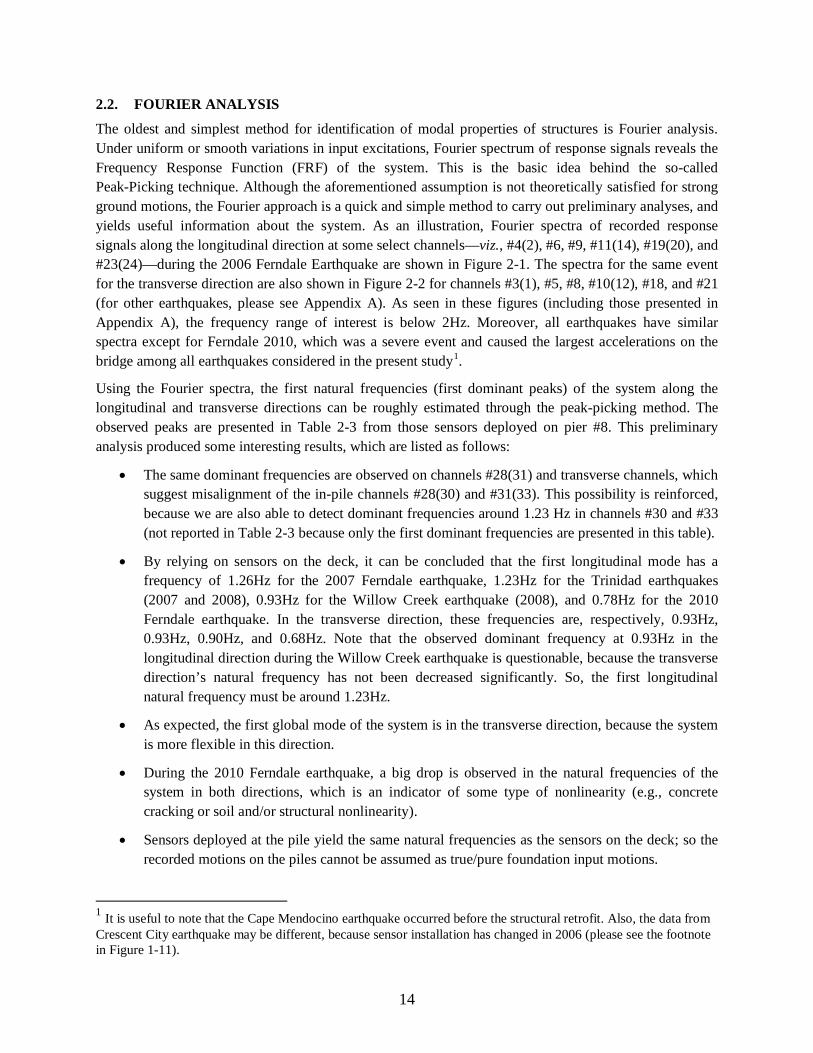
The oldest and simplest method for identification of modal properties of structures is Fourier analysis. Under uniform or smooth variations in input excitations, Fourier spectrum of response signals reveals the Frequency Response Function (FRF) of the system. This is the basic idea behind the so-called Peak-Picking technique. Although the aforementioned assumption is not theoretically satisfied for strong ground motions, the Fourier approach is a quick and simple method to carry out preliminary analyses, and yields useful information about the system. As an illustration, Fourier spectra of recorded response signals along the longitudinal direction at some select channels—viz., #4(2), #6, #9, #11(14), #19(20), and #23(24)—during the 2006 Ferndale Earthquake are shown in Figure 2-1. The spectra for the same event for the transverse direction are also shown in Figure 2-2 for channels #3(1), #5, #8, #10(12), #18, and #21 (for other earthquakes, please see Appendix A). As seen in these figures (including those presented in Appendix A), the frequency range of interest is below 2Hz. Moreover, all earthquakes have similar spectra except for Ferndale 2010, which was a severe event and caused the largest accelerations on the bridge among all earthquakes considered in the present study1.

Using the Fourier spectra, the first natural frequencies (first dominant peaks) of the system along the longitudinal and transverse directions can be roughly estimated through the peak-picking method. The observed peaks are presented in Table 2-3 from those sensors deployed on pier #8. This preliminary analysis produced some interesting results, which are listed as follows:

• The same dominant frequencies are observed on channels #28(31) and transverse channels, which suggest misalignment of the in-pile channels #28(30) and #31(33). This possibility is reinforced, because we are also able to detect dominant frequencies around 1.23 Hz in channels #30 and #33 (not reported in Table 2-3 because only the first dominant frequencies are presented in this table).

• By relying on sensors on the deck, it can be concluded that the first longitudinal mode has a frequency of 1.26Hz for the 2007 Ferndale earthquake, 1.23Hz for the Trinidad earthquakes (2007 and 2008), 0.93Hz for the Willow Creek earthquake (2008), and 0.78Hz for the 2010 Ferndale earthquake. In the transverse direction, these frequencies are, respectively, 0.93Hz, 0.93Hz, 0.90Hz, and 0.68Hz. Note that the observed dominant frequency at 0.93Hz in the longitudinal direction during the Willow Creek earthquake is questionable, because the transverse direction’s natural frequency has not been decreased significantly. So, the first longitudinal natural frequency must be around 1.23Hz.

• As expected, the first global mode of the system is in the transverse direction, because the system is more flexible in this direction.

• During the 2010 Ferndale earthquake, a big drop is observed in the natural frequencies of the system in both directions, which is an indicator of some type of nonlinearity (e.g., concrete cracking or soil and/or structural nonlinearity).

• Sensors deployed at the pile yield the same natural frequencies as the sensors on the deck; so the recorded motions on the piles cannot be assumed as true/pure foundation input motions.

1 It is useful to note that the Cape Mendocino earthquake occurred before the structural retrofit. Also, the data from Crescent City earthquake may be different, because sensor installation has changed in 2006 (please see the footnote in Figure 1-11).

15

The observations above indicate that there are several issues, which must be considered for identification purposes:

• True input motions are not available, so the technique adopted for the identification must consider this limitation.

• System can be considered for identification in two directions separately, but there are some problems about the orientation of the sensors, which must be resolved prior to modal identification.

Table 2-3: Identified first dominant peaks (Hz) from sensors on pier No. 8.

Longitudinal Direction Transverse Direction

Event 31 28 9 11 33 30 8 10

Ferndale 2007 0.93 0.93 1.26 1.26 --- 0.93 0.93 0.93

Trinidad 2007 0.90 0.90 1.23 1.23 --- 0.93 0.93 0.93

Willow Creek 2008 0.90 0.90 0.93 0.93 0.93 0.90 0.90 0.90

Trinidad 2008 --- 0.93 1.23 1.23 --- 0.93 0.93 0.93

Ferndale 2010 0.68 0.68 0.78 0.78 --- --- 0.68 0.68

16

Figure 2-1: Fourier spectra of longitudinal response signals for the Ferndale Offshore earthquake, 2007.

1 2 4 8 20Frequency (Hz)

ch04


ch06


ch09


ch11


ch19


ch23

17

Figure 2-2: Fourier spectra of transverse response signals for the Ferndale Offshore earthquake, 2007.


ch03


ch05


ch08


ch10


ch18


ch21

18

2.3. RECORD CORRECTIONS

As discussed in the previous section and in Chapter 1, the nominal orientations of the in-pile sensors warrant further analysis. To see this in the time-domain, the displacement time histories of the suspicious signals—i.e., channels #31 and #28 in the longitudinal direction, and channels #33 and #30 in the transverse direction—are shown in Figure 2-3 through Figure 2-7 for all of the earthquakes. As these sensors are placed in Pier 8’s piles, signals recorded by the channels on this pier are also shown at the top. Also, the Free-Field Motions (FFMs) in the longitudinal and transverse directions are displayed in these figures. Note that the original horizontal FFMs—i.e., channels #25 and #27—are not aligned with the two principal directions of the bridge, so they are rotated here to produce the two acceleration components along the principal directions.

As seen in Figure 2-3 through Figure 2-7, the time histories of the signals recorded by channels #31 and #28 (longitudinal direction) and channels #33 and #30 (transverse direction) have different appearances from those recorded on the foundation and the bridge deck. Again, this suggests that the orientations of the in-pile sensors are not exactly in the transverse and longitudinal directions of the bridge. It is expedient to note here that CGS had estimated the orientation of channels #31 and #33 and rotated them in the data of Ferndale earthquake 2010 (see, §1.4.1). As seen in Figure 2-7, these channels look fine. Our comparison between the old and the updated data of this earthquake (which is used in this project) shows that CGS has corrected these two channels at this earthquake by simply reversing their directions.

To fix the sensor orientation problems, we will use two different approaches: (i) Fourier analysis, and (ii) correlation analysis. Formulation details of these two methods and their results are presented in the following sub-sections.

(a) Longitudinal direction (b) Transverse direction

Figure 2-3: Recorded responses at pier No. 8 during Ferndale Offshore earthquake, 2007.

19


Figure 2-4: Recorded responses at pier No. 8 during Trinidad earthquake, 2007.


Figure 2-5: Recorded responses at pier No. 8 during Willow Creek earthquake, 2008.


Figure 2-6: Recorded responses at pier No. 8 during Trinidad earthquake, 2008.

20


Figure 2-7: Recorded responses at pier No. 8 during Ferndale earthquake, 2010.

2.3.1 Estimation of sensor orientation using Fourier analysis Due to inertial soil-pile-structure interaction, natural frequencies of a bridge system may be observed in the Fourier spectra of the signals at its support structures, such as abutments and piles. This is certainly the case for the Samoa Bridge, as discussed in Chapter 1 above. Assuming that the dynamic responses of the bridge system along the transverse and longitudinal directions are uncoupled, the piles’ response spectra must exhibit peaks at the same frequencies. Based on this, we can rotate two perpendicular signals—e.g., channels #28 and #30—and compare their Fourier spectra with signals recorded on the deck (for which the sensor orientations are accurately known). Here, we carry out the said rotations in 1-degree increments, and discern the true orientation as the one in which the spectra of the two rotated perpendicular signals have the most distinct peaks that are compatible with values observed in their corresponding deck channels. As an illustration, we present here the Fourier spectra at 0, 15, 30, 45, 60, and 75 degrees for channels #28 and #30 recorded during the Ferndale earthquake, 2007. The same graphs for all other earthquakes are presented in Appendix B.

As seen in Figure 2-8, two signals become more and more distinct from each other in the frequency domain, as the signal are rotated. At a rotation of ~30 degrees (clockwise in top/plan view), the blue curve shows a dominant frequency at 1.26Hz, which is the first natural frequency of the system in the longitudinal direction, and the red curve shows a dominant frequency at 0.93Hz, which is the first natural frequency of the system in the transverse direction. The most important point to note is that at this rotation angle, the red curve does not have a peak at 1.26Hz, and the blue curve one does not have peak at 0.93Hz. As such, it can be concluded that the signals recorded at channels #28 and #30 must be rotated ~30 degrees. The same pattern is observed for other earthquakes (Appendix B), which confirms the results.

21

Figure 2-8: Fourier spectra of rotated components of pile responses recorded in Ferndale Offshore earthquake, 2007.

2.3.2 Estimation of sensor orientation using correlation analysis

The approach presented in the previous section to detect true sensor orientation is essentially qualitative, and here a more accurate and quantitative method based on correlation analysis will be applied to sensor data. This correlation-based approach will seek the particular orientation for which the two rotated perpendicular channels exhibit the least amount of similarity.

0 0.5 1 1.5 2 2.5 3 3.5Frequency (Hz)

Long.Trans.

α = 0o

0 0.5 1 1.5 2 2.5 3 3.5Frequency (Hz)

Long.Trans.

α = 15o

0 0.5 1 1.5 2 2.5 3 3.5Frequency (Hz)

Long.Trans.

α = 30o

0 0.5 1 1.5 2 2.5 3 3.5Frequency (Hz)

Long.Trans.

α = 45o

0 0.5 1 1.5 2 2.5 3 3.5Frequency (Hz)

Long.Trans.

α = 60o

0 0.5 1 1.5 2 2.5 3 3.5Frequency (Hz)

Long.Trans.

α = 75o

22

The cross-correlation technique is nominally used in the time domain for calculating the time-lag between two delayed, but otherwise similar, accelerograms (Bendat and Piersol, 1980). The cross-correlation function measures the similarity between two series (acceleration records here), which are shifted against one another, as a function of delay or time-lag. It displays distinct maxima and minima at particular lag values for which the signals are the most and least correlated, respectively. For detecting the sensor orientations, we will compute the cross-correlation function between to perpendicular signals for every possible orientation; and since they are recorded simultaneously and at the same location, we will use zero time-lag. The true orientation must be the one that yields the least correlated perpendicular signals, and thus the smallest value of the cross-correlation function2.

The cross-correlation function for two 𝑠𝑖(𝑡) and 𝑠𝑗(𝑡) accelerograms at lag 𝜏 = 𝑚∆𝑡 is calculated as

𝑐𝑖𝑗(𝜏) =1𝑁

� 𝑠𝑖(𝑛∆𝑡)𝑁−𝑚

𝑛=1

𝑠𝑗((𝑛 + 𝑚)∆𝑡) (1)

where 𝑚 = 1, 2,⋯ ,𝑁 , ∆𝑡 is the time step, and 𝑁 is number of time samples. It is also possible to calculate 𝑐𝑖𝑗(𝜏) in negative lags, which are indeed obtained by changing 𝑖 and 𝑗 sub-indices at summation above.

Figure 2-9 displays 𝑐𝑖𝑗(0) for each pair of rotated channels #28 and #30 for all earthquakes. As seen, for the default orientation, the signals have a high correlation because their frequency contents are similar and are dominated by the full set of natural frequencies of the system. By rotating the signals, the said similarity decreases and reaches a minimum value around 35 degrees, and then increases again. This pattern is observed for Ferndale 2007, Trinidad 2007, and Willow Creek 2008.

Based on the aforementioned findings, we rotated channels #28 and #30 approximately 35 degrees (clockwise in plan view). Furthermore, we also adopted the corrections made the CGS-Caltrans team for channels #31 and #33 using the 2010 Ferndale earthquake. We apply these corrections to all other earthquake records, and use the rotated data in all subsequent modal identification and model updating studies.

Remarks: For the 2008 Trinidad earthquake, the cross-correlation index did not work well, because of the presence of high-frequency noise in the records. For the 2010 Ferndale earthquake, the index became a minimum at approximately 17 degrees. However, this earthquake should be considered as a special case, because the motion amplitudes were very high; and as will be shown later, there is strong evidence of significant nonlinearity during this event. As such, 2008 Trinidad and 2010 Ferndale data were not used for assessing true sensor orientations.

2 As will be shown later, we can also identify the wave propagation velocity in soil layers in both horizontal and vertical directions through correlation analysis.

23

Figure 2-9: Cross-correlation between two components at different directions.

The corrected (rotated) time histories are shown in Figure 2-10 to Figure 2-14. As seen in these figures, all signals now have similar appearances—that is, a dominant pulse that travels upward is observed.

0 10 20 30 40 50 60 70 80 900

0.1

0.2

Rotation (Deg.)

Cro

ss C

orre

latio

n

Ferndale 2007

0 10 20 30 40 50 60 70 80 900

0.1

0.2

0.3

Rotation (Deg.)

Cro

ss C

orre

latio

n

Trinidad 2007

0 10 20 30 40 50 60 70 80 900

0.1

0.2

Rotation (Deg.)

Cro

ss C

orre

latio

n

Trinidad 2008

0 10 20 30 40 50 60 70 80 900

0.1

0.2

0.3

0.4

Rotation (Deg.)

Cro

ss C

orre

latio

n

Willow Creek 2008

0 10 20 30 40 50 60 70 80 900

0.1

0.2

0.3

0.4

0.5

Rotation (Deg.)

Cro

ss C

orre

latio

n

Ferndale 2010

24


Figure 2-10: Corrected responses recorded during Ferndale Offshore earthquake, 2007.


Figure 2-11: Corrected responses recorded during Trinidad earthquake, 2007.


Figure 2-12: Corrected responses recorded during Willow Creek earthquake, 2008.

25


Figure 2-13: Corrected responses recorded during Trinidad earthquake, 2008.


Figure 2-14: Corrected responses recorded during Ferndale earthquake, 2010.

2.4. SPATIAL VARIATIONS OF THE INPUT MOTIONS

For a large-scale structure like the Samoa Channel Bridge, the issue of multiple support excitations is an important concern. Previously, it was shown that the recorded signals on the pile-tip contain the natural frequencies of the system, and thus, they cannot be considered as pure input motions. Even by neglecting such inertial soil-structure interaction effects, these signals cannot be assumed as input motions for the entire bridge, if they exhibit a spatial variation along the bridge’s support structures.

Spatial variation is dominated by two factors: (i) spatial variation of the site’s soil properties, and (ii) wave passage effects. If seismic waves that are affecting the structure are primarily vertically propagating (from a bedrock) and horizontally polarized shear waves, then spatial variations can be omitted. We seek to quantify the spatial variations of the seismic excitations for the Samoa Bridge, to the extent possible with its currently available data.

Figure 2-15 displays the Fourier spectra of the signals recorded at both ends of the bridge in the longitudinal direction. The figures for the transverse direction are not shown, as there is no sensor in this direction outside of the bridge on the Samoa side. Also, no graph is shown for the Ferndale earthquake of

26

2010, because we do not have data from channel #24 during this earthquake. As this figure indicates, the recorded signals at both sides have different frequency content; that is, the bridge has probably experienced different excitations at different piers. Unfortunately, the available data are not quite sufficient to confirm this hypothesis.

The time domain versions of the same signals can be used to investigate if there is any delay between the excitations experienced at the two ends of the bridge. For this purpose, we calculate such delay between two signals recorded at both abutments—viz., channels #2 and #24 for the longitudinal direction, and #1 and #22 for the transverse direction (for the transverse direction, the results may be unreliable, because channel #22 is placed on the deck). To increase the reliability of these results, delays between two signals (for each direction) are calculated using two methods. In the first method, as shown as an example for the longitudinal direction in Figure 2-16, the time delay is detected from the recorded displacement time-histories. In the second approach, the cross-correlation technique is employed, as shown in Figure 2-17. Results of both methods are presented in Table 2-4. As these abutment recordings are nominally supposed to be independent from the bridge’s dynamic properties, we also included data from two old earthquakes, i.e., Cape Mendocino earthquake 2000, and Crescent City earthquake 2005. As seen, time delays obtained using both methods are in close agreement, except a for few cases.

Table 2-4: Wave propagation study.

Event Date Transverse Delay (ms) Longitudinal Delay (ms) Propagation

Angle (Deg.) Direct Correlation Direct Correlation

Cape Mendocino 03/16/00 80 60 80 −10 52 Crescent City Offshore 06/14/05 170 160 70 140 13

Ferndale Offshore 02/26/07 90 130 80 90 44 Trinidad 06/24/07 190 210 170 185 4

Willow Creek 04/29/08 −170 −65 −160 −75 31 Trinidad 08/16/08 150 205 150 150 56

Ferndale Area 01/09/10 --- --- --- 46

To see the relation between time delays and the locations of the earthquakes’ source, Figure 2-18 is presented. As this figure shows, if we draw a line between the earthquake sources and the center of the bridge, the wave arrival/incidence angles with respect to the bridge orientation can be found. Of course, this is a highly simplified approximation wherein the earthquakes’ sources are assumed to be point sources. The calculated propagation angles are shown in the last column of Table 2-4 as well. As seen, this angle is a minimum for the Trinidad earthquake (2007), and in agreement with this result, the time delay is also a maximum.

27

(a) Ferndale earthquake, 2007

(b) Trinidad earthquake, 2008

(c) Willow Creek earthquake, 2008

(d) Trinidad earthquake, 2008

Figure 2-15: Fourier spectra of recorded signals at both ends of the bridge.


ch02


ch24


ch02


ch24


ch02


ch24


ch02


ch24

28

(a) Cape Mendocino, 2000 (b) Crescent City, 2005

(c) Ferndale, 2007 (d) Trinidad, 2007

(e) Willow Creek, 2008 (f) Trinidad, 2008

Figure 2-16: Time-delay observed between two sides of the bridge.

29

Figure 2-17: Cross-correlation between two signals recorded at both sides of the bridge.

Figure 2-18: Arrival directions.

Cap

e.20

00

Longitudinal Transverse

Fern

.20

07Tr

in.

2007

Trin

.20

08

-2 -1 0 1 2Lag (sec.)

Will.

2008

-2 -1 0 1 2Lag (sec.)

Cre

s.20

05

-126 -125.6 -125.2 -124.8 -124.4 -124 -123.6 -123.2 -12340.2

40.4

40.6

40.8

41

41.2

41.4

41.6

Longitude

Latit

ude

Cerescent City2005

Trinidad2008

Trinidad2007

Samoa Bridge

Willow Creek2008

Ferndale2007

Cape Mendocino2000

Ferndale Offshore2007

Eureka2002

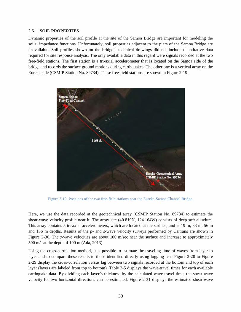
30

2.5. SOIL PROPERTIES

Dynamic properties of the soil profile at the site of the Samoa Bridge are important for modeling the soils’ impedance functions. Unfortunately, soil properties adjacent to the piers of the Samoa Bridge are unavailable. Soil profiles shown on the bridge’s technical drawings did not include quantitative data required for site response analysis. The only available data in this regard were signals recorded at the two free-field stations. The first station is a tri-axial accelerometer that is located on the Samoa side of the bridge and records the surface ground motions during earthquakes. The other one is a vertical array on the Eureka side (CSMIP Station No. 89734). These free-field stations are shown in Figure 2-19.

Figure 2-19: Positions of the two free-field stations near the Eureka-Samoa Channel Bridge.

Here, we use the data recorded at the geotechnical array (CSMIP Station No. 89734) to estimate the shear-wave velocity profile near it. The array site (40.819N, 124.164W) consists of deep soft alluvium. This array contains 5 tri-axial accelerometers, which are located at the surface, and at 19 m, 33 m, 56 m and 136 m depths. Results of the p- and s-wave velocity surveys performed by Caltrans are shown in Figure 2-30. The s-wave velocities are about 100 m/sec near the surface and increase to approximately 500 m/s at the depth of 100 m (Ada, 2013).

Using the cross-correlation method, it is possible to estimate the traveling time of waves from layer to layer and to compare these results to those identified directly using logging test. Figure 2-20 to Figure 2-29 display the cross-correlation versus lag between two signals recorded at the bottom and top of each layer (layers are labeled from top to bottom). Table 2-5 displays the wave-travel times for each available earthquake data. By dividing each layer’s thickness by the calculated wave travel time, the shear wave velocity for two horizontal directions can be estimated. Figure 2-31 displays the estimated shear-wave

31

velocity values for a weak earthquake (Cape Mendocino 03/16/2000) and a strong earthquake (Ferndale 01/09/2010), as well as values estimated by Caltrans, which are all in reasonable agreement. It should be noted that the similar analyses have been carried out and reported recently by Ada (2013).

Figure 2-20: Cross-correlations of recorded signals at soil layers for Cape Mendocino earthquake, 2000.

Figure 2-21: Cross-correlations of recorded signals at soil layers for Eureka Offshore earthquake, 2000.

32

Figure 2-22: Cross-correlations of recorded signals at soil layers for Ferndale Offshore earthquake, 2000.

Figure 2-23: Cross-correlations of recorded signals at soil layers for Crescent City earthquake, 2005.

33

Figure 2-24: Cross-correlations of recorded signals at soil layers for Ferndale Offshore earthquake, 2007.

Figure 2-25: Cross-correlations of recorded signals at soil layers for the Trinidad earthquake, 2007.

34

Figure 2-26: Cross-correlations of recorded signals at soil layers for Ferndale earthquake, 1/9/2010.

Figure 2-27: Cross-correlations of recorded signals at soil layers for Ferndale earthquake, 2/4/2010.

35

Figure 2-28: Cross-correlations of recorded signals at soil layers for Weitchpec earthquake, 2012.

Figure 2-29: Cross-correlations of recorded signals at soil layers for Blue Lake earthquake, 2012.

36

Figure 2-30: Suspension logging test results from the Geotechnical Array CSMIP Station 89734.

Figure 2-31: Shear wave velocities identified using Earthquake data and the Caltrans estimated values.

Table 2-5: Wave travel times (sec) obtained through the wave propagation study.

Layer 1 Layer 2 Layer 3 Layer 4

L T V L T V L T V L T V

Cape Mendocino 3/16/2000 0.000 0.010 0.000 0.040 0.040 0.000 0.050 0.050 0.010 0.170 0.170 0.030

Eureka Offshore 9/22/2000 0.100 0.100 0.010 0.050 0.050 0.000 0.060 0.060 0.010 0.170 0.160 0.110

Ferndale Offshore 12/27/2000 0.090 0.100 0.150 0.260 0.330 0.000 0.380 0.380 0.020 0.170 0.160 0.550

Crescent City 6/14/2005 0.090 0.070 0.000 0.030 0.040 0.000 0.040 0.040 0.000 0.170 0.160 NR

Ferndale 2/26/2007 0.090 0.090 0.000 0.040 0.040 0.000 0.060 0.060 0.010 0.170 0.160 NA

Trinidad 6/24/2007 NR* NR 0.000 0.030 0.020 0.000 0.045 0.010 0.005 0.170 0.175 NA

Ferndale 1/9/2010 0.110 0.140 0.000 0.050 0.060 0.000 0.060 0.060 0.000 0.180 0.180 NA

Ferndale 2/4/2010 0.090 0.000 0.010 0.040 0.050 0.000 0.050 0.050 0.000 0.170 0.170 NA

Weitchpec 2/13/2012 0.100 0.105 0.005 0.050 0.045 0.000 0.055 0.055 0.005 0.170 0.165 NA

Blue Lake 10/21/2012 0.105 0.105 NR 0.265 0.260 0.005 0.065 0.060 0.015 0.170 0.175 NA

• Not Reliable, ** Not Available

37

2.6. INITIAL FINITE ELEMENT MODELING

An initial, albeit detailed, three-dimensional finite element model of the Samoa Bridge, including its pile foundations, was created using all available structural details (Figure 2-32) using CSIBridge (CSI, 2014). The soil’s flexibility was represented using soil macroelements whose depth-varying properties (Matlock, 1970; API, 1993) were assigned using site-specific geotechnical data (CSMIP, 2012) and the bridge plan titled “Log of Test Borings.” The soil springs have nonlinear backbone curves, and display hysteretic response upon unloading. Figure 2-33 displays the final FE model complete with its nonlinear soil springs.

Figure 2-32: Detailed three-dimensional model of the Samoa Bridge using CSIBridge.

The bridge deck and the pile-caps were modeled with shell elements; and the columns were modeled with beam elements. The piles were also modeled with beam elements, and the nonlinear soil springs attached at discrete locations represent the lateral and vertical interaction between the piles and their surrounding soil media. The boundary conditions at the abutments were modeled using a “friction isolator” to simulate the elastomeric pads, and to decouple the superstructure and the abutment backwall from the pile cap. The isolator was fixed in the vertical direction only. The longitudinal abutment-backfill reaction was modeled by a series of nonlinear link-elements that were distributed along each abutment backwall using the experimentally validated formulation provided by Shamsabadi et al. (2010). The abutment springs were offset by 2.54 cm (1 in.) to take the abutment expansion gap into account.

38

Figure 2-33: Detailed three-dimensional model of the Samoa Bridge featuring nonlinear soil springs.

Remark: In a parallel effort, a second FE model was also developed with the Midas Civil software (MIDASoft, 2012) to explore the relative accuracy and computational efficient of direct and substructure methods. Figure 2-34 displays these two extra models, whose further details can be found in (Shamsabadi and Taciroglu, 2013). The modal properties and nonlinear time history responses of these two Midas models were found to agree well with those obtained using the CSIBridge model, which indicated that all of the developed (i.e., CSIBridge vs. Midas, and direct vs. substructure) FE models represent essentially the same soil-structure system. Details of the said comparisons are omitted here for brevity.

(a) direct model

(b) substructure model

Figure 2-34: Direct and substructure finite element models of the Samoa Bridge created using MIDAS.

39

Chapter 3 MODAL IDENTIFICATION

3.1. INTRODUCTION

Direct analyses are provisioned in most existing seismic design guideline documents on bridges—that is, based on geometric and material properties of the superstructure and soil, a model is constructed for linear/nonlinear quasi-static/dynamic analyses (see, for example, Aviram et al., 2008; Kaviani et al., 2014). Ideally, all analytical/numerical models are valid in that their predictions are accurate realizations of the actual behavior of the bridges they represent, and that these predictions will match direct physical measurements from strong shaking events, if such measurements are available.

For bridge structures, the earliest recordings were made in 1979 when two instrumented bridges in California were shaken by different earthquakes. Wilson (1984) presented one of the first studies on recorded vibration data and studied the earthquake response of a multi-span bridge. He employed an identification technique proposed by Beck (1979), and was able to extract a number of natural frequencies, damping ratios and modal contribution factors (but not mode shapes). Wilson used free-field motions recorded at the ground surface as input excitations and extracted the aforementioned modal properties for the few first modes. This and other similar initial studies—and several major earthquakes—prompted a statewide program, and in 1994, Caltrans began to instrument bridges across California (Hipley and Huang, 1997). Today there are at least 59 bridges in California with permanent seismic instruments, and strong motion data from these stations are publicly available. Data from California’s instrumented bridges have been used in a number of studies on model validation (Goel, 1997; Arici and Mosalam, 2003) and structural health monitoring (Seim and Giacomini, 2000; Smyth et al., 2000, 2003; Masri et al., 2004; Anderson et al., 2007).

In earlier studies on California’s instrumented bridges, soil-structure interaction (SSI) hasn’t been explored with requisite detail and appropriate methods. The particular challenge in this area has been the lack of proper output-only methods, because recorded translational foundation responses are not true input motions (Stewart and Fenves, 1998) and thus input-output methods are not applicable, and existing output-only methods are based on the unknown input being stationary, which is not true for strong motion events. Free-Field Motions (FFMs) recorded nearby the structure cannot be used for modal identification of soil-structure systems either, due to kinematic interaction effects. This phenomenon was already observed for the Samoa Bridge as discussed in Chapter 2. Here to show the presence of SSI effects, the Fourier spectra of free-field motions and responses recorded on the bridge are compared in Figure 3-1. To have consistent signals, the horizontal free-field channels are rotated to be oriented in the transverse and longitudinal directions of the bridge, and the longitudinal component is shown in Figure 3-1. As this figure clearly shows, both the on-bridge and free-field signals have the same dominant frequency3 and as will be shown later in this chapter, this dominant frequency is related to the first longitudinal frequency of the bridge-foundation-soil system during this earthquake. That is, the vibration of the system affects what had been assumed to be the “free-field” motion. It is important to note here that basin effects cannot produce this dominant frequency, because it is observable even when the system is undergoing free vibrations. Moreover, this dominant frequency is not observed in the transverse direction, because the bridge does not vibrate monolithically in this direction.

3 During the Ferndale earthquake, the system behaves nonlinearly, so this frequency is actually an average value.

40

The matter is further complicated by the fact that the Samoa Bridge likely experiences multiple input motions, and thus the traditional input-output identification methods are no longer applicable. Given these observations, a new output-only identification technique developed by the PI and his co-workers is employed. This method is an extension of a method, which had been already proposed by the PIs group for ambient data (Abazarsa et al. 2013ab; Ghahari et al. 2013a). So, first, details of the method for ambient data are described. Although there are several output-only identification methods in the literature—e.g., Eigensystem Realization Algorithm (ERA) (Juang and Pappa 1985), Stochastic Subspace Identification (SSI) method (Van Overschee and De Moor 1993), and Frequency Domain Decomposition (FDD) method (Brincker et al. 2001), the proposed method is used in this project for modal identification from ambient data to maintain consistency between identification results from both ambient and earthquake data. Subsequently, details of the technique for output-only identification from earthquake data are presented.

Figure 3-1: Fourier spectra of the free-field motion (rotated to the bridge-longitudinal direction) and the bridge

response (longitudinal direction) recorded during the 2010 Ferndale earthquake.

3.2. MODAL IDENTIFICATION TECHNIQUE FOR AMBIENT DATA

Under free vibration conditions, the structural response may be written in modal space, as in

𝒙(𝑡) = 𝞍 𝒒(𝑡) (2)

where 𝒙(𝑡) is the vector of response signals; 𝞍 is the real-valued mode shape matrix; and 𝒒(𝑡) is the vector of modal coordinates. The modal coordinate is the response of a single degree-of-freedom (DOF) system that bears the same natural frequency, 𝑓𝑛𝑖, and damping ratio, 𝜉𝑖, with the ith mode of the structure. That is,

𝑞𝑖(𝑡) = 𝛼𝑖𝑒−𝜉𝑖𝜔𝑛𝑖𝑡sin (𝜔𝑑𝑖𝑡 + 𝜃𝑖) (3)

41

where 𝜔𝑛𝑖 = 2𝜋𝑓𝑛𝑖, 𝜔𝑑𝑖 = 𝜔𝑛𝑖�1 − 𝜉𝑖2, 𝜃𝑖 and 𝛼𝑖 are two constants that represent the initial conditions

and contribution of the ith mode. As described in Appendix C, it can be shown that under ambient excitations, the cross-correlations of acceleration responses relative to a reference response have a form that is similar to modal expansion (James et al. 1993 and 1995). To wit,

𝑅𝑖𝑗(𝜏) = �𝜑𝑖𝑟𝐶𝑗𝑟𝑚𝑟𝜔𝑑𝑟

𝑒−𝜉𝑟𝜔𝑛𝑟𝜏 sin�𝜔𝑑𝑟𝜏 + 𝜃𝑗𝑟� for 𝑖, 𝑗 = 1, … ,𝑛𝑚

𝑟=1

(4)

where 𝑅𝑖𝑗(𝜏) is the correlation function of the response at point i relative to the reference point j; 𝜏 is the time-lag; 𝑚𝑟 is the rth modal mass; 𝜑𝑖𝑟 is the modal deformation of point i in the rth mode; and 𝐶𝑗𝑟 and 𝜃𝑗𝑟 are time-independent parameters. Also, 𝑛 and 𝑚 denote the number of instrumented degrees of freedom, and the number of modes, respectively. Clearly, the decaying sinusoid terms in Eq. (4) are similar to those in Eq. (3). Thus, the correlation responses can be treated as free vibration responses.

In both the cases of response signals or correlation signals, the 𝑒−𝜉𝑖𝜔𝑛𝑖𝑡sin (𝜔𝑑𝑖𝑡) terms are approximately uncorrelated to each other because ∫ sin(𝜔𝑖𝑡) sin�𝜔𝑗𝑡� 𝑑𝑡

+∞−∞ = 0. The aforementioned

fact imply that the covariance matrix of the response signals at non-zero time lags, i.e., 𝐑𝒙(𝜏), is

𝐑𝒙(𝜏) = 𝞍𝐑𝒒(𝜏)𝞍𝑇 (5)

where 𝐑𝒒 is covariance matrix of modal coordinates, which is a diagonal matrix whose diagonal entries are auto-correlation of modal coordinates, and superscript T denotes the transpose of a vector. The right-hand side of this expression is an EigenValue Decomposition (EVD). However, a suitable value of 𝜏 for which 𝐑𝒙(𝜏) is a positive definite or positive semi-definite matrix is not known a priori. As such, it is expedient to diagonalize a set of 𝐑𝒙(𝜏) simultaneously for several time lags. Such a Joint Approximate Diagonalization (JAD) can be accomplished with the Jacobi method (Cardoso and Souloumiac1996). After identification of mode shape matrix, natural frequencies and damping ratios can be easily estimated from modal coordinate signals using any SDOF identification method (e.g., Yang et al. 2003), which are recovered through

𝒒(𝑡) = 𝞍#𝒙(𝑡) (6)

where the superscript # denotes the Moore–Penrose pseudo-inverse. The aforementioned method, which is named Second Order Blind Identification (SOBI), was originally proposed by Belouchrani et al. (1997) as a technique for solving Blind Source Separation (BSS) problems in electrical engineering for estimating individual source signals from their recorded mixtures. Recently, this method has found use in ambient modal identification of mechanical systems and civil structures (Antoni 2005; Kerschen et al. 2007; Poncelet et al. 2007; Zhou and Chelidze 2007; McNeill and Zimmerman 2008). This particular extraction method works without having the sources, here modal coordinates, or the mixing process, here mode shape matrix—hence the term, blind—and employs second-order statistics of recorded response signals to recover the modal coordinate signals and the mode shape matrix. Nevertheless, conventional versions of SOBI methods are limited to determined or overdetermined problems, in which the number of active modes is equal to or less than the number of recorded signals. For civil structures (e.g., tall

42

buildings, long-span bridges, etc.), this constraint is often prohibitive. Recently, P.I. and his co-workers (Abazarsa et al. 2013ab) have employed a simultaneous matrix diagonalization procedure that is proposed by De Lathauwer and Castaing (2008) through which Eq. (5) can be treated as a Parallel Factor (PARAFAC) (Harshman 1970) decomposition. PARAFAC is a multilinear algebra technique for decomposing a tensor into a sum of rank-one tensors (Nion et al. 2010). In what follows, a summary of this approach is presented.

First, let us define a third-order tensor as �𝐑�𝒙�𝑖𝑗𝑘 ≔ [𝐑𝒙(𝜏𝑘)]𝑖𝑗 where i, j = 1, …, n, and k = 1, …, K.

Here, 𝐾 is the number of selected time lags; and [•]𝑖𝑗 denotes the entry placed in ith row and jth column of the matrix in the square bracket. Also, let us define a new matrix �𝐑𝒒�𝑘𝑟 ≔ �𝐑𝒒(𝜏𝑘)�

𝑟𝑟 where r = 1, …,

m, and k = 1, …, K (here the repeated index r marks the position of a diagonal element). Based on Eq. (5), each entry of tensor �𝐑�𝒙�𝑖𝑗𝑘 can be written as,

�𝐑�𝒙�𝑖𝑗𝑘 = �[𝞍]𝑖𝑟[𝞍]𝑗𝑟�𝐑𝒒�𝑘𝑟

𝑚

𝑟=1

(7)

This equation shows that by decomposing the third-order tensor 𝐑�𝒙 into 𝑚 rank-one tensors, the mixing matrix can be identified. The rank of a tensor is defined as the minimal number of rank-one tensors into which a higher order tensor can be decomposed; thus, the rank of 𝐑�𝒙 is 𝑚. In contrast to the matrix case, PARAFAC can result in a unique decomposition even when the rank-one terms are not mutually orthogonal or even when the rank is greater than the smallest tensor dimension; that is, the underdetermined problems can now be solved.

The tensor 𝐑�𝒙 can be denoted through a matrix representation as follows,

�𝐑𝒙�(𝑖−1)𝑛+𝑗,𝑘∶= �𝐑�𝒙�𝑖𝑗𝑘 (8)

Based on Eq. (7), this new 𝑛2 × 𝐾 matrix 𝐑𝒙 can be represented as a Khatri-Rao product (Khatri and Rao 1968), as in

𝐑𝒙 = (𝞍⨀𝞍)𝐑𝒒𝑇 (9)

where ⨀ denotes the Khatri-Rao product operator. As both 𝞍⨀𝞍 and 𝐑𝒒 are full column rank matrices, the number of modes 𝑚 is simply equal to the rank of 𝐑𝒙, which can be easily determined through a Singular Value Decomposition (SVD). That is, the number of significant singular values indicates the number of contributing modes. Considering only the first 𝑚 significant singular values, the SVD of 𝐑𝒙 can be stated as,

𝐑𝒙 = 𝐔 𝚫 𝐕𝑇 (10)

where 𝐔 and 𝐕 are 𝑛2 × 𝑚 and 𝐾 × 𝑚 column-wise orthonormal matrices, respectively; and 𝚫 is an 𝑚 × 𝑚 positive-definite diagonal matrix. By combining Eqs. (9) and (10), we may conclude that there exist an 𝑚 × 𝑚 non-singular unknown matrix 𝐅 such that

43

𝞍⨀𝞍 = 𝐔 𝚫 𝐅 (11)

𝐑𝒒 = 𝐕 𝐅−𝑇 (12)

It is clear that if 𝐅 can be determined, then the mode shape matrix 𝞍, and the autocorrelation of unknown modal coordinates 𝐑𝒒 can be easily estimated. The following procedure is used to compute this matrix.

Let us first define 𝐇 ∶= 𝐔 𝚫, which is an 𝑛2 × 𝑚 matrix. Then let us define 𝐇𝑟 , which is an 𝑛 × 𝑛 matrix, defined through the index mapping [𝐇𝑟]𝑖𝑗 ∶= [𝑯𝑟](𝑖−1)𝑛+𝑗 where r = 1, …, m and 𝑯𝑟 is the rth column of matrix 𝐇. It follows from Eq. (11) that the matrix 𝐇𝑟 can be written as a linear combination of rank-one matrices, as in

𝐇𝑟 = �𝟇𝑘𝟇𝑘𝑇

𝑚

𝑘=1

[𝐅−1]𝑘𝑟 𝑟 = 1, …, 𝑚 (13)

where 𝟇𝑘 is the kth column of matrix 𝞍. From the set of 𝑚 matrices {𝐇𝑟}, a set of 𝑚2 tensors ��𝐏�𝑠𝑡�∶= 𝜑(𝐇𝑠,𝐇𝑡)� where s, t = 1, …, m, can be defined, where 𝜑 is a symmetric and bilinear mapping through which it is possible to determine whether a matrix is rank-one or not. Each �𝐏�𝑠𝑡� tensor is defined as follows,

�𝐏�𝑠𝑡�𝑖𝑗𝑘𝑙 ∶= [𝐇𝑠]𝑖𝑗[𝐇𝑡]𝑘𝑙 + [𝐇𝑡]𝑖𝑗[𝐇𝑠]𝑘𝑙 − [𝐇𝑠]𝑖𝑙[𝐇𝑡]𝑘𝑗 − [𝐇𝑡]𝑖𝑗[𝐇𝑠]𝑘𝑙 𝑖, 𝑗, 𝑘, 𝑙 = 1, … , 𝑛, (14)

where 𝜑(𝐇𝑠,𝐇𝑠) = 𝟎� if and only if the rank of 𝐇𝑠 is at most one.

We can then define a set of 𝑚 × 𝑚 symmetric matrices 𝐌𝑟 ∶= 𝐅 𝚲𝑟 𝐅𝑇 where 𝚲𝑟 are arbitrary diagonal matrices, and r = 1, …, m . It can be shown that ∑ [𝐌𝑟]𝑠𝑡�𝐏�𝑠𝑡�𝑚

𝑠,𝑡=1 = 𝟎� where r = 1, …, m (De Lathauwer 2006), and by using this set of linear homogenous equations, the 𝐌𝑟 matrices can be determined.

It follows then that the matrix 𝐅 can be easily identified through any existing non-unitary JAD technique—such as that described in (Souloumiac 1999)—because the matrix 𝐅 simultaneously diagonalizes each of these 𝐌𝑟 matrices. Now, by defining C ∶= 𝐇 𝐅, the column 𝟇𝑘 can be estimated, up to a scaling factor, as the left singular-vector associated with the largest singular value of 𝐁𝑘 where [𝐁𝑘]𝑖𝑗 ∶= [𝑪𝑘](𝑖−1)𝑛+𝑗, and 𝑪𝑘 denotes the kth column of matrix 𝐂.

By employing aforementioned algorithm, the mode shape matrix is identified. However, the extracted results are unique only if the following inequality is satisfied (Stegeman et al. 2006),

𝑚(𝑚− 1)2

≤𝑛(𝑛 − 1)

4�𝑛(𝑛 − 1)

2+ 1� −

𝑛!(𝑛 − 4)! 4!

1{𝑛≥4} (15)

where

1{𝑛≥4} ∶= �0, if 𝑛 < 4,1, if 𝑛 ≥ 4. (16)

44

The number of identifiable modes (m) for a given number of sensors (n)—calculated using Eq. (15)—are rounded down to the nearest integer, and are shown in Table 3-1, for up to 12 sensors.

Table 3-1: Number of identifiable modes with a limited number of sensors.

Number of sensors (n) 2 3 4 5 6 7 8 9 10 11 12

Number of identifiable modes (m) 2 4 6 10 15 20 26 33 41 49 59

The identifiability criterion given above is a general condition for random component matrices; and this may not yield to satisfactory identification results for civil structures, unless the sensors are distributed along the structure properly.

Contrary to the determined or the overdetermined cases, modal coordinates cannot be recovered using simple matrix inversion after obtaining the mode shape matrix, because mode shapes are no longer invertible due to incomplete instrumentation. This problem may be circumvented by using the diagonal matrices Rq(τk) that are recovered through the PARAFAC decomposition. Indeed, these matrices contain autocorrelations of the original modal coordinates, so the obtained lag-history signals can represent the time-histories of modal coordinates, because the autocorrelation of a signal—such as those shown in Eqs. (3) and (4)—is self-similar; i.e., its autocorrelation has the same frequency and damping ratio as the original signal. However, the artifacts due to windowing, which is an essential part of the method, smears the damping ratio identification from the recovered modal coordinates’ auto-correlation. To extract the damping ratios, the post-processing technique proposed in (Abazarsa et al., 2013b) can be employed.

3.3. MODAL IDENTIFICATION TECHNIQUE FOR EARTHQUAKE DATA

The governing equations of motion for an N Degree-Of-Freedom (DOF) system with 𝑛 instrumented DOFs, which is excited by a 𝑞 ground acceleration, �̈�𝑔(𝑡) = ��̈�𝑔,1(𝑡),⋯ , �̈�𝑔,𝑞(𝑡)�

𝑇, can be expressed as

follows,

𝐌�̈�(𝑡) + 𝐂�̇�(𝑡) + 𝐊𝒙(𝑡) = −𝐌𝐋�̈�𝑔(𝑡) (17)

where 𝐌, 𝐂, and 𝐊 are the constant N×N mass, proportional damping and stiffness matrices of the system, respectively. The vector 𝒙(𝑡) contains the relative displacement responses of the system at all DOFs; and 𝐋 is the influence matrix (Chopra, 1995). The absolute acceleration of structure at 𝑛 instrumented DOFs is

�̈�𝑡(𝑡) = �̈�(𝑡) + 𝒍�̈�𝑔(𝑡), (18)

and can be expressed in modal space as

�̈�𝑡(𝑡) = 𝞍�̈�(𝑡) (19)

where 𝛟 is an 𝑛 × 𝑚 real-valued mode shape matrix whose i-th column (𝝓𝑖) is the i-th mode shape; and �̈�(𝑡) is a vector that contains the absolute acceleration modal coordinates whose i-th row is the absolute

45

acceleration response of a SDOF system with the natural frequency, 𝜔𝑛 , and damping ratios, 𝜉 , corresponding to the i-th mode. Also 𝑚 ≤ 𝑁 is the number of contributing modes.

These modal coordinates are non-stationary signals, as they are produced under non-stationary input motions. At time 𝑡 and lag 𝜏 , the correlation matrix of the recorded signals, �̈�𝑡(𝑡), is related to the correlation matrix of �̈�(𝑡) can be written as

𝐑�̈�𝑡�̈�𝑡(𝑡, 𝜏) = 𝞍 𝐑�̈��̈�(𝑡, 𝜏) 𝞍𝑇. (20)

where superscript T indicates a matrix/vector transpose. Calculating the Fourier Transform of both sides of Eq. (19), we get

𝐃�̈�𝑡�̈�𝑡(𝑡, 𝑓) = 𝞍 𝐃�̈��̈�(𝑡,𝑓) 𝞍𝑇 (21)

where 𝐃�̈�𝑡�̈�𝑡(𝑡,𝑓)and 𝐃�̈��̈�(𝑡, 𝑓) are, respectively, Spatial Wigner-Ville Distribution (SWVD) matrices of response and modal coordinate signals.

As described by Ghahari et al. (2013c), the time-frequency points can be categorized into three types:

• Single Auto-term TF Point (SATFP): At these points, only one mode is present. Thus, SWVD matrices of modal coordinates, 𝐃�̈��̈�(𝑡,𝑓), are diagonal with only one non-zero diagonal element, which represents the energy of the active mode.

• Multiple Auto-term TF Point (MATFP): At these points, several modes are present. Thus, auto-WVDs of several modes are non-zero, as well as their cross-WVDs4. Therefore, SWVS matrices of the modal coordinates, 𝐒�̈��̈�(𝑡, 𝑓), have non-zero diagonal and off-diagonal elements.

• Cross-Term TF Point (CTTFP): At these points, the cross-WVSs of modal coordinates are non-zero, while their corresponding auto-WVSs are zero. Therefore, at such points, 𝐒�̈��̈�(𝑡, 𝑓) matrices are off-diagonal.

At SATFPs (and some of the MATFPs) wherein the cross-WVDs are zero, 𝐃�̈��̈�(𝑡, 𝑓) matrices are diagonal. Therefore, per Eq. (21), the mode shape matrix and the SWVDs of the modal coordinates can be estimated through a diagonalization process of 𝐃�̈�𝑡�̈�𝑡(𝑡, 𝑓) as proposed by P.I. and his co-workers (Ghahari et al. 2013b) where a Joint Approximate Diagonalization (JAD) procedure (Cardoso and Souloumiac, 1996) was used for simultaneously diagonalizing the 𝐃�̈�𝑡�̈�𝑡(𝑡,𝑓) matrices at all SATFPs. However, the aforementioned JAD is only applicable for determined or over-determined cases, wherein the number of active modes is less than or equal to the number of response signals. To extend this method for underdetermined problems, same procedure described above for ambient data can be used with a few modifications. That is, replacing correlation matrices by time-frequency matrices in the PARAFAC method and following exactly the same process. Hence, only general relations are presented here.

In the first step, the SWVD matrices at the chosen SATFPs/MATFPs are used to construct a third-order tensor as in �𝐃��̈�𝑡�𝑖𝑗𝑘 ≔ [𝐃�̈�𝑡�̈�𝑡(𝑡𝑘,𝑓𝑘)]𝑖𝑗 where i, j = 1, …, n, and k = 1, …, K, where K is the total

4 It is theoretically possible to find time-frequency points wherein the auto-TFDs of several signals are non-zeros, while their cross-TFDs are zero (Belouchrani, 2013).

46

number of selected time-frequency points. Then, a new matrix is defined as �𝐃�̈��𝑘𝑟 ≔ �𝐃�̈��̈�(𝑡𝑘, 𝑓𝑘)�𝑟𝑟

where r = 1, …, m, and k = 1, …, K. Per Eq. (21), each element of �𝐃��̈�𝑡�𝑖𝑗𝑘 can be expressed as,

[𝐃��̈�𝑡]𝑖𝑗𝑘 = �[𝞍]𝑖𝑟[𝞍]𝑗𝑟

𝑚

𝑟=1

�𝐃�̈��𝑘𝑟. (22)

Eq. (22) implies that 𝐃��̈�𝑡 can be decomposed into 𝑚 rank-one tensors, and that the mode shape matrix can be identified in this manner. To wit, the tensor 𝐃��̈�𝑡 can be expressed as a generalized SWVD matrix as in,

�𝐃�̈�𝑡�(𝑖−1)𝑛+𝑗,𝑘∶= �𝐃��̈�𝑡�𝑖𝑗𝑘. (23)

The Khatri-Rao representation of this 𝑛2 × 𝐾 matrix (𝐃�̈�𝑡), is given as

𝐃�̈�𝑡 = (𝞍⨀ 𝞍)𝐃�̈�𝑇 (24)

The singular value decomposition of 𝐃�̈�𝑡 is simply,

𝐃�̈�𝑡 ≈ 𝐔 𝚫 𝐕𝑇 (25)

where 𝐔 and 𝐕 are 𝑛2 × 𝑚 and 𝐾 × 𝑚 column-wise orthonormal matrices, respectively; 𝚫 is an 𝑚 × 𝑚 positive-definite diagonal matrix; and m is the number of significant eigenvalues chosen. Eqs. (24) and (25) together imply that there exist an 𝑚 × 𝑚 non-singular unknown matrix 𝐅 such that

𝞍 ⨀𝞍 = 𝐔 𝚫 𝐅 (26)

𝐃�̈� = 𝐕 𝐅−𝑇 (27)

By computing the matrix 𝐅, the mode shape matrix 𝞍 and the auto-WVD matrix of the unknown modal coordinates at selected SATFPs, 𝐃�̈�, can be easily estimated. However, it is more desirable to extract the auto-WVD of modal coordinates at all time-frequency points. Therefore, after identifying the mode shapes, we herein employ the subspace approach suggested by Ghahari et al. (2013c) to recover modal coordinates’ auto-WVD.

In practice, the discrete form of the SWVD matrices of response signals can be calculated as (Boashash, 2003)

𝐃�̈�𝑡�̈�𝑡(𝑡, 𝑓) = � � �̈�𝑡(𝑡 + 𝑚 + 𝑙) �̈�𝑡𝐻(𝑡 + 𝑚− 𝑙) 𝑒−4𝜋𝑗𝑓𝑙+∞

𝑚=−∞

+∞

𝑙=−∞

(28)

where the superscript H denotes the Hermitian transpose, because the analytic form of the response signals are used in the above equation. It is well-known that such quadratic time-frequency distributions yield some interference terms (see, e.g., Boashash, 2003), and thus a proper smoothing kernel function, 𝜑(𝑚, 𝑙), is usually employed, as in

47

𝐃�̈�𝑡�̈�𝑡(𝑡,𝑓) = � � 𝜑(𝑚, 𝑙) �̈�𝑡(𝑡 + 𝑚 + 𝑙) �̈�𝑡𝐻(𝑡 + 𝑚− 𝑙) 𝑒−4𝜋𝑗𝑓𝑙+∞

𝑚=−∞

+∞

𝑙=−∞

(29)

which yields the, so-called, SMoothed Wigner-Ville Distribution (SMWVD) (Flandrin, 1999). In this project, such technique is employed for all time-frequency analyses.

In order to select the SATFPs, we use a criterion that was originally proposed by Giulieri et al. (2005) and was employed in the study by Ghahari et al. (2013c). That is, the time-frequency points are selected as SATFPs when the following index is a maximum

𝐶(𝑡, 𝑓) =𝑚𝑎𝑥𝑖

{𝜎𝑖[𝐃�̈�𝑡�̈�𝑡(𝑡, 𝑓)]}

∑ {𝜎𝑖[𝐃�̈�𝑡�̈�𝑡(𝑡,𝑓)]}𝑖 (30)

where 𝜎𝑖[. ] denotes the singular value of its argument matrix. Note that at some of the MATFPs where two close modes have nearly equal energies are also selected as SATFPs through this criterion. For purely disjoint modes, the above metric is theoretically 1 at an SATFP. However, in practice, the local maximum of 𝐶(𝑡,𝑓) over the time-frequency plane can be used (Fevotte and Doncarli, 2004). That is,

‖Grad𝑪(𝑡,𝑓)‖ < 𝜖Grad (31)

𝐇𝐶(𝑡,𝑓) < 0 (32)

where Grad𝑪(𝑡, 𝑓) and 𝐇𝐶(𝑡,𝑓) denote the gradient function and the Hessian matrix of 𝐶(𝑡,𝑓) , respectively. The scalar ϵGrad in Eq. (31) is chosen to be very small in order to select points around the local maxima. To prevent selecting points with nearly zero energies, 𝐶(𝑡, 𝑓) must be calculated for points satisfying following condition

∑ {𝜎𝑖[𝐃�̈�𝑡�̈�𝑡(𝑡, 𝑓)]}𝑖

𝜎�> 𝜖Energy (33)

where

𝜎� =1

𝑛𝑓𝑛𝑡��𝜎𝑖[𝐃�̈�𝑡�̈�𝑡(𝑡,𝑓)]

𝑖=𝑛

𝑖=1𝑡,𝑓

(34)

where 𝑛𝑓 and 𝑛𝑡 are the number of frequency and time points at which 𝜎𝑖[𝐃�̈�𝑡�̈�𝑡(𝑡, 𝑓)] is calculated. It is useful to note here that 𝜖Energy is a very small number that can be chosen by trial-and-error.

After extracting the mode shapes, it is possible to recover the modal coordinates’ auto-SMWVDs using the method proposed in (Ghahari et al., 2013c), and the natural frequency of each mode can be obtained as the frequency corresponding to the maximum value of the index 𝐸(𝑓) suggested there, which is

𝐸(𝑓) =∫ SMWVD(𝑡,𝑓)+∞−∞ 𝑑𝑡

∬ SMWVD(𝑡,𝑓) 𝑑𝑡 𝑑𝑓+∞−∞

(35)

48

where SMWVD(𝑡,𝑓) denotes the auto-SMWVD of the mode. The estimation of the damping ratios is not pursued in the present study, because signals are not too long so that the method proposed in (Ghahari et al., 2013c) can be employed.

3.4. MODAL IDENTIFICATION RESULTS

Modal properties identified from real-life data can be used to validate a finite element model developed from structural drawings and to “update” its parameters in a manner that minimizes the discrepancy between its predictions and the recorded data. Initially, we planned to carry out this deed using the earthquake-induced response signals for the Samoa Bridge. However, preliminary analyses made it clear that the system has many local and global modes contributing to its overall response, but the mode shapes are sampled only at a limited number of locations. The matter is further complicated by the observation that the bridge and its supporting soils behaved nonlinearly during some of the strong ground shaking events. As such, modal identification for this complex structure whose parameters are varying under multiple non-measurable and non-stationary input motions became a nearly intractable problem. Given these considerations, the project team—in consultation with the Caltrans Office of Earthquake Engineering—decided to conduct a comprehensive ambient vibration survey with a dense sensor array, so that the initial FE model can be reliably updated. The FE model updated in this manner could then be used as an initial guess in the subsequent updating procedures using strong motion data.

3.4.1 Ambient tests

During June 6 and 7, 2013, a 24-hour ambient vibration survey was carried out on the Samoa Bridge. This field test was a collaborative effort by UCLA, Caltrans, California Geological Survey (CGS), and the University of British Columbia (UBC).

3.4.1.1 UCLA tests

Measurements by the UCLA team began on June 6 at 10 AM and were completed in 24 hours. The existing California Geological Survey (CGS) data acquisition system has a 19-bit resolution, which is not suitable for ambient data that must be typically recorded at 24-bit resolution. Therefore, a portable DAQ system was employed by UCLA to collect data recorded by the CGS sensors at 24-bit resolution. The UCLA DAQ consisted two Kinemetrics Granite digital data acquisition units, each supporting 12 channels. As such, only the CGS channels 1 to 24 were used for the UCLA ambient tests. While the Granite DAQ units are able to collect the data up to 2000 samples per second, 200 samples per second were adequate for the ambient survey. They are equipped with GPS timing, continuous recording with internal or external memory storage, and IP-based communications through local cable, Wi-Fi, or Internet. Figure 3-2 shows the UCLA crew during that DAQ installation.

The UCLA team arrived on site ~8AM and were greeted by a group of Caltrans staff (led by District 1 Bridge Maintenance Supervisor, Richard Martin), and the CGS technician (Tom Shipman) who provided access to the CSMIP station box, which is located on the Eureka side of the bridge. The UCLA team connected their two high-resolution Granite DAQs in parallel to the CGS DAQ (without taking it offline), and 24-bit data collection from the existing CSMIP sensor array began around 10AM. At that time, traffic was very light on the bridge, but was flowing evenly in both directions.

49

Figure 3-2: UCLA crew (R. Nigbor, S. Poulos) and the CGS technician (T. Shipman) are pictured while installing

the Kinemetrics Granite DAQ systems (photo by E. Taciroglu).

(a) Lane closure during the July 6, 2014 tests (b) A “Tromino” sensor used by the UBC team

Figure 3-3: The UBC tests using the “Tromino” sensors (photos by E. Taciroglu).

The UBC crew arrived at the site shortly after the UCLA team and started placing their own stand-alone “Tromino” sensors on the bridge deck (details provided in §3.4.1.2), at which point one lane of the bridge was closed to traffic (Figure 3-3) to facilitate their work. Two Caltrans crew members (one on each side of the bridge) sequentially allowed traffic to flow from one side to other in approximately 15 to 20 minute intervals. As such, cars would pile up on one side, while a convoy of cars was led into the bridge from the

50

other side, and this would repeat until the day-time tests were completed in late afternoon. Bridge had heavy commuter traffic in both directions, especially during the rush hours.

In four additional tests, a loaded Caltrans truck was driven across the bridge. When the truck was on the bridge, other traffic activity was completely blocked. These tests began ~10:45 AM and were completed in approximately one hour (Figure 3-4)5. The truck was weighed off-site prior to testing, and a total weight of 46,560 lbs was registered in the said measurement. The truck tests involved sudden stops made at the main-channel-crossing span to simulate impact tests. The four truck tests that were conducted were:

• Test #1: Truck speed was 20 mph. It entered the south abutment, ran over a 2×4 lumber piece, which was pinned down at the center of the mid-span (Figure 3-5), and exited the north abutment.

• Test #2: Truck speed was 15 mph. It entered the north abutment, ran over a 2×4 lumber piece, which was pinned down at the center of the mid-span (Figure 3-6), and exited the south abutment. The lumber piece was removed after this test.

• Test #3: Truck speed was 40 mph. It entered the south abutment, suddenly stopped at the center of the mid-span (Figure 3-7), and exited the north abutment.

• Test #4: Truck speed was 40 mph. It entered the north abutment, suddenly stopped at the center of the mid-span (Figure 3-8), and exited the south abutment.

After the UBC crew completed their data collection effort on the same day (late afternoon, July 6), the bridge was open to traffic again. The UCLA DAQ continued to collect data during the entire evening, until 10AM on July 7, when it was disconnected. A sample of recorded signals (channel #14) during the 24-hour ambient survey is shown on Figure 3-9.

(a) Caltrans truck used for the test (b) Additional 14910 lbs of sand Figure 3-4: The Caltrans truck using during the July 6, 2014 tests and Caltrans Supervisor R. Shipman giving

instructions to the driver (photos by E. Taciroglu).

5 Traffic was completely blocked only when the truck made its runs from one end to the other, which took only a few minutes. So, traffic was still flowing in both directions during 10:45AM to 11:50AM at 15-20 minute intervals.

51

Figure 3-5: Truck test #1 (the 2-by-4 lumber piece is visible on the far lane).

Figure 3-6: Truck test #2.

Figure 3-7: Truck test #3 (truck came to a full stop at the center of the middle span within a few yards from 40 mph).

52

Figure 3-8: Truck test #4.

Figure 3-9: Response signals recorded at Channel #14 during 24 hours of ambient testing.

(a) June 6, 10-11 AM (b) June 6, 11-12 AM Figure 3-10: Response signals recorded at Channel #14 during the four truck tests.

10 11 12 13 14 15 16 17 18 19 20 21 22 23 0 1 2 3 4 5 6 7 8 9 10

0

x 10-18

Time (hr)

0 10 20 30 40 50 60

0

x 10-18

Time (min.)0 10 20 30 40

0

x 10-18

Time (min.)

53

Figure 3-10 displays the signals recorded on channel #14 (i.e., the vertical channel at the mid-point of the main span) during the four truck tests. As seen, the impacts of the truck as well as other vehicles are clearly visible. Considering the fact that in all output-only identification methods, it is implicitly assumed that input excitations are stationary random process featuring a uniform spectrum, difficulties arise due to the presence of persistent harmonic forcing components (He et al., 2009). Modal identification results under ambient excitations that are polluted by such components need further studies, and thus the results of the truck tests will not be used in this report and will be deferred to a future study. In fact, in order to remove aforementioned unfavorable excitations from the data, we select only those segments of ambient data that do not contain significant excitations from the travelling vehicles. This issue will be further addressed in the identification results section.

3.4.1.2 The UBC tests

The team from the Earthquake Engineering Research Facility at the University of British Columbia (led by M. Turek), previously referred to as the “UBC team,” collected a total of 97 triaxial measurements along the length of the bridge. These measurements were taken on the bridge deck and the abutments at the following specific locations (Turek et al., 2014):

• Every pier along the west side of the bridge.

• Every mid-span along both sides of the bridge.

• At the main navigable span, a total of 6 points were measured between the piers (Piers 8 and 9).

• At two additional (5 and 16) spans (the quarter points were also measured).

• At every expansion joint (measurements were taken on either side of the joint).

• On the ground past the abutments on either side of the bridge, up to 130 ft away.

• The reference station was chosen to be the mid-span of the main navigable span (8).

The layout of the sensors at the main span and a typical span are shown in Figure 3-11. The data were recorded by an array of “Tromino” instruments. Each of these instruments is a stand-alone unit recording high- and low-gain velocities, and acceleration6. Each sensor is manually triggered and the datasets are then synchronized in post-processing using the instruments’ GPS time records. As there were 9 triaxial sensors, 13 different setups7 were used to collect data at the aforementioned 90 measurement points8. Each measurement was 20 minutes in duration and sampling rate was 128 Hz.

Table 3-2 displays the sensors’ positions at each setup. In each description, the measured points are described relative to the Pier measured or—in cases where they are in the middle of a span—relative to the lower numbered pier. For example, “P8mid” refers to the mid-span between Pier No. 8 and Pier No. 9. In the cases of an expansion joint, a measurement was taken on either side of the joint. These are labeled according to the pier being measured, and being “North of the expansion joint” (Nexp) or “South of the expansion joint” (Sexp). For the main-span measurements (between Piers No. 8 and No. 9), several points were taken. These are denoted as: “P8” (on the pier), “P8+exp” (North of the expansion joint which is north of Pier 8), “P8+8m” (8m to the north of Pier 8), “P8+16m” (16m to the north of Pier 8), “P8mid” 6 Only the high-gain velocity signals were used for modal identification studies here. 7 In the identification section, we did not use the data from setup 13, because the labeling was not very clear to us. 8 Some setups have more than one reference point, and so we have 65 different points in 12 setups.

54

(mid-span), “P9-16m” (16m to the south of Pier 9), “P9−8” (8m to the south of Pier 9), “P9−exp” (south side of the expansion joint which is south of P9) and then “P9” (at the Pier). For the abutments, a measurement was made on either side and they are referred to as P1 and P21. Ground measurements were taken at every 15m past the abutment on either side of the bridge, and are denoted as such (Turek, personal communication).

Table 3-2: UBC ambient vibration test setup (M. Turek, personal communication).

Setup No.

Sensor No.

1 2 3 4 5 6 7 8 9

1 P8mid P4mid P5 P10Nexp P10mid P11 P11mid P17Sexp P17Nexp

2 P8mid P4Sexp P4Nexp P9mid P10Sexp P12 P12mid P17mid P18

3 P8mid P3 P3mid P9exp South of P9 by 9m P9mid P13 P13mid P18mid P19

4 P8mid P8 P8+Exp P8+8m P8+16m P9−16m P9−8m P9-Exp P9

5 P8mid P8 P8+Exp P8+8m P8+16m P9−16m P9−8m P9-Exp P9

6 P8mid P2 P2mid P7Nexp P7mid P14Sexp P14NExp P19mid P20

7 P8mid P1NExp P1mid P6mid P7Sexp P14mid P15 P20mid P21Sexp

8 P8mid P1−15m P1Sexp P5mid P6 P15mid P16 P21Nexp P21+15m

9 P8mid P1−45m P1−30m P5+1/4 P5+3/4 P16+1/4 P16+3/4 P21+30m P21+45m

10 P8mid P6 (East) P5mid (East) P5+1/4 (East) P5+3/4

(East) P16+1/4

(East) P16+3/4

(East) P16 (East) P17 (East)

11 P8mid P2mid (East)

P3mid (East) P6mid (East) P7mid

(East) P13mid (East)

P14mid (East)

P18mid (East)

P19mid (East)

12 P8mid P3mid (East)

P4mid (East)

P10mid (East)

P9mid (East)

P11mid (East)

P12mid (East)

P15mid (East)

P17mid (East)

13 P8mid P8 (East) Exp. (East)

8m (East) 8m (East) Midspan (East)

16m (East) Exp. (East)

P9 (East)

* (In the table, a + refers to moving North along the bridge, while – refers to moving South along the bridge).

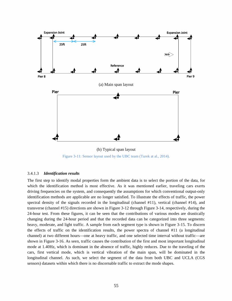
55

(a) Main span layout

(b) Typical span layout

Figure 3-11: Sensor layout used by the UBC team (Turek at al., 2014).

3.4.1.3 Identification results

The first step to identify modal properties form the ambient data is to select the portion of the data, for which the identification method is most effective. As it was mentioned earlier, traveling cars exerts driving frequencies on the system, and consequently the assumptions for which conventional output-only identification methods are applicable are no longer satisfied. To illustrate the effects of traffic, the power spectral density of the signals recorded in the longitudinal (channel #11), vertical (channel #14), and transverse (channel #15) directions are shown in Figure 3-12 through Figure 3-14, respectively, during the 24-hour test. From these figures, it can be seen that the contributions of various modes are drastically changing during the 24-hour period and that the recorded data can be categorized into three segments: heavy, moderate, and light traffic. A sample from each segment type is shown in Figure 3-15. To discern the effects of traffic on the identification results, the power spectra of channel #11 (a longitudinal channel) at two different hours—one at heavy traffic, and one selected time interval without traffic—are shown in Figure 3-16. As seen, traffic causes the contribution of the first and most important longitudinal mode at 1.40Hz, which is dominant in the absence of traffic, highly reduces. Due to the traveling of the cars, first vertical mode, which is vertical vibration of the main span, will be dominated in the longitudinal channel. As such, we select the segment of the data from both UBC and UCLA (CGS sensors) datasets within which there is no discernable traffic to extract the mode shapes.

56

Figure 3-12: Power spectra of longitudinal response signals recorded at channel #11 during 24hours am

bient tests.

00.5

11.5

2Frequancy (H

z)

Power Spectrum

00.5

11.5

2Frequancy (H

z)Power Spectrum

00.5

11.5

2Frequancy (H

z)

Power Spectrum

00.5

11.5

2Frequancy (H

z)

Power Spectrum

00.5

11.5

2Frequancy (H

z)

Power Spectrum

00.5

11.5

2Frequancy (H

z)

Power Spectrum

00.5

11.5

2Frequancy (H

z)

Power Spectrum

00.5

11.5

2Frequancy (H

z)

Power Spectrum

00.5

11.5

2Frequancy (H

z)

Power Spectrum

00.5

11.5

2Frequancy (H

z)

Power Spectrum

00.5

11.5

2Frequancy (H

z)

Power Spectrum

00.5

11.5

2Frequancy (H

z)

Power Spectrum

00.5

11.5

2Frequancy (H

z)

Power Spectrum

00.5

11.5

2Frequancy (H

z)

Power Spectrum

00.5

11.5

2Frequancy (H

z)

Power Spectrum

00.5

11.5

2Frequancy (H

z)

Power Spectrum

00.5

11.5

2Frequancy (H

z)

Power Spectrum

00.5

11.5

2Frequancy (H

z)

Power Spectrum

00.5

11.5

2Frequancy (H

z)

Power Spectrum

00.5

11.5

2Frequancy (H

z)

Power Spectrum

00.5

11.5

2Frequancy (H

z)

Power Spectrum

00.5

11.5

2Frequancy (H

z)

Power Spectrum

00.5

11.5

2Frequancy (H

z)

Power Spectrum

00.5

11.5

2Frequancy (H

z)

Power Spectrum

57

Figure 3-13: Power spectra of vertical response signals recorded at channel #14 during 24hours am

bient tests.

00.5

11.5

2Frequancy (H

z)

Power Spectrum

00.5

11.5

2Frequancy (H

z)Power Spectrum

00.5

11.5

2Frequancy (H

z)

Power Spectrum

00.5

11.5

2Frequancy (H

z)

Power Spectrum

00.5

11.5

2Frequancy (H

z)

Power Spectrum

00.5

11.5

2Frequancy (H

z)

Power Spectrum

00.5

11.5

2Frequancy (H

z)

Power Spectrum

00.5

11.5

2Frequancy (H

z)

Power Spectrum

00.5

11.5

2Frequancy (H

z)

Power Spectrum

00.5

11.5

2Frequancy (H

z)

Power Spectrum

00.5

11.5

2Frequancy (H

z)

Power Spectrum

00.5

11.5

2Frequancy (H

z)

Power Spectrum

00.5

11.5

2Frequancy (H

z)

Power Spectrum

00.5

11.5

2Frequancy (H

z)

Power Spectrum

00.5

11.5

2Frequancy (H

z)

Power Spectrum

00.5

11.5

2Frequancy (H

z)

Power Spectrum

00.5

11.5

2Frequancy (H

z)

Power Spectrum

00.5

11.5

2Frequancy (H

z)

Power Spectrum

00.5

11.5

2Frequancy (H

z)

Power Spectrum

00.5

11.5

2Frequancy (H

z)

Power Spectrum

00.5

11.5

2Frequancy (H

z)

Power Spectrum

00.5

11.5

2Frequancy (H

z)

Power Spectrum

00.5

11.5

2Frequancy (H

z)

Power Spectrum

00.5

11.5

2Frequancy (H

z)

Power Spectrum

58

Figure 3-14: Power spectra of transverse response signals recorded at channel #15 during 24hours am

bient tests.

00.5

11.5

2Frequancy (H

z)

Power Spectrum

00.5

11.5

2Frequancy (H

z)Power Spectrum

00.5

11.5

2Frequancy (H

z)

Power Spectrum

00.5

11.5

2Frequancy (H

z)

Power Spectrum

00.5

11.5

2Frequancy (H

z)

Power Spectrum

00.5

11.5

2Frequancy (H

z)

Power Spectrum

00.5

11.5

2Frequancy (H

z)

Power Spectrum

00.5

11.5

2Frequancy (H

z)

Power Spectrum

00.5

11.5

2Frequancy (H

z)

Power Spectrum

00.5

11.5

2Frequancy (H

z)

Power Spectrum

00.5

11.5

2Frequancy (H

z)

Power Spectrum

00.5

11.5

2Frequancy (H

z)

Power Spectrum

00.5

11.5

2Frequancy (H

z)

Power Spectrum

00.5

11.5

2Frequancy (H

z)

Power Spectrum

00.5

11.5

2Frequancy (H

z)

Power Spectrum

00.5

11.5

2Frequancy (H

z)

Power Spectrum

00.5

11.5

2Frequancy (H

z)

Power Spectrum

00.5

11.5

2Frequancy (H

z)

Power Spectrum

00.5

11.5

2Frequancy (H

z)

Power Spectrum

00.5

11.5

2Frequancy (H

z)

Power Spectrum

00.5

11.5

2Frequancy (H

z)

Power Spectrum

00.5

11.5

2Frequancy (H

z)

Power Spectrum

00.5

11.5

2Frequancy (H

z)

Power Spectrum

00.5

11.5

2Frequancy (H

z)

Power Spectrum

59

(a) heavy traffic

(b) moderate traffic

(c) light traffic

Figure 3-15: Accelerations recorded at Channel #14 on June 07 during three hours under different traffic loads.

0 10 20 30 40 50 60

0

x 10-18

Time (min.)

0 10 20 30 40 50 60

0

x 10-18

Time (min.)

0 10 20 30 40 50 60

0

x 10-18

Time (min.)

60

Figure 3-16: Power spectra of accelerations recorded at Channel #11 on June 07 under different traffic loads.

To identify natural frequencies and mode shapes from both UBC and UCLA datasets, our PARAFAC-based method (§3.2) is employed. To construct the correlation tensor, correlation matrices introduced in Eq. (5) are calculated at 5000 successive lags. Before calculating the correlation matrices, response signals are windowed by a Gaussian window proposed by McNeill and Zimmerman (2008). Also, the signals are replaced with their correlations with respect to all measured points at each setup (for UBC data), and then all matrices at all lags are used to construct the correlation tensor and in the decompositions. Finally, the results of each mode are chosen based the maximum deformation of the reference mode at that mode. As the UCLA data are collected using a single and sparse instrumentation setup, the results obtained from UBC datasets are considered as references. Table 3-3 to Table 3-5 presents the natural frequencies of the sources identified using the PARAFAC method in transverse, longitudinal, and vertical directions, respectively. As seen, because of existence of many local modes, some modes are only identified from specific setups. Moreover, values of the natural frequencies vary from setup to setup, because of identification errors or because of natural variations in the system properties with respect to time of day. However, the said variations due to inherent/natural variations (temperature, humidity, etc.) cannot be explicitly calculated here as the variations are not too large. By the same token, these effects will be ignored here.

Although many modes have been reported in Table 3-3 to Table 3-5, only a select few are reliable, because the number of sensors is limited and thus it is not possible to identify higher mode shapes. Moreover, since only one common point has been considered as the reference point among all setups during the experiments (i.e., middle point of the main span) and for some of the modes, this reference point is a node, mode shapes from different setups cannot be accurately combined with each other. For example, the third transverse mode suffers from this problem, and the identified mode shape is likely inaccurate. Based on these limitations, we are only able to extract the first 6 transverse modes, the first 4 longitudinal modes, and the first vertical mode. These mode shapes are shown in Figure 3-17 to Figure 3-18 where the mode shapes identified from different sensor layouts are shown with different colors.

0 0.5 1 1.5 2Frequancy (Hz)

Pow

er S

pect

rum

Without TrafficHeavy Traffic

61

Figure 3-17: Identified transverse mode shapes using different sensor setups (modes 1 to 4).

S1 S2 S3 S4 S5 S6 S7 S8 S9 S10 S11 S12 S13 S14 S15 S16 S17 S18 S19 S20 S21-1

0

1

Setup 1Setup 2Setup 3Setup 4Setup 5Setup 6Setup 7Setup 8Setup 9Setup 10Setup 11Setup 12


0

1



0

1



0

1


62

Figure 3-22(cont.): Identified transverse mode shapes using different sensor setups (modes 5 and 6).

Figure 3-18: First identified vertical mode shape using different sensor setups.


0

1



0

1



0

1


63

Figure 3-19: Identified longitudinal mode shapes using different sensor setups (modes 1 to 4).


0

1



0

1



0

1



0

1


64

Table 3-3: Identified transverse natural frequencies from UBC ambient data at all 12 setups using the PARAFAC technique.

Setup No. 1 2 3 4 5 6 7 8 9 10 11 12 M

ode

No.

1 1.05 1.00 1.00 1.00 0.97 -- 0.97 1.00 1.02 1.00 1.02 1.02 2 1.18 1.18 1.15 1.15 1.18 -- 1.15 1.18 1.18 1.20 1.18 1.18 3 1.36 1.33 -- 1.31 1.31 -- -- 1.36 1.33 1.36 -- 1.33 4 -- 1.48 -- -- -- 1.48 -- 1.46 1.48 1.48 1.51 1.48 5 1.59 1.61 1.61 -- -- -- -- -- -- -- -- 1.59 6 -- 1.72 1.74 1.77 1.74 -- -- 1.77 -- -- 1.77 1.77 7 -- -- 1.87 -- 1.79 -- -- 1.89 -- 1.82 -- 1.89 8 2.10 -- -- -- -- -- -- -- -- 2.12 1.97 -- 9 -- -- -- -- -- -- -- -- -- -- -- 2.25

10 -- -- 2.56 2.59 2.61 -- 2.56 -- 2.61 -- -- -- 11 -- -- 2.76 2.84 2.82 2.84 -- -- -- -- 2.76 2.82 12 -- -- -- -- -- -- -- -- -- 3.30 -- -- 13 -- -- -- 3.53 -- -- -- -- -- -- -- -- 14 5.09 5.07 5.07 5.04 -- -- 4.86 -- -- 4.89 -- --

Table 3-4: Identified longitudinal natural frequencies from UBC ambient data at all 12 setups using the PARAFAC technique.

Setup No. 1 2 3 4 5 6 7 8 9 10 11 12

Mod

e N

o. 1 1.36 1.38 1.43 1.36 -- 1.46 1.38 1.38 -- 1.46 1.46 1.38

2 3.02 -- -- -- -- 3.07 -- -- -- -- -- 3.17 3 -- -- 3.94 3.94 -- 4.07 4.04 -- 4.02 -- 3.92 -- 4 -- -- -- -- -- 5.40 5.43 -- -- -- 5.43 5.43

Table 3-5: Identified vertical natural frequencies from UBC ambient data at all 12 setups using the PARAFAC technique.

Setup No. 1 2 3 4 5 6 7 8 9 10 11 12

Mode No. 1 1.79 1.69 1.74 1.77 1.79 1.82 -- 1.82 1.87 1.82 1.82 --

The natural frequencies reported in the previous tables have been identified from the modal coordinates’ auto-correlations, which are recovered during the PARAFAC decomposition. As representative examples, the recovered modal coordinates and their Fourier spectra for some selected modes are shown in Figure 3-20 to Figure 3-22 for transverse, longitudinal, and vertical modes. As seen, the recovered signals are very near to being pure mono-component signals.

65

Figure 3-20: Windowed modal coordinates’ auto-correlation signals recovered from UBC ambient data in the

transverse direction using the PARAFAC technique: Mode 1 (top), Mode 5 (mid), and Mode 6 (bot).

0 5 10 15 20 25 30 35 40

0

Time (sec.)0 1 2 3 4 5 6

Frequency (Hz)

0 5 10 15 20 25 30 35 40

0

Time (sec.)0 1 2 3 4 5 6

Frequency (Hz)

0 5 10 15 20 25 30 35 40

0

Time (sec.)0 1 2 3 4 5 6

Frequency (Hz)

66

Figure 3-21: Windowed modal coordinates’ auto-correlation signals recovered from UBC ambient data in the

longitudinal direction using the PARAFAC technique: Mode 1 (top), Mode 2 (mid), and Mode 4 (bot).

0 5 10 15 20 25 30 35 40

0

Time (sec.)0 1 2 3 4 5 6

Frequency (Hz)

0 5 10 15 20 25 30 35 40

0

Time (sec.)0 1 2 3 4 5 6

Frequency (Hz)

0 5 10 15 20 25 30 35 40

0

Time (sec.)0 1 2 3 4 5 6

Frequency (Hz)

67

Figure 3-22: Windowed first modal coordinate’s auto-correlation recovered from UBC ambient data in the vertical

direction using the PARAFAC technique.

To verify the identified results, the Frequency Domain Decomposition (FDD) method (Brincker et al., 2001) as another output-only identification method, which is extensively used in well-known identification software, such as ARTEMIS (2013), is employed. In the FDD method, the dominant peaks at the largest singular values of the average cross-power spectral densities of the response signals are detected as modes. For calculating the average cross-power spectral densities, Welch’s (1967) averaged modified periodogram method has been used. In this method, the signals are divided into several segments by a specific overlap and the average spectra are calculated. Here, we divide the data using a Hamming window with a 30-second length and 50% overlap. Figure 3-23 to Figure 3-25 show the three largest singular values, where in the natural frequencies are clearly detected in the first largest singular values’ curves (black curves).

Table 3-6 to Table 3-8 present the identified natural frequencies using FDD method. As seen, these values are very close to those identified through the PARAFAC method. In Table 3-9, the mean value of the natural frequencies identified by two methods from different setups along with their standard deviations are shown, which shows that results identified from two different methods are very similar. Finally, the reliable mode shapes, which are identified from the two methods, are compared through the MAC index in Table 3-10. Again, it is seen that the mode shapes from both methods are very similar, except the last transverse mode and the two last longitudinal modes, where some discrepancies are observed.

0 5 10 15 20 25 30 35 40

0

Time (sec.)0 1 2 3 4 5 6

Frequency (Hz)

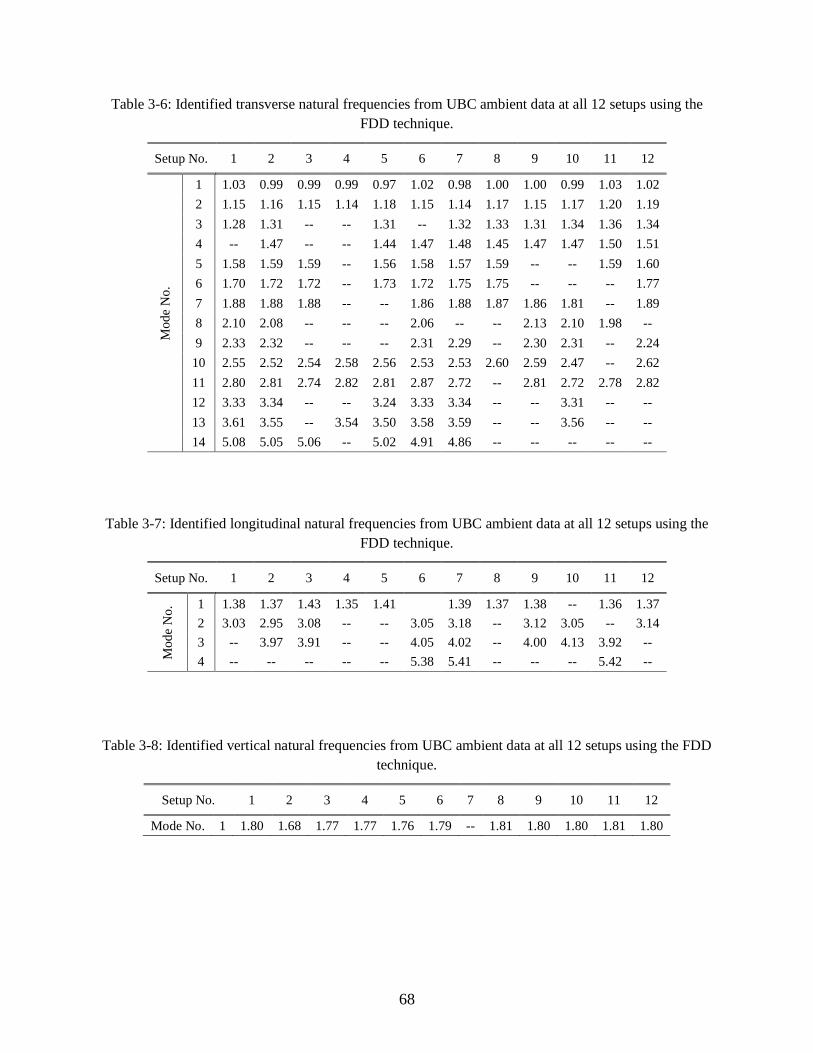
68

Table 3-6: Identified transverse natural frequencies from UBC ambient data at all 12 setups using the FDD technique.

Setup No. 1 2 3 4 5 6 7 8 9 10 11 12 M

ode

No.

1 1.03 0.99 0.99 0.99 0.97 1.02 0.98 1.00 1.00 0.99 1.03 1.02 2 1.15 1.16 1.15 1.14 1.18 1.15 1.14 1.17 1.15 1.17 1.20 1.19 3 1.28 1.31 -- -- 1.31 -- 1.32 1.33 1.31 1.34 1.36 1.34 4 -- 1.47 -- -- 1.44 1.47 1.48 1.45 1.47 1.47 1.50 1.51 5 1.58 1.59 1.59 -- 1.56 1.58 1.57 1.59 -- -- 1.59 1.60 6 1.70 1.72 1.72 -- 1.73 1.72 1.75 1.75 -- -- -- 1.77 7 1.88 1.88 1.88 -- -- 1.86 1.88 1.87 1.86 1.81 -- 1.89 8 2.10 2.08 -- -- -- 2.06 -- -- 2.13 2.10 1.98 -- 9 2.33 2.32 -- -- -- 2.31 2.29 -- 2.30 2.31 -- 2.24

10 2.55 2.52 2.54 2.58 2.56 2.53 2.53 2.60 2.59 2.47 -- 2.62 11 2.80 2.81 2.74 2.82 2.81 2.87 2.72 -- 2.81 2.72 2.78 2.82 12 3.33 3.34 -- -- 3.24 3.33 3.34 -- -- 3.31 -- -- 13 3.61 3.55 -- 3.54 3.50 3.58 3.59 -- -- 3.56 -- -- 14 5.08 5.05 5.06 -- 5.02 4.91 4.86 -- -- -- -- --

Table 3-7: Identified longitudinal natural frequencies from UBC ambient data at all 12 setups using the FDD technique.

Setup No. 1 2 3 4 5 6 7 8 9 10 11 12

Mod

e N

o. 1 1.38 1.37 1.43 1.35 1.41 1.39 1.37 1.38 -- 1.36 1.37

2 3.03 2.95 3.08 -- -- 3.05 3.18 -- 3.12 3.05 -- 3.14 3 -- 3.97 3.91 -- -- 4.05 4.02 -- 4.00 4.13 3.92 -- 4 -- -- -- -- -- 5.38 5.41 -- -- -- 5.42 --

Table 3-8: Identified vertical natural frequencies from UBC ambient data at all 12 setups using the FDD technique.

Setup No. 1 2 3 4 5 6 7 8 9 10 11 12

Mode No. 1 1.80 1.68 1.77 1.77 1.76 1.79 -- 1.81 1.80 1.80 1.81 1.80

69

Table 3-9: Summary of the identified natural frequencies from UBC ambient data using the FDD and PARAFAC techniques.

FDD PARAFAC

Mode No. Mean StD mean StD

Transverse

1 1.00 0.02 1.00 0.02 2 1.16 0.02 1.17 0.02 3 1.32 0.02 1.34 0.02 4 1.47 0.02 1.48 0.01 5 1.58 0.01 1.6 0.01 6 1.73 0.02 1.75 0.02 7 1.87 0.02 1.85 0.04 8 2.08 0.05 2.06 0.08 9 2.3 0.03 2.25 --

10 2.55 0.04 2.59 0.03 11 2.79 0.05 2.81 0.04 12 3.3 0.04 3.3 -- 13 3.56 0.04 3.53 -- 14 5.00 0.09 5.00 0.10

Longitudinal

1 1.38 0.02 1.41 0.04 2 3.08 0.07 3.09 0.08 3 4.00 0.08 3.99 0.06 4 5.40 0.02 5.42 0.02

Vertical 1 1.78 0.04 1.79 0.05

Table 3-10: MAC indices between mode shapes identified from UBC data using the FDD and PARAFAC techniques.

Transverse Longitudinal Vertical

Mode No. 1 2 3 4 5 6 1 2 3 4 1

MAC 1.00 0.98 0.96 0.96 0.95 0.84 1.00 0.93 0.79 0.87 0.99

70

Figure 3-23: Average spectra for the largest SVD values of the UBC data in the transverse direction for all 12

different setups.

0 1 2 3 4 5 6Frequency (Hz)












71

Figure 3-24: Average spectra for the largest SVD values of the UBC data in longitudinal direction for all 12

different setups.













72

Figure 3-25: Average spectra for the largest SVD values of the UBC data in the vertical direction for all 12 different

setups.

By applying the same approach described above to the UCLA data, natural frequencies of the first six transverse modes as well as the first four longitudinal modes are identified. Vertical modes cannot be identified, because in this case, we have only one sensor in the vertical direction. Averages of the identified frequencies using the FDD and PARAFAC methods are shown in Table 3-11. By comparing these values with those already presented in Table 3-9, it can be seen that we can get the same results from two datasets (a small error is observed in the third longitudinal mode identified from UCLA data). However, if we did not have the UBC data, it would be very difficult to distinguish between modes using













73

their mode shapes identified from UCLA data due to instrumentation sparsely in the latter case. Figure 3-26 and Figure 3-27 display the first longitudinal and six transverse mode shapes identified from UCLA data (red circles9) plotted on mode shape curves obtained from the UBC data. As seen, only the first and third transverse mode shapes can be constructed by the current CSMIP instrumentation, which clearly shows the inadequacy of the current instrumentation density.

The final set of results is the set of identified damping ratios. We estimated the damping ratios from the UBC data through the identified modal coordinates’ auto-correlations recovered during the PARAFAC decomposition. Note that the recovered signals are windowed versions of the original auto-correlations, and must be treated properly to remove windowing effects, as described by Abazarsa et al. (2013b). After this step, the auto-correlation signals are in the form of exponentially decaying sinusoids whose decay rates are −𝜔𝑛𝜉 (see, for example, Yang et al., 2003) with 𝜔𝑛 and 𝜉 denoting, respectively, natural frequency and damping ratio of the mode. So, the slope of the natural logarithm of the instantaneous amplitudes of the recovered modal coordinates’ auto-correlations divided by ωn is – ξ. Figure 3-28 shows this approach for the first transverse mode and Table 3-12 presents the estimated damping ratios for the other modes. In this table, only the reliable values are shown.

Table 3-11: Natural frequencies identified from UCLA data (averages of FDD and PARAFAC methods).

Mode No. 1 2 3 4 5 6

Transverse 1.02 1.17 1.33 1.48 1.57 1.72

Longitudinal 1.40 3.07 3.82 5.40 --- ---

Table 3-12: Identified damping ratios (%) from UBC data using the PARAFAC technique.

Mode No. 1 2 3 4 5 6

Transverse 0.4 0.7 0.4 0.7 1.0 1.0

Longitudinal 0.8 --- --- --- --- ---

Vertical 0.8 --- --- --- --- ---

9 As will be shown later, channel 18 of CGS had a problem and did not work during ambient testing. For this reason, we do not have a data point (a red marker) on S14.

74

Figure 3-26: Comparison of transverse mode shapes identified from UBC and CGS sensors.

Figure 3-27: Comparison of longitudinal mode shapes identified from UBC and CGS sensors.

Figure 3-28: A sample of damping ratios estimation from natural logarithm of the instantaneous amplitude of the

first transverse mode’s auto-correlation.


0

1

UBC

CGS


0

1

UBC

CGS


0

1

UBC

CGS


0

1

UBC

CGS


0

1

UBC

CGS


0

1

UBC

CGS


0

1

UBC

CGS

0 10 20 30 40-0.3

-0.2

-0.1

0

Time (sec.)

Fit: y = - 0.004 * t - 0.04

75

3.4.2 Earthquake data To start identification of the modal properties from earthquake-induced response signals through the previously introduced blind identification method (§3.3), it is necessary to decide which part of the signals must be used. Figure 3-29 presents the time history and Fourier spectra of two signals recorded during the 2007 Ferndale earthquake. In this figure, each signal is divided into two segments with different amplitude orders. The first part shows that the first 21 seconds of the earthquake contain very small vibrations mostly produced by primary waves, while the second part contains vibrations with large amplitudes. As this figure shows, dominant frequencies do not change significantly from the first to the second part during this weak earthquake (note that Fourier spectra are normalized so that both parts have the same maximum amplitude). Such a pattern was also observed in other weak earthquakes—namely, Trinidad 2007, Willow Creek 2008, and Trinidad 2008. Here, we use only the second portions of the data—which are the more important parts—to identify the modal properties from earthquake signals.

Figure 3-29: Time variation of the longitudinal (top) and transverse (bottom) natural frequencies of the bridge

during Ferndale earthquake, 2007.

Unlike the weak earthquakes, data recorded during the 2010 Ferndale earthquake exhibits three distinct portions. As it can be seen in Figure 3-30, the first 28 seconds of the data contains vibration produced mainly by ambient-type excitations, which are followed by low-amplitude primary waves. During this

76

segment, natural frequencies of the system along both directions are similar to those identified from ambient test data, and thus will not be discussed again here. In the second part, which is the main shock of the earthquake, vibrations with large amplitudes are seen. As the Fourier spectra of the middle portions show, natural frequencies have significantly dropped during the main shock. At the last 34 seconds, small amplitude free vibrations are observed during which natural frequencies are slightly recovered, but not to their initial values.

Figure 3-30: Time variation of the longitudinal (top) and transverse (bottom) natural frequencies of the bridge

during Ferndale earthquake, 2010.

To visualize the frequency variations as they occur, time-frequency representations of the recorded data can be employed. Figure 3-31 displays the SMoothed Wigner-Ville Distribution (SMWVD) (Flandrin, 1999) of the signal recorded at channel #6. As the energy of the signal is very concentrated in time, the basic/nominal time-frequency representation of the original signal cannot display the time-variation of the frequencies clearly. To solve this problem, we have synthetically scaled the signal by its instantaneous amplitude10. As Figure 3-31 shows, first longitudinal natural frequency is about 0.81Hz at 30 seconds after start time and rapidly drops to 0.68Hz and remains constant for at least 10 seconds. Finally, it

10 A definition of instantaneous amplitude may be found in Yang et al. (2003).

77

recovers at the last times of the earthquake. To see this with much better time-resolution, the first 28 seconds is removed from Figure 3-31 and the resulting plot is shown in Figure 3-32. Time-variation of the longitudinal natural frequency is clearly seen in this figure.

Similar to Figure 3-32, Figure 3-33 displays time-frequency representation of channel #10. As it can be seen in this figure, in the time interval between 40 to 50 seconds, system has its minimum natural frequency in the transverse direction. Then, natural frequency is recovering from its minimum, i.e., 0.66 Hz, to larger values gradually. Two points must be considered when this figure is compared to its counterpart for the longitudinal directions. First, the frequency reduction is not visible at the beginning times of the figure, because the signal is polluted by high-frequency components that control the instantaneous amplitudes. So, by scaling the signal by instantaneous amplitude, this section will have very small amplitude/energy in the frequency range around the first transverse natural frequency. Second, Figure 3-33 is drawn to the end of the signal’s duration, because we have relatively large amplitudes free vibrations. On account of these observations, the second part of the Ferndale earthquake 2010 is used in this chapter as the representative of a severe earthquake.

In the following subsections, details of the identification procedures are presented only for two earthquake data sets—namely, 2007 Ferndale and 2008 Willow Creek earthquakes—for brevity. For other earthquakes, only the final results are provided.

Figure 3-31: Time-frequency representation of channel #6 during the 2010 Ferndale earthquake.

0

Signal in time

Ene

rgy

spec

tral d

ensi

ty

Time (Sec.)

Freq

uenc

y (H

z)

0 10 20 30 40 50 60 700.5

0.6

0.7

0.8

0.9

1

0.67 Hz

0.71 Hz

0.81 Hz

78

Figure 3-32: Time-frequency representation of channel #6 during the 2010 Ferndale earthquake for the time interval

[28-75] seconds.

Figure 3-33: Time-frequency representation of channel #10 during the 2010 Ferndale earthquake for the time

interval [28-90] seconds.

0

Signal in time

Ener

gy s

pect

ral d

ensi

ty

Time (Sec.)

Freq

uenc

y (H

z)

30 40 50 60 700.5

0.6

0.7

0.8

0.9

1

0.81 Hz

0.71 Hz

0.67 Hz

0

Signal in time

Ener

gy s

pect

ral d

ensi

ty

Time (Sec.)

Freq

uenc

y (H

z)

30 40 50 60 70 80 900.5

0.6

0.7

0.8

0.9

1

0.82 Hz

0.66 Hz

0.77 Hz

79

3.4.2.1 Modal identification using earthquake data Unlike the ambient case, we have a limited number of sensors that recorded the response of the bridge during earthquakes. This limitation will naturally reduce the accuracy of the identification results. As an illustration, consider Figure 3-34, which shows the MAC indices among the transverse mode shapes identified from ambient data. As seen, all of these modes are almost independent (MAC values are lower than 0.1). Only the last two modes have a MAC index of ~0.4, because even the ambient instrumentation scenario cannot perfectly distinguish between these two mode shapes. If we reduce the measurement points to the current CSMIP sensors, then the MAC indices among these 6 identified mode shapes become those values shown in Figure 3-35, which are far greater than those in the previous figure. Especially, the first and the second mode shapes are become very similar when only the CGS sensors are employed. Therefore, we do not expect to be able to identify the second mode accurately from earthquake data. It is important to note that the mode shapes will be different during earthquakes rather than ambient, so the similarities among mode shapes at CGS sensors may increase in some other modes.

Figure 3-34: MAC indices among mode shapes identified from ambient data.

Figure 3-35: MAC indices among ambient mode shapes reduced at CGS instrumented points.

Mode No.

Mod

e N

o.

1 2 3 4 5 6

1

2

3

4

5

6

0.2

0.4

0.6

0.8

1

Mode No.

Mod

e N

o.

1 2 3 4 5 6

1

2

3

4

5

6

0.2

0.4

0.6

0.8

1

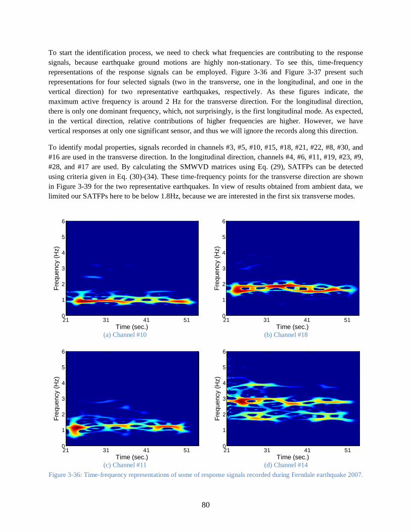
80

To start the identification process, we need to check what frequencies are contributing to the response signals, because earthquake ground motions are highly non-stationary. To see this, time-frequency representations of the response signals can be employed. Figure 3-36 and Figure 3-37 present such representations for four selected signals (two in the transverse, one in the longitudinal, and one in the vertical direction) for two representative earthquakes, respectively. As these figures indicate, the maximum active frequency is around 2 Hz for the transverse direction. For the longitudinal direction, there is only one dominant frequency, which, not surprisingly, is the first longitudinal mode. As expected, in the vertical direction, relative contributions of higher frequencies are higher. However, we have vertical responses at only one significant sensor, and thus we will ignore the records along this direction.

To identify modal properties, signals recorded in channels #3, #5, #10, #15, #18, #21, #22, #8, #30, and #16 are used in the transverse direction. In the longitudinal direction, channels #4, #6, #11, #19, #23, #9, #28, and #17 are used. By calculating the SMWVD matrices using Eq. (29), SATFPs can be detected using criteria given in Eq. (30)-(34). These time-frequency points for the transverse direction are shown in Figure 3-39 for the two representative earthquakes. In view of results obtained from ambient data, we limited our SATFPs here to be below 1.8Hz, because we are interested in the first six transverse modes.

(a) Channel #10 (b) Channel #18

(c) Channel #11 (d) Channel #14

Figure 3-36: Time-frequency representations of some of response signals recorded during Ferndale earthquake 2007.

Time (sec.)

Freq

uenc

y (H

z)

21 31 41 510

1

2

3

4

5

6

Time (sec.)

Freq

uenc

y (H

z)

21 31 41 510

1

2

3

4

5

6

Time (sec.)

Freq

uenc

y (H

z)

21 31 41 510

1

2

3

4

5

6

Time (sec.)

Freq

uenc

y (H

z)

21 31 41 510

1

2

3

4

5

6

81

(a) Channel #10 (b) Channel #18

(c) Channel #11 (d) Channel #14

Figure 3-37: Time-frequency representations of some of response signals recorded during Willow Creek earthquake 2008.

Figure 3-38: SATFPs found from Ferndale earthquake,

2007. Figure 3-39: SATFPs found from Willow Creek

earthquake, 2008.

Time (sec.)

Freq

uenc

y (H

z)

14 24 34 44 540

1

2

3

4

5

6

Time (sec.)

Freq

uenc

y (H

z)

14 24 34 44 540

1

2

3

4

5

6

Time (sec.)

Freq

uenc

y (H

z)

14 24 34 44 540

1

2

3

4

5

6

Time (sec.)

Freq

uenc

y (H

z)

14 24 34 44 540

1

2

3

4

5

6

82

One of the important parameters in any identification problem is the model order. In the proposed blind identification, the number of “sources” plays this role. According to the Table 3-1, using 10 signals it is possible to extract at most 41 sources. Therefore, PARAFAC decomposition is employed by assuming a range of sources from 1 to 41 first. Then, by using stability diagrams (Bodeux and Golinval, 2001), the most appropriate source number is detected using the following criteria:

Δ𝑓/𝑓 < 1% (36)

MAC > 0.90 (37)

Figure 3-41 shows the stability diagrams for the transverse direction. For the Ferndale earthquake (2007), the second mode was not detected as it can be seen in the corresponding stability diagram. The first stable results are obtained by using a source number of 29. For the Willow Creek earthquake (2008), the most appropriate selection for the number of sources is 31.

By removing similar identified mode shapes through MAC indices, the mode shapes are identified as shown in Figure 3-42 and Figure 3-43, for the Ferndale and Willow Creek earthquakes, respectively. In these figures, the mode shapes identified from ambient test data are also shown by solid lines. As seen, modal deformations of the instrumented points during earthquakes (i.e., the red circles) generally follow the ambient mode shapes in the lower modes, but large deviations are observed in the higher modes.

Figure 3-40: Stability diagram for the Ferndale earthquake 2007.

0.5 0.8 1.1 1.4 1.7 2

10

20

30

40

Frequency (Hz)

Sour

ce N

o.

83

Figure 3-41: Stability diagram for the Willow Creek earthquake 2008.

After identifying the mode shapes, we employ the subspace approach suggested by Ghahari et al. (2013c) to recover modal coordinates’ auto-WVD. Upper part of the Figure 3-44 and Figure 3-45 show these time-frequency plots for two representative earthquakes for three transverse modes. Consequently, the natural frequency of each mode can be obtained as the frequency corresponding to the maximum value of the index E(f) introduced in Eq. (35). The frequency variations of this index for the three modes are shown in the bottom part of the Figure 3-44 and Figure 3-45, in which natural frequencies are shown by the vertical red lines.

0.5 0.8 1.1 1.4 1.7 2

10

20

30

40

Frequency (Hz)

Sour

ce N

o.

84

Figure 3-42: Comparison of mode shapes identified from ambient and Ferndale earthquake 2007. Top to bottom:

First, third and fourth transverse modes.


0

1

Ambient

Earthquake


0

1

Ambient

Earthquake


0

1

Ambient

Earthquake

85

Figure 3-42 (cont.): Comparison of mode shapes identified from ambient and Ferndale earthquake 2007. Fifth (top)

and sixth (bottom) transverse modes.


0

1

Ambient

Earthquake


0

1

Ambient

Earthquake

86

Figure 3-43: Comparison of mode shapes identified from ambient and Willow Creek earthquake 2008. Top to

bottom: First, second and third transverse modes.


0

1

Ambient

Earthquake


0

1

Ambient

Earthquake


0

1

Ambient

Earthquake

87

Figure 3-43 (cont.): Comparison of mode shapes identified from ambient and Willow Creek earthquake 2008. Top

to bottom: fourth, fifth and sixth transverse modes.


0

1

Ambient

Earthquake


0

1

Ambient

Earthquake


0

1

Ambient

Earthquake

88

(a) First mode (b) Third mode (c) Sixth mode

Figure 3-44: Recovered time-frequency representations of the modal coordinates (top), and identified natural frequencies (bottom) for Ferndale earthquake, 2007.

(a) First mode (b) Third mode (c) Sixth mode

Figure 3-45: Recovered time-frequency representations of the modal coordinates (top), and identified natural frequencies (bottom) for Willow Creek earthquake, 2008.

The identified natural frequencies of the bridge in the transverse direction for the two representative earthquakes are tabulated in Table 3-13 and Table 3-14. In these tables, natural frequencies identified from ambient test data are also shown for comparison. The frequency errors (assuming ambient values as references) show that the system exhibits different stiffnesses during the earthquakes compared to the

Time (sec.)

Freq

uenc

y (H

z)

21 31 41 510

0.3

0.6

0.9

1.2

1.5

1.8

Time (sec.)

21 31 41 510

0.3

0.6

0.9

1.2

1.5

1.8

Time (sec.)

21 31 41 510

0.3

0.6

0.9

1.2

1.5

1.8

0.7 0.8 0.9 1 1.10

2

4

6

8

10

Frequency (Hz)

Ener

gy (%

)

1 1.1 1.2 1.3 1.40

2

4

6

8

Frequency (Hz)

gy (

)

1.5 1.6 1.70

2

4

6

8

10

Frequency (Hz)

Time (sec.)

Freq

uenc

y (H

z)

14 24 34 44 540

0.3

0.6

0.9

1.2

1.5

1.8

Time (sec.)

14 24 34 44 540

0.3

0.6

0.9

1.2

1.5

1.8

Time (sec.)

24 34 44 54

0.3

0.6

0.9

1.2

1.5

1.8

0.7 0.8 0.9 1 1.10

2

4

6

8

10

Frequency (Hz)

Ene

rgy

(%)

1 1.1 1.2 1.30

2

4

6

8

10

Frequency (Hz)

1.4 1.5 1.6 1.70

2

4

6

Frequency (Hz)

89

ambient case. In the last column of these tables, MAC indices calculated between mode shapes identified from earthquake and ambient data are shown. As seen, in the lower modes, they are very similar to each other, but in the higher modes they are quite different.

Table 3-13: Comparison of modal properties identified from ambient tests and 2007 Ferndale earthquake.

Mode No. Frequency (Hz)

MAC (%) Earthquake Ambient Error (%)

Transverse

1 0.92 1 8.70 0.99 2 --- 1.16 --- --- 3 1.18 1.33 11.28 0.83 4 1.33 1.48 10.14 0.57 5 1.52 1.60 5.00 0.68 6 1.61 1.74 7.47 0.86

Table 3-14: Comparison of modal properties identified from ambient tests and 2008 Willow Creek earthquake.


MAC (%) Earthquake Ambient Error (%)

Transverse

1 0.91 1 9.00 0.97 2 1.10 1.16 5.17 0.84 3 1.14 1.33 14.29 0.89 4 1.30 1.48 12.16 0.61 5 1.47 1.60 8.13 0.67 6 1.55 1.74 10.92 0.36

For the longitudinal direction, we present the details for the 2007 Ferndale earthquake, because we could not extract reliable results from the 2008 Willow Creek earthquake11. For other earthquakes, we present only the final results.

Figure 3-46 displays the SATPs selected by the criteria using SMWVD matrices calculated using channels #4, #6, #11, #19, #23, #9, #28, and #17. As we were interested in the first mode, we selected a very small value for the ϵGrad (0.001). As it can be seen, a very limited number of points are selected. Then, PARAFAC decomposition is employed by assuming a range of sources from 1 to 26 according to the Table 3-1. The first longitudinal mode was selected using the stability diagrams described earlier. Figure 3-47 displays the identified mode shape with red circles over the mode shape already extracted from ambient test data. As seen, the two mode shapes are similar, although not identical, at these CSMIP instrumentation points.

11 Preliminary results obtained from spectral analyses (see, Table 2-3) exhibited the same problem.

90

Figure 3-46: SATFPs obtained for longitudinal direction data through the proposed selection criterion.

Figure 3-47: Comparison of the first longitudinal mode shape identified from ambient test and the 2007 Ferndale earthquake.

In similar fashion to the transverse direction, time-frequency points of the first longitudinal mode is recovered with which the natural frequency can be estimated by calculating the energy index. The first

longitudinal frequency identified from all earthquake data are shown in

Table 3-15. In this table, natural frequencies of the first six transverse modes are also presented. The last row of this table shows the natural frequencies identified from different earthquakes for the first vertical mode. Note that, for the vertical direction, there in only one sensor on the deck, and thus the use of any sophisticated identification technique would be moot. Instead, we use the basic peak-picking method to find the natural frequency of this mode from the signal recorded in channel #14.


0

1

Ambient

Earthquake

91

Figure 3-48: Recovered time-frequency representation of the first longitudinal modal coordinate (left), and its

natural frequency identification (right) (Ferndale earthquake, 2007).

Table 3-15: Identified natural frequencies (Hz) from different earthquakes.

Direction Mode No. Ferndale 2007

Trinidad 2007

Willow Creek 2008

Trinidad 2008

Ferndale 2010

Tran

sver

se

1 0.92 0.94 0.91 0.92 0.68

2 --- 1.02 1.10 1.06 0.77

3 1.18 1.14 1.14 1.12 0.86

4 1.33 1.30 1.30 1.27 0.98

5 1.52 1.49 1.47 1.44 1.02

6 1.61 1.57 1.55 1.57 1.13

Longitudinal 1 1.22 1.23 --- 1.23 0.67

Vertical 1 1.68 1.73 1.68 1.72 1.9212

12 Natural frequency of the bridge in the vertical direction has been significantly increased during this earthquake. The reason of such unusual behavior can be described by the existence of the gaps in the deck. During sever earthquake, these gaps is closed and the bending stiffness of the main span is increased.

Time (sec.)

Freq

uenc

y (H

z)

21 31 41 510

0.5

1

1.5

2

1 1.1 1.2 1.3 1.40

2

4

6

8

Frequency (Hz)

Ener

gy (%

)

93

Chapter 4 FINITE ELEMENT MODEL UPDATING AND RESPONSE PREDICTION

4.1. INTRODUCTION

The Finite Element method’s roots reach as far back to Hrennikoff (1941), and this method has evolved over the ensuing decades into being the primary tool of analysis and design in almost every engineering application. It goes without saying that the FE method produces only approximate solutions to problems devised using approximate models, and thus the FE model of a structure (bridge) does not always produce those responses measured on its real-life counterpart. Omitting measurement errors, the sources of said discrepancies can be categorized as follows (Friswell and Mottershead, 1995):

• Difficulties in modeling connections, boundaries, and damping; • Difficulties in modeling nonlinearities; • Difficulties in modeling material properties.

Finite element model updating is a method through which an initial FE model is modified so that it has minimum possible differences relative to the real-life measurements (Marwala, 2010). Generally, finite element model updating can be categorized into two types: direct and iterative. In the direct approach, the FE model is updated without considering the feasibility of the updated parameters. In the other words, direct approach tends to update the system—i.e., mass, stiffness, and damping—matrices of the FE model so that it can produce responses as close to the measured values as possible without any regard to the structure that is under study. Not surprisingly, this approach may yield system matrices that do not represent physics of the system and thus alternative, iterative, methods are usually preferred. In iterative techniques, physical parameters—e.g., modulus of elasticity—of the model are updated until the FE model can accurately mimic the measured responses. Using this approach, the structures of the system matrices are preserved, so the model keeps assumed physics of the real system intact. In this study, we adopt and iterative model updating methods so that results obtained for the Samoa Channel Bridge can be extended other, similar, bridges.

Before starting with the model updating processes, we should make sure if updating is actually needed, and if so, determine which parameters should be updated. As seen in Table 4-1, although the initial FE model is created using almost every detail available from structural drawings and geotechnical data13, its modal properties (henceforth referred to as analytical or model modal properties) are different from those identified using ambient test data. It is expedient to note here that the analytical modal properties reported in Table 4-1 are calculated 14 without considering concrete cracking effects; however, the analytical natural frequencies are smaller than the ambient values (in lower modes

Prior to any model updating, we assume that under the ambient conditions, the system behaves as a classically damped system, so the damping parameters will not affect the natural frequencies and mode shapes. Moreover, even without considering cracking effects, natural frequencies of the FE model are lower than the real values (in lower modes), so the observed discrepancies cannot be explained by

13 That is, the distribution of stiffness through the bridge, and its topology and connectivities are as accurately represented in the initial FE model as possible. 14 Let us note here that the longitudinal and vertical modes of the bridge are highly coupled, so it is not quite possible to extract the higher longitudinal modes from the FE model.

94

cracking effects. Consequently, of the three difficulties mentioned above, the most likely reason for the discrepancy observed here is that the boundaries might not have be modeled accurately—in other words, the soil springs must be modified.

Table 4-1: Comparison of modal properties calculated using FE and identified from ambient tests.


MAC (%) FE Identified Error (%)

Transverse

1 0.93 1 7.00 0.87 2 1.12 1.16 3.45 0.80 3 1.34 1.33 0.75 0.71 4 1.57 1.48 6.08 0.88 5 1.73 1.60 4.38 0.88 6 1.87 1.74 7.47 0.69

Longitudinal

1 1.32 1.40 5.71 0.95 2 -- 3.07 -- -- 3 -- 3.96 -- -- 4 -- 5.71 -- --

Vertical 1 1.65 1.78 7.30 0.91

4.2. REDUCING THE MODEL SIZE

The model updating procedure for the full Samoa Bridge model is very expensive computationally. This task can be significantly simplified by removing redundant elements to reduce the model’s complexities. To do so, we use the substructure method. That is, the soil-pile system at each pier (Figure 4-1(a)) is replaced by a 4 × 4 stiffness matrix (Figure 4-1(b)), and a new and simpler bridge model—as shown in Figure 4-1(c)—is produced. To estimate the stiffness matrix, the superstructure is removed from the finite element model and the stiffness matrix of each pier’s soil-pile system is calculated through a flexibility approach. As expected, among these ten stiffness parameters (at each pier), there are six significant values—namely, two stiffness parameters for horizontal translation, two stiffness parameters for rocking, and two coupling terms.

Table 4-2: Comparison of modal properties of direct and substructure FE models.

Mode No. Frequency

MAC (%) Direct Substructure Error (%)

Transverse

1 0.93 0.91 2.93 1.00 2 1.12 1.08 3.86 1.00 3 1.34 1.29 3.75 1.00 4 1.57 1.49 5.10 0.99 5 1.73 1.65 4.79 0.96 6 1.87 1.77 5.30 0.83

Longitudinal 1 1.32 1.26 4.70 1.00 Vertical 1 1.65 1.61 2.47 1.00

95

To make sure that the simplified model has the same modal properties as the original model, errors of the natural frequencies and the mode shapes’ similarity indices (i.e., MAC values) are presented in Table 4-2. As seen, modal properties of the simple (reduced-order) model—in which the nonlinear soil-pile springs are replaced by 4 × 4 stiffness matrices—are very close to those of the original model, especially for the lower modes, which are the most important modes. In Table 4-3, the modal properties of this simplified FE model are compared to the values identified from ambient test data.

Table 4-3: Comparison of modal properties calculated using simplified FE model and those identified from ambient tests.


MAC (%) Substructure Identified Error (%)

Transverse

1 0.91 1 9.00 0.89 2 1.08 1.16 6.90 0.82 3 1.29 1.33 3.01 0.72 4 1.49 1.48 0.01 0.90 5 1.65 1.60 3.13 0.83 6 1.77 1.74 1.72 0.81

Longitudinal

1 1.26 1.40 10.0 0.96 2 -- 3.07 -- -- 3 -- 3.96 -- -- 4 -- 5.71 -- --

Vertical 1 1.61 1.78 9.55 0.93

(a) (b)

(c) Figure 4-1: Samoa Channel Bridge: (a) a typical soil-pile system, (b) its 4 × 4 stiffness matrix replacement, and (c)

the reduced FE model.

96

4.3. SENSITIVITY ANALYSES WITH UPDATING PARAMETERS

An objective function will be devised later to measure the discrepancy between the modal properties (i.e., natural frequencies and mode shapes) identified from real-life data and those computed using the FE mode, and will be minimized during the model updating procedure. For the Samoa Channel Bridge, consideration of all non-zero parameters of the stiffness matrices, as well as two lateral and longitudinal stiffnesses at both abutments results in a total of 118 model-updating parameters. Before employing any updating procedure, it is crucial to determine the parameters that will have the greatest influence on the results. Hence, in this section, a comprehensive systematic sensitivity analysis is performed to reduce the number of updating parameters from 118, if possible. Contrary to sensitivity analyses in which only one parameter is varied at one time (e.g., Saltelli et al., 2004), herein all input parameters are varied simultaneously. Such methods have already been used by a number of other researchers in similar problems (e.g., Ribeiro et al., 2012). Here we adopt the “Latin Hypercube” sampling technique (McKay et al., 1979), which is a multivariate sampling method, and generate 1000 sample sets. For each of these sets, there are 118 variables. To keep the variation of parameters within rational brackets, the sampling is bounded between zero and five times the initial values.

By using the available finite element model as the reference model, the effect of each uncertain parameter on the accuracy of each mode’s natural frequency and mode shape are calculated by using two different indices—namely, Pearson’s Correlation Coefficient (PCC) and Spearman’s Correlation Coefficient (SCC). In statistics, the PCC index is a measure of the linear correlation between two variables X and Y (Wikipedia, 2014) and is defined as

PCC𝑋,𝑌 =𝐸[𝑋 − 𝜇𝑋] 𝐸[𝑌 − 𝜇𝑌]

𝜎𝑋 𝜎𝑌 (38)

where 𝐸[⦁] denotes the so-called “expected value” and 𝜇𝑋, 𝜇𝑌, 𝜎𝑋, and 𝜎𝑌 are, respectively, the mean and standard deviation values of variables X and Y. As we are working with samples, the following formula can be used

PCC𝑋,𝑌 =∑ (𝑋𝑖 − 𝑋�)(𝑌𝑖 − 𝑌�)𝑁𝑖=1

�∑ (𝑋𝑖 − 𝑋�)2𝑁𝑖=1 �∑ (𝑌𝑖 − 𝑌�)2𝑁

𝑖=1

(39)

where 𝑋� = 1𝑁∑ 𝑋𝑖𝑁𝑖=1 and 𝑌� = 1

𝑁∑ 𝑋𝑖𝑁𝑖=1 are mean values of variables X and Y, respectively, calculated by

N samples. The PCC index ranges from −1 to 1 and the values ±1 imply that parameters X and Y are completely correlated, while a value close to zero means that these two parameters are uncorrelated. SCC is a modified version of PCC, for which the parameters are replaced by their “ranks” (Wikipedia, 2014). So, SCC index is simply

SCC𝑋,𝑌 =∑ (𝑥𝑖 − �̅�)(𝑦𝑖 − 𝑦�)𝑁𝑖=1

�∑ (𝑥𝑖 − �̅�)2𝑁𝑖=1 �∑ (𝑦𝑖 − 𝑦�)2𝑁

𝑖=1

(40)

where 𝑥𝑖 and 𝑦𝑖 are the ranks of parameters 𝑋𝑖 and 𝑌𝑖, respectively.

97

Figure 4-2 displays absolute values of the PCC and SCC indices for the 118 parameters explored for both the frequency and mode shape accuracy indices, which are defined for the i-th mode as follows

𝑓𝑖,𝑗 = �𝑓𝑖𝑟 − 𝑓𝑖

𝑗

𝑓𝑖𝑎� (41)

𝑃𝑖,𝑗 = 𝑀𝐴𝐶𝑖,𝑗 (42)

where 𝑓𝑖,𝑗𝑟 is the reference model’s i-th mode’s natural frequency, and 𝑓𝑖𝑗 is the i-th mode’s natural

frequency for the FE model constructed using the j-th sample of the uncertain/updating parameters. The mode shape accuracy index (𝑃𝑖,𝑗) is the MAC value calculated between the i-th mode shapes of the reference model and the FE model constructed using the j-th sample of the updating parameters.

The vertical axes of all graphs in Figure 4-2 represent 118 uncertain parameters. These 118 parameters shown in Figure 4-2 are introduced in Table 4-4. As Figure 4-2 shows, none of the coupling or rocking terms have a significant contribution to the modal properties of the first 10 modes. Also, the effects of the abutments’ stiffnesses on the modal properties, at least for these first 10 modes, are negligible. This figure shows that U3U3 plays an important role on the modal properties of the transverse modes (modes 1, 2, 3, 5, 6, 7, 8, 10). The same observation can be made for U2U2 parameters and the first longitudinal (mode 4) and vertical (mode 9) modes.

Table 4-4: Introduction of uncertain parameters.

Label Numbers Pier No. Description

U2U2 1-19 S2-S20 longitudinal-sway stiffness

U3U3 20-38 S2-S20 transverse-sway stiffness

R2R2 39-57 S2-S20 longitudinal-rocking stiffness

U2R3 58-76 S2-S20 coupling stiffness

R3R3 77-95 S2-S20 transverse-rocking stiffness

U3R2 96-114 S2-S20 coupling stiffness

Abutment 115 S1 longitudinal-sway stiffness

Abutment 116 S1 transverse-sway stiffness

Abutment 117 S21 longitudinal-sway stiffness

Abutment 118 S21 transverse-sway stiffness

98

PCC, f SCC, f

PCC, P SCC, P

Figure 4-2: PCC and SCC indices between frequency accuracy (f) and mode shape accuracy (P) for all 118 uncertain parameters.

Discarding those insignificant uncertain parameters (i.e., R2R2, R3R3, U2R3, U3R2 and the 4 stiffnesses at abutments) we can see the effects of others (i.e., U2U2 and U3U3) with better resolution—that is, pier-by-pier. Figure 4-3 and Figure 4-4 display the PCC and SCC indices for U2U2 and U3U3 sway stiffness parameters, respectively. As seen in Figure 4-3, considering both the natural frequencies and mode shapes of longitudinal and vertical modes, stiffness parameters of pier 2 as well as piers 14 to 20 can be updated by the same factor, or even can be fixed. In the transverse direction (Figure 4-4), the stiffness parameters of piers 1, and 14 to 20 do not have significant contributions to the properties of the first 8 transverse modes.

99

PCC, f SCC, f

PCC, P SCC, P

Figure 4-3: PCC and SCC indices between frequency accuracy (f) and mode shape accuracy (P) for 19 uncertain longitudinal-sway stiffness parameters.

Considering observations above, and the fact that soil-pile systems are almost symmetric (i.e., their stiffnesses in both transverse and longitudinal are similar), we will first update the model in the transverse direction (for which we have identified several modes), and consider the same sway stiffnesses for the longitudinal direction. Therefore, the U3U3 stiffness parameter of piers #2 to #13 will be the most important updating parameters for the next section. It is useful to keep in mind that while updating U3U3 values, the related rocking stiffness parameters—namely, R2R2 and U3R2—should be updated by the same factor, because these parameters are nominally/physically coupled. If we cannot get satisfactory modal properties from longitudinal direction (and in some cases, the vertical direction), we shall update the model in the longitudinal direction, as well. Details are provided in the following section.

100

PCC, f SCC, f

PCC, P SCC, P

Figure 4-4: PCC and SCC indices between frequency accuracy (f) and mode shape accuracy (P) for 19 uncertain transverse-sway stiffness parameters.

4.4. UPDATING PROCEDURES

In this section, the initial FE model is updated so that its modal properties match the those identified in the chapter (§Chapter 1). Considering the available data, three different models will be generated in sequence through the updating procedures, as follows:

• Updating by ambient data (U-A): The initial FE model with current soil-pile stiffnesses (calculated using piles without cracking effects) are updated using modal properties identified from ambient data. In this case, the superstructure is also considered without any cracking effects. As we have more identified modes in the transverse direction, the updating procedure is applied in this direction and the same identified stiffness parameters are considered for the longitudinal direction. Then, if the modal properties in longitudinal and vertical directions are different from the identification results, the updating procedure is repeated for these directions as well.

101

• Updating by weak earthquake data (U-WE): The updated FE model from U-A is updated in the transverse direction using modal properties identified from weak earthquakes (i.e., all earthquakes except Ferndale 2010), and again the parameters identified from the transverse direction are applied for the longitudinal direction. In this updating step, the updating parameters comprise a reduction factor (range of which is set to 0.5 to 1.0) to incorporate concrete cracking effects for the superstructure, and another reduction factor to account for the nonlinear behavior of soil-pile springs. For simplicity, we use the same factor for all piers in the U-WE procedure.

• Updating by Severe earthquake data (U-SE): The same procedure as U-WE is repeated here to further update cracking and soil nonlinearity reduction factors.

All updating tasks are summarized in Table 4-5. In addition to the parameters investigated in the sensitivity analyses section (§4.3), we also consider two factors to include super-structure concrete cracking and soil nonlinearity effects (needed for earthquake data). Moreover, longitudinal stiffnesses of abutments are added to the updating parameters to make sure all potential soil-structure interaction effects are included.

Table 4-5: List of updating steps.

Step Type Direction Updating Parameters

#1 U-A Transverse S2Tr to S20Tr

#2 U-A Longitudinal & Vertical S2Lg to S20Lg & LALg & RALg

#3 U-WE Transverse C2Tr to C20Tr & N2Tr to N20Tr & LATr & RATr

#4 U-WE Longitudinal and Vertical C2Lg to C20Lg & N2Lg to N20Lg & LALg & RALg

#5 U-SE Transverse C2Tr to C20Tr & N2Tr to N20Tr & LATr & RATr

#6 U-SE Longitudinal and Vertical C2Lg to C20Lg & N2Lg to N20Lg & LALg & RALg

In last column of the table above, “S, Tr, Lg, L, R, A, C, N”, respectively, stand for the pier stiffness parameter, transverse direction, longitudinal direction, left-side, right-side, abutment stiffness parameter, cracking factor, and soil nonlinearity factor. For example, the table shows that in the case of model updating in the transverse direction using ambient data, only the piers’ stiffnesses along the transverse direction are potential updating parameters.

The method that is used to solve the optimization problems in this study is a nonlinear least-squares technique, which yields the local minimizer of a single-objective minimization problem. Using the said technique, the norm of the residual vector ‖𝑹‖ (a.k.a., the objective function) that is defined below is minimized.

𝑹 = [𝝐(𝑓) 𝝐(𝝋)] (43)

𝝐(𝑓) = �𝑊1𝑤1𝑓 ��𝑓1𝐼 − 𝑓1𝐹𝐸�

𝑓1𝐼� ⋯ 𝑊𝑚𝑤𝑚

𝑓 �|𝑓𝑚𝐼 − 𝑓𝑚𝐹𝐸|

𝑓𝑚𝐼�� (44)

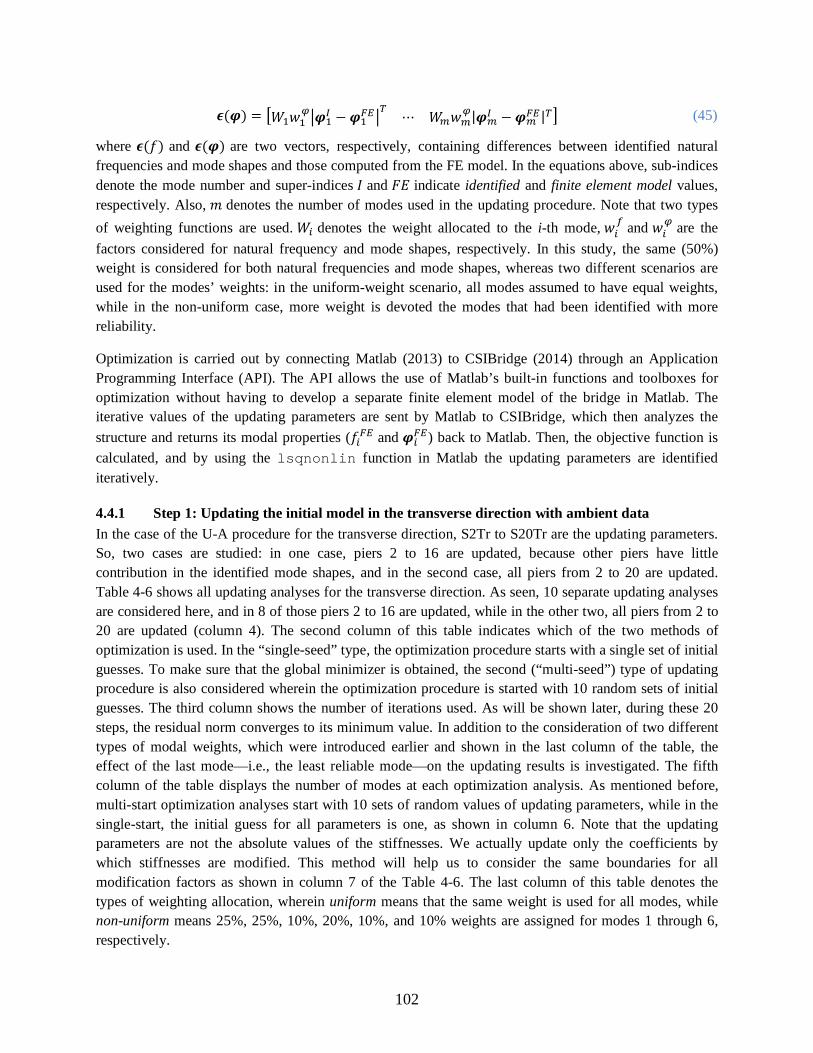
102

𝝐(𝝋) = �𝑊1𝑤1𝜑�𝝋1

𝐼 − 𝝋1𝐹𝐸�

𝑇⋯ 𝑊𝑚𝑤𝑚

𝜑|𝝋𝑚𝐼 − 𝝋𝑚

𝐹𝐸|𝑇� (45)

where 𝝐(𝑓) and 𝝐(𝝋) are two vectors, respectively, containing differences between identified natural frequencies and mode shapes and those computed from the FE model. In the equations above, sub-indices denote the mode number and super-indices 𝐼 and 𝐹𝐸 indicate identified and finite element model values, respectively. Also, 𝑚 denotes the number of modes used in the updating procedure. Note that two types of weighting functions are used. 𝑊𝑖 denotes the weight allocated to the i-th mode, 𝑤𝑖

𝑓 and 𝑤𝑖𝜑 are the

factors considered for natural frequency and mode shapes, respectively. In this study, the same (50%) weight is considered for both natural frequencies and mode shapes, whereas two different scenarios are used for the modes’ weights: in the uniform-weight scenario, all modes assumed to have equal weights, while in the non-uniform case, more weight is devoted the modes that had been identified with more reliability.

Optimization is carried out by connecting Matlab (2013) to CSIBridge (2014) through an Application Programming Interface (API). The API allows the use of Matlab’s built-in functions and toolboxes for optimization without having to develop a separate finite element model of the bridge in Matlab. The iterative values of the updating parameters are sent by Matlab to CSIBridge, which then analyzes the structure and returns its modal properties (𝑓𝑖𝐹𝐸 and 𝝋𝑖

𝐹𝐸) back to Matlab. Then, the objective function is calculated, and by using the lsqnonlin function in Matlab the updating parameters are identified iteratively.

4.4.1 Step 1: Updating the initial model in the transverse direction with ambient data In the case of the U-A procedure for the transverse direction, S2Tr to S20Tr are the updating parameters. So, two cases are studied: in one case, piers 2 to 16 are updated, because other piers have little contribution in the identified mode shapes, and in the second case, all piers from 2 to 20 are updated. Table 4-6 shows all updating analyses for the transverse direction. As seen, 10 separate updating analyses are considered here, and in 8 of those piers 2 to 16 are updated, while in the other two, all piers from 2 to 20 are updated (column 4). The second column of this table indicates which of the two methods of optimization is used. In the “single-seed” type, the optimization procedure starts with a single set of initial guesses. To make sure that the global minimizer is obtained, the second (“multi-seed”) type of updating procedure is also considered wherein the optimization procedure is started with 10 random sets of initial guesses. The third column shows the number of iterations used. As will be shown later, during these 20 steps, the residual norm converges to its minimum value. In addition to the consideration of two different types of modal weights, which were introduced earlier and shown in the last column of the table, the effect of the last mode—i.e., the least reliable mode—on the updating results is investigated. The fifth column of the table displays the number of modes at each optimization analysis. As mentioned before, multi-start optimization analyses start with 10 sets of random values of updating parameters, while in the single-start, the initial guess for all parameters is one, as shown in column 6. Note that the updating parameters are not the absolute values of the stiffnesses. We actually update only the coefficients by which stiffnesses are modified. This method will help us to consider the same boundaries for all modification factors as shown in column 7 of the Table 4-6. The last column of this table denotes the types of weighting allocation, wherein uniform means that the same weight is used for all modes, while non-uniform means 25%, 25%, 10%, 20%, 10%, and 10% weights are assigned for modes 1 through 6, respectively.

103

Table 4-6: Summary of updating analyses in the transverse direction.

No Single/Multi Seed Iteration Piers Modes Initial Guess Boundary Modal Weights

1 Single 20 2~16 1:6 Unit [0.1,10] Non uniform

2 Single 20 2~16 1:6 Unit [0.1,10] Uniform





7 Multi 20 2~16 1:6 Random [0.1,10] Non uniform

8 Multi 20 2~16 1:6 Random [0.1,10] Uniform

9 Multi 20 2~16 1:5 Random [0.1,10] Non uniform

10 Multi 20 2~16 1:5 Random [0.1,10] Uniform

Figure 4-5: Screenshot from the model updating procedure: MATLAB (left) and CSIBridge (right) are connected by an API for the updating procedures.

Figure 4-6 displays the modification factors obtained from 10 updating procedures for piers 2 to 16 (the results for the other 4 piers obtained from updating processes No. 3 and 4 are not shown). As this figure shows, the initial stiffnesses are approximately good, because modification factors are around 1.0 for most of the piers. Nevertheless, for most piers, especially those around the main span, the initial stiffnesses are smaller than the updated values. Another important point is that the modification factors for pier 2 and 16 are, respectively, very small and large (they are close to the boundaries considered for the optimization), which indicates insensitivity of the objective function (therefore, to the modal

104

properties used in its construction) with respect to these parameters. Finally, this figure shows that the results of the updating procedures using all these 10 analyses are all close to each other.

Figure 4-6: Modification factors obtained through the updating procedure.

• To see how well the updated models are matching the identified values, the MAC indices between the mode shapes of the updated FE models and real values are shown in

Table 4-7. In this table, the natural frequencies of the updated models are also shown, which can be compared with the identified values (1.00, 1.16, 1.33, 1.48, 1.60, 1.74). These results show that:

• Consideration of all piers during the updating procedure (i.e., No #3 and #4) does not improve the results.

• Allocation of higher weights to the more reliable modes (No #1) improves the updating results relative to the uniform weighting scheme (No #2) when all of the modes are included.

• The first five modes are almost identical to their identified counterparts in all analyses, while the sixth mode does not precisely follow the real-life data, which was expected (see, §3.4)

2 3 4 5 6 7 8 9 10 11 12 13 14 15 160

1

2

3

4

5

6

7

8

9

10

11

12

Pier No.

Mod

ifica

tion

Fact

or

No 01 No 02 No 03 No 04 No 05 No 06 No 07 No 08 No 09 No 10

105

• Multi-start optimization does not produce better results, so the current spring stiffnesses are the best initial guesses.

Table 4-7: Verification of the updated FE model in the transverse direction.

MAC Frequency (Hz) 1 2 3 4 5 6 1 2 3 4 5 6

No #1 0.97 0.95 0.88 0.88 0.87 0.77 1.00 1.16 1.33 1.48 1.60 1.75 No #2 0.95 0.94 0.92 0.87 0.84 0.82 1.00 1.16 1.33 1.48 1.61 1.75 No #3 0.97 0.95 0.89 0.89 0.88 0.74 1.00 1.16 1.33 1.48 1.61 1.76 No #4 0.95 0.94 0.92 0.87 0.85 0.81 1.00 1.16 1.33 1.48 1.61 1.75 No #5 0.97 0.96 0.88 0.90 0.90 0.02 1.00 1.16 1.33 1.48 1.60 1.60 No #6 0.97 0.95 0.93 0.89 0.90 0.05 1.00 1.16 1.33 1.48 1.60 1.73 N0 #7 0.97 0.95 0.88 0.88 0.87 0.64 1.00 1.16 1.33 1.48 1.60 1.75 No #8 0.95 0.94 0.92 0.87 0.84 0.71 1.00 1.16 1.33 1.48 1.60 1.75 No #9 0.96 0.96 0.88 0.91 0.88 0.02 1.00 1.16 1.33 1.48 1.60 1.61 No #10 0.97 0.95 0.93 0.89 0.90 0.03 1.00 1.16 1.33 1.48 1.60 1.69

4.4.2 Step 2: Updating the initial model in the longitudinal direction with ambient data As the soil-pile-foundation systems at all piers are almost symmetric, it is reasonable to expect similar stiffnesses along the longitudinal and transverse directions. Table 4-8 displays the MAC indices between the first longitudinal and vertical modes of the FE model, which is updated with the same factors obtained from transverse updating and their counterparts identified from real life data. As seen, mode shapes in both directions are not improved, because they were well matched to data. The initial FE model had MAC indices of 0.96 and 0.93 for longitudinal and vertical directions, respectively. A comparison of the natural frequencies of the updated models (Table 4-8) and the initial model reveals some improvement for the vertical direction; however, more updating is needed in these directions.

Table 4-8: Verification of the modified FE model in the longitudinal and vertical directions.

Longitudinal Vertical Frequency (Hz) MAC Frequency (Hz) MAC

No #1 1.24 0.92 1.65 0.91 No #2 1.23 0.92 1.65 0.91 No #3 1.23 0.95 1.65 0.91 No #4 1.20 0.93 1.65 0.91 No #5 1.19 0.90 1.66 0.91 No #6 1.23 0.91 1.65 0.91 No #7 1.24 0.92 1.65 0.91 No #8 1.23 0.92 1.65 0.91 No #9 1.19 0.90 1.65 0.91 No #10 1.22 0.91 1.65 0.91

106

As we do not have reliable mode shapes and natural frequencies of the higher modes for the longitudinal and vertical directions, we have to select as few updating parameters as possible to update the model in these directions. Sensitivity analyses showed that the sway stiffnesses in longitudinal direction at piers 3 to 13 have the highest contribution to the first longitudinal and vertical modes. Also, as both modes are identified with a high reliability, 50% weight is considered for both of them, and the equal weights are used for both natural frequencies and mode shapes. The previous results showed that these initial stiffnesses are very close to the actual values. As such, a single (instead of a multi-start) optimization analysis should be adequate. Figure 4-7 displays the variation of the residual norm during the optimization process, which rapidly converges to a very small constant value. After performing the optimization, natural frequencies of the first longitudinal and vertical modes are 1.40 and 1.76Hz, respectively, which are almost identical to the identified values (1.40 and 1.78Hz). The MAC indices are 0.99 for the longitudinal mode and 0.89 for the vertical mode. Note that for the vertical mode, only a few sensors are contributing to MAC indices, so a very small error will produce a significant MAC reduction.

Figure 4-7: Variation of norm of residual vector during

optimization process. Figure 4-8: Modification factors obtain after updating

process.

Although the updated longitudinal and vertical (especially longitudinal) modal properties of the system are perfectly matched to the identified values, the updated stiffness factors are not necessarily reasonable. Figure 4-8 shows that in order to match the modal properties, stiffnesses of some of piers must be multiplied by a very large factor, while some others must be multiplied by a very small value. This observed pattern is unreliable, because we expect to see the same variation as that observed in Figure 4-6. To see what exactly happened, the longitudinal mode shapes of the initial FE model (Case 1), model updated with the transverse stiffness (Case 2), and newly updated model (Case 3) are shown in Figure 4-9 along with the identified mode shape. As this figure clearly shows, optimization results of the transverse direction do not improve the quality of the longitudinal mode shape. As seen, by updating the pier 3 and 13’s stiffnesses along the longitudinal direction, the analytical mode shape is matched to the identified one, but this yields unrealistic modification factors as mentioned earlier.

The identified mode shape indicates that both ends of the bridge have very small deformations at the first longitudinal mode, which means that the abutment springs are almost fixed under ambient excitations, while large deformations are observed in the FE models using the current springs. For this reason, we

0 5 10 15 20 25

0.007

Iteration No.

Nor

m o

f Res

idua

l

0 2 4 6 8 100

2

4

6

8

10

Pier No.

Mod

ifica

tion

Fact

or

107

repeated an updating analysis on Case 3 in which left and right abutments’ springs were assumed as updating parameters, and we tried to minimize the objective function constructed using the first longitudinal mode’s properties. The updating procedure yielded large values for the abutment springs (i.e., ~8.9 and ~5.4 times of the current values of the left and right abutment stiffnesses, respectively) for which the natural frequency would be 1.41Hz, which is very close to the identified value. The mode shape of this new model is also shown in Figure 4-9 as Case 4. As seen, neglecting unusual deformations at a few points, the mode shape is close to the identified and the MAC value for this case is 0.99. These results shows that the optimization process should be repeated in the longitudinal direction with piers 3 to 13 as updating parameters, while abutments are almost fixed.

Figure 4-9: First longitudinal mode shape.

Figure 4-10 displays the new modification factors of the pier stiffnesses along the longitudinal direction after assuming almost fixed abutments. As seen, the estimated values vary around 1.0, which is realistic. The first longitudinal and vertical natural frequencies of this new updated model are 1.40 and 1.72, respectively. These values are almost identical for the longitudinal direction, and have only a small error for the vertical direction. Note that the natural frequency and the mode shape of the vertical direction may be sensitive to other factors like the mass of the superstructure. MAC indices for these two modes of the final updated model with respect to the identified mode shapes are 1.00 and 0.96, for the longitudinal and vertical directions, respectively. That is now a perfect match in longitudinal direction. Figure 4-11 shows the newly updated first longitudinal mode shape along with the identified and initial mode shapes. This figure clearly displays that the updating procedure has successfully converged to the identified mode shape.

S1 S2 S3 S4 S5 S6 S7 S8 S9 S10 S11 S12 S13 S14 S15 S16 S17 S18 S19 S20 S21

1

Pier No.

Identified

Case 1

Case 2

Case 3

Case 4

108

Figure 4-10: Modification factors obtained after the updating procedure.

Figure 4-11: Identified, initial, and updated first longitudinal mode shapes.

4.4.3 Step 3: Updating the ambient model in the transverse direction with weak earthquake data As it was shown in the previous chapter, modal properties identified from earthquake data (both weak and severe) are different from those identified from the ambient test data. Therefore, the FE model updated through the first and second steps above does not represent the behavior of the bridge during earthquakes. At this section, we attempt to update the FE model (along the transverse direction first) so that it can capture the real-life behavior of the bridge during weak earthquakes. As a representative sample for weak earthquakes, we use the modal properties identified form the Willow Creek earthquake (2008) to update the bridge in the transverse direction. Table 4-9 shows the initial differences between the FE model updated using ambient data and the identification results from the earthquake data.

3 4 5 6 7 8 9 10 11 12 130

0.4

0.8

1.2

1.6

2

Pier No.

Mod

ifica

tion

Fact

or

S1 S2 S3 S4 S5 S6 S7 S8 S9 S10 S11 S12 S13 S14 S15 S16 S17 S18 S19 S20 S21

1

Pier No.

Identified

Case 1

Case 5

109

Table 4-9: Comparison of modal properties identified from Willow Creek earthquake (2008) and FE model updated by ambient data.

Mode No. Frequency (Hz) MAC (%) FE Model Identified Error (%) 1 1.00 0.91 9.89 0.98 2 1.16 1.10 5.45 0.64 3 1.33 1.14 16.67 0.92 4 1.48 1.30 13.85 0.65 5 1.60 1.47 8.84 0.74 6 1.75 1.55 12.90 0.23

Unlike the case for ambient vibrations, the columns likely exhibit cracked behavior, and thus the cracking effect is added in as one of the updating parameters (C2Tr to C20Tr) here. Moreover, due to soil nonlinearity, the soil-pile springs’ coefficients may change. So, by assuming an equivalent linear model, we should consider a reduction factor for each previously updated stiffness coefficient (N2Tr to N20Tr). Furthermore, the identified mode shapes suggest that the abutments displayed movement in some of the modes. Hence, abutment stiffnesses are also included among the updating parameters (LATr and RATr). Accordingly, we have 19+19+2=40 updating parameters. This is a very large number and thus we attempt to reduce them through reasonable assumptions prior to updating. The first assumption is to consider the same cracking factor for all piers. The second assumption is to apply the same reduction factor for all piers to account for soil nonlinearity. We reserve the option to consider a separate factor for each pier later, if the updating procedure does not yield acceptable results. One these two sets of assumptions are made, the number of updating parameters will reduce to 4 parameters.

Again, we employ the previously mentioned multi-start optimization method in Matlab. To reduce the number of analyses, we consider equal weights for all modes. MAC indices for the first to sixth modes are 0.97, 0.61, 0.93, 0.79, 0.59, and 0.39, respectively. By comparing these values with those reported in Table 4-9, no improvement is seen for the mode shapes (note that the MAC indices are calculated only at the instrument locations). However, the natural frequencies are 0.89, 1.05, 1.20, 1.34, 144, and 1.55 Hz, which are now closer to the identified values. These updated modal properties are obtained provided that moments of inertia of the columns are reduced by a factor of 0.56 (i.e., C2Tr to C20Tr = 0.56), all soil-pile spring stiffnesses are reduced by a factor of 0.80 (i.e., N2Tr to N20Tr = 0.80), and the abutments have almost their current transverse stiffnesses (i.e., LATr =1.00 and RATr = 0.92).

As seen, the modal properties, especially the mode shapes, are well matched to their counterparts identified from recorded data. Therefore, considering the same nonlinearity factor for all piers is no longer a reasonable assumption, and we have to repeat the optimization process by considering additional updating parameters—namely, N2Tr to N20Tr. On the other hand, the abutment stiffnesses can be considered constant. Accordingly, we have 19+1 = 20 updating parameters.

In what follows, three scenarios are considered—each with a different lower-bound for the nonlinearity coefficients, and with lower- and upper-bounds for the CT factor of 0.5 and 1, respectively. Table 4-10 displays the modal properties of the updated FE model obtained for the said three scenarios and their

110

errors with respect to the identified values. The lower-bound for the nonlinearity reduction factors are 0.1, 0.5, and 0.7 for the scenarios I, II, and III, respectively; while the upper bound is always 1.0

Table 4-10: Modal properties identified from the 2008 Willow Creek earthquake, and those computed from the FE model updated using ambient data.

Mode No. Scenario I Scenario II Scenario III

Frequency Error (%) MAC Frequency

Error (%) MAC Frequency Error (%) MAC

1 0.39 0.98 0.51 0.98 1.34 0.98 2 2.35 0.89 2.75 0.87 1.88 0.73 3 1.20 0.94 1.60 0.93 4.53 0.94 4 0.89 0.93 0.94 0.93 3.18 0.89 5 2.80 0.90 2.51 0.90 1.69 0.80 6 0.15 0.62 0.48 0.55 0.25 0.52

The CT factor for the scenarios I, II, and III are 0.89, 0.66, and 0.54, respectively. Figure 4-12 displays the nonlinearity factors for all piers after these updating processes. Several observations can be made:

• Piers 18 to 20 are unchanged (except for pier No. 20 for the updating scenario I), because we do not have significant information about the mode shapes at these points.

• Except for piers 3, 12, 14, 15, 16, and 17, the piers’ stiffness coefficients are the same for all three scenarios. So, their average values can be selected.

• Also considering the observation made above about the pier stiffnesses, Figure 4-12 suggests that imposing a higher lower-bound renders the third scenario’s results different from the other two. Moreover, Table 4-10 indicates that results from scenario III have lower accuracy. Therefore, this scenario’s results will be discarded. As such, the differences between the model and the identified modal data are now only related to piers 3, 14, 15, and 16.

• As the stiffnesses of piers 3, 14, 15, and 16 are equal to the considered lower-bound for scenario II, they are likely to be unreliable. So, we consider the first scenario’s results as the true ones. Interestingly, those piers that display the highest nonlinearity (i.e., smallest nonlinearity factor) are also the piers that have the largest embedment into the soil.

2 3 4 5 6 7 8 9 10 11 12 13 14 15 16 17 18 19 20

0

0.2

0.4

0.6

0.8

1

Pier No.

Non

linea

rity

Fact

or

I II III

111

Figure 4-12: N2Tr through N20Tr factors for three updating scenarios.

4.4.4 Step 4: Updating the ambient model in the longitudinal direction with weak earthquake data To update the FE model in the longitudinal direction, we use the first natural frequency and mode shape identified from Ferndale earthquake (2007) as representative of the weak earthquakes (we do not use the modal properties identified from the 2008 Willow Creek earthquake, because those results appeared doubtful along the longitudinal direction). In the longitudinal direction, the number of sensors is even smaller than the transverse. However, it is expected to get almost accurate results if we use cracking and nonlinearity factors obtained in the transverse direction for the longitudinal direction as well. Interestingly, by using these factors, natural frequency of the first longitudinal mode of the FE model changes from 1.40 Hz to 1.21 Hz, which is exactly the same value identified from real-life data! Also, MAC changes from 0.96 to 0.99! The first vertical natural frequency of the FE model, which was initially 1.72 Hz, decreases to 1.63 Hz. The identified value was 1.68 Hz in the Ferndale earthquake 2007. We do not try to further update the model in the vertical direction, because we do not have adequate data to search beyond the first mode in the direction.

4.4.5 Step 5: Updating the weak earthquake model in transverse direction with strong earthquake data In this step, we attempt to update the already updated FE model (last two steps) in the transverse direction using modal properties identified from the Ferndale earthquake 2010, which is a relatively severe earthquake. For this earthquake, the mode shapes are not identified at all of the previously used channels (there was no data from channels #22-24). Also, the data recorded at channel #18 looks unusual as shown in Figure 4-13. As seen, the recorded motion at this channel features several spikes. The same channel malfunctioned during our ambient tests in 2013 as well, and was producing noise as shown in Figure 4-14. As such, we have the transverse mode shapes at a very limited number of points for the present case, which inherently reduces the reliability of the updating procedure.

Figure 4-13: Recorded signals by channels #15 and #18 during the 2010 Ferndale earthquake.

0 10 20 30 40 50 60 70 80 90-0.4

-0.2

0

0.2

0.4

Time (sec.)

Acc

eler

atio

n (g

)

Ch 15Ch 18

112

Figure 4-14: Recorded signals by channels #15 and #18 during the 2013 ambient tests.

Because of the aforementioned sensor limitations, we exclude the abutment stiffnesses from the updating procedure. Also, we consider the same cracking factor for all piers, and use the factor obtained from weak earthquakes as the upper bound and 0.5 as the lower bound. A preliminary updating procedure showed that it is not possible to attain good results by employing the same nonlinearity factor for all piers (details not presented for brevity). Also, we found that the stiffnesses of piers No. 16 to 20 do not play important roles on the modal properties, because we do not have adequate information at the right-end of the bridge for this earthquake. Therefore, we excluded them from the updating procedure. Moreover, we considered 1.0 as the upper bound for all nonlinearity factors (N2Tr to N15Tr), because stiffnesses must be lower for the present case than those for the weak earthquakes.

The updating procedure showed that the cracking factor, which was 0.89 for the weak earthquakes, should be considered as 0.5 for this severe earthquake. Figure 4-15 displays the modification factors obtained from the updating process. As seen, the equivalent stiffnesses of the piers are reduced by factors less than 0.8 during the severe portion of the Ferndale earthquake, 2010. Finally, Table 4-11 displays the modal properties of the updated model, the initial values—i.e., those obtained from the FE model updated using the weak earthquake data—and the identified values from the 2010 Ferndale earthquake data. As seen, the updated model has modal properties—especially natural frequencies—that are very close to the values identified from real-life data. It is important to note here that we assumed 50% weight for the first mode and 10% for all other modes, because of higher identification uncertainties for those higher modes due to sparse instrumentation.

Table 4-11: Comparison of modal properties of initial FE model (updated using weak earthquake data) and updated FE model with values identified form Ferndale earthquake (2010).

Mode No. Identified Initial FE Updated FE Frequency

(Hz) Frequency

(Hz) MAC Frequency (Hz) MAC

1 0.68 0.91 0.92 0.65 0.91 2 0.77 1.07 0.89 0.78 0.92

10 12 13 14 15 16 17 18 19 20 21 22 23 0 1 2 3 4 5 6 7 8 9 10

0

x 10-19

Time (hr)

Ch 15Ch 18

113

3 0.86 1.15 0.73 0.84 0.75 4 0.98 1.31 0.80 0.99 0.80 5 1.02 1.43 0.39 1.05 0.50 6 1.13 1.55 0.10 1.12 0.69

Figure 4-15: Modification factors obtained from severe part of the Ferndale earthquake, 2010.

4.4.6 Step 6: Updating the weak earthquake model in longitudinal direction with strong earthquake data Similar to the weak earthquakes, we expected to attain accurate results for the longitudinal direction if we use the cracking and nonlinearity factors obtained in the transverse direction, as well. Again, and quite interestingly, by using the factors obtained for the transverse direction, the natural frequency of the first longitudinal mode of the initial FE model changes from 1.21 Hz to 0.66 Hz, which is very close to the value identified from real-life data (it was 0.67)! However, the MAC index changes from 0.97 to 0.95, which means mode shape is not very accurate. This was possibly due to the fact that we did not modify the stiffnesses of piers No. 16 to 20, even though they may have significant effects on the longitudinal mode shape. To improve the updating results, we then repeated the updating procedure for the longitudinal direction. However, we condensed the updating parameters because of the limited number data channels. Specifically, we assumed a constant cracking factor 0.5 for all columns and identical stiffness factors for both abutments; and we also grouped the nonlinearity factors for piers based on their similarities observed up to this point (specifically, we assumed identical updating factor for piers 2 and 3, piers 4 to 13, and piers 14 20). Based on these assumptions, we only have 4 factors to be updated using the longitudinal modal data identified from (severe portion of) the 2010 Ferndale earthquake.

By updating the model, natural frequency changed from 1.21 to 0.67 (i.e., the identified value from 2010 Ferndale exactly!), and also the MAC index became 0.98. The updated model shows that the abutment stiffnesses in the longitudinal direction must be reduced by a factor of 0.67 with respect to the weak

2 3 4 5 6 7 8 9 10 11 12 13 14 150

0.2

0.4

0.6

0.8

1

Pier No.

Mod

ifica

tion

Fact

or

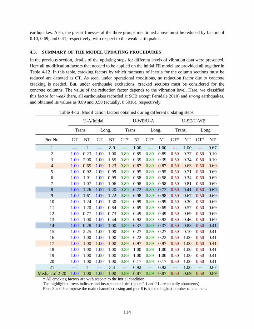
114

earthquakes. Also, the pier stiffnesses of the three groups mentioned above must be reduced by factors of 0.10, 0.69, and 0.41, respectively, with respect to the weak earthquakes.

4.5. SUMMARY OF THE MODEL UPDATING PROCEDURES

In the previous section, details of the updating steps for different levels of vibration data were presented. Here all modification factors that needed to be applied on the initial FE model are provided all together in Table 4-12. In this table, cracking factors by which moments of inertia for the column sections must be reduced are denoted as CT. As seen, under operational conditions, no reduction factor due to concrete cracking is needed. But, under earthquake excitations, cracked sections must be considered for the concrete columns. The value of the reduction factor depends to the vibration level. Here, we classified this factor for weak (here, all earthquakes recorded at SCB except Ferndale 2010) and strong earthquakes, and obtained its values as 0.89 and 0.50 (actually, 0.5016), respectively.

Table 4-12: Modification factors obtained during different updating steps.

U-A/Initial U-WE/U-A U-SE/U-WE

Trans. Long. Trans. Long. Trans. Long.

Pier No. CT NT CT NT CT* NT CT* NT CT* NT CT* NT

1 --- 1 --- 8.9 --- 1.00 --- 1.00 --- 1.00 --- 0.67 2 1.00 0.23 1.00 1.00 0.89 0.89 0.89 0.89 0.50 0.77 0.50 0.10 3 1.00 2.00 1.00 1.55 0.89 0.39 0.89 0.39 0.50 0.34 0.50 0.10 4 1.00 0.65 1.00 1.23 0.89 0.87 0.89 0.87 0.50 0.63 0.50 0.69 5 1.00 0.92 1.00 0.99 0.89 0.95 0.89 0.95 0.50 0.71 0.50 0.69 6 1.00 1.01 1.00 0.99 0.89 0.58 0.89 0.58 0.50 0.34 0.50 0.69 7 1.00 1.07 1.00 1.06 0.89 0.98 0.89 0.98 0.50 0.81 0.50 0.69 8 1.00 1.26 1.00 1.20 0.89 0.72 0.89 0.72 0.50 0.41 0.50 0.69 9 1.00 1.61 1.00 1.22 0.89 0.98 0.89 0.98 0.50 0.67 0.50 0.69

10 1.00 1.24 1.00 1.30 0.89 0.99 0.89 0.99 0.50 0.30 0.50 0.69 11 1.00 1.20 1.00 0.84 0.89 0.69 0.89 0.69 0.50 0.57 0.50 0.69 12 1.00 0.77 1.00 0.73 0.89 0.49 0.89 0.49 0.50 0.69 0.50 0.69 13 1.00 1.00 1.00 0.44 0.89 0.92 0.89 0.92 0.50 0.46 0.50 0.69 14 1.00 0.28 1.00 1.00 0.89 0.37 0.89 0.37 0.50 0.85 0.50 0.41 15 1.00 2.25 1.00 1.00 0.89 0.27 0.89 0.27 0.50 0.10 0.50 0.41 16 1.00 1.00 1.00 1.00 0.89 0.22 0.89 0.22 0.50 1.00 0.50 0.41 17 1.00 1.00 1.00 1.00 0.89 0.97 0.89 0.97 0.50 1.00 0.50 0.41 18 1.00 1.00 1.00 1.00 0.89 1.00 0.89 1.00 0.50 1.00 0.50 0.41 19 1.00 1.00 1.00 1.00 0.89 1.00 0.89 1.00 0.50 1.00 0.50 0.41 20 1.00 1.00 1.00 1.00 0.89 0.17 0.89 0.17 0.50 1.00 0.50 0.41 21 --- 1 --- 5.4 --- 0.92 --- 0.92 --- 1.00 --- 0.67

Median of 2-20 1.00 1.00 1.00 1.00 0.89 0.87 0.89 0.87 0.50 0.69 0.50 0.69 * All cracking factors are with respect to the initial condition. The highlighted rows indicate and instrumented pier (“piers” 1 and 21 are actually abutments). Piers 8 and 9 comprise the main channel crossing and pier 8 is has the highest number of channels.

115

Another uncertain and important factor that was studied extensively here was that for the soil-pile stiffnesses, which are shown in the NT columns. As seen in Table 4-12, the initial value for the abutment stiffnesses (i.e., “piers” 1 and 21) in the longitudinal direction was much lower than the value obtained from ambient test data. This large drop in the longitudinal abutment stiffness from initial to ambient can be attributed the gap between the deck and the abutment backwalls, which was not taken into account in the initial model. Once the updates were made to the abutment stiffnesses using ambient data, the behavior for weak earthquakes remained the nearly the same as that for operational conditions (see, Figure 4-16). For higher level of vibrations, the abutment stiffnesses did not change significantly, except for the severe portion of Ferndale 2010, for which the longitudinal stiffnesses reduced significantly (also shown in Figure 4-16)—indicating potential nonlinearity. However, sparseness of the SCB’s sensor array around the abutments prevents us from providing a definitive statement on the abutment behavior during earthquakes.

Figure 4-16: Modification factors for abutment stiffness with respect to stiffnesses identified from ambient data.

For the other piers (i.e., pile groups), the stiffnesses of the initial model were very close to values identified from operational conditions (see Table 4-12 and Figure 4-17). However, stiffnesses of some of the piers—especially those that have larger embedment—were drastically reduced during even the weak earthquakes (Figure 4-18). The reduction in the pier stiffnesses increased with increasing levels of input excitations (as it can be seen clearly for the severe portion of the 2010 Ferndale earthquake).

116

Figure 4-17: Modification factors for the initial model’s pile-group stiffnesses identified from ambient data.

Figure 4-18: Modification factors for the pile-group stiffnesses with respect to values identified from ambient data.

117

4.6. RESPONSE PREDICTION STUDIES AND UPDATING THE INPUT MOTIONS

4.6.1 Prediction of recorded time-history responses using the updated FE models As mentioned previously, input motions are not directly available, because the system, in general, would experience multiple support excitations, while data is only recorded at one pile-tip (channels #31, #33, and #33). Moreover, the signals recorded at the pile-tip cannot be assumed as input motions because of soil-structure interaction effects. Nevertheless, we computed the response of the bridge system using the updated FE models and by applying only the pile-tip motions (i.e., signals recorded at channels #31, #32, an #33 that were corrected as described in §2.3.2) simultaneously at all of the supports. These responses are compared to real-life records at various instrumentation points below for different events.

Figure 4-19: Comparison of recorded and calculated response signals for the 2007 Ferndale earthquake.

Figure 4-19 and Figure 4-20 display the time-history of the response of the U-WE finite element model at two directions for the 2007 Ferndale, and the 2008 Willow Creek earthquakes, respectively, along with the real-life/recorded signals. To produce these graphs, the input motion along the longitudinal direction was multiplied by a factor of 1.36, and a Rayleigh model was to be considered for the damping. The damping ratios were set at two frequencies (0.7 Hz, and 5 Hz) such that the peak responses are matched. As seen from the figures, although the same FE model was used for two different earthquakes, the recorded and predicted response signals agree well with each other for both earthquakes, for both directions. The only inconsistency is observed during a brief initial time period of the 2008 Willow Creek

20 25 30 35 40 45 50 55-0.3

-0.15

0

0.15

0.3

0.45

Time (sec.)

Dis

plac

emen

t (cm

)

Recorded Ch #11 FE Model

20 25 30 35 40 45 50 55-0.4

-0.2

0

0.2

0.4

Time (sec.)

Dis

plac

emen

t (cm

)


118

earthquake in the longitudinal direction. However, the frequency content seems identical and thus the differences must be related to the input motions.

Figure 4-20: Comparison of recorded and calculated response signals for the 2008 Willow Creek earthquake.

Remarks: The aforementioned ad hoc increase that needed to be applied to the longitudinal input motion amplitude can be attributed to several factors:

• Kinematic interaction effects imply that pile input motions are generally reduced versions of the free field motions (see, for example, Anoyatis et al., 2013). Since we are applying the input motions at the remote ends of the updated springs, the input motions, in general, are expected to be amplified versions of the recorded motions.

• The amplification factor had to be applied only along the longitudinal direction. This implies two possibilities that are not mutually exclusive: (i) the motions recorded at the pile-tip have a bias (for example, due to a local anomaly that prevents accurate measurements); (ii) kinematic interaction plays a more prominent role along the longitudinal direction. The latter possibility has to be viewed with the understanding that the bridge system acts almost monolithically along the longitudinal direction, whereas mode shapes along the transverse direction suggest several segments acting together. This means that any error in the predicted input motion along the longitudinal direction will have a proportionally larger impact on the observed/predicted overall response in the superstructure. Finally, the longitudinal response amplitudes of the bridge system are typically less than the transverse ones, and thus the effect of the fairly large factor of 1.36 on the overall bridge system response is not necessarily large.

15 20 25 30 35 40 45 50 55 60-0.35

0

0.35

Time (sec.)

Dis

plac

emen

t (cm

)


15 20 25 30 35 40 45 50 55 60-0.7

-0.35

0

0.35

0.7

Time (sec.)

Dis

plac

emen

t (cm

)


119

• The rocking stiffnesses of pile groups are much smaller along the transverse direction than they are along the longitudinal direction. Moreover, we have lumped the pile stiffnesses into matrix representations at the pile-caps. We are only applying translational input motions to the pile caps through the lumped springs, but in reality, input motions distributed along the piles can cause the pile groups to rock. This effect is completely removed due to lumping, and a portion of the amplification factor (of 1.36) may be alleviating this erasure.

Given these considerations, it is fair to state that neither of the possibilities above can be ruled out. More definitive findings may be attained if there were more pile-tip measurements (within a given group, and also at multiple pile groups). Detailed kinematic interaction studies using continuum finite element models of the pile groups and their surrounding soil media can also yield useful results.

Figure 4-21: Comparison of recorded and calculated response signals for the 2008 Trinidad earthquake.

The time-history comparisons presented above are for earthquakes that have been used for model updating. That is, we used the transverse modal properties identified from the 2008 Willow Creek earthquake, and longitudinal modal properties identified from the 2007 Ferndale 2007 for updating the U-WE FE model as described earlier. As such, the good match between the observed and the predicted responses for these two events should not be surprising. Indeed, it is more interesting (and fair) to compare responses predicted using the updated FE model with signals recorded in a different earthquake (i.e., an event that was not using for FE updating). Figure 4-21 presents such a comparison for the 2008 Trinidad earthquake 2008 (again, the longitudinal pile-tip motion had been multiplied by 1.36 for this

15 20 25 30 35 40 45 50 55 60-0.25

0

0.25

Time (sec.)

Dis

plac

emen

t (cm

)


15 20 25 30 35 40 45 50 55 60-0.3

-0.15

0

0.15

0.3

Time (sec.)

Dis

plac

emen

t (cm

)


120

simulation). As seen, the compatibility is satisfactory for both directions, especially in the transverse direction, which validates the updated U-WE FE model and the amplification factor of 1.36 for the longitudinal direction.

To verify the FE model updated for severe earthquakes (i.e., the U-SE model), we present comparisons between signals recorded during the 2010 Ferndale earthquake, and those predicted by the U-SE FE model. For this earthquake, we used the same Rayleigh damping model, but increased the damping ratios from 2% to 5% to account for higher level of nonlinearities. As Figure 4-22 shows, the transverse and longitudinal responses are compatible with their recorded counterparts, but only during the time period that we used for the identification purposes—i.e., from 28 to 56 seconds. The match is especially good between 38 and 50 seconds when the system exhibited it lowest natural frequency, as already discussed in §3.4.2 (see, also Figure 3-31 and Figure 3-32). In the other words, system’s modal properties are changing during the event, and thus an equivalent linear model cannot predict the system response at all times with the same accuracy.

Figure 4-22: Comparison of recorded and calculated response signals for the 2010 Ferndale earthquake.

20 30 40 50 60 70 80 90-20

-10

0

10

20

Time (sec.)

Dis

plac

emen

t (cm

)


20 30 40 50 60 70 80 90-10

0

10

Time (sec.)

Dis

plac

emen

t (cm

)


121

In order to produce a more general predictive model, we opted to replace the updated equivalent linear soil springs with bilinear springs. For each bilinear spring, we assigned the stiffness used for the U-WE FE model as the initial stiffness, and the stiffness of the U-SE FE model as the secondary stiffness. Also, we used the maximum spring deformations of the U-WE FE model during the weak events used in its calibration as the yield deformations of the new bilinear soil springs. Subsequently, we analyzed the new FE model under the input motion of the 2010 Ferndale earthquake 2010. Figure 4-23 presents same graphs as Figure 4-22 but for the new FE model with bilinear soil springs. As seen, the compatibility is almost perfect for both directions. That is, the new FE model is able to reproduce the behavior of the Samoa Channel Bridge under any level of input excitations (that it had experienced thus far) with very good accuracy.

Figure 4-23: Comparison of recorded and calculated (using the new FE model with bilinear springs) response signals for the 2010 Ferndale earthquake.

To complete this section, a figure that is similar to Figure 3-31 is shown in Figure 4-24, which is produce by replacing the signal recorded at channel #6 by its counterpart that is predicted by the updated FE model with bilinear springs. As this figure shows, the natural frequency of the system, which is initially about 1.21 Hz (because the system has initial stiffness that identical to the U-WE model), suddenly drops to 0.79 Hz when the severe waves arrive. It then gradually decreases to the lowest level (0.68 Hz) during

20 30 40 50 60 70 80 90-20

-10

0

10

20

Time (sec.)

Dis

plac

emen

t (cm

)


20 30 40 50 60 70 80 90-10

0

10

Time (sec.)

Dis

plac

emen

t (cm

)


122

the time interval of 40 to 50 seconds. After this time window ends, the natural frequency of the actual system recovers but not to its initial value due to permanent stiffness degradation. However, as we did not incorporate stiffness degradation into our final FE model, the natural frequency eventually recovers to its initial value (i.e., 1.21 Hz). As we did not incorporate a time-varying cracking factor to this model either, we had to consider an average factor of 0.50 for the entire time of analysis. Hence, its initial frequency 0.86 Hz, as seen in seen in Figure 4-24. These additional modifications can be made to improve the overall fit even further, but will not be pursued here, as they will not significantly enhance the findings obtained thus far on the seismic behavior of the Samoa Channel Bridge.

Figure 4-24: Time-frequency representation of the response of the FE model during the 2010 Ferndale earthquake recorded at channel #6.

4.6.2 Postscript: Blind Predictions for the Ferndale earthquake of March 9, 2014 During the completion of this report, an earthquake occurred on March 09, 2014. This Ferndale earthquake had a 6.8ML and its epicenter was 81.3 km away from the Samoa Channel Bridge. Maximum acceleration recorded on the deck was approximately 0.069g; and this intensity is similar to the weak earthquakes recorded on the bridge before. Again, we used the pile-tip channels’ data (Ch. #31, #32, and #33) as input accelerations at all piers and predicted the response of the bridge using our final FE model with no modification. Figure 4-25 displays this comparison for the same channels used for the other earthquakes. It is important to note that, as we did with all previous earthquakes, we used the corrected versions of the input accelerations and we also used the same amplification factor (i.e., 1.36) for the longitudinal direction. As seen, the current model accurately reproduced the recorded response of the bridge for this earthquake (this is a complete blind prediction). This finding implies that predictions for

Time (Sec.)

Freq

uenc

y (H

z)

0 10 20 30 40 50 60 70 80 900.5

0.6

0.7

0.8

0.9

1

0.68 Hz

0.78 Hz

0.79 Hz

0.86 Hz

123

future earthquakes can be carried using the final FE model produced in this project with fairly good confidence.

Figure 4-25: Comparison of recorded and calculated response signals for the 2014 Ferndale earthquake

0 10 20 30 40 50 60 70 80 90 100-2.5

0

2.5

Time (sec.)

Dis

plac

emen

t (cm

)


0 10 20 30 40 50 60 70 80 90 100-4

0

4

Time (sec.)

Dis

plac

emen

t (cm

)


125

Chapter 5 SUMMARY OF FINDINGS AND RECOMMENDATIONS

In this project, results of a detailed investigation on the Samoa Channel Bridge were presented. The study began with an overview of the bridge characteristics, its CSMIP instrument array, and the seismic data recorded to date by that array (0). A detailed discussion of the various features of recorded data and preliminary signal processing studies were presented in Chapter 1. A novel output-only system identification method was introduced and applied in Chapter 1 to extract the bridge’s modal characteristics using data from recorded strong motion events as well as an ambient survey that was carried out in June 2013. The development of an initial finite element model using structural drawings and available geotechnical data, and the updating of this model to match the recorded responses were presented in Chapter 1.

Major findings of this study are:

• True Orientations of In-Pile Sensors (Chapter 2.3): The data recorded at various in-pile sensors at Pier 8 required corrections. In prior studies, CGS realized an alignment problem with the pile-tip sensor package (specifically, Channels #31 and #33) and offered a correction. While CGS provided this correction only for the 2010 Ferndale data, the present study confirms that it should be applied to all other earthquake data as well. Moreover, in the present study, and the true orientations of two other in-pile channels—namely, Channels #28, and #30, which are also at Pier 8—were computed using a cross-correlation analysis technique. The said technique exploited the presence soil-structure-interaction effects, and was validated using two on-deck channels for which the true orientations are well known. In future studies, all data from Channels #28, #30, #31, and #33 should be re-oriented as described in Chapter 2, prior to any analysis.

• Wave Passage Effects (Chapter 2.4): Seismic waves arrive the two abutments of the bridge at different times, depending on the direction of arrival of seismic waves. The time-lag values obtained for different earthquakes reached above 200 ms, and the computed values were generally consistent with the known/reported epicenters of those events. The effects of the observed time lags did not appear to be significant in the overall transverse responses of the bridge. However, pounding occurred during the 2010 Ferndale, and this was likely, in part, due to a delayed excitation of the different segments of the bridge.

• Validation of Site Soil Profile (Chapter 2.5): Cross-correlation techniques were also used to estimate the shear wave velocities using data from the nearby geotechnical array, and the computed values agreed fairly well with values obtained by Caltrans/CGS from borehole logging tests.

• Presence of Inertial Soil-Structure-Interaction (SSI) Effects (Chapter 1): Initial studies using basic peak-picking methods indicated significant presence of SSI effects for the Samoa Bridge during all earthquakes, as the recorded pile-cap and in-pile motions displayed prominent peaks at (flexible-base) structural frequencies15. Even the signals recorded at the free-field station—which is located 160 ft away from the north abutment (see, Figure 1-11)—contained prominent peaks at the first longitudinal flexible-base structure frequency.

15 These are actually combined soil-foundation-superstructure frequencies, which are often referred to as “flexible-base structure” frequencies.

126

• Application of a Novel Output-Only Modal Identification Method (Chapters 3.2 and 3.3): The strong presence of SSI meant that input-output modal identification methods are not applicable. Since strong motion events are non-stationary, conventional output-only modal identification methods could not be used either. As such, a novel output-only identification method that was recently devised by the PI’s team (Abazarsa et al, 2013ab; Ghahari et al., 2013abc) had to be used to identify the natural frequencies and mode shapes of the Samoa Bridge from earthquake data (§3.4.2)

• Ambient Vibration Survey (Chapter 3.4.1): The sparseness of CSMIP instruments on the superstructure prevented the determination of mode shapes with resolution that is adequate for finite element model updating. This necessitated an ambient vibration survey, which was carried out as part of this project in June 2013 and yielded mode shapes with a much better resolution. These results enabled accurate finite element model updating studies. It is also expedient to note that here both the ambient vibration survey and the earthquake data suggested a fairly monolithic response along the longitudinal direction. On the other hand, the bridge behaved as a more-or-less segmented structure along the transverse direction.

• Finite Element Model Updating Studies (Chapters 4.1-4.4): CSIBridge and Matlab were connected to each other through an Application Programming Interface and by employing a systematic optimization procedure, the initial finite element model was updated, in various stages, first to match modal properties identified from the ambient survey, then from several weak earthquakes together, and finally from the only strong earthquake to date, the 2010 Ferndale Earthquake. Model updating studies yielded stiffness factors for the columns, pile groups, and abutments, and key information about the foundation input motions. The stiffness factors were seen to be highly dependent on the amplitude/strength of shaking.

• Finite Element Model Updating Results on Column Stiffnesses (Chapter 4.5): Column stiffnesses were observed to be 1.0, 0.86, and 0.50 times the nominal (gross) values under operational (ambient) conditions, weak earthquakes, and the strong earthquake, respectively (Table 4-12).

• Finite Element Model Updating Results on Equivalent Abutment Stiffnesses (Chapter 4.5): Abutment stiffnesses did not play a large role in the responses recorded to date, because even for the strongest earthquake the amplitudes of motion at the abutments were low. Nonetheless, the nominal abutment stiffness values yielded good fits with modal properties identified from operational conditions as well as weak earthquakes. The factors reduced to 67% along the longitudinal direction for both abutments during the strong earthquake, while the transverse direction stiffness remained unchanged. These results are compactly presented in Table 4-12, and Figure 4-16.

• Finite Element Model Updating Results on Equivalent Pile Group Stiffnesses (Chapter 4.5): While there were some variations in stiffness factors from pier to pier, it is reasonable to assume that results for instrumented piers (4, 8, 9, 14, 17) are more reliable because their values control the observed responses more than the other piers. Moreover, the pile group stiffnesses obtained only at the piers of the main channel crossing—especially, pier 8, which is the most instrumented pier—play the most important role, because responses from other piers had much smaller amplitudes. Given this presumptive bias, we conclude that the nominal pile-soil interaction stiffnesses were more or less appropriate for ambient/operational conditions (actually, operational stiffness of the pier 8 pile group was ~20% higher than what

127

was used in the initial model). From operational conditions to weak earthquakes, the median value of the back-calculated pile-group stiffness factors was 87% for all piers; and from weak earthquakes to the strong earthquake—i.e., 2010 Ferndale, for which there was strong evidence of soil nonlinearity—the median factor was 69%. There were no discernable differences between the stiffness factors for the transverse and longitudinal directions. These results are compactly presented in Table 4-12, Figure 4-17, and Figure 4-18.

• Predictions of Time-History Data and Foundation Input Motions (Chapter 4.6): The updated finite element models (which were updated using only modal data) were used to predict recorded responses at various channels. These studies were carried out for both earthquake data that were used in model updating, and those that were not used at all (i.e., completely blind predictions). Through these time-history studies, it was deduced that the longitudinal input motions had to be amplified versions (by a factor of 1.36) of the longitudinal pile-tip motions. The transverse motions were identical to recorded pile-tip motions. The aforementioned amplification can be attributed to several factors (i.e., local measurement anomalies, kinematic interaction, or rocking effects, as discussed in §4.6.1) that are unfortunately not discernable at the present time due to lack of more detailed measurements. The aforementioned input motion factors (i.e., 1.36, and 1.0 for the longitudinal and transverse directions, respectively) were consistent for all of the earthquakes considered. The agreement between measurements and predicted responses using the updated FE models and properly adjusted input motions were very good. It is also important to note that a single FE model was produced in §4.6 using a bilinear pile-group stiffness model (initial stiffness and secondary stiffnesses were calibrated to weak and strong earthquakes, respectively), which can reproduce results for both weak and strong events.

Based on the findings delineated above, the following recommendations can be made:

• Instrumentation Needs: For long-span bridges, such as the Samoa Bridge, instrumenting multiple piers with in-pile sensors are recommended to better quantify SSI effects. Moreover, the present sensor density on the Samoa Bridge superstructure (and likely most other similar bridges) is not adequate for FE model updating studies. The number and placement of on-deck instruments for a given bridge should be decided based on preliminary numerical studies with the help of a detailed finite element model and an ambient vibration survey. The availability of both would allow the determination of optimal sensor locations, which can be obtained using the MAC indices discussed in §3.4.2.1. Finally, the “far-field” data for the Samoa Bridge exhibited the bridge system’s dynamic characteristics, and these sensors may have to be moved further away from the bridge.

• Data Processing and Modal Identification Needs: Prior to use, recoded data should be carefully scrutinized to detect the true sensor orientations. Methods proposed in the present report can be used for both detecting anomalies in the record orientations, and for correcting them (see, §2.3). For bridges that exhibit SSI effects, output-only identification methods that can handle unknown non-stationary input (such as those developed by the PI’s team) should be used.

• Analysis Needs: It was demonstrated in this study that SSI plays an important role for the Samoa Bridge, and thus, it is recommended that analyses of similar long-span bridges are carried out with utmost care so that support structures (abutments, piles and pile groups, etc.)

128

are represented with appropriate models, and input motions are carefully composed using appropriate techniques (e.g., site response and kinematic interaction analyses). It was shown in the present study that a substructure model can be calibrated and can yield accurate predictions for both weak and strong earthquakes. However, calibration of such a model when there is no recorded data (so that model updating studies can be carried out, as it was done in the present study) requires a direct model to be created first, and subsequently analyzed and iteratively reduced to a substructure model using an appropriate suite of anticipated ground motions. While this approach would ultimately yield a computationally efficient model—such as the one produced in the present study, which features lumped equivalent bi-linear foundation stiffness matrices—, the iterations themselves would require extensive computations and expertise. Therefore, if a veritable substructure model is not already available, then it would be more prudent to use a direct model for performance-based seismic analyses, and forgo the production and calibration of a substructure model.

• Research Needs: (i) Wave passage effects need to be studied further. In-span hinges may be vulnerable to pounding effects due to these effects. Further studies can be carried out through numerical simulations and by using data from other bridges as well as ground stations to identify possible failure modes, and for properly designing gap distances of in-span hinges and their seismic detailing. (ii) There is strong evidence of kinematic interaction in Samoa Bridge’s recorded responses. These effects must be studied in detail to understand how free field motions are altered when they interact with piles and pile groups. (iii) Finally, findings from a single case study cannot be generalized to an entire bridge class; and thus, similar studies should be commissioned to improve our capabilities in modeling and analyzing the seismic response of long-span bridges.

129

APPENDIX A. FOURIER SPECTRA OF EARTHQUAKE INDUCED RESPONSE

SIGNALS

Not Available

Figure A.1: Fourier spectra of longitudinal response signals in Cape Mendocino earthquake, 2000.


ch04


ch06


ch09


ch19


ch23

130

Not Available

Figure A.2: Fourier spectra of longitudinal response signals in Crescent City earthquake, 2005.


ch04


ch06


ch11


ch19


ch23

131

Figure A.3: Fourier spectra of longitudinal response signals in Trinidad earthquake, 2007.


ch04


ch06


ch09


ch11


ch19


ch23

132

Figure A.4: Fourier spectra of longitudinal response signals in Willow Creek earthquake, 2008.


ch04


ch06


ch09


ch11


ch19


ch23

133

Figure A.5: Fourier spectra of longitudinal response signals in Trinidad earthquake, 2008.


ch04


ch06


ch09


ch11


ch19


ch23

134

Not Available

Figure A.6: Fourier spectra of longitudinal response signals in Ferndale earthquake, 2010.


ch04


ch06


ch09


ch11


ch19

135

Not Available

Figure A.7: Fourier spectra of transverse response signals in Cape Mendocino earthquake, 2000.


ch03


ch05


ch08


ch18


ch21

136

Not Available

Figure A.8: Fourier spectra of transverse response signals in Crescent City earthquake, 2005.


ch03


ch05


ch10


ch18


ch21

137

Figure A.9: Fourier spectra of transverse response signals in Trinidad earthquake, 2007.


ch03


ch05


ch08


ch10


ch18


ch21

138

Figure A.10: Fourier spectra of transverse response signals in Willow Creek earthquake, 2008.


ch03


ch05


ch08


ch10


ch18


ch21

139

Figure A.11: Fourier spectra of transverse response signals in Trinidad earthquake, 2008.


ch03


ch05


ch08


ch10


ch18


ch21

140

Figure A.12: Fourier spectra of transverse response signals in Ferndale earthquake, 2010.


ch03


ch05


ch08


ch10


ch18


ch21

141

APPENDIX B. FOURIER SPECTRA OF ROTATED SIGNALS

Figure B.1: Fourier spectra of rotated components of pile responses recorded in Trinidad earthquake, 2007.

0 0.5 1 1.5 2 2.5 3 3.5Frequency (Hz)

Long.Trans.

α = 0o

0 0.5 1 1.5 2 2.5 3 3.5Frequency (Hz)

Long.Trans.

α = 15o

0 0.5 1 1.5 2 2.5 3 3.5Frequency (Hz)

Long.Trans.

α = 30o

0 0.5 1 1.5 2 2.5 3 3.5Frequency (Hz)

Long.Trans.

α = 45o

0 0.5 1 1.5 2 2.5 3 3.5Frequency (Hz)

Long.Trans.

α = 60o

0 0.5 1 1.5 2 2.5 3 3.5Frequency (Hz)

Long.Trans.

α = 75o

142

Figure B.2: Fourier spectra of rotated components of pile responses recorded in Trinidad earthquake, 2008.

0 0.5 1 1.5 2 2.5 3 3.5Frequency (Hz)

Long.Trans.

α = 0o

0 0.5 1 1.5 2 2.5 3 3.5Frequency (Hz)

Long.Trans.

α = 15o

0 0.5 1 1.5 2 2.5 3 3.5Frequency (Hz)

Long.Trans.

α = 30o

0 0.5 1 1.5 2 2.5 3 3.5Frequency (Hz)

Long.Trans.

α = 45o

0 0.5 1 1.5 2 2.5 3 3.5Frequency (Hz)

Long.Trans.

α = 60o

0 0.5 1 1.5 2 2.5 3 3.5Frequency (Hz)

Long.Trans.

α = 75o

143

Figure B.3: Fourier spectra of rotated components of pile responses recorded in Willow Creek earthquake, 2008.

0 0.5 1 1.5 2 2.5 3 3.5Frequency (Hz)

Long.Trans.

α = 0o

0 0.5 1 1.5 2 2.5 3 3.5Frequency (Hz)

Long.Trans.

α = 15o

0 0.5 1 1.5 2 2.5 3 3.5Frequency (Hz)

Long.Trans.

α = 30o

0 0.5 1 1.5 2 2.5 3 3.5Frequency (Hz)

Long.Trans.

α = 45o

0 0.5 1 1.5 2 2.5 3 3.5Frequency (Hz)

Long.Trans.

α = 60o

0 0.5 1 1.5 2 2.5 3 3.5Frequency (Hz)

Long.Trans.

α = 75o

144

Figure B.4: Fourier spectra of rotated components of pile responses recorded in Ferndale earthquake, 2010.

0 0.5 1 1.5 2 2.5 3 3.5Frequency (Hz)

Long.Trans.

α = 0o

0 0.5 1 1.5 2 2.5 3 3.5Frequency (Hz)

Long.Trans.

α = 15o

0 0.5 1 1.5 2 2.5 3 3.5Frequency (Hz)

Long.Trans.

α = 30o

0 0.5 1 1.5 2 2.5 3 3.5Frequency (Hz)

Long.Trans.

α = 45o

0 0.5 1 1.5 2 2.5 3 3.5Frequency (Hz)

Long.Trans.

α = 60o

0 0.5 1 1.5 2 2.5 3 3.5Frequency (Hz)

Long.Trans.

α = 75o

145

APPENDIX C. THE NATURAL EXCITATION (NEXT) TECHNIQUE

This technique was first used for the modal testing of a turbine under wind excitation (James et al. 1993 and 1995). The key result behind NExT is that, if the unknown ambient input is assumed to be random and stationary, the cross-correlation between the response at point j and the response at point k is the sum of decaying sinusoids containing the same information as the impulse response function at point j due to excitation at point k.

For a Multi-Degree-Of-Freedom system with classic damping, governing dynamic equation is as follows:

𝐌�̈�(𝑡) + 𝐂�̇�(𝑡) + 𝐊𝒙(𝑡) = 𝒇(𝑡) (46)

in which, 𝐌 , 𝐂 , and 𝐊 are mass, damping and stiffness matrices, respectively. 𝒙(𝑡) and 𝒇(𝑡) are displacement and force vectors, respectively. Using modal decomposition, response of the system can be obtained as:

𝒙(𝑡) = �𝝋𝑟�𝝋𝑟𝑇

𝑡

0

𝑁

𝑟=1

𝒇(𝜏)𝑔𝑟(𝑡 − 𝜏)𝑑𝜏 (47)

where

𝑔𝑟(𝑡) =1

𝑚𝑟𝜔𝑑𝑟 𝑒

−𝜉𝑟𝜔𝑛𝑟𝑡sin (𝜔𝑑𝑟𝑡) (48)

in equations above, 𝝋𝑟 is the rth mode vector, 𝜉𝑟 is the rth modal damping ratio, 𝑚𝑟 is rth modal mass, and 𝜔𝑛𝑟 and 𝜔𝑑

𝑟 are rth undamped and damped natural frequencies, respectively. N is the number of degrees of freedom. So, the ith point’s response due to an input at point k, is:

𝑥𝑖𝑘(𝑡) = �𝜑𝑖𝑟𝜑𝑘𝑟 �𝑓𝑘(𝜏)𝑔𝑟(𝑡 − 𝜏)𝑑𝜏𝑡

0

𝑁

𝑟=1

(49)

Considering 𝑓𝑘(𝜏) = 𝛼𝑘𝛿(𝜏) in equation above, Impulse Reponses Function of the ith point due to an input pulse in kth point is:

𝑥𝑖𝑘(𝑡) = �𝜑𝑖𝑟𝜑𝑘𝑟𝑚𝑟𝜔𝑑

𝑟 𝑒−𝜉𝑟𝜔𝑛

𝑟𝑡sin (𝜔𝑑𝑟𝑡)

𝑁

𝑟=1

(50)

As the system is deterministic, the only random parameter is the forcing function; hence, the cross-correlation between the response at two points, i and j, due to an input at k can be formed as below:

𝑅𝑖𝑗𝑘(𝑇) = ��𝜑𝑖𝑟𝜑𝑘𝑟𝜑𝑗𝑠𝜑𝑘𝑠 �𝑔𝑟(𝑡 + 𝑇 − 𝜎)𝑔𝑠(𝑡 − 𝜏)𝐸[𝑓𝑘(𝜎)𝑓𝑘(𝜏)]𝑑𝜏𝑡

0

𝑁

𝑠=1

𝑁

𝑟=1

(51)

146

Assuming a stationary and temporally uncorrelated random input, i.e., 𝑅𝑘𝑓𝑓(𝜏 − 𝜎)𝐸[𝑓𝑘(𝜎)𝑓𝑘(𝜏)] =𝛼𝑘𝛿(𝜏 − 𝜎), and doing some manipulations and simplifications, equation above can be written as:

𝑅𝑖𝑗𝑘(𝑇) = �[𝑒−𝜉𝑟𝜔𝑛𝑟𝑇 cos(𝜔𝑑

𝑟𝑇)𝐺𝑟𝑖𝑗𝑘 + 𝑒−𝜉𝑟𝜔𝑛𝑟𝑇 sin(𝜔𝑑

𝑟𝑇)𝐻𝑟𝑖𝑗𝑘]

𝑁

𝑟=1

(52)

where 𝐺𝑟𝑖𝑗𝑘 and 𝐻𝑟𝑖𝑗𝑘 are constants completely dependent on the modal parameters given by:

𝐺𝑟𝑖𝑗𝑘 =𝜑𝑖𝑟

𝑚𝑟𝜔𝑑𝑟�𝛽𝑠𝑟𝑗𝑘�𝐽

2𝑟𝑠 + 𝐼2𝑟𝑠sin (𝛾𝑟𝑠)

𝑁

𝑠=1

(53)

𝐻𝑟𝑖𝑗𝑘 =

𝜑𝑖𝑟𝑚𝑟𝜔𝑑

𝑟�𝛽𝑠𝑟𝑗𝑘�𝐽2𝑟𝑠 + 𝐼2𝑟𝑠cos (𝛾𝑟𝑠)

𝑁

𝑠=1

(54)

𝛽𝑠𝑟𝑗𝑘 =𝛼𝑘𝜑𝑘𝑟𝜑𝑗𝑠𝜑𝑘𝑠

𝑚𝑠 (55)

𝐽𝑟𝑠 = �𝜔𝑑𝑠2 − 𝜔𝑑

𝑟2� + (𝜉𝑟𝜔𝑛𝑟 + 𝜉𝑠𝜔𝑛𝑠)2 (56)

𝐼𝑟𝑠 = 2𝜔𝑑𝑟(𝜉𝑟𝜔𝑛𝑟 + 𝜉𝑠𝜔𝑛𝑠) (57)

𝛾𝑟𝑠 = 𝑡𝑎𝑛−1𝐼𝑟𝑠𝐽𝑟𝑠

(58)

By summing over all input locations, k, the cross-correlation due to all inputs is:

𝑅𝑖𝑗(𝑇) = �𝜑𝑖𝑟

𝑚𝑟𝜔𝑑𝑟 𝑒

−𝜉𝑟𝜔𝑛𝑟𝑇��𝛽𝑠𝑟𝑗𝑘(𝐽2𝑟𝑠 + 𝐼2𝑟𝑠)−1/2sin (𝜔𝑑

𝑟𝑇 + 𝛾𝑟𝑠)𝑁

𝑘=1

𝑁

𝑠=1

𝑁

𝑟=1

(59)

To show the similarity between equation above and modal expansion of free vibration response, equation above can be rewritten as follows:

𝑅𝑖𝑗(𝑇) = �𝜑𝑖𝑟𝐶𝑗𝑟𝑚𝑟𝜔𝑑

𝑟 𝑒−𝜉𝑟𝜔𝑛

𝑟𝑇sin (𝜔𝑑𝑟𝑇 + 𝜃𝑗𝑟)

𝑁

𝑟=1

(60)

where

𝐶𝑗𝑟 = ��𝛽𝑠𝑟𝑗𝑘(𝐽2𝑟𝑠 + 𝐼2𝑟𝑠)−1/2 sin(𝛾𝑟𝑠) + ��𝛽𝑠𝑟𝑗𝑘(𝐽2𝑟𝑠 + 𝐼2𝑟𝑠)−1/2 cos(𝛾𝑟𝑠)𝑁

𝑘=1

𝑁

𝑠=1

𝑁

𝑘=1

𝑁

𝑠=1

(61)

147

tan (𝜃𝑗𝑟) =∑ ∑ 𝛽𝑠𝑟𝑗𝑘(𝐽2𝑟𝑠 + 𝐼2𝑟𝑠)−1/2cos (𝛾𝑟𝑠)𝑁

𝑘=1𝑁𝑠=1

∑ ∑ 𝛽𝑠𝑟𝑗𝑘(𝐽2𝑟𝑠 + 𝐼2𝑟𝑠)−1/2sin (𝛾𝑟𝑠)𝑁𝑘=1

𝑁𝑠=1

(62)

As seen, the cross-correlation function is a sum of decaying sinusoids with same eigenvalues as the impulse response function of the original system.

148

REFERENCES

Ada, M. (2013). Estimation of dynamic soil properties using system identification techniques. M.Sc. Thesis, Department of Civil Engineering, Istanbul Technical University.

Abazarsa, F., Ghahari, S.F., Nateghi, F., Taciroglu, E. (2013a). Response-only modal identification of structures using limited sensors, Struct. Cont. & Health Mon., 20, 987-1006.

Abazarsa, F., Nateghi, F., Ghahari, S.F., Taciroglu, E. (2013b). Blind modal identification of non-classically damped systems from free or ambient vibration records, Earthquake Spectra, 29(4), 1137-1157.

Antoni, J. (2005). Blind separation of vibration components: principles and demonstrations, Mechanical Systems and Signal Processing, 19, 1166-1180.

Anoyatis, G., Di Laora, R., Mandolini, A., Mylonakis, G. (2013). Dynamic response of single piles for different boundary conditions: Analytic solutions and normalization schemes, Soil Dynamics and Earthquake Engineering, 44, 183-195.

Allemang, R.J. (2003). The modal assurance criterion–twenty years of use and abuse. Sound and vibration, 37(8), 14-23.

Allemang, R.J., Brown, D.L. (1982). A correlation coefficient for modal vector analysis. In Proceedings of the 1st international modal analysis conference Vol. 1, pp. 110-116, SEM, Orlando.

API—American Petroleum Institute (1993). Recommended practice and planning, designing, and constructing fixed offshore platforms – Working Stress Design (RP 2A-WSD), Washington, D.C.

ARTeMIS Modal Software Version 1.5.1.3, Structural Vibration Solutions A/S, Aalborg, Denmark, Copyright 1999-2013.

Aviram A., Mackie K.R., Stojadinovic, B. (2008). “Guidelines for nonlinear analysis of bridge structures in California,” Pacific Earthquake Engineering Research Center (PEER), Report No. 2008-03.

Belouchrani, A., Abed-Meriam, K., Cardoso, J.F., Moulines, E. (1997). A blind source separation technique using second-order statistics, IEEE Transactions on Signal Processing, 45(2), 434-444.

Belouchrani, A. (2013). Personal communication.

Bendat, J.S., Piersol, A.G. (1980). Engineering applications of correlation and spectral analysis, John Wiley & Sons Inc., New York.

Boashash, B. (2003). Time Frequency Signal Analysis and Processing: A Comprehensive Reference. Elsevier Ltd: UK.

Bodeux, J.B., Golinval, J.C. (2001). Application of ARMAV models to the identification and damage detection of mechanical and civil engineering structures, Smart Materials and Structures, 10, 479-489.

Brehm, M., Zabel, V., Bucher, C. (2010). An automatic mode pairing strategy using an enhanced modal assurance criterion based on modal strain energy, Journal of Sound and Vibration, 329, 5375-5392.

Brincker, R., Zhang, L., Anderson, P. (2001). Modal identification of output-only systems using frequency domain decomposition, Smart Materials and Structures, 10, 441-445.

Caltrans (1968), As-Built Drawings, Samoa Channel Bridge Structures. California Dept. of Transportation, Sacramento, CA

149

Caltrans (2006), As-Built Drawings, Seismic Retrofit of the Samoa Channel Bridge. California Dept. of Transportation, Sacramento, CA.

Caltrans SDC (2010). Seismic Design Criteria, v.1.6. Calif. Dept. of Transportation, Sacramento, CA.

Cardoso, J.-F., Souloumiac, A. (1996). Jacobi angles for simultaneous diagonalization, SIAM J. Matrix Anal. Appl., 17(1), 161–164.

CSMIP (2012). California Strong Motion Instrumentation Program, http://www.conservation.ca.gov/cgs/smip.

Chopra, A. (1995). Dynamics of structures: theory and applications to earthquake engineering, Englewood Cliffs, Prentice-Hall: New Jersey, USA.

Computers and Structures, Inc., CSIBridge, Version 16.0.0, 2014.

De Lathauwer, L. (2006). A link between the canonical decomposition in multilinear algebra and simultaneous matrix diagonalization. SIAM J. Matrix Anal. Appl., 28(3), 642-666.

De Lathauwer, L., Castaing, J. (2008). Blind identification of underdetermined mixtures by simultaneous matrix diagonalization, IEEE Trans. on Signal Processing, 56(3), 1096-1105.

Fevotte, C., Doncarli, C. (2004). Two contributions to blind source separation using time-frequency distributions, IEEE Signal Processing Letters, 11(3), 386-389.

Flandrin, P. (1999). “Time-frequency/time-scale analysis.” Academic Press: San Diego, USA.

Friswell, M.I., Mottershead, J.E. (1995). Finite element model updating in structural dynamics. Kluwer Academic Publishers Group, Norwell.

Ghahari, S. F., Ghannad, M. A., Taciroglu, E. (2013a). Blind identification of soil–structure systems, Soil Dynamics and Earthquake Engineering, 45, 56-69.

Ghahari, S. F., Abazarsa, F., Ghannad, M. A., Taciroglu, E. (2013b). Response-only modal identification of structures using strong motion data, Earthquake Engineering and Structural Dynamics, 42, 1221–1242.

Ghahari, S.F., Abazarsa, F., Ghannad, M.A., Celebi, M., Taciroglu, E. (2013c). Blind modal identification of structures from spatially sparse seismic response signals, Structural Control and Health Monitoring, 21, 649-674.

Giulieri, L., Ghennioui, H., Thirion-Moreau, N., and Moreau, E. (2005). Nonorthogonal joint diagonalization of spatial quadratic time-frequency matrices for source separation, IEEE Signal Processing Letters, 12(5), 415-418.

Guyan, R.J. (1965). Reduction of stiffness and mass matrices, AIAA Journal, 3(2), 380.

Harshman, R.A. (1970). Foundations of PARAFAC procedure: model and conditions for an explanatory multi-mode factor analysis, UCLA Working Papers in Phonetics, 16, 434-444.

He, X., Moaveni, B., Conte, J. P., Elgamal, A., Masri, S. F. (2009). System identification of Alfred Zampa Memorial Bridge using dynamic field test data. Journal of Structural Engineering, 135(1), 54-66.

Hipley, P. and Huang, M. (1997). Caltrans/CSMIP bridge strong motion instrumentation, Second National Seismic Conference on Bridge and Highways, Sacramento, California.

Hrennikoff, A. (1941). Solution of problems of elasticity by the framework method. ASME J Appl. Mech., 8, 619–715.

James, G.H., Carne, T.G., Lauffer, J.P. (1993). The Natural Excitation Technique (NExT) for modal

150

parameter extraction from operating wind turbines, Sandia National Laboratories, Livermore, CA, SAND92-1666 1993.

James, G.H., Crane, T., Lauffer, J. (1995). The natural excitation technique (NeXT) for modal parameter extraction from operating structures. Modal Analysis, 10, 260-277.

Juang, J.N., Phan, M., Horta, L.G., Longman, R.W. (1993). Identification of observer/Kalman filter Markov parameters: theory and experiments, Journal of Guidance, Control, and Dynamics, 16(2), 320-329.

Juang, J.N., Pappa, R.S. (1985). An Eigensystem Realization Algorithm for modal parameter identification and model reduction, Journal of Guidance, Control, and Dynamics, 8, 5, 294-303.

Kaviani, P., Zareian, F., Taciroglu, E. (2014). Performance-based Seismic Assessment of Skewed Bridges,” PEER Report No. 2014/1, Pacific Earthquake Engineering Research Center, Berkeley, CA.

Khatri, C.G., Rao, C.R. (1968). Solutions to some functional equations and their applications to characterization of probability distributions, Sankhya, 30, 167–180.

Kerschen, G., Poncelet, F., Golinval, J.C. (2007). Physical interpretation of independent component analysis in structural dynamics, Mechanical Systems and Signal Processing, 21(4), 1561-1575.

Lieven, N.A.J., Waters, T.P. (1994). Error location using normalized orthogonality. In Proc. SPIE, The Int. Soc. For Optical Engineering, pp. 761-761.

Martin, W. Flandrin, P. (1985). Wigner-Ville spectral analysis of nonstationary processes, IEEE Transactions on Acoustic, Speech, and Signal Processing, 33, 1461-1470.

Marwala, T. (2010). Finite-element-model updating using computational intelligence techniques, Springer.

MATLAB. The language of technical computing. Version 7.0, Mathworks, 2013.

Matlock, H. (1970). Correlation for design of laterally loaded piles in soft clay, 2nd Annual Offshore Technology Conference, Paper No. 1204.

McKay, M.D., Beckman, R.J., Conover, W.J. (1979). Comparison of three methods for selecting values of input variables in the analysis of output from a computer code, Technometrics, 21(2), 239-245.

McNeill, S.I., Zimmerman, D. C. (2008). A framework for blind modal identification using joint approximate diagonalization, Mechanical Systems and Signal Processing, 22, 1526-1548.

MIDASoft (2010). Midas Civil: Integrated solution system for bridge and civil engineering, MIDAS Information Technology Co., Ltd. (www.MidasUser.com).

Nion, D., Mokios, K.N., Sidiropoulos, N.D., Potamianos, A. (2010). Batch and adaptive PARAFAC-based blind separation of convolutive speech mixtures, IEEE Transactions on Audio, Speech, and Language Processing, 18(6), 1193-1207.

O’Callahan, J., Avitabile, P., Riemer, R. (1989). System equivalent reduction expansion process (SEREP), Proceedings of 7th International Modal Analysis Conference (IMAC), Las Vegas, NV, USA, pp. 29–37.

Penny, J.E.T, Friswell, M.I., Garvey, S.D. (1994). Automatic choice of measurement location for dynamic testing, AIAA Journal, 32, 407–414

Phan, M., Juang, J.N., Longman, R.W. (1991). On Markov parameters in system identification, NASA Technical Memorandum, 104156.

Poncelet, F., Kerschen, G., Golinval, J.C., Verhelst, D. (2007). Output-only modal analysis using blind

151

source separation techniques, Mechanical Systems and Signal Processing, 21, 2335-2358.

Pridmore, C. and Frost, E. (1992). California’s Extended Past. California Geology Magazine, 45, p.1-28.

Ribeiro, D., Calcada, R., Delgado, R., Brehm, M., Zabel, V. (2012). Finite element model updating of a bowstring-arch railway bridge based on experimental modal parameters. Engineering Structures, 40, 413-435.

Saltelli, A., Tarantola, S., Campolong, F., Ratto, M. (2004). Sensitivity analysis in practice: a guide to assessing scientific models. John Wiley & Sons, Ltd.

Shamsabadi, A., Khalili-Tehrani, P., Stewart, J.P. Taciroglu, E. (2010). Validated simulation models for lateral response of bridge abutments with typical backfills, J. Bridge Eng., ASCE, 15(3), 302-311.

Shamsabadi, A., Mitchell, S., Hipley, P., Zha, J., Omrani, R., Ghahari, S.F., Abazarsa, F., Taciroglu, E. (2012). Assessment of seismic soil-foundation-structure interaction analysis procedures for long-span bridges using recorded strong motion data, 10th International Congress on Advances in Civil Engineering, Middle East Technical University, Ankara, Turkey.

Shamsabadi, A., Taciroglu, E. (2013). A frequency-time domain handshake method for seismic soil-foundation-structure interaction analysis of long-span bridges. Proc. 7th National Seismic Conference of Bridges and Highways (7NSC), Oakland, CA, May 20-22, 2013.

Souloumiac, A. (2009). Nonorthogonal joint diagonalization by combining givens and hyperbolic rotations, IEEE Transactions on Signal Processing, 57(6), 2222-2231.

Stegeman, A., Ten Berge, J.M.F., De Lathauwer, L. (2006). Sufficient conditions for uniqueness in CANDECOMP/PARAFAC and INDSCAL with random component matrices, Psychometrika, 71(2), 219-229.

Turek, M., Ventura, C.E., Dowling, J., Molnar, S., Kaya, Y. (2014). Ambient vibration testing of the Eureka-Samoa channel bridge, IMAC Conference.

Van Overschee, P., De Moor, B. (1993). Subspace algorithm for the stochastic identification problem, Automatica, 29, 3, 649-660.

Welch, P.D. (1967). The use of Fast Fourier Transform for the estimation of power spectra: A method based on time averaging over short, modified periodograms. IEEE Trans. Audio Electroacoust., AU-15, 70-73.

Wikipedia. 02-16-2014.

Yang, J.N., Lei, Y., Pan, S., Huang, N. (2003) System identification of linear structures based on Hilbert-Huang spectral analysis, part I: normal modes, Earthquake Engineering & Structural Dynamics, 32, 1443-1467.

Zhou, W., Chelidze, D. (2007). Blind source separation based vibration mode identification. Mechanical Systems and Signal Processing, 21, 3072-3087.

state of california department of transportation … · prepared in cooperation with the state of...

Documents