Stock Synthesis:an Integrated Analysis Model

to Enable Sustainable Fisheries

Richard MethotNOAA Fisheries

ServiceSeattle, WA

2

OUTLINE

• Management Needs• Stock Assessment Role• Data Requirements• Stock Synthesis• Some Technical Advancements• Getting to Ecosystem

3

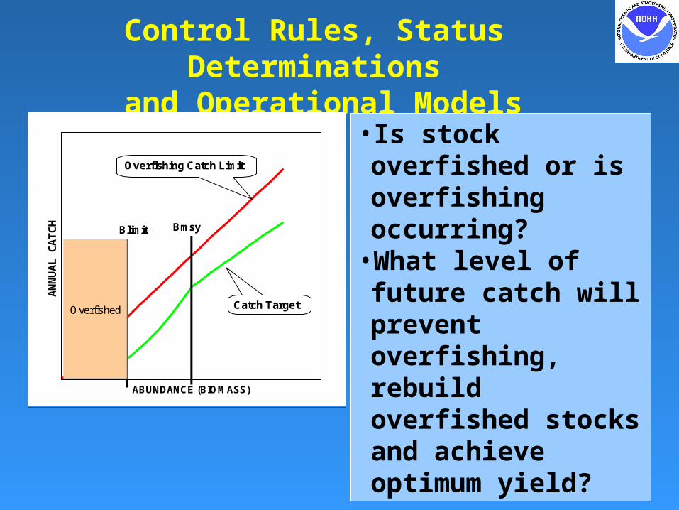
Control Rules, Status Determinations

and Operational Models•Is stock overfished or is overfishing occurring?

•What level of future catch will prevent overfishing, rebuild overfished stocks and achieve optimum yield?

ABUNDANCE (BIOMASS)

AN

NU

AL

CA

TC

H

BmsyBlimit

Overfished

Overfishing Catch Limit

Catch Target

4

Stock Assessment Defined

• Simplest System–Link control rule to simple data-based indicator of trend in B or F

–Easy to communicate; assumptions are buried

–Hard to tell when you’ve got it wrong

–Hard to put current level in historical context

• Full Model– Estimate level,

trend and forecast for abundance and mortality to implement control rules

– Cross-calibrates data types

– Complex to review and communicate

– Bridges to integrated ecosystem assessment

Collecting, analyzing, and reporting demographic information to determine the effects of fishing on fish populations

5

Idealized Assessment System

• Standardized, timely, comprehensive data

• Standardized models at the sweet spot of complexity

• Trusted process thru adequate review of data and models

• Timely updates using trusted process

• Clear communication of results, with uncertainty, to clients

6

POPULATION MODEL:(Abundance, mortality)

POPULATION MODEL:(Abundance, mortality)

STOCK STATUSSTOCK STATUS OPTIMUM YIELD

OPTIMUM YIELD

CATCHRETAINED AND

DISCARDED CATCH;AGE/SIZE DATA

BIOLOGY NATURAL MORTALITY,

GROWTH, REPRODUCTION

ABUNDANCE TREND RESOURCE SURVEY

or FISHERY CPUE,AGE/SIZE DATA

ADVANCED MODELS HABITAT CLIMATE ECOSYSTEM MANMADE STRESS

SOCIOECONOMICS

STOCK ASSESSMENT PROCESS

Conceptually like NOAA Weather’s data assimilation models, but time scale is month/year, not hour/day

7

Fish Biology and Life History

0 5 10 15 20 25

AGE

Length

Weight

Eggs

0.0

0.1

0.2

0.3

0.4

0.5

0.6

0.7

0.8

0.9

1.0

0 5 10 15 20 25

AGE

% Mature

Natural Mortality

Ease: Length & Weight >> Age > Eggs & Maturity >>> Mortality

8

Abundance IndexFishery-Independent Surveys

9

Source of Abundance Indexes

Each survey may support multiple assessmentsEach assessment may use data from multiple surveys

Catch: What’s Been Removed

• Must account for all fishing mortality– Commercial and recreational– Retained and discarded– Discard survival fraction

• Model finds F that matches observed catch given estimated population abundance– Because catch is nearly always the most

complete and most precise of any other data in the model

– But also possible to treat catch as a quantity that is imprecise and then to estimate F as a parameter taking into account the fit to all types of data

10

Catch Components

• Commercial retained catch– fish ticket census

• Commercial discard– observer program

• Recreational kept catch– catch/angler trip x N angler trips

• Recreational releases– Interview x N angler trips

11

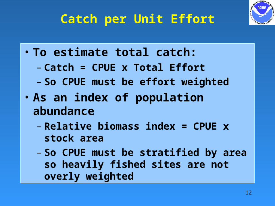
Catch per Unit Effort

• To estimate total catch:– Catch = CPUE x Total Effort– So CPUE must be effort weighted

• As an index of population abundance– Relative biomass index = CPUE x

stock area– So CPUE must be stratified by area

so heavily fished sites are not overly weighted

12

13

Integrated Analysis Models

• Population Model – the core

– Recruitment, mortality, growth

• Observation Model – first layer

– Derive Expected Values for Data

• Likelihood-based Statistical Model – second layer

– Quantify Goodness-of-Fit

• Algorithm to Search for Parameter Set that Maximizes the Likelihood

• Cast results in terms of management quantities

• Propagate uncertainty in fit onto confidence for management quantities

Stock Synthesis History

• Anchovy synthesis (~1985)• Generalized model for west coast

groundfish (1988)• Complete re-code in ADMB as SS2

(2003)• Add Graphical Interface (2005)• SS_V3 adds tag-recapture and

other features (2009)

14

15

Age-Length Structured Population

60

52

46

40

34

28

22

16

10

1

3

5

7

9

11

13

15

17

20

22

SIZE

AGE

POPULATION

0.0

0.2

0.4

0.6

0.8

1.0

25 30 35 40 45

SIZE

SE

LE

CT

IVIT

Y

16

Sampling & Observation Processes

60

52

46

40

34

28

22

16

10

1

3

5

7

9

11

13

15

17

19

21

23

SIZE

AGE

CATCH AT TRUE AGE

60

52

46

40

34

28

22

16

10

1

3

5

7

9

11

13

15

17

19

21

23+

SIZE

AGE'

CATCH-AT-OBSERVED "AGE"

With size-selectivity

And ageing imprecision

17

Expected Values for Observations

10 20 30 40 50 60

SE

LE

CT

IVIT

Y

SIZE

10 20 30 40 50 60

FR

EQ

UE

NC

Y

SIZE

POPULATIONCATCH

0 5 10 15 20 25

FR

EQ

UE

NC

Y

AGE

POPULATION

CATCH AT TRUE AGE

CATCH AT OBSERVED AGE

0 5 10 15 20 25

SIZ

E-A

T-A

GE

AGE

SIZE-at-TRUE AGE (population)

SIZE-at-TRUE AGE (catch)

SIZE-at-OBS AGE (catch)

18

Discard & Retention

0.0

0.5

1.0

0.00

0.02

0.04

0.06

0.08

0.10

0.12

0 20 40 60 80 100

Re

ten

ton

Fre

qu

en

cy

Size

Retained-obs

Retained-est

Discard-obs

Discard-est

Frac. Retained

19

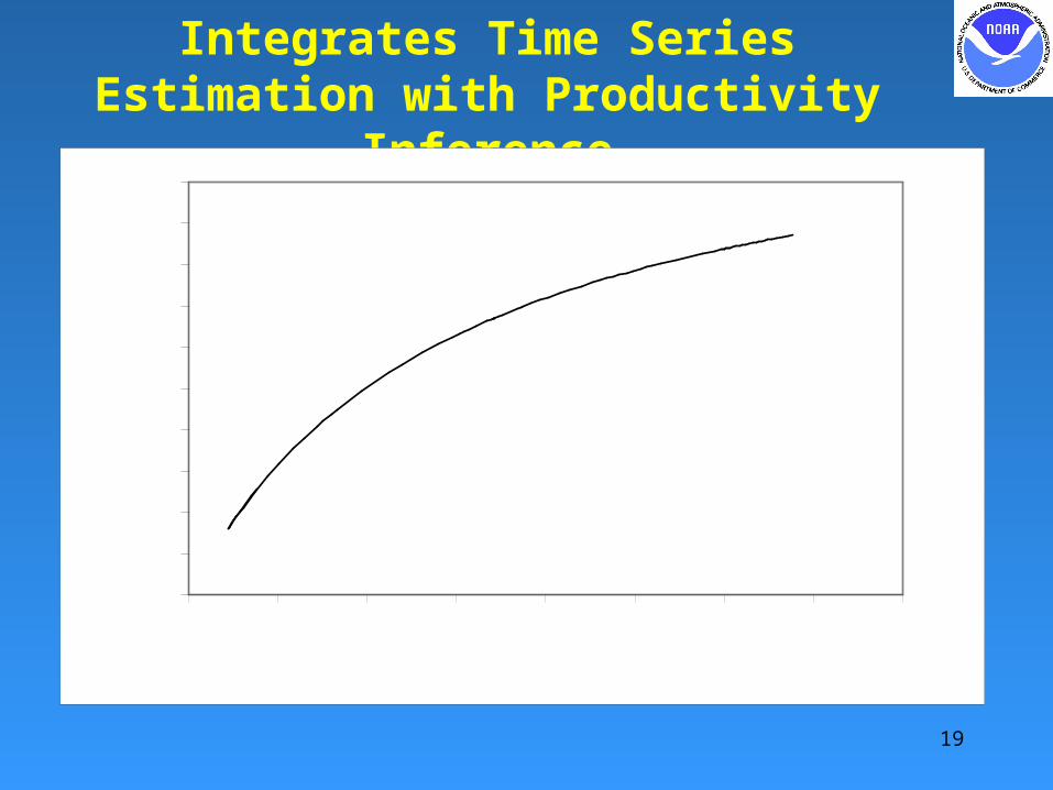
Integrates Time Series Estimation with Productivity

Inference

0

500

1000

1500

2000

2500

3000

3500

4000

4500

5000

0 5000 10000 15000 20000 25000 30000 35000 40000

Female Spawning Biomass

Rec

ruit

men

t

ExpectedBias-adjustTime_seriesVirgin & Init

20

Integrated Analysis

• Produces comprehensive estimates of model uncertainty

• Smoothly transitions from pre-data era, to data-rich era, to forecast

• Stabilizing factor:– Continuous population dynamics process

0

5000

10000

15000

20000

25000

30000

35000

40000

1950 1970 1990 2010YEAR

Biomass

Forecast

Catch DataOnly

0

5000

10000

15000

20000

25000

30000

35000

40000

45000

50000

1950 1970 1990 2010YEAR

Recruitment

21

AREAAge-specific movement between areas

FLEET / SURVEYLength-, age-, gender selectivity

NUMBERS-AT-AGECohorts: gender, birth season, growth pattern;“Morphs” can be nested within cohorts to achieve size-survivorship;Distributed among areas

RECRUITMENTExpected recruitment is a function of total female spawning biomass;Optional environmental input;apportioned among cohorts and morphs;Forecast recruitments are estimated, so get variance

Stock Synthesis Structure

CATCHF to match observed catch;Catch partitioned into retained and discarded, with discard mortality

PARAMETERSCan have prior/penalty;Time-vary as time blocks, random annual deviations, or a function of input environmental data

22

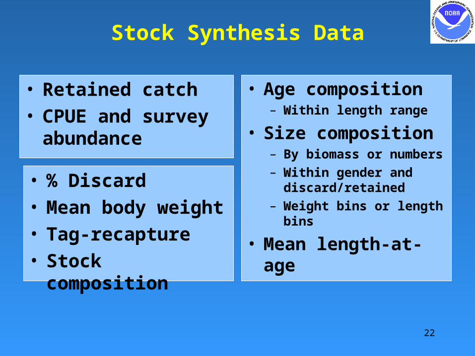
Stock Synthesis Data

• Retained catch• CPUE and survey

abundance

• Age composition– Within length range

• Size composition– By biomass or numbers– Within gender and

discard/retained– Weight bins or length

bins

• Mean length-at-age

• % Discard• Mean body

weight• Tag-recapture• Stock

composition

23

Variance Estimation

• Inverse Hessian (parametric quadratic approximation)

• Likelihood profiles• MCMC (brute force, non-

parametric)• Parametric bootstrap

24

Risk Assessment

– Calculate future benefits and probability of overfishing and stock depletion as a function of harvest policy for each future year

– Accounting for:•Uncertainty in current stock abundance•Variability in future recruitment•Uncertain estimate of benchmarks•Incomplete control of fishery catch•Time lag between data acquisition and mgmt revision

•Model scenarios•retrospective biases•Pr(ecosystem or climate shift)•Impacts on other ecosystem components

ADMB

• Auto-Differentiation Model Builder

• C++ overlay developed by Dave Fournier in 1980s

• Co-evolved with advancement of fishery models

• Recently purchased by Univ Cal (NCEAS) using a private grant

• Now available publically and will become open source software

25

Graphical Interface: Toolbox

26

27

Stock Synthesis Overview• Age-structured simulation model of population

– Recruitment, natural and fishing mortality, growth

• Observation sub-model derives expected values for observed data of various kinds and is robust to missing observations– Survey abundance, catch, proportions-at-age or length

• Can work with limited data when flexible options set to mimic simplifying assumptions of simple models

• Can include environmental covariates affecting population and observation processes

0

20000

40000

60000

80000

100000

120000

140000

160000

180000

200000

1974 1984 1994 2004

YEAR

SU

RV

EY

BIO

MA

SS

OBS +- 2 se

PREDICT

FISHERY AGE COMP in 1995

1 2 3 4 5 6 7 8 9 10 11 12 13 14 15-19

20-24

25+

AGE

FR

AC

TIO

N

OBSERVE

PREDICT

An Example

• Simple vs. complex model structure

• Time-varying model parameter• First, motivation for an

advanced approach to catchability

28

29

Calibrating Abundance Index

•The observed annual abundance index, Ot, is basically density (CPUE) averaged over the spatial extent of the stock

•Call model’s estimate of abundance, At

•In model: E(Ot) = q x At + e•Where q is an estimated model parameter•Concept of q remains the same across a range of data scenarios:

30

Calibrating Abundance Index

•If O time series comes from a single Fisheries Survey Vessel

•If survey vessel A replaces survey B and a calibration experiment is done

•If O come from four chartered fishing vessels each covering the entire area

•If O come from hundreds of fishing vessels using statistical model to adjust for spatial and seasonal effort concentration

31

Abundance Index Time Series

•Each set-up is correct, but what’s wrong with the big picture?

•q is not perfectly constant for any method!

•Some methods standardize q better than others

•Building models that admit the inherent variability in qt and constrain q variability through information about standardization and calibration can:

– achieve a scalable approach across methods;

– incorporate q uncertainty in overall C.I.;– Show value of calibration and

standardization

Example

• Fishery catch• CPUE, CV=0.1,

density-dependent q

• Triennial fishery-independent survey, CV=0.3

• Age and size composition, sample size = 125 fish

32

1970 1980 1990 2000

Catch

Survey

Fishery_CPUE

Results:all data, all parms, random walk

q

0.0

0.1

0.2

0.3

0.4

1970 1990 2010YEAR

F. Mort

0

2000

4000

6000

8000

10000

12000

1970 1990 2010YEAR

Catch

0

5000

10000

15000

20000

25000

30000

35000

40000

1950 1970 1990 2010YEAR

Biomass

Forecast

Catch DataOnly

0

5000

10000

15000

20000

25000

30000

35000

40000

45000

50000

1950 1970 1990 2010YEAR

Recruitment

Blue line = true values; red dot = estimate with 95% CI

Fishery q

34

0.0

0.5

1.0

1.5

2.0

2.5

3.0

3.5

4.0

1975 1985 1995

CATC

HA

BILI

TY (q

)

YEAR

True q

Random walk estimated q

CPUE only, Simple Model, constant q

0.0

0.1

0.2

0.3

0.4

1970 1990 2010YEAR

F. Mort

0

2000

4000

6000

8000

10000

12000

14000

1970 1990 2010YEAR

Catch

0

10000

20000

30000

40000

50000

60000

70000

80000

1950 1970 1990 2010YEAR

Biomass

Forecast

Catch DataOnly

0

5000

10000

15000

20000

25000

30000

35000

1950 1970 1990 2010YEAR

Recruitment

Bias and Precision in Forecast Catch

36

0

2000

4000

6000

8000

10000

12000

14000

TRUE All data, all parm, randwalk

All data, all parm,

constant q

Only CPUE, all parms,

constant q

Only CPUE, few parm, equil recr, constant q

Catc

h in

200

1

Error bar is +/- 1 std error

NEXT STEPS

• Tier III Assessments– Spatially explicit– Linked to ecosystem processes

37

38

Space: The Final Frontier

• “Unit Stock” paradigm:– Sufficient mixing so that localized

recruitment and mortality is diffused throughout range of stock

– Spatially explicit data is processed to stock-wide averages

• Marine Protected Area paradigm:– Little mixing so that protected fish stay

protected• Challenge: Implement spatially

explicit assessment structure with movement and without bloating data requirements

39

OPTIMUM YIELD

OPTIMUM YIELD

SINGLE SPECIESASSESSMENT

MODELTactical

TIME SERIESOF RESULTS

BIOMASS,RECRUITMENT,

GROWTH,MORTALITY

Stock Assessment – Ecosystem Connection

INTEGRATEDECOSYSTEM

ASSESSMENT CUMULATIVE EFFECTS OF

FISHERIES AND OTHER FACTORS

Strategic

INDICATORS ENVIRONMENTAL,ECOSYSTEM,OCEANOGRAPHIC

RESEARCH ONINDICATOR

EFFECTS

40

Getting to Tier III

Process Tier II Tier III

Average Productivity(Spawner-Recruitment)

Empirical over decades of fishing

Predict from Ecosystem Food Web and Climate Regimes

Annual RecruitmentAnnual random process with measurable outcome

Predictable from ecosystem and environmental factors

Growth & ReproductionMeasurable, but often held constant

Predictable from ecosystem and environmental factors

Survey CatchabilityUsually Constant or random walk

Linked to environmental factors

Natural MortalityMean level based on crude relationships and wishful thinking

Feasible?, or just wishful thinking on larger scale?

41

How Are We Doing?

YearAssessments

DoneStocks withAdeq. Asmt.

2000 37 1062001 53 1112002 64 1062003 60 1072004 63 1082005 105 1202006 68 1202007 74 128

Assessments of 230 FSSI stocks following SAIP and increased EASA funds

42

Summary

Stock Synthesis Integrated Analysis Model

• Flexible to accommodate multiple fisheries and surveys

• Explicitly models pop-dyn and observation processes (movement, ageing imprecision, size and age selectivity, discard, etc.)

• Parameters can be a function of environmental and ecosystem time series

• Estimates precision of results• Estimates stock productivity, MSY and

other management quantities and forecasts