STRUCTURAL AND MAGNETIC PROPERTIESOF RHODIUM CLUSTERS

SOON YEE YEEN

UNIVERSITI SAINS MALAYSIA

2016

STRUCTURAL AND MAGNETIC PROPERTIESOF RHODIUM CLUSTERS

by

SOON YEE YEEN

Thesis submitted in fulfilment of the requirementsfor the degree of

Master of Science

November 2016

ACKNOWLEDGEMENT

I would first like to express my deep gratitude to my supervisor, Dr. Yoon Tiem

Leong, for his professional guidance and suggestions throughout the period of this

project and thesis writing. Although he allows this project to be my own work, he helps

me to get into a right direction whenever I need help.

I would also like to sincerely thank Dr. Lim Thong Leng from Faculty of Engineering

and Technology, Multimedia University. He is my co-supervisor and the second reader

of this thesis. His constant encouragement and professional comments are utmost

helpful.

I would like to acknowledge the collaborating group, lead by Prof. Lai San Kiong

from Department of Physics of National Central University in Taiwan. Besides support-

ing me to have a one-month research visit in Taiwan, Prof. Lai and his fellow student

(Dr. Yen Tsung Wen) have provided consistent academic support and computational

tools to me throughout this period of study.

I am gratefully indebted to Dr. Francesca Baletto from Physics Department of

King’s College London for accepting me as a short-term visiting research student. She

and her group members (Prof. Roberto D’Agosta, Dr. Gian Giacomo Asara and Mr.

Kevin Rossi) generously share their valuable experiences and computational resources

with me so that I could learn new techniques that might be useful in the future.

I would like to thank my fellow colleagues from theoretical and computational

group for giving support in this research period. I have been input with new scientific

knowledge due to high commitment of the group to conduct monthly sharing session.

Thanks to Ms. Ong Yee Pin, who always provides me full encouragement throughout

ii

the period. Special thanks to Mr. Ng Wei Chun and Mr. Goh Eong Sheng, who have

helped me to solve all kinds of operational and technical problems that I faced while

carrying out this project.

Finally, I must express my very profound gratitude to my parents and to my friends

for providing me with continuous encouragement throughout my years of study. This

accomplishment would not have been possible without their unfailing support. Thank

you.

iii

TABLE OF CONTENTS

Acknowledgement . . . . . . . . . . . . . . . . . . . . . . . . . . . . . . . . . . . . . . . . . . . . . . . . . . . . . . . . . . . . . . . . . . . . ii

Table of Contents . . . . . . . . . . . . . . . . . . . . . . . . . . . . . . . . . . . . . . . . . . . . . . . . . . . . . . . . . . . . . . . . . . . . . iv

List of Tables . . . . . . . . . . . . . . . . . . . . . . . . . . . . . . . . . . . . . . . . . . . . . . . . . . . . . . . . . . . . . . . . . . . . . . . . . vii

List of Figures . . . . . . . . . . . . . . . . . . . . . . . . . . . . . . . . . . . . . . . . . . . . . . . . . . . . . . . . . . . . . . . . . . . . . . . . viii

List of Abbreviations . . . . . . . . . . . . . . . . . . . . . . . . . . . . . . . . . . . . . . . . . . . . . . . . . . . . . . . . . . . . . . . . . x

List of Symbols . . . . . . . . . . . . . . . . . . . . . . . . . . . . . . . . . . . . . . . . . . . . . . . . . . . . . . . . . . . . . . . . . . . . . . . xii

Abstrak . . . . . . . . . . . . . . . . . . . . . . . . . . . . . . . . . . . . . . . . . . . . . . . . . . . . . . . . . . . . . . . . . . . . . . . . . . . . . . . . xv

Abstract . . . . . . . . . . . . . . . . . . . . . . . . . . . . . . . . . . . . . . . . . . . . . . . . . . . . . . . . . . . . . . . . . . . . . . . . . . . . . . . xvii

CHAPTER 1 – INTRODUCTION . . . . . . . . . . . . . . . . . . . . . . . . . . . . . . . . . . . . . . . . . . . . . . . 1

1.1 Problem Statements . . . . . . . . . . . . . . . . . . . . . . . . . . . . . . . . . . . . . . . . . . . . . . . . . . . . . . . . . . . 2

1.2 Objectives of Study . . . . . . . . . . . . . . . . . . . . . . . . . . . . . . . . . . . . . . . . . . . . . . . . . . . . . . . . . . . . 3

1.3 Organization of Thesis . . . . . . . . . . . . . . . . . . . . . . . . . . . . . . . . . . . . . . . . . . . . . . . . . . . . . . . . 3

CHAPTER 2 – LITERATURE REVIEW . . . . . . . . . . . . . . . . . . . . . . . . . . . . . . . . . . . . . . 6

2.1 Overview of Nanoparticles . . . . . . . . . . . . . . . . . . . . . . . . . . . . . . . . . . . . . . . . . . . . . . . . . . . . 6

2.2 Magnetism of Nanoparticles . . . . . . . . . . . . . . . . . . . . . . . . . . . . . . . . . . . . . . . . . . . . . . . . . . 10

2.3 Works Related to Rhodium Clusters . . . . . . . . . . . . . . . . . . . . . . . . . . . . . . . . . . . . . . . . . . 13

CHAPTER 3 – THEORETICAL BACKGROUND . . . . . . . . . . . . . . . . . . . . . . . . . . . 17

3.1 Computational Modelling Techniques. . . . . . . . . . . . . . . . . . . . . . . . . . . . . . . . . . . . . . . . 17

3.2 Many-Body Gupta Potential . . . . . . . . . . . . . . . . . . . . . . . . . . . . . . . . . . . . . . . . . . . . . . . . . . 19

3.3 Optimisation Techniques . . . . . . . . . . . . . . . . . . . . . . . . . . . . . . . . . . . . . . . . . . . . . . . . . . . . . . 20

3.3.1 Basin Hopping . . . . . . . . . . . . . . . . . . . . . . . . . . . . . . . . . . . . . . . . . . . . . . . . . . . . . . . . 21

iv

3.3.2 Genetic Algorithm . . . . . . . . . . . . . . . . . . . . . . . . . . . . . . . . . . . . . . . . . . . . . . . . . . . . 22

3.3.3 Coupling of Basin Hopping and Genetic Algorithm . . . . . . . . . . . . . . . . 23

3.4 Density Functional Theory . . . . . . . . . . . . . . . . . . . . . . . . . . . . . . . . . . . . . . . . . . . . . . . . . . . . 26

3.4.1 The Schrödinger Equation . . . . . . . . . . . . . . . . . . . . . . . . . . . . . . . . . . . . . . . . . . . . 27

3.4.2 The Born-Oppenheimer Approximation . . . . . . . . . . . . . . . . . . . . . . . . . . . . . 30

3.4.3 Electon Density and The Thomas-Fermi Model. . . . . . . . . . . . . . . . . . . . . 31

3.4.4 The Hohenberg-Kohn Theorems . . . . . . . . . . . . . . . . . . . . . . . . . . . . . . . . . . . . . 32

3.4.5 The Kohn-Sham Approach . . . . . . . . . . . . . . . . . . . . . . . . . . . . . . . . . . . . . . . . . . . 34

3.4.6 Approximate Exchange-Correlation Functionals . . . . . . . . . . . . . . . . . . . . 37

3.4.7 Basis Sets . . . . . . . . . . . . . . . . . . . . . . . . . . . . . . . . . . . . . . . . . . . . . . . . . . . . . . . . . . . . . . 39

CHAPTER 4 – LOWEST-ENERGY CONFIGURATIONS OFRHODIUM CLUSTERS . . . . . . . . . . . . . . . . . . . . . . . . . . . . . . . . . . . . . . . 41

4.1 Computational Details. . . . . . . . . . . . . . . . . . . . . . . . . . . . . . . . . . . . . . . . . . . . . . . . . . . . . . . . . 41

4.2 Validation of Methodology: Rhodium Atom and Dimer . . . . . . . . . . . . . . . . . . . . 46

4.3 Optimized Configurations of Rhodium Clusters . . . . . . . . . . . . . . . . . . . . . . . . . . . . . 50

4.4 Conclusions . . . . . . . . . . . . . . . . . . . . . . . . . . . . . . . . . . . . . . . . . . . . . . . . . . . . . . . . . . . . . . . . . . . . 68

CHAPTER 5 – STRUCTURAL AND MAGNETIC PROPERTIES OFRHODIUM CLUSTERS . . . . . . . . . . . . . . . . . . . . . . . . . . . . . . . . . . . . . . . 70

5.1 Vibrational Frequency Analysis . . . . . . . . . . . . . . . . . . . . . . . . . . . . . . . . . . . . . . . . . . . . . . 70

5.2 Size-dependence Magnetism of Rhodium Clusters . . . . . . . . . . . . . . . . . . . . . . . . . . 76

5.3 Relative Stability of Rhodium Clusters. . . . . . . . . . . . . . . . . . . . . . . . . . . . . . . . . . . . . . . 78

5.4 Structural Properties . . . . . . . . . . . . . . . . . . . . . . . . . . . . . . . . . . . . . . . . . . . . . . . . . . . . . . . . . . . 81

CHAPTER 6 – ELECTRONIC STRUCTURES OF RHODIUMCLUSTERS . . . . . . . . . . . . . . . . . . . . . . . . . . . . . . . . . . . . . . . . . . . . . . . . . . . . . . 89

v

6.1 Molecular Orbitals. . . . . . . . . . . . . . . . . . . . . . . . . . . . . . . . . . . . . . . . . . . . . . . . . . . . . . . . . . . . . 89

6.1.1 Electronic Stability . . . . . . . . . . . . . . . . . . . . . . . . . . . . . . . . . . . . . . . . . . . . . . . . . . . . 95

6.2 Population Analysis . . . . . . . . . . . . . . . . . . . . . . . . . . . . . . . . . . . . . . . . . . . . . . . . . . . . . . . . . . . 96

6.2.1 Löwdin Populations . . . . . . . . . . . . . . . . . . . . . . . . . . . . . . . . . . . . . . . . . . . . . . . . . . . 97

6.2.2 Charge Distribution of Rhodium Clusters . . . . . . . . . . . . . . . . . . . . . . . . . . . 97

6.2.3 Spin Distribution of Rhodium Clusters . . . . . . . . . . . . . . . . . . . . . . . . . . . . . . 104

CHAPTER 7 – CONCLUSIONS AND FUTURE STUDIES . . . . . . . . . . . . . . . . . 110

7.1 Conclusions . . . . . . . . . . . . . . . . . . . . . . . . . . . . . . . . . . . . . . . . . . . . . . . . . . . . . . . . . . . . . . . . . . . . 110

7.2 Future Studies . . . . . . . . . . . . . . . . . . . . . . . . . . . . . . . . . . . . . . . . . . . . . . . . . . . . . . . . . . . . . . . . . 116

References . . . . . . . . . . . . . . . . . . . . . . . . . . . . . . . . . . . . . . . . . . . . . . . . . . . . . . . . . . . . . . . . . . . . . . . . . . . . 118

Appendices

Appendix A – Optimization At Empirical Level

A.1 Optimized Structures of Rhodium Clusters

Appendix B – Vibrational Frequency Analysis

B.1 Zero-point Energy

B.2 Infrared Spectra

vi

LIST OF TABLES

Page

Table 3.1 Atomic units 29

Table 4.1 Gupta potential parameters for Rh clusters. 42

Table 4.2 Validation of approach for the energy functional. 46

Table 4.3 Calculations of Rh2 with different basis sets. 48

Table 4.4 Summarized results on optimized configurations of Rh3. 51

Table 4.5 Summarized results on optimized configurations of Rh4. 52

Table 4.6 Summarized results on optimized configurations of Rh5. 53

Table 4.7 Summarized results on optimized configurations of Rh6. 54

Table 4.8 Summarized results on optimized configurations of Rh7. 55

Table 4.9 Summarized results on optimized configurations of Rh8. 56

Table 4.10 Summarized results on optimized configurations of Rh9. 57

Table 4.11 Summarized results on optimized configurations of Rh10. 58

Table 4.12 Summarized results on optimized configurations of Rh13. 60

Table 4.13 Summarized results on magnetism of optimized RhN (20≤N ≤ 23).

65

Table 5.1 Average binding energies of Rh clusters. 79

Table 5.2 Symmetry order. 85

Table A.1 Symmetry and binding energies of Rh clusters optimized atempirical level.

126

Table B.1 Zero-point energies of Rh clusters. 129

vii

LIST OF FIGURES

Page

Figure 2.1 Typical size of small particles. 7

Figure 2.2 Examples of cluster types. 8

Figure 2.3 Spin occupation in a cluster. 11

Figure 3.1 Example of PES. 18

Figure 3.2 Transformed PES from BH. 22

Figure 4.1 Variation of relative energy with spin multiplicity for clusterswith different sizes.

44

Figure 4.2 Optimized atomic structures of RhN (3≤ N ≤ 5). 50

Figure 4.3 Optimized atomic structures of RhN (6≤ N ≤ 8). 54

Figure 4.4 Optimized atomic structures of RhN (9≤ N ≤ 13). 57

Figure 4.5 Optimized atomic structures of RhN (14≤ N ≤ 19). 62

Figure 4.6 Optimized atomic structures of RhN (20≤ N ≤ 23). 64

Figure 4.7 Optimized atomic structures of RhN (N = 26,30,38). 66

Figure 5.1 A transition state and a minimum on a potential energy sur-faec.

74

Figure 5.2 Variation of relative energy with spin multiplicity for Rh13cluster.

75

Figure 5.3 Average magnetic moment of Rh clusters against cluster size. 77

Figure 5.4 Dissociation energy and second-order difference of total en-ergies against cluster size.

80

Figure 5.5 Average binding energies and average radial bond distancesagainst cluster size.

82

Figure 5.6 Average nearest-neighbour distance of Rh clusters againstcluster size.

83

viii

Figure 5.7 Average magnetic moment and symmetry order of Rh clustersagainst cluster size.

87

Figure 6.1 Occupation of spins in restricted and unrestricted formalism. 90

Figure 6.2 Spin occupation in Rh atom. 93

Figure 6.3 Spin occupation in Rh dimer. 94

Figure 6.4 HOMO-LUMO gaps of rhodium (Rh) clusters against clustersize.

95

Figure 6.5 Charge distribution of optimized Rh clusters. 100–103

Figure 6.6 Spin distribution of optimized Rh clusters. 106–109

Figure A.1 Optimized structures of Rh clusters at empirical level. 127–128

Figure B.1 Infrared spectra of Rh clusters. 130–133

ix

LIST OF ABBREVIATIONS

Ag silver

Au gold

BFGS Broyden–Fletcher–Goldfarb–Shanno

BH basin hopping

BHGA basin hopping plus genetic algorithm

BO Born-Oppenheimer approximation

bcc body-centered cubic

Co cobalt

Cu copper

DFT density functional theory

DFTB density functional based tight binding

ECP effective core potential

Fe iron

fcc face-centered cubic

GA genetic algorithm

GGA generalized gradient approximation

GTO Gaussian-type-orbitals

HF Hartree-Fock

HOMO highest occupied molecular orbital

KS Kohn-Sham

LCAO linear combinations of atomic orbitals

LCGTO linear combination of Gaussian-type orbital

LDA local-density approximation

LUMO lowest unoccupied molecular orbital

MCP model core potential

Ni nickel

PES potential energy surface

Pd palladium

x

PT parallel tempering

Pt platinum

PTMBHGA parallel tempering multicanonical basin hopping plus genetic algorithm

QECP quasi-relativistic effective core potential

RMCP relativistic model core potential

RMS root mean square

SCF self-consistent field

SK Slater-Koster

Rh rhodium

TF Thomas-Fermi

xi

LIST OF SYMBOLS

α up spin

β down spin

ρ electron density

µ total spin magnetic moment

ν vibrational frequency

η basis function

χ spin orbital

ϕ spatial orbital

ε energy of spin orbital

ε0 vacuum dielectric constant

Ψ wavefunction

Ψelec electronic wavefunction

ν random number in GA

φ sorting parameter in GA

δ space between stationary energy levels

N cluster size (number of atoms)

n number of electrons

Nc number of individuals (atomic configurations)

Nq number of charges

e charge of an eletron

Z charge of a nucleus

m mass of a nucleus

me mass of an electron

mr reduced mass

R or r position vector

s position vector of a charge

ri j pair distance between atoms i and j

r0 nearest-neighbour distance

xii

d average radial bond distance

P momentum of a nucleus

p momentum of an electron

M spin multiplicity

M total spin angular momentum

H Hamiltonian operator

Helec electronic Hamiltonian operator

f normalized fitness in GA

C any configuration

CTF constant for TF model

g gradient matrix

H Hessian (force constant matrix)

k force constant of a vibration mode

E energy

EF Fermi energy

Eb binding energy

Etot total energy

Eelec total electronic energy

Ekin total kinetic energy

Exc exchange-correlation energy

ETF energy of an atom in TF model

TTF kinetic energy in TF model

∆E relative energy with respect to lowest energy level

∆2E second-order difference of energies

De dissociation energy

J Coulomb repulsion

V potential energy of opriginal PES in BH

V potential energy of transformed PES in BH

Vrep repulsive potential in Gupta potential

xiii

Vatt attractive potential in Gupta potential

VNe attractive potential ecerted by nuclei on electrons

Vxc exchange-correlation potential

Vext external potential

Veff external potential in KS approach

xiv

SIFAT-SIFAT STRUKTUR DAN MAGNETIK KLUSTER RHODIUM

ABSTRAK

Kluster nano merupakan satu sistem yang amat menarik sejak dekad akhir-akhir ini

kerana, jika dibandingkan dengan keadaan pukal, ia memperlihatkan kelakaun yang

pelik di mana sifat-sifat tabiinya bergantung kepada saiz. Setakat unsur-unsur peralihan

4d dipertimbangkan, kluster rhodium (Rh) merukapan salah satu sistem yang paling

banyak diperbahaskan. Rh dalam bentuk pukal adalah bahan paramagnet, tetapi apabila

ia dikurangkan kepada dimensi berskalar atomik, sifat-sifat struktur dan magnetiknya

akan berubah-ubah mengikuti saiz kluster. Projek ini bertujuan untuk mengaji dan

menyiasat secara sistematik sifat-sifat yang pelik tersebut bagi kluster RhN yang berada

pada keadaan tenaga yang paling rendah, di mana N adalah bilangan atom di antara

2 hingga 23. Untuk melanjutkan pemahaman dalam kluster-kluster yang besar, Rh26,

Rh30 dan Rh38 juga termasuk dalam kajian tersebut. Konfigurasi kluster-kluster pada

keadaan tenaga yang paling rendah diperolehi dengan menjalankan pengoptimuman

berperingkat dua. Mula-mula sekali, satu konfigurasi rawak dioptimumkan secara global

dengan menggunakan satu algoritma carian yang tidak berat sebelah, BHGA (keupayaan

empirikal Gupta sebagai kalkulator tenaga), diikuti dengan pengoptimuman secara lokal

melalui pengiraan berprinsip pertama DFT dengan formalisma spin-polarisasi LCAO.

Struktur-struktur yang telah dioptimum tersebut juga tertakluk kepada analisis frekuensi

getaran untuk menyingkirkan keadaan-keadaan peralihan yang tidak stabil. Kestabilan

relatif dan sifat-sifat struktur kluster-kulster Rh yang telah dioptimum juga dikaji

dengan menjalankan analisis energik dan pengiraan daripada aspek geometri. Sifat-

xv

sifat magnet yang bergantung kepada saiz kluster adalah dibentangkan dan dikaitkan

dengan faktor geometri. Struktur elektronik kluster-kluster Rh juga dikaji supaya dapat

memahami dengan lebih lanjut mengenai bagaimana elektron ditaburkan dalam struktur-

struktur kluster malalui analisis populasi. Secara umum, hasil kajian ini bersetuju

dengan kerja-kerja lain yang dilaporkan sebelum ini. Hasil-hasil baru yang diperoleh

dalam tesis ini termasuk (i) konfigurasi yang telah dioptimum bagi kluster-kluster besar

yang jarang dilaporkan seperti Rh26, Rh30 dan Rh38, (ii) kluster-kluster Rh menjadi

lemah dalam magnetik apabila bilangan atom melebihi 19, serta (iii) order makgetik

yang luar jangkaan dalam beberapa kluster didedahkan, di mana spin-spin negatif

dijumpai dalam atom-atom terpilih dalam kluster-kluster tersebut. Khususnya, tesis

ini meramalkan anomali momen magnet yang besar untuk Rh38, pada nilai 30 µB,

yang tidak pernah dilaporkan dalam literatur. Projek tesis juga melaporkan satu hasil

kajian yang sistematik untuk pemodelan komputasi bagi kluster Rh pada peringkat

atomik dengan menggunakan strategi komputasi berperingkat dua dan pelbagai perkakas

teori. Perkakas-perkakas tersebut termasuk algoritma carian global yang berkuasa,

kalkulator tenaga keupayaan empirikal, DFT untuk pengoptimuman lokal, pengiraan

struktur elektronik serta analisis frekuensi getaran. Metodologi dan strategi pengiraan

kajian ini pada dasarnya boleh diaplikasikan pada sistem-sistem nano yang lain untuk

memperolehi pemahaman yang berharga pada tahap DFT.

xvi

STRUCTURAL AND MAGNETIC PROPERTIES OF RHODIUM CLUSTERS

ABSTRACT

Nanocluster has been a system of interest for the past decades due to its peculiar

size-dependent properties as compared to its bulk counterparts. As far as 4d transition

elements are concerned, rhodium (Rh) cluster is one of the most-debated systems.

Bulk Rh is a paramagnetic material, but when it is reduced to atomic dimension, its

structural and magnetic properties vary with the cluster size. This project is aimed

to perform systematic study to investigate the unusual properties at the lowest energy

state of RhN clusters, where N is the number of atoms ranged from 2 to 23. To further

understandings in large clusters, Rh26, Rh30 and Rh38 are also included in the study.

The lowest-energy configurations of the clusters are obtained by performing two-stage

optimization. A random configuration is first globally optimized using an unbiased

search algorithm, BHGA (empirical Gupta potential as energy calculator), followed

by locally optimized via first-principles DFT calculations with spin-polarized LCAO

formalism. The optimized structures are also subjected to vibrational analysis to rule

out transitional states which are not stable. Relative stabilities and structural properties

of the optimized Rh clusters are also studied by performing energetic analysis and

calculations from geometrical aspects. Size-dependence magnetic properties of the

clusters are presented and related to the geometrical factor. Electronic structures of

Rh clusters are studied to further understand how are the electrons distribute over the

structures via population analysis. In general, the results from current study agree

with previous works. The new results obtained in this thesis include (i) optimized

xvii

configurations of larger clusters that are rarely reported previously such as Rh26, Rh30

and Rh38, (ii) Rh clusters become weakly magnetic when the number of atoms exceeds

19, and (iii) unexpected magnetic ordering in some clusters are revealed, in which

negative spins are found in selected atoms in these clusters. In particular this thesis

predicts an anomalously large total magnetic moment for Rh38 at a value of 30 µB, which

is not reported in the literature. This thesis reports a systematic study to computational

modelling of Rh clusters at atomistic level using a two-stage computational strategy and

multitude of theoretical tools. These tools include a powerful global search algorithm,

empirical potential energy calculator, DFT for local optimization, electronic structure

and vibrational analysis. The methodology and computational strategy used in this work

can be in principle applied to other cluster systems to gain valuable DFT-level insight

of other nanosystems.

xviii

CHAPTER 1

INTRODUCTION

Why can’t we manufacture these small computers somewhat like we manufacture

the big ones? What are the limitations as to how small a thing has to be before you can

no longer mold it? - Feynman (1960) -

It has been decades after the early concept of miniaturization is introduced, yet its

development does not arrive at the saturation stage. In fact, engineers and researchers are

still trying to manufacture ever smaller electronic, optical and mechanical devices. The

greatest motivation of developing nanotechnology is due to its wide range of promising

technological applications, from industrial (as in catalytic process) to medical (as in

cancer diagnosis) applications.

Nowadays, thanks to modern technological advances, experimentalists are able

to fabricate, manipulate and even visualize particles at the atomic scale, specifically

nanoparticles with diameters much less than 100 nm. On the other hand, with powerful

high-performance computing resources, theorists are able to suggest new insights,

investigate thoroughly properties and applications of nanoparticles, as well as design a

new material by carrying out in silico experiments. As a result of the synergy between

interdisciplinary experimental and theoretical point of views, material science in low

dimension is still the field of interest and worthwhile for further study.

As far as theoretical investigation is concerned, theorists have been studying a

1

variety of materials, including organic and inorganic materials, particularly the transition

elements. In previous studies, it has been shown that nanoclusters, especially for those

comprised of 3d and 4d transition elements, exhibit peculiar properties as compared

to their bulk counterparts. Despite the existence of many theoretical works to predict

ground-state structures of clusters, they are difficult to be confirmed experimentally

due to scarcity of experimental evidence. Among all, rhodium (Rh), which has great

applications in catalysis, is one of the most debated 4d transition elements.

1.1 Problem Statements

Although there have been a number of theoretical works reported on the unusual

size-dependent properties of Rh clusters, there are still unsettled inconsistency in the

results of such published studies mainly due to the lack of experimental evidence on

measured geometrical structures of the clusters.

Density functional theory (DFT) calculations of clusters are commonly categorised

into two types of formalisms, namely, plane-wave basis and linear combinations of

atomic orbitals (LCAO) approaches. It is generally agreed that the former is more

suitable for periodic systems meanwhile the latter is for finite systems. In the literature,

both formalisms have been used to calculate clusters at DFT level. Most of the previous

studies of Rh clusters based on LCAO formalism concentrates only on small clusters

(. Rh13). In addition, electronic structures and magnetic ordering of Rh clusters for

sizes larger than 13 using LCAO approach are also seldom reported in details.

2

1.2 Objectives of Study

This thesis is aspired to provide a detailed density functional theory (DFT) com-

putational study on the Rh clusters with a selected range of sizes measured in terms

of the number of atom comprising the clusters. The first objective of this study is to

determine the lowest-energy configurations of Rh clusters, up to 23 atoms. In addition

to that, clusters with 26, 30 and 38 atoms are selectively chosen for the study. This work

locates the global minimum of each cluster by performing a two-stage optimization:

(i) unbiased search for the lowest-energy structure of a cluster in the Gupta empirical

potential energy surface, and followed by (ii) optimization of the structures obtained

from (i) using first-principles DFT calculation.

The next objective is to derive the structural and magnetic properties of the DFT-

optimized Rh clusters, targeting large cluster sizes (N ≥ 20) that have rarely been

reported in the literature.

Last but not least, the present work endeavours to derive the very physically-pertinent

information of the electronic structures of the clusters, including their molecular orbitals,

distributions of charges and spins over the clusters, and hence, their magnetic orderings.

1.3 Organization of Thesis

Up to this point, a brief introduction about the motivation and objectives of this

thesis has been given in Sections 1.1 and 1.2.

The following chapter (Chapter 2) is separated into two major parts to review

available literature: (i) a general introduction of atomic clusters and magnetism of

3

nanoparticles, and (ii) previous works related to Rh clusters. In this chapter, it highlights

the gap in the theoretical understanding of Rh clusters, which becomes the motivation

of this project.

Chapter 3 discusses the theoretical frameworks that form the basis of the methods

employed in this project. It starts from the fundamental understanding in computational

modelling techniques, followed by the conventional optimization approaches to locate

the global minimum in a potential energy surface. The basic ideas and theoretical basis

of DFT are also covered in this chapter.

The methodology (computational details), including the computational protocol em-

ployed, parameters and approximations used in this project, is given in Chapter 4. Also,

the geometrical structures and associated magnetic moments of the DFT-optimized Rh

clusters obtained are reported. The results are then discussed and compared with that

reported in the literature.

Before proceeding to a more detailed calculation on the DFT-optimized Rh clus-

ters, the vibrational frequency analysis, which is performed to check whether a given

configuration is a true global minimum, is discussed in the first section of Chapter 5.

The unusual size-dependence magnetic properties of Rh clusters are displayed in the

following section. Following this, the optimized configurations are investigated from

energetic and geometrical aspects in order to study the structural properties of the Rh

clusters.

The electronic structures of the optimized Rh clusters are explored in Chapter 6. In

this chapter, molecular orbitals of the clusters are investigated in order to understand

4

the arrangement of electrons in spin-polarized environment. This is followed by the

discussion on the electronic stability of the clusters. Subsequently, the distributions of

charges and spins of the electrons over the clusters, which in turn suggest their magnetic

orderings, are discussed in this chapter.

Lastly, the thesis is concluded in Chapter 7. The chapter also gives suggestions

on how to improve the present computational modelling technique and other possible

directions as extensions to the work done in this thesis. This thesis presents two

appendices: Appendix A illustrates the optimized Rh clusters at empirical level, while

Appendix B displays displays the zero-point energies and infrared spectra of Rh clusters

optimized from DFT.

5

CHAPTER 2

LITERATURE REVIEW

This chapter gives an overview of nanoparticles. Next, optimization methods

generally used in theoretical frameworks are tabled, followed by topics related to

magnetism of nanoparticles. The last section reviews previous works, both theoretical

and experimental ones, that are related to rhodium (Rh) clusters.

2.1 Overview of Nanoparticles

Nanoscience has encountered vast development for the past decades following the

vision of Feynman (1960). This field is not only limited to the understanding of basic

sciences, but also involve new technological (Baletto & Ferrando, 2005). The materials

that are involved in these studies and applications are called nanomaterials. One of the

nanomaterials of great interest is nanoparticles, and they are ultra-fine particles in the

size of nanometer order (Nogi, Naito, & Yokoyama, 2012). Comparison with other

small particles whose sizes are below 1 mm is shown in Figure 2.1 (Roduner, 2006). In

general, nanoparticles can exist in various forms like spherical, rod-like, film or more

complex geometries.

Nanoparticles play an important role of being a bridge connecting atoms or molecules

and bulk materials. This is because these particles behave very much differently as

compared to their bulk counterparts. In fact the properties of nanoparticles, such as

structural, thermal and magnetic properties, change drastically with size. Such unusual

6

Figure 2.1: Comparison of the size of nanoparticles with other small particles. Thedimension of nanoparticles is in the regime below 0.1 µm.(Roduner, 2006)

size dependence has prompted much interest among researchers to provide theoretical

explanations and gather more in-depth experimental data to this phenomena, as well as

finding a way to control their properties by controlling their formation process (Baletto

& Ferrando, 2005).

On the other hand, what really interest engineers are the applications of nanoparticles.

Nanoparticles, especially nanoclusters, have a wide range of applications, including

skincare cosmetics, cancer treatment, light emitting diodes, microelectronics packaging

and etc. Nanoclusters not only can be used in homogeneous catalytic reactions, they

also valuable information in designing nanocatalysts with specific reactivity. In addition,

a variety of nanoparticles such as carbon nanotubes, metal and semiconductor nanoclus-

ters, have been synthesized and proposed as potential building blocks for optical and

electronic devices (Castleman Jr & Khanna, 2009; Fedlheim & Foss, 2001; Nogi et al.,

2012; Tsutsui, 2012).

Nanocluster (in short, cluster) is referred to a particle that aggregates between a few

and many millions of identical or various types of atoms or molecules, with size about

1 – 10 nm (Fedlheim & Foss, 2001; Ferrando, Jellinek, & Johnston, 2008). It can be in

7

Figure 2.2: Examples of cluster types: (a) fullerenes [C60 (T. Yen & Lai, 2015)], (b)metal clusters [Ag147 (Huang et al., 2011)], (c) ionic clusters [(NaCl)13Cl−(Doye &Wales, 1999)], and (d) molecular clusters [(H2O)16 (D. J. Wales & Hodges, 1998)].

different shapes, for example a sphere and a plane that are very symmetric or irregular

shape as in amorphous (Roduner, 2006). There are assorted types of clusters that have

been studied experimentally or through computer simulation, such as fullerenes, metal,

ionic and molecular clusters as illustrated in Figure 2.2 (Johnston, 2002). In contrast to

a simple molecule, a cluster does not have a fixed size or composition. For instance,

an oxygen and two hydrogen atoms are placed at a well-defined angle to each other

in a water molecule, whilst a water cluster may contain a number of water molecules,

binding together to form in overall a specific shape as displayed in Figure 2.2(d) (Baletto

& Ferrando, 2005). The most important feature that draws attentions from scientists and

engineers is their size-dependent properties, at which their geometric shape and energy

stability as well as electronic properties are drastically changed with size (Ferrando et

al., 2008). Hence, studying the clusters of chosen composition and size allows ones

to investigate their unique physical and chemical behaviour, as well as exploring the

8

fundamental mechanisms governing their chemical reactivity (Castleman Jr & Khanna,

2009).

The extensive studies in this field involve various types of material, which have

covered most of the elements in the periodic table, from alkali metals to late-transition

metals as well as non-metals and rare gases. Among all, metal clusters are the most

investigated because of their wide range of applications and the advantage of being com-

paratively easier to be synthesized and modified chemically (Fedlheim & Foss, 2001).

Attentions are especially drawn to the transition metals that have been proved to have

great industrial applications. Going down the transition block, clusters of ferromagnetic

3d elements like iron (Fe), cobalt (Co) and nickel (Ni) show enhancement in magnetic

moments and this is found to be caused by the increase in localization of electrons

and their narrow band widths (Billas, Chatelain, & de Heer, 1994). On the other hand

in period 5 and 6, 4d and 5d elements are non-magnetic in bulk form. However, 4d

metal like rhodium (Rh) and palladium (Pd), and 5d metal like platinum (Pt) become

magnetic when their dimensions are reduced to atomic scale (Cox, Louderback, Apsel,

& Bloomfield, 1994; Di Paola, D’Agosta, & Baletto, 2016; Kumar & Kawazoe, 2003).

The clusters composed of coinage metal from group 11, especially the copper (Cu),

silver (Ag) and gold (Au), are of great interests to researchers. In particular, Au cluster

draws the most attention as it has been reported for transformation from a planar struc-

ture to a three-dimensional structure (Xiao & Wang, 2004) when it arrives at certain

number of atoms.

Apart from pure metal clusters, there are also vast studies in nanoalloys, comprised

of more than one type of atoms. Ferrando et al. (2008) reviewed different kind of works

9

related to bimetallic cluster, from experimental techniques for generating and character-

izing the nanoalloys to theoretical studies of their geometrical and dynamical properties.

Works also have been extended to ternary clusters, and they are more complex compared

to pure metal and bimetallic clusters in terms of interatomic interactions, and hence

searching of their ground-state configurations is a nightmare. One of the most-studied

clusters is Cu-Ag-Au. It has been fabricated by physical vapour deposition (Chatterjee,

Howe, Johnson, & Murayama, 2004). Its segregation is later studied by computational

modelling at the empirical level by using different methods (Cheng, Liu, Wang, & Huan,

2007; Liu, Espinosa-Medina, Sosa, & la Torre, 2009; Wu, Wu, Chen, & Qiao, 2011).

Nanoparticles have great potentials for advanced applications. Theoretical study

is as important as fabrication and synthesis of the nanoparticles, as it allows one to

peek more fundamentally into the size-dependence of the clusters. It allows ones to

understand the transformation of the properties as the system grows, which in turn can

be references for the experimentalists and engineers for further applications in real life.

2.2 Magnetism of Nanoparticles

Magnetism, due to its wide application in practice, is one of the most interested and

important properties for a given material. Magnetic property is widely applied has been

greatly contributing in medical fields, including the magnetic resonance imaging (MRI),

cancer treatment and targeted drug delivery. The concept of magnetism is also used

in environmental treatment, in which the contaminants are seperated from a solution

through the use of an external magnetic field (Binns, 2014). Nowadays, the development

of new technological processes permits the production of smaller magnetic particles, as

10

Figure 2.3: Schematic representation of the spin occupation of a set of equally spacedlevels in a cluster (de Jongh, 2013).

they are used in increasing information density in data storage (Roduner, 2006). These

are the practical motivations that make magnetism of nanoparticles a continual hot

research topic.

Assume that a cluster has reached equilibrium, and its stationary energy levels as

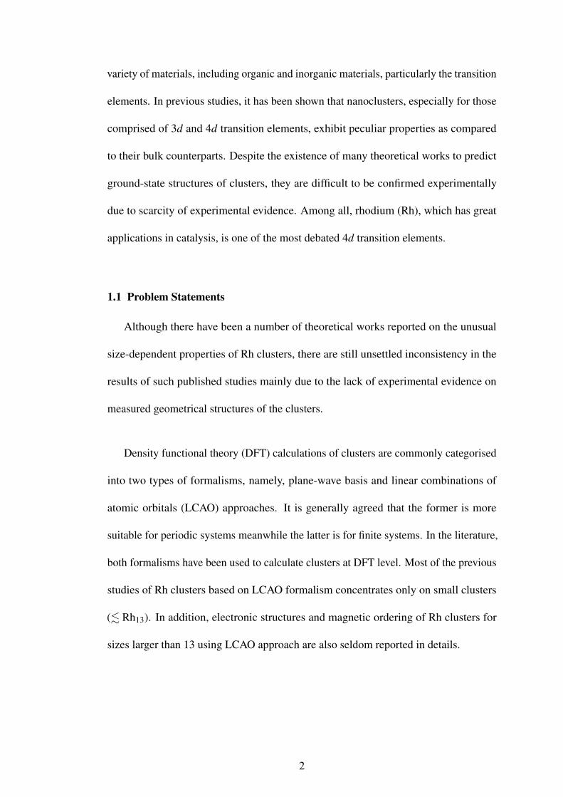
obtained from Hamiltonian are equally spaced with δ , is shown in Figure 2.3. The

n electrons start occupying the energy levels until they arrive at the last and highest

level, the Fermi energy (EF). It is shown that for an even number of n, there are two

electrons with opposite spins occupied at EF, cancelling each other and resulted in a

non-magnetic cluster. On the other hand, when n is odd, there is an unpaired spin at EF

which makes the cluster magnetic (de Jongh, 2013).

There are two main factors that contribute to the magnetic behaviour of magnetic

clusters, namely intra-atomic and interatomic charge transfer (Di Paola et al., 2016). The

intra-atomic charge transfer is induced by the intraband splitting between up and down

spins around EF. Tsukerblat (2008) have discussed the group-theoretical approaches

based on the spin and point symmetries which might results in molecular magnetism in

11

metal clusters. On the contrary, the interatomic contribution indicates the charge transfer

between adjacent atoms. In other words, it depends on the immediate environment

of the atoms which relates directly to the geometrical structure of the cluster itself

(Roduner, 2006).

The local geometrical environment has been shown to be one of the factors that

dominates the magnetism of metal clusters. For instance, local dimensionality and

structural symmetry might enhance or reduce magnetic effect of a cluster. In this

respect, Dunlap (1990) has linked the structural symmetry to the magnetism of 13-atom

Fe clusters, suggesting high-symmetrical icosahedral structure with greatest magnetic

moments is the ground-state configuration. It is suggested that the clusters with high

symmetry are more likely to have a multiply degenerate ground state. The degeneracy

allows different spins to occupy the orbitals according to Hund’s rule which promotes

more unpaired spins and hence, each atom is expected to carry a larger magnetic moment

(Roduner, 2006). In recent study, T.-W. Yen and Lai (2016) has also found uncommonly

net magnetic moments in highly symmetric coinage metal clusters, Ag38 and Cu38,

also in bimetallic cluster Ag24Cu14. Besides the effect of symmetry, the splitting of

electronic bands which consequently affects the spin occupation, can also be caused

by strong distortion of next-nearest neighbour (commonly known as second-nearest

neighbour) with respect to that of a bulk system (Mohn, 2006). This has been shown

recently by Di Paola et al. (2016) that the magnetism in Pt clusters, especially for those

with more than 100 atoms, are enhanced. The authors suggested the strong dependence

of total magnetization of the clusters on the local atomic arrangements, in particular the

nearest and second-nearest neighbour distances.

12

Despite the previous works that report the geometrical factors that affects magnetism

of clusters, these works concentrate only on specific materials. Hence, what have been

discussed in their context may not be applicable to other chemical species. In fact,

the understanding of magnetic properties by DFT calculation becomes increasingly

difficult when itinerant electrons are involved, such as in the case of transition metals.

This is due to the possibility of forming complex structures when the system contains a

significant number of d and f electrons (van Dijk, 2011).

Magnetism of metal clusters is an interested topic that worthy for further research,

both experimentally and theoretically. Apparently, geometrical effect on the magnetism

is more commonly studied as compared to intra-atomic contribution. However, how

geometry influences magnetism in a cluster is not exactly known, especially for the

transition metal clusters. The state of matter hence warrants the necessity to carry

out more study on how geometrical environment influences the magnetism of a metal

cluster.

2.3 Works Related to Rhodium Clusters

Being a noble transition metal element, rhodium (Rh) which has partially filled

4d orbital, is paramagnetic in bulk system. In low dimension, Rh nanoparticles have

been proved to behave very differently than bulk form. Promising applications of these

nanoparticles, especially in homogeneous catalysis (Tsutsui, 2012), draw attentions of

researchers to study their unique characteristics.

Nevertheless, there are not much experimental works done on Rh clusters. Using

high-temperature Knudsen effusion mass spectrometry, Gingerich and Cocke (1972) and

13

Cocke and Gingerich (1974) provided the first experimental study on Rh dimer (Rh2).

Later, H. Wang et al. (1997) and Langenberg and Morse (1998) also reported their

study on Rh2 by using mass selected ion deposition and resonant two-photo ionization

techniques respectively. Using the Stern-Gerlach experiment, it has been found that Rh

clusters have large magnetic moments, which become approximately zero when the

clusters have more than 60 atoms (Cox et al., 1994; Cox, Louderback, & Bloomfield,

1993). Consistent with this study, Ma, Moro, Bowlan, Kirilyuk, and de Heer (2014)

who suggested the multiferroic behaviour of Rh clusters, presented the similar and

temperature-independence magnetic behaviour as the cluster grows in number. These

experiments only provides the information on the magnetic moments of the clusters,

without suggesting their geometrical structures. The only work that suggests cluster

geometry is done by Sessi et al. (2010), which measured the magnetic moment of Rh

clusters on inert xenon buffer layers and suggested biplanar geometries for the clusters

up to 20 atoms.

On the other hand, inspired by Reddy, Khanna, and Dunlap (1993) who found

remarkably magnetic moment per atom in a stable icosahedral Rh13, Rh clusters are

studied theoretically intensively over these years, especially after experimental confir-

mations reported by Cox et al. (1993). The main concern of theorists is to determine

the ground-state configurations, including geometries and physical properties, of the

clusters.

To determine the ground-state configuration of a cluster, the choice of initial con-

figuration for first-principle calculation is crucial. In earlier works, due to limitation

in computational abilities, theorists put the attention mainly on simple structures such

14

as body-centered cubic (bcc), face-centered cubic (fcc), icosahedral and octahedral

structures. Later, intelligent search algorithm such as basin hopping (BH) and genetic

algorithm (GA), as well as optimization technique using molecular dynamics like simu-

lated annealing, are used to generate the initial atomic configurations. However, without

experimental evidence, it is still a controversial topic even though dozens of works have

been reported and the root of this debate is the modelling approach.

In the early days, Rh clusters are studied using discrete-variational local-density-

functional method by Jinlong, Toigo, and Kelin (1994) and Li, Yu, Ohno, and Kawazoe

(1995), in which both of them agreed with a ferromagnetic icosahedral Rh13. In other

work, Rh clusters are calculated using tight-binding model within Hartree-Fock (HF)

approximation in order to study their electronic structures. By using this approxi-

mation, Guirado-López, Spanjaard, and Desjonqueres (1998) was able to study large

clusters and found the antiferromagnetic behaviour Rh55 and Rh79. While H. Sun, Ren,

Luo, and Wang (2001) and Aguilera-Granja, Rodríguez-López, Michaelian, Berlanga-

Ramírez, and Vega (2002) reported icosahedral growth of Rh clusters, Aguilera-Granja,

Montejano-Carrizalez, and Guirado-López (2006) studied the non-compact growth of

the clusters by combining the HF and DFT approaches.

Likewise, DFT which includes electronic correlation that is not included in HF

approximation, is claimed to be more reliable and has been widely applied in recent

years. As a whole, most of the DFT software packages available today use either

plane-wave basis or LCAO approach to solve the Kohn-Sham (KS) equations. Both

approaches could in practice be applied to calculate clusters, but there are concerns

about which approach describes a cluster system better. By using plane wave method,

15

Kumar and Kawazoe (2003) was the first to explore a large Rh cluster, up to 147 atoms.

Even though this approach has been proved to be able to handle large clusters, the

following works that used the similar method do not increase the cluster size, where

the largest size was up to 64 atoms only (Bae, Kumar, Osanai, & Kawazoe, 2005).

On the contrary, studies on Rh clusters by employing LCAO approach, do not exceed

13 atoms even in the recent study done by Hang, Hung, Thiem, and Nguyen (2015).

This is because increase the cluster size increases the number of atomic orbitals, which

in turn increases the complexity of computation. Although in principle it is possible

to do similar modelling for a large cluster using LCAO method, the interest to do so

somewhat fades away due to the expensive computational cost.

As a whole, theoretical studies of Rh clusters over the years mainly hover on some

specifically interesting small clusters, such as Rh13 and Rh19. Apparently, the choice

of approach in modelling a cluster is an important factor that might affect directly the

ground-state configurations obtained. This can be seen from the various ground-state

configurations reported on Rh13, which include icosahedral, cubic and bilayer structures.

Besides, the lack of studies on large clusters leaves a gap in connecting the unique

behaviour of atomic clusters with those in bulk. These controversies open up a venue for

investigation into Rh clusters, especially those with more than 20 atoms by employing

LCAO approach. We believe that the present study would provide additional insight

into Rh clusters and fill up the missing gaps in this topic which has been initiated more

than two decades.

16

CHAPTER 3

THEORETICAL BACKGROUND

This chapter covers the theoretical background of modelling techniques adopted

in this work. These include a discussion on semi-empirical potential, followed by the

optimisation methods employed to achieve one of the main goals of obtaining the global

minimum of metallic cluster. Ab initio calculation using density functional theory

(DFT), being a major part of this study, is described in detail.

3.1 Computational Modelling Techniques

One of the main objectives in this study is to obtain the structural configurations

of rhodium (Rh) clusters, which are metallic, with the lowest total potential energy,

known as global minimum structure, without considering electronic contribution. Today,

experimentalists might be able to determine structures of nanoparticles with advance

technology. Experimental determination of ground-state structures of nanoparticles

with advanced technology, however accurate it may be, would be best complemented

by theoretical predictions.

From theoretical point of view, the interactions between atoms in a system can be

described by different forcefield. Different forcefield yields different potential energy

surface(PES). PES of a cluster, as a function of coordinates, can be represented in

diagram form (D. Wales, 2003). For a cluster with number of atoms N, it leads to

a (3N +1)-dimensional PES, where 3N represents the degrees of freedom while the

17

Figure 3.1: Schematic representation of a PES of two bimetallic cluster homotops(Borbón, 2011). Both clusters have the same number of atoms A (grey) and B (blue)but with different chemical ordering.

extra dimension is the potential energy of the system. Figure 3.1 shows the PES of

two bimetallic cluster homotops as a function of 3N-dimensional vector of Cartesian

coordinates. Both clusters are fixed in size and composition, comprising of two types of

chemical species A (grey) and B (blue), but different chemical ordering changes the

energy states of the system. As shown in the diagram, configuration with lowest potential

energy (left) represents the global minimum structure whilst another configuration (right)

is one of the local minima of the system.

Over the years, various approaches have been utilised to describe the atom-atom

interactions in a system and they can be characterised into two major groups: first-

principles and empirical potential. First-principles calculations are known to be compu-

tationally intensive method. Hartree-Fock approximation (HF) and density functional

theory (DFT) are the most popular first-principles methods. On the other hand, us-

ing empirical potential to describe the interatomic interactions is much cheaper than

first-principles calculations in terms of computational cost. A simple empirical two-

18

body potential, such as Lennard-Jones potential which describes interactions among

the atoms through attractive and repulsive terms with interaction parameters that are

fitted to experimental data. Unfortunately, this potential can only be used to describe

simple systems which have no electron involved in the bonding or of atoms that are

bounded by van der Waals forces, as in rare gases. Many-body potential, like Gupta and

Sutton-Chen potentials, take into account the effect of metallic bonding by including

additional physical contributions such as cohesive energy. It is in principle possible to

locate the global minimum of a metallic cluster by using first-principles calculations,

but the cost would be daunting. As a good compromise, the global minimum search

could be performed by using many-body potential that couples to a global-optimisation

tool which is able to explore large areas in the PES. This alternative definitely re-

quires a much lower computation cost while still providing a reasonably well-described

atom-atom interactions.

3.2 Many-Body Gupta Potential

Introduced by Gupta (1981), this potential is initially proposed to study relaxation

near surfaces and impurities in bulk transition metals. In recent decades, being an

alternative for the first-principles model, Gupta potential has been extensively applied

to describe metallic systems.

Gupta potential was derived from the second moment approximation in the tight-

binding model, which takes into account the essential band character of the metallic

bond. In tight-binding scheme, valence electrons wave functions are written as a

linear combination of atomic orbitals centred on each site. This model is particularly

19

suitable for transition metals, in which their valence states are occupied with delocalised

d-electrons while their core electrons are, relatively, remaining localised.

For a system with N atoms and denoting the pair distance between atoms i and j

as ri j, Gupta potential for a mono-metallic cluster is written as the sum of a repulsive

potential (Vrep) and an attractive potential (Vatt), over all the atoms:

V =N

∑i=1

[Vrep(i)+Vatt(i)]. (3.1)

The repulsive term, also known as the Born-Mayer potential, is given by

Vrep(i) = AN

∑j=1

exp[−p(

ri j

r0−1)]

(3.2)

while the attractive term is defined as

Vatt(i) =−

√√√√ξ 2N

∑j=1

exp[−2q

(ri j

r0−1)]

. (3.3)

Based on the work by Cleri and Rosato (1993), the parameters A, ξ , p and q in

Equation (3.2) and Equation (3.3) are fitted to experimental values of cohesive energy,

lattice parameters and elastic constants for respective bulk system at temperature of 0K,

whilst the r0 is taken as the nearest-neighbour distance of the metallic cluster in this

study.

3.3 Optimisation Techniques

Given a simple potential well, its global minimum can be located easily using

a direct search algorithm, without knowing the gradient or higher derivatives as in

20

conventional optimisation methods. However, when the system is getting larger in size

(number of atoms) or more complex (comprising of different chemical species), the

PES becomes increasingly complex due to the presence of many local minima. The

task of global minimum search in large system becomes very demanding, necessitating

the use of more powerful search algorithm.

In general, global optimisation algorithms are categorized into two types, namely,

deterministic and stochastic optimisations. Deterministic methods, such as branch-

and-bound algorithm, provide a theoretical guarantee for locating the global minimum;

whilst stochastic methods like simulated annealing, generate and use random variables.

This makes stochastic methods capable of locating a global optimum faster than deter-

ministic ones (Liberti & Kucherenko, 2005), and have been widely applied in scientific

and engineering studies.

The optimisation approach employed in this work is the combination of BH and GA

as implemented in a novel search algorithm introduced by Hsu and Lai (2006). A short

introduction to BH and GA is respectively given in the following sections.

3.3.1 Basin Hopping

Introduced by D. J. Wales and Doye (1997), basin hopping (BH) is an optimisa-

tion approach integrating deterministic and stochastic methods, and has been widely

employed in numerous theoretical works to locate global minimum of a system. The

fundamental idea of this method is to transform a given PES with energy V into a

multidimensional staircase topology without changing the global minimum nor the

21

Figure 3.2: A schematic diagram showing the transformation of PES using BH approachfor a one-dimensional example (D. J. Wales & Doye, 1997).

relative energies of any local minimum. The transformed PES is given by,

V (X) = min{V (X)} (3.4)

where X is a set of N-atoms position coordinates {r1,r2, ...,rN}, while the local energy

minimisation is represented by min. The transformation of PES via BH algorithm for a

one-dimensional example is illustrated schematically in Figure 3.2.

3.3.2 Genetic Algorithm

In a complex potential energy surface (PES), the searching for global optimum

depends on the initial point of the search algorithm. There is a high chance that the

single starting point will roll into a local minima with high energy barrier. Hence, it is

always beneficial if the algorithm starts from a series of starting points. This strategy

has been adopted by a stochastic method known as genetic algorithm (GA), which has

been widely employed in searching global optimum of complex space (Coley, 1999).

GA is initialised with a population of guesses, which are spread randomly in a

search space. These initial guesses (individuals) are called "parents". A selection

22

process is performed by determining the fitness of each of these individuals and as a

result, discarding individuals with poor performance while keeping the others for the

next generation. Then, genetic operators are applied to those "parents" who are retained

from selection process. These operators may transform an individual into another form

or create a "child" from two individuals by exchanging information of each other. The

population is remained at certain number throughout the optimization. The selection

and "child-generating" processes are repeated and direct the population to converge at

the global minimum until specific convergence criterion has been met.

3.3.3 Coupling of Basin Hopping and Genetic Algorithm

Basin hopping (BH) and genetic algorithm (GA) are two conventional optimization

algorithms used in obtaining the ground-state structures of metallic clusters. Lai, Hsu,

Wu, Liu, and Iwamatsu (2002) compared the performances of these two methods

and the results were found to agree excellently with each other. Later, Hsu and Lai

(2006) improved the optimizers by coupling both methods to obtain lowest-energy

configurations of bimetallic nanoalloy, where the potential energy surface (PES) of a

nanoalloy is more complex than mono-metallic clusters. In present work, the initial

configurations of Rh clusters for first-principles calculations are obtained by using the

program code developed by these authors, named parallel tempering multicanonical

basin hopping plus genetic algorithm (PTMBHGA).

In fact, PTMBHGA is a complete program that is equipped with several computa-

tional techniques. Besides the canonical Monte Carlo BH and GA used by Lai et al.

(2002), it contains also multicanonical BH and parallel tempering methods as described

23

in Hsu and Lai (2006) to expand the search space on complex PES. In this thesis test-run

calculations have been performed on several cluster sizes to determine a suitable method

to generate the candidate structures of Rh clusters. Pre-calculations show that when

coupled with GA, PTMBHGA code is able to produce the same results using either

BH or multicanonical BH. However, PTMBHGA in BH mode takes a shorter time to

complete the calculations than multicanonical BH. For the sake of saving computational

time without lost of accuracy, only BH is used exclusively in this thesis.

When using the PTMBHGA code, first of all, Nc atomic configurations (individuals)

are generated randomly and the potential energy of each individual is described by many-

body Gupta potential, given by Equation (3.1). Then, Monte Carlo BH is carried out

separately on each individual in a canonical ensemble, and by the end of the calculation,

the energy of each individual is minimised (via BH).

When the BH minimisation is done, the code enters the GA mode. Each individual

whose energy is minimised from previous canonical Monte Carlo BH is now treated as

a "parent" in GA. The normalised fitness for ith "parent" with potential Vi is calculated

with

fi =Fi

∑Nj=1 Fj

(3.5)

where

Fi =Vmax−Vi

Vmax−Vmin(3.6)

with Vmax and Vmin are the maximum and minimum energy values among Nc individuals

respectively. Then, the "parents" are sorted in descending order based on their respective

fitness. Given an initialised criteria, a number of "parents" with poor performance (low

24

value in fitness) is discarded while others are retained to generate "children". However,

not all "parents" involve in "breeding" a "child". A number ν is generated randomly

between 0 and 1, while a sorting parameter is defined by

φi =i

∑j=1

f j. (3.7)

This parameter is scanned in sequence of φ1,φ2, ..., the ith "parent" will be selected

when it meets the criteria φi > ν .

At this stage, the selected "parents" are subjected to one of the six genetic operators

included in PTMBHGA program: inversion, arithmetic mean, geometric mean, N-

point crossover, 2-point crossover and mutation. Each of these genetic operators is

explained in details by Niesse and Mayne (1996). To illustrate the function of genetic

operators, consider two selected parents, φi and φ j, whose configurations are given

by Ci = {x1,x2, ...,x3N} and C j = {y1,y2, ...,y3N}, where N represents the number of

atoms. For instance, these "parents" undergo an operation with geometric operator and

therefore, the configuration of the "child" is given as

Cnew =√

Ci ·C j = {√

abs(x1 · y1),√

abs(x2 · y2), ...,√

abs(x3n · y3n)}. (3.8)

In every generation of GA, local energy minimization is performed on every "child" at

Cnew by using BH. The population is remained with Nc individuals in every generation

of GA. The GA optimization is terminated under either conditions: (i) it achieves

initialized number of generations, or (ii) a number of best fitted structures whose

potential energies remain constant is obtained.

25

Finally, these Nc individuals undergo again the similar canonical Monte Carlo

BH optimization as described above to ensure the energy of each individual is at its

minimum. The lowest-energy configuration of a cluster is hence determined from the

final population.

In short, the first part of basin hopping plus genetic algorithm (BHGA) is to generate

an initial population which is subjected to locally minimised using canonical Monte

Carlo BH. Then, GA is responsible to discard individuals with poorer performance (in

terms of fitness) and the remaining individuals ("parents") are used to generate new

individuals ("children") through operations using genetic operators. The energy of each

generated "child" is locally minimised again via BH. The discarding and generating

processes in GA are repeated, while keeping the population constant, until a certain

convergence criterion has been met. Detailed explanation and flow charts of the GA

and canonical Monte Carlo BH are found from the work by Lai et al. (2002).

3.4 Density Functional Theory

Ab initio is the term refers to a family of theoretical concepts and computational

approaches that treat the many-electron problem from the beginning. Studying the

electronic and magnetic properties of novel materials, such as nanoparticles, is not

possible at the empirical level. This is because these properties depend on an interplay

of the spatial arrangement of the ions and the resulting distribution and density of

electrons. This leads to simulations using the most accurate ab initio methods, like

HF theory and DFT, which consider the electronic contribution of the system (Fehske,

Schneider, & Weiße, 2007). The major parts of present calculations are based on DFT.

26

It is to be discussed in the following sections, starting from the fundamental Schrödinger

equation to various approximations that lead to the modern DFT.

3.4.1 The Schrödinger Equation

In solid state physics and quantum chemistry, the ultimate goal of most approaches

is to seek for approximate solution Ψ to the time-independent Schrödinger equation.

Considering non-relativistic case, where spin dependences are neglected. Orbitals for

fermions, like electrons, can be occupied by two particles, each with α (up-) and β

(down-) spins respectively (Springborg, 2000). The Schrödinger equation with energy

eigenvalue E is given by

HΨ(R1,R2, ...,RK,r1,r2, ...,rn) = EΨ(R1,R2, ...,RM,r1,r2, ...,rn) (3.9)

which depends on the positions of K nuclei (R) and n electrons (r), while non-relativistic

Hamiltonian operator H is written as the classical total energy of the system.

Suppose that a given jth nucleus with mass m j and momentum P j is placed at

position R j, whilst ith electron with mass me and momentum pi is placed at position ri.

According to quantum mechanics, total kinetic energy of the system can be written as

Ekin =K

∑j=1

P2j

2m j+

n

∑i=1

p2i

2me. (3.10)

According to Coulomb’s Law, the potential energy of a system is due to electrostatic

interactions between charges. The energy of two charges, denoted by q1 and q2, placed

27

at positions s1 and s2 respectively, is then defined by

Eq1q2 =1

4πε0

q1q2

|s2− s1|(3.11)

where ε0 is the vacuum dielectric constant. The potential energy of Nq charges placed

at sn becomes the sum over all pairs

Eq =Nq

∑i=1

Nq

∑j>i

14πε0

qiq j∣∣si− s j∣∣ . (3.12)

For a system includes nuclei and electrons, each of them has the charge Zke and −e

respectively , potential energy of the system is denoted as

Epot =−K

∑j=1

n

∑i=1

14πε0

Z je2∣∣R j− ri∣∣+ K

∑j1=1

K

∑j2> j1

14πε0

Z j1Z j2e2∣∣R j1−R j2

∣∣+ n

∑i1=1

n

∑i2>i1

14πε0

e2

|ri1− ri2|.

(3.13)

The first term is the attractive electrostatic interaction between nucleus and electron,

followed by the repulsive potential due to the nucleus-nucleus and electron-electron

interactions respectively.

Here, it should be remarked that all equations in this section, up to this point, are

expressed in SI units. It is essential to employ the system of atomic units that is adapted

to atoms and molecules, to simplify the calculations. In this system, physical quantities,

such as length and mass, are expressed in terms of fundamental constants as illustrated

in Table 3.1.

In Cartesian coordinates, take the positions of jth nucleus and ith electron as

Rk = (Xk,Yk,Zk) and ri = (xi,yi,zi) respectively. Then, the gradient-operators for

28

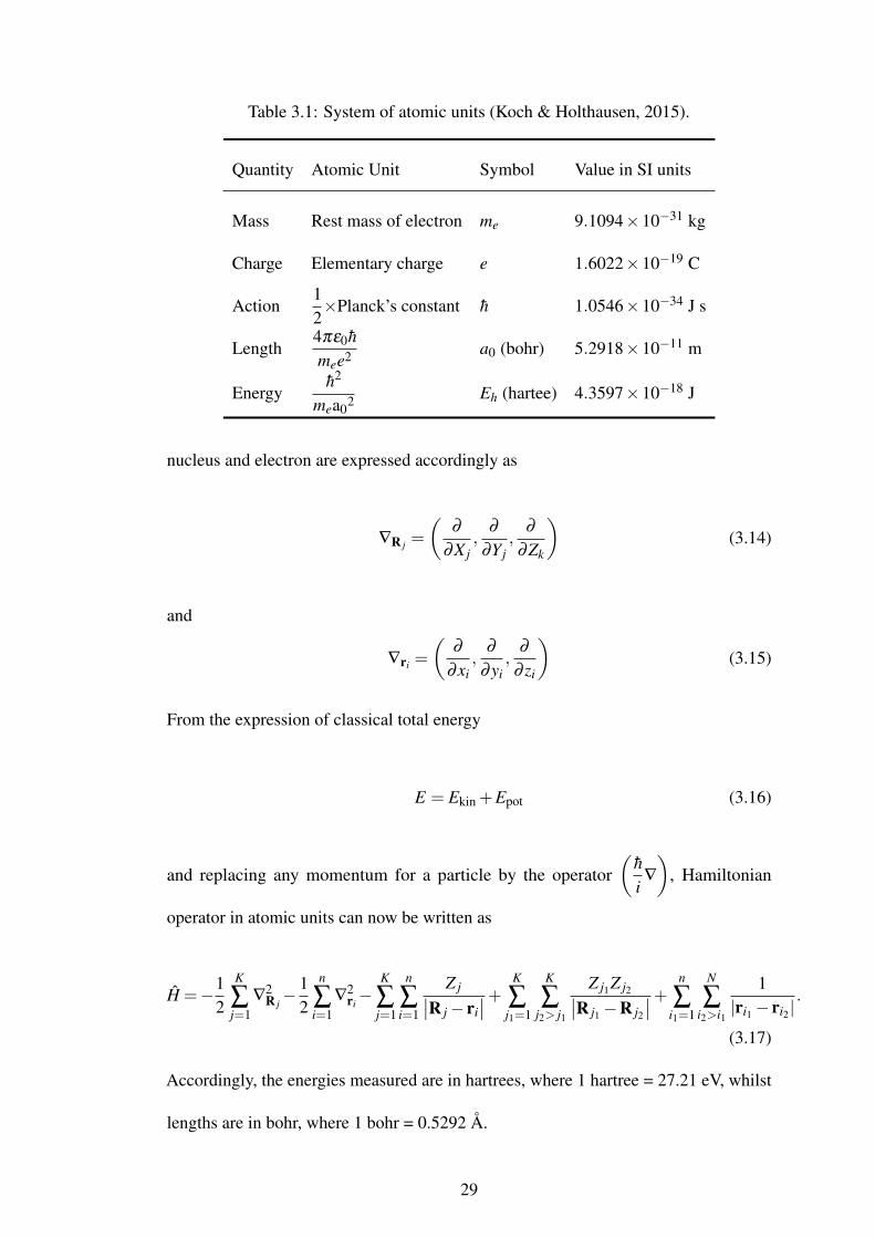
Table 3.1: System of atomic units (Koch & Holthausen, 2015).

Quantity Atomic Unit Symbol Value in SI units

Mass Rest mass of electron me 9.1094×10−31 kg

Charge Elementary charge e 1.6022×10−19 C

Action12×Planck’s constant h 1.0546×10−34 J s

Length4πε0hmee2 a0 (bohr) 5.2918×10−11 m

Energyh2

mea02 Eh (hartee) 4.3597×10−18 J

nucleus and electron are expressed accordingly as

∇R j =

(∂

∂X j,

∂

∂Y j,

∂

∂Zk

)(3.14)

and

∇ri =

(∂

∂xi,

∂

∂yi,

∂

∂ zi

)(3.15)

From the expression of classical total energy

E = Ekin +Epot (3.16)

and replacing any momentum for a particle by the operator(

hi∇

), Hamiltonian

operator in atomic units can now be written as

H =−12

K

∑j=1

∇2R j− 1

2

n

∑i=1

∇2ri−

K

∑j=1

n

∑i=1

Z j∣∣R j− ri∣∣+ K

∑j1=1

K

∑j2> j1

Z j1Z j2∣∣R j1−R j2

∣∣+ n

∑i1=1

N

∑i2>i1

1|ri1− ri2|

.

(3.17)

Accordingly, the energies measured are in hartrees, where 1 hartree = 27.21 eV, whilst

lengths are in bohr, where 1 bohr = 0.5292 Å.

29

3.4.2 The Born-Oppenheimer Approximation

In a real system, electric forces on nuclei and electrons are of the same magnitude,

and consequently both particles have comparable magnitudes of momenta. However,

the electrons move much faster than the nuclei due to significant mass different between

both types of particles. This leads to the fundamental idea of the Born-Oppenheimer

approximation (BO). One can picture that nuclei are held relatively fixed at their

locations, contributing zero kinetic energy but a merely constant potential energy to

total energy of the system, due to nucleus-nucleus repulsion. Whereas for the electrons,

they move instantaneously as the nuclei move (Springborg, 2000).

This approximation leads the Schödinger equation to consist only the electronic

part, whose solutions are the electronic wave function Ψelec and the electronic energy

Eelec,

HelecΨelec(r1,r2, ...,rn) = EelecΨelec(r1,r2, ...,rn) (3.18)

where the electronic Hamiltonian is given by

Helec =−12

n

∑i=1

∇2ri−

K

∑j=1

n

∑i=1

Z j∣∣R j− ri∣∣ + n

∑i1=1

n

∑i2>i1

1|ri1− ri2|

= T +VNe +Vee. (3.19)

It should be noted that VNe which denotes the attractive potential exerted by the nuclei

on the electrons, is termed as the external potential Vext in DFT. Also, total energy of

the system Etot is defined as the sum of Eelec and the constant nucleus-nucleus repulsion

term in Equation (3.13):

Etot = Eelec +K

∑j1=1

K

∑j2> j1

Z j1Z j2∣∣R j1−R j2

∣∣ = Eelec +Enuc. (3.20)

30

3.4.3 Electon Density and The Thomas-Fermi Model

As in Equation (3.18), the approximate solution Ψelec is an n-electon wavefunction

that depends on 4n variables, where for each electron it consists of three position-space

and one spin coordinates. In general, systems of interest contain a number of atoms and

each atom has more than an electron. Although the wavefunction allows one to obtain

all information necessary to study the system accurately, due to practical limitations,

the computation works are laborious.

To overcome this difficulty, one may suggest that computing the electron density

ρ(r) is more feasible than solving Schrödinger equation for the wavefunction. Con-

tradict to the wavefunction, this density is observable and can be measured through

experiment like X-ray diffraction (Koch & Holthausen, 2015). The ρ(r), also known as

the probability density, is defined as multiple integral over one of the spatial variables

and spin coordinates of n electrons

ρ(r) = n∫· · ·∫|Ψ(x1,x2, ...,xn)|2dx1dx2...dxn. (3.21)

As early as in late 1920s, Thomas and Fermi derived the first density functional

approach based on a quantum statistical model of electrons (Fermi, 1928; Thomas,

1927). In the Thomas-Fermi (TF) model, the energy of an atom is expressed as the sum

of kinetic energy, nucleus-electron attraction and electron-electron repulsion:

ETF [ρ(r)] = TTF [ρ(r)]+VNe [ρ(r)]+Vee [ρ(r)] (3.22)

31

Kinetic energy of this model is based on the uniform electron gas, where there is no

change in electron density, and it is expressed as

TTF [ρ(r)] =CTF

∫ρ

53 (r)dr, (3.23)

where CTF =3

10(3π2)

23 , which is computed from the jellium model. Considering the

nucleus-electron attraction as the electrostatic field (external potential) generated by K

nuclei,

Vext(r) =K

∑j=1

−Z j∣∣R j− r∣∣ , (3.24)

together with repulsive potentials expressed in classical way, Equation (3.22) becomes

ETF [ρ(r)] =CTF

∫ρ

53 (r)dr+

∫Vext(r)ρ(r)dr+

12

∫ ∫ρ(r)ρ(r′)|r− r′|

drdr′. (3.25)

Although TF model is only a rough approximation to the true kinetic energy and

it neglects the exchange and correlation effects completely, it describes the energy of

an atom purely in terms of ρ(r). In TF model, ρ(r) characterizes the ground-state of

the system, where the energy in Equation (3.25) is minimized under the constraint that

integrating over the density gives total number of electrons n:

n =∫

ρ(r)dr. (3.26)

3.4.4 The Hohenberg-Kohn Theorems

In previous section, Thomas and Fermi approximated that the energy of an atom

can be expressed in terms of electron density, in turn the resulting equations can be

32

solved easier than that of Schrödinger equation. However, it is not an approximation to

the "true" wavefunction-based approaches. Hohenberg and Kohn (1964) has shown that

it is possible to compute any ground-state property of a system using only the electron

density instead of full wavefunction.

Consider a n-electron system, where the electrons move in some external potential.

Here, the external potential can be referred to the electrostatic field due to the nuclei as in

Equation (3.24), as well as for the case where the system is exposed to the gravitational

field or external electrostatic. Similar to Equation (3.19), the total Hamiltonian operator

is thus

H =−12

n

∑i=1

∇2ri+

n

∑i=1

Vext(r)+V (r1,r2, ...,rn). (3.27)

Hohenberg and Kohn proved that electron density ρ(r) at the ground state of a given

system determines the external potential uniquely; there is no way for two different

external potentials, named Vext,1 and Vext,2, to produce the same density. This leads to

the first Hohenberg-Kohn theorem: once the ground-state electron density in position

space is known, any ground-state property of a given system, as a functional of ρ(r), is

uniquely defined.

At the ground state of a n-electron system, the total electronic energy Eelec, which

is a functional of ρ in position space, must be the minimum value of the expectation

value 〈Ψ|H|Ψ〉. Assume there are two different densities, ρ0 as the correct ground-

state density that is constructed from wavefunction Ψ while ρ ′ is a faulty density

obtained from wavefunction Ψ′. The energy Eelec(ρ′) obtained by minimizing the

expectation value 〈Ψ′|H|Ψ′〉 is never the ground-state energy of the system, and hence

33

the variational principle for the density functionals,

Eelec[ρ′(r)]≥ Eelec [ρ0(r)] (3.28)

leads to the second Hohenberg-Kohn theorem. This variational theorem proves that there

is no trial electron density ρ ′ can results in a lower ground-state energy than the true

ground-state energy. Therefore, in practice, one can use different ρ ′ in calculations and

eventually the approximated functional of ρ(r) can be obtained if the energy calculation

has converged.

3.4.5 The Kohn-Sham Approach

Although Hohenberg and Kohn (1964) proved the correctness of the Thomas-Fermi

model, they do not suggest a practical method to calculate ground-state properties

from the electron density. Later, Kohn and Sham (1965) have developed a method by

considering a system of non-interacting particles to overcome this problem. In this

method, the non-interacting reference system is assumed to have the same electron

density and energy as the real system.

To compute the kinetic energy for non-interacting fermions, Kohn and Sham (1965)

introduced a set of one-electron orbital, {ϕi}. Suppose that the electrons move in some

external potential Veff(r) and hence the one-electron Schrödinger equation (Guet, Hobza,

Spiegelman, & David, 2002) is given by

[−1

2~∇2 +Veff(r)

]ϕi = εiϕi. (3.29)

34

In terms of these one-electron orbitals, also known as KS orbitals, the electron density

of non-interacting reference system ρs(r) exactly equals to the ground-state density of

the real system with interacting particles:

ρs(r) =N

∑i=1

∑σ=↑,↓

|ϕi(r,σ)|2 = ρ0(r). (3.30)

In a real (interacting) and a fictitious (non-interacting) systems, the kinetic energies

in both system will be definitely different, even if both systems share the same electron

density. To take into account this difference, Kohn and Sham (1965) introduced a

universal functional

F [ρ(r)] = Ts [ρ(r)]+ J [ρ(r)]+Exc [ρ(r)] (3.31)

where Ts and J are respectively the kinetic energy and classical Coulomb repulsion

energy in the non-interacting reference system, while Exc is the exchange-correlation

energy:

Exc [ρ] = (T [ρ]−Ts [ρ])+(Vee [ρ]− J [ρ]). (3.32)

The first brackets in Equation (3.32) indicates the residual kinetic energy by taking

away the non-interacting contributions from the true kinetic energy, while the second

brackets indicates the non-classical electron-electron repulsion energy, which contains

all the effects of self-interaction correction, exchange and Coulomb correlation (Koch

& Holthausen, 2015).

For a real and interacting system, its total electronic energy can now be expressed

35

in terms of the separation described in Equation (3.31):

Eelec [ρ(r)] = Ts [ρ]+ J [ρ]+Exc [ρ]+VNe [ρ]

=−12

n

∑i=1〈ϕi∣∣∇2∣∣ϕi〉+

12

∫ ∫ρ(r)ρ(r′)|r− r′|

drdr′+Exc [ρ]+∫

Vext(r)ρ(r)dr.

(3.33)

Applying variational principle, Schrödinger equation for the real system is given as

(−1

2∇

2 +

[12

∫ρ(r′)|r− r′|

dr′+Vxc(r)+Vext(r)])

Ψ = EelecΨ, (3.34)

where the nucleus-electron interaction potential is defined by Equation (3.24). Compar-

ing this equation with the one-electron Schrödinger equation from the non-interacting

reference system, as in Equation (3.29), it arrives at

Veff =12

∫ρ(r′)|r− r′|

dr′+Vxc(r)−K

∑j=1

Z j∣∣R j− r∣∣ , (3.35)

where the exchange-correlation potential is given by

Vxc(r) =δExc [ρ]

δρ. (3.36)

Equations (3.29), (3.30) and (3.35) are known as the KS equations. It should be

noted that since the Coulomb term in Equation (3.35) indicates that the dependence of

Veff on the electron density as well as on the orbitals, these equations have to be solved

self-consistently. The KS equations are exact, and hence in principle KS method will

lead to the exact energy as well as the ground-state density. Although there is no exact

form for Vxc, as shown in Equation (3.35), there exists better and better approximations

36

for exchange-correlation energyExc and the corresponding potential Vxc in modern DFT.

In addition, there is no reference to the spin of electrons in the expression of

Veff. Thus, for a system with even number of electrons (closed-shell system), the KS

orbitals will occur in degenerate pairs where the spatial part is shared by a up-spin (α)

and a down-spin (β ) function. On the other hand, for a system with odd number of

electrons (open-shell system), the densities of both α-spin and β -spin electrons will

be different and hence, the total electron density is ρ(r) = ρα(r)+ρβ (r). In general,

DFT calculations will consider restricted KS (RKS) formalism for a closed-shell system

and unrestricted KS (UKS) formalism for an open-shell system. In principle, UKS

formalism is suitable for any kind of atom or molecule, closed- or open-shell system,

or a system with an arbitrary multiplicity (Koch & Holthausen, 2015), and hence it is

employed in DFT calculations of this work.

There is an iterative procedure to solve the KS equations. Firstly, an initial density

is chosen for a system, which is then used to construct an initial Hamiltonian. After

solving the eigenvalue problem, a set of KS orbitals, {ϕi}, will be obtained which is

used to derive a new electron density. Then, the new density is used to construct a new

Hamiltonian for the system. These processes are repeated until it achieves a certain

convergence criteria. The total energy and other properties of interest are recorded once

the convergence has been met.

3.4.6 Approximate Exchange-Correlation Functionals

According to the KS equations, the only remaining unknown term is the exchange-

correlation potential Vxc, which is a functional derivative of its corresponding energy

37

Exc. The solving of Schrödinger equation using the KS approach can only be done if

explicit approximations to the functional Exc are available. In other words, the accuracy

of chosen approximations to Exc defines the quality of density functional approach

(Koch & Holthausen, 2015).

The simplest and remarkable approximation for Exc [ρ(r)] is local-density approxi-

mation (LDA), which has been established originally with the KS theory (Kohn, 1999):

ELDAxc [ρ(r)] =

∫εxc [ρ(r)]ρ(r)dr, (3.37)

where εxc [ρ(r)] is the exchange-correlation energy per electron in a uniform electron

gas with density ρ(r). In a homogeneous electron gas, the system is electrically

neutral, consisting interacting electrons moving in a positively charged field. This

formalism assumes that a given material is composed of a number of extremely small

region, each with a constant electron density which contributes to the total exchange-

correlation energy. LDA works for systems with highly-homogeneous electron densities,

as well as realistic non-homogeneous systems. However, one of the drawbacks is its

overestimation of binding energies for molecules and solids.

Later, some high-level approximations have been developed to tackle this problem.

The strategy to do this is by including the gradient of the density instead of only the

information about the density ρ(r) at a particular point r. One of these high-level

approximations is known as generalized gradient approximation (GGA). For a spin-

polarized (unrestricted) system where the α and β spins are free to have different spatial

38

orbitals, this approximation is given by

EGGAxc

[ρα ,ρβ

]=∫

f (ρα ,ρβ ,∇ρα ,∇ρβ )dr, (3.38)

where f is some function of the spin densities and their gradients (Koch & Holthausen,

2015; Kohn, 1999; Levine, 2009). GGA is commonly used in studying molecular

system as in nanoparticles, and hence it is employed in this work.

3.4.7 Basis Sets

It is important to find a computationally efficient way in solving the KS equations.

The solutions of KS equations are the KS molecular orbitals, which yield the ground-

state density associated with the chosen Vxc. Almost all applications of KS DFT employ

the approach introduced by Roothaan (1951), known as LCAO expansion of the KS

molecular orbitals. In this scheme, it makes use of a set of L predefined basis function{ηµ

}(Koch & Holthausen, 2015). With the coefficients cµi, the KS orbitals are linearly

expanded as

ϕi =L

∑µ=1

cµiηµ . (3.39)

In the context of this work, the set{

ηµ

}is chosen to consist of so-called Gaussian-

type-orbitals (GTO). In Cartesian coordinates, GTO can be written as

ηGTO(x,y,z) = Axlxylyzlz exp

[−ζ r2] , (3.40)

where A is a normalisation constant, ζ is related to the width of the curve, and r2 gives

the curve a Gaussian shape. Also, the sum of lx, ly and lz determines the type of orbitals;

39

for instance, lx + ly + lz = 1 indicates a p-orbital (Jensen, 2013).

To conduct an in silico experiment, one should first choose a theoretical framework

in which interactions within the system can be sufficiently described. Typically the

interactions could be either in the form of an empirical forcefield, or described at the

quantum-mechanical level in the form of DFT. To summarize, this chapter has discussed

the theoretical background of the methods, i.e. the Gupta empirical forcefield and DFT,

used to describe the interactions within the clusters that are to be studied in this project.

40

CHAPTER 4

LOWEST-ENERGY CONFIGURATIONS OF RHODIUMCLUSTERS

In this chapter, the computational methodology and the procedure to obtain the

lowest energy states of the rhodium (Rh) clusters will be presented. The optimized

configurations for Rh clusters obtained, will be reported. Their atomic structures and

magnetism will also be discussed.

4.1 Computational Details

In the present study, the optimized configurations of Rh clusters are obtained in a

two-stage procedure. In the first stage, the novel global optimization algorithm BHGA

(which has been introduced in the previous chapter), is used to generate low-lying energy

Rh structures in the empirical PES of Gupta potential. These candidate structures are

then re-optimized using density functional theory (DFT) to obtain structures which are

representative of ground-state structures at the DFT level.

The parameters of many-body Gupta potential used to describe the interatomic

interactions in BHGA in the first-stage calculation (as given in Equation (3.1)) are

adopted from Cleri and Rosato (1993), see Table 4.1. In the beginning, 20 random

configurations are generated. Canonical Monte Carlo BH is performed on each of these

individuals for 5000 BH steps. Here, the local energy minimization algorithm employed

in BH is the limited-memory Broyden–Fletcher–Goldfarb–Shanno (BFGS), also known

as L-BFGS. Then, these individuals enter as first generation "parents" in the GA section

41

Table 4.1: Gupta potential parameters for Rh clusters, which are obtained from Cleriand Rosato (1993).

A (eV) ξ (eV) p q r0 (Å)

0.0629 1.6600 18.4500 1.8670 2.6890

of the optimization algorithm to breed "children" for the next generation. The fitness of

each of them is evaluated according to the definition Equation (3.5). Five individuals

with lowest fitness are discarded. In the next generation, 15 of the individuals retained

from the previous generation are randomly chosen and subjected to genetic operators

to generate five "children", replacing those discarded individuals, thus keeping the

population size at 20. The weighting of inversion, arithmetic mean, geometric mean,

N-point crossover, 2-point crossover and mutation operators are initialized respectively

as 5:1:1:5:5:5. In each generation, a "child" is optimized for 500 BH steps. The GA

optimization is continued for 500 generations. Lastly, 5000 BH steps are performed

on the 20 individuals separately again to ensure the lowest-possible energy value is

obtained from BHGA. The lowest-energy configuration is determined from the 20

individuals.

Electronic properties of the clusters, including their electronic distribution and

magnetic properties, are calculated using first-principles KS DFT. Calculations are

performed by using a DFT package called deMon2k (St-Amant & Salahub, 1990),

which employs linear combination of Gaussian-type orbital (LCGTO) approach to solve

the KS equations. The unrestricted KS (UKS) formalism is used in all calculations,

while the self-consistent field (SCF) energy converges at a threshold of 10−7 a.u..

Level-shift procedure that enlarges the gap between highest occupied molecular orbital

(HOMO) and lowest unoccupied molecular orbital (LUMO) (commonly known as

42

HOMO-LUMO gap) and mixing of charge density are applied to control and stabilize

the SCF. The choice of methodology can be crucial in DFT calculations and hence, it

is essential to carry out test calculations to determine the best methodology and basis

set for Rh clusters. In this thesis, total energy of a cluster is calculated within GGA by

using PBE exchange-correlation functional (Perdew, Burke, & Ernzerhof, 1996), which

is commonly used for clusters of transition metals. The energy value is evaluated after

self-consistency is achieved to ensure high accuracy and reliability of the results. Test

calculations are performed on Rh atom and its dimer (Rh2) with different basis sets, in

conjunction with GEN-A2 auxiliary function set. Eventually, it is found that the 17-

valence-electron basis for Los Alamos National Laboratory (LANL) quasi-relativistic

effective core potential (QECP), named QECP|LANL2DZ (Hay & Wadt, 1985), made

reasonably good agreement with previous experimental and theoretical studies. Results

of test calculations are presented and discussed in Section 4.2.

Initial atomic coordinates for each cluster are taken from the lowest-energy configu-

rations as optimized by BHGA in the previous stage. Given a tight-binding SCF starting

density, geometry optimization is applied to the initial structure without symmetry

constraint in a spin-unrestricted environment in Cartesian coordinates. Convergence

criterion for the optimization based on root mean square (RMS) forces is specified

at a threshold of 3× 10−4 a.u.. Level-shift procedure is also applied to stabilize the

SCF. The geometry optimization of the cluster has to be carried out in stages by going

through a series of level-shift tuning procedure. In the procedure, SCF convergence

of electron density is first achieved by a using a course level-shift value. When this

is achieved, a more refined SCF convergence is attained by tuning the level-shift to a

smaller value. This procedure is repeated until the most refined level-shift value beyond

43

Figure 4.1: Plot of relative energies for Rh5 (solid line with dots) and Rh17 (dotted linewith triangles) against spin multiplicity. For Rh5, the lowest-energy configuration hasa spin multiplicity of 8, whereas for Rh17, the lowest-energy configuration has a spinmultiplicity of 18.

which SCF can no longer converge. For example, the first optimization is done using

a shift-level of 0.1 a.u, where SCF convergence is achieved. Following that a second

optimization is restarted from previous electron density with a new shift-level of 0.05

a.u. If SCF converges with shift-level of 0.05 a.u., an even smaller value of 0.025 a.u.

will be used to restart a new round of SCF. If SCF fails to converge at 0.025 a.u, the

converged SCF using shift-level of 0.05 a.u. is the electron density that will be used.

Since magnetic properties are to be studied, the geometrical optimization of the

clusters, apart from the above consideration, must also include the effect arisen from

spin multiplicities, M. A spin multiplicity is defined by M = 2S+ 1, where S is the

total spin angular momentum. The geometry of a cluster is optimized one-by-one

using increasing values of M but with the same initial atomic coordinates. The largest

value of M at which the optimization series ends, Mmax, is determined as the point

44

where the energy difference relative to the lowest energy is equal or larger than 0.5

eV. For closed-shell clusters, the range of M is 1,3,5, · · · ,MMax, while for open-shell

ones, 2,4,6, · · · ,MMax. The value of M corresponds to the lowest energy within the

range of 1−MMax (for closed-shell systems) or 2−MMax (for open-shell systems)

is adopted as the value of M used for calculating magnetic properties in subsequent

calculations. To illustrate how the lowest-energy M value is determined, Figure 4.1 is

referred. Figure 4.1 illustrates the relative energy (∆E) versus M for a small cluster Rh5

and a relatively large cluster Rh17. Apparently, the point of lowest-energy in the former

case is located at M = 10, after which ∆E increases rapidly. On the other hand, Rh17

has a number of isomers in the range of 8≤M ≤ 16. It is therefore essential to explore a

larger M (in this case, M is explored up to 30) to assure that M = 18 indeed corresponds

to the minimum point. Based on the vast practical experience gained throughout this

thesis, it is found that ∆E will not drop to any new lower energy-minimum point after

experiencing an abrupt rise. Hence, in this thesis, a sufficiently wide range of M is

explored to identify the lowest energy-minimum point by using the abrupt increment in

the variation of the ∆E−M curves as a good indicator. This tactics is adopted for every

cluster regardless of its number of atoms. After locating the lowest-energy configuration,

frequency analysis, which will be discussed later in Chapter 5, is performed to make

sure the configuration is not in transition state (i.e. the configuration has to be free

from having any imaginary frequency). If the lowest-energy configuration is not a

minimum, the analysis is repeated to each of the configurations (with different values

of M which are sorted according to total energies in ascending order), until a true

minimum configurations is determined. The final optimized structure of a cluster is

then the non-transition-state lowest-possible-energy configuration obtained through this

45

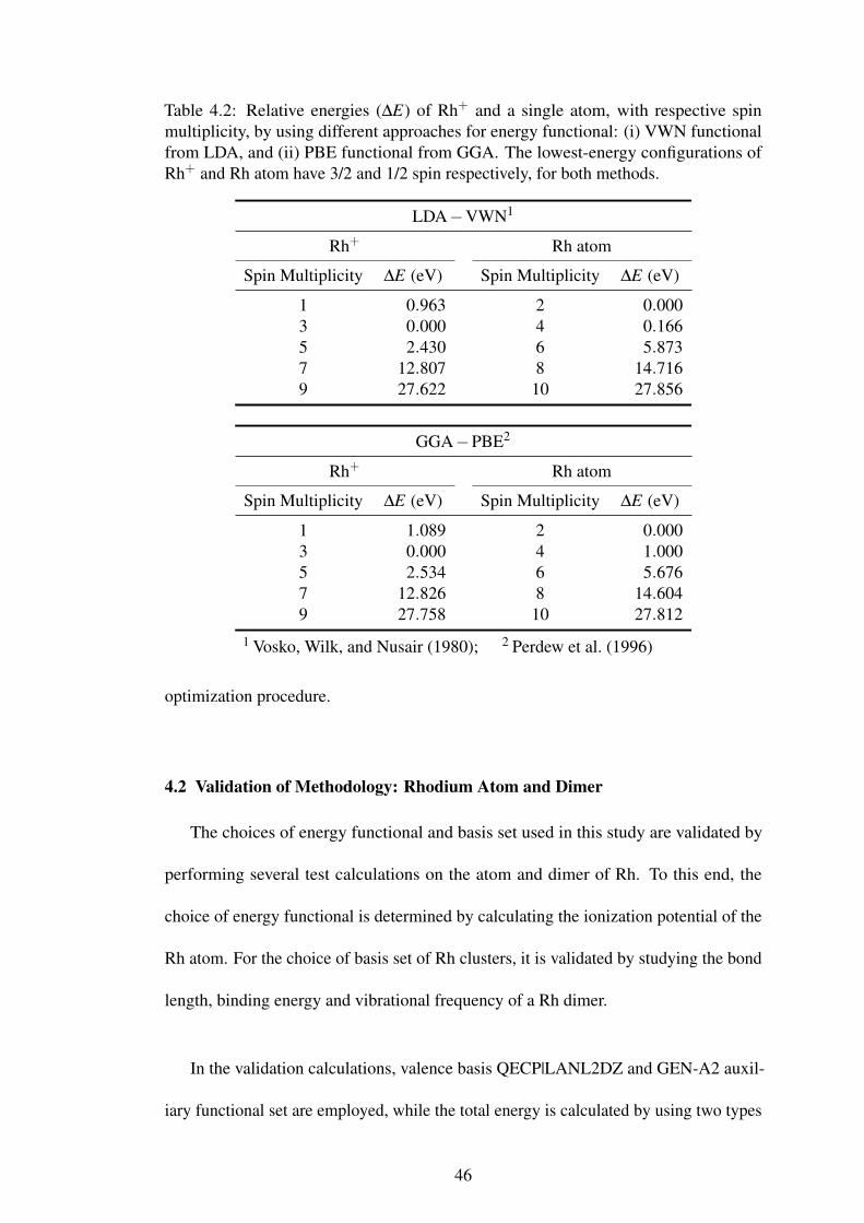
Table 4.2: Relative energies (∆E) of Rh+ and a single atom, with respective spinmultiplicity, by using different approaches for energy functional: (i) VWN functionalfrom LDA, and (ii) PBE functional from GGA. The lowest-energy configurations ofRh+ and Rh atom have 3/2 and 1/2 spin respectively, for both methods.

LDA−VWN1

Rh+ Rh atom

Spin Multiplicity ∆E (eV) Spin Multiplicity ∆E (eV)

1 0.963 2 0.0003 0.000 4 0.1665 2.430 6 5.8737 12.807 8 14.7169 27.622 10 27.856

GGA−PBE2

Rh+ Rh atom

Spin Multiplicity ∆E (eV) Spin Multiplicity ∆E (eV)

1 1.089 2 0.0003 0.000 4 1.0005 2.534 6 5.6767 12.826 8 14.6049 27.758 10 27.812

1 Vosko, Wilk, and Nusair (1980); 2 Perdew et al. (1996)

optimization procedure.

4.2 Validation of Methodology: Rhodium Atom and Dimer

The choices of energy functional and basis set used in this study are validated by

performing several test calculations on the atom and dimer of Rh. To this end, the

choice of energy functional is determined by calculating the ionization potential of the

Rh atom. For the choice of basis set of Rh clusters, it is validated by studying the bond

length, binding energy and vibrational frequency of a Rh dimer.

In the validation calculations, valence basis QECP|LANL2DZ and GEN-A2 auxil-

iary functional set are employed, while the total energy is calculated by using two types

46

of energy functional: (i) LDA approach by using VWN functional, and (ii) GGA ap-

proach by using PBE functional. To calculate the ionization potential, the lowest-energy

configurations of a Rh cation (Rh+) and a single Rh atom are determined. The relative

energies of these particles, where their spin multiplicities ranged from one to nine, are

presented in Table 4.2. The results from present calculations show that both energy

functions (i) and (ii) predicted the lowest-energy Rh atom has only an unpaired spin

(i.e. M = 2). This corresponds to the experimental results reported by Moore and Mack

(1952). In addition, the theoretical value of ionization potential, which is defined as

the energy difference between a cation and an atom, obtained from VWN and PBE are

8.66 eV and 8.35 eV respectively. As compared to the experimentally reported value of

7.46 eV (Moore & Mack, 1952), apparently the functional with GGA approach made a

better agreement and therefore, the exchange-correlation functional of PBE is employed

to calculate the total energy of Rh clusters throughout this work.

Next, the most suitable basis set is determined, as follows. In conjunction with

PBE functional and GEN-A2 auxiliary function set, test calculations are performed

by relaxing the Rh dimer (Rh2) with various types of basis set, including the double

ζ polarization basis sets (DZVP), effective core potential (ECP), model core poten-

tial (MCP), quasi-relativistic effective core potential (QECP) and relativistic model

core potential (RMCP). All basis sets for Rh available in deMon2k package are respec-

tively developed by Stuttgart/Dresden (SD), Lovallo and Klobukowski (2002, 2003)

(LK) and Los Alamos National Laboratory (LANL) (Feller, 1996; Schuchardt et al.,

2007). Table 4.3 reports the bond length, binding energy and vibrational frequency

obtained after optimizing Rh2 for each of these basis sets. Also, the results reported

by previous experimental studies and theoretical calculations with LCAO approach are

47

Table 4.3: Bond lengths (d), binding energies (Eb) and vibrational frequencies (ω0)of ground-state Rh2 with different types of basis sets. In present work and theoreti-cal references, each of these configurations have the same magnetic moment of 2.0µB/atom.

Basis Setd

(Å)Eb

(eV/atom)ω0

(cm−1)

Presentwork

DZVP-GGA 2.318 1.500 282.20ECP|SD 2.292 1.429 288.10ECP17|SD 2.292 1.429 288.10MCP15|LK 2.270 1.638 299.00QECP|LANL2DZ 2.291 1.767 295.10QECP|SD 2.222 1.907 347.40QECP17|SD 2.222 1.907 347.40RMCP15|LK 2.248 2.189 305.20

Theoreticalstudies

2.2602.3312.3402.2602.2702.2792.260

1.510–

1.880–

0.8001.4391.480

–282.00

–––

309.04–

Ref. [1]Ref. [2]Ref. [3]Ref. [4]Ref. [5]Ref. [6]Ref. [7]

Experimentalstudies

2.280–

1.460±0.1100.700±0.150

267.00283.90±1.80

Ref. [8]Ref. [9]

1 Nayak et al. (1997); 2 Chien, Blaisten-Barojas, and Pederson (1998);3 Reddy, Nayak, Khanna, Rao, and Jena (1999); 4 Y. Sun, Fournier, and Zhang (2009);5 Beltrán et al. (2013); 6 Soltani and Boudjahem (2014);7 Hang et al. (2015); 8 Gingerich and Cocke (1972) and Cocke and Gingerich (1974);9 H. Wang et al. (1997)

also presented in Table 4.3 for comparison.

The total magnetic moment of lowest-energy Rh2 obtained from present calculations,

regardless of basis set employed, has a total magnetic moment of 4 µB. Although the

spin multiplicity of a Rh2 is yet to be determined experimentally, all theoretical studies

predicted a quintet spin state (M = 5)for the dimer and hence, present results make

excellent agreement with these works.

Before reporting present results, previous works are reviewed in short. In an early

48

experimental studies, Gingerich and Cocke (1972) performed a Knudsen effusion

experiment and measured the chemical equilibrium of Rh2 in its gaseous state. This

study estimated that the dimer has a vibrational frequency of 267 cm−1 and the two

atoms are separated by 2.28 Å. Besides, they have also suggested the binding energy

of the dimer, is ranged from 1.35 eV to 1.57 eV (Cocke & Gingerich, 1974). Later,

H. Wang et al. (1997) performed the spectroscopy of mass-selected Rh dimers in argon

matrices and reported a value of 0.700 eV with discrepancies of 0.15 eV for binding

energy, whilst the frequency is given by (283.90±1.80) cm−1. At the same time, the

calculated bond lengths are also agreed with theoretical values predicted previously. On

the other hand, theoretical studies which employed the LCAO approach in solving the

KS equations, generally obtained bond length that agreed with the experimental bond

length. While for the binding energy, most of the studies reported values that are in

the range of energies suggested by Cocke and Gingerich (1974) except Beltrán et al.

(2013) who used a larger TZVP basis set, is the only study made excellent agreement

with H. Wang et al. (1997).

As shown in Table 4.3, the values of bond length obtained using different basis

sets are all in excellent agreement with the experimental bond length, as well as those

reported theoretically. Thus, bond length is not a good criteria in choosing basis

sets. Steps to determine the most suitable basis set for Rh clusters are explained as

follows. Firstly, QECP|SD, QECP17|SD and RMCP15|LK have been eliminated from

consideration as the values of binding energies and vibrational frequencies obtained

using these basis sets are overestimated from the reference values. As mentioned

previously, the level-shift applied in DFT calculations enlarges the HOMO-LUMO gap

of a cluster and hence, it should be kept at minimum so that it will not affect the accuracy

49

Figure 4.2: Optimized structures of the RhN (3≤ N ≤ 5) clusters via DFT calculations.

of results obtained. Taking into account the shifting parameter, only MCP15|LK and

QECP|LANL2DZ allowed the SCF to be converged at a shift value as low as 0.01 a.u..

Lastly, the QECP|LANL2DZ which resulted in a closer value of vibrational frequency

to those from references, is chosen for all of the following calculations.

4.3 Optimized Configurations of Rhodium Clusters

By following the first stage process as mentioned in the methodology as described in

the previous section, optimized configurations of Rh clusters up to 38 atoms in the PES

of Gupta potential are obtained. A full list of these configurations can be found in the

Appendix A. These configurations will be used as initial structures for DFT optimization

in the second stage of the calculation procedure. Due to the expensive computational

cost, first-principles optimization will focus only on clusters up to 23 atoms, and threes

selective cluster sizes, namely, 26, 30 and 38. In the following, the optimized structures,

along with their associated magnetic moment and symmetries, obtained in present work

are presented, discussed and compared in a systematic order. More technical details of

point symmetry and symmetry order pertinent the geometrical description of clusters

will be discussed again in Section 5.4 in Chapter 5.The discussions will start from Rh3

since the Rh atom and its dimer have been discussed in previous session.

50

Table 4.4: Comparison of the present results on optimized configurations of Rh3 withprevious calculations.

Symmetry Description Total magnetic moment (µB)

Present C2v Isosceles triangle 5

Ref. [1] Equilateral triangle 3Ref. [2] C2v Isosceles triangle 5Ref. [3] C2v

D3h

Isosceles triangleEquilateral triangle

53

Ref. [4] Triangle 3Ref. [5] Equilateral triangle 3Ref. [6] C2v Isosceles triangle 5Ref. [7] D3h Equilateral triangle 3Ref. [8] D3h Equilateral triangle 31 Nayak et al. (1997) 2 Chien et al. (1998)3 Reddy et al. (1999) 4 Da Silva, Piotrowski, and Aguilera-Granja (2012)5 Mokkath and Pastor (2012) 6 Beltrán et al. (2013)7 Soltani and Boudjahem (2014) 8 Hang et al. (2015)

Table 4.4 compared the optimized configuration of Rh3 from present calculation

against that from the literature. The lowest configurations reported by Da Silva et

al. (2012) and Mokkath and Pastor (2012), which have employed pseudopotential

approximation, are triangles with total magnetic moment of 3 µB. This result is

consistent with those calculations using LCAO approach which obtained a quintet

equilateral-triangular Rh3 (Hang et al., 2015; Nayak et al., 1997; Soltani & Boudjahem,

2014). Also, Reddy et al. (1999) claimed that the energy difference between an isosceles

and an equilateral triangle of Rh3 is negligible, hence, both structures are in a degenerate

state. Present calculation which obtains an isosceles triangular with spin multiplicity of

6, as shown in Figure 4.2, makes a good agreement with Chien et al. (1998) and Beltrán

et al. (2013).

Rh4 is the smallest cluster with three-dimensional motif. From the geometry

optimization, a couple of isomers is obtained at the lowest-energy level. The first

51

Table 4.5: Comparison of the present results on optimized configurations of Rh4 withprevious calculations. In present work, there are two isomers found at lowest-energylevel: (i) non-magnetic tetrahedron, and (ii) septet rhombus.

Symmetry Description Total magnetic moment (µB)

Present TdD2d

TetrahedronBent rhombus

06

Ref. [1 ] SquareTetrahedron

40

Ref. [2] Td Tetrahedron 0Ref. [3] Tetrahedron 0Ref. [4] Bent rhombus 6Ref. [5] Tetrahedron 0Ref. [6] Tetrahedron 0Ref. [7] C1 Bent rhombus 6Ref. [8] D2d Bent rhombus 6Ref. [9] Td

C1

TetrahedronTetrahedron

06

1 Nayak et al. (1997) 2 Chien et al. (1998) 3 Reddy et al. (1999)4 Bae, Osanai, Kumar, and Kawazoe (2004) 5 Da Silva et al. (2012)6 Mokkath and Pastor (2012) 7 Beltrán et al. (2013)8 Soltani and Boudjahem (2014) 9 Hang et al. (2015)

isomer is found to be a non-magnetic tetrahedron with sides 2.49 Å, while the second

isomer, whose energy is 5 meV higher than the first isomer, is a bent rhombus with a

total magnetic moment of 6 µB. The isomers of Rh4 are named as Rh4(a) and Rh4(b)

respectively in Figure 4.2. This results in general match well with those reported

previously, as summarized in Table 4.5. Despite of the proposition that a structure with

high symmetry promotes larger magnetic moment (Dunlap, 1990; T.-W. Yen & Lai,

2016), it does not happen in this case. In the presence case, it is observed that highly

symmetric tetrahedron is non-magnetic. Conversely, a highly distorted (low symmetric)

structures obtained by Beltrán et al. (2013) and Hang et al. (2015) have relatively high

magnetic moment at 6 µB.

Most of the previous studies reported the ground-state structure of Rh5 as a quintet

52

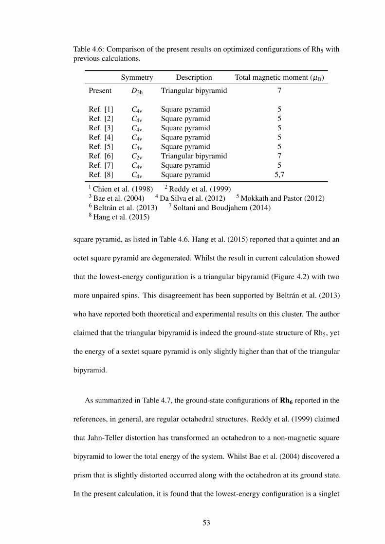
Table 4.6: Comparison of the present results on optimized configurations of Rh5 withprevious calculations.

Symmetry Description Total magnetic moment (µB)

Present D3h Triangular bipyramid 7

Ref. [1] C4v Square pyramid 5Ref. [2] C4v Square pyramid 5Ref. [3] C4v Square pyramid 5Ref. [4] C4v Square pyramid 5Ref. [5] C4v Square pyramid 5Ref. [6] C2v Triangular bipyramid 7Ref. [7] C4v Square pyramid 5Ref. [8] C4v Square pyramid 5,71 Chien et al. (1998) 2 Reddy et al. (1999)3 Bae et al. (2004) 4 Da Silva et al. (2012) 5 Mokkath and Pastor (2012)6 Beltrán et al. (2013) 7 Soltani and Boudjahem (2014)8 Hang et al. (2015)

square pyramid, as listed in Table 4.6. Hang et al. (2015) reported that a quintet and an

octet square pyramid are degenerated. Whilst the result in current calculation showed

that the lowest-energy configuration is a triangular bipyramid (Figure 4.2) with two

more unpaired spins. This disagreement has been supported by Beltrán et al. (2013)

who have reported both theoretical and experimental results on this cluster. The author

claimed that the triangular bipyramid is indeed the ground-state structure of Rh5, yet

the energy of a sextet square pyramid is only slightly higher than that of the triangular

bipyramid.

As summarized in Table 4.7, the ground-state configurations of Rh6 reported in the

references, in general, are regular octahedral structures. Reddy et al. (1999) claimed

that Jahn-Teller distortion has transformed an octahedron to a non-magnetic square

bipyramid to lower the total energy of the system. Whilst Bae et al. (2004) discovered a

prism that is slightly distorted occurred along with the octahedron at its ground state.

In the present calculation, it is found that the lowest-energy configuration is a singlet

53

Figure 4.3: Optimized structures of the RhN (6≤ N ≤ 8) clusters via DFT calculations.In present work, a non-magnetic and a septet octahedral structures are found at thelowest-energy level.

Table 4.7: Comparison of the present results on optimized configurations of Rh6 withprevious calculations.

Symmetry Description Total magnetic moment (µB)

Present OhOh

OctahedronOctahedron

06

Ref. [1] Oh Octahedron 6Ref. [2] D4h Square bipyramid 0Ref. [3] Octahedron

Prism66

Ref. [4] Octahedron 6Ref. [5] Octahedron 6Ref. [6] Oh Octahedron 6Ref. [7] Oh Octahedron 6Ref. [8] Oh Octahedron 61 Chien et al. (1998) 2 Reddy et al. (1999) 3 Bae et al. (2004)4 Da Silva et al. (2012) 5 Mokkath and Pastor (2012) 6 Beltrán et al.(2013) 7 Soltani and Boudjahem (2014) 8 Hang et al. (2015)

octahedron (Figure 4.3) with bond length of 2.55 Å. The result of the present calculation

also found that there is another competing isomer sitting at the same ground state. This

isomer is an magnetic octahedron with sides of 2.58 Å. This result shows that geometry

of a cluster will indeed affect its magnetism. Since the energy of a septuplet octahedron

relative to the singlet octahedron is only 27 meV, they are considered to be degenerated.

The comparison of the results on lowest-energy configuration of Rh7 are summa-

54

Table 4.8: Comparison of the present results on optimized configurations of Rh7 withprevious calculations.

Symmetry Description Total magnetic moment (µB)

Present D5h Pentagonal bipyramid 13

Ref. [1] Pentagonal bipyramid 9Ref. [2] Square capped prism 11Ref. [3] Square capped prism 11Ref. [4] Pentagonal bipyramid 13Ref. [5] C1 Pentagonal bipyramid 13Ref. [6] C2v Square capped prism 9Ref. [7] C1

C2v

Capped octahedronPentagonal bipyramid

79

1 Reddy et al. (1999) 2 Bae et al. (2004) 3 Da Silva et al. (2012)4 Mokkath and Pastor (2012) 5 Beltrán et al. (2013)6 Soltani and Boudjahem (2014) 7 Hang et al. (2015)

rized in Table 4.8. The present calculation resulted in a pentagonal bipyramid Figure 4.3

with a total magnetic moment of 13 µB, which makes a good agreement with the

configuration reported by Mokkath and Pastor (2012). It is also interesting to find

that distortion of the atomic structure lowered the magnetism of the cluster. A regular

pentagonal bipyramid is supposed to have a D5h symmetry, as obtained from present

calculation. However, the bipyramids predicted by Hang et al. (2015); Reddy et al.

(1999) are less symmetric structures (C2v has a lower symmetry order). In other words,

these structures are distorted to some extent, where the symmetry elements are broken,

and these distortions has apparently reduced the magnetic moments of Rh7. An excep-

tion is found in Beltrán et al. (2013), which obtained a high magnetic moment with

pentagonal pyramid with C1 symmetry (lowest order of symmetry). In a recent study,

Hang et al. (2015) has suggested that a capped octahedron and a pentagonal bipyramid,

both are distorted, compete at the ground state.

While for Rh8 clusters, apparently, it is a competition between a cubic structure and

55

Table 4.9: Comparison of the present results on optimized configurations of Rh8 withprevious calculations.

Symmetry Description Total magnetic moment (µB)

Present D2d Bicapped octahedron 12

Ref. [1] Cube 12Ref. [2] Cube 12Ref. [3] Cube 12Ref. [4] C2v Bicapped octahedron 12Ref. [5] Cube 12Ref. [6] Oh Cube 121 Bae et al. (2004) 2 Da Silva et al. (2012) 3 Mokkath and Pastor (2012)4 Beltrán et al. (2013) 5 Soltani and Boudjahem (2014)6 Hang et al. (2015)

a bicapped octahedron, as shown in Table 4.9. Although many of the previous works

have reported that the eight atoms form a simple cube at the ground state, the present

calculation obtains an octahedron capped by two additional atoms, with a symmetry

group of D2d, as shown in Figure 4.3. This result is consistent with the results published

by Beltrán et al. (2013), yet the symmetry of their structure is only C2v (which is a lower

symmetry than D2d), indicating it is a distorted bicapped octahedron. It is interesting to

note that regardless of the geometry of Rh8, the lowest-energy configurations published

in the literature, as well as that obtained in this work, have a non-varying total magnetic

moment of 12 µB.

The optimized configuration of Rh9 obtained from present calculation is compared

with those reported previously in Table 4.10. Soltani and Boudjahem (2014) estimated a

capped cubic structure as the ground-state configuration is favoured over those reported

by Bae et al. (2004) and Da Silva et al. (2012) because the magnetic moment of the

cluster obtained in the former falls in the range of discrepancies of experimental results.

Hang et al. (2015) claimed that the ground states comprised of two isomers with

56

Figure 4.4: Optimized structures of the RhN (9≤N ≤ 13) clusters via DFT calculations.

Table 4.10: Comparison of the present results on optimized configurations of Rh9 withprevious calculations. Experimental result is as given in Cox et al. (1993) and Cox et al.(1994).

Symmetry Description Total magnetic moment (µB)

Present D3h Double trigonal antiprism 1

Ref. [1] Capped cube 13Ref. [2] Capped cube 13Ref. [3] C1 Capped square antiprism 17Ref. [4] C4v Capped cube 9Ref. [5] C1 Tricapped trigonal prism 11,15Experiment 7.2±1.81 Bae et al. (2004) 2 Da Silva et al. (2012) 3 Beltrán et al. (2013)4 Soltani and Boudjahem (2014) 5 Hang et al. (2015)

tricapped trigonnal prism structure, where their lowest energy level are occupied by

a different spin configuration. Meanwhile, the next higher energy isomer is a capped

square antiprism with a total magnetic moment of 17 µB, which, in turn, is reported as

the ground-state structure by Beltrán et al. (2013). Nonetheless, results from present

calculations do not agree with that from the literature. The initial configuration for

57

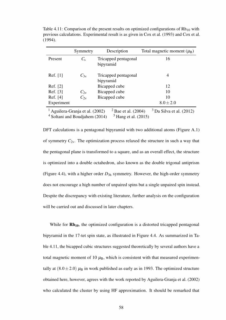
Table 4.11: Comparison of the present results on optimized configurations of Rh10 withprevious calculations. Experimental result is as given in Cox et al. (1993) and Cox et al.(1994).

Symmetry Description Total magnetic moment (µB)

Present Cs Tricapped pentagonal 16bipyramid

Ref. [1] C3v Tricapped pentagonal 4bipyramid

Ref. [2] Bicapped cube 12Ref. [3] C2v Bicapped cube 10Ref. [4] C2v Bicapped cube 10Experiment 8.0±2.01 Aguilera-Granja et al. (2002) 2 Bae et al. (2004) 3 Da Silva et al. (2012)4 Soltani and Boudjahem (2014) 5 Hang et al. (2015)

DFT calculations is a pentagonal bipyramid with two additional atoms (Figure A.1)

of symmetry C2v. The optimization process relaxed the structure in such a way that

the pentagonal plane is transformed to a square, and as an overall effect, the structure

is optimized into a double octahedron, also known as the double trigonal antiprism

(Figure 4.4), with a higher order D3h symmetry. However, the high-order symmetry

does not encourage a high number of unpaired spins but a single unpaired spin instead.

Despite the discrepancy with existing literature, further analysis on the configuration

will be carried out and discussed in later chapters.

While for Rh10, the optimized configuration is a distorted tricapped pentagonal

bipyramid in the 17-tet spin state, as illustrated in Figure 4.4. As summarized in Ta-

ble 4.11, the bicapped cubic structures suggested theoretically by several authors have a

total magnetic moment of 10 µB, which is consistent with that measured experimen-

tally at (8.0±2.0) µB in work published as early as in 1993. The optimized structure

obtained here, however, agrees with the work reported by Aguilera-Granja et al. (2002)

who calculated the cluster by using HF approximation. It should be remarked that

58

although the structure obtained by Aguilera-Granja et al. (2002) has a higher order of

symmetry, the distorted structure obtained from this work promotes the cluster to a

higher spin state.

Unlike small clusters that have unique geometries, the structures of clusters with

more than 10 atoms are generally extensions of the small clusters. As far as Rh11 is

concerned, several capping patterns have been suggested theoretically. According to

Aguilera-Granja et al. (2002), four atoms are capped to a pentagonal bipyramid and

produced a net spin of 13.77 µB. The capping of a single atom to different surface

of bicapped cubic structure is also found to arise in different magnetic moment. For

instance, Hang et al. (2015) found that three isomers compete at the lowest energy

level: (i) two structures which the atom capped on the surface of triangular prism are in

doublet and dectet spin state, and (ii) a structure which the atom capped on the surface

of cube is in octet spin state. Even with the similar structure as (i), the structure obtained

by Soltani and Boudjahem (2014) has total magnetic moment of 13 µB. From present

calculation, it is shown that the optimized configuration of Rh11 is formed by capping

two atoms to the central plane of double octahedron, as in optimized Rh9 (Figure 4.4).

While a structure with sextet spin state is obtained from this work, Bae et al. (2005)

obtained the similar structure, named as fused pentagonal pyramids, with a higher spin

at 16-tet. As an overall, most of the theoretical results including present calculation

made reasonable agreement with the experimental value of magnetic moment, which is

(8.8±2.2) µB (Cox et al., 1994).

From present calculations, Rh12 is the first cluster that consists of a central atom and

this leads to an icosahedral growth. Consistent with Reddy et al. (1999), the optimized

59

Table 4.12: Comparison of the present results on optimized configurations of Rh13 withprevious calculations. Experimental result is as given in Cox et al. (1993) and Cox et al.(1994).

Symmetry Description Total magnetic moment (µB)

Present D2h Icosahedron 15

Ref. [1] Icosahedron 15Ref. [2] Ih Icosahedron 16.38Ref. [3] Icosahedron 21Ref. [4] Cage 17Ref. [5] Biplanar 17Ref. [6] Capped double cube 9Ref. [7] Capped double cube 9Ref. [8] Capped double cube 9Ref. [9] Capped double cube 1Ref. [10] Capped double cube 9Ref. [11] Capped double cube 9Ref. [12] Capped double cube 9Ref. [13] Cs Capped double cube 9Ref. [14] C1 Biplanar 11Ref. [15] C1 Capped double cube 1Experiment 6.24±1.691 Reddy et al. (1999) 2 Aguilera-Granja et al. (2002) 3 Kumar and Kawazoe(2003) 4 Bae et al. (2004) 5 Chang and Chou (2004) 6 Bae et al. (2005)7 L.-L. Wang and Johnson (2007) 8 Aguilera-Granja, García-Fuente, and Vega(2008) 9 Y. Sun et al. (2009) 10 Piotrowski, Piquini, and Da Silva (2010)11 Da Silva et al. (2012) 12 Mokkath and Pastor (2012) 13 Chou, Hsing, Wei,Cheng, and Chang (2013) 14 Calaminici, Janetzko, Koster, Mejia-Olvera, andZuniga-Gutierrez (2007) 15 Hang et al. (2015)

configuration is an icosahedron with a missing cap atom with total magnetic moment of

18 µB, as illustrated in Figure 4.4. Although Aguilera-Granja et al. (2002) reported the

same geometry and symmetry (C5v), the cluster is only slightly magnetic with an average

value of 0.24 µB/atom. Along with the bilayer structure reported by Bae et al. (2004),

these results do not agree with the experimental value at (0.59±0.12) µB/atom (Cox

et al., 1994). However, in recent studies, double cube is claimed to be the ground-state

structure as its magnetic moment is close to the one reported experimentally (Da Silva

et al., 2012; Hang et al., 2015; Soltani & Boudjahem, 2014).

60

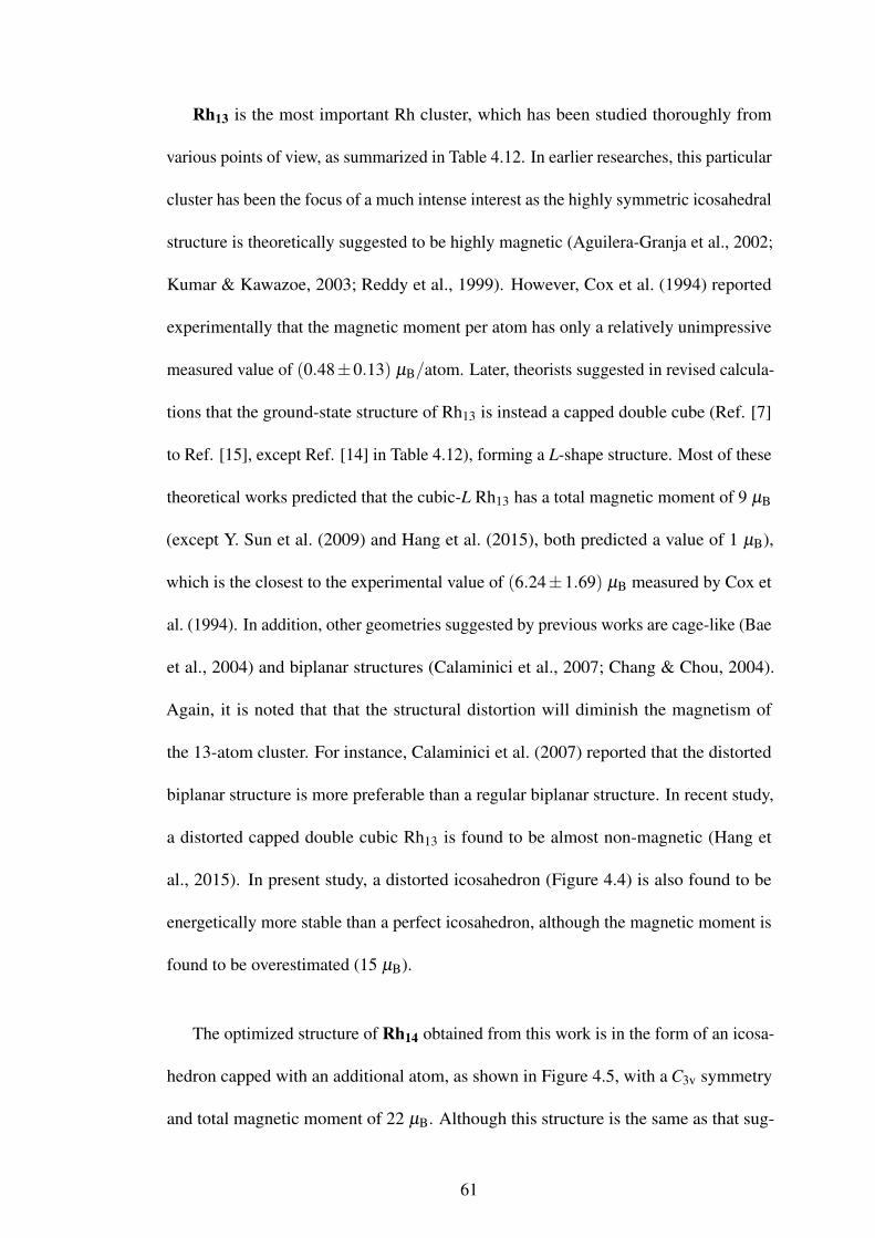
Rh13 is the most important Rh cluster, which has been studied thoroughly from

various points of view, as summarized in Table 4.12. In earlier researches, this particular

cluster has been the focus of a much intense interest as the highly symmetric icosahedral

structure is theoretically suggested to be highly magnetic (Aguilera-Granja et al., 2002;

Kumar & Kawazoe, 2003; Reddy et al., 1999). However, Cox et al. (1994) reported

experimentally that the magnetic moment per atom has only a relatively unimpressive

measured value of (0.48±0.13) µB/atom. Later, theorists suggested in revised calcula-

tions that the ground-state structure of Rh13 is instead a capped double cube (Ref. [7]

to Ref. [15], except Ref. [14] in Table 4.12), forming a L-shape structure. Most of these

theoretical works predicted that the cubic-L Rh13 has a total magnetic moment of 9 µB

(except Y. Sun et al. (2009) and Hang et al. (2015), both predicted a value of 1 µB),

which is the closest to the experimental value of (6.24±1.69) µB measured by Cox et

al. (1994). In addition, other geometries suggested by previous works are cage-like (Bae

et al., 2004) and biplanar structures (Calaminici et al., 2007; Chang & Chou, 2004).

Again, it is noted that that the structural distortion will diminish the magnetism of

the 13-atom cluster. For instance, Calaminici et al. (2007) reported that the distorted

biplanar structure is more preferable than a regular biplanar structure. In recent study,

a distorted capped double cubic Rh13 is found to be almost non-magnetic (Hang et

al., 2015). In present study, a distorted icosahedron (Figure 4.4) is also found to be

energetically more stable than a perfect icosahedron, although the magnetic moment is

found to be overestimated (15 µB).

The optimized structure of Rh14 obtained from this work is in the form of an icosa-

hedron capped with an additional atom, as shown in Figure 4.5, with a C3v symmetry

and total magnetic moment of 22 µB. Although this structure is the same as that sug-

61

Figure 4.5: Optimized structures of the RhN (14≤ N ≤ 19) clusters via DFT calcula-tions.

gested by Aguilera-Granja et al. (2002) (obtained using HF approximation), the total

magnetic moment of the cluster is much lower at 5.46 µB, which is in good agreement

with the experimental value of (7.00±1.68) µB (Cox et al., 1994). In addition, another

ground-state structure of Rh14 that has been suggested is a bicapped double cube, where

both additional atoms are capped on a specific side of the double cube (Bae et al., 2005;

Da Silva et al., 2012).

The following cluster, Rh15, is found experimentally to have a magnetic moment in

the range from 9.3 µB to 12µB. Hexagonal structure as suggested by Bae et al. (2004)

had a slightly overestimated magnetic moment of 19µB. In the present calculation, the

62

same value of magnetic moment as that of Bae et al. (2004) is also obtained, with the

optimized structure found to be a bicapped icosahedron (Figure 4.5). Besides, capping

of cubic structure has been reported by Bae et al. (2005) and Da Silva et al. (2012),

where the values of total magnetic moment are 7 µB and 9 µB respectively.

As for the Rh16, the optimized configuration obtained from present work is an

icosahedron capped with three atoms, with total magnetic moment of 14 µB. This

structure is comparable to that obtained by Aguilera-Granja et al. (2002), but the latter

has only magnetic moment of 6.24 µB. These two theoretical values made reasonable

discrepancies with respect to the experimental value of (10.24±1.60) µB (Cox et al.,

1994).

In the previous three capped structures, the atoms are capped in such a way to form

another plane. For the Rh17, the forth atom is not added on the growing plane but near

to the plane of icosahedron, as shown in Figure 4.5. This configuration has a magnetic

moment of 17 µB, which is overestimated as compared to that obtained from experiment

at (6.63±2.04) µB (Cox et al., 1994). On the other hand, the cubic structure of Rh17

suggested by Bae et al. (2005) was nearly non-magnetic.

While for the following cluster, Rh18, the optimized configuration obtained from

this study is a double icosahedron with a missing atom, as illustrated in Figure 4.5.

The calculated magnetic moment of this structure from this work is overestimated (20

µB) as compared to the experimental value of (4.20±1.44) µB. Even though Aguilera-

Granja et al. (2002) claimed that the lowest-energy structure is the one similar to that

obtained from this work, their magnetic moment obtained is 5.58 µB, which makes

63

Figure 4.6: Optimized structures of the RhN (20≤ N ≤ 23) clusters via DFT calcula-tions.

good agreement with experimental value.

As far as icosahedral growth is concerned, Rh19 is another important cluster which

acts as the second checkpoint of the growth pattern. Unlike a regular double icosahedron

(D5h) obtained by Aguilera-Granja et al. (2002) with 11 µB, present calculation shows

that the optimized configuration is a slightly distorted double icosahedron with a D2

symmetry (Figure 4.5) at the doublet spin state. This value of magnetic moment is in

good agreement with other theoretical works with capped cubic structure as the ground-

state structure (Bae et al., 2005; Mokkath & Pastor, 2012). In general, DFT calculations

yield the configurations with underestimated magnetic moment as compared to the

experimental value of (11.59±1.20) µB.

64

Table 4.13: Comparison of the present results on magnetism of optimized RhN (20≤N ≤ 23) with previous calculations. Among these clusters, only Rh22 have two isomerswith similar structure at the lowest-energy level, which respectively located at tripletand quintet spin state. Experimental result is as given in Cox et al. (1993) and Cox et al.(1994).

NTotal magnetic moment (µB)

Present Ref. [1] Ref. [2] Ref. [3] Experiment

20 4.00 1.60 – – 3.20±3.2021 1.00 1.60 – – 3.99±3.36

222.00

0.44 – – 5.94±3.084.00

23 5.00 0.69 8.97 8.97 2.99±2.991 Aguilera-Granja et al. (2002) 2 Bae et al. (2005)3 Aguilera-Granja et al. (2008)

Based on the experimental work done by Cox et al. (1994), the magnetism of clusters

becomes comparatively weak, or even vanish as the number of atoms grows. In this

research work, Rh clusters are studied up to 23 atoms continuously and it is found

that the icosahedral growth is continued up to this cluster size. The optimized atomic

structures of the 20-, 21-, 22- and 23-atom clusters are illustrated in Figure 4.6. The

capping of atoms starts from the centre plane of double icosahedron (Rh20), then on

the sides of the other two pentagonal planes (Rh21 and Rh22) and finally it ends at the

centre plane again (Rh23). This growing pattern agrees with that reported by Aguilera-

Granja et al. (2002). Besides, Bae et al. (2005) and Aguilera-Granja et al. (2008) have

suggested cubic structures for the Rh23 with overestimated magnetic moment. While

for the magnetism of the clusters, we have found that the magnetic moments are low

in value and made good agreements with the experimental values, as summarized in

Table 4.13. In this work, it is found that a triplet and a quintet spin state of Rh22, with

the same structure, are degenerated at the lowest energy state.

In order to explore the size-dependence of the Rh clusters to a larger extent, calcula-

65

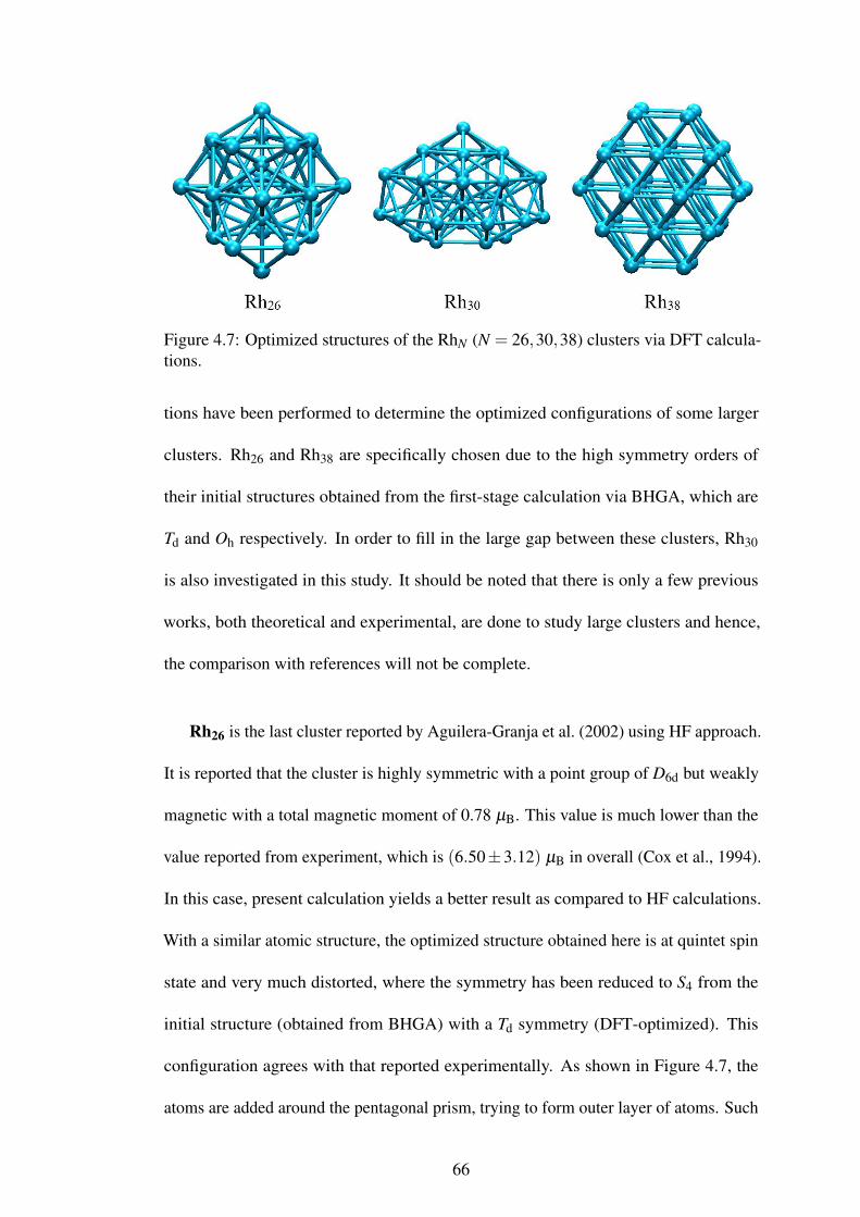
Figure 4.7: Optimized structures of the RhN (N = 26,30,38) clusters via DFT calcula-tions.

tions have been performed to determine the optimized configurations of some larger

clusters. Rh26 and Rh38 are specifically chosen due to the high symmetry orders of

their initial structures obtained from the first-stage calculation via BHGA, which are

Td and Oh respectively. In order to fill in the large gap between these clusters, Rh30

is also investigated in this study. It should be noted that there is only a few previous

works, both theoretical and experimental, are done to study large clusters and hence,

the comparison with references will not be complete.

Rh26 is the last cluster reported by Aguilera-Granja et al. (2002) using HF approach.

It is reported that the cluster is highly symmetric with a point group of D6d but weakly

magnetic with a total magnetic moment of 0.78 µB. This value is much lower than the

value reported from experiment, which is (6.50±3.12) µB in overall (Cox et al., 1994).

In this case, present calculation yields a better result as compared to HF calculations.

With a similar atomic structure, the optimized structure obtained here is at quintet spin

state and very much distorted, where the symmetry has been reduced to S4 from the

initial structure (obtained from BHGA) with a Td symmetry (DFT-optimized). This

configuration agrees with that reported experimentally. As shown in Figure 4.7, the

atoms are added around the pentagonal prism, trying to form outer layer of atoms. Such

66

a trend of how larger clusters get built up becomes more obvious as the number of

atoms increases, as in the Rh30. Although the optimized structure of Rh30 is highly

distorted with only a low order C1 symmetry, it can be seen clearly that the second

(outer) layer of Rh atoms are completed. In terms of total magnetic moment, Cox et al.

(1994) reported a value of (3.90±4.20) µB, which has a rather large error bar. Hence,

the value of 6 µB obtained from present calculation is consistent with that measured

experimentally.

The last and largest cluster calculated in present thesis, Rh38, is an interesting one

due to its high symmetry order. The geometry relaxation, nonetheless, does not result in

any distortion but left the cluster to maintain in regular truncated octahedron (Figure 4.7).

As mentioned previously, Rh clusters display the tendency to become weakly magnetic

as the number of atoms increases. Nonetheless, this is not the case as far as Rh38 is

concerned. The present calculation shows that this cluster has a total magnetic moment

of a whopping 30 µB. Such a large total magnetic moment is unexpectedly high. All

existing literature findings, both theoretical and experimental ones, point towards the

suggestion of a weakly magnetic state for Rh clusters more than 20 atoms. There is

currently no theoretical references in the literature that makes a similar claim, nor is

there any experimental work done to measure such prediction. The possible existence

of large magnetic moment hence serves a strong motivation for the further study of

large transition metal clusters and the interplay between the geometrical environment

and the nature of these clusters.

67

4.4 Conclusions

As a summary to this chapter, the optimized configurations of Rh clusters, of the

size up to 23 atoms, and selected size of 26-, 30- and 38-atom, are reported in full

detail. These configurations are generated without prior prejudice via a two-stage

computational procedure. In the first stage, BHGA, a powerful global minimum searh

algoritm is employed to obtain the ground-state structure of a cluster of a given size

in the PES of Gupta potential. The obtained cluster structures at the first stage are

then fed as input to the DFT code, deMon2K, to be locally optimized. The resultant

structures are then taken as the ground-state structures of the Rh clusters at the DFT

level. Comparisons between the ground-state configurations obtained by current work

against known theoretical and experimental results in the literature are also made and

reported. A good portion of the ground-state structures and magnetic moments obtained

from current calculations is consistent with that from existing literature, while the other

portion is not. The discrepancy could be due to the difference in the overall strategy

and methodology used, for example, the reliability of global minimal search algorithm,

variation in the nature of the numerical approach (for instance, HF against DFT), or the

procedural details of how the ground state configurations are generated as a whole. The

present thesis does not delve into explaining the technical details that give rise to the

discrepancy of the results as it is beyond its scope.

The results obtained from the current work show that for small-sized Rh clusters

of approximately less than 10 atoms, they display unique geometries. A trend of

icosahedral growth in the ground-state structures of the Rh clusters was found when

the size extents beyond approximately 13. The trend of the icosahedral growth is first

68

marked by the icosahedron at Rh13. The second checkpoint along the growth trend

is marked by the double icosahedron Rh19. The growth pattern continues in such a

way to form a second (outer) layer around the double icosahedron, which can be seen

clearly in Rh26 and Rh30. As an overall trend, the magnetism of Rh clusters is found

to become weaker as the cluster becomes larger, an observation which agrees with the

asymptotically expected fact that bulk Rh is paramagnetic. However, as an unique and

unexpected finding, calculation done in this work explicitly shows that Rh38, which is

in a regular truncated octahedral structure, has a whopping total magnetic moment of

30 µB, indicating the presence of interesting magnetic properties in large Rh clusters

worthy of further investigation.

69

CHAPTER 5

STRUCTURAL AND MAGNETIC PROPERTIES OF RHODIUMCLUSTERS

In this chapter, further analysis on the ground-state structures obtained in the

previous chapter will be performed and reported. Before studying the their structural

and magnetic properties, the optimized geometries as obtained in the previous chapter

are first reassured by subjecting them to a vibrational frequency analysis. Following

that, the size-dependent magnetism of rhodium (Rh) clusters is presented. The relative

stabilities as well as the structural properties of the clusters are also studied.

5.1 Vibrational Frequency Analysis

As discussed in Chapter 4, a candidate structure obtained from BHGA is fed into

the DFT package, deMon2k, to be geometrically relaxed without symmetry and spin

restriction. The optimized configuration is known as a stationary point on the potential

energy surface (PES). Right after the geometrically optimizing a cluster, it is usually

followed by vibrational frequencies calculation. Vibrational frequency calculation on

a stationary point is required in order to yield three important piece of information,

namely, (i) the nature of stationary point, (ii) the zero-point energy, and (iii) the infrared

spectra (Lewars, 2010).

Calculation of vibrational frequencies of a molecule involves finding the normal-

mode frequencies, which number of modes depends on the geometry of the molecule.

For a non-linear molecule with N atoms, it contains 3N−6 normal modes. On the other

70

hand, since the rotation about molecular axis does not produce a recognizable change

in the nuclear array, only two rotational vectors are subtracted for a linear molecule,

hence, it has 3N− 5 normal-mode frequencies. Suppose a dimer A–B has only one

normal-mode frequency, which is given by

ν =1

2πc

√kµ

(5.1)

where the vibrational "frequency" ν is actually a wavenumber, given in cm−1. The

constant c is the velocity of light and mr is defined as the reduced mass of the molecule,

mr =mAmB

mA +mB(5.2)

where mA and mB are the masses of atoms A and B respectively. The parameter k is the

force constant of a vibrational mode, which measures the "stiffness" of the molecule

toward that vibrational mode. In fact, as the frequency of a given vibrational mode is

related to the force constant for the mode, the directions and frequencies of the atomic

motions in a normal-mode vibration might be calculated from the force constant matrix,

which is also known as the Hessian (Lewars, 2010).

Consider a triatomic molecule, at which each of the atoms has a Cartesian coordinate

(x,y,z), yielding nine geometric parameters q1,q2, ...,q9. Here, the gradient matrix is

71

defined as the first-derivative matrix of energy of the system E,

g =

∂E/∂q1

∂E/∂q2

...

∂E/∂q9

(5.3)

and the second-derivative matrix is the Hessian (force constant matrix) which is given

by

H =

∂ 2E/∂q1q1 ∂ 2E/∂q1q2 ... ∂ 2E/∂q1q9

∂ 2E/∂q2q1 ∂ 2E/∂q2q2 ... ∂ 2E/∂q2q9

...... ...

...

∂ 2E/∂q9q1 ∂ 2E/∂q9q2 ... ∂ 2E/∂q9q9

. (5.4)

In general, when a given square, symmetric, matrix A is diagonalized, it is decomposed

into three square matrices which can be written as

A = PDP−1 (5.5)

where D is a diagonal matrix (all off-diagonal elements are zero), P is a premultiplying

matrix and P−1 is the inverse matrix of P. When this is applied to a physical problem,

the diagonal elements of D are the magnitudes of some physical quantity and each

column of P represents a set of coordinates which give a direction associated with

the physical quantity. Therefore, diagonalization of the Hessian matrix for a triatomic

72

molecule can now be written as

H =

q11 q12 ... q19

q21 q22 ... q29

...

q91 q92 ... q99

P

k1 0 ... 0

0 k2 ... 0

...

0 0 ... k9

k

P−1.(5.6)

From Equation (5.6), each column of P matrix is the "direction vector" for the vibration

whose force constants are given by the k matrix (Lewars, 2010). By Equation (5.6), the

force constant corresponds to a vibrational mode i, ki, can be derived if the Hessian is

known. Hence, in this way, frequencies of each vibrational mode can be calculated in

terms of the mass-weighted force constant as per Equation (5.1).

This section focuses only on the nature of stationary point of a given cluster, while

other information derivable from vibrational frequency analysis,such as the infrared

spectra and zero-point energy of the Rh clusters, which are not in the scope of this

thesis, are presented in the Appendix B. The nature of the stationary point specifically

refers to whether it is a minimum, a transition state (also known as first-order saddle

point), or a nth-order saddle point on the PES. In practice, the nature of a stationary

point is determined by checking the number of imaginary frequencies present in the

vibrational frequency calculation. At a local minimum on the PES, all force constants

of normal-mode vibrations are positive, and each vibrational mode in the molecule

is harmonic in this case. Hence, if the stationary point is indeed a local minimum,

vibrational frequency calculation should produce no imaginary frequency. On the

contrary, if the stationary point is a transition state, the vibration along the reaction

73

Figure 5.1: The figure on the right refers to a local minimum on a PES, while the lefta transition state. In the case of the right figure, the derivative of the gradient at thelocal minimum is positive, hence all of its normal-mode force constants are positive.Conversely, in the left figure, the surface curves down along the reaction coordinate atthe transition point, giving a negative force constant and consequently an imaginaryvibrational frequency.

coordinate is different than that of a local minimum. In this mode, the vibration is

no longer harmonic and eventually the molecule is changed to another configurations.

As shown in Figure 5.1, unlike a minimum that has a positive gradient (the surface

concaves upward), the surface along the reaction coordinate concaves downward. As

a consequence, the force constant, which is the first derivative of the slope, for this

mode is negative. From Equation (5.1), the frequency is hence an imaginary number.

In short, the nature of the stationary point can be distinctly recognized by determining

how many imaginary frequencies are present in the calculation: a local minimum has

only real-valued frequencies, while a transition state has one imaginary frequency. If

there exists n imaginary frequencies, it corresponds to the nth-order saddle point which

has n negative force constants in normal-mode vibrations.

In the present work, the optimized configurations are proven to be minima on

their respective PES, except three clusters: Rh12, Rh13 and Rh20. We shall discuss

these cases in turns. For Rh12, geometry optimization shows that the lowest-energy

structure happens at the multiplicity of 21, whose structure is as shown in Figure 4.4

74

Figure 5.2: Plot of relative energies for Rh13 against spin multiplicity. The initiallowest-energy configuration with multiplicity 22 is a transition state; while the nexttwo configurations in the 20-tet and 18-tet spin state are third- and second-order saddlepoints respectively. A cross in the plot at 16-tet spin state indicates the true minimumof Rh13

with a low symmetry order (Cs). However, since vibrational analysis yield an imaginary

frequency for the cluster with a multiplicity of 21, the true minimum is assumed by the

second-lowest-energy configuration with a lower magnetic moment of 18 µB.

For the case of Rh13, due to the existence of imaginary mode, the true minimum is

located at a spin state lower than that with a total magnetic moment of 21 µB, which is

initial determined to be the lowest-energy configuration. From present calculation, the

icosahedral structures of Rh13, as shown in Figure 4.4 with spin states of 22, 20, 18 and

16 are all distorted and have the same symmetry of D2h. Figure 5.2 is the plot of energy

variation of Rh13 across a wide range of multiplicity. Vibrational frequency calculation

indicates that the configurations with multiplicity 22, 20 and 18 are transition state,

third-order and second-order saddle points respectively. As a result, the true minimum

of Rh13 is assumed by the configuration with total magnetic moment of 15 µB.

75

For Rh20, calculation done in the present work shows that a triplet Rh20 is a transition

state. Thus, the next-lowest-energy structure at quintet spin state is assumed to be the

true minimum of the cluster. It should be remarked that the optimized configurations

reported in Chapter 4 are the true minima which have already been cleared of imaginary

frequencies.

5.2 Size-dependence Magnetism of Rhodium Clusters

One of the unique properties of nanoparticles, in particular in metallic clusters, is

its size-dependence magnetic property. For a 3d transition element such as Fe, it has

been shown that the magnetism of the cluster is enhanced when compared to its bulk

counterpart (Hafner & Spišák, 2007). As already mentioned in previous chapter, being a

4d transition metal, Rh is paramagnetic in bulk form. Theoretically and experimentally,

it has been shown that Rh is magnetic in reduced dimension (Cox et al., 1994; Reddy

et al., 1993).In this section, the calculated results on how magnetism of Rh cluster

varies across a range of sizes will be reported in a better detail than that preliminarily

mentioned in the previous chapter.

Figure 5.3 shows a plot of average magnetic moment of Rh clusters versus the size

of lowest-energy configurations. The plot has to be analysed in conjunction with the

geometry associated with each cluster size. Using the geometry of the cluster as a guide,

the plot can be roughly separated into three regions: The small-size region (defined

to be N ≤ 10 atoms), the intermediate region (defined to be 10 ≤ N < 19 atoms), and

large-size region with the range N ≥ 19 atoms).

In the small-size region the magnetism of the clusters fluctuates erratically. This can

76

Figure 5.3: Plot of average magnetic moment of Rh clusters against cluster size, whilethe values of the isomers of Rh4, Rh6 and Rh22 are indicated by the crosses in the plot.

be understood from the finding reported in previous chapter that each of the small-sized

cluster has their unique geometry. Magnetic moment fluctuation in the intermediate

region is relatively milder than that in the small-size region. This observation might be

linked to the finding that the geometries of the clusters are icosahedral-like (except for

Rh11, which is geometrically related to Rh9). The icosahedral growth patter ceases at

the double icosahedron Rh19, coincidental with the boundary between the intermediate

and large-size region.

The magnetic moment drops drastically at Rh19, at which the magnetism is almost

vanished, marking the transition into the large-size region. In this region, the clusters

are large in size but relative low in magnetic moment. This agrees with the previ-

ous findings, both theoretically and experimentally, that the clusters become weakly

magnetic when the number of atoms exceeds 20. Due to excessively expensive cost

in DFT computational, only four selected clusters with size beyond 23 are evaluated,

namely, Rh26, Rh30 and Rh38. These large clusters of selected sizes, despite limited

77

in number, will be used as a probe to tell us whether the magnetic trend also extends

into region with size much larger size than 19. In particular, Rh38, which is the largest

cluster probed in this thesis, displays a relatively high magnetic moment as compared

to other clusters in the large-size region in the plot. Nevertheless, magnetic moment in

the large-size region, including the Rh38 cluster, still has less than 1.00 µB/atom) of

magnetic moment. This trend is consistent with the expectation that when a Rh cluster

grows larger in size, its magnetic moment becomes increasingly weak, and eventually

vanishes at the bulk scale.

The results presented in this section establish the conclusion that the magnetic

moment of a Rh clusters in its ground state is indeed size-dependent. This conclu-

sion, which is arrived at via rigorous DFT calculations performed on the imaginary-

vibrational-mode-free ground-state structures of these clusters, makes a good agreement

with the previous findings that have been reported theoretically and experimentally.

The size-dependent properties of Rh clusters will be further analysed in the following

sections.

5.3 Relative Stability of Rhodium Clusters

In this section, energetic analysis is performed in order to investigate the stability of

the Rh clusters. To this end, the average binding energies (Eb), dissociation energies

(De) and second-order difference of energies (∆2E) are calculated. These quantities are

respectively defined respectively as follows:

Eb(RhN) =1N[NE(Rh)−E(RhN)], (5.7)

78

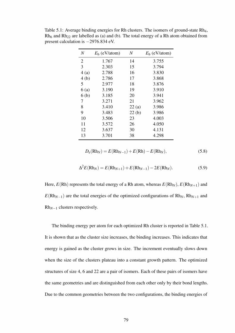
Table 5.1: Average binding energies for Rh clusters. The isomers of ground-state Rh4,Rh6 and Rh22 are labelled as (a) and (b). The total energy of a Rh atom obtained frompresent calculation is −2976.834 eV.

N Eb (eV/atom) N Eb (eV/atom)

2 1.767 14 3.7553 2.303 15 3.7944 (a) 2.788 16 3.8304 (b) 2.786 17 3.8685 2.977 18 3.8766 (a) 3.190 19 3.9106 (b) 3.185 20 3.9417 3.271 21 3.9628 3.410 22 (a) 3.9869 3.483 22 (b) 3.98610 3.506 23 4.00311 3.572 26 4.05012 3.637 30 4.13113 3.701 38 4.298

De(RhN) = E(RhN−1)+E(Rh)−E(RhN), (5.8)

∆2E(RhN) = E(RhN+1)+E(RhN−1)−2E(RhN). (5.9)

Here, E(Rh) represents the total energy of a Rh atom, whereas E(RhN), E(RhN+1) and

E(RhN−1) are the total energies of the optimized configurations of RhN , RhN+1 and

RhN−1 clusters respectively.

The binding energy per atom for each optimized Rh cluster is reported in Table 5.1.

It is shown that as the cluster size increases, the binding increases. This indicates that

energy is gained as the cluster grows in size. The increment eventually slows down

when the size of the clusters plateau into a constant growth pattern. The optimized

structures of size 4, 6 and 22 are a pair of isomers. Each of these pairs of isomers have

the same geometries and are distinguished from each other only by their bond lengths.

Due to the common geometries between the two configurations, the binding energies of

79

Figure 5.4: Second-order energy differences (upper) and dissociation energies (lower)for Rh clusters against cluster size, while those values of the isomers of Rh4, Rh6 andRh22 are indicated by the crosses in the plots.

a pair of isomers are close to each other. The closeness in binding energies between the

isomer pairs are indicated by the parenthesis (a) and (b) in Table 5.1.

In general, the stability of a cluster with respect to its neighbours is quantified

by the second-order difference in the energies between the cluster and its neighbours.

80

Figure 5.4 illustrates the variations of the ∆2E values with the size of the Rh clusters,

up to Rh22. A high peak of this plot indicates higher relative stability of the respective

cluster. The results of the present calculation show that ∆2E fluctuates between the

odd and even cluster size. Rh14, which is in the region between Rh11 and Rh16, has a

particularly high relative stability. Nevertheless, Rh clusters with even number of atoms

are found to be more stable than those with odd number of atoms.

Figure 5.4 also shows the variation of the dissociation energies of Rh clusters, De,

which is another indicative measurement of relative stability. In this context, high De

value implies a high chemical stability of the cluster. From the graph, it is shown that

local peaks happens more often at the even-numbered clusters, as compared to the

odd-numbered cluster. Besides, this measurement also shows that the clusters sized

between 11 to 17 are thermodynamically stable with respect to their neighbours. The

odd-even staggering pattern in De is similar, and hence, consistent with the findings

from the calculation for ∆2E.

5.4 Structural Properties

Investigation of the structural properties of a cluster is an integral part of the

current thesis as it might provide further insight into the influence of the geometrical

environment of the cluster. For a bulk system, the structural properties are quantified

in terms of lattice constant, bulk modulus and cohesive energy. On the other hand,

for a non-periodic cluster system, its structural properties are quantified in terms of

interatomic distances and molecular symmetry.

As reported in the previous chapter, the optimized structures of Rh clusters generally

81

Figure 5.5: Plots of average binding energies (orange) and radial bond distance (green)for Rh clusters against cluster size. The values of the isomers of are indicated by theblue and red crosses.

have closed geometries. All the optimized clusters reported in this thesis are generally

small clusters in approximately spherical shape irrespective of their symmetry group. It

is hence deemed feasible to calculate the average radial bond distances for these clusters

within the limit of this approximation. Suppose one of the atom in the cluster, labelled

with index i, is located at Cartesian coordinate (xi,yi,zi), while the centre of mass of the

cluster (xc,yc,zc). The radial bond distance of atom i is defined as the distance between

these two points. For a N-atom cluster, its average radial bond distance can be written

as

d =1N

N

∑i=1

di. (5.10)

In the previous section, the calculation of binding energies shows that a Rh cluster gains

energy as it grows in size. Figure 5.5 compares the plots of average binding energy

and average radial bond distance against the cluster size. It is found that both plots

exhibit similar growth pattern: The plots increase rapidly in the small-sized region but

82

Figure 5.6: Plot of average nearest-neighbour distance of Rh clusters against clustersize, while the values of the isomers of Rh4, Rh6 and Rh22 are indicated by the crossesin the plot.

the increment slows down from Rh11, where the icosahedral growth starts.

However, there is a small plateau between Rh11 and Rh13 happening in the average

radial bond distance but not in binding energy plot. The small plateau in the radial bond

plot can be understood from the context that the clusters in this plateau is still in the

process of completing an icosahedron. As a result, the radius of the structure remains

relatively constant. On the other hand, the gradual gaining of energy in this small

plateau region can be understood from the context that energy increases monotonically

as atoms are consecutively added to the current structure.

This thesis has also attempted to calculate the average nearest-neighbour distances

of the optimized clusters. The obtained theoretical results are presented in Figure 5.6

and apparently, the average nearest-neighbour distances of Rh clusters are also size-

dependent. The distances between an atom with its nearest neighbour in small clusters,

83

up to 6 atoms, increases rapidly. The trend is then followed by a fluctuating region

between Rh7 and Rh17, and eventually this quantity converges to a value of 2.57 Å at

Rh26.

At this point, the behaviour of nearest-neighbour distance against Rh cluster size as

obtained here is compared to that in Aguilera-Granja et al. (2002). In Aguilera-Granja

et al. (2002), the authors, by observing their plot of average nearest-neighbour distance,

suggested that at the size of around Rh13, the nearest-neighbour distance has already

converged to that corresponds to the bulk value, 2.69 Å, measured by a very early paper

(Kittel & Holcomb, 1967). In the present plot, the nearest-neighbour distance flattens

into a plateau of 2.57 Å as the cluster size enters the range of Rh18−Rh26, suggesting

that the bulk nearest-neighbour distance inferred from the present calculation is 2.57

Å instead, which is only approximately 4% of discrepancy to that measured in (Kittel

& Holcomb, 1967).

The strong dependence of magnetism of a cluster on its local geometry, in particular

its nearest- and second-nearest-neighbour distances, is suggested by Di Paola et al.

(2016). Therefore, it is tempted to compare the trends in the magnetism and average

nearest-neighbour distances curves of the Rh clusters, Figure 5.3 and Figure 5.6.

The first observation from the comparison is that the clusters in the convergence

region (Rh18−Rh26), with the exception of Rh18, are weakly magnetic. On the other

hand, it is also known that bulk Rh, which nearest-neighbour distance coincides with

that in this plateau region is paramagnetic (Lide, 2000). The second observation from

the comparison is that there are two peaks on the nearest-neighbour plot, located

84

Table 5.2: Symmetry order of each point group. The subscript n indicates the order ofrotation axis.

Group Symmetry Symmetry Order

Linear C∞v, D∞h ∞

Non-axial Cs 2

AxialCn, Sn nCnv, Cnh, Dn 2nDnd, Dnh 4n

Cubic Td 24Oh 48

Icosahedral Ih 120

respectively at Rh7 and Rh38, where their values are much larger than the assumed bulk

value. Coincidently, the optimized configurations of these two clusters as obtained in

this calculation are found to have relatively high magnetic moment than their neighbours.

These two accidental coincidences, which are observed based on limited data analysis,

may hint on a non-trivial correlation between the local geometry of a cluster and its

magnetic properties, as suggested by Di Paola et al. (2016).

In the studies of theoretical physics and chemistry, symmetry is an integral aspect

to consider when studying the structural properties of a material at atomistic level. In

crystallography, the symmetry of a crystal is described by space groups. However,

translational symmetry, which is part of space groups, does not exist in finite system

such as molecules or clusters. The symmetry of a finite system is instead described by

point groups. As the name suggested, whenever there is a symmetry operation applied

to a cluster, at least one point is not affected. Symmetry of a cluster is expressed in

standard symbol, for example Ih for icosahedral symmetry and C5 for a simple fifth

order of rotational symmetry. The order of symmetry is a numerical integer used to

quantify a point group. Symmetry order is determined by counting the number of

85

symmetry elements in the respective point group. The higher the symmetry order of a

point group, the larger is its number of symmetry elements. With the use of symmetry

order, quantitative comparison between two point groups becomes straight forward.

For example, consider two clusters. One has an icosahedral point symmetry Ih with a

symmetry order of 120, whilst the other has a cubic Td symmetry with a symmetry order

of 48. Thus, the Ih cluster is ranked higher in terms of symmetry because its symmetry

order is larger (120) than that of the Td cluster (48). Symmetry order of all point groups

is summarized in Table 5.2.

In the process of geometrically optimizing a candidate structure (which is obtained

from BHGA in the first of the two-stage computational procedure) by DFT (i.e. the

second of the two-stage procedure), the interatomic distances of the candidate structure

are to be fully relaxed. Hence, the symmetry of the candidate cluster in principle could

be altered after the optimization. Figure 5.7 shows a plot that compares the symmetries

of the clusters before and after geometrical optimization by DFT. It is seen that the

symmetries of optimized Rh clusters (red in colour) either remain unchanged or become

lowered as compared to the initial structures (green in colour), except Rh9 which

becomes more symmetric than the input configuration. The plot also shows that Rh6

and Rh38 are relatively stable during geometry relaxation by DFT since both clusters

remain at octahedral symmetry (Oh). On the other hand, the highly symmetric initial

configuration of Rh13 is unstable in the optimization as later the final configuration

becomes a distorted icosahedron with D2h.

The relationship between magnetism of clusters and molecular symmetry has been

studied by Dunlap (1990) and T.-W. Yen and Lai (2016). The former work claims

86

Figure 5.7: The upper graph compares symmetry order of initial (green) and optimized(red) configurations of Rh clusters, while the values of the isomers are indicated byorange triangle and blue cross symbols respectively. The lower graphs displays theaverage magnetic moment (grey) and symmetry order (blue) of optimized Rh clustersagainst cluster size, while the values of the isomers of are indicated by the orange dotand red cross symbols respectively.

that a cluster with higher symmetry order like Ih has a larger magnetic moment. On

the other hand, the authors of T.-W. Yen and Lai (2016), by varying the composition

of bimetallic clusters of noble metals, find that small magnetic moments are induced

in highly symmetric clusters. In the present study, the magnetism of Rh clusters are

87

compared with corresponding symmetry orders and plotted against the cluster size in the

lower graph of Figure 5.7. For clusters with less than 10 atoms, the relationship between

magnetism and symmetry order is antagonistic: clusters with higher symmetry have

lower magnetic moment. For instance in the case of Rh4, where a pair of isomers are

found at its lowest-energy state, a Td structure is non-magnetic but a S2d structure has a

total magnetic moment of 6 µB. For clusters in the size of Rh19 to Rh30, the symmetry

orders range at at relatively low value, i.e. from one to five. Clusters in this range are

weakly magnetic. The largest cluster studied in this work, Rh38, is highly symmetric

and has a relatively large magnetic moment (total of 30 µB). Similar observation is

found in the small cluster Rh7 (total of 13 µB), which is both high in magnetic moment

and symmetry order. Based in the findings of the present thesis, Rh clusters are not

necessary highly magnetic even if they are highly symmetric.

In a nut shell, structural properties of Rh clusters are studied by investigating the

geometrical environment of the clusters. It is shown that as the cluster size becomes

larger, in terms of the radial bond distance, the cluster gains energy and hence, results

in the increase of binding energy. While the average nearest-neighbour distance of

Rh clusters converge to that of the bulk value, the clusters become weakly magnetic.

Moreover, the symmetry of a candidate cluster is either remained unchanged or reduced

after geometrical optimization by DFT framework. As far as Rh clusters are concerned,

a highly symmetric cluster is not necessary strongly magnetic. This is especially true

for small cluster. Evidence of definitive correlation between symmetry (and nearest-

neighbour distance) and magnetism in Rh clusters is at best partial, but far from

conclusive.

88

CHAPTER 6

ELECTRONIC STRUCTURES OF RHODIUM CLUSTERS

DFT calculations has included quantum mechanical contributions from the electrons

in the system being considered. As reported in the previous chapters, it has been shown

that the geometry of a candidate cluster could undergo alteration after being DFT-

optimized, on top of the observation that magnetic and structural properties of the

rhodium (Rh) clusters display size-dependence behaviour. In this chapter, electronic

structures of rhodium (Rh) clusters will be discussed in details, including the electronic

stability of the clusters, as well as the distributions of charges and spins in the clusters.

6.1 Molecular Orbitals

An atomic system like the hydrogen atom consists of only a single electron. The

one-electron wavefunction of this system is called the atomic orbital. Whereas in

a molecular system, the atomic orbitals of each atom overlap when two atoms are

brought to a certain distance. In this case, the probability to find the electrons from both

atoms in this overlapped region becomes remarkable and thus, molecular orbitals are

formed. Homologous to the atomic system, these orbitals represent the many-electron

wavefunctions of a molecular system. In molecules, the electrons are supposed to move

around in the field contributed by all nuclei and other electrons. The molecular orbitals

are obtained from the linear combinations of atomic orbitals (LCAO), as stated in in

Equation (3.39).

89

Figure 6.1: (a) Occupation of spins in a restricted (spin-unpolarized)formalism, and (b)occupation of spins in an unrestricted (spin-polarized) formalism.

In DFT calculations, the choice of basis set is very crucial as it determines the

forms of molecular orbitals. When the molecular orbitals are known, the electrons are

arranged accordingly with ascending energies of spin orbitals and finally, the electronic

configurations and properties of the molecule are established. A spin orbital (χ) is

defined as the product of spatial orbital (ϕ) and a spin function (which could be a spin

up function (α) or a spin down function (β ). In general, α-spin and β -spin orbitals are,

respectively, written as

χ↑(x) = ϕ

↑(r)α(ω)χ↓(x) = ϕ↓(r)β (ω) (6.1)

where x = (r,ω), while r and ω are spatial and spin coordinates respectively (Skylaris,

2016).

The energy of a spin orbital (ε) depends on the KS formalism used in the calculation,

which can be either a restricted or an unrestricted formalism. In the restricted (spin-

unpolarized) formalism, the orbitals of up (α) and down (β ) spins have the same spatial

orbital ϕ , i.e. ϕ↑ = ϕ↓ = ϕ . As a result, both spin orbitals have the same energy values.

On the other hand, the α and β spins in the unrestricted (spin-polarized) formalism are

allowed to occupy different spatial orbitals (ϕ↑ 6= ϕ↓). As a results, their energies are

90

different. Figure 6.1 illustrates schematically the difference in spin occupation between

two methods.

In this thesis, the clusters being considered comprise of different number of atoms

that could form both open- and closed-shell systems. Therefore, the unrestricted

formalism is adopted so that a consistent treatment is applied to all cluster sizes,

irrespective of whether they are open- or closed-shell systems.

The basis set employed in spin-unrestricted calculation is known as LANL2DZ.

There is a total of 17 valence electrons from each Rh atom. Figure 6.2 presents the

occupancies of all valence electrons in a Rh atom in spin-polarized calculations.

Each horizontal line in Figure 6.2 represents an energy level. Each arrow represents

a spin; up arrow represents up (α) spin, while down arrow represents down (β ) spin.

All energy levels in Figure 6.2 that are occupied by two arrows are degenerate states,

e.g., χ↑8 = ϕ

↑8 α and χ

↑9 = ϕ

↑9 α in Figure 6.2. Both spin orbitals are represented by a

single energy level labelled ϕ8,9 in the left column of Figure 6.2. For example, the

energy level of highest occupied α spin orbital (ϕ8,9) is said to be doubly degenerate as

it could be occupied by two electrons.

It can be observed that overall, β spin orbitals always have higher energies than

their respective α spin orbitals. Electrons first fill up the lowest-energy α spin orbital.

The orbital that is filled at the last ends at the β spin orbital with an energy of −3.86

eV. The highest occupied α spin orbital is that labelled φ8,9 in the left column of

Figure 6.2, whereas the highest occupied beta spin orbital is that labelled φ8 in the

right column, where the orbital φ9 in the degenerate φ8,9 orbitals is unoccupied. As

91

illustrated in Figure 6.2, the arrangement of electrons in Rh atom results in a net spin

angular momentum of S =12

, originating from the unpaired α spin in ϕ9. The net spin

magnetic moment of a particle with a net spin angular momentum S is given by µ = 2S

µB. Hence, the net spin magnetic moment of a Rh atom is 2S = 2× (+1/2) µB = 1 µB.

From Figure 6.2, the spin states that are occupied by first 8 valence electrons in an

atom are very low in energies, compared to the remaining 9 electrons occupying the

higher energy states. When a molecule or a cluster is formed, those 9 electrons have a

higher chance to overlap with electrons from another atom. Consider a Rh dimer as an

example. It has a 9+9 = 18 high-energy states valence electrons (9 from each atom)

and 8+8 = 16 low-energy states valence electrons (8 from each atom). The molecular

orbital energy diagram for the 18 high-energy states valence electrons of the dimer

is demonstrated in Figure 6.3. From the output of DFT calculation by deMon2k, the

highest occupied α-spin orbital is χ↑19 (indicated in Figure 6.3 as a crossed red dot),

while the highest occupied β -spin orbital is χ↓15 (indicated in Figure 6.3 as a crossed

blue dot). Hence, there exist 19−15 = 4 unpaired α spin electrons in the dimer. This

is translated into a net spin of S = 4× (+1/2) = 4/2, which is equivalent to a net

magnetic moment of µ = 2S µB = 4 µB. The dimer hence is in a quintet spin state (spin

multiplicity of five). It is reminded that spin multiplicity M and net spin S is related by

the relation M = 2S+1.

The energy levels correspond to HOMO and LUMO are also indicated in Figure 6.3.

The HOMO level corresponds to α spin with ϕ19, whereas the LUMO level corresponds

to α spin with ϕ20. The HOMO-LUMO gap of the Rh dimer is the energy difference

between these two levels, which turns out to be 1.96 eV.

92

Figure 6.2: Atomic orbital energy of Rh atom in unrestricted calculations. Occupiedα (β ) spin orbitals are indicated by solid up (down) arrow, whereas unoccupied spinorbitals are indicated by dashed arrow. The spatial orbital of ith α (β ) spin orbital isindicated by ϕi on the left (right) of the occupancies and its energy is stated in bracketswith unit of eV. The energy level is not plotted according to real scale.

93

Figure 6.3: Molecular orbital energy of Rh dimer in unrestricted calculations. Theenergy of a spin orbital is in eV unit and its axis is shared between two spin states.Occupied spin orbitals are indicated by solid lines, whereas unoccupied spin orbitalsare indicated by dashed line. Red dots represent α-spin states. Green dots representβ -spin states. Only 9+9 = 18 valence electrons from higher energy spin orbitals arerepresented. The highest occupied α-spin orbital is χ

↑19 (indicated as a crossed red dot),

while the highest occupied beta-spin orbital is χ↓15 (indicated as a crossed blue dot).

94

Figure 6.4: Plot of HOMO-LUMO gaps of Rh clusters against cluster size, while thevalues of the isomers of Rh4, Rh6 and Rh22 are indicated by the crosses in the plot.

6.1.1 Electronic Stability

In the previous chapter, stability of a cluster is studied via energetic analysis, which

is originated from the geometrical aspect. The stability of a cluster can also be studied

from its electronic structure, through the value of its HOMO-LUMO gap.

Figure 6.4 presents the variation of HOMO-LUMO gap with cluster size. There are

several significant high peaks with energy difference of more than 1 eV, which occurred

at the Rh dimer, trimer, Rh7 as well as Rh12. The large HOMO-LUMO gaps indicate

that these clusters are chemically more stable and thus, less reactive than other clusters.

It is also found that the isomers (indicated as crosses) of Rh4 and Rh6, where both are

in septet spin state, are more stable than their non-magnetic configurations (indicated as

dots). For clusters with more than 15 atoms, the results show that the energy values of

their HOMO and LUMO are close to each other and therefore, the large Rh clusters are

chemically unstable compared to the small clusters.

95

6.2 Population Analysis

The previous section discusses how the electrons in a cluster arrange themselves

in the molecular orbitals. This section will in turn discuss how the electrons distribute

among themselves over the optimized Rh clusters in three-dimensional space. It is

important in the fundamental study of quantum chemistry to know the distribution of

charges and spins in Rh clusters and which individual atom contributes to the peculiar

magnetic behaviour of the clusters. Distribution of electronic charges and spins in a

cluster can be obtained via population analysis. Both are very useful quantum chemistry

information. Atomic partial charges, which are not a physical observable, can be derived

from population analysis by partitioning the total electron density.

In the literature, various methods have been suggested for population analysis. Each

available method is based on its own respective idea and results obtained from different

methods in general are not completely comparable. In practice the choice of population

analysis method is a matter of preference or convenience, as the "the-most-appropriate"

method may depend on the system to be analysed on a case-by-case basis.

Three of the most well-known schemes for population analysis are Mulliken, Löwdin

and natural bond order analysis. Among these methods, Mulliken population analysis is

the most conventional method and included in most of the DFT software packages. This

oldest method of population analysis equally distributes the electrons in overlapped

region between two atoms. Due to the oversimplified treatment, charge distribution

pattern obtained from this scheme could become unreliable with increasing basis sets.

Löwdin method, which is an improvement based on Mulliken scheme, is made as the

choice of the population analysis scheme in this thesis.

96

6.2.1 Löwdin Populations

Unlike Mulliken, Löwdin-scheme does not take into account the overlapped popula-

tions. It is based on the idea that orthonormal basis functions do not overlap. Löwdin

transforms the atomic orbital basis functions into an orthonormal set of basis functions

before the analysis is performed. Consequently, calculations on overlapped populations

can be avoided, yet the charges of individual atoms would be more reliable with a larger

basis set (Springborg, 2000).

6.2.2 Charge Distribution of Rhodium Clusters

In a neutral cluster, electrons are not necessarily distribute uniformly around every

atom. In fact, the electrons may preferably stay at some favourable sites (resulting in

negatively charged atomic sites), while leaving some atomic sites to have excessive

positive charges. No matter how the charges are distributed, a neutral cluster, by

definition, will has no overall net charge. The charge distribution diagrams of Rh

clusters obtained from present analysis are presented in Figure 6.5.

In small Rh clusters up to Rh6, all atoms generally remain neutral. Although there

is a positively charged vertices in Rh5, the magnitude of charges is negligible. The first

cluster that has a distinctively non-zero distribution of charges is Rh7, in which there is

a discrepancy of charges between the pentagonal plane to the two vertices of bipyramid.

Next, the charges of Rh8 are concentrated on the bent rhombus. Since the optimized

structures of Rh9 and Rh11 are closely related (double octahedron and bicapped double

octahedron, respectively), both of them have negatively charged triangular plane which

connects two octahedron.

97

It is shown that the distribution in Rh10 is similar to those in Rh12 and Rh13 clusters.

Here, the central atom of each cluster is negatively charged while the surrounding atoms

have a small magnitude of positive charges.

While the icosahedral growth continues in following clusters, two main in the

distribution pattern occurred. Firstly, with reference to icosahedral structure, the vertex

atom which is close to the capped atoms becomes negatively charged. Secondly, the

pentagonal plane between central atom and the vertex atom progressively becomes

neutral. When the cluster size arrives at Rh19, the vertex atom of icosahedron becomes

the second largest negatively-charged inner atom. The charges are distributed evenly

between the upper and lower parts of double icosahedron, neutralizing the connecting

pentagonal plane.

As the icosahedral growth is continued to large Rh clusters, the charges get dis-

tributed following the pattern discussed above. Eventually, the charges of Rh26 are

concentrated on the four inner atoms, surrounded by positively charged atoms. While

for Rh30 , the electrons do not concentrate on the central atom of the bicapped pentago-

nal prism, but they stay in two atoms located between the central atom and the outer

layer of the structure. Lastly, the electrons of Rh38 are concentrated mainly on inner

rhombohedron, followed by central atom of each hexagonal face, leaving the edges of

hexagonal faces to be positively charged.

To summarize, the present Löwdin population analysis shows that the electrons of

Rh clusters have the tendency to migrate from outer to inner atom sites as the cluster

size grows. The charges are also more concentrated on the atoms which have higher

98

coordination number, i.e. atoms with more nearest neighbours. As there is lack of

detailed charge distribution of Rh clusters reported in the literature, the present results

are compared with the distributions of other metallic clusters. The trends of distribution

obtained make good agreement with previous studies which claimed that the charges

of metallic clusters are more likely to stay in the interior of the structures (T.-W. Yen

& Lai, 2016). Although there are references like Cerbelaud, Ferrando, Barcaro, and

Fortunelli (2011) that suggested the opposite way, the results are not comparable as the

methods employed are different.

99

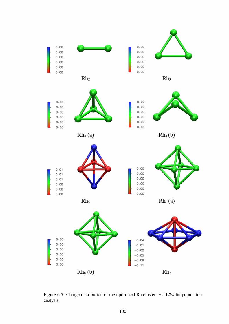
Figure 6.5: Charge distribution of the optimized Rh clusters via Löwdin populationanalysis.

100

Figure 6.5: Charge distribution of the optimized Rh clusters via Löwdin populationanalysis.

101

Figure 6.5: Charge distribution of the optimized Rh clusters via Löwdin populationanalysis.

102

Figure 6.5: Charge distribution of the optimized Rh clusters via Löwdin populationanalysis.

103

6.2.3 Spin Distribution of Rhodium Clusters

This section will report on the distribution of spins in the Rh clusters obtained from

population analysis. This information is particularly important in the study of magnetic

property because it allows one to determine the magnetic ordering of the cluster. The

spin distribution diagrams of Rh clusters obtained from Löwdin populations are shown

in Figure 6.6.

From Rh dimer to Rh7, the spins are equally distributed among the atoms. Even

though the distribution diagrams show different colouration of atoms on some of these

magnetic clusters, the differences in magnitude of spins are insignificant.

As the calculations are performed in a spin-unrestricted condition, the results show

that the distribution of spins in Rh clusters does not have a fix pattern. To illustrate this

statement, Rh10, Rh12 and Rh13 are taken as examples. Although these clusters grow in

such a way towards the formation of icosahedron, their spins are distributed in different

pattern. For Rh10 and Rh12, the vertex atoms have spins with greatest magnitude. Yet,

the atom with largest spin magnitude of Rh13 is located at the centre of icosahedron.

The most remarkable findings from the spin distributions of Rh clusters is the

appearance of spin-down configurations. Rh9 is the first cluster obtained from this

analysis which consists of atoms with down-spin. These atoms are located on the plane

connecting two octahedrons. Unlike the distribution in Rh9, the down spins pf Rh11 are

located at one of the capped atoms of the double octahedron and its neighbouring atom.

Next, Rh16 has three spin-down atoms which are capped to an icosahedron. Up to this

end, Rh19 is the most significant antiferromagnetic structure. As shown in the diagram,

104

the up- and down-spins are separated clearly by a pentagonal plane without net spin.

Moreover, from Rh19 to Rh23, as well as Rh26 and 30, all of these clusters have atoms

with negative spins. Because of the spin-down atoms, the overall magnetic moment of

the clusters are lowered. Therefore, the optimized configurations of these clusters are

weakly magnetic.

In short, the spin distribution obtained from the population analysis has provided

information of magnetic ordering on Rh clusters. It is shown that most of the clusters

with number of atoms not more than 18 as well as Rh38 are ferromagnetic, where all of

the atoms have positive spins. The exceptional cases happen on Rh9, Rh11 and Rh16

clusters as there exist atoms with negative spins. The most interesting finding from this

analysis is the antiferromagnetic behaviour of Rh19. Also, the existing of spin-down

atoms in large clusters has explained the weak magnetic moment existed with these

clusters.

105

Figure 6.6: Spin distribution of the optimized Rh clusters via Löwdin populationanalysis.

106

Figure 6.6: Spin distribution of the optimized Rh clusters via Löwdin populationanalysis.

107

Figure 6.6: Spin distribution of the optimized Rh clusters via Löwdin populationanalysis.

108

Figure 6.7: Spin distribution of the optimized Rh clusters via Löwdin populationanalysis.

109

CHAPTER 7

CONCLUSIONS AND FUTURE STUDIES

This chapter concludes the results obtained from present calculations and highlights

important findings of the project. It is followed by some suggestions on research that

could be carried out in the future to further the understandings in Rh clusters.

7.1 Conclusions

When material is reduced from bulk into the size at atomic dimension, the resultant

atomic clusters exhibit unusual size dependence behaviour.

This thesis attempted a detailed study on the clusters of a selected element, namely,

rhodium (Rh), with sizes up up to 23 atoms. To explore larger clusters that are rarely

reported previously, clusters with 26, 30 and 38 atoms are selectively chosen for the

study. The ultimate goal of this project is to investigate the structural and magnetic

properties of Rh clusters at lowest energy state, i.e. ground-state configurations. Ground

state is the most essential piece of physical information in theoretical study of atomistic

systems, such as a cluster, as all physically-relevant observables that can be measured

experimentally, can be derived from the knowledge of it.

To initialise the study of Rh clusters, their ground-state structures must be first

made available. Experimental measurements to determine the ground-state geometries

of clusters are not common at small due to demanding precision and difficulty in the

manipulation of the nanoscale particles. Even if available, these measurements are only

110

for certain popular elements, and mostly for really huge-sized ones. However one can

theoretically generate the ground-state structures using some educated means without

experimental input. In many theoretical studies of clusters physics, the ground state

structures are obtained from experimental suggestions, while others construct them

artificially for example, by way of building cluster geometries from a seed unit based

on prescribed geometric rules. Meanwhile there are also research papers that apply

a large-scale screening strategy whereby they scan through databases or collections

of possible structures possibly available, and then locally optimize them one-by-one.

In this thesis, in order to obtain the ground-state configurations of the Rh clusters at

DFT level, a robust, unbiased search strategy is adopted. The search is carried out via a

two-stage computational strategy. The first of the two-stage computational procedure is

performed by deploying a global minimum search algorithm which couples canonical

Monte Carlo basin hopping (BH) with genetic algorithm (GA). The code used in this

thesis for the global minimum search is known as PTMBHGA, which is made available

to us by the courtesy of the Complex Liquids Laboratory from the National Central

University, Taiwan. In PTMBHGA, the search begins by initialising a series of same-

size cluster configurations. Based on a predefined merit function which makes use of

the empirical Gutpa potential as the energy calculator, PTMBHGA will then optimize

the individuals generated in each generation, via the built-in GA and BH algorithms,

towards the global-minimum of the potential energy surface (PES) of Gupta potential.

The configurations obtained at this stage are only the global minima in the PES at the

empirical level, not that at the DFT level which are the desired structures sought after

by this thesis. To obtain these, the optimized configurations at the Gupta PES are then

locally re-optimized via first-principles DFT calculations without spin and symmetry

111

constraints. This constitute the second of the two-stage computational procedure for

obtaining lowest-energy structures of the Rh clusters at DFT level.

Direct search for global minima via unbiased global search at the DFT level is very

costly, and it is relatively rare to find in the literature research papers reporting their

structures using such approach. The two-stage computational strategy adopted in this

thesis provides a convenient and pragmatic route, if not an entirely accurate one, to

circumvent the computational bottle neck presented by the costly DFT calculation (as

energy calculator). As a measure to verify whether the two-stage procedure produces

reliable global minimum structures, this thesis has attempted various checks and com-

parison against the available structures reported in the literature. As a conclusion, the

comparison results show that many of the structures obtained from this work agree well

with that obtained from the literature, while some are not. However, the results of the

comparison has to be interpreted with a grain of salt as non-trivial technical differences

in computation methods and procedures used (such as the choice of basis set, theoretical

framework or the robustness of global search algorithm used), could lead to variations

in the structures obtain.

For the first time, the ground-state structures of a few relatively large sized Rh

clusters are reported by this thesis, namely Rh26, Rh30, and Rh38. These structures have

rarely been reported in the literate, as far as shown by an exhaustive literature search

conducted during the working of this thesis.

In addition, the DFT-optimized configurations obtained in this work are subjected

to vibrational frequency analysis to confirm whether they are true minima or transition

112

states. After subjecting the DFT-optimized Rh clusters to comparison against that from

the literature and vibrational frequency analysis, the true minima structures are then

brought forward to be studied for their properties of interest.

The imaginary-vibration-mode-free DFT-optimized Rh configurations, along with

their respective associated magnetic moment, are reported in Chapter 4. The results

show an icosahedral growth pattern as the cluster increases in size. The first icosahedron

is completed at Rh13 followed by double icosahedron at Rh19. The growth pattern

continues to large clusters and eventually a truncated octahedron is formed with 38 Rh

atoms. The icosahedron growth pattern can be vividly visualised in Figures 4.4 to 4.7.

It is to be noted that such an ecstatically symmetric growth pattern is not a result of

artificial construction but rather one produced by the unbiased, two-stage computational

procedure starting from an initial random geometry. The finding of the symmetric

growth pattern is not likely a numerical coincidence due to its geometrical non-triviality.

Moreover, the growth pattern observed in this thesis has also been reported in the

literature for Rh clusters. Nevertheless, the individual structures obtained in this thesis

fit the icosahedron growth pattern in a much robust manner than that reported in the

literature, which contain a relatively larger number of exception cases to the growth

pattern. Confirmation of the icosahedral growth pattern in the ground-state structures

of Rh clusters up to 38 atoms in size with improved robustness is hence yet another

important finding of this thesis.

The present thesis has also demonstrated explicitly that structural and magnetic

properties of the Rh clusters are size-dependent. The details are reported in Chapter 5.

The plot of size-dependence magnetic properties of Rh clusters is shown in Figure 5.3,

113

which is roughly categorised into three regions: (i) small-size region (Rh2−Rh10)

where the magnetic moments fluctuate erratically, (ii) intermediate region (Rh11−Rh18)

with mild fluctuation, and (iii) large-size region (Rh20 - Rh30) where the clusters are

weakly magnetic. One of the remarkable findings in this thesis is the unexpectedly

high total magnetic moment of Rh38 since large Rh cluster is expected to be weakly

magnetic. In addition, energetic analysis performed on the DFT-optimized Rh clusters

shows that those with even number of atoms are relatively more stable than those with

odd number of atoms.

This thesis has also performed DFT calculations to study the electronic structures

of Rh clusters, in which how the electrons are distributed over the clusters and how they

fill up the energy states in the molecular orbitals are calculated. Details of the results

are reported in Chapter 6. Chemical stability of the clusters are accessed by analysing

their respective HOMO-LUMO gap, which are derived from the energy levels of the

molecular orbitals. The HOMO-LUMO gap as a function of cluster size is shown in

Figure 6.4. The results show that Rh2, Rh3, Rh7 and Rh12, as well as the magnetic

isomer of Rh4 are relatively more chemically stable than other cluster sizes.

Results on the charge distribution of electrons, calculated based on the Löwdin

population analysis scheme, are shown in Figure 6.5. The population analysis also

produces result of electron spin distribution over the clusters as in Figure 6.6. Overall,

the result of population analysis suggests that the electrons in the studied Rh clusters

prefer to stay at inner atoms, leaving the outer layer positively-charged. Previous works

reported that Rh clusters are mostly ferromagnetic. On the contrary, based on the results

of spin distribution obtained in this thesis, it is found that negative spins exist in small

114

clusters, i.e. Rh9 and Rh11. Negative spins are also found in the clusters with more

than 19 atoms (except Rh38). The existence of negative spin states results in weak

magnetization in these clusters. The weak magnetization as found in these few cases are

rarely reported previously, and is considered as new and unique findings to this thesis

that await future confirmation.

This thesis has also attempted to investigate the correlation between the magnetism

of the Rh clusters and their geometrical environment, defined in terms of the average

nearest-neighbour distance between the atoms in each cluster. As the DFT-optimized

cluster size increases, the average nearest-neighbour distance also increases in tandem

but with a rather small increment rate. The distance eventually saturates at 2.57 Å, which

is close to that of experimental bulk value. It is found that clusters in the saturation

region (Rh19 to Rh26) are weakly magnetized, and the saturated nearest-neighbour

value accidentally coincide with that of bulk Rh which is paramagnetic. This is a

rather surprising coincidence and is speculated to suggest a hint for possible correlation

between these two physical observables. It is to be bear in mind that more evidence

beyond that presented in this thesis is required to establish this speculated correlation.

In short, the objectives of this present project have been achieved. In addition, this

thesis has also provided detailed technical description to computational and theoretical

study study Rh clusters at the DFT level. This thesis can serve as template that can be

later applied to other system for similar study purposes.

115

7.2 Future Studies

Correctly locating the ground-state structures of a given cluster is the first and

the single most important step to study the system theoretically. This is an especially

challenging task for the case of a large cluster sitting in a highly complicated PES such as

that of a DFT. The task is even more daunting if multi-chemical species, such as that in

binary or even ternary alloy clusters, are involved. The two-stage computational strategy

used in this thesis is an attempt to search for ground states at the DFT level via an

intermediate stage where an empirical potential energy calculator is used to circumvent

the computational cost bottle neck. In this context, a direct unbiased search for the

global minimum in the DFT PES could be a more desirable, and possibly more reliable

search algorithm than the two-stage strategy. However, this will involve designing highly

efficient search protocol and deployment of huge computational resources. Researching

for a practical computational strategy with reliable accuracy along this direction is

suggested as one of the possible future studies that can be extended from the work done

in present thesis.

It is also suggested to perform a further study based on one of the ‘hint’ finding

obtained in this thesis, where the magnetic moment of the Rh clusters could be correlated

to the average nearest neighbour. If the speculation were true, it might infer that if

the average nearest-neighbour within a cluster of any given size equals to bulk value,

the magnetic moment of the nanosctructure becomes the same as its bulk counterpart.

Speculating further, this equality may also be applicable to clusters comprised of other

transition metal atom. In fact there has been some suggestions along this direction,

where the first- and second-nearest neighbour within a transition metal cluster could be

116

a good predictor of the clusters’ magnetic moment (Di Paola et al., 2016). Systematic

research can be developed along this direction to sample DFT calculation results from a

series of transition metal clusters to establish or falsify such speculation.

Rh is a well-known element that has wide applications in catalysis. It might be

interesting to study the catalytic properties of Rh clusters from theoretical point of view

to find out if the size-dependent behaviour of the clusters could be manipulated for

improved catalysis applications. In addition, a recent experimental work has reported

multiferroic behaviour of Rh clusters, and both of their magnetic and electric properties

are found to be temperature dependent (Ma et al., 2014). Therefore, one may carry

out theoretical study to complement and provide atomistic insight to this experimental

findings.

As this thesis has provided a template to study the structural and magnetic properties

of Rh clusters, one can easily make use of this template to study other systems. One

of the interesting systems for further studies is bimetallic cluster of Rh. Since pure Rh

clusters have been shown to be magnetic, it would also interesting to find out whether

their magnetic moments or catalytic properties are enhanced or reduced when they are

doped with other elements, for instance coinage metals.

To conclude, this project can be the reference for further studies, either for Rh

clusters or clusters with other chemical species. Nonetheless, one should improve the

methodology from time to time, according ability in terms of computational resources

and techniques, which will then provide theoretical insight that is closer to that from

experimental work as well as industrial applications.

117

REFERENCES

Aguilera-Granja, F., García-Fuente, A., & Vega, A. (2008). Comparative ab initio studyof the structural, electronic, and magnetic trends of isoelectronic late 3d and 4dtransition metal clusters. Physical Review B, 78(13), 134425.

Aguilera-Granja, F., Montejano-Carrizalez, J., & Guirado-López, R. (2006). Magneticproperties of small 3d and 4d transition metal clusters: The role of a noncompactgrowth. Physical Review B, 73(11), 115422.

Aguilera-Granja, F., Rodríguez-López, J., Michaelian, K., Berlanga-Ramírez, E., &Vega, A. (2002). Structure and magnetism of small rhodium clusters. PhysicalReview B, 66(22), 224410.

Bae, Y.-C., Kumar, V., Osanai, H., & Kawazoe, Y. (2005). Cubic magic clusters ofrhodium stabilized with eight-center bonding: Magnetism and growth. PhysicalReview B, 72(12), 125427.

Bae, Y.-C., Osanai, H., Kumar, V., & Kawazoe, Y. (2004). Nonicosahedral growth andmagnetic behavior of rhodium clusters. Physical Review B, 70(19), 195413.

Baletto, F., & Ferrando, R. (2005). Structural properties of nanoclusters: Energetic,thermodynamic, and kinetic effects. Reviews of modern physics, 77(1), 371.

Beltrán, M. R., Zamudio, F. B., Chauhan, V., Sen, P., Wang, H., Ko, Y. J., & Bowen, K.(2013). Ab initio and anion photoelectron studies of Rhn (n = 1−9) clusters. TheEuropean Physical Journal D, 67(3), 1–8.

Billas, I. M., Chatelain, A., & de Heer, W. A. (1994). Magnetism from the atom to thebulk in iron, cobalt, and nickel clusters. Science, 265(5179), 1682–1684.

Binns, C. (2014). Nanomagnetism: Fundamentals and applications (Vol. 6). Newnes.

Borbón, L. O. P. (2011). Computational studies of transition metal nanoalloys (Vol. 1).Springer Science & Business Media.

Calaminici, P., Janetzko, F., Koster, A. M., Mejia-Olvera, R., & Zuniga-Gutierrez,B. (2007). Density functional theory optimized basis sets for gradient correctedfunctionals: 3d transition metal systems. Journal of Chemical Physics, 126(4),44108–44300.

118

Castleman Jr, A., & Khanna, S. (2009). Clusters, superatoms, and building blocks ofnew materials. The Journal of Physical Chemistry C, 113(7), 2664–2675.

Cerbelaud, M., Ferrando, R., Barcaro, G., & Fortunelli, A. (2011). Optimization ofchemical ordering in AgAu nanoalloys. Physical Chemistry Chemical Physics,13(21), 10232–10240.

Chang, C., & Chou, M. (2004). Alternative low-symmetry structure for 13-atom metalclusters. Physical review letters, 93(13), 133401.

Chatterjee, K., Howe, J., Johnson, W., & Murayama, M. (2004). Static and in situTEM investigation of phase relationships, phase dissolution, and interface motionin Ag-Au-Cu alloy nanoparticles. Acta Materialia, 52(10), 2923–2935.

Cheng, D., Liu, X., Wang, W., & Huan, S. (2007). Surface segregation of Ag-Cu-Autrimetallic clusters. Nanotechnology, 18(47).

Chien, C.-H., Blaisten-Barojas, E., & Pederson, M. R. (1998). Magnetic and electronicproperties of rhodium clusters. Physical Review A, 58(3), 2196.

Chou, J., Hsing, C., Wei, C., Cheng, C., & Chang, C. (2013). Ab initio random structuresearch for 13-atom clusters of fcc elements. Journal of Physics: Condensed Matter,25(12), 125305.

Cleri, F., & Rosato, V. (1993). Tight-binding potentials for transition metals and alloys.Physical Review B, 48(1), 22.

Cocke, D., & Gingerich, K. (1974). Thermodynamic investigation of the gaseousmolecules TiRh, Rh2, and Ti2Rh by mass spectrometry. The Journal of ChemicalPhysics, 60(5), 1958–1965.

Coley, D. A. (1999). An introduction to genetic algorithms for scientists and engineers.World scientific.

Cox, A., Louderback, J., Apsel, S., & Bloomfield, L. (1994). Magnetism in 4d-transitionmetal clusters. Physical Review B, 49(17), 12295.

Cox, A., Louderback, J., & Bloomfield, L. (1993). Experimental observation ofmagnetism in rhodium clusters. Physical review letters, 71(6), 923.

Da Silva, J. L., Piotrowski, M. J., & Aguilera-Granja, F. (2012). Hybrid densityfunctional study of small Rhn (n = 2− 15) clusters. Physical Review B, 86(12),125430.

de Jongh, L. (2013). Physics and chemistry of metal cluster compounds: model systemsfor small metal particles (Vol. 18). Springer Science & Business Media.

Di Paola, C., D’Agosta, R., & Baletto, F. (2016). Geometrical effects on the magneticproperties of nano-particles. Nano Letters.

Doye, J. P., & Wales, D. J. (1999). Structural transitions and global minima of sodium

119

chloride clusters. Physical Review B, 59(3), 2292.

Dunlap, B. I. (1990). Symmetry and cluster magnetism. Physical Review A, 41(10),5691.

Fedlheim, D. L., & Foss, C. A. (2001). Metal nanoparticles: synthesis, characterization,and applications. CRC press.

Fehske, H., Schneider, R., & Weiße, A. (2007). Computational many-particle physics.Springer Berlin Heidelberg.

Feller, D. (1996). The role of databases in support of computational chemistry calcula-tions. Journal of computational chemistry, 17(13), 1571–1586.

Fermi, E. (1928). Un metodo statistico per la determinazione di alcune prioprietàdell’atomo. Z. Phys., 48, 73.

Ferrando, R., Jellinek, J., & Johnston, R. L. (2008). Nanoalloys: from theory toapplications of alloy clusters and nanoparticles. Chemical reviews, 108(3), 845–910.

Feynman, R. P. (1960). There’s plenty of room at the bottom. Engineering and science,23(5), 22–36.

Gingerich, K., & Cocke, D. (1972). Thermodynamic confirmation for the high stabilityof gaseous TiRh as predicted by the Brewer–Engel metallic theory and the disso-ciation energy of diatomic rhodium. Journal of the Chemical Society, ChemicalCommunications(9), 536–536.

Guet, C., Hobza, P., Spiegelman, F., & David, F. (2002). Atomic clusters and nanopar-ticles. agregats atomiques et nanoparticules: Les houches session lxxiii 2-28 july2000 (Vol. 73). Springer Science & Business Media.

Guirado-López, R., Spanjaard, D., & Desjonqueres, M. (1998). Magnetic-nonmagnetictransition in fcc 4d-transition-metal clusters. Physical Review B, 57(11), 6305.

Gupta, R. P. (1981). Lattice relaxation at a metal surface. Physical Review B, 23(12),6265.

Hafner, J., & Spišák, D. (2007). Morphology and magnetism of Fen clusters (n = 1−9)supported on a pd (001) substrate. Physical Review B, 76(9), 094420.

Hang, T. D., Hung, H. M., Thiem, L. N., & Nguyen, H. M. T. (2015). Electronicstructure and thermochemical properties of neutral and anionic rhodium clustersRhn, n= 2−13. Evolution of structures and stabilities of binary clusters RhmM (M=Fe, Co, Ni;m = 1−6). Computational and Theoretical Chemistry, 1068, 30–41.

Hay, P. J., & Wadt, W. R. (1985). Ab initio effective core potentials for molecularcalculations. Potentials for K to Au including the outermost core orbitals. TheJournal of Chemical Physics, 82(1), 299–310.

120

Hohenberg, P., & Kohn, W. (1964). Inhomogeneous electron gas. Physical review,136(3B), B864.

Hsu, P., & Lai, S. (2006). Structures of bimetallic clusters. The Journal of chemicalphysics, 124(4), 044711.

Huang, W., Lai, X., & Xu, R. (2011). Structural optimization of silver clusters fromAg141 to Ag310 using a modified dynamic lattice searching method with constructedcore. Chemical Physics Letters, 507(1), 199–202.

Jensen, F. (2013). Introduction to computational chemistry. John Wiley & Sons.

Jinlong, Y., Toigo, F., & Kelin, W. (1994). Structural, electronic, and magneticproperties of small rhodium clusters. Physical Review B, 50(11), 7915.

Johnston, R. L. (2002). Atomic and molecular clusters. CRC Press.

Kittel, C., & Holcomb, D. F. (1967). Introduction to solid state physics. AmericanJournal of Physics, 35(6), 547–548.

Koch, W., & Holthausen, M. C. (2015). A chemist’s guide to density functional theory.John Wiley & Sons.

Kohn, W. (1999). Nobel lecture: Electronic structure of matter—wave functions anddensity functionals. Reviews of Modern Physics, 71(5), 1253.

Kohn, W., & Sham, L. J. (1965). Self-consistent equations including exchange andcorrelation effects. Physical review, 140(4A), A1133.

Kumar, V., & Kawazoe, Y. (2003). Magnetism in clusters of non-magnetic elements:Pd, Rh, and Ru. The European Physical Journal D-Atomic, Molecular, Optical andPlasma Physics, 24(1), 81–84.

Lai, S., Hsu, P., Wu, K., Liu, W., & Iwamatsu, M. (2002). Structures of metallicclusters: Mono-and polyvalent metals. The Journal of chemical physics, 117(23),10715–10725.

Langenberg, J. D., & Morse, M. D. (1998). The bond energy of Rh2. Journal ofChemical Physics, 108(6).

Levine, I. N. (2009). Quantum chemistry (Vol. 6). Pearson Prentice Hall Upper SaddleRiver, NJ.

Lewars, E. G. (2010). Computational chemistry: introduction to the theory andapplications of molecular and quantum mechanics. Springer Science & BusinessMedia.

Li, Z.-Q., Yu, J.-Z., Ohno, K., & Kawazoe, Y. (1995). Calculations on the magneticproperties of rhodium clusters. Journal of Physics: Condensed Matter, 7(1), 47.

Liberti, L., & Kucherenko, S. (2005). Comparison of deterministic and stochastic

121

approaches to global optimization. International Transactions in OperationalResearch, 12(3), 263–285.

Lide, D. R. (2000). Magnetic susceptibility of the elements and inorganic compounds.CRC handbook of chemistry and physics, 86, 130–135.

Liu, H., Espinosa-Medina, M., Sosa, E., & la Torre, G. C.-D. (2009). Structural segrega-tion and ordering of trimetallic Cu–Ag–Au nanoclusters. Journal of Computationaland Theoretical Nanoscience, 6(10), 2224–2227.

Lovallo, C. C., & Klobukowski, M. (2002). Improved model core potentials: Applica-tion to the thermochemistry of organoxenon complexes. International journal ofquantum chemistry, 90(3), 1099–1107.

Lovallo, C. C., & Klobukowski, M. (2003). Development of new pseudopotentialmethods: Improved model core potentials for the first-row transition metals. Journalof computational chemistry, 24(9), 1009–1015.

Ma, L., Moro, R., Bowlan, J., Kirilyuk, A., & de Heer, W. A. (2014). Multiferroicrhodium clusters. Physical review letters, 113(15), 157203.

Mohn, P. (2006). Magnetism in the solid state: an introduction (Vol. 134). SpringerScience & Business Media.

Mokkath, J. H., & Pastor, G. (2012). Interplay between chemical and magnetic order inFeRh clusters. The Journal of Physical Chemistry C, 116(32), 17228–17238.

Moore, C. E., & Mack, J. E. (1952). Atomic energy levels, as derived from the analysesof optical spectra. Physics Today, 5, 23.

Nayak, S. K., Weber, S., Jena, P., Wildberger, K., Zeller, R., Dederichs, P., . . . Hergert,W. (1997). Relationship between magnetism, topology, and reactivity of Rh clusters.Physical Review B, 56(14), 8849.

Niesse, J. A., & Mayne, H. R. (1996). Global geometry optimization of atomic clustersusing a modified genetic algorithm in space-fixed coordinates. The Journal ofchemical physics, 105(11), 4700–4706.

Nogi, K., Naito, M., & Yokoyama, T. (2012). Nanoparticle technology handbook.Elsevier.

Perdew, J. P., Burke, K., & Ernzerhof, M. (1996). Generalized gradient approximationmade simple. Physical review letters, 77(18), 3865.

Piotrowski, M. J., Piquini, P., & Da Silva, J. L. (2010). Density functional theoryinvestigation of 3d, 4d, and 5d 13-atom metal clusters. Physical Review B, 81(15),155446.

Reddy, B., Khanna, S., & Dunlap, B. (1993). Giant magnetic moments in 4d clusters.Physical review letters, 70(21), 3323.

122

Reddy, B., Nayak, S., Khanna, S., Rao, B., & Jena, P. (1999). Electronic structure andmagnetism of Rhn (n = 2−13) clusters. Physical Review B, 59(7), 5214.

Roduner, E. (2006). Nanoscopic materials: size-dependent phenomena. Royal Societyof Chemistry.

Roothaan, C. C. J. (1951). New developments in molecular orbital theory. Reviews ofmodern physics, 23(2), 69.

Schuchardt, K. L., Didier, B. T., Elsethagen, T., Sun, L., Gurumoorthi, V., Chase, J., . . .Windus, T. L. (2007). Basis set exchange: a community database for computationalsciences. Journal of chemical information and modeling, 47(3), 1045–1052.

Sessi, V., Kuhnke, K., Zhang, J., Honolka, J., Kern, K., Tieg, C., . . . Ebert, H. (2010).Intrinsic orbital and spin magnetism in Rh clusters on inert xenon matrices. PhysicalReview B, 82(18), 184413.

Skylaris, C.-K. (2016). Chem6085: Density functional theory (lecture10). Retrieved 26.10.2016, from http://www.southampton.ac.uk/assets/centresresearch/documents/compchem/DFT_L10.pdf

Soltani, A., & Boudjahem, A.-G. (2014). Stabilities, electronic and magnetic propertiesof small Rhn (n = 2−12) clusters: A dft approach. Computational and TheoreticalChemistry, 1047, 6–14.

Springborg, M. (2000). Methods of electronic-structure calculations. Wiley Chichester.

St-Amant, A., & Salahub, D. R. (1990). New algorithm for the optimization ofgeometries in local density functional theory. Chemical Physics Letters, 169(5),387–392.

Sun, H., Ren, Y., Luo, Y.-H., & Wang, G. (2001). Geometry, electronic structure, andmagnetism of Rhn (n= 9, 13, 15, 17, 19) clusters. Physica B: Condensed Matter,293(3), 260–267.

Sun, Y., Fournier, R., & Zhang, M. (2009). Structural and electronic properties of13-atom 4d transition-metal clusters. Physical Review A, 79(4), 043202.

Thomas, L. H. (1927, 1). The calculation of atomic fields. Mathematical Proceedingsof the Cambridge Philosophical Society, 23, 542–548.

Tsukerblat, B. (2008). Group-theoretical approaches in molecular magnetism: Metalclusters. Inorganica Chimica Acta, 361(14), 3746–3760.

Tsutsui, M. (2012). Fundamental research in homogeneous catalysis (Vol. 3). SpringerScience & Business Media.

van Dijk, C. (2011). Structure and magnetism of atomic clusters. [Sl: sn].

Vosko, S. H., Wilk, L., & Nusair, M. (1980). Accurate spin-dependent electron liquidcorrelation energies for local spin density calculations: a critical analysis. Canadian

123

Journal of physics, 58(8), 1200–1211.

Wales, D. (2003). Energy landscapes: Applications to clusters, biomolecules andglasses. Cambridge University Press.

Wales, D. J., & Doye, J. P. (1997). Global optimization by basin-hopping and thelowest energy structures of Lennard− Jones clusters containing up to 110 atoms.The Journal of Physical Chemistry A, 101(28), 5111–5116.

Wales, D. J., & Hodges, M. P. (1998). Global minima of water clusters (h2o) n,n≤ 21described by an empirical potential. Chemical Physics Letters, 286(1), 65.

Wang, H., Haouari, H., Craig, R., Liu, Y., Lombardi, J. R., & Lindsay, D. (1997).Spectroscopy of mass-selected rhodium dimers in argon matrices. The Journal ofchemical physics, 106(6), 2101–2104.

Wang, L.-L., & Johnson, D. D. (2007). Density functional study of structural trends forlate-transition-metal 13-atom clusters. Physical Review B, 75(23), 235405.

Wu, X., Wu, G., Chen, Y., & Qiao, Y. (2011). Structural optimization of Cu-Ag-Autrimetallic clusters by adaptive immune optimization algorithm. The Journal ofPhysical Chemistry A, 115(46), 13316–13323.

Xiao, L., & Wang, L. (2004). From planar to three-dimensional structural transition ingold clusters and the spin–orbit coupling effect. Chemical physics letters, 392(4),452–455.

Yen, T., & Lai, S. (2015). Use of density functional theory method to calculate structuresof neutral carbon clusters CN (3≤ N ≤ 24) and study their variability of structuralforms. The Journal of chemical physics, 142(8), 084313.

Yen, T.-W., & Lai, S. (2016). Interplay between structural symmetry and magnetism inAg-Cu. Journal of Magnetism and Magnetic Materials, 397, 295–309.

124

APPENDICES

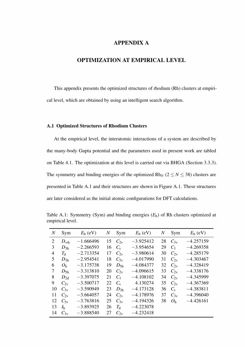
APPENDIX A

OPTIMIZATION AT EMPIRICAL LEVEL

This appendix presents the optimized structures of rhodium (Rh) clusters at empiri-

cal level, which are obtained by using an intelligent search algorithm.

A.1 Optimized Structures of Rhodium Clusters

At the empirical level, the interatomic interactions of a system are described by

the many-body Gupta potential and the parameters used in present work are tabled

on Table 4.1. The optimization at this level is carried out via BHGA (Section 3.3.3).

The symmetry and binding energies of the optimized RhN (2 ≤ N ≤ 38) clusters are

presented in Table A.1 and their structures are shown in Figure A.1. These structures

are later considered as the initial atomic configurations for DFT calculations.

Table A.1: Symmetry (Sym) and binding energies (Eb) of Rh clusters optimized atempirical level.

N Sym Eb (eV) N Sym Eb (eV) N Sym Eb (eV)

2 D∞h −1.666496 15 C2v −3.925412 28 C3v −4.2571593 D3h −2.266593 16 Cs −3.954654 29 C1 −4.2693584 Td −2.713354 17 C2v −3.980614 30 C2v −4.2851795 D3h −2.954541 18 C5v −4.017990 31 C2v −4.3034676 Oh −3.175738 19 D5h −4.084377 32 C2v −4.3284197 D5h −3.313810 20 C2v −4.096615 33 C2v −4.3381768 D2d −3.397075 21 C1 −4.108102 34 C2v −4.3459999 C2v −3.500717 22 Cs 4.130274 35 C2v −4.36736910 C3v −3.590949 23 D3h −4.173128 36 Cs −4.38381111 C2v −3.664057 24 C2v −4.178976 37 C3v −4.39604012 C5v −3.763816 25 C3v −4.194326 38 Oh −4.42616113 Ih −3.893925 26 Td −4.22307814 C3v −3.888540 27 C2v −4.232418

(i) Rh3 (ii) Rh4 (iii) Rh5 (iv) Rh6

(v) Rh7 (vi) Rh8 (vii) Rh9 (viii) Rh10

(ix) Rh11 (x) Rh12 (xi) Rh13 (xii) Rh14

(xiii) Rh15 (xiv) Rh16 (xv) Rh17 (xvi) Rh18

(xvii) Rh19 (xviii) Rh20 (xix) Rh21 (xx) Rh22

Figure A.1: Optimized structures of Rh clusters at empirical level.

127

(xxi) Rh23 (xxii) Rh24 (xxiii) Rh25 (xxiv) Rh26

(xxv) Rh27 (xxvi) Rh28 (xxvii) Rh29 (xxviii) Rh30

(xxix) Rh31 (xxx) Rh32 (xxxi) Rh33 (xxxii) Rh34

(xxxiii) Rh35 (xxxiv) Rh36 (xxxv) Rh37 (xxxvi) Rh38

Figure A.1: Optimized structures of Rh clusters at empirical level.

128

APPENDIX B

VIBRATIONAL FREQUENCY ANALYSIS

This appendix presents the zero-point energies and infrared spectra of optimized

rhodium (Rh) clusters from DFT calculations.

B.1 Zero-point Energy

Besides determining the nature of a stationary point, vibrational frequency analysis

provides the zero-point energy of the point. The zero-point energies of optimized Rh

clusters obtained from the present calculations are presented in Table B.1.

Table B.1: Zero-point energies of Rh clusters. The isomers of Rh4, Rh6 and Rh22clusters are labelled as (a) and (b).

NZero-point Energy

NZero-point Energy

NZero-point Energy

(kcal/mol) (kcal/mol) (kcal/mol)

2 0.4 10 4.8 20 11.23 0.9 11 5.8 21 11.84 (a) 1.8 12 5.7 22 (a) 12.64 (b) 2.8 13 7.1 22 (b) 12.45 2.1 14 7.3 23 13.26 (a) 3.2 15 8.2 26 14.76 (b) 2.8 16 8.6 30 17.17 3.4 17 9.5 38 22.98 3.9 18 9.99 4.9 19 10.5

B.2 Infrared Spectra

Also, the frequency analysis provides frequencies and intensities on all mode of

vibrations. These are then allowed one to plot the infrared spectrum of a stationary

point. Infrared spectra of Rh clusters, which have been geometrically relaxed at DFT

framework, are displayed in Figure B.1.

(i) Rh3 (ii) Rh4 (a)

(iii) Rh4 (b) (iv) Rh5

(v) Rh6 (a) (vi) Rh6 (b)

Figure B.1: Infrared spectra of Rh clusters.

130

(vii) Rh7 (viii) Rh8

(ix) Rh9 (x) Rh10

(xi) Rh11 (xii) Rh12

(xiii) Rh13 (xiv) Rh14

Figure B.1: Infrared spectra of Rh clusters.

131

(xv) Rh15 (xvi) Rh16

(xvii) Rh17 (xviii) Rh18

(xix) Rh19 (xx) Rh20

(xxi) Rh21 (xxii) Rh22 (a)

Figure B.1: Infrared spectra of Rh clusters.

132

(xxiii) Rh22 (b) (xxiv) Rh23

(xxv) Rh26 (xxvi) Rh30

(xxvii) Rh38

Figure B.1: Infrared spectra of Rh clusters.

133