studies on the initiation, propagation, and extinction of
TRANSCRIPT
Studies on the Initiation, Propagation, and Extinction
of Premixed Flames
Zheng Chen
A DISSERTATION PRESENTED TO THE FACULTY OF
PRINCETON UNIVERSITY
IN CANDIDACY FOR THE DEGREE OF
DOCTOR OF PHILOSOPHY
RECOMMENDED FOR ACCEPTANCE
BY THE DEPARTMENT OF
MECHANICAL AND AEROSPACE ENGINEERING
Advisor: Yiguang Ju
January, 2009

To My Parents and Advisors

© Copyright by Zheng Chen, 2009.
All rights reserved.

Abstract
Premixed flames are widely utilized in spark ignition engines for automobiles and
in advanced gas turbine engine systems for power generation. In the present study, the
fundamental properties of premixed flames such as initiation, propagation, and extinction
are systematically investigated using asymptotic theoretical analysis, detailed numerical
simulations, and/or experimental measurements.
A general theory on spherical flame initiation and propagation and an accurate
numerical algorithm for adaptive simulation of unsteady reactive flow are first developed.
The general theory describes different flame regimes and transitions among them. This
could be utilized to study effects of radiative heat loss, ignition power, and preferential
diffusion on spherical flame initiation, propagation, and extinction. The numerical solver
is thoroughly tested and validated. It is shown to be able to accurately and efficiently
model propagating flames with detailed chemical mechanisms.
With the help of the general theory and the numerical solver, the controlling
factor for spherical flame initiation and how it relates to the minimum ignition energy are
then investigated. It is found that there exists a critical flame radius controlling the
spherical flame initiation and that the minimum ignition energy is proportional to the
cube of the critical flame radius. Moreover, results show that the preferential diffusion
between heat and mass (Lewis number) plays an important role in the spherical flame
initiation. Both the critical flame radius and the minimum ignition energy are found to
increase with the Lewis number.
The general theory and the numerical solver are also employed to study the
accuracy of laminar flame speed measurements utilizing propagating spherical flames.
iii
Different effects such as ignition, unsteadiness, compression, and stretch are found to
decrease the accuracy of these measurements. New flame speed determination methods to
obtain more accurate flame speeds by correcting for these effects are developed. For
example, both the Compression-Corrected Flame Speed (CCFS) and the
Stretch-Corrected Flame Speed (SCFS) are demonstrated not only to significantly
improve the accuracy of the flame speed measurements but also to greatly extend the
parameter range of experimental conditions.
The effects of radiation on flame propagation, extinction, and flammability limits
are also investigated. Opposite trends for the change of flame propagation speed and
flame extinction/flammability limits are found for the outwardly and inwardly
propagating spherical fames. A functional expression for the Markstein length is found in
terms of the Lewis number and the radiative heat loss. Moreover, the spectrally
dependent radiation absorption effect on propagating spherical flames is measured by
using CO2-diluted CH4/O2/He mixtures at normal and elevated pressures. Radiation
absorption is found to increase the flame speed and extend the flammability limit. In
addition, the combined effects of flame curvature, radiation, and stretch on flame
extinction are revealed via premixed tubular flames. It is found that the coupling between
radiation and flame curvature leads to multiple flame bifurcations and extinction limits.
Finally, the effects of kinetic and transport coupling on ignition and flame
propagation are investigated by using dimethyl ether (DME) blended methane/air
mixtures. It is shown that the addition of a small amount of DME to methane leads to a
significant decrease in the ignition time, while the flame speed of DME/CH4/air mixture
is only linearly proportional to the DME fraction.
iv

Acknowledgements
Many people contributed, in different ways, to the realization of the research work
that resulted in this thesis.
First and foremost, I would like to express my most sincere gratitude to my
advisor, Professor Yiguang Ju, for his invaluable support, guidance, and encouragement
through my graduate study at Princeton. Professor Ju is the greatest mentor and it is my
great fortune to have him as my academic advisor. I am immensely grateful that he has
taken every step possible to nurture my personal as well as professional growth, and to
help me develop my career in an academia position. I am also grateful to Mrs. Limei Zhu.
On holidays she often threw a party chaired by Professor Ju in their house. The parties I
attended in these years gave me warmness as well as delicious Chinese food.
I thank Professor Chung K. Law and Professor Frederick L. Dryer for their
service on my doctoral committee and for their help on my study and research. The
outstanding teaching and continuous encouragement from Professor Law are greatly
appreciated. The inspiring discussions with Professor Dryer during lunch-time are also
greatly appreciated. Thanks also go to Professor Chung K. Law and Professor Paul D.
Ronney for reading my thesis and providing many helpful feedbacks which have greatly
improved the final form of this dissertation and to Professor Alexander Smits and
Professor Luigi Martinelli for taking the time to be my examiner.
I wish to acknowledge my colleagues and collaborators: Dr. Xiao Qin and Mr.
Michael Burke for collaborations on spherical flames; Dr. Xiaolong Gou and Mr.
Wenting Sun for collaborations on multi-scale modeling and mechanism reduction; Dr.
Zhenwei Zhao, Dr. Marcos Chaos, and Professor Frederick L. Dryer for collaborations on
v
studying dimethyl ether/methane dual-fuel; Dr. Genyuan Li and Professor Herschel
Rabitz for collaborations on applications of the high dimensional model representation;
and Dr. Takeshi Yokomori for collaborations on tubular flames.
I would like also thank other colleagues of the Princeton combustion group: Yuan
Xue, Bo Xu, Timothy Ombrello, Sang-Hee Won, Wenjun Kong, Jingning Shan, Tianfeng
Lu, Hoi Dick Ng, Heyang Wang, Jiao Yuan, Juan Li, Peng Zhang, Wei Liu, Kenneth
Kroenlein, Mac Hass, and Kenichi Takita. I am grateful to them for their friendship and
for inspiring me during daily interactions. Besides, thanks also go to the MAE staff for
their excellent professional work and especially to Jessica O'Leary and Kelley Lynn
Garza for administrative help during my graduate study.
I wish to acknowledge my master-course advisor, Professor Zi-Niu Wu, and other
teachers at Tsinghua University. I would never be able to finish the current research work
without the fundamentals on mathematics, fluid mechanis, and thermal engineering I
learned at Tsinghua University.
Finally, it is with profound gratitude that I thank my parents, Jinya Chen and
Guiying Liu, and my sister, Mei Chen, for their love and support. It is my parents’ hard
work over the years that made it possible for me to attend college and graduate school.
This dissertation carries the number 3196-T in the records of the Department of
Mechanical and Aerospace Engineering.
vi
Table of Contents
Abstract............................................................................................................................. iii
Acknowledgements ............................................................................................................v
Table of Contents ............................................................................................................ vii
Chapter 1: Introduction ....................................................................................................1
1.1 Overview and Significance .....................................................................................1
1.2 Historical Perspectives............................................................................................2
1.2.1 Flame Initiation and Minimum Ignition Energy.......................................... 2
1.2.2 Flame Propagation and Laminar Flame Speed ............................................ 7
1.2.3 Flame Extinction and Flammability Limit................................................. 11
1.3 Motivation and Objectives....................................................................................14
1.4 Organization of the Dissertation ...........................................................................21
1.5 List of Publications ...............................................................................................23
Chapter 2: Theoretical Analysis on Spherical Flame Initiation and Propagation.....25
2.1 Mathematical Model .............................................................................................25
2.2 Theoretical Analysis..............................................................................................28
2.2.1 Analytical Solution without External Energy Addition ............................. 29
2.2.2 Validation in Limiting Cases...................................................................... 31
2.2.3 Effect of Radiative Heat Loss .................................................................... 34
2.2.4 Correlation among Different Flame Regimes............................................ 37
2.2.5 Effects of Ignition Energy.......................................................................... 40
2.3 Numerical Modeling of the Unsteady Effect ........................................................43
2.6 Conclusions...........................................................................................................46
Appendix: Solutions for Cylindrical Flames ..............................................................47
Chapter 3: Adaptive Simulation of Unsteady Reactive Flow (A-SURF) ....................61
3.1 Governing Equations for Unsteady Reactive Flows.............................................61
3.1.1 General Conservation Equations................................................................ 61
3.1.2 Transport and Chemistry Models............................................................... 63
vii

3.2 Numerical Methods...............................................................................................66
3.2.1 Fractional-step Procedure .......................................................................... 67
3.2.2 Finite Volume Method ............................................................................... 69
3.2.3 Locally Adaptive Mesh.............................................................................. 70
3.3 Validation and Examples.......................................................................................71
Chapter 4: Critical Flame Radius and Minimum Ignition Energy for Spherical
Flame Initiation................................................................................................................88
4.1 Theoretical Analysis..............................................................................................88
4.1.1 Analytical Solutions ................................................................................... 88
4.1.2 Results and Discussions............................................................................. 89
4.2 Numerical Validation ............................................................................................94
4.2.1 Numerical Specifications ........................................................................... 94
4.2.2 Results and Discussions............................................................................. 95
4.3 Conclusions...........................................................................................................98
Chapter 5: On the Determination of Laminar Flame Speed using Propagating
Spherical Flames ............................................................................................................108
5.1 Introduction.........................................................................................................108
5.2 Constant Pressure Method ..................................................................................111
5.2.1 Validity of the Linear Relationship between Flame Speed and Stretch... 114
5.2.2 Effects of Ignition and Unsteady Transition ............................................ 116
5.2.3 Effect of Compression ............................................................................. 121
5.3 Constant Volume Method....................................................................................128
5.3.1 Effect of Stretch Rate............................................................................... 130
5.4 Conclusions.........................................................................................................137
Chapter 6: Effect of Radiation on Flame Propagation and Extinction ....................155
6.1 Radiation Effect on Propagating Spherical Flames ............................................155
6.1.1 Introduction.............................................................................................. 155
6.1.2 Mathematical Model and Asymptotic Solutions...................................... 156
6.1.3 Results and Discussions........................................................................... 160
6.1.4 Summary.................................................................................................. 163
viii

6.2 Radiation Reabsorption Effect on Flame Speed and Flammability Limits ........164
6.2.1 Introduction.............................................................................................. 164
6.2.2 Experimental and Numerical Specifications............................................ 164
6.2.3 Results and Discussions........................................................................... 165
6.2.4 Summary.................................................................................................. 170
6.3 Radiation Effect on Premixed Counterflow and Tubular Flames .......................171
6.3.1 Introduction.............................................................................................. 171
6.3.2 Mathematical Model and Asymptotic Solutions...................................... 171
6.3.3 Results and Discussions........................................................................... 179
6.3.4 Summary.................................................................................................. 187
Chapter 7: Ignition and Burning Properties of DME/methane Mixtures ................202
7.1 Introduction.........................................................................................................202
7.2 Experimental/numerical Specifications and Kinetic Model Selection ...............202
7.3 Results and Discussions......................................................................................205
7.3.1 Ignition Enhancement by DME Addition ................................................ 205
7.3.2 Flame Speed and Burned Markstein Length of DME/CH4 Dual Fuel..... 209
7.4 Conclusions.........................................................................................................213
Chapter 8: Summary and Recommendations .............................................................221
8.1 Summary .............................................................................................................221
8.2 Recommendations for Future Work....................................................................225
References.......................................................................................................................228
ix

Chapter 1: Introduction
1.1 Overview and Significance
Combustion has had significant impact on our daily lives since the beginning of
human history. It is the primary means by which mankind produces power: about 85% of
the world’s energy comes from combustion of fossil fuels. Meanwhile, combustion is
also responsible for nearly all of the anthropogenic emission of nitrogen oxides (NOx),
carbon monoxide (CO), particulates (such as soot and aerosols), and other by-products
that are harmful to human health and the environment. In recent years, environmental
regulations throughout the world have been tightened for engine emissions. The emission
standards for both NOx and particulates have been tightened and more restrictive
measures will be implemented in the coming years. Meeting these requirements is
becoming increasingly difficult and developing high-efficiency, low-emission devices for
the conversion of fossil energy is currently a major research goal in combustion and
engine design communities. For example, radically new engine designs are the only hope
for meeting the near-zero NOx and particulate emission commitments proposed for
implementation by 2012.
To facilitate the exploration of radically new concepts for high-performance
engines, science-based predictive models for fundamental combustion processes such as
ignition, flame propagation, and flame extinction should be developed. For example,
ultra-lean combustion is currently one of the most promising concepts for substantial
reduction of emissions while maintaining high efficiency. Operating near the lean
flammability limit poses significant challenges such as flame blow-off, combustion
1
instabilities, auto-ignition, and flashback. In addition, the slowdown of combustion heat
release at near-limit conditions encourages the coupling between chemistry and transport.
Therefore, understanding and controlling near limit combustion are crucial for the
successful design of ultra-lean combustion gas turbines and burners.
This study is focused on the fundamental properties of premixed flames, which
are widely utilized in spark ignition engines for automobiles and in advanced gas turbine
engine systems for power generation. Using combined modeling and experimental
approaches, this thesis includes investigations on the ignition, propagation, and extinction
of premixed flames.
1.2 Historical Perspectives
1.2.1 Flame Initiation and Minimum Ignition Energy
Ignition is the process whereby a medium capable of reacting exothermically is
brought to a state of rapid combustion (Williams 1985). It is one of the most important
problems in combustion. Understanding of flame initiation is important not only for
fundamental combustion research but also for fire safety control and the development of
low emission gasoline and homogeneous charge compression ignition (HCCI) engines
and alternative fuels. Phenomenologically, ignition can be classified into two modes:
self-ignition and forced-ignition (Glassman 1996). Self-ignition, which is also called
auto-ignition or spontaneous ignition, is caused by chain branching or thermal feedback
in a homogeneous mixture without input of either an external source of thermal energy or
active radicals into the system. Unlike self-ignition, forced-ignition is a result of electrical
discharge (spark), heated surface, shock wave, or pilot flame, with the locally initiated
2

flame front subsequently reaching a self-propagating state where the ignition source can
be removed without extinguishing the combustion process.
For self-ignition, there are two different modes according to the mechanisms of
ignition. The first mode is chain self-ignition, in which the chain branching factor at a
given temperature and pressure exceeds a critical value (Glassman 1996). The second
mode is thermal self-ignition, in which the thermal energy release rate is greater than the
heat loss rate and the temperature consequently increases exponentially until a flame
appears (Glassman 1996). Theory on chain self-ignition was first developed by Semenov
(1935) and Hinshelwood (1940). The thermal self-ignition was first presented in
analytical form by Semenov (1935) and later in more exact form by Frank-Kamenetskii
(1955).
For forced-ignition, there are many means, among which the spark ignition is the
first and most prevalent form. Most practical combustion devices require combustion
events to be initiated at predetermined locations and times, and spark ignition is the
primary means of accomplishing this task (Ronney 1994). Successful spark ignition
depends on the amount of energy in the form of heat and/or radicals deposited into the
combustible mixture. If the energy is smaller than a so-called minimum ignition energy
(MIE), the resulting flame kernel decays rapidly because heat/radicals conducts/diffuse
away from the surface of the ignition kernel and the dissociated species recombine faster
than they are generated by the chain-branching reactions within the ignition kernel.
Comprehensive experiments on spark ignition of different hydrocarbon fuels were
conduced by Lewis and von Elbe and large amounts of experimental data on the MIE
were reported (Lewis and Von Elbe 1961). To explain their observations of the MIE for
3

different mixtures, Lewis and von Elbe (1961) postulated the first theory of spark
ignition. They proposed that the spark heated the surrounding mixture and ensured
continued flame propagation. The minimum size of this heated “spark kernel” was
dictated by the condition that heat transferred from its surface by conduction was
balanced by heat generated by combustion inside the kernel. If the kernel volume was too
small, the heat conduction rate was greater than the heat generation rate and the flame
kernel would be extinguished. The minimum spark kernel size was believed to be related
to the quenching distance which the authors had observed in their experiments (Lewis
and Von Elbe 1961). It was then postulated that the MIE, Emin, was the spark energy
necessary to heat a sphere of gas whose diameter was equal to the quenching distance, dq,
to the flame temperature, Tf, of the mixture
)()(6 0
3min TTCdE fpq −= ρπ (1.1)
Similarly, based on the thermal-diffusion theory considering the competition
between the reaction heat release and conductive heat loss, Zeldovich (Zeldovich et al.
1985) proposed that the minimal ignition kernel radius for successful spherical flame
initiation was related to the laminar premixed flame thickness, δf0, and the MIE was
proportional to the cube of the flame thickness
)()(3
40
30min TTCE fpf −= ρδπ (1.2)
Unfortunately, the above models could only phenomenologically describe the
spark ignition since the fuel consumption and thus mass diffusion were not considered.
More accurate description of flame ignition including the effect of preferential diffusion
of heat and mass (Lewis number effect) was proposed later based on the studies about
4
flame balls (Deshaies and Joulin 1984; Zeldovich et al. 1985; Champion et al. 1986).
Zel’dovich (Zeldovich et al. 1985) found that for any premixed mixture there could exist
a diffusion controlled stationary flame ball with a characteristic equilibrium radius – the
flame ball radius. A stability analysis (Deshaies and Joulin 1984) showed that adiabatic
flame balls were inherently unstable: a small perturbation would cause the flame to
propagate either inward and eventually extinguish, or outward and evolve into a planar
flame. The unstable equilibrium flame ball radius was therefore considered to be a critical
parameter in controlling flame initiation and the MIE was proposed to be proportional to
the cube of the flame ball radius instead of the flame thickness (Zeldovich et al. 1985;
Champion et al. 1986). Since the flame ball radius strongly depends on the Lewis number
(Zeldovich et al. 1985), the MIE for mixtures with different Lewis numbers is totally
different. This was confirmed by numerical simulation using a one-step chemical
mechanism (Tromans and Furzeland 1988). Recently, He (2000) studied mixtures with
larger Lewis numbers and found that propagating spherical flames with radius less than
the flame ball radius could exist when the Lewis number was larger than a critical value.
Therefore, it was concluded that flame initiation for mixtures with large Lewis numbers
was not controlled by the radius of stationary flame ball (He 2000). All the above
theoretical studies were based on the quasi-steady assumption, neglecting the
unsteadiness of flame initiation. Using large activation energy asymptotic analysis, Joulin
(1985) studied the dynamics of flame kernels whose evolution was triggered by a
time-dependent point-source of energy and a parameter-free flame front evolution
equation for mixtures with Lewis numbers smaller than and bounded away from unity
was obtained.
5

While the simplified models (such as one-step chemistry, constant thermal
properties, quasi-steadiness, energy deposition as a boundary condition independent of
time and space) considered in the above theoretical studies are adequate to describe many
important qualitative features of the ignition process, they do not appear to be adequate
for quantitative accuracy (Ronney 1994). To include more quantitatively accurate and
perhaps even more qualitatively realistic models, numerical simulations were employed
to study the ignition process. Maas and Warnatz (1988) simulated the ignition process in
hydrogen/air mixtures by solving the corresponding conservation equations (total mass,
momentum, energy, and species mass) for one-dimensional geometries using a detailed
reaction mechanism and a multi-species transport model. Sloane and Ronney (1993)
compared the MIE for a stoichiometric methane/air mixture using a one-step chemical
mechanism and a detailed mechanism, and found that the differences in chemical
mechanisms had a substantial effect on the MIE. Other effects such as composition, size
of ignition source, duration of energy deposition, method of energy deposition, and flow
environment on the MIE were also investigated via numerical simulations, which were
reviewed by Ronney (1994). Spherical symmetry was usually assumed and
one-dimensional simulations of flame initiation were conducted for simplicity. To
provide a better understanding of the spark discharge process, two-dimensional
simulations were recently carried out and more sophisticated models including ionization
were employed (Akram 1996; Thiele et al. 2000; Thiele et al. 2002; Ekici et al. 2007).
Despite the extensive research on the flame initiation over many decades, the
determination of MIE still remains empirical and could not be predicted even
qualitatively by theory. To get a better understanding of the flame initiation and more
6

accurate prediction of the MIE, flame propagation after spark ignition should be studied
since successful ignition critically depends on whether the expanding flame kernel would
be able to maintain its propagation to reach a self-propagating state.
1.2.2 Flame Propagation and Laminar Flame Speed
When a sufficient amount of energy is locally deposited into a quiescent
homogeneous combustible mixture, a sustainable combustion wave can be initiated. For
some specific conditions of strong ignition, the combustion wave takes the form of a
detonation characterized by the supersonic propagation speed in the fresh mixture. The
detonation has a propagating shock front which is coupled with and sustained by
chemical heat release behind it (Williams 1985). For mild ignition, deflagrations (called
premixed flames in the following) can be initiated. In this study, the focus will be on
these premixed flames which propagate with a subsonic speed into the chemically-frozen,
fresh mixture.
The thickness of premixed flames is usually much smaller than the characteristic
length of the gas flow. Therefore, the flame front can be considered as a hydrodynamic
discontinuity between two non-reactive flows, the fresh mixture and the burnt gases, both
at thermo-chemical equilibrium (Clavin 1994). The motion of the flame front is
controlled not only by its inner structure where diffusion and chemical reaction dominate,
but also by the outer flow around it. Due to the coupling between diffusion and
hydrodynamics, the dynamics and structure of premixed flames cannot be described
completely by ordinary diffusion-reaction equations and thus are difficult to be analyzed
theoretically. Therefore, either only hydrodynamics or only diffusion was considered in
most of the previous studies. In the pioneering studies by Darrieus (1938) and Landau
7

(1944), the first stability analysis of a flame front was conducted and hydrodynamic
instability, induced by the thermal expansion across the flame front, was found to be the
main cause of the formation of cellular patterns on the flame front. The diffusive
processes inside the flame front were completely neglected in their studies. On the other
hand, other studies (Sivashinsky 1977; Joulin and Clavin 1979) deliberately neglected the
hydrodynamic effect by using the thermal-diffusive model in which the density was
assumed to be constant and the flame reduced to a simpler reaction-diffusion problem.
Extensive studies on the reaction-diffusion problem using asymptotic methods and
multiscale analyses were conducted, which were reviewed in the monograph by
Buckmaster and Lundford (1982).
The first study on the coupling of diffusion and hydrodynamics was carried out by
Markstein (1951). Based on semi-phenomenological considerations, the following
correlation between the local flame speed, Su, and the mean flame radius of curvature, R,
was proposed (Markstein 1951)
RLSS uuu /1/ 0 += (1.3)
where Su0 is the laminar flame speed of an adiabatic freely-propagating planar flame and
Lu is a length called the “Markstein length”. Lu depends on the diffusive properties of the
reactive mixture and has the same order in magnitude as the flame thickness, δf0. Later,
the curvature of the flow (defined as the divergence of the unit flow velocity taken just
upstream of the flame front) was included (Markstein 1964)
])/(/1[1/ 0−⋅∇++= uuRLSS uuu
vvv (1.4)
Another point of view was developed in a different context by Karlovitz
(Karlovitz et al. 1953) who introduced the concept of “flame stretch” and proposed that
8

the local flame speed, Su, was affected by the flame stretch. The flame stretch, K, was
defined as K=A-1dA/dt, where A is the elemental area of the flame front. It was shown
that flame stretch was contributed by two sources: flame curvature and flow
non-uniformity (Buckmaster 1982; Matalon 1983). For a weekly stretched flame, the
following linear relationship was obtained (Clavin and Williams 1982)
KLSS uuu −= 1/ 0 (1.5)
For an outwardly propagating spherical flame resulted from central spark ignition
in a quiescent homogeneous combustible mixture, the flame stretch is well defined as
(Lewis and Von Elbe 1961)
dtdR
RdtdA
AK f
f
21== (1.6)
where A=4πRf2 is the surface area of the flame front and Rf is the flame radius. When the
flame size is small, for example on the order of flame thickness, the propagating spherical
flame is strongly stretched according to the definition given by equation (1.6) and
therefore the flame speed is significantly affected by the flame stretch (Clavin 1985). To
achieve successful ignition, the MIE must be able to support the flame kernel to survive
the strong flame stretch and propagate out to reach a self-propagating state.
Extensively studies using asymptotic techniques were carried out to investigate
the propagating spherical flames. Ronney and Sivashinsky (Ronney and Sivashinsky
1989) studied the expanding spherical flame within the framework of a slowly varying
flame (SVF) theory. While reasonable predictions for Lewis number (Le) less than unity
were obtained, the results of the SVF theory were found to be physically unrealistic for
Le>1. Bechtold and co-workers (Bechtold and Matalon 1987; Addabbo et al. 2003;
9
Bechtold et al. 2005) investigated the hydrodynamic and thermal-diffusion instabilities
and effects of radiative loss in self-extinguishing and self-wrinkling spherical flames.
Frankel and Sivashinsky (1983, 1984) examined the thermal expansion effect in
propagating spherical flames in the limit of Le→1. Chung and Law (Chung and Law
1988) conducted integral analysis for propagating spherical flames for Le=1. All the
above studies were based on the assumption of large normalized flame radius
(Rf/δf0>>1). The recent work by He (2000) and Chen and Ju (2007) spanned all the
spherical flame sizes and transitions between flames at small and large radii.
One of the most important applications of propagating spherical flames in
fundamental combustion research is for laminar flame speed measurements. Recently, the
propagating spherical flames have been popularly utilized to measure the laminar flame
speed, Su0. The laminar flame speed, defined as the speed relative to the unburned gas
with which a planar one-dimensional flame front travels along the normal to its surface
(Andrews and Bradley 1972), is one of the most important parameters of a combustible
mixture. On the practical level, it affects the fuel burning rate in internal combustion
engines and the engine’s performance and emissions (Metghalchi and Keck 1980). On a
more fundamental level, it is an important target for the validation of kinetic mechanisms
(Law et al. 2003). In the last fifty years, substantial attention has been given to the
development of new techniques and the improvement of existing methodologies for
experimental determination of the laminar flame speed. Various experimental
approaches, reviewed in (Andrews and Bradley 1972; Rallis and Garforth 1980), have
been developed to measure the laminar flame speed utilizing different flame
configurations, including the outwardly propagating spherical flame (Lewis and Von
10

Elbe 1961; Bradley and Mitcheson 1976; Metghalchi and Keck 1980; Rallis and Garforth
1980; Hill and Hung 1988; Taylor 1991; Kwon et al. 1992; Aung et al. 1997; Bradley et
al. 1998; Tse et al. 2000), counterflow or stagnation flame (Tsuji 1982; Egolfopoulos et
al. 1989; Wu et al. 1999; Huang et al. 2004), Bunsen flame (Lewis and Von Elbe 1961),
and burner stabilized flat flame (Levy and Weinberg 1959; Van maaren et al. 1994). Due
to the lack of uniformity of the flame speed over the flame surface in the Bunsen flame
and the wall effects in the flat flame, the propagating spherical flame and the stationary
counterflow flame are among the most successful systems for flame speed measurements
(Rallis and Garforth 1980; Tse et al. 2000). However, due to the Reynolds number limit,
the counterflow flame method is difficult to apply at high pressures (e.g. above 10
atm)(Tse et al. 2000). Consequently, tracking the evolution of an outwardly propagating
spherical flame in a confined bomb is the most favourable method for measuring the
flame speed, especially at pressure above 10 atmosphere (Metghalchi and Keck 1980;
Bradley et al. 1998; Tse et al. 2000). This method will be investigated and utilized in the
present study.
1.2.3 Flame Extinction and Flammability Limit
For ultra-lean combustion utilized in high-efficiency low-emission engines such
as the HCCI, flame extinction is one of the most important problems on engine
performance. A fundamental understanding of flame extinction is therefore essential for
developing radically new engines.
Flame extinction usually occurs for near-limit mixtures and it could be caused by
different effects such as radiative heat loss, flame stretch, and flame curvature (Ju et al.
2001). It is well known that radiation heat transfer is a dominant mechanism for
11
near-limit flame extinction. Indeed the flammability limit is determined by the radiative
heat loss for unstretched premixed planar flames (Spalding 1957; Buckmaster 1976). For
non-adiabatic planar flames, the following relationship between the normalized flame
speed, U, and the normalized heat loss (which strongly depends on the fuel
concentration), L, was derived (Spalding 1957; Buckmaster 1976)
0)ln( 22 =+ LUU (1.7)
According to the above relationship, the flammability limit is defined by and
. For each combustible mixture above the flammability limit, i.e. L<L
eL /1* =
2/1* −= eU *=1/e,
there exist two laminar flame speed solutions and only the higher one is stable and thus
could be observed in experiments (Joulin and Clavin 1979).
The above theory works only for planar flames which are unstretched. For
stretched flames, the flammability limit can be modified by the combined effects of
thermal radiation and flame stretch. The effects of radiation and stretch were extensively
studied by using the counterflow flames (Sohrab and Law 1984; Maruta et al. 1996; Sung
and Law 1996; Buckmaster 1997; Ju et al. 1997; Ju et al. 1999a; Ju et al. 2000). These
studies showed that the flammability limit of stretched flames below a critical Lewis
number can be lower than that of unstretched flames. The extended flammable region
was found due to the existence of the Near Stagnation plane Flame (NSF) and the
flammability of the stretched flame below the critical Lewis number is characterized by
the limit of the NSF (Ju et al. 1999a). It was shown that the flammable region of
premixed counterflow flames was bounded by the stretch extinction limit at large stretch
rate and the radiation extinction limit at low stretch rate. Multi-flame bifurcations were
found theoretically (Buckmaster 1997) and numerically (Ju et al. 1997; Ju et al. 1999a) to
12
be intrinsic phenomena caused by the combined effects of radiation and flame stretch,
and the limits of these flame regimes were shown to be sensitive to the Lewis numbers of
reactants and to radiative heat losses.
Unlike the counterflow flames, practical flames such as the laminar propagating
spherical flames used in experiments and the flamelets in turbulent flames are not only
stretched but also curved. To include the curvature effect, the tubular flames (Ishizuka
1993; Ju et al. 1999b) and propagating spherical flames (Bechtold et al. 2005; Chen and
Ju 2007) have been utilized to study the combined effects of flame radiation, stretch, and
curvature on premixed flames. It has been shown that the interaction of flame curvature
with radiation or stretch greatly affects the flame strength and extinction.
In most of the studies mentioned above, radiation was only considered as heat loss
from the combustion system. However, radiation emission and reabsorption occur
simultaneously in combustion, and radiation from the downstream hot products could be
reabsorbed by the upstream cold mixture. The effect of radiation absorption on the flame
speed was first analyzed by Joulin and Deshaies (1986) using a gray gas model. It was
shown that there was no flammability limit when radiation absorption is considered. The
gray gas model was also used to study flame ball dynamics (Lozinski et al. 1994).
However, radiation of most species is not gray. For example, CO2 radiation is strongly
spectral dependent and has temperature and pressure broadening. Ju et al. (Guo et al.
1998; Ju et al. 1998) first used the non-gray statistical narrow band (SNB) model to study
CO2-diluted propagating flames and showed that a “fundamental” flammability limit
exists because of the emission-absorption spectra difference between the reactants and
products and band broadening. This model was later used in flame balls (Wu et al. 1999)
13

and high-pressure planar flames (Ruan et al. 2001). All these studies showed that
radiation absorption plays an important role in flame extinction and flammability limits
for CO2-diluted mixtures.
1.3 Motivation and Objectives
Flame initiation, propagation, and extinction are intriguing combustion
phenomena that also have substantial practical applications and deserve further research.
The motivation and objectives of the present study are listed below:
(1) When an external energy is locally deposited into a combustible mixture, there
are four possible outcomes: evolution from the outwardly propagating spherical flame to
a planar flame, a stationary flame ball, a propagating self-extinguishing flame, or a
decaying ignition kernel (Ronney 1988; He and Law 1999; Ju et al. 2001). The planar
flame, flame ball, and self-extinguishing flame have been extensively studied (Spalding
1957; Deshaies and Joulin 1984; Zeldovich et al. 1985; Ronney 1988; Buckmaster et al.
1990; Ronney 1990; Clavin 1994). However, previous studies only focused on the
dynamics of the separate phenomena such as flame balls and self-extinguishing flames,
and thus the propagating flames were isolated from flame balls and self-extinguishing
flames. As a result, the relation between self-extinguishing flames and flame balls and the
relation between the flame ball size and successful initiation of outwardly propagating
flames were not well understood. Recognizing the importance of the missing relationship
between flame balls and propagating flames, a theoretical analysis by He and Law (He
and Law 1999) was conducted to examine the transition of a flame ball to a propagating
spherical flame. Although it was concluded that radiative heat loss has a significant effect
on flame transition, the impact of radiative heat loss in the unburned region was not
14
considered. A recent study by He (2000) was motivated to study the flame initiation at
large Lewis numbers, but it did not consider radiative heat loss either. This makes the
results less realistic because near-limit flame initiation is dominantly affected by radiative
heat loss. Therefore, the role of heat loss on flame transition and the correlation among
the flame regimes from ignition kernels to flame balls and propagating flames remain
unknown.
In view of the above considerations, the first objective is to develop a general
theory which could describe the flame regimes and transitions among the flame kernel,
the flame ball, the self-extinguishing flame, the outwardly propagating spherical flame,
and the propagating planar flame, and to investigate the effects of radiative heat loss,
ignition energy, and preferential diffusion between heat and mass (Lewis number) on
flame transitions based on the general theory.
(2) As mentioned before, theoretical models usually only give qualitative rather
than quantitative predictions due to the simplify assumptions employed. For example, for
outwardly propagating spherical flames, it is unrealistic to obtain the flame propagation
speed as a function of flame radius predicted by theory to agree well with experimental
measurements because the theory is usually based on the assumption of one-step
irreversible chemical reaction with large activation energy. In order to get quantitative
results which could be utilized to compare with the experimental data, numerical
simulations including detailed chemical kinetics and accurate transport properties need to
be conducted. Besides, numerical simulation has many other advantages that make it an
attractive tool for scientific research and engineering design. For example, computer
simulations allow the user to interrogate the flow domain at any point in a non-intrusive
15

manner. Thus, filed information such as pressure, temperature, velocity, and species
concentration could be obtained without altering the flow field. Moreover, numerical
simulation also enables the user to separate the various processes that occur in a flow and
study the many complex interactions of these processes. For example, the role of
radiation on flame initiation and propagation may be better understood by studying cases
without radiation and then introducing radiation to isolate and thereby identify the
radiation effect on flame initiation and propagation. It would be exceptionally difficult, or
impossible, to accomplish this decoupling and removal of processes in experiments.
Therefore, the second objective is to develop a time-accurate and space-adaptive
numerical solver for the adaptive simulation of unsteady reactive flow. High-fidelity
numerical simulations of flame initiation, propagation, and/or extinction will be carried
out to validate the theoretical models and/or to explain experimental measurements.
(3) Flame initiation plays an important role in the performance of combustion
engines and a fundamental understanding of ignition is essential for a better control of
fuel efficiency, exhaust emission, and idle stability of the engine operation. Despite
extensive research effort over many decades on the determination of the MIE, it remains
unclear as the length scale controlling the spherical flame initiation and how it is related
to the MIE. Quenching distance or flame thickness was first considered to be the
controlling length scale and the MIE was proposed to be proportional to the cube of the
quenching distance or flame thickness (Lewis and Von Elbe 1961; Zeldovich et al. 1985).
Later, the unstable flame ball radius was considered to be the controlling length scale for
flame initiation and the MIE was proposed to be proportional to the cube of the flame ball
radius instead of the flame thickness (Deshaies and Joulin 1984; Zeldovich et al. 1985;
16

Champion et al. 1986). A recent study (He 2000) showed that propagating spherical
flame with radius less than the flame ball radius could exist when the Lewis number is
larger than a critical value. It was concluded that flame initiation for mixtures with large
Lewis numbers was not controlled by the radius of the stationary flame ball (He 2000).
More recent experiments (Kelley et al. 2008) on hydrogen/air ignition at different
equivalence ratios and pressures showed that there was a critical flame radius for
spherical flame initiation and successful ignition depended on whether the initially
ignited flame kernel can attain this critical radius. However, the relation between the
critical flame radius and the MIE was not examined in those studies. Therefore, more
studies should be carried out to clarify what is the controlling length scale for spherical
flame initiation. Moreover, since the MIE is a very important parameter, the next
question needs to be answered is how the controlling length scale is related to the MIE.
The third object of this study is therefore to find the controlling length scale for
spherical flame initiation and to reveal its relationship with the MIE.
(4) Currently the propagating spherical flame is popularly utilized to measure the
laminar flame speed and many experiments on different fuels at different conditions have
been conducted. However, it was found that large discrepancies exist among flame speed
data obtained from measurements using spherical flames and counterflow flames (Farrell
et al. 2004). The reason for this discrepancy has yet to be explained. The accuracy and
the validity of the employed models for flame speed measurements over a certain
parameter range in the spherical flame methods still remain unclear due to the complexity
of flame stretch, flow compression, flame structure, chamber geometry, and thermal
radiation. For example, in the constant-pressure method using propagating spherical
17

flames, the stretched flame speed is first obtained from the flame front history Rf=Rf(t)
and then is linearly extrapolated to zero stretch rate to obtain the unstretched flame speed
(Taylor 1991; Tseng et al. 1993; Bradley et al. 1996). Flame speeds are commonly
extrapolated over ranges of flame radius data, [RfL, RfU]. The lower bound, RfL, is often
chosen to reduce the effects of initial spark ignition, flame curvature, and unsteadiness on
the flame propagation speed, and to make stretch rate small such that the linear
relationship between the stretched flame speed and stretch rate is satisfied (Taylor 1991;
Tseng et al. 1993; Bradley et al. 1996). The upper bound, RfU, is frequently chosen to
ensure that the pressure change is “small”. Historically, the choice of the data range has
been somewhat arbitrary — different researchers made different choices without giving
quantitative justification. To the authors’ knowledge, there is no quantitative study on
how the flame radii range, [RfL, RfU], affects the measured flame speed and how to choose
the proper RfL and RfU in the literature. Similarly, in the constant-volume method using
propagating spherical flames (Lewis and Von Elbe 1961; Metghalchi and Keck 1980;
Hill and Hung 1988), stretch effect on the laminar flame speed might be too large to be
neglected and thus the stretch correction for obtaining accurate unstretched laminar flame
speed is indispensable (Wu et al. 1999). However, in all previous studies using the
constant-volume method, the effect of flame stretch was neglected (Lewis and Von Elbe
1961; Metghalchi and Keck 1980; Hill and Hung 1988; Parsinejad et al. 2006). The
stretch effect for the constant-volume method addresses two concerns: how much does
the stretch affect the accuracy of flame speed measurement; and how does one correct the
stretch effect in the flame speed measurements.
18

The fourth objective is therefore to answer the questions posed above. Different
effects such as ignition and unsteady transition, compression, and flame stretch on the
accuracy of laminar flame speed measurements using propagating spherical flames will
be investigated and new methods to obtain more accurate flame speeds in a broader
experimental range by correcting for these effects will be developed.
(5) It is well known that curved flame fronts prevail in turbulent combustion and
the effect of curvature on flame propagation is important, especially for near-limit flames.
Therefore, in order to extend the flammability and to improve flame stability for ultra
lean combustion engines, it is particularly important to understand how the coupling of
thermal radiation, flame curvature, and flame stretch affects the flame speed and
extinction limits. Extensive studies have been conducted to investigate the effects of
radiation, stretch, and curvature on flame extinction by using the counterflow flames and
outwardly propagating spherical flames (Frankel and Sivashinsky 1984; Sohrab and Law
1984; Flaherty et al. 1985; Maruta et al. 1996; Sung and Law 1996; Buckmaster 1997; Ju
et al. 1997; Ju et al. 1999a; Ju et al. 2000; Bechtold et al. 2005; Chen and Ju 2007).
However only radiation together with stretch or stretch together with curvature was
considered and the combined effects of radiation with both stretch and curvature were not
addressed in all the previous studies except for the numerical study by Ju et al. (Ju et al.
1999b). Therefore, to gain a clear understanding of the extinction mechanism and to
obtain an explicit correlation of the flammability limit, it is necessary to perform an
analytical study to investigate the combined effects of radiation, stretch, and curvature on
flame propagation and extinction.
Furthermore, with the recent development of high pressure combustor for high
19

energy efficiency and low NOx and soot emission technology, a large amount of CO2 is
recycled to the unburned mixture. As such, the strong spectral radiation absorption of
CO2 and the appearance of large amount of CO2 in the recirculated exhausted gas raise
the following question: what is the role of CO2 radiation in flame speed and flammability
limit? This concern becomes more serious with increasing ambient pressure. In most of
previous studies, only radiative heat loss was considered. However, CO2 not only is a
radiation emitter but also an absorber. Therefore, it is important to know the effect of
radiation absorption due to CO2 on flame extinction and flammability limit.
Based on the above considerations, the fifth objective is to study the combined
effects of radiation, stretch, and curvature on flame propagation and extinction, and to
investigate the extension of flammability limits and the increase of laminar flame speeds
due to the spectral dependent radiation absorption.
(6) Dimethyl ether (DME) is emerging as a substitute for Liquefied Petroleum
Gas (LPG), diesel fuels, and Liquefied Natural Gas (LNG) because it has low soot
emission, no air or ground-water pollution effects, and can be mass produced from
natural gas, coal or biomass (Semelsberger et al. 2006; Arcounianis et al. 2008). Recently,
the study of DME combustion has received significant attention. DME has shown
promise as an additive and/or fuel extender. Yao et al. (2005) have undertaken studies on
DME addition to methane for homogeneous charge compression ignition (HCCI) engines.
In such cases, the coupling of DME kinetics with those of methane involves the low
temperature kinetics of DME. On the other hand, DME/methane utilization in burners
and in gas turbine applications is expected to involve principally high temperature kinetic
coupling effects. However, the underlying kinetic coupling between DME and CH4
20

responsible for the observed ignition enhancement was not explored in any detail. In
addition, kinetic coupling effects on flame properties and auto-ignition in non-premixed
systems have not been studied.
Moreover, it is well known that flame properties such as burning rate and flame
stability depend on the overall activation energy and the Lewis number or the Markstein
length (Clavin 1985; Law 2006). Kinetic coupling may result in a dramatic change in
the overall activation energy with a small amount of DME addition to methane.
Furthermore, DME has a molecular weight larger than air so that the Le is larger than
unity for lean DME/air mixtures in comparison to methane/air mixtures. On the other
hand, DME is expected to react more quickly in the preheating zone by decomposing to
lighter molecules. Therefore, it is of interest to investigate how the effective mixture
Lewis number or the Markstein length depends on the blending ratio of dual fuels with
disparate molecular weights, such as DME/CH4 mixtures.
Thus the sixth and last objective of the present study is to investigate the kinetic
coupling effects of DME addition on the high temperature ignition and burning properties
of methane/air mixtures.
The above motivation and objectives basically provide the guideline for the
dissertation research, with the following structure.
1.4 Organization of the Dissertation
Chapter 2 presents a general theory on spherical flame initiation, propagation, and
extinction. Based on this theory, the dynamics of flame kernel evolution with and without
ignition energy deposition is studied and the effects of radiative heat loss and Lewis
number on flame propagation are investigated.
21

Chapter 3 describes the numerical solver for Adaptive Simulation of Unsteady
Reactive Flow (A-SURF). The details on the governing equations, numerical methods,
and code validation for A-SURF are reported.
Chapter 4 is concerned with flame initiation. The critical flame radius and
minimum ignition energy for spherical flame initiation are studied. The emphasis is on
investigating the effect of preferential diffusion between heat and mass on the flame
kernel evolution and the minimum ignition energy.
Chapter 5 is focused on flame propagation. The constant pressure and constant
volume methods utilizing propagating spherical flames for laminar flame speed
measurements are investigated. New methods to obtain more accurate flame speed in a
broader experimental range are presented.
Chapter 6 is focused on flame extinction. Different effects such as radiative heat
loss, stretch, curvature, and preferential diffusion on flame extinction are identified. The
extension of flammability limits and the increase of laminar flame speeds due to the
spectral-dependent radiation reabsorption are also discussed.
Chapter 7 reports the ignition and burning properties of the dimethyl
ether/methane dual fuel. The effect of dimethyl ether addition to methane-air mixtures on
ignition, flame speed, and Markstein length is studied. New experimental data were
obtained for the validation of existing chemical mechanisms.
Chapter 8 summarizes the present theoretical analysis, numerical modeling, and
experimental work, and provides recommendations for future work.
22

1.5 List of Publications
Chapter 2: Z. Chen, Y. Ju, “Theoretical analysis of the evolution from ignition kernel to
flame ball and planar flame,” Combustion Theory and Modelling, 11 (2007)
427-453.
Chapter 4: Z. Chen, M.P. Burke, Y. Ju, “On the critical flame radius and minimum
ignition energy for spherical flame initiation,” In preparation, 2009.
Chapter 5: Z. Chen, M.P. Burke, Y. Ju, “Effects of Lewis number and ignition energy on
the determination of laminar flame speed using propagating spherical flames,”
Proceedings of the Combustion Institute, 32 (2009) In press.
Z. Chen, M.P. Burke, Y. Ju, “Effects of compression and stretch on the
determination of laminar flame speed using propagating spherical flames,”
Combustion Theory and Modelling, (2009) In press.
Chapter 6: Z. Chen, Y. Ju, “Combined effects of curvature, radiation, and stretch on the
propagation and extinction of spherical flames,” In preparation, 2009.
Z. Chen, X. Qin, B. Xu, Y. Ju, F. Liu, “Studies of radiation absorption on
flame speed and flammability limit of CO2 diluted methane flames at elevated
pressures,” Proceedings of the Combustion Institute, 31 (2007) 2693-2700.
Z. Chen, Y. Ju, “Combined effects of curvature, radiation, and stretch on the
extinction of premixed tubular flames,” International Journal of Heat and
Mass Transfer, 51 (2008) 6118-6125.
Chapter 7: Z. Chen, X. Qin, Y. Ju, Z. Zhao, M. Chaos, F.L. Dryer, “High temperature
ignition and combustion enhancement by dimethyl ether addition to
23
methane-air mixtures,” Proceedings of the Combustion Institute, 31 (2007)
1215-1222.
Note that the experimental work published in the papers related to Chapters 4 and 5 was
conducted by Mr. M.P. Burke and thus not presented in the dissertation. The
experimental work reported in Chapters 6 and 7 and their related papers was conducted
by the author with the help of Dr. X. Qin. The analysis on ignition presented in Chapter 7
and its related paper was carried out jointly with Drs. Z. Zhao, M. Chaos, and F.L. Dryer.
24

Chapter 2: Theoretical Analysis on Spherical Flame
Initiation and Propagation
In this chapter, a general theory on spherical flame initiation and propagation is
presented. The dynamics of flame kernel evolution with and without external energy
deposition is studied using large-activation-energy asymptotic analysis. The effects of
radiative heat loss, ignition energy, and Lewis number on the correlation and transition
among the initial flame kernel, the self-extinguishing flame, the flame ball, the outwardly
propagating spherical flame, and the propagating planar flame are investigated. The
theory will be utilized to study ignition and flame speed measurement in Chapter 4 and
Chapter 5, respectively.
2.1 Mathematical Model
We consider the evolution of an unsteady, one-dimensional spherical flame kernel
with and without an external energy source at the center. By assuming constant thermal
properties, the conservation equations for energy and fuel mass in a quiescent flow are
given as
ωλρ ~~~)~~~~(~~
1~~~~ 2
2 qHrTr
rrtTCP +−
∂∂
∂∂
=∂∂ (2.1a)
ωρρ ~)~~~~~(~~
1~~
~ 22 −
∂∂
∂∂
=∂∂
rYDr
rrtY (2.1b)
where t~ , r~ , ρ~ , T~ and Y~ are time, radial coordinate, density, temperature, and fuel
mass fraction, respectively. is the chemical heat release per unit mass of fuel, q~ PC~
the specific heat capacity at constant pressure, λ~ the thermal conductivity, and D~ the
25

fuel mass diffusivity. To further simplify the problem in theoretical analysis, we also
adopt the commonly used constant density assumption (Joulin and Clavin 1979) so that
the convection flux is absent. ω~ is the reaction rate for a one-step irreversible reaction,
)~~/~exp(~~~ 0TREYA −ρ , in which A~ is the pre-factor of Arrhenius law, E~ the activation
energy, and 0~R the universal gas constant. The volumetric radiative heat loss H~ is
estimated by using the optically thin model, )~~(~~4~ 44∞−= TTKH pσ , where σ~ is the
Stefan-Boltzmann constant and pK~ denotes the Planck mean absorption coefficient of
the mixture.
By using the adiabatic planar flame speed, 0~uS , and the flame thickness,
)~~~/(~~ 00uPf SCρλδ = , the flow velocity, length, time, temperature, and reactant (fuel) mass
fraction can be normalized as
0~~
LSuu = , 0~
~
f
rrδ
= , 00 ~/~
~
uf Stt
δ= ,
∞
∞
−−
=TT
TTTad
~~~~
, ∞
=YYY ~~
(2.2)
where ∞T~ and ∞Y~ denote the temperature and fuel mass fraction in the fresh mixture,
respectively, and Pad CqYTT ~/~~~~∞∞ += is the adiabatic flame temperature. By further
attaching the coordinate to the moving flame front, R=R(t), the non-dimensional
equations take the following form
ω+−∂∂
∂∂
=∂∂
−∂∂ H
rTr
rrrTU
tT )(1 2
2 (2.3a)
ω−∂∂
∂∂
=∂∂
−∂∂ −
)( 22
1
rYr
rrLe
rYU
tY (2.3b)
26

where DCLe P~~~/~ ρλ= is the Lewis number and dtdRU /= is the flame front
propagating speed. The radiative heat loss and chemical reaction rate are normalized,
respectively, as
)~~(~~~
~~
0
0
∞−=
TTSCH
HaduP
f
ρδ
, ∞
=YSu
f~~~
~~0
0
ρδω
ω (2.4)
One can see that the present model extends the previous theoretical flame ball
models (Zeldovich et al. 1985; Buckmaster et al. 1990; Buckmaster et al. 1991) by
including propagating flames and radiative heat loss in both the burned and unburned
zones. Therefore the correlation between flame ball and propagating flames and the
impact of radiation on the flame transition among different flame regimes can be
examined.
In the limit of large activation energy, chemical reaction occurs only within a very
thin zone of high temperature and the reaction rate can be replaced by a Delta function
with jump conditions used at the flame front (Sivashinsky 1977; Joulin and Clavin 1979;
Law 2006)
)()1(
12
exp RrT
TZ
f
f −⋅⎥⎥⎦
⎤
⎢⎢⎣
⎡
−+−
= δσσ
ω (2.5)
where adTREZ ~~/)1(~ 0σ−= is the Zel’dovich number and adTT ~/~∞=σ the expansion
ratio. By integrating the conservation equations (2.3a) and (2.3b) around the flame front
(r=R), the jump relations for temperature and fuel mass fraction can be obtained as
(Sivashinsky 1977; Joulin and Clavin 1979)
⎥⎥⎦
⎤
⎢⎢⎣
⎡
−+−
=−=−−++− f
f
RRRR TTZ
drdY
drdY
LedrdT
drdT
)1(1
2exp)(1
σσ (2.6)
27

In this study, we shall also examine the impact of external energy deposition on
the flame initiation and flame transition. A constant energy flux is locally deposited in an
initially homogeneous mixture. For an initial flame kernel with a radius of , the center
of the flame kernel is located at
R
0=r , and Rr ≤≤0 and ∞<≤ rR are respectively
the burned and unburned regions. By defining the flame as the location where the fuel
concentration goes to zero, the boundary conditions for temperature and fuel mass
fraction can be given as
0,/,0 2 =−=∂∂= YQrTrr (2.7a)
0,, === YTTRr f (2.7b)
1,0, ==∞= YTr (2.7c)
where is the normalized ignition power given by Q
)~~(~~4
~0
∞−=
TTQQ
adfδλπ (2.8)
2.2 Theoretical Analysis
The unsteady problem given by equations (2.3a, 2.3b) cannot be solved
analytically. In fact, as will be demonstrated later by numerical simulations, it is
reasonable to assume that in the attached coordinate moving with the flame front, the
flame can be considered as in quasi-steady state (∂/∂t=0). This assumption has also been
used in previous studies (Frankel and Sivashinsky 1983; Deshaies and Joulin 1984;
Frankel and Sivashinsky 1984; He 2000). Therefore, the governing equations can be
simplified to
ω+⋅−=− ThdrdTr
drd
rdrdTU )(1 2
2 (2.9a)
28

ω−=−−
)( 22
1
drdYr
drd
rLe
drdYU (2.9b)
In addition, for the convenience of the algebraic manipulation the heat loss term H
is approximated by a linear function of the normalized temperature as , where
is the heat loss constant taking the following form
ThH ⋅=
h
3200
440 ~)~~~(
~~~4)~~(~~~
)~~(~~~4ad
LP
p
LP
fp TSC
KTTSCTTK
hρ
λσρ
δσ≈
−−
=∞
∞ (2.10)
Note that the radiative heat loss constant involves the radiation intensity and the
fuel concentration. For any mixtures, a decrease of fuel concentration (decrease of flame
speed) means an increase of h. For methane-air flames, the heat loss constant, h,
calculated according to equation (2.10) is in the range of 0.001 to 0.05.
2.2.1 Analytical Solution without External Energy Addition
Equation (2.9) with boundary conditions given by equation (2.7) can be solved
analytically for Q=0. An exact solution of temperature and fuel mass fraction distribution
is presented below. For fuel lean cases, the fuel mass fraction in burned gas region
( ) is zero and that in unburned gas region (Rr ≤≤0 ∞<≤ rR ) is obtained by solving
equation (2.9b) with boundary conditions given by equations (2.7b, 2.7c)
RrfordederYR
ULe
r
ULe
≥−= ∫∫∞ −∞ −
ττ
ττ
ττ
22 /1)( (2.11)
As to the temperature distribution, for adiabatic flames (h=0), the analytical
solution is
⎪⎩
⎪⎨
⎧
≥
≤≤=
∫∫∞ −∞ −
R
U
r
U
f
f
RrfordedeT
RrforTrT
ττ
ττ
ττ
22 /
0)( (2.12)
29

For nonadiabatic flames, since the radiation properties in burned and unburned
gases may be different, we use and to represent the heat loss constants in the
burned and unburned regions, respectively. Therefore, the individual contribution of the
radiative heat loss from these two regions can be examined. By defining
1h 2h
)2 ,1(42 =+= ihUk ii , an analytical solution of the temperature distribution is
obtained as
[ ]
[ ]⎪⎪⎩
⎪⎪⎨
⎧
≥−−−−
⋅
≤≤−−
⋅=
−+
−+
RrforkUkURkGkUkUrkGeT
RrforkUkURkFkUkUrkFeT
rTrRkU
f
rRkUf
)/,/,()/,/,(
0)/,/,()/,/,(
)(
222
222))((5.0
111
111))((5.0
2
1
(2.13)
where and . ∫ −=1
0
)1(),,( dtttecbaF cbat ∫∞
+=0
)1(),,( dtttecbaG cbat
Note that this exact solution removes the assumption of small heat loss
( ) which is commonly employed in previous studies (Joulin and Clavin
1979; Buckmaster et al. 1990; Buckmaster et al. 1991). Therefore, the present study
provides a more rigorous consideration of radiation modelling to understand the relation
between spherical flames and the far field propagating planar flames in the limit of
.
1/1~ <<Zh
∞→R
By using the jump relations given by equation (2.6), one obtains the following
algebraic system of equations for the flame propagation speed, U, flame radius, R, and
flame temperature, Tf
⎥⎥⎦
⎤
⎢⎢⎣
⎡
−+−
==⋅Ω ∫∞
−−−−
f
f
R
ULeULeRf T
TZdeeRLe
T)1(
12
exp/1 22
σσττ τ (2.14a)
where
30
⎪⎪⎪⎪⎪
⎩
⎪⎪⎪⎪⎪
⎨
⎧
≠−−
−+−+
−−+
+−
≠=−−
−+−+
+
=≠+−
−++
+−
==
=Ω∫
∫∞
−−−−
∞−−−−
0)/,/,(
)/,/1,()/,/,(
)/,/1,(2
0,0)/,/,(
)/,/1,(2
0,0/)/,/,(
)/,/1,(2
0,0/
21222
2222
111
1111
12
21222
2222
2
2122
111
1111
1
2122
hhifkUkURkG
kUkURkGk
kUkURkFkUkURkF
kkk
hhifkUkURkG
kUkURkGk
kU
hhifdeeRkUkURkF
kUkURkFk
kU
hhifdeeR
R
UUR
R
UUR
ττ
ττ
τ
τ
(2.14b)
The present work extends the study of He (He 2000) by considering the coupling
of radiative heat loss with the flame kernel evolution, which is the key mechanism for
near-limit flames, and allows bridging between the spherical flame limits and the
flammability limit of planar flames. By solving equation (2.14) numerically, the relation
for the flame propagation speed, flame radius, and flame temperature and the existence of
different flame regimes at different radiative heat loss intensities (or different fuel
concentrations) and/or different Lewis numbers can be obtained.
2.2.2 Validation in Limiting Cases
In the following, it will be shown that in different limiting cases the present model
recovers the previous results of stationary flame balls (Buckmaster et al. 1990;
Buckmaster et al. 1991), outwardly propagating spherical flames (Frankel and
Sivashinsky 1984), and planar flames (Joulin and Clavin 1979).
2.2.2.1 Stationary Flame Balls
In previous studies (Buckmaster et al. 1990; Buckmaster et al. 1991), the
non-adiabatic stationary flame ball was investigated via asymptotic analysis under the
assumption of small heat loss ( Zhh in /1 = , ). The relation between heat loss
and flame radius was
22 / Zhh out=
31

⎟⎟⎠
⎞⎜⎜⎝
⎛+⎟⎟
⎠
⎞⎜⎜⎝
⎛=⎟⎟
⎠
⎞⎜⎜⎝
⎛
Zout
Zin
Z RRL
RRL
RR
2
ln (2.15)
where [ ]22
)1(6 fZ
fZZinin T
TRhLσσ −+
= and [ ]2)1(2 fZ
fZZoutout T
TRhL
σσ −+= fZT. and are
flame temperature and radius of adiabatic stationary flame ball (Zeldovich et al. 1985).
ZR
LeTfZ
1= , ⎥
⎦
⎤⎢⎣
⎡−−
−−⋅=
)1(11
2exp1
LeLeZ
LeRZ σ
(2.16)
In the present study, the exact solution for the fuel mass fraction and temperature
distribution is obtained without using the small heat loss assumption. In the limit of
for flame balls, equation (2.14) reduces to the following form for the nonadiabatic
stationary flame ball
0=U
⎥⎥⎦
⎤
⎢⎢⎣
⎡
−+
−=
⋅=+
f
fff T
TZLeRRh
hThT
)1(1
2exp1
)tanh( 1
12 σσ
(2.17)
If the small heat loss assumption ( Zhh in /1 = , ) is used and
high-order terms of are neglected, the above relation can be reduced to the same
form as equation (2.15). Therefore, the flame ball solution (Buckmaster et al. 1990;
Buckmaster et al. 1991) is a limiting case of the present result.
22 / Zhh out=
Z/1
2.2.2.2 Outwardly Propagating Spherical Flames
A flame speed relation for propagating spherical flames was obtained by Frankel
and Sivashinsky (1984). It is readily seen that the present result given by equation (2.14)
recovers the same result in the limit of zero heat loss and large flame radius ( 021 == hh
and ). Specifically, for , the exponential integral can be represented by an
asymptotic series
1>>R 1>>R
32

RULedeeR
R
ULeULeR 2/ 22 +≈∫∞
−−−− ττ τ (2.18)
By using the above expansion, equation (2.14) reduces to the following form
⎥⎥⎦
⎤
⎢⎢⎣
⎡
−+
−=+=+
f
ff T
TZRLe
UR
UT)1(
12
exp21)2(σσ
(2.19)
The following relation can be immediately derived from equation (2.19), which is
similar to the theory presented in (Frankel and Sivashinsky 1984)
)11(2)11()2ln()2( −−−=++LeRLeR
ZR
UR
U (2.20)
The only difference between equation (2.20) and the relation from Frenkel and
Sivashinsky (Frankel and Sivashinsky 1984) is the additional second term on the right
hand side of equation (2.20), which was not considered by Frenkel and Sivashinsky for
Z→∞ and Le→1. Since the Zel’dovich number for most mixtures is in the range of 5~15
such that the deviation of Lewis number from unity can be of order of unity, the second
term on the right hand side of equation (2.20) can not be neglected.
As such, the present model is valid in both limits of flame ball and propagating
flames and can provide the relationship and transition mechanism between these two
flames during the flame kernel growth.
2.2.2.3 Planar Flames
In the limit of , the functions and respectively become ∞→R F G
1)/,/,(
)/,/1,(
111
111 →−
−+kUkURkF
kUkURkF , 0)/,/,(
)/,/1,(
222
222 →−−
−+−kUkURkG
kUkURkG
Therefore, equation (2.14) reduces to
33
⎥⎥⎦
⎤
⎢⎢⎣
⎡
−+−
==+
f
ff T
TZUkkT)1(
12
exp2
21
σσ (2.21)
Asymptotically, when the heat loss is of the order of in the limit of large
Zel’dovich number ( ,
Z/1
Zhh in /1 = Zhh out /2 = , and 1>>Z ), equation (2.21) recovers
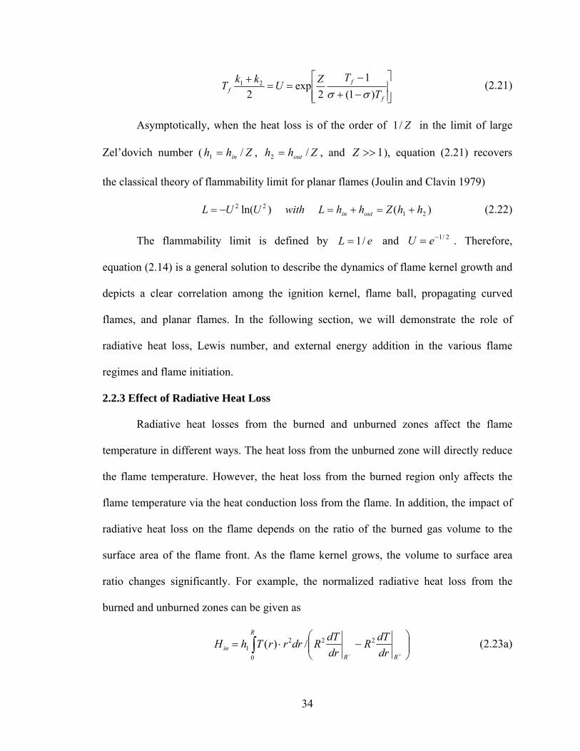
the classical theory of flammability limit for planar flames (Joulin and Clavin 1979)
)()ln( 2122 hhZhhLwithUUL outin +=+=−= (2.22)
The flammability limit is defined by eL /1= and . Therefore,
equation (2.14) is a general solution to describe the dynamics of flame kernel growth and
depicts a clear correlation among the ignition kernel, flame ball, propagating curved
flames, and planar flames. In the following section, we will demonstrate the role of
radiative heat loss, Lewis number, and external energy addition in the various flame
regimes and flame initiation.
2/1−= eU
2.2.3 Effect of Radiative Heat Loss
Radiative heat losses from the burned and unburned zones affect the flame
temperature in different ways. The heat loss from the unburned zone will directly reduce
the flame temperature. However, the heat loss from the burned region only affects the
flame temperature via the heat conduction loss from the flame. In addition, the impact of
radiative heat loss on the flame depends on the ratio of the burned gas volume to the
surface area of the flame front. As the flame kernel grows, the volume to surface area
ratio changes significantly. For example, the normalized radiative heat loss from the
burned and unburned zones can be given as
⎟⎟⎠
⎞⎜⎜⎝
⎛−⋅=
+−∫
RR
R
in drdTR
drdTRdrrrThH 22
0
21 /)( (2.23a)
34

⎟⎟⎠
⎞⎜⎜⎝
⎛−⋅=
+−∫∞
RRRout dr
dTRdrdTRdrrrThH 222
2 /)( (2.23b)
where ⎟⎟⎠
⎞⎜⎜⎝
⎛−
+− RR drdTR
drdTR 22 is the total heat generation from chemical reaction. By
using the temperature distribution obtained in equation (2.13), the ratio of the heat loss in
the limit of small and large flame radius becomes
⎪⎩
⎪⎨
⎧
∞→−+
++⋅
→
= RifUh
Uhhh
Rif
HH
out
in
1/41
1/4100
21
22
2
1 (2.24)
The above qualitative result shows that the radiative heat loss from burned and
unburned zones will have different impacts on the flame temperature and flame
transition. Since the radiative heat loss in the unburned region was neglected in the
previous theoretical studies (He and Law 1999; He 2000), the competing role of radiative
heat loss from the unburned and burned zones as the flame kernel grew was not
identified.
In the following we will take an example of CH4/air flames and use equation
(2.14) to demonstrate how differently the radiative heat losses from the burned and
unburned regions affect the flame temperature and flame propagation speed. For flames
around the stoichiometric equivalence ratio, we choose 10=Z and 15.0=σ . Equation
(2.23) is utilized to evaluate the radiative heat loss from different zones and the total
normalized radiative heat loss is their summation: Hall=Hin+Hout.
Figure 2.1 shows the dependence of normalized heat loss and flame propagation
speed on the flame radius for 1=Le and 015.0=h . It is seen that there are two flame
branches in the diagram: the fast stable flame branch abc and the slow unstable RU −
35

flame branch cde. At point c, the flame is extinguished at a finite propagating speed
because the normalized heat loss reaches its maximum on the fast flame branch abc. It is
also observed that the normalized total heat loss changes nonmonotonically as the flame
radius increases. There exists a minimum value as the flame reaches point b on the fast
branch and point d on the slow branch, respectively. This phenomenon can only be
explained by considering the individual contributions of heat loss in the burned and
unburned zones.
The dependence of the normalized radiative heat loss in the burned and unburned
zones, and , on flame radius are shown in figure 2.1(b). It is seen that
increases monotonically with flame radius while decreases monotonically with
flame radius. It is shown that the radiative heat loss from the unburned zone
remains nearly constant when the flame radius is larger than 20 and is an order smaller
than ( when ). This means that the effect of heat loss in the
unburned zone becomes weaker as the flame grows. However, it does not mean that heat
loss from the unburned zone can be neglected because the heat loss from these zones
affect the flame temperature in different ways. The rapid increase of flame speed and the
peak of the radiative heat loss in the region of
inH outH inH
outH
outH
inH 1.0/ <inout HH 20>R
20<R are caused by the competition of
radiative heat loss from the burned and unburned zones.
When the radiative loss is larger than the critical loss ( eL /1= and 0184.0=ch )
at the flammability of the planar flame, a flame does not exist at larger flame radii. Figure
2.2 shows the dependence of the normalized heat loss and flame propagation speed on the
flame radius for and 1=Le 0197.0=h . It is interesting to note that a propagating
spherical flame still exists at intermediate flame radii and has two extinction limits,
36
respectively, at small and large flame radii. The normalized total heat loss also changes
non-monotonically and peaks at both extinction limits. This indicates that the extinction
at small flame radius is caused by the heat loss in the unburned zone and the extinction at
large flame radius by that from the burned zone (figure 2.2b). The appearance of the
extinction limit at small flame radius has not been reported in previous studies and the
existence of this extinction limit will significantly affect the ignition kernel size for
successful flame initiation. Therefore, adequate inclusion of radiative loss from unburned
gas is particularly important for understanding the flame kernel evolution.
2.2.4 Correlation among Different Flame Regimes
Figure 2.3(a) shows the flame propagation speed as a function of flame radius for
various radiative loss constants (or different fuel concentrations) at . To further
demonstrate the importance of heat loss in the unburned zone, the results with radiative
loss only from the burned gas is shown in figure 2.3(b). In figure 2.3, solutions on the
horizontal axis of denote the stationary flame balls (equation 2.17) and those on
the vertical axis at large flame radius denote the planar flame (equation 2.21). The
solution curves between the flame ball solutions and the planar flame solutions represent
the travelling spherical flames. It is seen from figure 2.3(a) that for adiabatic flame
( ), the quasi-steady state flame ball exists at small radius, R=1. As the flame size
grows the flame speed increases rapidly because of the increase of diffusion flux and
eventually reaches the planar flame speed (
1=Le
0=U
0=h
1=U ) at a large flame radius. When there is a
small radiative loss ( ), the quasi-steady state flame ball solution does not exist,
and at a small flame radius, the flame extinguishes at a finite flame speed. As the flame
radius increases, flame speed increases and ultimately reaches the corresponding
005.0=h
37
nonadiabatic planar flame speed. As the radiative loss further increases and becomes
larger than the critical heat loss associated with the flammability limit, as explained in
figure 2.2(a), sub-limit flames only exist at intermediate flame radii and the radiative loss
from the unburned and burned zones yield two extinction limits at small and large flame
radii, respectively. To distinguish this flame regime from the self-extinguishing flame
observed in the microgravity experiments (Ronney 1985; Ronney 1988), we will refer to
it as an isolated self-extinguishing flame because this flame cannot be initiated by a small
localized ignition source. When only the radiative loss in the burned zone is considered
(figure 2.3b), it is seen that the quasi-steady state solution of the stationary flame ball
exists for all heat losses. This obviously contradicts the experimental observation
(Ronney 1990). Therefore, it can be concluded that the present model can successfully
predict the existence of multiple flame regimes and the transition between flame balls and
travelling flames. Radiation from the unburned zone yields a new flame regime at
intermediate flame radii. The exclusion of radiative loss from unburned zone prevents
correct prediction of the flame regimes and their transitions.
The flame speed dependence on flame radius for 8.0=Le and 1.2 is shown in
figures 2.4(a) and 2.5(a), respectively. For comparison, results without radiative loss in
the unburned zone are shown in figures 2.4(b) and 2.5(b). Effects of Lewis number on the
flame regime and the flame transition can be found by comparing these results with
figure 2.3. It is seen that in a mixture of 8.0=Le , depending on the fuel concentration,
there exists five different flames: the flame ball, the outwardly propagating spherical
flame, the planar flame, the self-extinguishing flame (SEF), and the isolated
self-extinguishing flame (ISEF). Because of the Lewis number effect, the sub-limit SEF
38

and ISEF can exist at much lower concentrations than the flammability limit of the planar
flame. In addition, stationary flame balls start to appear at small radiative losses. These
results are consistent with the experimental observation (Ronney 1985; Ronney and
Wachman 1985; Ronney 1988; Ronney and Sivashinsky 1989; Ronney 1990). At
, figure 2.5(a) shows that neither flame ball nor sub-limit SEF or ISEF exists. At
large radiative loss or low fuel concentrations, a flame does not exist because of the
combined effect of radiative loss in the unburned gas and of the flame stretch. Obviously,
predictions without inclusion of radiative heat loss in the unburned zone (figures 2.4b,
2.5b) do not correctly predict this phenomenon. For example, figure 2.5b shows that
flame balls exist at all fuel concentrations. This is contrary to experimental observations.
2.1=Le
The effects of radiative loss on the critical Lewis number below which a
quasi-steady state flame ball solution exists are shown in figure 2.6 for different radiation
intensities. It is seen that for a large radiative loss constant, stationary flame balls exist
only for small Lewis number, which is consistent with the experimental results in
microgravity (Ronney 1985; Ronney and Wachman 1985; Ronney 1988; Ronney and
Sivashinsky 1989; Ronney 1990). The importance of radiative loss in the unburned zone
can also be observed from figure 2.6. It is seen that the effect of radiative heat loss on the
critical Lewis number for flame ball is dominated by the heat loss in the unburned zone.
This conclusion is different from previous studies in which the radiative loss in the
unburned region was often ignored. This is because the flame ball size is very small and
the diffusion zone is very broad at zero and small flame speed. As a result, the radiative
loss in the burned zone plays a negligible role in affecting the critical Lewis number.
39

2.2.5 Effects of Ignition Energy
We now consider the case in which an external energy flux is deposited in the
center of a quiescent mixture and to examine how the ignition energy affects the flame
diagram and the transition trajectory.
In the quasi-steady model, the ignition energy Q is modelled as a boundary
condition (related discussions are presented at the end of this section), that is
0/2 →−=∂∂=
εε
withQrTr r (2.25)
The fuel mass fraction distribution is the same as that obtained in section 3.1 and
the temperature distribution in the burned gas region ( Rr ≤≤0 ) is given by
)()()( 0 rTQrTrT Q⋅+= (2.26)
where is the solution in the case of )(0 rT 0=Q (equations 2.12, 2.13) and is
the temperature increase caused by the external ignition power
)(rTQ
⎪⎪⎩
⎪⎪⎨
⎧
≠⎥⎦
⎤⎢⎣
⎡−⋅+−−⋅
==
+−
−
∫
0),,(),,(
0)(
111
1211
11)(5.0
12
1 hifkU
kUrkFC
kU
kUrkGCe
hifde
rTrkU
R
r
U
Q
ττ
τ
(2.27)
with 1
11112
11112
1 )/,/1,()/,/,(2
−
⎥⎦⎤
⎢⎣⎡ −+−+−−
+= kUkUkGkkUkUkG
kUC εεεε and
)/,/,(/)/,/,( 11111112 kUkURkFkUkURkGCC −−−⋅−= .
By using the jump relations given by equation (2.6), the flame speed equation can
be obtained as
⎥⎥⎦
⎤
⎢⎢⎣
⎡
−+
−==⋅Ω+⋅Ω ∫
∞−−−−
f
f
R
ULeULeRQf T
TZdeeRLe
QT)1(
12
exp/1 22
σσττ τ (2.28a)
where is given by equation (2.14b) and Ω
40

⎪⎩
⎪⎨
⎧
≠⎥⎦
⎤⎢⎣
⎡−+⋅+−+−⋅−
=−=Ω +−
−−
0),1,(),1,(
0
111
1211
11)(5.0
1
12
1 hifkU
kURkFC
kU
kURkGCek
hifeRRkU
UR
Q
(2.28b)
The effects of ignition power and Lewis number on flame transition can be
studied by solving equation (2.28) numerically. Figures 2.7 to 2.9 show the flame speed
as a function of flame radius with different values of ignition power, radiative loss
constant, and Lewis number. Figure 2.7(a) shows the results for and 0.1=Le 0=h .
The solid line ab shows the result of zero ignition energy ( 0=Q ) which is the same as
that in figure 2.3(a). In this case, the outwardly propagating spherical flame only exists
beyond a finite flame radius 0.1=bR . When an external energy is deposited, it is seen
that the flame transition trajectory is changed. At a low ignition energy of , due
to the increase of flame temperature, the propagating flame branch ab is extended to
branch ac and the critical flame initiation radius is reduced to . At the same
time, a new flame branch (ignition kernel) de is formed at small flame radius and the
flame quenches as it grows. Therefore, flame initiation is not successful. However, by
increasing the ignition power to
05.0=Q
72.0=cR
092.0=Q , a new ignition kernel branch fg starts to
merge with the propagating flame branch ag, indicating that an outwardly propagating
spherical flame can be successfully initiated via the flame transition along fga. Therefore,
we can define the critical ignition power ( 092.0=CQ ) above which the flame kernel
branch always merges with the travelling flame branch.
Figure 2.7(b) shows the results of nonadiabatic flame evolution diagram for
and . Unlike the adiabatic case, no flame ball solution exists and the 0.1=Le 01.0=h
41

outwardly propagating spherical flame only exists at a much larger flame radius with a
finite flame speed due to the effects of radiative loss. When the ignition energy is
deposited, the new flame kernel branch starts to merge with the travelling flame branch at
and forms three new flame branches, a fast flame transition branch dja, a slow
isolated branch ic, and an ISEF branch egh. As the ignition power increases, the ISEF
branch degenerates and the fast transition branch becomes more monotonic, indicating a
successful flame transition from the ignition kernel to a travelling flame. Note that the
radiative loss not only changes the flame bifurcation but also significantly increases the
critical ignition radius (from
107.0=Q
3.0=fR to 0.6) and the critical ignition energy (from
to 0.107). Therefore, the adiabatic model does not adequately describe the
flame initiation trajectory. This conclusion is different from that of a previous study (He
2000).
092.0=Q
The adiabatic and nonadiabatic flame trajectories with external ignition energy for
and 1.2 are shown in figures 2.8 and 2.9. For the case of a small Lewis number
(figure 2.8), due to the Lewis number effect, the critical ignition radius becomes much
smaller and the critical ignition power decreases. Moreover, the radiation effect becomes
weaker with the decrease of Lewis number. However, at a large Lewis number (figure
2.9), both the critical ignition radius and the critical ignition power significantly increase.
In particular, compared with the non-adiabatic model (figure 2.9b), the adiabatic model
(figure 2.9a) not only does not predict the correct flame bifurcation but also fails to
predict the size of critical ignition kernel.
8.0=Le
It is noted that ignition is an essentially transient process. Depending on the
relative magnitude of the characteristic times of external heating, chemical reaction,
42

travelling acoustic wave and heat conduction, there are fast-nondiffusive-ignition
(Vazquez-Espi and Linan 2001) and thermal-diffusive-ignition (Vazquez-Espi and Linan
2002). In the present study, the constant density assumption is used and the acoustic
effect is neglected because its time scale is far shorter than the thermal diffusion time
scale. Therefore, only the thermal-diffusive-ignition is investigated here. It is reasonable
because in practical devices the initial flame kernel size is much smaller than the volume
of combustion chamber so that the pressure increase can be neglected. Unlike the work of
Vazquez-Espi and Liñán (Vazquez-Espi and Linan 2002), in which the
unsteady-diffusion-reaction equations similar to equation (2.1) were solved numerically
and radiative loss was not considered, here we present a general theory (equation 2.28)
based on the quasi-steady assumption in which radiative loss is included. The
shortcoming of the present analysis is that the ignition energy deposition is modelled as a
boundary condition (equation 2.25); while in practice it should be resolved in time and
space. The employment of such a steady state energy deposition is for the purpose to
obtain an analytical solution. However, this simplification does not prevent the model
from producing qualitatively correct results. It will be shown in the next section that
results from the present theoretical analysis based on the quasi-steady assumption agree
well with those from fully transient numerical simulations.
2.3 Numerical Modeling of the Unsteady Effect
In order to confirm the validity of the quasi-steady state assumption used in the
previous analysis, we performed numerical simulations of the time-dependent flame
initiation problem. The nondimensional form of equations (2.1a, 2.1b) under the constant
density assumption is solved numerically by means of an implicit finite volume method.
43
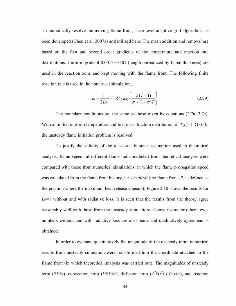
To numerically resolve the moving flame front, a ten-level adaptive grid algorithm has
been developed (Chen et al. 2007a) and utilized here. The mesh addition and removal are
based on the first and second order gradients of the temperature and reaction rate
distributions. Uniform grids of 0.00125~0.01 (length normalized by flame thickness) are
used in the reaction zone and kept moving with the flame front. The following finite
reaction rate is used in the numerical simulation,
⎥⎦
⎤⎢⎣
⎡−+−
⋅⋅⋅=T
TZZYLe )1(
)1(exp2
1 2
σσω (2.29)
The boundary conditions are the same as those given by equations (2.7a, 2.7c).
With an initial uniform temperature and fuel mass fraction distribution of T(r)=1-Y(r)=0,
the unsteady flame initiation problem is resolved.
To justify the validity of the quasi-steady state assumption used in theoretical
analysis, flame speeds at different flame radii predicted from theoretical analysis were
compared with those from numerical simulations, in which the flame propagation speed
was calculated from the flame front history, i.e. U=dR/dt (the flame front, R, is defined as
the position where the maximum heat release appears). Figure 2.10 shows the results for
Le=1 without and with radiative loss. It is seen that the results from the theory agree
reasonably well with those from the unsteady simulations. Comparisons for other Lewis
numbers without and with radiative loss are also made and qualitatively agreement is
obtained.
In order to evaluate quantitatively the magnitude of the unsteady term, numerical
results from unsteady simulation were transformed into the coordinate attached to the
flame front (in which theoretical analysis was carried out). The magnitudes of unsteady
term (∂T/∂t), convection term (U∂T/∂r), diffusion term (r-2∂(r2∂T/∂r)/∂r), and reaction
44

term (ω) in equations (2.3a, 2.3b) are evaluated and compared in the transformed
coordinate. The importance of the unsteady effects is shown by comparing the unsteady
term with other terms. Figure 2.11 shows the distributions of the unsteady, convection,
diffusion, and reaction terms in energy equation (2.3a) for flames at different flame radii
with Le=1.0 and Q=0.2. When the flame radius is large, R=5.0 in figure 2.11(a), the
unsteady term is one order smaller than all other terms, therefore it is negligible. For the
cases of larger flame radii, the unsteady term becomes much smaller. Therefore, it is
reasonable to employ the quasi-steady state assumption. When the flame radius is small,
R=0.5 in figure 2.11(b), the diffusion and reaction terms will dominate, while the
unsteady and convection terms are relatively small near the flame front. However, near
the center where energy deposition exists, the unsteady term is very large and is balanced
by the convection term. This is because the energy deposited in the center (modelled as a
boundary condition) is moving away from the flame front in the coordinate attached to
the flame front.
Furthermore, to investigate the effect of the time scale of energy deposition on the
flame trajectory, we compared the flame-front trajectories obtained from time dependent
numerical computations with different duration time, ts at a given energy flux, Q (there is
zero heat flux from the center when t>ts,). In numerical simulation, the energy flux Q at
the boundary is set to be zero when the time is greater than the duration time (ts). Figure
2.12 shows the results for Le=1.0, h=0.01 and Q=0.2. It is seen that the flame initiation
fails when the duration is too small. However, when ts≥6.5 the flame-front trajectory
(which is the same as that of ts=6.5) is not affected by the change of the time scale of
energy deposition. Therefore, in this case, the duration must be large than 6.5 (time
45

normalized by flame thickness divided by planar flame speed) to make the quasi-steady
model consistent. Similar results were also presented in (He 2000).
2.6 Conclusions
A general solution to describe the flame regimes and transitions among the flame
kernel, the flame ball, the self-extinguishing flame, the outwardly propagating spherical
flame, and the propagating planar flame is obtained. The results show that radiative heat
loss significantly affects the flame regime, flame transition, and critical ignition radius
and power. It is found that radiative loss from the unburned and burned zones play
different roles in affecting the flame propagation speed. With the increase of flame
radius, the radiative loss from the burned zone increases, while the radiative loss from the
unburned zone decreases. As a result, there is a peak radiation loss at an intermediate
flame radius, which dramatically affects the flame regimes and critical flame initiation
parameters. It is also found that the radiative loss from the unburned zone results in a new
flame regime: the isolated self-extinguishing flame with two radiation extinction limits
respectively at small and large flame radius. In addition, it is shown that the critical
Lewis number for the stationary flame ball is dominated by the heat loss from the
unburned gas. The results also show that radiative loss significantly affects the transition
history of flame initiation with external energy deposition. The critical radius for
successful flame initiation of radiative flames is much larger than that of adiabatic
flames. Furthermore, this difference increases dramatically with the increase of the Lewis
number.
46

Appendix: Solutions for Cylindrical Flames
Following the same asymptotic analysis procedure, solutions for cylindrical flame
initiation and propagation can also be obtained. The following equations provide the
general solutions for both cylindrical and spherical flames, with a geometrical factor N
utilized for these two flames (N=1, cylindrical flames; N=2, spherical flames):
⎥⎥⎦
⎤
⎢⎢⎣
⎡
−+
−==⋅Ω+⋅Ω ∫
∞−−−−
f
f
R
ULeNULeRNQf T
TZdeeRLe
QT)1(
12
exp/1σσ
ττ τ
where
⎪⎪⎪⎪⎪⎪⎪⎪⎪⎪⎪⎪⎪
⎩
⎪⎪⎪⎪⎪⎪⎪⎪⎪⎪⎪⎪⎪
⎨
⎧
≠
⎥⎦
⎤⎢⎣
⎡−−−−+−
⎥⎦
⎤⎢⎣
⎡−−−+−
+
⎥⎦
⎤⎢⎣
⎡−−−−+
⎥⎦
⎤⎢⎣
⎡−−−+
+−
≠=
⎥⎦
⎤⎢⎣
⎡−−−−+−
⎥⎦
⎤⎢⎣
⎡−−−+−
++
=≠+
⎥⎦
⎤⎢⎣
⎡−−−−+
⎥⎦
⎤⎢⎣
⎡−−−+
++
−
==
=Ω
∫
∫
∞−−
−−
∞−−−−
0
1)1(2
,1)1(2
,
1)1(2
),1(2
,
1)1(2
,1)1(2
,
1)1(2
),1(2
,
2
0,01)1(
2,1)1(
2,
1)1(2
),1(2
,
2
0,01)1(
2,1)1(
2,
1)1(2
),1(2
,
2
0,0/
21
222
222
2
111
111
112
21
222
222
22
21
111
111
11
21
hhif
kUN
kUNRkG
kUN
kUNRkG
k
kUN
kUNRkF
kUN
kUNRkF
kkk
hhif
kUN
kUNRkG
kUN
kUNRkG
kTkUT
hhifde
eR
kUN
kUNRkF
kUN
kUNRkF
kkU
hhifdeeR
ff
R
UN
URN
R
UNURN
ττ
ττ
τ
τ
⎪⎪⎪
⎩
⎪⎪⎪
⎨
⎧
≠
⎥⎥⎥⎥
⎦
⎤
⎢⎢⎢⎢
⎣
⎡
−−−+⋅+
−−−+−⋅−
=−
=Ω +−
−−
0]1)1(
2),1(
2,[
]1)1(2
),1(2
,[
0
1
1112
1111
)(5.01
1
1 hif
kUN
kUNRkFC
kUN
kUNRkGC
ek
hifeR
RkU
URN
Q
47

1
1111
111
1
1
]1)1(2
),1(2
,[
]1)1(2
,1)1(2
,[2
−
⎥⎥⎥⎥
⎦
⎤
⎢⎢⎢⎢
⎣
⎡
−−−+−+
−−−−+−+
=
kUN
kUNkGk
kUN
kUNkG
kU
CN
N
εε
εε
]1)1(2
,1)1(2
,[
]1)1(2
,1)1(2
,[
111
111
12
−−−−+
−−−−+−⋅−=
kUN
kUNRkF
kUN
kUNRkG
CC .
The effects of radiation, ignition, and Lewis number on cylindrical flame
initiation and propagation can be investigated based on the above analytical solutions in
the same way as that for spherical flames.
48
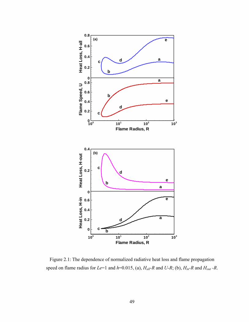
Hea
tLos
s,H
-all
0
0.2
0.4
0.6
0.8e(a)
a
b
c d
Flame Radius, R
Flam
eS
peed
,U
100 101 102 1030
0.2
0.4
0.6
0.8
e
a
b
cd
Hea
tLos
s,H
-out
0
0.2
0.4
e
(b)
ab
cd
Flame Radius, R
Hea
tLos
s,H
-in
100 101 102 103
0
0.2
0.4
0.6 e
a
bc
d
Figure 2.1: The dependence of normalized radiative heat loss and flame propagation
speed on flame radius for Le=1 and h=0.015, (a), Hall-R and U-R; (b), Hin-R and Hout -R.
49

Flame Radius, R
Flam
eS
peed
,U
10 20 300.2
0.3
0.4
0.5 a
b
cd
Hea
tLos
s,H
-all
0.1
0.2
0.3(a)
a
b
cd
Hea
tLos
s,H
-out
0.05
0.1
0.15(b)
ab
cd
Flame Radius, R
Hea
tLos
s,H
-in
10 20 300
0.1
0.2 a
bc
d
Figure 2.2: The dependence of normalized radiative heat loss and flame propagation
speed on flame radius for Le=1 and h=0.0197, (a), Hall-R and U-R; (b), Hin-R and Hout -R.
50

Flame Radius, R
Flam
eP
ropa
gatin
gS
peed
,U
10-1 100 101 102 1030
0.2
0.4
0.6
0.8
1h=0.000h=0.005h=0.015h=0.0197h=0.020
(a)
Flame Radius, R
Flam
eP
ropa
gatin
gS
peed
,U
10-1 100 101 102 1030
0.2
0.4
0.6
0.8
1h=0.000h=0.005h=0.015h=0.0197h=0.020
(b)
Figure 2.3: Flame propagation speed as a function of flame radius for Le=1.0 with
different values of radiative heat loss constants, (a), with heat losses in both the burned
and unburned zones; (b), with heat loss only in the burned zone.
51

Flame Radius, R
Flam
eP
ropa
gatin
gS
peed
,U
10-1 100 101 102 1030
0.2
0.4
0.6
0.8
1 h=0.000h=0.010h=0.025h=0.050
(a)
Flame Radius, R
Flam
eP
ropa
gatin
gS
peed
,U
10-1 100 101 102 1030
0.2
0.4
0.6
0.8
1 h=0.000h=0.010h=0.025h=0.050
(b)
Figure 2.4: Flame propagation speed as a function of flame radius for Le=0.8 with
different values of radiative heat loss constants, (a), with heat losses in both the burned
and unburned zones; (b), with heat loss only in the burned zone.
52

Flame Radius, R
Flam
eP
ropa
gatin
gS
peed
,U
100 101 102 1030
0.2
0.4
0.6
0.8
1 h=0.000h=0.010h=0.018h=0.019h=0.0195
(a)
Flame Radius, R
Flam
eP
ropa
gatin
gS
peed
,U
100 101 102 1030
0.2
0.4
0.6
0.8
1h=0.000h=0.010h=0.018h=0.019h=0.0195
(b)
Figure 2.5: Flame propagation speed as a function of flame radius for Le=1.2 with
different values of radiative heat loss constants, (a), with heat losses in both the burned
and unburned zones; (b), with heat loss only in the burned zone.
53
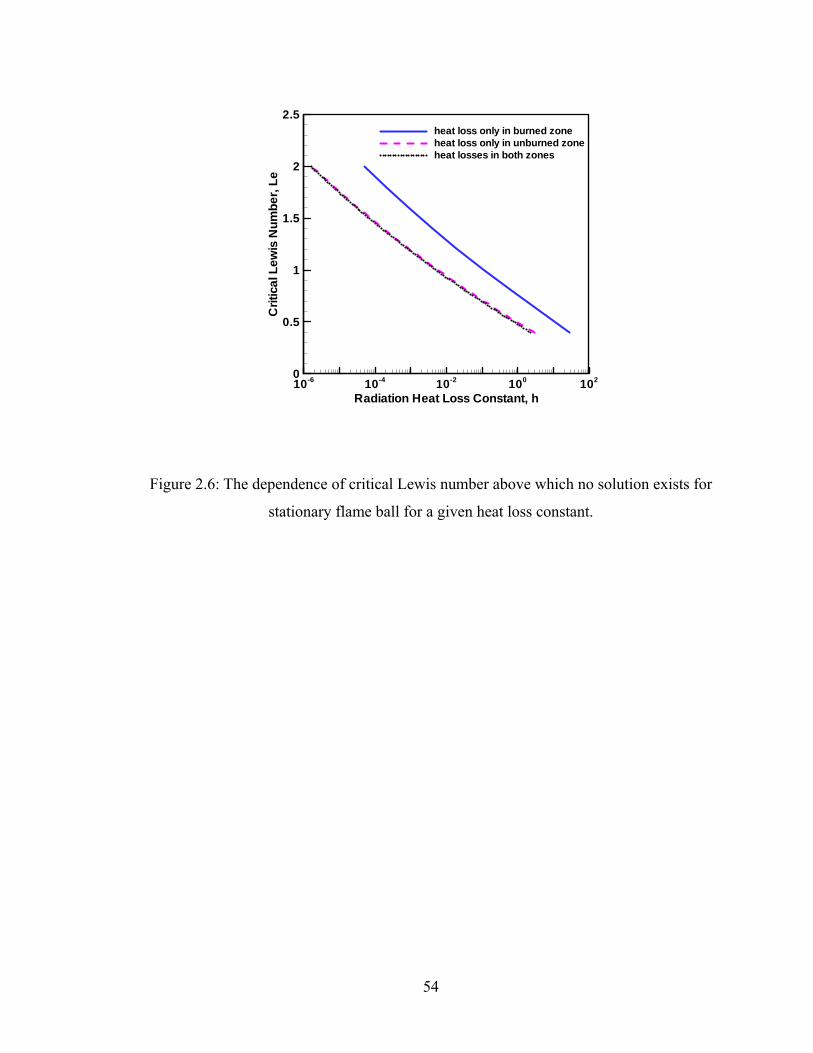
Radiation Heat Loss Constant, h
Crit
ical
Lew
isN
umbe
r,Le
10-6 10-4 10-2 100 1020
0.5
1
1.5
2
2.5heat loss only in burned zoneheat loss only in unburned zoneheat losses in both zones
Figure 2.6: The dependence of critical Lewis number above which no solution exists for
stationary flame ball for a given heat loss constant.
54
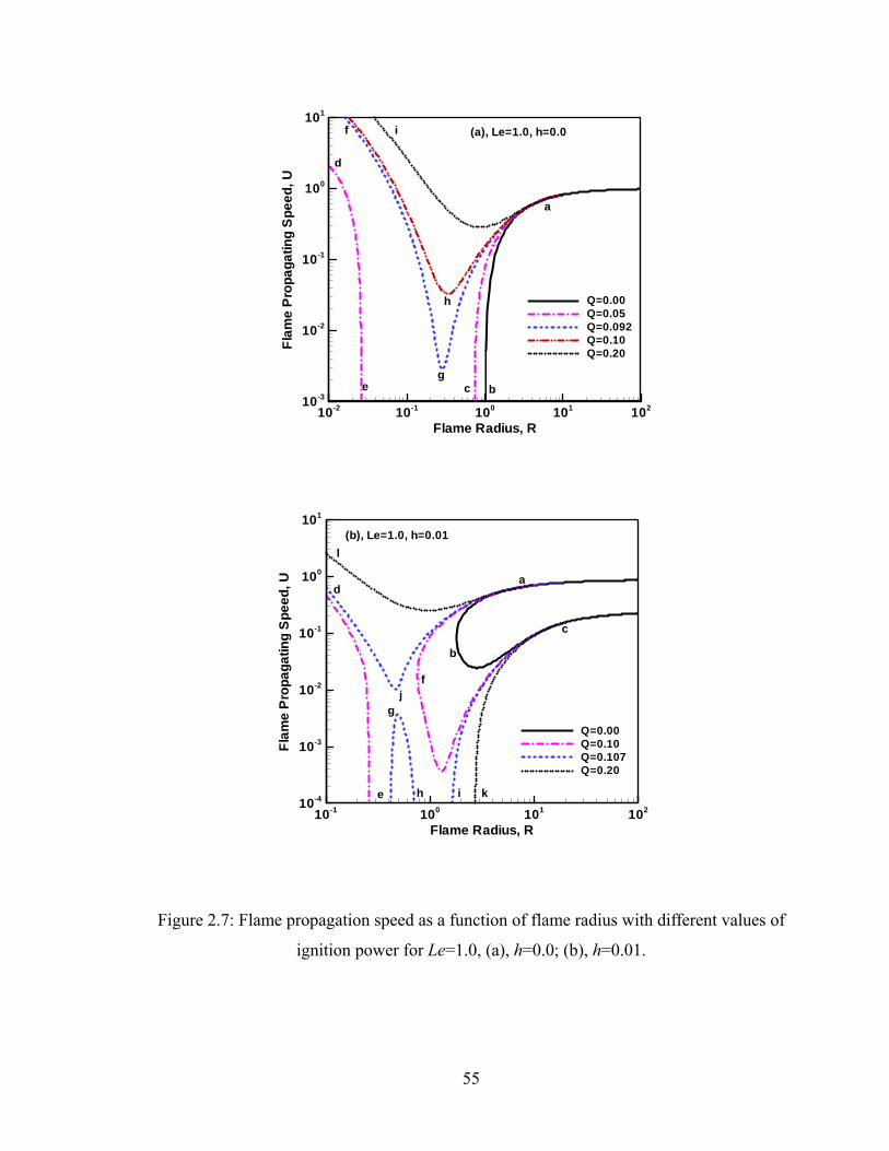
Flame Radius, R
Flam
eP
ropa
gatin
gS
peed
,U
10-2 10-1 100 101 10210-3
10-2
10-1
100
101
Q=0.00Q=0.05Q=0.092Q=0.10Q=0.20
a
bc
d
e
f
g
h
i (a), Le=1.0, h=0.0
Flame Radius, R
Flam
eP
ropa
gatin
gS
peed
,U
10-1 100 101 10210-4
10-3
10-2
10-1
100
101
Q=0.00Q=0.10Q=0.107Q=0.20
d
e
a
b
c
f
g
h i
j
l(b), Le=1.0, h=0.01
k
Figure 2.7: Flame propagation speed as a function of flame radius with different values of
ignition power for Le=1.0, (a), h=0.0; (b), h=0.01.
55

Flame Radius, R
Flam
eP
ropa
gatin
gS
peed
,U
10-2 10-1 100 101 10210-3
10-2
10-1
100
101
Q=0.000Q=0.060Q=0.064Q=0.100
(a), Le=0.8, h=0.0
ab
cdf
e
g
h
Flame Radius, R
Flam
eP
ropa
gatin
gS
peed
,U
10-2 10-1 100 101 10210-3
10-2
10-1
100
101
Q=0.000Q=0.064Q=0.068Q=0.100
(b), Le=0.8, h=0.01
ab
c d
e
eg
f
h
i
Figure 2.8: Flame propagation speed as a function of flame radius with different values of
ignition power for Le=0.8, (a), h=0.0; (b), h=0.01.
56

Flame Radius, R
Flam
eP
ropa
gatin
gS
peed
,U
10-1 100 101 10210-2
10-1
100
101
Q=0.0Q=0.1Q=0.15Q=0.6
(a), Le=1.2, h=0.0
a
b
cd
e
f
g
h
i
j
Flame Radius, R
Flam
eP
ropa
gatin
gS
peed
,U
10-1 100 101 10210-2
10-1
100
101
Q=0.0Q=0.2Q=0.5Q=0.6
(b), Le=1.2, h=0.01
a
bc
d
e
f
g
h
i
j
Figure 2.9: Flame propagation speed as a function of flame radius with different values of
ignition power for Le=1.2, (a), h=0.0; (b), h=0.01.
57

Flame Radius, R
Flam
eP
ropa
gatin
gS
peed
,U
10-2 10-1 100 101 10210-2
10-1
100
101
Q=0.07
Q=0.1
Q=0.2
(a), Le=1.0, h=0.0
Solid lines:Quasi-steady (theory)Dashed lines:Unsteady (simulation)
Flame Radius, R
Flam
eP
ropa
gatin
gS
peed
,U
10-1 100 101 10210-3
10-2
10-1
100
101
Q=0.07
Q=0.107
Q=0.2
(b), Le=1.0, h=0.01
Solid lines:Quasi-steady (theory)Dashed lines:Unsteady (simulation)
Figure 2.10: Comparison of flame propagation speeds predicted by numerical simulation
and theoretical analysis for Le=1.0, (a), h=0.0; (b), h=0.01.
58
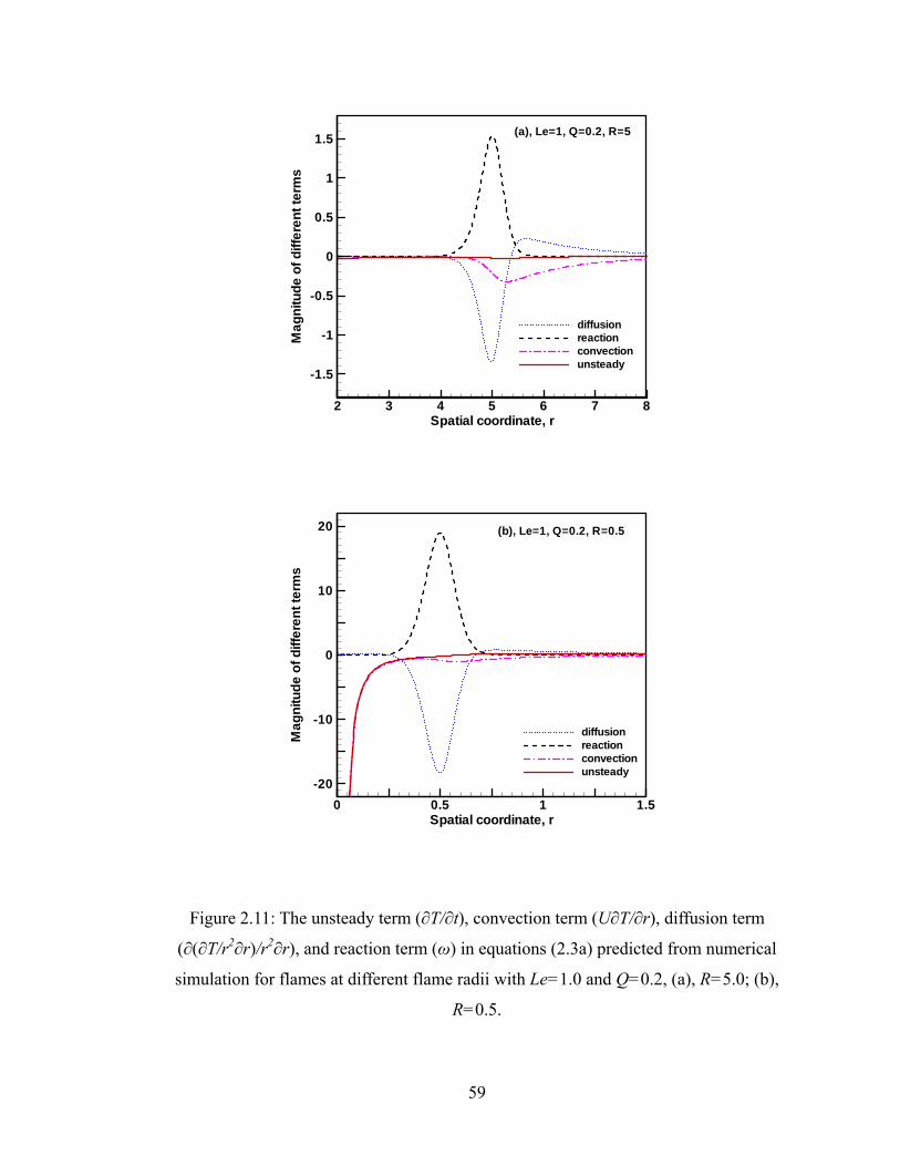
Spatial coordinate, r
Mag
nitu
deof
diffe
rent
term
s
2 3 4 5 6 7 8
-1.5
-1
-0.5
0
0.5
1
1.5
diffusionreactionconvectionunsteady
(a), Le=1, Q=0.2, R=5
Spatial coordinate, r
Mag
nitu
deof
diffe
rent
term
s
0 0.5 1-20
-10
0
10
20
diffusionreactionconvectionunsteady
1.5
(b), Le=1, Q=0.2, R=0.5
Figure 2.11: The unsteady term (∂T/∂t), convection term (U∂T/∂r), diffusion term
(∂(∂T/r2∂r)/r2∂r), and reaction term (ω) in equations (2.3a) predicted from numerical
simulation for flames at different flame radii with Le=1.0 and Q=0.2, (a), R=5.0; (b),
R=0.5.
59

Figure 2.12: Flame-front trajectories obtained from numerical computations with
different duration time (ts) at a given energy flux (Q=0.2) for Le=1.0 and h=0.01.
60

Chapter 3: Adaptive Simulation of Unsteady Reactive
Flow (A-SURF)
A time-accurate and space-adaptive numerical solver for Adaptive Simulation of
Unsteady Reactive Flow, A-SURF, has been developed. The details on the governing
equations, numerical methods, and code validations are presented in this chapter. By
using A-SURF, high-fidelity numerical simulations will be carried out to validate the
theoretical results and the kinetic models on spherical flame initiation and propagation in
the following chapters.
3.1 Governing Equations for Unsteady Reactive Flows
In A-SURF, the unsteady compressible Navier-Stokes equations are solved in
order to account for the pressure change and pressure-induced compression waves
produced during the flame propagation. The general conservation equations are presented
in Section 3.1.1. The conservation equations require modelling of the viscous stress
tensor, the diffusion velocities, the heat flux, and the chemical source terms. These
models are shown in Section 3.1.2. The detailed description and/or derivation of the
conservation and transport equations presented in this section can be found in (Williams
1985; Poinsot and Veynante 2005; Law 2006).
3.1.1 General Conservation Equations
3.1.1.1 Mass Conservation
Conservation of mass is given by the continuity equation
61

0)( =⋅∇+∂∂ V
tρρ (3.1)
where ρ is the density and V=(u, v, w) is the velocity vector.
3.1.1.2 Momentum Conservation
Conservation of momentum is described by the Navier-Stokes equations
Π⋅∇+=⋅∇+∂
∂ ∑ )()()(kk fYVV
tV ρρρ (3.2)
with fk being the body force on species k (not considered in the present study) and Π the
stress tensor, which is define as
τ+−=Π PI (3.3)
where P is the hydrostatic pressure, I the unit tensor, and τ the viscous stress tensor. In
this chapter, ∑ denotes the summation with respect to k from 1 to NS, the total number of
species.
3.1.1.3 Species Conservation
Conservation of species k is given by the species-mass-balance equation:
kkkk YVV
tY
ωρρ
=′+⋅∇+∂
∂])([
)( (3.4)
where Yk, V’k, and ωk are the mass fraction, diffusion velocity vector and the production
rate of species k, respectively. Note that the summation of the conservation equations for
each species should recover to the mass conservation equation, equation (3.1). Therefore
∑ =′ 0)( kkVYρ , ∑ = 0kω (3.5)
3.1.1.4 Energy Conservation
Conservation of total energy is described by the following equation
∑ ′+⋅++Π⋅⋅∇+⋅−∇=+⋅∇+∂∂ )]([)()]([ kkR VVfYQVqPEV
tE ρ (3.6)
62

where E, q, and QR are the total energy per unit volume, heat flux, and the heat source
term (due, for example, to an electric spark, a laser or a radiative flux), respectively. The
total energy is defined as
hVPE ρρ ++−= 2/2 , ∑= )( kk hYh , (∫+=T
T kPkk dTTChh0
)(,0, 3.7)
where T is the temperature, hk, the enthalpy of species k, hk,0 the species enthalpy of
formation at the reference temperature T0, and CP,k the specific heat of species k at
constant pressure.
3.1.1.5 Equation of State
Assuming all species in the reactive flow to be ideal gas, the equation of state that
couples density, ρ, partial pressure, Pk, and temperature, T, reads
kkk MTRYP /0ρ= (3.8)
where R0 is the universal gas constant (8.314 J/(molK)) and Mk is the molecular weight of
species k. The hydrostatic pressure P is equal to the summation of the partial pressures Pk
of all species
MTRPP k /0ρ== ∑ (3.9)
with ])/(/[1 ∑= kk MYM being the mean molecular weight of the mixture.
3.1.2 Transport and Chemistry Models
3.1.2.1 Viscous Stress
The gas mixture is assumed to behave as a Newtonian fluid. Therefore, the
viscous stress tensor can be modelled with Stokes’ law of friction,
])(32)([( IVVVPI T ⋅∇−∇+∇+−=Π μ (3.10)
63

where μ is the dynamic viscosity of the mixture. Note that Stokes’ assumption of zero
bulk viscosity is employed here.
3.1.2.2 Diffusion Velocity
The diffusion velocity can be obtained by solving the following system of
equations
NSiTT
YD
YD
DXX
ffYYPP
PXYVVD
XXX
i
iT
j
jTNS
j ji
ji
ji
NS
jjiiiij
NS
j ji
jii
,...,1))(()(
)()())(()()(
,,
1 ,
11 ,
=∇
−+
−+∇
−+′−′=∇
∑
∑∑
=
==
ρ
ρ
(3.11)
where Di,j is the binary mass diffusion coefficient of species i into species j,
kkk MMYX /= the mole fraction, and DT,k the thermal diffusion (the diffusion of mass
due to temperature gradients: Soret effect) coefficient of species k. Mathematically, it is
difficult and costly to solve these equations and simplified approach (for example Fick’s
law) is usually used. In the present study, the mixture-averaged formula (Kee et al. 1985)
is employed. The diffusion velocity is composed of three parts (Kee et al. 1985):
CkTkYkk VVVV ,,, ′+′+′=′ (3.12)
where V’k,Y is the ordinary diffusion velocity and is given in the Curtiss-Hirschfelder
approximation by
MMYDVY kkmYkk /)(, ∇−=′ (3.13)
and Dkm is the mixture-averaged diffusion coefficient of species k.
Furthermore, V’k,T is the thermal diffusion velocity, which is included only for
low molecular weight species (H, H2 and He)
)/(, MTTMDVY kkkmTkk ∇Θ−=′ (3.14)
64
where Θk is the thermal diffusion ratio of species k, the sign of which makes the lower
molecular weight species diffuse from low to high temperature regions.
The correction velocity V’k,C is included to insure compatibility of species and
mass conservation equations. It is calculated according to the requirement given by the
first equation in (3.5).
3.1.2.3 Heat Flux
The heat flux q includes a heat diffusion term expressed by the Fourier’s law and
a second term associated with the diffusion of species with different enthalpies.
∑ ′+∇−= kkk VYhTq ρλ (3.15)
where λ is the thermal conductivity of the gas mixture. Note that the Dufour effect (heat
flux due to a mass gradient) is usually negligible and thus is not included in the present
study.
In A-SURF, the CHEMKIN-TRANSPROT package (Kee et al. 1989) is
implemented to calculate all the transport coefficients, μ, Dkm, Θk, and λ.
3.1.2.4 Chemical Model
Consider a chemical system of NS species reacting through NR reactions
NRjforAA kjkkjk ,...,1"' ,, =⇔ ∑∑ νν (3.16)
where Ak is a symbol for species k, ν’k,j and ν”k,j are the molar stoichiometric coefficients
of species k in reaction j. The production rate of species k is given by a general form of
the law of mass action
∑=
Ψ−=NR
jjjkjkkk M
1,, )'"( ννω (3.17)
where Ψj is the progress rate of reaction j, written as
65

jkjk
k
kNSkjb
k
kNSkjfj M
YKMYK ,, "
1,'
1, )()( νν ρρ== Π−Π=Ψ (3.18)
where Kf,j and Kb,j are the forward and reverse rates of reaction j. The reaction rate for
each elementary reaction is usually modeled using the empirical Arrhenius law
)exp(,, RTE
TAK jjfjf
j −= β (3.19)
where Af,j is the pre-exponential constant, βj the temperature exponent, and Ej the
activation energy. These parameters are given by the detailed reaction mechanism and the
CHEMKIN package (Kee et al. 1985; Kee et al. 1989) is used to evaluate the production
rate.
In A-SURF, different detailed chemical mechanisms are utilized for different
fuels. For example, the recent mechanism of 9 species and 25 reactions developed by Li
et al. (Li et al. 2004) is employed for H2/air flames, and the GRI-MECH 3.0 mechanism
(Smith et al.) is utilized for CH4/air flames.
3.2 Numerical Methods
Finite volume method is employed for discretizing the governing equations given
in the previous section. The conservation equations for one-dimensional,
multi-component, reactive compressible flows can be written as
)()()()( US
xUF
xUGN
xUF
tU
Rv +∂
∂=+
∂∂
+∂
∂ (3.20)
where the vectors U, F(U), G(U), Fv(U), and SR(U) are defined as
66

⎟⎟⎟⎟⎟⎟⎟⎟
⎠
⎞
⎜⎜⎜⎜⎜⎜⎜⎜
⎝
⎛
=
Eu
Y
YY
UNS
ρρ
ρρ
M2
1
, , ,
⎟⎟⎟⎟⎟⎟⎟⎟
⎠
⎞
⎜⎜⎜⎜⎜⎜⎜⎜
⎝
⎛
++
=
uPEPu
uY
uYuY
UFNS
)(
)(
2
2
1
ρρ
ρρ
M
⎟⎟⎟⎟⎟⎟⎟⎟
⎠
⎞
⎜⎜⎜⎜⎜⎜⎜⎜
⎝
⎛
+
=
uPEu
uY
uYuY
UGNS
)(
)(
2
2
1
ρρ
ρρ
M
⎟⎟⎟⎟⎟⎟⎟⎟
⎠
⎞
⎜⎜⎜⎜⎜⎜⎜⎜
⎝
⎛
+Φ+−−
′−
′−
′−
=
−
−
−
−
−
RN
xNN
xNSNSNN
xNN
xNN
v
QqxxNxx
VYxx
VYxxVYxx
UF
/)()(
)()(
)(
21
22
11
ττρ
ρρ
M, (
⎟⎟⎟⎟⎟⎟⎟⎟
⎠
⎞
⎜⎜⎜⎜⎜⎜⎜⎜
⎝
⎛
=
00
2
1
NSRS
ω
ωω
M3.21)
where N is the geometry factor (N=0, rectangular coordinate; N=1, cylindrical coordinate;
N=2 spherical coordinate). u is the flow velocity and x(=r) is the spatial coordinate.
The viscous stress and dissipation energy are:
}]/)()[3/2()/(2)/(2{'']//)([
/)()3/2(/2/)()3/2(/2
22221
2
1
xuxxxuNxuxNxxxu
xuxxxuxuxxxu
NN
NN
NN
NN
∂∂−+∂∂=Φ
Φ+−∂∂=Φ
∂∂−=
∂∂−∂∂=
−
−
−
−
μ
ττ
μμτ
μμτ
(3.22)
The heat flux is:
∑ ′+∂∂−= )(/ kkkNN VYhxxTKxq ρ (3.23)
The corrected diffusion velocities (to ensure 0=′∑ kkVY ) are:
∑ ∇Θ+∇=′
′−∇Θ+∇=′−
)]/(/)([
)/(/)(
,
,
MTTMDMMYDVwith
VYMTTMDMMYDVY
kkkmkkmCk
Ckkkkkmkkmkk (3.24)
3.2.1 Fractional-step Procedure
To solve the conservation system (3.20), the stiff source term SR is treated by the
67

fractional-step procedure (Toro 1999). In the first fractional step, the non-reactive flow is
solved
1
),(:
)()()(: +⇒⎪⎭
⎪⎬⎫
=∂
∂=+
∂∂
+∂
∂n
nn
v
UUtxUIC
xUF
xUGN
xUF
tUPDE (3.25)
The chemistry is solved in the second fractional step for a homogeneous system
1
1:
)(: +
+⇒
⎪⎭
⎪⎬⎫= n
n
R UUIC
USdt
dUODE (3.26)
The two steps given by equations (3.25) and (3.26) are denoted by operator C(t)
and operator S(t), respectively. Based on the above splitting, the solution can be evolved
from its initial value Un at time tn, by one time step of size Δt, to a value Un+1 at time
tn+1= tn+Δt,
)(1 nttn UCSU ΔΔ+ = (3.27)
The above procedure for solving the inhomogeneous system given by equation
(3.20) is exceedingly simple but only has first-order accuracy in time, when S and C are
at least first-order accurate solution operators (Toro 1999). A scheme with second-order
accuracy in time called Strang splitting (Strang 1968) is
)(2/2/1 ntttn USCSU ΔΔΔ+ = (3.28)
where S and C are at least second-order accurate solution operators in time.
For the S operator, the mass fraction of species are updated by using the VODE
solver (Brown et al. 1989). Note that the density ρ, momentum ρu, and total energy E
remain to be constant during updating the mass fraction of all the species, after which the
temperature is solved according to the definition of total energy, equation (3.7):
0/2//)( 20 =+−−= ρEhuMTRTF (3.29)
68
where the equation of state, equation (3.9), is utilized to eliminate the pressure term. The
above equation can be solved numerically by using the Newton iteration method and the
updated temperature at each iteration step is
)//()( 0P
oldoldnew CMRTFTT −−= (3.30)
For the C operator, the details are presented in the following.
3.2.2 Finite Volume Method
The unsteady convection-diffusion system solved in the C operator is discretized
by applying a Godunov-type upwind finite volume spatial discretization procedure (Toro
1999). The integral form of the conservation system (3.20) without the source term is
∫∫∫∫ ∂∂
=+∂
∂+
∂∂ dx
xUFdx
xUNGdx
xUFdx
tU v )()()( (3.31)
A conservative finite-volume scheme can be obtained by evaluating the integral
over a control volume representing the domain of interest. Here we consider the control
volume over space from xi-1/2 to xi+1/2. For this control volume, the above equation
becomes
)],(),([
)()],(),([),(
2/12/1
2/12/12/1
2/1
2/1
2/1
txFtxF
dxxUNGtxFtxFdxtxU
dtd
iviv
x
xii
x
x
i
i
i
i
−+
−+
−=
+−+ ∫∫+
−
+
− (3.32)
Explicit time marching (Toro 1999) is utilized in the C operator and the above
equation is solved to evolve the solution from the current time step tn to the next time step
tn+1= tn+Δt, where Δt is the time step length which is restricted by the CFL number for
computational stability (Toro 1999).
The MUSCL-Hancock (van Leer 1984) and central difference schemes, both of
second-order accuracy, are employed to evaluate the convective flux, F(xi+1/2,t), and
69

diffusive flux, Fv(xi+1/2,t), in equation (3.32), respectively. The ordinary differential
equation, (3.32), can be written in the following form
)(ULdtUd
= (3.33)
where U is the cell average of the solution state. At cell i, it is
∫+
−−+ −=
2/1
2/1
),(1)(2/12/1
i
i
x
xii
i dxtxUxx
tU (3.34)
To update the state nU at the current time step to state 1+nU at the next time
step according to equation (3.33), a second-order TVD Runge-Kutta method (Gottlieb
and Shu 1998) can be utilized
)(21
21
21
)(
)1()1(1
)1(
UtLUUU
UtLUU
nn
nn
Δ++=
Δ+=
+ (3.35)
3.2.3 Locally Adaptive Mesh
Most combustion phenomena in nature contain many disparate length scales.
Therefore, a numerical method should be able to adapt resolutions to regions with
different length scales; otherwise computer resources will be largely wasted in regions
where the solutions do not require the maximum resolution. Mesh adaptation is just a
way to distribute mesh cells in the interested regions so as to resolve a physical
phenomenon economically.
An unstructured h-refinement (the cells in the regions of interest are locally
subdivided, and some other cells may be coarsened in the regions of less importance) is
employed in A-SURF. Local mesh addition and removal are based on the first-order and
second-order gradients of the temperature, velocity and major species distributions. The
70

present adaptive mesh for one-dimensional and two-dimensional simulations is based on
the same algorithm developed in (Sun 1998; Sun and Takayama 1999). The details can be
found in (Sun 1998; Sun and Takayama 1999) and thus not repeated here.
For propagating flames investigated in the present study, the reaction zone is
usually very thin and the flame thickness is strongly affected by pressure. Therefore, in
order to maintain adequate numerical resolution of a moving flame front without the need
to use hundreds of thousands of grid points, adaptive mesh with seven to ten grid levels is
utilized in this study and the moving reaction zone is always fully covered by the finest
meshes of 32 μm to 4 μm in width.
It is noted that the numerical methods described above are for one-dimensional
reactive flows whose conservation equations are given in (3.20). For two-dimensional
problems, the same fractional-step procedure and finite volume method are implemented
in A-SURF.
3.3 Validation and Examples
To demonstrate the accuracy and robustness of A-SURF, simulation results from
A-SURF for different problems are compared with their exact solutions or predictions by
other well-developed algorithms.
Simulation of a modified version of the popular Sod’s test (Sod 1978; Toro 1999)
is carried out to illustrate the performance of A-SURF on one-dimensional, time
dependent Euler equations. Figure 3.1 shows the comparison between numerical and
exact solutions of the temperature distribution. It is seen that the left-propagating
expansion fan, right-propagating contact line, and right-propagating shock wave are all
well resolved and the numerical prediction agrees well with the exact solution. Moreover,
71

according to the mesh level distribution (the mesh size is inversely proportional to 2mesh
level), the finest meshes are focused on the expansion fan, contact line, and shock wave.
Therefore, the adaptive mesh utilized in A-SURF helps to resolve these physical
phenomena economically.
A one-dimensional, time dependent convection-diffusion problem is utilized to
show the performance of A-SURF on the Navier-Stokes equations. The governing
equations and initial conditions for unsteady convection (with constant velocity, u) and
diffusion (at constant mass diffusivity, DH2) of hydrogen can be written as (assuming
constant density, ρ(x,t)≡1)
)()(222
2
2
2
HHHH YD
dxduY
dxd
dtdY
=+ (3.36)
⎩⎨⎧
><
==cmxcmx
txYH 200.02006.0
)0,(2
(3.37)
The above problem has the following exact solution
)2
(03.003.0),(2
2 tDutxerftxY
HH ⋅
−⋅−= , with ∫ −=
y S dseyerf0
22)(π
(3.38)
Figure 3.2 shows the hydrogen mass fraction profiles at different times. The numerical
prediction by A-SURF is seen to agree very well with the exact solution given by
equation (3.38). Also it is seen that the finest meshes are focused on the region with large
gradient of hydrogen mass fraction due to the mesh adaptation. Therefore, A-SURF could
be utilized to accurately and efficiently simulate one-dimensional unsteady
convection-diffusion problems.
To illustrate the performance of A-SURF on one-dimensional propagating flames,
PREMIX (Kee et al. 1985) is employed here to make comparison with A-SURF since
72
PREMIX is widely utilized to simulate one-dimensional planar flames in combustion
research. Figure 3.3 shows the simulation results for a planar stoichiometric CH4/air
flame from both A-SURF and PREMIX. The GRI-MECH 3.0 mechanism (Smith et al.) is
utilized in both simulations. It is seen that the temperature distribution predicted by
A-SURF is nearly the same as that by PREMIX. The relative differences of adiabatic
flame temperature, Tad, and laminar flame speed, Su, between the predictions by A-SURF
and PREMIX are 0.27% and 1.34%, respectively. Simulations of one-dimensional planar
flames for other fuels were also conducted and very good agreements between
predictions from A-SURF and PREMIX were obtained. Therefore, A-SURF can
accurately model one-dimensional flames.
Figure 3.4 shows the temperature and mesh level distribution at different times for
a propagating spherical CH4/O2/CO2 (15%/30%/55% by volume) flame (the
spectral-dependent radiation, discussed in Chapter 6, is not considered here). The flame
front is shown to be covered by the finest meshes (L=6 in mesh level and ∆x=16 μm in
mesh size). Moreover, the finest meshes move together with the flame front and thus the
total mesh number does change during flame propagation. Figure 3.5 shows the flame
propagation speed as a function of flame radius for different propagating spherical H2/air
and CH4/air flames. The computation domain is a sphere of 30 cm in radius, which is the
same that of the spherical chamber used in experiments (Taylor 1991). As shown in
figure 3.5, good agreement between simulations and experiments is obtained. The
laminar flame speeds of methane/air at different equivalence ratios from simulations
(predicted by both A-SURF and PREMIX) and experiments (Gu et al. 2000; Rozenchan
et al. 2003; Qin and Ju 2005) are shown in figure 3.6. It is observed that the laminar
73

flame speeds of methane/air predicted by A-SURF agree very well with those by
PREMIX and the experimental results. The maximum relative differences between the
predictions from A-SURF and PREMIX over the entire test range is less than 2%, which
demonstrates the robustness and accuracy of the present computation methods. The
laminar flame speeds and burned Markstein length of hydrogen/air flames as a function
of equivalence ratio are shown in figure 3.7. Again, very good agreement among the
predictions from A-SURF and PREMIX is obtained. According to all the tests shown in
figures 3.3 to 3.7, A-SURF can accurately model the propagating flames. Therefore, it
can be employed to validate the theoretical models for spherical flame initiation and
propagation in the following chapters. To the authors’ knowledge, A-SURF is currently
the only code available to simulate propagating flames based on compressible governing
equations (thus acoustics are resolved) using detailed chemical mechanisms and an
adaptive mesh.
The above discussion is on one-dimensional problems. Some preliminary results
on two-dimensional simulations using A-SURF are shown in figures 3.8 to 3.12.
In order to demonstrate the performance of two-dimensional adaptive mesh
utilized in A-SURF, a propagating flame with specified propagating flame front,
Rf(t)=(Rf0+U·t)·[1+0.05·sin(24·θ)], is studied. No flow is considered in the simulation and
mesh adaptation is based on the temperature gradient which changes with the propagation
of the flame front, Rf(t). The temperature distribution is given by
⎟⎟
⎠
⎞
⎜⎜
⎝
⎛−
+=
+−
−= 1)(
2001110001300),,(
22
tRyx
SwitheetyxT
fS
S
(3.39)
Therefore, the temperature of the unburned and burned gases is 300 K and 2300 K,
74

respectively. Adaptive mesh spanned seven levels, from the base mesh, level L=0, to the
finest mesh, level L=6 (mesh size changes from 2048 × 2048 μm2 to 32 × 32 μm2 for the
rectangular meshes shown in figure 3.8) are implemented in the simulation. Figure 3.8
shows that the flame front is covered by the finest mesh (which moves together will the
flame front) due to the appearance of the largest temperature gradient there, and that both
quadrilateral and rectangular meshes can be utilized in the simulation. Therefore, this
example shows that A-SURF can efficiently resolve two-dimensional propagating flames
using locally adaptive meshes. Moreover, with the help of quadrilateral meshes, any
two-dimensional computational domain with arbitrary boundary geometries can be
accurately resolved by A-SURF.
To illustrate the performance of A-SURF on two-dimensional, time dependent
Euler equations, a numerical simulation of cylindrical explosion by A-SURF was
conducted. For this problem, the initial conditions are described by two thermodynamic
states separated by a cylindrical interface: high pressure state inside and low pressure
state outside. During the evolvement, an outwardly-propagating shock, an
outwardly-propagating contact surface, and an inwardly-propagating rarefaction wave
appear. This is similar to the Sod’s problem (Sod 1978; Toro 1999) discussed at the
beginning of this section. Due to the axisymmetry of this problem, it can be studied by
both one-dimensional and two-dimensional simulations. Figure 3.9(a) shows a
comparison between the one-dimensional radial solution (very high resolution which
could be regarded as the exact solution) and the two-dimensional solution along the radial
line that is coincident with the x-axis. It is seen that the prediction from the
two-dimensional simulation agrees very well with the exact solution. Comparison along
75
other radial directions gives virtually identical results. This is confirmed by the very
symmetric character of the numerical solution of density distribution shown in figure
3.9(b), demonstrating that A-SURF can accurately resolve the rarefaction wave, contact
surface, and shock wave in two-dimensional simulations. Similar to the one-dimensional
simulation shown in figure 3.1, the finest meshes are focused on the expansion fan,
contact line, and shock in the two-dimensional simulation. Moreover, nearly the same
results were obtained from simulations using rectangular and quadrilateral meshes
(similar to the two types of meshes shown in figure 3.8).
Another example of the two-dimensional simulation based on Euler equations is
shown in figure 3.10. The wave interaction problem (Müller 2000) is studied using
A-SURF. The initial configuration is determined by four states corresponding to the four
quadrants of the coordinate system (Müller 2000):
⎩⎨⎧
<⋅≥⋅
=0)4,/0,/0,/4(0)1,/1,/1,/1(
),,,( 3
3
yxifatmsmsmmKgyxifatmsmsmmKg
Puu yxρ (3.40)
Away from the origin of the coordinate system, the solution, as shown in figure 3.10(a),
exhibits a one-dimensional wave pattern consisting of a rarefaction wave, a contact
surface and a shock wave. Close to the origin, the different one-dimensional waves
interact forming a genuinely two-dimensional wave pattern. The density contours shown
in figure 3.10(a) agree well with those reported in (Müller 2000). Moreover, figure 3.10(b)
shows that the finest adaptive meshes efficiently cover the position where the waves and
their interactions appear. These results show that the two-dimensional simulation can
accurately resolve the wave interactions.
A-SURF is also utilized to simulate propagating two-dimensional premixed
flames with one-step irreversible chemical mechanism. Figures 3.11 and 3.12 show the
76
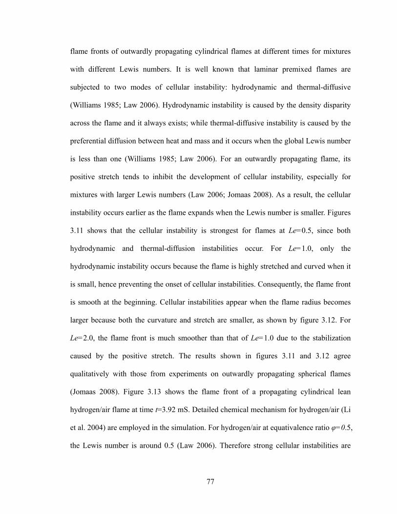
flame fronts of outwardly propagating cylindrical flames at different times for mixtures
with different Lewis numbers. It is well known that laminar premixed flames are
subjected to two modes of cellular instability: hydrodynamic and thermal-diffusive
(Williams 1985; Law 2006). Hydrodynamic instability is caused by the density disparity
across the flame and it always exists; while thermal-diffusive instability is caused by the
preferential diffusion between heat and mass and it occurs when the global Lewis number
is less than one (Williams 1985; Law 2006). For an outwardly propagating flame, its
positive stretch tends to inhibit the development of cellular instability, especially for
mixtures with larger Lewis numbers (Law 2006; Jomaas 2008). As a result, the cellular
instability occurs earlier as the flame expands when the Lewis number is smaller. Figures
3.11 shows that the cellular instability is strongest for flames at Le=0.5, since both
hydrodynamic and thermal-diffusion instabilities occur. For Le=1.0, only the
hydrodynamic instability occurs because the flame is highly stretched and curved when it
is small, hence preventing the onset of cellular instabilities. Consequently, the flame front
is smooth at the beginning. Cellular instabilities appear when the flame radius becomes
larger because both the curvature and stretch are smaller, as shown by figure 3.12. For
Le=2.0, the flame front is much smoother than that of Le=1.0 due to the stabilization
caused by the positive stretch. The results shown in figures 3.11 and 3.12 agree
qualitatively with those from experiments on outwardly propagating spherical flames
(Jomaas 2008). Figure 3.13 shows the flame front of a propagating cylindrical lean
hydrogen/air flame at time t=3.92 mS. Detailed chemical mechanism for hydrogen/air (Li
et al. 2004) are employed in the simulation. For hydrogen/air at equativalence ratio φ=0.5,
the Lewis number is around 0.5 (Law 2006). Therefore strong cellular instabilities are
77

observerd.
In summary, based on the numerical validations and tests presented above,
A-SURF can be utilized to accurately and efficiently simulate one-dimensional
propagating flames with detailed chemical mechanisms. For two-dimensional flame
simulations with large detailed chemistry (for large hydrocarbon fuels) treated by a single
computer, the computation time will be on the order of a month and thus effective
parallelization and chemical mechanism reduction are needed. In the following chapters,
only one-dimensional simulations using A-SURF will be conducted.
78

X (cm)
Tem
pera
ture
(K)
Mes
hLe
vel
0 0.05 0.1 0.15 0.2 0.25260
280
300
320
340
360
380
400
420
-6
-4
-2
0
2
4
6expansion fan contcat line shock
numericalexact
Figure 3.1: Mesh level and temperature distribution at time t=100 μs.
X (cm)
YH
2
20 25 30
0
0.01
0.02
0.03
0.04
0.05
0.06
exactnumerical
X (cm)
YH
2
31.9 31.95 32 32.05 32.1
0
0.01
0.02
0.03
0.04
0.05
0.06
exactnumerical
(a) (b)
Figure 3.2: Distribution of hydrogen mass fraction: (a) at time t=0, 19200, 38400, 57600,
76800 μs with u=1 m/s and DH2=8·10-5 m2/s; (b) at t=120 μs with u=1000 m/s and
DH2=8·10-5 m2/s.
79
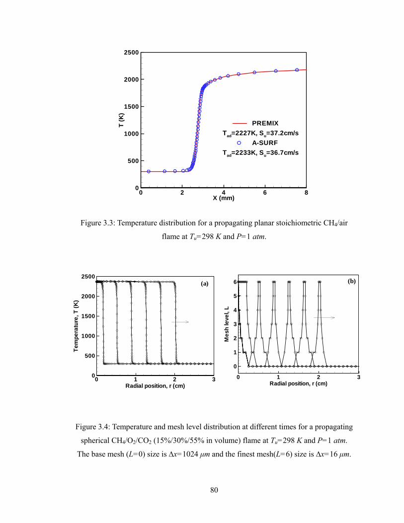
X (mm)
T(K
)
0 2 4 6 80
500
1000
1500
2000
2500
PREMIXTad=2227K, Su=37.2cm/s
A-SURFTad=2233K, Su=36.7cm/s
Figure 3.3: Temperature distribution for a propagating planar stoichiometric CH4/air
flame at Tu=298 K and P=1 atm.
Radial position, r (cm)
Tem
pera
ture
,T(K
)
0 1 2 30
500
1000
1500
2000
2500
Radial position, r (cm)
Mes
hle
vel,
L
0 1 2 3
0
1
2
3
4
5
6 (b)(a)
Figure 3.4: Temperature and mesh level distribution at different times for a propagating
spherical CH4/O2/CO2 (15%/30%/55% in volume) flame at Tu=298 K and P=1 atm.
The base mesh (L=0) size is ∆x=1024 μm and the finest mesh(L=6) size is ∆x=16 μm.
80

XXXX XX X X X X X X X X X X X X X X X X X X X X X X X Xϕ = 1.0, CH4/air
Flame radius, Rf (cm)
Flam
epr
opag
atin
gsp
eed,
Sb
(cm
/s)
0 1 2 30
400
800
1200
1600
4
= 4.5, H2/airϕ
ϕ = 3.0, H2/air
Lines: simulation (A-SURF)Symbols: experiment (Taylor, 1991)
ϕ = 1.0, H2/air
Figure 3.5: Flame propagation speed as a function of flame radius for different spherical
H2/air and CH4/air flames.
Equivalence ratio,
Lam
inar
flam
esp
eed,
Su0
(cm
/s)
0.6 0.8 1 1.2 1.4
10
20
30
40
A-SURFPREMIXGu et al. (2000)Rozenchan et al. (2002)Qin and Ju (2005)
ϕ
CH4/air, 1 atm
Figure 3.6: Laminar flame speed of CH4/air flames as a function of equivalence ratio at
Tu=298 K and P=1 atm.
81
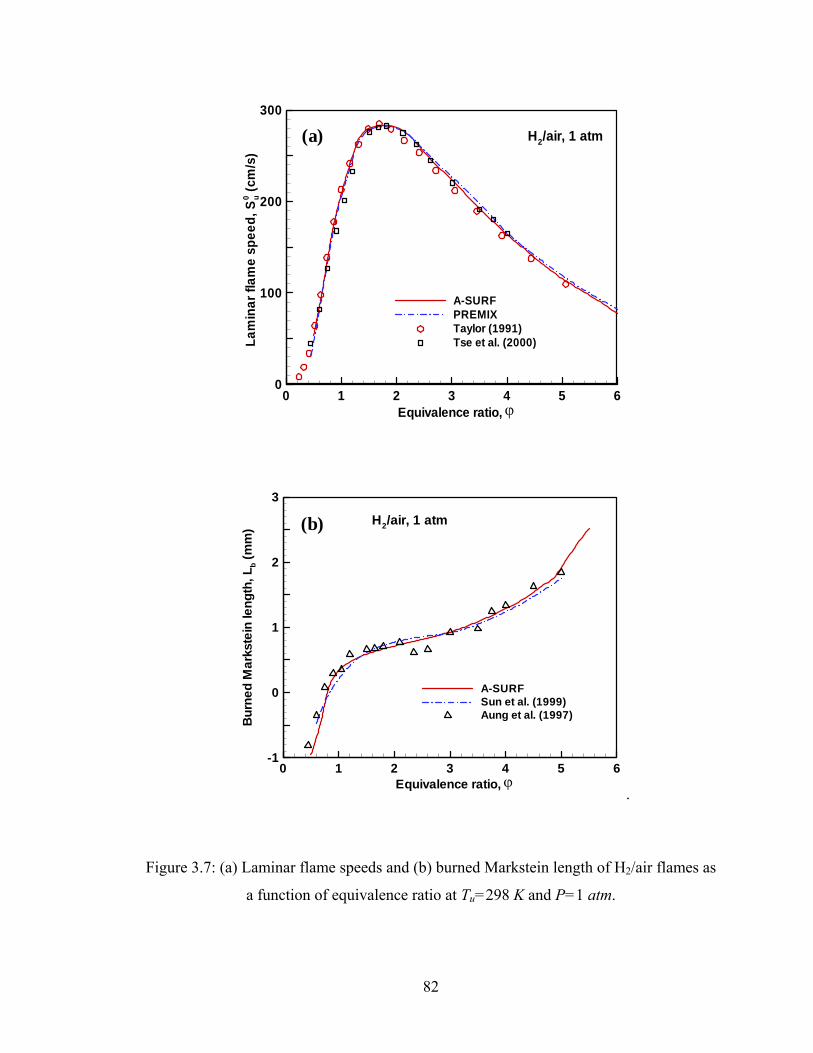
Equivalence ratio,
Lam
inar
flam
esp
eed,
Su0
(cm
/s)
0 1 2 3 4 5 60
100
200
300
A-SURFPREMIXTaylor (1991)Tse et al. (2000)
(a)
ϕ
H2/air, 1 atm
Equivalence ratio,
Bur
ned
Mar
kste
inle
ngth
,Lb
(mm
)
0 1 2 3 4 5-1
0
1
2
3
A-SURFSun et al. (1999)Aung et al. (1997)
6ϕ
H2/air, 1 atm
.
(b)
Figure 3.7: (a) Laminar flame speeds and (b) burned Markstein length of H2/air flames as
a function of equivalence ratio at Tu=298 K and P=1 atm.
82
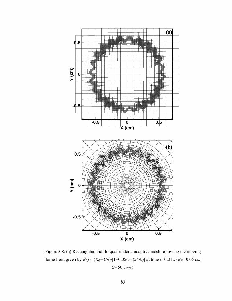
X (cm)
Y(c
m)
-0.5 0 0.5
-0.5
0
0.5
(a)
X (cm)
Y(c
m)
-0.5 0 0.5
-0.5
0
0.5
(b)
Figure 3.8: (a) Rectangular and (b) quadrilateral adaptive mesh following the moving
flame front given by Rf(t)=(Rf0+U·t)·[1+0.05·sin(24·θ)] at time t=0.01 s (Rf0=0.05 cm,
U=50 cm/s).
83

Spatial coordinate, r (cm)
Den
sity
(Kg/
m3 )
0 0.5 1 1.5 2 2.50.6
0.8
1
1.2
1.4
1.6
1.8
exact2D
(a) Cylindrical explosion
Initial T = 298KP = 2 atm for r < 1cmP = 1 atm for r > 1cm
Output at 1.6E-5 second
(b)
Figure 3.9: Two dimensional simulation of cylindrical explosion: (a), comparison
between the exact and 2D solutions; (b), the density distribution.
84

(a)
(b)
Figure 3.10: Two dimensional simulation of wave interactions: (a), density contours; (b),
adaptive mesh. Output time: 12 μs; mesh size: ∆x0=5 mm, ∆x=∆x0/2Level.
85
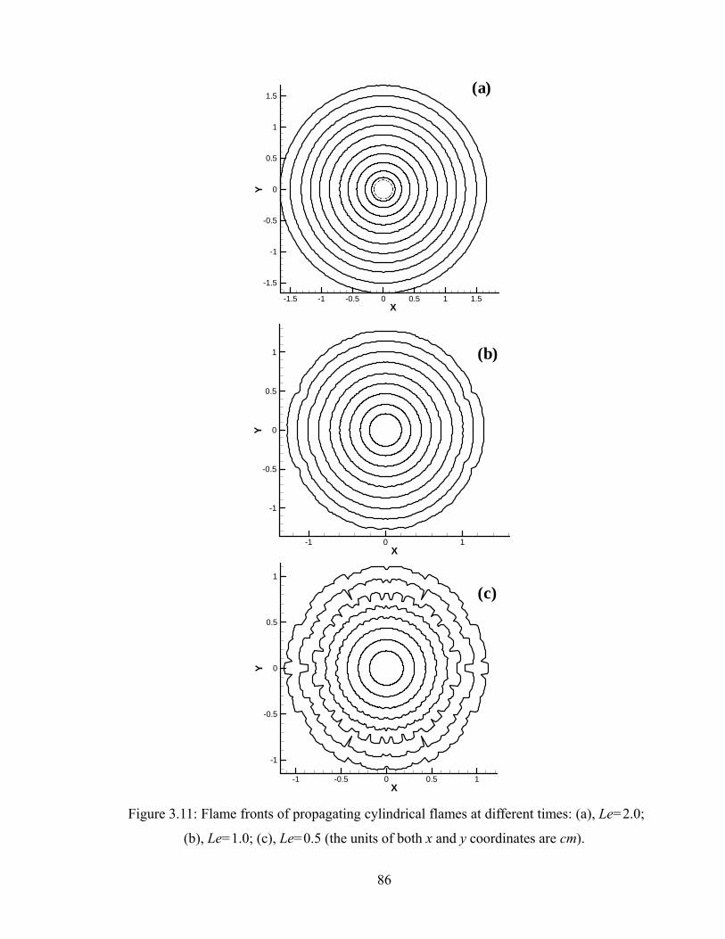
X
Y
-1.5 -1 -0.5 0 0.5 1 1.5
-1.5
-1
-0.5
0
0.5
1
1.5(a)
X
Y
-1 0 1
-1
-0.5
0
0.5
1
X
Y
-1 -0.5 0 0.5 1
-1
-0.5
0
0.5
1
(b)
(c)
Figure 3.11: Flame fronts of propagating cylindrical flames at different times: (a), Le=2.0;
(b), Le=1.0; (c), Le=0.5 (the units of both x and y coordinates are cm).
86
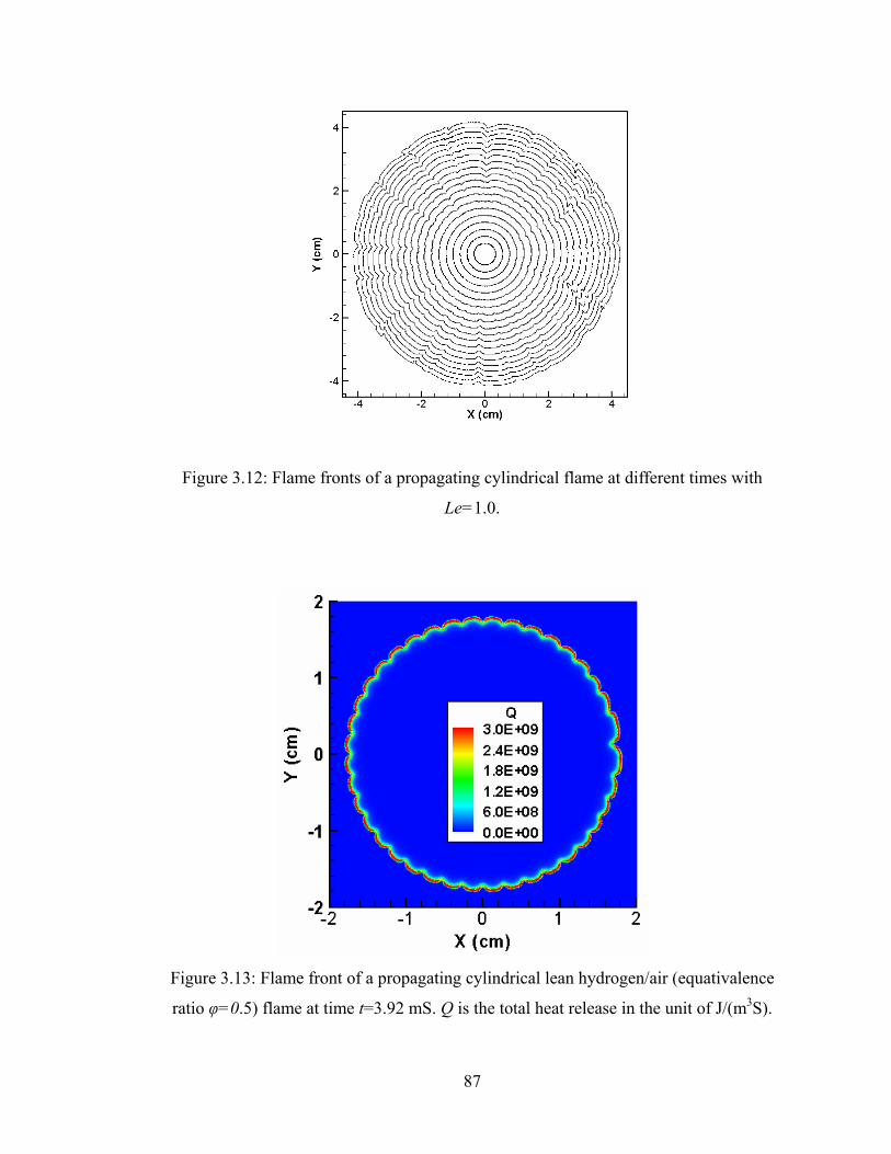
Figure 3.12: Flame fronts of a propagating cylindrical flame at different times with
Le=1.0.
Figure 3.13: Flame front of a propagating cylindrical lean hydrogen/air (equativalence
ratio φ=0.5) flame at time t=3.92 mS. Q is the total heat release in the unit of J/(m3S).
87
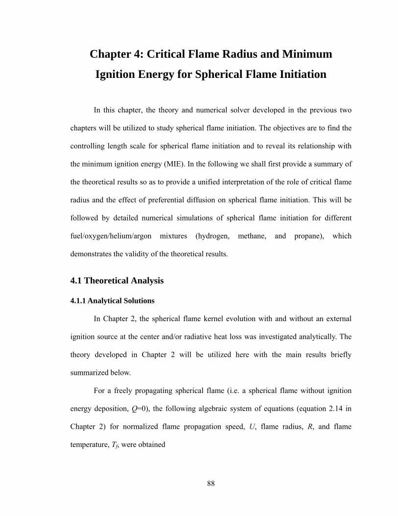
Chapter 4: Critical Flame Radius and Minimum
Ignition Energy for Spherical Flame Initiation
In this chapter, the theory and numerical solver developed in the previous two
chapters will be utilized to study spherical flame initiation. The objectives are to find the
controlling length scale for spherical flame initiation and to reveal its relationship with
the minimum ignition energy (MIE). In the following we shall first provide a summary of
the theoretical results so as to provide a unified interpretation of the role of critical flame
radius and the effect of preferential diffusion on spherical flame initiation. This will be
followed by detailed numerical simulations of spherical flame initiation for different
fuel/oxygen/helium/argon mixtures (hydrogen, methane, and propane), which
demonstrates the validity of the theoretical results.
4.1 Theoretical Analysis
4.1.1 Analytical Solutions
In Chapter 2, the spherical flame kernel evolution with and without an external
ignition source at the center and/or radiative heat loss was investigated analytically. The
theory developed in Chapter 2 will be utilized here with the main results briefly
summarized below.
For a freely propagating spherical flame (i.e. a spherical flame without ignition
energy deposition, Q=0), the following algebraic system of equations (equation 2.14 in
Chapter 2) for normalized flame propagation speed, U, flame radius, R, and flame
temperature, Tf, were obtained
88
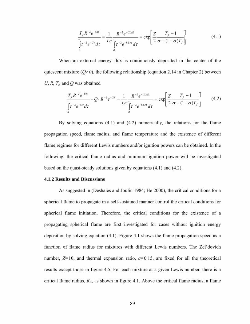
⎥⎥⎦
⎤
⎢⎢⎣
⎡
−+
−==
∫∫∞
−−
−−
∞−−
−−
f
f
R
ULe
ULeR
R
U
URf
TTZ
de
eRLe
de
eRT)1(
12
exp1
2
2
2
2
σσττττ ττ
(4.1)
When an external energy flux is continuously deposited in the center of the
quiescent mixture (Q>0), the following relationship (equation 2.14 in Chapter 2) between
U, R, Tf, and Q was obtained
⎥⎥⎦
⎤
⎢⎢⎣
⎡
−+
−==⋅−
∫∫∞
−−
−−−−
∞−−
−−
f
f
R
ULe
ULeRUR
R
U
URf
TTZ
de
eRLe
eRQde
eRT)1(
12
exp1
2
22
2
2
σσττττ ττ
(4.2)
By solving equations (4.1) and (4.2) numerically, the relations for the flame
propagation speed, flame radius, and flame temperature and the existence of different
flame regimes for different Lewis numbers and/or ignition powers can be obtained. In the
following, the critical flame radius and minimum ignition power will be investigated
based on the quasi-steady solutions given by equations (4.1) and (4.2).
4.1.2 Results and Discussions
As suggested in (Deshaies and Joulin 1984; He 2000), the critical conditions for a
spherical flame to propagate in a self-sustained manner control the critical conditions for
spherical flame initiation. Therefore, the critical conditions for the existence of a
propagating spherical flame are first investigated for cases without ignition energy
deposition by solving equation (4.1). Figure 4.1 shows the flame propagation speed as a
function of flame radius for mixtures with different Lewis numbers. The Zel’dovich
number, Z=10, and thermal expansion ratio, σ=0.15, are fixed for all the theoretical
results except those in figure 4.5. For each mixture at a given Lewis number, there is a
critical flame radius, RC, as shown in figure 4.1. Above the critical flame radius, a flame
89

can successfully propagate outward. On the other hand, no quasi-steady solution exists
below the critical flame radius. As shown in figure 4.1, the critical radius increases with
the Lewis number. This is because the propagating spherical flame has positive stretch
rate, and the highly curved spherical flame of small radius has high stretch rate, which
makes the flame weaker at higher Lewis numbers (Law 2006). It is seen that for mixtures
with small Lewis numbers (Le=0.5, and 0.7 in figure 4.1), the flame propagation speed
could be higher than the adiabatic planar flame speed (U>1.0). This is due to the
enhancement by positive stretch rate for flames with Lewis number less than unity (Law
2006).
Figure 4.1 also shows that the adiabatic flame ball radius (Zeldovich et al. 1985),
RZ, corresponding to zero propagating flame speed (U=0), increases with Lewis number.
It is found that for Le<1.35, the critical flame radius, RC, is equal to the flame ball radius,
RZ; while for Le>1.35, we have RC<RZ. Therefore, the stationary flame ball radius, RZ, is
not the minimum radius for the existence of propagating spherical flames in mixtures
with high Lewis numbers. This was first found by He (He 2000) and it was proposed that
the flame initiation is not controlled by the radius of stationary flame ball for mixtures
with high Lewis number (He 2000). As a result, the critical flame radius, RC, is proposed
to be the controlling length scale for spherical flame initiation, instead of the radius of
stationary flame ball, which is commonly considered to be the minimum radius below
which a spherical flame cannot propagate outwards (Deshaies and Joulin 1984;
Champion et al. 1986).
We now consider the case in which an external energy flux is deposited in the
center of a quiescent mixture and examine how the ignition power correlates with the
90

critical flame radius. The effect of ignition energy on the flame diagram and the transition
trajectory has been studied in Chapter 2 for mixtures with Lewis number around unity
(Le=0.8, 1.0, 1.2). In the present study, mixtures with large Lewis numbers are
investigated. Figure 4.2 shows the flame propagation speed as a function of flame radius
at different ignition power for mixtures with Le=2 and Le=2.5. For Q=0, only a C shaped
flame branch for U-R exists (which is also shown in figure 4.1 for Le>1.3), and there is a
critical flame radius, RC, at the turning point, and a flame ball radius, RZ, at U=0 (it is not
shown in figure 4.2 since RZ is larger than the upper bound of flame radius range). At low
ignition power, Q=0.5 for Le=2 and Q=1.0 for Le=2.5, there is a new branch (left branch)
of solution for U-R at small flame radii with the flame propagation speed decreasing
sharply to zero (flame ball solution). On the left branch, the maximum possible flame
radius is defined as the lower critical flame radius, RC−, and the flame ball solution is
defined as the lower flame ball radius, RZ−. The C shaped branch (right branch) is slightly
shifted to the left side due to the ignition power deposition. On the right branch, the
corresponding upper critical flame radius, RC+, and the upper flame ball radius, RZ
+ are
defined in the opposite way. It is seen that the left and right branches move towards each
other with increasing ignition power. Figure 4.2 shows that when the ignition power is
larger than a critical value (0.968 for Le=2 and 2.04 for Le=2.5), defined as the minimum
ignition power, Qmin, the two branches merge with each other, resulting in the new upper
and lower branches. Spherical flame can thereafter propagate outward along the upper
branch U-R correlation, and therefore successful spherical flame initiation is obtained.
The changes of the upper and lower critical flame radii and flame ball radii with
the ignition power are shown in figure 4.3. It is seen that the upper and lower flame ball
91

radii are both strongly affected by the ignition power. However, for the critical flame radii,
RZ− monotonically increases with Q, while RZ
+ remains almost constant at different Q.
The lower critical flame radius and the flame ball radius are almost the same. Here the
minimum ignition power is the power at which RC+=RC
−. In (Champion et al. 1986), the
minimum ignition power is defined as the power at which RZ+=RZ
−. From figure 4.3, it is
seen that the minimum ignition power defined according to RZ+=RZ
− (Q’min=1.048 for
Le=2 and Q’min=2.53 for Le=2.5) is higher than the Qmin defined based on the critical
flame radius (Qmin=0.968 for Le=2 and Qmin=2.04 for Le=2.5). Therefore, the minimum
ignition power is over-predicted in (Champion et al. 1986) based on the flame ball radius.
For mixtures with Lewis number less than 1.3, there is no C shaped branch for U-R and
the critical radius is the same as the flame ball radius. Therefore, the minimum ignition
power based on the critical flame radius is the same as that based on flame ball radius.
It is noted that the critical flame radius, RC+=RC
−, at the minimum ignition power
is nearly the same as the critical flame radius, RC, at the zero ignition power deposition
since RZ+ remains almost constant for different Q (figure 4.3). By comparing the critical
flame radius and flame ball radius, over-prediction of the minimum ignition power based
on flame ball radius instead of critical flame radius can be found. Figure 4.4 shows the
critical flame radius and flame ball radius for different Lewis numbers at Q=0. It is seen
that the critical flame radius strongly depends on the Lewis number and the flame ball
radius increases exponentially with Lewis number – the adiabatic critical flame radius is
it is more than one order larger for Le=2 than Le=1. As a result, the minimum ignition
power would be substantially over-predicted based on the flame ball radius for mixtures
with large larger Lewis numbers. Therefore, the critical flame radius should be
92

considered as the controlling length scale for a spherical flame initiation for mixtures
with Lewis number above a critical value, Le*=1.35. For Le<1.35, the critical radius is
the same as the flame ball radius, and the minimum ignition power can be correlated with
either the critical radius or the flame ball radius.
To see how the critical flame radius is correlated with the minimum ignition
power, the minimum ignition power, Qmin, and the cube of the critical flame radius, RC3,
for mixtures with different Lewis numbers (Le=1.4~2.5) and Zel’dovich numbers (Z=10,
13) are plotted in figure 4.5. Both Qmin and RC3 are shown to strongly depend on the
Lewis number. It is seen that the minimum ignition power varies almost linearly with the
cube of the critical flame radius, demonstrating a linear correlation: Qmin ~ RC3. Therefore
it is the critical flame radius that controls successful spherical flame initiation.
Furthermore, the minimum energy deposition for successful spherical flame initiation is
proportional to the cube of the critical flame radius instead of the flame thickness or the
flame ball radius.
The above results were obtained from theoretical analysis of spherical flames
based on the assumption of quasi-steadiness in the flame-front attached coordinate. The
shortcoming of this analysis is that the ignition energy deposition is modeled as a
boundary condition in the center; while under most realistic conditions it is resolved in
time and space. The steady-state energy deposition is employed in order to achieve an
analytical solution. However, this simplification does not prevent the model from
producing qualitatively correct results, as will be confirmed by results from unsteady
simulation. In the next section, energy deposition similar to practical ignition will be
utilized in detailed numerical simulation.
93

4.2 Numerical Validation
4.2.1 Numerical Specifications
In this section, the validity of the theoretical results presented in the previous
section is demonstrated by numerical simulations using detailed chemistry. A-SURF
developed in Chapter 3 is used here to simulate spherical flame initiation and
propagation.
Symmetric conditions at the center (r=0) and non-reactive, adiabatic condition at
the wall (r=1.0 m) are utilized in the simulation. At the initial state, the premixture is
assumed quiescent and homogeneous at 298 K and atmospheric pressure. Ignition is
achieved by energy deposition resolved in time and space and the following term is added
to the conservation equation of energy (Frendi and Sibulkin 1990),
⎪⎩
⎪⎨⎧
≥
<−=
ig
igigigigignit
tif
tifrr
rE
qτ
τπτπ
0
])(4
exp[3/4
63& (4.3)
where E is the total ignition energy, τig=200 μs, the duration of the source energy, and
rig=200 μm, the ignition kernel radius (large τig and rig are utilized here to prevent high
temperature, (>5000 K) in the center, above which the thermal and transport coefficients
are difficult to be evaluated). It is noted that the duration of the source energy and the
ignition kernel radius both affect the MIE, Emin (Lewis and Von Elbe 1961; Ronney 1994).
In the present study, fixed values of τig and rig specified above are utilized, and the
emphasis is on the correlation between the MIE and the critical flame radius, and the
preferential diffusion effect on spherical flame initiation.
Simulations utilizing detailed chemical mechanisms for different fuels (H2, CH4
and C3H8) have been conducted. To simulate the H2/O2/He/Ar and H2/air flames, the
94
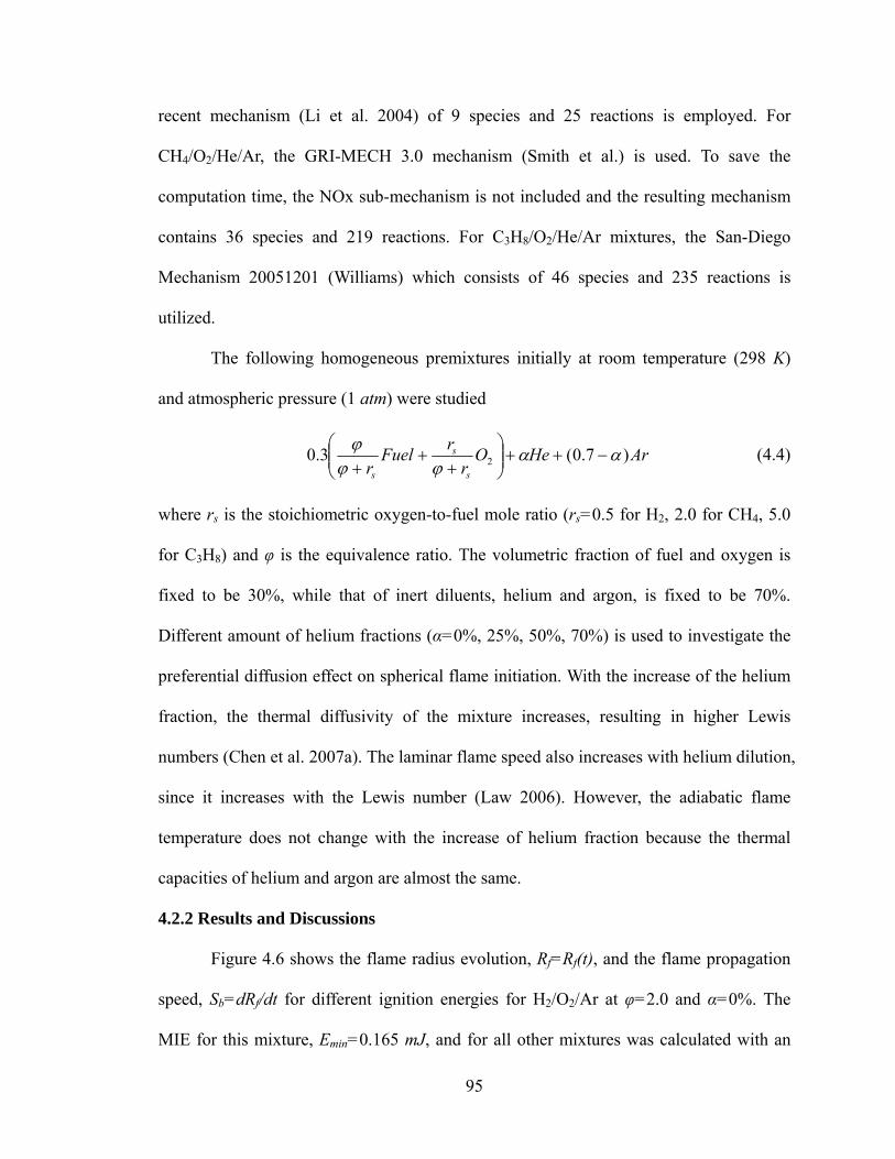
recent mechanism (Li et al. 2004) of 9 species and 25 reactions is employed. For
CH4/O2/He/Ar, the GRI-MECH 3.0 mechanism (Smith et al.) is used. To save the
computation time, the NOx sub-mechanism is not included and the resulting mechanism
contains 36 species and 219 reactions. For C3H8/O2/He/Ar mixtures, the San-Diego
Mechanism 20051201 (Williams) which consists of 46 species and 235 reactions is
utilized.
The following homogeneous premixtures initially at room temperature (298 K)
and atmospheric pressure (1 atm) were studied
ArHeOr
rFuelr s
s
s
)7.0(3.0 2 ααϕϕ
ϕ−++⎟⎟
⎠
⎞⎜⎜⎝
⎛+
++
(4.4)
where rs is the stoichiometric oxygen-to-fuel mole ratio (rs=0.5 for H2, 2.0 for CH4, 5.0
for C3H8) and φ is the equivalence ratio. The volumetric fraction of fuel and oxygen is
fixed to be 30%, while that of inert diluents, helium and argon, is fixed to be 70%.
Different amount of helium fractions (α=0%, 25%, 50%, 70%) is used to investigate the
preferential diffusion effect on spherical flame initiation. With the increase of the helium
fraction, the thermal diffusivity of the mixture increases, resulting in higher Lewis
numbers (Chen et al. 2007a). The laminar flame speed also increases with helium dilution,
since it increases with the Lewis number (Law 2006). However, the adiabatic flame
temperature does not change with the increase of helium fraction because the thermal
capacities of helium and argon are almost the same.
4.2.2 Results and Discussions
Figure 4.6 shows the flame radius evolution, Rf=Rf(t), and the flame propagation
speed, Sb=dRf/dt for different ignition energies for H2/O2/Ar at φ=2.0 and α=0%. The
MIE for this mixture, Emin=0.165 mJ, and for all other mixtures was calculated with an
95

error less than 3%. It is seen that there is a left branch of Sb-Rf, along which the spherical
flame could not successfully propagate outwardly when the ignition energy is less than
the MIE. Only when the ignition energy is above the MIE can a self-sustained
propagating flame be successfully initiated. The results are similar to the theoretical
results shown in figure 4.2, except the right and lower branches which could not be
calculated from the transient numerical simulation. It is noted that the critical flame
radius can not be defined in the same way as that in the quasi-steady theoretical analysis.
Figure 4.2 shows that the critical flame radius is almost the same flame radius at which
the minimum propagating speed occurs in case of the minimum ignition power
deposition. According to this, in numerical simulations, we define the critical flame
radius as the radius at which the minimum propagating speed occurs in case of MIE
deposition. In the diagram of flame radius evolution, Rf=Rf(t), the critical flame radius
occurs at the inflection point for E=Emin=0.165 mJ, which is RC=0.11 cm. Similar
results to those shown in figure 4.6 were also obtained from simulation (one-step
chemistry, constant thermal properties, and no thermal expansion) and experiments in
(Champion et al. 1986).
To investigate the preferential diffusion effect on spherical flame initiation,
numerical simulations on the initiation of H2/O2/He/Ar mixtures at different equivalence
ratios and different amounts of helium dilution were conducted. The burned Markstein
length, the MIE, and the critical flame radius of different H2/O2/He/Ar mixtures are
shown in figures 4.7, 4.8, and 4.9, respectively. The burned Markstein length, Lb, is
obtained from the linear extrapolation based on the plot of Sb-K, where the flame speed
relative to the burned gas, Sb=dRf/dt, and the flame stretch rate, K=(2/Rf)(dRf/dt),
96
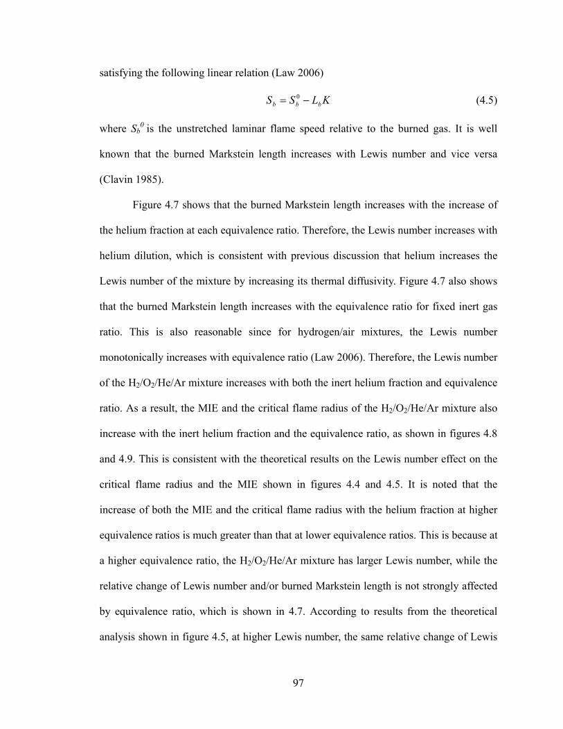
satisfying the following linear relation (Law 2006)
(KLSS bbb −= 0 4.5)
where Sb0 is the unstretched laminar flame speed relative to the burned gas. It is well
known that the burned Markstein length increases with Lewis number and vice versa
(Clavin 1985).
Figure 4.7 shows that the burned Markstein length increases with the increase of
the helium fraction at each equivalence ratio. Therefore, the Lewis number increases with
helium dilution, which is consistent with previous discussion that helium increases the
Lewis number of the mixture by increasing its thermal diffusivity. Figure 4.7 also shows
that the burned Markstein length increases with the equivalence ratio for fixed inert gas
ratio. This is also reasonable since for hydrogen/air mixtures, the Lewis number
monotonically increases with equivalence ratio (Law 2006). Therefore, the Lewis number
of the H2/O2/He/Ar mixture increases with both the inert helium fraction and equivalence
ratio. As a result, the MIE and the critical flame radius of the H2/O2/He/Ar mixture also
increase with the inert helium fraction and the equivalence ratio, as shown in figures 4.8
and 4.9. This is consistent with the theoretical results on the Lewis number effect on the
critical flame radius and the MIE shown in figures 4.4 and 4.5. It is noted that the
increase of both the MIE and the critical flame radius with the helium fraction at higher
equivalence ratios is much greater than that at lower equivalence ratios. This is because at
a higher equivalence ratio, the H2/O2/He/Ar mixture has larger Lewis number, while the
relative change of Lewis number and/or burned Markstein length is not strongly affected
by equivalence ratio, which is shown in 4.7. According to results from the theoretical
analysis shown in figure 4.5, at higher Lewis number, the same relative change of Lewis
97
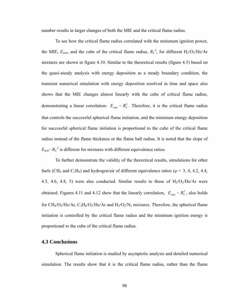
number results in larger changes of both the MIE and the critical flame radius.
To see how the critical flame radius correlated with the minimum ignition power,
the MIE, Emin, and the cube of the critical flame radius, RC3, for different H2/O2/He/Ar
mixtures are shown in figure 4.10. Similar to the theoretical results (figure 4.5) based on
the quasi-steady analysis with energy deposition as a steady boundary condition, the
transient numerical simulation with energy deposition resolved in time and space also
shows that the MIE changes almost linearly with the cube of critical flame radius,
demonstrating a linear correlation: . Therefore, it is the critical flame radius
that controls the successful spherical flame initiation, and the minimum energy deposition
for successful spherical flame initiation is proportional to the cube of the critical flame
radius instead of the flame thickness or the flame ball radius. It is noted that the slope of
E
3min ~ CRE
min−RC3 is different for mixtures with different equivalence ratios.
To further demonstrate the validity of the theoretical results, simulations for other
fuels (CH4 and C3H8) and hydrogen/air of different equivalence ratios (φ = 3, 4, 4.2, 4.4,
4.5, 4.6, 4.8, 5) were also conducted. Similar results to those of H2/O2/He/Ar were
obtained. Figures 4.11 and 4.12 show that the linearly correlation, , also holds
for CH
3min ~ CRE
4/O2/He/Ar, C3H8/O2/He/Ar and H2/O2/N2 mixtures. Therefore, the spherical flame
initiation is controlled by the critical flame radius and the minimum ignition energy is
proportional to the cube of the critical flame radius.
4.3 Conclusions
Spherical flame initiation is studied by asymptotic analysis and detailed numerical
simulation. The results show that it is the critical flame radius, rather than the flame
98

thickness or flame ball radius, that controls spherical flame initiation. The minimum
ignition energy for successful spherical flame initiation is shown to be proportional to the
cube of the critical flame radius. Furthermore, the preferential diffusion between heat and
mass (Lewis number effect) is found to play an important role in spherical flame
initiation. It is shown that the critical flame radius and the minimum ignition energy
increase significantly with the Lewis number. Therefore, for fuels with much higher
thermal diffusivity than fuel mass diffusivity, larger ignition energy is needed to initiate a
self-sustained propagating premixed flame.
99

Normalized flame radius, R
Nor
mal
ized
flam
epr
opag
atin
gsp
eed,
U
10-1 100 101 1020
0.4
0.8
1.2
1.6
Le=0.5
0.7
1.01.5
2 2.5
O
O OO
OO
Figure 4.1: Normalized flame propagation speed as a function of flame radius for
mixtures at different Lewis numbers (the critical flame radius for each case is denoted by
a circle at the corresponding minimum flame radius).
100

Normalized flame radius, R
Nor
mal
ized
flam
epr
opag
atin
gsp
eed,
U
0 10 20
10-3
10-2
10-1
100
Le = 2 .0
30
Q=00.5
Q=0.5
0.96
0.960.97
0.97
1
2
1
: RC-
: RC+
: RZ-
: RZ+
Normalized flame radius, R
Nor
mal
ized
flam
epr
opag
atin
gsp
eed,
U
0 10 20 30 40
10-2
10-1
100
Le = 2 .5
50
Q=01
Q=1
2
22.1
2.13
: RC-
: RC+
: RZ-
: RZ+
Figure 4.2: Normalized flame propagation speed as a function of flame radius at different
ignition power for mixtures with (a), Le=2; (b), Le=2.5.
101

Ignition power, Q
Flam
eba
llra
dius
RZ
,crit
ical
flam
era
dius
RC
0 1 2 3100
101
102
Qmin = 2.05
Qmin = 0.97
Le = 2.5
Le = 2.0 RC
RZ
RZ
RZ
RC
RC
+
-
+
+
+
-
RZ-
RC-
Figure 4.3: Change of upper and lower critical flame radii and flame ball radii with
ignition power.
Lewis number, Le
Crit
ical
flam
era
dius
/fla
me
ball
radi
us
0.5 1 1.5 2 2.510-1
100
101
102
RC
RZ
Figure 4.4: Critical flame radius and flame ball radius as functions of different Lewis
numbers.
102

Cube of critical flame radius, RC3
Min
imun
igni
tion
pow
er,Q
min
0 500 1000 1500 2000 25000
0.5
1
1.5
2
Z = 10
Cube of critical flame radius, RC3
Min
imun
igni
tion
pow
er,Q
min
0 500 1000 1500 2000 25000
0.5
1
1.5
2
Z = 13
2.0
1.4
1.6
1.7
1.8 = Le
1.9
1.51.4
2.5
2.0
1.9
1.8
1.71.6
1.5
Le = 2.1
2.3
2.4
2.2
Figure 4.5: Minimum ignition power and cube of critical flame radius for mixtures with
different Lewis numbers and Zel’dovich numbers.
103

Time, t (s)
Flam
era
dius
,Rf(c
m)
0 0.001 0.002 0.0030
0.1
0.2
0.3
0.4
ϕ = 2.00% He
E=0.2 mJ
0.18
0.17
0.165
Critical radius: RC = 0.11 cm
0.160.15
Flame radius, Rf (cm)
Flam
epr
opag
atin
gsp
eed,
Sb
(cm
/s)
0 0.05 0.1 0.15 0.2 0.250
50
100
150ϕ = 2.00% He
Critical radius: RC = 0.11 cm
E = 0.15,0.16,0.165,0.17,0.18,0.2 mJ
Figure 4.6: Spherical flame initiation for H2/O2/He/Ar mixtures at different ignition
energies: (a), temporal variation of flame radius; (b), flame propagation speed at each
radius.
104
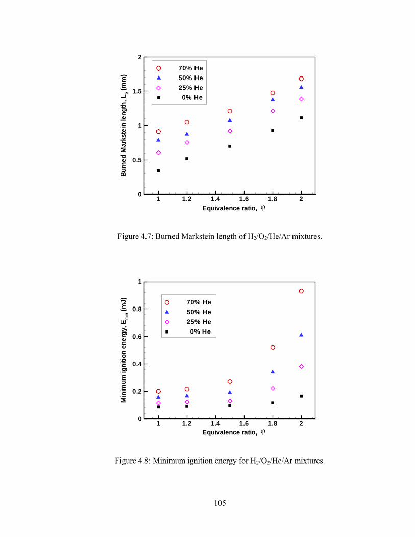
Equivalence ratio,
Bur
ned
Mar
kste
inle
ngth
,Lb
(mm
)
1 1.2 1.4 1.6 1.8 20
0.5
1
1.5
270% He50% He25% He0% He
ϕ
Figure 4.7: Burned Markstein length of H2/O2/He/Ar mixtures.
Equivalence ratio,
Min
imum
igni
tion
ener
gy,E
min
(mJ)
1 1.2 1.4 1.6 1.8 20
0.2
0.4
0.6
0.8
1
70% He50% He25% He0% He
ϕ
Figure 4.8: Minimum ignition energy for H2/O2/He/Ar mixtures.
105

Equivalence ratio,
Crit
ical
flam
era
dius
,RC
(mm
)
1 1.2 1.4 1.6 1.8 20
0.5
1
1.5
2
2.5
70% He50% He25% He0% He
ϕ
Figure 4.9: Critical flame radius of H2/O2/He/Ar mixtures.
Cube of critical flame radius, RC3 (mm3)
Min
imum
igni
tion
ener
gy,E
min
(mJ)
0 2 4 6 8 10 12 140
0.2
0.4
0.6
0.8
1= 1.5= 1.8= 2.0
ϕ
ϕϕ
12
3
4
1
2
3
4
1
2
3
4
Case vol.% He1 0%2 25%3 50%4 70%
Figure 4.10: Minimum ignition energy and cube of critical flame radius of H2/O2/He/Ar
mixtures
106

Cube of critical flame radius, RC3 (mm3)
Min
imum
igni
tion
ener
gy,E
min
(mJ)
0 1 2 3 4 50
0.5
1
1.5
H2
C3H8
CH4
He % vol. = 0, 25, 50,70 %
Stoichiometric Fuel+O2 = 30 % vol.Inert gas: He + Ar = 70 % vol.
Figure 4.11: Minimum ignition energy and cube of critical flame radius of different fuels
with different amount of He dilutions.
Cube of critical flame radius, RC3 (mm3)
Min
imum
igni
tion
ener
gy,E
min
(mJ)
0 10 20 30 400
0.5
1
1.5
2
2.5
H2/air
ϕ = 3, 4, 4.2, 4.4, 4.5, 4.6, 4.8, 5.0
Figure 4.12: Minimum ignition energy and cube of critical flame radius of rich H2/air
mixtures.
107

Chapter 5: On the Determination of Laminar Flame
Speed using Propagating Spherical Flames
In this chapter, the method of laminar flame speed measurement utilizing
propagating spherical flames in a confined bomb is investigated theoretically and
numerically. The emphasis is placed on how to improve the accuracy of flame speed
measurement. It is found that the accuracy is affected by different effects such as Lewis
number, ignition and unsteady flame transition, compression, and flame stretch. Rigorous
determination of flame speeds could be achieved by using techniques developed in this
chapter to correct these effects.
5.1 Introduction
As discussed in Chapter 1, tracking the evolution of an outwardly propagating
spherical flame in a confined bomb is currently the most preferred method for measuring
the laminar flame speed at high pressures. In this method, a quiescent homogeneous
combustible mixture in a closed chamber is centrally ignited by an electrical spark or a
laser beam which results in an outwardly propagating spherical flame (Lewis and Von
Elbe 1961; Rallis and Garforth 1980). The flame front history and/or the pressure rise
history are/is recorded during the experiment and subsequently related to the laminar
flame speed through theoretical models (described in the next two sections). Depending
on the bomb design and the pressure change, there are two different methods for flame
speed measurement by using the expanding spherical flames. The so-called constant
pressure method uses Schlieren photograph to view the flame front propagation history of
an expanding spherical flame in a large confined chamber or a pressure release
108

dual-chamber. There are two main advantages of this method. First, the propagating
flame surface is observed such that any distortion of the flame morphology from being
spherical or smooth can be detected; the former effect could occur for slow burning
flames due to buoyancy while the later from the development of flame front instabilities
especially those of cellular nature. Second, since the effect of the increase of the pressure
and temperature within the chamber on the flame speed is minimal during the early
stages, there exists a stage where the flame speed is purely a function of stretch —
allowing for extrapolation to zero stretch and determination of stretch behaviour.
Recently a great deal of effort has been devoted to obtaining accurate flame speeds
utilizing this method. For example, Kelley and Law (Kelly and Law 2007) suggested that
nonlinear extrapolation between the stretched flame speed and stretch rate should be used
for mixtures with Lewis numbers appreciably different from unity in order to obtain
accurate flame speed; Bradley et al. (Bradley et al. 2007) developed a method to correct
the flame speed enhancement due to flame wrinkling arising from hydrodynamic and/or
thermal-diffusive instabilities and measured laminar flame speed of lean hydrogen/air
mixtures; Burke et al. (Burke et al. 2008) demonstrated that the effect of flow field
deviation due to constant-pressure non-spherical chambers can significantly affect the
accuracy of flame speed measurements and the Flow-Corrected Flame Speed (FCFS) was
proposed to include the flow field deviation in order to improve the accuracy of flame
speed measurements.
The other experimental technique, the so-called constant volume method (Lewis
and Von Elbe 1961; Bradley and Mitcheson 1976; Metghalchi and Keck 1980; Hill and
Hung 1988) employs a fast-response pressure transducer to measure the chamber
109

pressure history during the propagation of an expanding spherical flame in a closed
thick-walled spherical vessel. Conversion of the reactants to hot products across the
flame front results in a rapid pressure rise and a consequent temperature rise in unburned
and burned gas. Therefore, this method has the advantage that the flame speed for a given
mixture over a wide range of temperatures and pressures can be obtained from a single
test (Metghalchi and Keck 1980). Recently, several improved theoretical models to relate
the experimentally measured pressure history to the instantaneous flame speeds have
been developed. Saeed and Stone (Saeed and Stone 2004) developed a multiple burned
gas zone model to allow for a more realistic temperature distribution within the burned
gas than the initially employed uniform temperature assumption. Metghalchi and
co-workers (Parsinejad et al. 2006) considered a variable-temperature central burned gas
core surrounded by a preheat zone, a uniform-temperature unburned gas shell, and a
thermal boundary layer at the wall in their model, and they accounted for different
sources of heat loss. Huzayyin et al.(Huzayyin et al. 2008) revealed that using different
models to relate the same pressure history (from the same experimental data) to the
laminar flame speed results in discrepancies up to 15% in the predicted flame speed. The
result indicates the importance of accurate models and the need to improve them further.
The objective of the present study is to investigate different effects such as
ignition and unsteady transition, compression, and flame stretch on the accuracy of
laminar flame speed measurements using propagating spherical flames and to develop
new methods to obtain more accurate flame speeds in a broader experimental range by
correcting these effects. For the constant pressure method, the assumptions such as the
linear relationship between the stretched flame speed and stretch rate, negligible effects
110

due to ignition and unsteady transition, and zero burned gas velocity will be investigated.
For the constant volume method, the stretch effect on the measured flame speed will be
studied. For both methods, the validity of the theoretical models and the improvement in
the accuracy of measured flame speed will be demonstrated by numerical simulations
using detailed chemistry for different fuels (hydrogen, methane, and propane). In this
study, detailed numerical simulations instead of experimental measurement were utilized
because: 1), the compression induced flow field (which is difficult to measure in
experiments) can be readily obtained from simulation and thus it is compared with the
theoretical prediction; and 2), other effects such as radiative loss (which always exists in
experiments) can be included/excluded in simulations in order to isolate the effects of
interest.
5.2 Constant Pressure Method
For the outwardly propagating spherical flame, the flame front, Rf=Rf(t), has a
propagation velocity, dRf/dt. If the radial flow velocity is defined positive in the outward
direction, and the flame front is assumed to be infinitely thin, the velocity of the flame
front must be subtracted from that in the mass flow balance through the flame front
(Peters 2000)
)()(dt
dRU
dtdR
U fbb
fuu −=− ρρ (5.1)
where ρ and U are density and flow velocity caused by thermal expansion across the
flame front, respectively. The subscripts u and b refer to parameters for unburned and
burned mixtures, respectively. At the flame front, the kinetic balance between the
propagation velocity (dRf/dt), flow velocity (Uu), and flame speed with respect to the
111
unburned gas (Su), is
uuf SU
dtdR
+= (5.2)
Similarly, the kinetic balance with respect to the burned mixture is
bbf SU
dtdR
+= (5.3)
According to the mass conservation given by equation (5.1), we have
bu aSS = (5.4)
where a=ρb/ρu is the density ratio. Note that both Su and Sb are laminar flame speeds
under finite stretch rate. For outwardly propagating spherical flames, the flame stretch
rate is (Clavin 1985)
dtdR
RdtdA
AK f
f
21== (5.5)
where A=4πRf2 is the surface area of the flame front. The above flame stretch rate could
be separated into two components: one due to the strain rate and the other due to the
flame curvature (Bradley et al. 1996; Groot et al. 2002). Therefore, separate effects due to
strain rate and curvature on flame speed can be studied (Bradley et al. 1996; Groot et al.
2002). However, it has been shown that the Markstein length with respect to the stretch
due to strain rate is not unique while that with respect to the stretch rate given by
equation (5.5) is unique (Groot et al. 2002). Moreover, in most of the previous
experimental measurements (Brown et al. 1989; Dowdy et al. 1990; Tseng et al. 1993;
Aung et al. 1997; Hassan et al. 1998; Tse et al. 2000; Rozenchan et al. 2003) the stretch
rate defined by equation (5.5) was used. Therefore, it is also used in the present study and
the separate effects by strain rate and curvature is not studied here. For weakly stretched
112
flames, a linear relationship between the stretched flame speed and the stretch rate exists
that is quantified by a burned gas Markstein Length, Lb (Clavin 1985)
KLSS bbb −= 0 (5.6)
where Sb0 is the unstretched flame speed with respect to the burned mixture. The
unstretched laminar flame speed with respect to the unburned mixture, Su0, is given
through mass conservation
00bu aSS = (5.7)
By substituting equations (5.4) and (5.7) into (5.6), we have
KaLSS buu −= 0 (5.8)
From equations (5.3) and (5.4), the stretched flame speed, Su, is given by
bf
u aUdt
dRaS −= (5.9)
In all previous studies utilizing the constant pressure method, data reduction was
performed only for “small” pressure change and the burned gas is assumed to be
quiescent (Ub≈0). As a result, the moving velocity of the experimentally visualized flame
front is the burned flame speed, and from equation (5.9) we have
)/( dtdRaS fu ≈ (5.10)
Therefore, according to equation (5.8), the unstretched laminar flame speed, Su0,
and burned gas Markstein Length, Lb (or the unburned gas Markstein Length, Lu=aLb),
can be obtained from the linear extrapolation based on the plot of Su-K, where Su and K
are calculated from the flame front history, Rf=Rf(t), according to equations (5.10) and
(5.5), respectively. It should be noted that the flame front is assumed to be infinitely thin
in the above discussions. The effect of finite flame thickness, discussed in (Bradley et al.
113
1996; Bradley et al. 1998; Gu et al. 2000; Groot et al. 2002), is not included here.
The constant pressure method discussed above is based on the following
assumptions: linear relationship between the stretched flame speed and stretch rate,
negligible effects due to ignition and unsteady transition, zero burned gas velocity, and
negligible radiative loss. In the following, the conditions under which these assumptions
hold and the corrections for circumstances that these assumptions do not hold will be
investigated.
5.2.1 Validity of the Linear Relationship between Flame Speed and Stretch
To investigate under what conditions the stretched flame speed changes linearly
with the stretch rate, the theory for propagating spherical flames presented in Chapter 2 is
utilized here. By neglecting radiative loss, the relationship between the normalized flame
radius, R=Rf/δ, and the normalized flame speed, U=Sb/Sb0, can be expressed as
⎥⎥⎦
⎤
⎢⎢⎣
⎡
−+
−==⋅−⋅
∫∫∞
−−
−−−−
∞−−
−−
f
f
R
ULe
ULeRUR
R
U
UR
f TTZ
de
eRLe
eRQde
eRT)1(
12
exp1
2
22
2
2
σσττττ ττ
(5.11)
where Tf, Q, and Z are, respectively, the normalized flame temperature, ignition power at
the center, and Zel’dovich number, which are defined in Chapter 2. Equation (5.11) is
valid for flames at both small and large radii. Hereafter, we refer to it as the detailed
model (DM).
For spherical flames of large radii (R>>1), the detailed model reduces to the
simplified model (SM)
)11(2)11()2ln()2( −−−=++LeRLeR
ZR
UR
U (5.12)
For weakly stretched flames, the stretched flame speed is close to the adiabatic
114

unstretched flame speed (i.e. U=1+ε with ε<<1). In this limit, equation (5.12) reduces to
the linear model (LM)
KaMaU ⋅−= 1 (5.13)
where Ka=2U/R=Kδ/Su0 is the Karlovitz number and Ma=Le-1-(Z/2)(Le-1-1) the
Markstein number, which is the same as that derived for premixed counterflow flame
(Law 2006).
The linear relationship, equation (5.6) or (5.8), utilized for linear extrapolation for
constant pressure method, is based on the LM given by equation (5.13). To find under
which conditions the LM works well, the normalized flame speed predicted as a function
of flame radius and the Karlovitz number (in figures 5.1(b) and 5.5(b), Ka=2U/(σR) is
used since the propagating speed, thus the flame stretch, is 1/σ times of the laminar flame
speed, Su0, to the zeroth order) by DM, SM, and LM for Z=10, σ=0.15 and Le=0.5, 1.0,
2.0 is shown in figure 5.1. It is observed that SM and LM agree well with DM only for
large flame radius. In addition, the difference among the prediction from DM, SM, and
LM strongly depends on the Lewis number. Figure 5.1(b) reveals that for each Lewis
number, there is a critical Karlovitz number above which the spherical flame does not
exist, due to the quenching caused by the combined effects of flame curvature and stretch.
The maximum Karlovitz number for Le=2 is much smaller than that for Le=0.5 and 1.0,
indicating that small spherical flames does not exist for large Lewis numbers. Finite
flame curvature always decreases the flame speed (equation 5.12). However, the effect of
flame stretch on flame speed depends strongly on the Lewis number derivation from
unity (Law 2006). As a result, the critical Karlovitz number, denoted by the turning points
in figure 5.1(b), decreases significantly with increasing Lewis number. As will be shown
115

later, this conclusion plays an important role in determining the experimental data range
for flame speed measurement.
Figure 5.2 shows the critical flame radius above which the relative discrepancies
between LM and DM and between SM and DM are less than 5%. It is seen that the
critical flame radius of SM is much smaller than that of LM for a given Lewis number,
which is consistent with the fact that the SM is more comprehensive than the LM (SM is
based on the assumption of large flame radius; while LM is based on the assumption of
large flame radius as well as small stretch rate). The nonmonotonic change of the critical
flame radius with Lewis number is due to the fact that the absolute value of the Markstein
length becomes smallest when Le is close to a critical value which is slightly less than
unity (Law 2006).
By comparing the three different models of DM, SM and LM given by equations
(5.11-5.13), we obtain the critical flame radius above which the linear or non-linear
relationship between the stretched flame speed and stretch rate is satisfied. This critical
flame radius can be used as a guide to choose the experimental data range for flame speed
measurement by using either linear or nonlinear fitting approaches based on equation
(5.11) or (5.12). Since the critical flame radius changes greatly with Lewis number, for
mixtures such as rich hydrogen/air or lean propane/air with Lewis numbers greatly
different from unity, the lower flame radius bound RfL should be specified above the
critical radius so that the linear (based on LM) or nonlinear (based on SM) extrapolation
can be carried out.
5.2.2 Effects of Ignition and Unsteady Transition
The above theoretical analysis is based on the quasi-steady assumption, with the
116
effects of ignition and unsteadiness are neglected. In order to study the effects of
unsteady flame evolution at different ignition energies, A-SURF (1D) described in
Chapter 3 is used to simulate outwardly propagating spherical flames. Detailed chemistry
is included in the simulation: for H2/air flames, the recent mechanism of 9 species and 25
reactions developed by Li et al. (Li et al. 2004) is employed. The spherical chamber
radius is set to be R0=100 cm and the flame trajectory data with flame radius less than 5
cm are utilized. Therefore, both the pressure increase (<1‰) and the
compression-induced flow effect described in the next section are negligible. The flame is
initiated by a small hot pocket of burned product surrounded by fresh mixture at the room
temperature and pressure (T0=298 K, P0=1 atm). The size of the hot pocket, Rh, is
between 0.9 mm and 2.0 mm, which changes with the equivalence ratio of H2/air. For
very rich cases (φ=5.0 or 5.5), which have large Lewis numbers, a larger hot pocket is
needed to obtain a propagating spherical flame (Chen et al. 2008b). In order to examine
the effect of ignition energy on flame trajectories, at a fixed equivalence ratio, three
different hot pocket sizes, Rh, 1.2Rh, 1.4Rh, were adopted to mimic the experiments with
different ignition energies. The position of the flame front, Rf, is defined as the position of
maximum heat release rate and the flame speed is calculated from the flame front history,
i.e. Sb=dRf/dt.
The propagating spherical H2/air flames at different equivalence ratios (φ=0.5, 1.0,
2.0, 3.0, 3.5, 4.0, 4.5, 5.0, 5.5) and different ignition hot pocket sizes are simulated.
Figure 5.3 shows the flame speed with respect to the burned mixture, Sb, as a function of
the flame radius, Rf, and flame stretch rate, K. The results show that the initial unsteady
flame transition and different ignition energies (hot pocket sizes) lead to different flame
117
speed trajectories. Only above a critical flame radius, Rc, which is denoted by the open
circles in figure 5.3, does the flame speed trajectory become independent of the ignition
energy and converge to a low-dimensional manifold. With the increase of equivalence
ratio, this critical flame radius increases dramatically. For φ=4.5, the critical radius is
even larger than 0.8 cm, which lies within typical experimental data ranges utilized for
extrapolation of flame speed. For example, lower flame radius bounds, RfL, of 0.5 cm or
0.6 cm are often employed (Kwon et al. 1992; Tseng et al. 1993; Bradley et al. 1996; Tse
et al. 2000; Farrell et al. 2004). Therefore, care is needed to fit the experimental data for
flame speed measurements of mixtures with large Lewis numbers. Moreover, figure 5.3(b)
shows that for flame radii larger than the critical radius (i.e. stretch rates less than the
critical stretch rate, which are marked by the open circles), Sb changes linearly with K,
except for very small Lewis numbers (the lean case at φ=0.5). As a result, for these
conditions, the linear extrapolation can be utilized to obtain unstretched flame speed.
For H2/air flames, the critical radius from present simulations and the effective
Lewis number based on contributions from both reactants in (Joulin and Mitani 1981;
Law 2006) are shown in figure 5.4. The critical radius is shown to change
non-monotonically with the equivalence ratio and is smallest for φ=2, which corresponds
to the largest laminar flame speed and the smallest flame thickness. The nonmonotonic
trend between the critical radius and equivalence ratio is similar to that between the flame
thickness and equivalence ratio. This is caused by the fact that the duration of initial
flame transition period (which is proportional to critical radius) strongly depends on the
flame thickness.
In order to understand the cause for the strong flame trajectory dependence on the
118

ignition energy and Lewis number, the dependence of normalized flame speed on the
Karlovitz number (Ka=Kδ/Su0) of spherical H2/air flames is shown in figure 5.5(a). The
maximum Karlovitz number changes greatly with the equivalence ratio, or more
accurately, with the Lewis number. This predicted dramatic change of the maximum
Karlovitz number is consistent with the theoretical prediction shown in figure 5.1(b). To
show the effects of ignition energy, the theoretical results for a mixture with Le=2 are
shown in figure 5.5(b) for comparison. Theory predicts that the ignition energy does not
affect the flame trajectories above the turning point of maximum Karlovitz number. This
is due to the fact that energy deposition is treated as a boundary condition at the center
and the unsteadiness is not included in the asymptotic theory. However, contrary to the
theory, figure 5.5(a) shows that there is a strong unsteady effect near the maximum
Karlovitz number. Due to the unsteady effect, the flame speed trajectory depends on the
ignition energy. For φ=4.5, the simulations reveal that, at large Karlovitz numbers, flames
initiated by large ignition energies have large flame speeds. However, near the maximum
Karlovitz number, flames initiated by smaller ignition energies have larger flame speed.
This new phenomenon is called “flame speed reverse”, which originates from the
unsteady flame evolution near the adiabatic extinction limit (the point of maximum
Karlovitz number in figures 5.5(a) and 5.1(b)). Because of the existence of the flame
speed reversal at large Lewis numbers, neither nonlinear fitting nor linear fitting of
experimental data including the flame speed reverse period for flame speed determination
is correct. Ignition energy and transient flame evolution significantly affect the flame
trajectories and thus must be considered.
For flame radii larger than the critical radius (figure 5.3), flame speed becomes
119

only dependent on the Karlovitz number. The critical radius above which the unsteady
flame transition ends can be found by observing the change of the flame thickness during
flame propagation. Figure 5.6 shows the history of flame thickness (defined as the
distance between the cold, T=400 K, and hot, T=1000 K, sides of the flame) during flame
propagation for H2/air at φ=4.5 initiated from three different ignition hot pocket sizes
(cases a, b, c, marked also in figures 5.3 and 5.5). The results indicate that there is a
significant change in the flame thickness during the initial period of unsteady flame
transition. The substantial thickening of the flame initiated by the smallest ignition energy
before it reaches the maximum Karlovitz number is the cause of the flame speed reversal.
After the transition period, the flame thickness is almost constant and the three lines
merge together onto the low-dimensional manifold for Rf>Rc. The change of flame
thickness during flame propagation clearly demonstrates the effect of unsteadiness on the
flame trajectory. In addition to the above results obtained under atmospheric conditions,
numerical simulations of H2/air flames at elevated pressures have also been conducted
(figure 5.7). It is found that the flame speed reversal effect also exists at high pressures
and that the critical radius decreases with pressure.
Therefore, the ignition energy has a significant impact on the flame trajectory and
the unsteady flame transition causes a flame speed reversal phenomenon, which greatly
narrows the experimental data range for flame speed extrapolation. Experiments (Chen et
al. 2008a) on outwardly propagating spherical H2/air flames have been conducted to
validate the above theoretical and numerical results about Lewis number and
ignition/unsteadiness effects.
120

5.2.3 Effect of Compression
In the previous section, the flow compression effect due to the interaction between
the burned gas thermal expansion and the chamber walls is neglected and the flow
velocity in the burned gas is assumed to be zero (Ub≈0). As will be shown in this section,
neglecting the compression-induced flow velocity, Ub, even for a small pressure increase
could significantly reduce the accuracy of the flame speed measurements. In the
following, an analytical expression of Ub will be derived and a Compression-Corrected
Flame Speed (CCFS) will be presented.
The mass conservation in the spherical bomb gives
0mmm ub ≡+ (5.14)
dtdmdtdm bu // −= (5.15)
in which mb and mu are, respectively, the mass of burned and unburned gases and m0 is
the total mass which does not change with time. According to the definition of flame
speed, we have
uufu SRdtdm ρπ 24/ −= (5.16)
Based on the assumptions that the spherical flame is thin and the temperature is
uniform in the burned gas region, we have
bfb Rm ρπ 3)3/4(= (5.17)
By further assuming that the burned gas behaves as an ideal gas and that the compression
is isentropic during the flame propagation, we have
PdPd bb γρρ // = (5.18)
where γ is the ratio of heat capacities, and P is the pressure which is nearly uniform in a
closed chamber (Lewis and Von Elbe 1961). Substituting equations (5.15) and (5.17) into
121
(5.16) and using the above isentropic relationship, one obtains (Lewis and Von Elbe
1961; Bradley and Mitcheson 1976; Hill and Hung 1988)
dtdP
PR
adt
dRaS ff
u γ3+= (5.19)
By comparing equations (5.9) and (5.19), the flow velocity of the burned gas
behind the flame front is
dtdP
PR
U fb γ3
−= (5.20)
The pressure and its rate of change in equation (5.20) can be either measured directly in
experiments or calculated from the flame front history obtained from the Schlieren
images according to the following relationship (Bradley and Mitcheson 1976)
3/1/10
00
)(1 ⎥⎦
⎤⎢⎣
⎡−−
−= γ
PP
PPPP
RR
e
ef (5.21)
where P0 and Pe are the initial and final chamber pressures, respectively, and R0 is the
radius of a spherical chamber (which is the equivalent radius, R0=(3V/4π)1/3, for a
non-spherical chamber of volume V).
With the increase of pressure, the unburned gas temperature, Tu, will also increase
so that the density ratio, a, is not a constant but a function of Tu
1)/1(/)( −Δ+== uaduu TTTTTa (5.22)
where ΔT is the temperature increase caused by chemical heat release and it can be
calculated from thermodynamic data. Assuming the unburned gas is compressed
isentropically, Tu can be calculated from the pressure which can be evaluated from the
flame front history according to equation (5.21), Tu=T0(P/P0)(1-1/γ). Then Tu and thus
a=a(Tu) can also be calculated from the flame front history.
122

Therefore, the compression-induced flow velocity, Ub, can be evaluated from the
flame front history by using equations (5.20) and (5.21). As a result, flame speed
extrapolated by using equation (5.9) instead of (5.10) is more accurate due to the
inclusion of the compression effect. The unstretched flame speed, Su0, obtained by the
linear extrapolation of Su given by equations (5.9), (5.20) and (5.21), is called the
Compression-Corrected Flame Speed (CCFS).
To show the improvement of the accuracy in flame speed measurement by CCFS,
A-SURF is used to simulate propagating spherical flames in a closed chamber for
different fuels (H2, CH4 and C3H8). Detailed chemistry is included in simulation, as
specified previously in Section 4.2.1 for the H2/air, CH4/air, and C3H8/air flames.
In all the simulations, the spherical chamber radius is set to be R0=6 cm. All the
results in the following parts are presented in terms of flame radii normalized by the
chamber size (Rf/R0). Therefore the same conclusions still hold for the cases using other
chamber sizes (normalized results from simulations with R0=12 cm show quantitatively
similar results as those with R0=6 cm). The flame is initiated by a small hot pocket (~1
mm in radius) of burned products surrounded by fresh mixture at room temperature and
pressure (298 K, 1 atm). At the inner and outer boundaries, r=0 and r=R0, respectively,
zero-gradient conditions are enforced. The effects of ignition and unsteadiness discussed
previously are excluded and only the data for flame radii larger that 6 mm are used to
calculate the flame speed in this section.
For the constant pressure method, similar to the Schlieren imaging in the
experiments, the flame front history, Rf=Rf(t), from the numerical simulation is used to
calculate the flame speed. In the simulation, the position of flame front is defined as the
123

position of maximum heat release It was pointed out that the level of contours chosen to
track the flame front might affect the flame front propagating speed (Bradley et al. 1996).
However, this second-order effect is important only for very lean or rich pre-mixtures
which have much thicker reaction zones. The chamber pressure can be either obtained
from simulation or calculated from flame front history by solving equation (5.21). The
difference between the pressures obtained from those two methods is negligible. The
compression-induced flow velocity, Ub, is defined as the flow velocity at the position
where 99.9% of the chemical heat is released.
Figure 5.8 shows the change of the flow field during flame propagation. There is a
velocity jump at the flame front induced by thermal expansion resulted from chemical
heat release in the flame reaction zone. The product and unburned mixture are ‘expanded’
inwardly and outwardly, respectively. When the relative flame radius is small, the
velocity of burned gas is negligible and thus the assumption of zero burned gas velocity
is reasonable. However, as shown in figure 5.8, the velocity of burned gas continuously
increases during the flame propagation. Therefore, without including the movement of
the burned gas, the flame speed would be under-predicted. This is further shown in
figures 5.9~5.11, which are results from the same simulation of the outwardly
propagating spherical stoichiometric CH4/air flame. Figure 5.9 shows the normalized
compression-induced flow velocity of the burned gas behind the flame front, aUb/SL0, as a
function of normalized flame radius or relative pressure increase. The results from the
theoretical relations given by equations (5.20) and (5.21) agree well with those from the
simulation. Note that to the zeroth order of accuracy, we have Su≈SL0 (Su is the stretched
flame speed while SL0 is the planar unstretched flame speed). Therefore, according to
124

equations (5.9) and (5.10), aUb/SL0 is the relative error in evaluating the stretched flame
speed, Su, caused by neglecting the compression-induced flow, Ub. The results indicate
that for normalized flame radius Rf/R0 larger than 0.4, the error will be greater than 5%.
Thus, for larger flames, in order to derive accurate flame speeds from experimental
measurements, the flow compression effect must be considered. As will be shown in
figure 5.11, this error is further amplified during the linear extrapolation process to obtain
the unstretched flame speed. Note that when the normalized flame radius Rf/R0 is less
than 0.5, the relative pressure increase is below 18% and the increase of the temperature
of unburned mixture is less than 12 K. The resulting change of the laminar flame speed is
less than 1% and thus is negligible.
The flow compression effect on the stretched flame speed is further demonstrated
in figure 5.10, in which different methods are employed to calculate the stretched flame
speed, Su. The normalized stretch rate is defined as K’=Kδ/SL0, with δ=0.2 mm and
SL=37.2 cm/s being the unstretched adiabatic laminar planar flame thickness and flame
speed, respectively. Figure 5.10 reveals that if the effect of flow compression is not
considered, i.e. Su=a(dRf/dt), Su decreases with increasing flame size when Rf/R0>0.3.
This is due to the fact the flame front propagating speed is reduced by the
compression-induced flow (note that Ub is negative as shown in figure 5.9). The rapid
decrease of the flame speed at large flame radii (or small stretch rate) renders the linear
extrapolation to zero stretch rate inaccurate. Therefore, in order to obtain an accurate
unstretched flame speed (Su0) from the linear extrapolation of Su-K according to equation
(5.8), an upper bound, RfU, must be chosen to make RfU/R0<0.3 such that the effect of the
compression-induced flow is prevented. Otherwise the flame speed will be
125

under-predicted. For a small combustion chamber of R0=6 cm, the RfU that satisfies
RfU/R0<0.3 is 1.8 cm. As such, the flame radius range, [RfL, RfU], for which the constant
pressure relations are accurate, is [0.6 cm, 1.8 cm]. This flame radius range might be too
narrow for accurate linear extrapolation. Therefore, the compression-induced flow
velocity, Ub, should be considered to extend the upper bound, RfU. Figure 5.10 shows that
when the flow velocity, Ub, is considered, i.e. Su=a(dRf/dt-Ub), without including the
temperature change, Su will monotonically increase during flame propagation (increase of
Rf) until Rf/R0>0.52. Therefore the upper bound, RfU, is extended more than 70% by
considering the compression-induced flow velocity, Ub. The decrease of Su for Rf/R0>0.52
is caused by the change of density ratio, a, with the increase of the unburned gas
temperature, Tu, as mentioned previously, and thus the density ratio is a function of Tu
instead of being constant, i.e. a=a(Tu), which is given by equation (5.22). Accordingly,
figure 5.10 shows that if the change of density ratio is also considered, i.e.
Su=a(Tu)·(dRf/dt-Ub), Su monotonically increases during the entire flame propagation
process as is expected for a positive Markstein length mixture and a flame with
increasing Tu. It should be noted that when the pressure increase is small ((P-P0)/P0<2%
or Rf/R0<0.25), the compression induced flow, Ub, is negligible and thus the stretched
flame speeds calculated from all three methods are almost the same. However, the two
CCFS methods yield linear relationships with stretch rate, as predicted by theory, for
larger spans of data.
To reveal how the choice of the flame radius range affects the measured laminar
flame speed by the flow compression effect, the accuracy of the unstretched flame speed
with and without the flow compression correction using different flame radii ranges, [RfL,
126
RfU], are shown in figure 5.11. The unstretched flame speed, Su0, is extrapolated from the
plot of Su-K according to equation (5.8) and SL0=37.2 cm/s is the laminar flame speed of
the unstretched planar flame at the room temperature and pressure obtained from the 1-D
planar flame simulation. When the compression effect is neglected, i.e. Su=a(dRf/dt),
figure 5.11 shows that the flame radius range affects greatly the extrapolated unstretched
flame speed, Su0, with the increase of the upper bound of the flame radius, Su
0,
significantly under-predicted (by more than 20%). This large discrepancy reveals that the
flow compression effect on flame speed is magnified by the linear extrapolation to zero
stretch rate. However, when the compression induced flow velocity, Ub, is considered and
the CCFS is employed, i.e. Su=a(dRf/dt-Ub), the discrepancies between the extrapolated
unstretched flame speed, Su0, using different flame radii ranges are all below 5%.
Therefore significant improvement in the accuracy of flame speed measurements is
achieved using the CCFS, which considers the compression-induced flow. A typical data
range utilized in previous experiments is [1.0 cm, 2.5 cm]. For chambers of radius larger
than 10 cm (Brown et al. 1989; Dowdy et al. 1990; Tseng et al. 1993; Aung et al. 1997;
Bradley et al. 1998; Gu et al. 2000), the accuracy of flame speed measurements
neglecting the compression effect is below 5% according to figure 5.11. However, these
experiments are for measurements below 5 atmospheres. For measurements of flame
speed at high pressures (above 10 atmosphere), smaller chamber should be used for
safety issues and only flames of small size can be used because hydrodynamic instability
and/or thermal diffusive instability, making flame front wrinkled, will occur earlier at
higher pressures (Rozenchan et al. 2003). When a chamber of 5 cm in radius is used, to
use the data range of [1.0 cm, 2.5 cm] will result in errors of 15%. Only when the CCFS
127
is employed, the error becomes less than 5%.
Figure 5.12 shows the accuracy of the unstretched flame speed for stoichiometric
H2/air and C3H8/air flames, respectively. The results are similar to those of CH4/air
mixtures. All the results demonstrate that: 1), the compression-induced flow and flame
radius range have significant impacts on the accuracy of the measured flame speed; 2),
the compression-induced flow can be accurately predicted by the analytical correlation
given by equations (5.20) and (5.21); 3), the accuracy of the flame speed measurements
can be greatly improved using the CCFS; and 4), for high pressure experiments using
small chambers, CCFS should be utilized to obtain accurate flame speed.
5.3 Constant Volume Method
The constant volume method also uses a spherical vessel with central ignition.
However, it calculates the flame speed based on the pressure history, P=P(t), recorded
after the flame has grown to a sufficiently large size so that the pressure variation is
evident. Details of theoretical analysis on this method can be found in (Lewis and Von
Elbe 1961; Bradley and Mitcheson 1976; Hill and Hung 1988) and are only briefly
described below.
The constant volume method is based on the following assumptions (Hill and
Hung 1988): the flame is thin, smooth, and spherical; the pressure is spatially uniform;
the constituents of the burned and unburned gases behave as ideal gases; the dissociation
products are in equilibrium; the unburned gas is compressed isentropically; and buoyancy
effects are negligible. These assumptions allow for the calculation of properties of the
burned and unburned gases in a constant volume combustion process.
First, we define the mass fraction of burned gas, x, as
128

00 /1/ mmmmx ub −== (5.23)
where the burned mass is given by equation (5.17). The unburned and total masses are
given by the following two equations, respectively,
ufu RRm ρπ )()3/4( 330 −= (5.24)
0300 )3/4( uRm ρπ= (5.25)
where ρu0 is the initial mixture density. According to the isentropic assumption we have
γ
ρρ /10
0
)(PP
u
u = (5.26)
From equations (5.14), (5.16), (5.24-26), the following expressions for flame
speed, Su, can be obtained
dtdx
PP
RRS
fu
γ/102
30 )(
3= (5.27)
3/1/10
0
))(1(1 ⎥⎦⎤
⎢⎣⎡ −−= γ
PPx
RR f (5.28)
The above equations describe essentially the technique for determining the
laminar flame speed from the pressure history (Lewis and Von Elbe 1961; Bradley and
Mitcheson 1976; Hill and Hung 1988). Equilibrium calculations (Metghalchi and Keck
1980; Takizawa et al. 2005) at the constant volume condition are carried out to obtain the
relationship of P with x, γ, and the burned and unburned gas temperatures, Tb and Tu.
These relationships are then applied to the experimentally measured pressure, P, and
finally the flame speed, Su, is obtained by solving equations (5.27) and (5.28). Detailed
descriptions are given in (Metghalchi and Keck 1980; Takizawa et al. 2005). For
simplicity, the commonly employed assumption of a linear relationship between the mass
129

fraction of the burned gas and pressure rise is employed (Lewis and Von Elbe 1961;
Bradley and Mitcheson 1976; Hill and Hung 1988),
)/()( 00 PPPPx e −−= (5.29)
The validity of this assumption is confirmed by detailed numerical simulation in
the next sub-section (figure 5.14b). Substituting equation (5.29) into (5.27) and (5.28),
the relationship in (5.21) is readily obtained and the flame speed is given by
dtdP
PP
PPRRR
S u
efu
γ/10
0
200 )()(
1)(3 −
= (5.30)
Therefore, from the pressure history P=P(t), the flame position Rf can be obtained
according to equation (5.21) and the stretched flame speed Su can be evaluated by using
equation (5.20).
5.3.1 Effect of Stretch Rate
In all previous experimental studies (Metghalchi and Keck 1980; Hill and Hung
1988; Farrell et al. 2004; Saeed and Stone 2004; Takizawa et al. 2005; Parsinejad et al.
2006; Huzayyin et al. 2008), the flame speed, Su, obtained from the constant volume
method is actually the stretched flame speed, not the unstretched flame speed, Su0. As
mentioned before, the stretch effect on flame speed could be significant for mixtures with
Lewis numbers greatly deviating from unity. In the following, the effects of flame stretch
on the measured flame speed will be analyzed, and a method that includes a stretch
correction in the determination of laminar flame speed will be introduced.
The stretch effect on flame speed is given by equation (5.8). By using Lu=aLb
(this relation is correct only under the assumption of thin flame front), it becomes
KLSS uuu −= 0 (5.31)
130

Note that to the zeroth order, we have Su≈Su0. So equation (5.31) can be written as
u
u
u
uu
SKL
SSS
≈−
0
0
(5.32)
With the definition of stretch rate given in equation (5.5) and the flame radius in
term of pressure in equation (5.21), the following expression for the flame stretch rate can
be derived
dtdP
PP
PPPPP
RRK
e
e
f
γ
γ
/10
0
3
0 1132
⎟⎠⎞
⎜⎝⎛
−⎟⎟⎠
⎞⎜⎜⎝
⎛ −+⎟
⎟⎠
⎞⎜⎜⎝
⎛= (5.33)
By using equations (5.21), (5.30), (5.32), and (5.33), the relative difference of the
flame speed caused by stretch effects can be obtained as
⎟⎟⎠
⎞⎜⎜⎝
⎛+
−≈
−P
PRL
SSS e
f
u
u
uu
γγγ 12
0
0
(5.34)
According to the above equation, the error in the measured flame speed caused by
neglecting the stretch effect can be evaluated. It is seen from equation (5.34) that the error
is proportional to the Markstein length and the inverse of flame radius. Furthermore,
when the flame size is small, the pressure increase is small and thus Pe/P is large, so the
stretch effect is further magnified by the second term inside the brackets in equation
(5.34). Therefore, for small spherical flames in mixtures with Lewis numbers greatly
deviating from unity, the stretch effect on the flame speed is significant so stretch
correction is necessary. Figure 5.13 shows the error caused by neglecting the stretch
effect of equation (5.34) for a typical run with Pe/P0=8.27, γ=1.4, Lu=0.25 mm (close to
the Markstein length of rich hydrogen/air and lean propane/air flames, as will be shown
later) and chamber size R0=6 cm. It is observed that the stretch effect on the flame speed
is greater than 10% when the pressure increase is below 20% (P/P0<1.2 or Rf/R0<0.54).
131
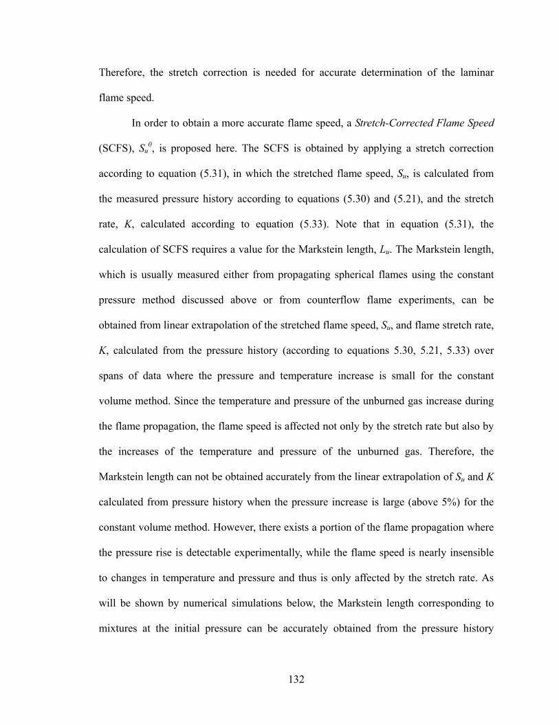
Therefore, the stretch correction is needed for accurate determination of the laminar
flame speed.
In order to obtain a more accurate flame speed, a Stretch-Corrected Flame Speed
(SCFS), Su0, is proposed here. The SCFS is obtained by applying a stretch correction
according to equation (5.31), in which the stretched flame speed, Su, is calculated from
the measured pressure history according to equations (5.30) and (5.21), and the stretch
rate, K, calculated according to equation (5.33). Note that in equation (5.31), the
calculation of SCFS requires a value for the Markstein length, Lu. The Markstein length,
which is usually measured either from propagating spherical flames using the constant
pressure method discussed above or from counterflow flame experiments, can be
obtained from linear extrapolation of the stretched flame speed, Su, and flame stretch rate,
K, calculated from the pressure history (according to equations 5.30, 5.21, 5.33) over
spans of data where the pressure and temperature increase is small for the constant
volume method. Since the temperature and pressure of the unburned gas increase during
the flame propagation, the flame speed is affected not only by the stretch rate but also by
the increases of the temperature and pressure of the unburned gas. Therefore, the
Markstein length can not be obtained accurately from the linear extrapolation of Su and K
calculated from pressure history when the pressure increase is large (above 5%) for the
constant volume method. However, there exists a portion of the flame propagation where
the pressure rise is detectable experimentally, while the flame speed is nearly insensible
to changes in temperature and pressure and thus is only affected by the stretch rate. As
will be shown by numerical simulations below, the Markstein length corresponding to
mixtures at the initial pressure can be accurately obtained from the pressure history
132

during this period and can be utilized in the SCFS method to improve the accuracy of the
flame speed measurement.
For the constant volume method, the pressure history, P=P(t), from the simulation
is used to calculate the flame speed without stretch correction according to equations
(5.30) and (5.21). The SCFS is calculated from the pressure history using the procedure
proposed above. Before obtaining the SCFS, the validity of the theoretical relationships
between the flame radius and pressure given by equation (5.21) and the linear
relationship between the mass fraction of burned gas and pressure rise given by equation
(5.29) is demonstrated by their excellent agreement with numerical simulation of
propagation spherical flames in a closed spherical chamber. The results for a rich H2/air
flame at the equivalence ratio of φ=4 are shown in figure 5.14, which reveals that the
theoretical model agrees well with the direct numerical simulation. Similar results for
other fuels are also obtained, indicating the robustness of the theoretical relationships
given by equations (5.21) and (5.29).
In order to obtain the Stretch-Corrected Flame Speed (SCFS), the Markstein
length, Lu, must be extracted from the pressure history. As mentioned before, the
temperature and pressure of unburned gas increase during flame propagation. As a result,
the Markstein length, Lu, which depends on pressure and temperature, may also change.
In the following, the Markstein length is obtained from two different methods. The first
method (Lu≠const) is to use Rf=Rf(t) results from numerical simulation to calculate the
Markstein length through linear extrapolation of stretched flame speed, Su, and stretch
rate, K, at constant pressure and temperature calculated from the constant pressure
method. This process is repeated to obtain the Markstein length at different temperature
133

and pressures corresponding to those for flames at different sizes in the constant volume
method. Unfortunately, in most experimental measurements of flame speed, it is
impossible to calculate the Markstein length accurately using the above method because a
validated mechanism is usually not available. The second method (Lu= Lu0=const) is to
use the pressure history which is recorded in experiments to obtain the Markstein length
via linear extrapolation of Su and K calculated from pressure history (according to
equations 5.39, 5.21, 5.33). In addition, in order to remove the effect of pressure and
temperature increase, the data range used for the Markstein length calculation is limited
to those with pressure increase lower than 5%. The results show that the Markstein length
obtained by the second method agree well (less than 2% difference) with those obtained
from the first method. The Markstein lengths obtained from the two different methods
proposed above will be utilized to calculate the SCFS.
The propagating spherical flames of different fuels were simulated and the results
are shown in figures 5.15 and 5.16. For a rich H2/air flame of the equivalence ratio of
φ=4, the Markstein length corresponding to mixtures at the initial pressure and
temperature (1 atm, 298 K), is 0.3 mm which is predicted well by both methods. Figure
5.15(a) shows that without the stretch correction the flame speed from the constant
volume method (using equations 5.30 and 5.21) agree well with those from PREMIX
(PREMIX calculations are conducted at different sets of temperature and pressure
according to the expected rise as the flame kernel grows in the constant volume vessel)
only at a very large pressure increase (large Rf/R0). When the pressure increase or the
relative flame radius is small, the discrepancy between the flame speed without and with
stretch correction is more than 20%. This result shows clearly that stretch correction is
134

necessary in the constant volume experiment to obtain a reliable flame speed for small
spherical flames. Figure 5.15 shows that the SCFS agrees very well with those from
PREMIX, even for small pressure increases. Therefore, the accuracy of the measured
flame speed is greatly improved by utilizing the SCFS.
Results indicate that the SCFS using the Markstein lengths from the above two
methods (Lu≠const and Lu=const) agree very well. In fact, using a constant Markstein
length from the second method only slightly over-predicts the stretch effect because the
Markstein length and stretch rate decrease with increasing pressure. As shown in figure
5.15(b), the stretch rate (normalized by the stretch rate at Rf/R0=0.1) quickly decreases
with increasing pressure. This explains why the difference between the SCFS obtained
using the first and second methods is negligible. The success of the second method is
significant for experimental measurements of flame speeds by using the constant volume
method – the SCFS can be obtained directly from the pressure history without any
knowledge of chemical kinetics and transport properties.
For a stoichiometric H2/air flame of φ=1, the unburned Markstein length is 0.03
mm at the initial pressure and temperature of (1 atm, 298 K). Therefore, as expected, the
error caused by neglecting the stretch effect is small (below 5% in this case), which is
also confirmed by results shown in figure 5.16(a). It is seen that for the stoichiometric
H2/air mixture, which has a small unburned Markstein length, the stretch effect is
negligible and the discrepancy between the flame speed without and with stretch
correction is small.
For a lean H2/air flame of φ=0.45, the unburned Markstein length is negative,
Lu=-0.28 mm at the initial pressure and temperature of (1 atm, 298 K). As such, positive
135

flame stretch will increase the flame speed according to equation (5.8). As shown in
figure 5.16(b), flame speed without stretch correction is much larger than the planar
unstretched flame speed predicted by PREMIX. The discrepancy between the flame
speed without and with stretch correction can reach as high as 50% for this case. Figure
5.16(b) shows that after the stretch correction, the flame speed obtained from the constant
volume method agrees well with those computed from PREMIX. Therefore, the above
results show that the accuracy of the flame speed measurement can be greatly improved
by utilizing the SCFS. Of course, in experiments for lean H2/air flames, cellular
instability will greatly affect the flame speed when the flame radius is larger than a
critical value. Nevertheless, the results of lean H2/air flame are presented here in order to
demonstrate the validity of the analytical relation for the stretch effect given by equation
(5.34), and the improvement of the flame speed measurements accuracy by using SCFS.
For a stoichiometric CH4/air flame, similar results to those of the stoichiometric
H2/air shown in figure 5.16(a) are obtained. It is found that the stretch effect is negligible
since the Markstein length is small, which agrees with the prediction from equation
(5.34).
For a lean C3H8/air flame of φ=0.8, the unburned Markstein length is 0.19 mm at
the initial pressure and temperature of (1 atm, 298 K). Figure 5.16(c) shows that when the
pressure increase or the relative flame radius is small, the discrepancy between the flame
speed with and without the stretch correction is more than 20%. After the stretch
correction, the flame speeds from the constant volume method agree very well with those
from PREMIX. Again, the accuracy of the measured flame speed is shown to be greatly
improved by utilizing the SCFS. All the results in figure 5.16 show that the SCFS based
136
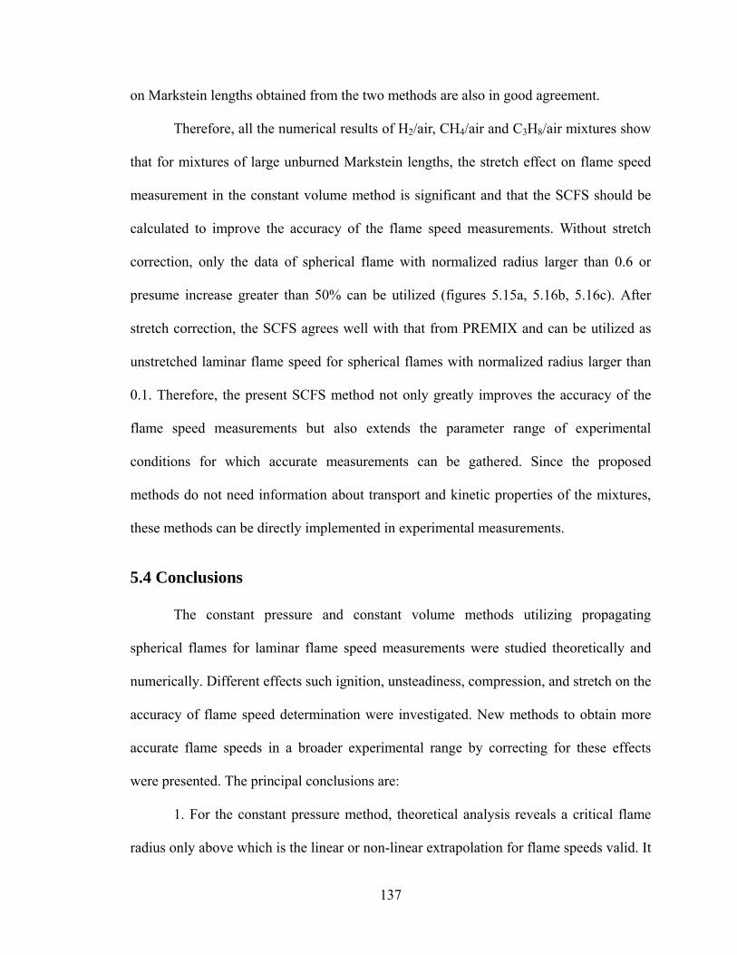
on Markstein lengths obtained from the two methods are also in good agreement.
Therefore, all the numerical results of H2/air, CH4/air and C3H8/air mixtures show
that for mixtures of large unburned Markstein lengths, the stretch effect on flame speed
measurement in the constant volume method is significant and that the SCFS should be
calculated to improve the accuracy of the flame speed measurements. Without stretch
correction, only the data of spherical flame with normalized radius larger than 0.6 or
presume increase greater than 50% can be utilized (figures 5.15a, 5.16b, 5.16c). After
stretch correction, the SCFS agrees well with that from PREMIX and can be utilized as
unstretched laminar flame speed for spherical flames with normalized radius larger than
0.1. Therefore, the present SCFS method not only greatly improves the accuracy of the
flame speed measurements but also extends the parameter range of experimental
conditions for which accurate measurements can be gathered. Since the proposed
methods do not need information about transport and kinetic properties of the mixtures,
these methods can be directly implemented in experimental measurements.
5.4 Conclusions
The constant pressure and constant volume methods utilizing propagating
spherical flames for laminar flame speed measurements were studied theoretically and
numerically. Different effects such ignition, unsteadiness, compression, and stretch on the
accuracy of flame speed determination were investigated. New methods to obtain more
accurate flame speeds in a broader experimental range by correcting for these effects
were presented. The principal conclusions are:
1. For the constant pressure method, theoretical analysis reveals a critical flame
radius only above which is the linear or non-linear extrapolation for flame speeds valid. It
137
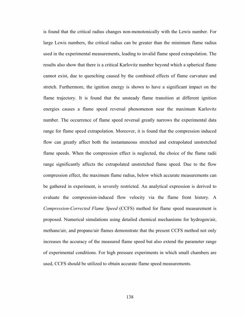
is found that the critical radius changes non-monotonically with the Lewis number. For
large Lewis numbers, the critical radius can be greater than the minimum flame radius
used in the experimental measurements, leading to invalid flame speed extrapolation. The
results also show that there is a critical Karlovitz number beyond which a spherical flame
cannot exist, due to quenching caused by the combined effects of flame curvature and
stretch. Furthermore, the ignition energy is shown to have a significant impact on the
flame trajectory. It is found that the unsteady flame transition at different ignition
energies causes a flame speed reversal phenomenon near the maximum Karlovitz
number. The occurrence of flame speed reversal greatly narrows the experimental data
range for flame speed extrapolation. Moreover, it is found that the compression induced
flow can greatly affect both the instantaneous stretched and extrapolated unstretched
flame speeds. When the compression effect is neglected, the choice of the flame radii
range significantly affects the extrapolated unstretched flame speed. Due to the flow
compression effect, the maximum flame radius, below which accurate measurements can
be gathered in experiment, is severely restricted. An analytical expression is derived to
evaluate the compression-induced flow velocity via the flame front history. A
Compression-Corrected Flame Speed (CCFS) method for flame speed measurement is
proposed. Numerical simulations using detailed chemical mechanisms for hydrogen/air,
methane/air, and propane/air flames demonstrate that the present CCFS method not only
increases the accuracy of the measured flame speed but also extend the parameter range
of experimental conditions. For high pressure experiments in which small chambers are
used, CCFS should be utilized to obtain accurate flame speed measurements.
138

2. For the constant volume method, an analytical expression is derived to evaluate
the stretch effect on the determination of flame speeds. It is found that the stretch effect is
proportional to the Markstein length and inversely proportional to the flame radius. For
mixtures with Lewis numbers greatly deviating from unity, the stretch effect on the flame
speed is significant. A Stretch-Corrected Flame Speed (SCFS) model is then proposed to
obtain accurate flame speed directly from the experimental measurement. The accuracy
of the measured flame speed is greatly improved by using the SCFS method, which is
demonstrated by detailed numerical simulation.
The present results indicate that extrapolation of unstretched flame speeds in
larger bombs at low pressures using typical flame radius ranges yield accurate results
(within 5%) without consideration of compression effects. However, in smaller bombs,
they reveal that the extrapolation is subject to large errors (~15%) if these effects are not
considered. Moreover, the errors become even more serious. The proposed improvements
to the theoretical models not only increases the accuracy of flame speed measurements
but also enable flame speed measurements to be gathered from small bombs, which have
significant advantages in terms of the pressure range, cost, and reduction of flame
wrinkling and radiation effects, without sacrificing accuracy.
Note that the effect of radiative heat loss on the accuracy of flame speed
measurement utilizing propagating spherical flames is not included in the present study.
It has been shown in (Chen et al. 2008c) that radiation has three effects: 1) to decrease the
flame temperature and thus flame speed; 2) to induce inward flow and slow down the
flame propagation; and 3) to preheat the reactants due to absorption. The first effect is
found to be important only for near-limit mixtures having very low laminar flame speed
139

(less than 10 cm/s) and the second effect is found to be important only for highly
radiative mixture (for example, CO2 diluted mixture in oxy-fuel combustion). The third
effect will be discussed in the next chapter. For most mixtures (H2/air, CH4/air, C3H8/air,
etc.) not close to their flammability limits and without CO2 dilution, the effects of
radiation can be neglected.
140
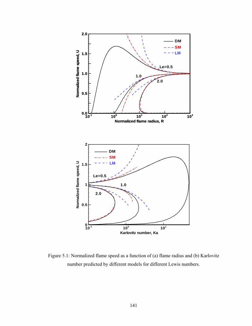
Normalized flame radius, R
Nor
mal
ized
flam
esp
eed,
U
10-1 100 101 102 1030.0
0.5
1.0
1.5
2.0
Normalized flame radius, R
Nor
mal
ized
flam
esp
eed,
U
10-1 100 101 102 1030.0
0.5
1.0
1.5
2.0
1.02.0
Le=0.5
LM
DMSM
Karlovitz number, Ka
Nor
mal
ized
flam
esp
eed,
U
10-1 100 1010
0.5
1
1.5
2
LM
DMSM
Le=0.5
1.0
2.0
Figure 5.1: Normalized flame speed as a function of (a) flame radius and (b) Karlovitz
number predicted by different models for different Lewis numbers.
141
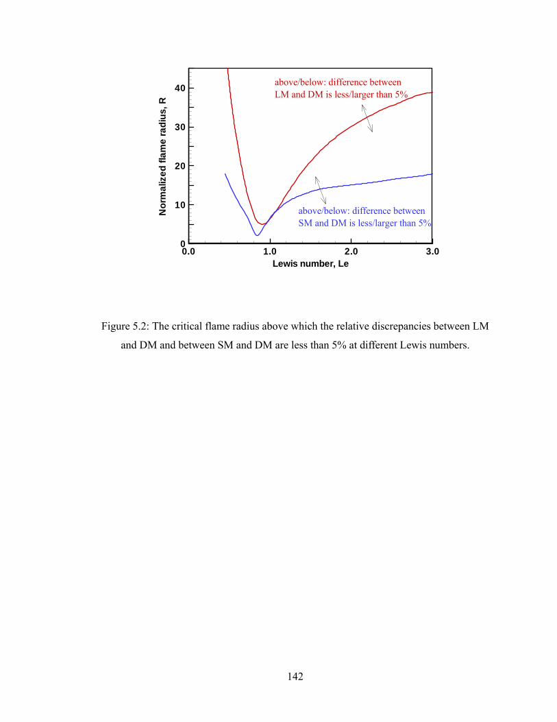
Lewis number, Le
Nor
mal
ized
flam
era
dius
,R
0.0 1.0 2.0 3.00
10
20
30
40 above/below: difference betweenLM and DM is less/larger than 5%
above/below: difference betweenSM and DM is less/larger than 5%
Figure 5.2: The critical flame radius above which the relative discrepancies between LM
and DM and between SM and DM are less than 5% at different Lewis numbers.
142
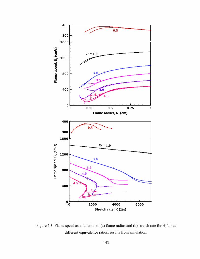
300
4000.5
Flam
esp
eed,
Sb
(cm
/s)
0 0.25 0.5 0.75 10
400
800
1200
1600
ϕ = 1.0
3.5
4.0
4.5
3.0
c
ab
Flame radius, Rf (cm)
300
400
0.5
Flam
esp
eed,
Sb
(cm
/s)
0 2000 4000 60000
400
800
1200
1600
ϕ
3.0
3.5
4.0
4.5
= 1.0
a
cb
Stretch rate, K (1/s)
Figure 5.3: Flame speed as a function of (a) flame radius and (b) stretch rate for H2/air at
different equivalence ratios: results from simulation.
143

Equivalence ratio,
Crit
ical
radi
us,R
c(m
m)
Lew
isnu
mbe
r,Le
0 1 2 3 4 5 60
5
10
15
20
25
-3
-2
-1
0
1
2
ϕ
Figure 5.4: Critical flame radii and Lewis numbers for H2/air at different equivalence
ratios. Data denoted by open triangles are from (Law 2006) and those by squares are from
(Joulin and Mitani 1981).
144
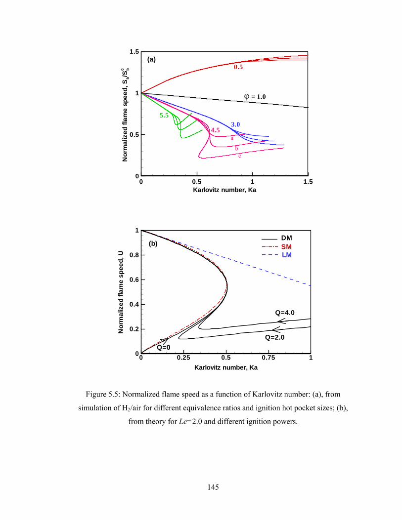
Karlovitz number, Ka
Nor
mal
ized
flam
esp
eed,
Sb/S
b0
0 0.5 1 10
0.5
1
1.5
ϕ = 1.0
.5
3.04.5
5.5
c
a
b
(a)0.5
Karlovitz number, Ka
Nor
mal
ized
flam
esp
eed,
U
0 0.25 0.5 0.75 10
0.2
0.4
0.6
0.8
1
LMSMDM
Q=0Q=2.0
Q=4.0
(b)
Figure 5.5: Normalized flame speed as a function of Karlovitz number: (a), from
simulation of H2/air for different equivalence ratios and ignition hot pocket sizes; (b),
from theory for Le=2.0 and different ignition powers.
145

Flame radius, Rf (mm)
Dis
tanc
ebe
twee
nT=
400K
and
1000
K,d
(mm
)
0 2 4 6 80.2
0.3
0.4
0.5
0.6
0.7
0.8
c
b
a
10
Figure 5.6: Variation of flame thickness during flame propagation from different
initiation kernels for H2/air (φ=4.5).
Karlovitz number, Ka
Nor
mal
ized
flam
esp
eed,
Sb/S
b0
0 0.25 0.5 0.750.0
0.2
0.4
0.6
0.8
1.0
2 atm
1 atm4 atm
Figure 5.7: Normalized flame speed as a function of Karlovitz number for H2/air (φ=5.0)
at different pressures and ignition hot pocket size.
146
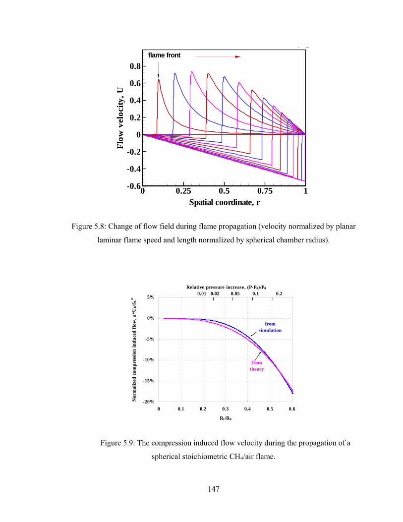
Spatial coordinate, r
Flow
velo
city
,U
0 0.25 0.5 0.75 1-0.6
-0.4
-0.2
0
0.2
0.4
0.6
0.8flame front
r 1
Figure 5.8: Change of flow field during flame propagation (velocity normalized by planar
laminar flame speed and length normalized by spherical chamber radius).
-20%
-15%
-10%
-5%
0%
5%
0 0.1 0.2 0.3 0.4 0.5 0.6
Rf/R0
Nor
mal
ized
com
pres
sion
indu
ced
flow
, a*U
b/SL
0
0.01 0.02 0.05 0.1 0.2Relative pressure increase, (P-P0)/P0
fromtheory
fromsimulation
Figure 5.9: The compression induced flow velocity during the propagation of a
spherical stoichiometric CH4/air flame.
147

0.4
0.6
0.8
1
1.2
0 0.1 0.2 0.3 0.4Normalized stretch rate, K'
Nor
mal
ized
flam
e sp
eed,
Su/
S L0
0.5 0.4 0.3 0.2 0.1
Normalized flame radius, Rf/R0
Su=a*(dRf/dt-Ub)Su=a*dRf/dt
Su=a(Tu)*(dRf/dt-Ub)
Figure 5.10: Normalized stretched flame speed as a function of normalized stretch rate
and flame radius for a stoichiometric CH4/air flame.
-30%
-20%
-10%
0%
10%
to Rf/R0
Su0 /S
L0 -1
from from from
0.2 0.3 0.4 0.5
using "Su=a*dRf/dt"uncorrected flame speed
compression corrected flame speed using "Su=a*(dRf/dt-Ub)"
Rf/R0=0.1
Rf/R0=0.2Rf/R0=0.3
Figure 5.11: Accuracy of the unstretched flame speed with and without compression
correction using different flame radius ranges for a stoichiometric CH4/air flame.
148

-20%
-15%
-10%
-5%
0%
5%
to Rf/R0
Su0 /S
L0 -1
from =0.1from =0.2from =0.3
0.2 0.3 0.4 0.5
using "Su=a*dRf/dt"uncorrected flame speed
compression corrected flame speedusing "Su=a*(dRf/dt-Ub)"
Rf/R0
Rf/R0
Rf/R0
-30%
-20%
-10%
0%
to Rf/R0
Su0 /S
L0 -1
from from from
0.2 0.3 0.4 0.5
using "Su=a*dRf/dt"uncorrected flame speed
compression corrected flame speedusing "Su=a*(dRf/dt-Ub)"
Rf/R0=0.1
Rf/R0=0.2
Rf/R0=0.3
(b)
Figure 5.12: Accuracy of the unstretched flame speed with and without compression
correction using different flame radius ranges for (a), a stoichiometric H2/air flame; (b), a
stoichiometric C3H8/air flame.
149

0%
5%
10%
15%
20%
25%
30%
0.2 0.3 0.4 0.5 0.6 0.7 0.8 0.9 1Normalized flame radius, Rf/R0
Stre
tch
effe
ct o
n fla
me
spee
d, 1
-/S
u0
1.01 1.02 1.05 1.1 1.2 1.5 2 3 4 5 8Normalized pressure, P/P0
Stre
tch
effe
ct o
n fla
me
spee
d, 1
-Su/
S u0
Figure 5.13: The stretch effect on the flame speed according to equation (5.34) with
Pe/P0=8.27, γ=1.4, Lu=0.25 mm, R0=6 cm.
150
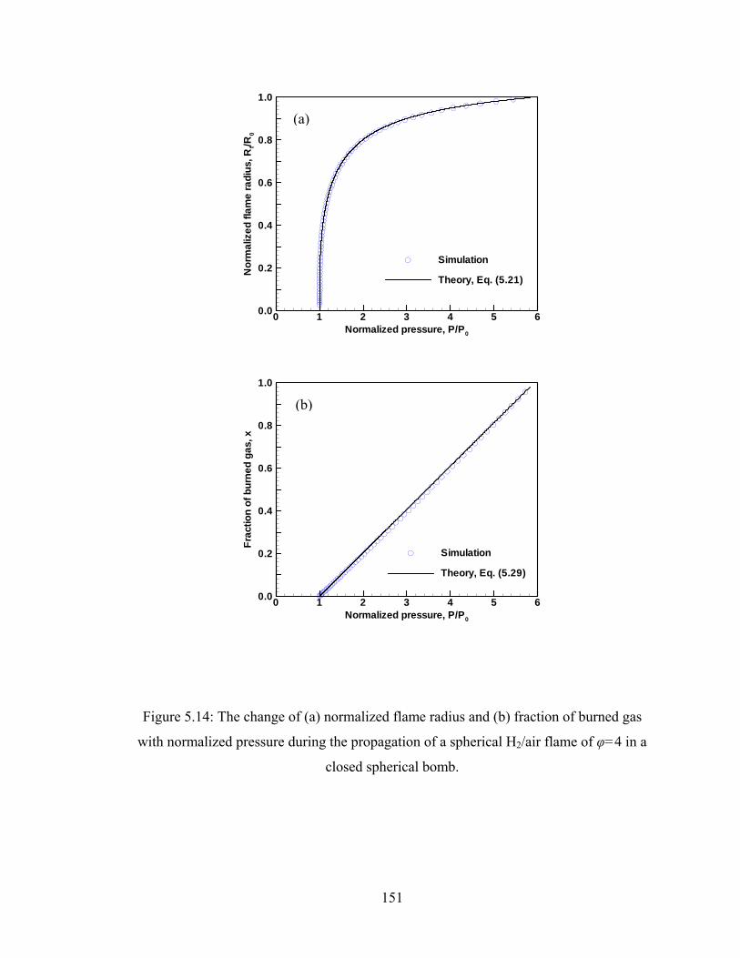
Normalized pressure, P/P0
Nor
mal
ized
flam
era
dius
,Rf/R
0
0 1 2 3 4 50.0
0.2
0.4
0.6
0.8
1.0
Simulation
Theory, Eq. (5.21)
(a)
6
Normalized pressure, P/P0
Frac
tion
ofbu
rned
gas,
x
0 1 2 3 4 50.0
0.2
0.4
0.6
0.8
1.0
Simulation
Theory, Eq. (5.29)
(b)
6
Figure 5.14: The change of (a) normalized flame radius and (b) fraction of burned gas
with normalized pressure during the propagation of a spherical H2/air flame of φ=4 in a
closed spherical bomb.
151

Normalized flame radius, Rf/R0
Flam
esp
eed
norm
aliz
edby
SL0
0 0.2 0.4 0.6 0.8 10.5
1
1.5
2
Normalized pressure, P/P0
54321.51.21.11.051.0 1.02
PREMIX
SCFS, Su0 (Lu=const)
without stretch correction (Su)SCFS, Su
0 (Lu=const)
1.01
(a)
Normalized flame radius, Rf/R0
Nor
mal
ized
stre
tch
rate
,K/K
'
0 0.2 0.4 0.6 0.8 10
0.2
0.4
0.6
0.8
1
Normalized pressure, P/P0
54321.51.21.11.051.011.02
(b)
0
54321.51.21.11.051.0 1.021.01
Figure 5.15: (a) Flame speed with and without stretch correction and (b) normalized
stretch rate as a function of normalized flame radius and pressure for a H2/air flame of
φ=4.
152

Normalized flame radius, Rf/R0
Flam
esp
eed
norm
aliz
edby
SL0
0 0.2 0.4 0.6 0.8 10.5
1
1.5
2
2.5
Normalized pressure, P/P0
84321.51.21.11.051.0 1.02
PREMIX
SCFS, Su0 (Lu=const)
without stretch correction (Su)SCFS, Su
0 (Lu=const)
51.01
Normalized flame radius, Rf/R0
Flam
esp
eed
norm
aliz
edby
SL0
0 0.2 0.4 0.6 0.8 10.5
1
1.5
2
Normalized pressure, P/P0
54321.51.21.11.051.0 1.02
PREMIX
SCFS, Su0 (Lu=const)
without stretch correction (Su)SCFS, Su
0 (Lu=const)
1.01
(a)
(b)
153

Normalized flame radius, Rf/R0
Flam
esp
eed
norm
aliz
edby
SL0
0 0.2 0.4 0.6 0.8 10.6
0.8
1
1.2
1.4
Normalized pressure, P/P0
84321.51.21.11.051.0 1.02
PREMIX
SCFS, Su0 (Lu=const)
without stretch correction (Su)SCFS, Su
0 (Lu=const)
51.01
(c)
Figure 5.16: Flame speed with and without stretch correction as a function of normalized
flame radius and pressure for (a), a H2/air flame of φ=1; (b), a H2/air flame of φ=0.45;
(c), a C3H8/air flame of φ=0.8.
154

Chapter 6: Effect of Radiation on Flame Propagation
and Extinction
In this chapter, the effect of radiation on flame propagation and extinction is
investigated. In the first part, the effect of radiative heat loss on both outwardly and
inwardly propagating spherical flames is studied using asymptotic analysis for a
simplified quasi-planar thermo-diffusion flame structure. In the second part, the effects of
spectral-dependent radiation and absorption on the flammability limits and flame speed
are investigated experimentally and numerically for CO2 diluted outwardly propagating
CH4/O2/He flames at normal and elevated pressures. In the third part, the combined
effects of radiation, curvature, and stretch on the extinction of premixed counterflow and
tubular flames are analyzed.
6.1 Radiation Effect on Propagating Spherical Flames
6.1.1 Introduction
Radiation heat transfer is well known to be a dominant mechanism for near-limit
flames. Extensive studies have been conducted to investigate the effects of radiation,
stretch, and curvature on flame extinction by using the counterflow flames, outwardly
propagating spherical flames (OPF), and tubular flames, all of which have positive flame
stretch rate. To study the effect of negative flame stretch rate, the inwardly propagating
spherical flames (IPF) can be utilized. The quenching of IPF has been studied
theoretically and numerically in (Frankel and Sivashinsky 1984; Flaherty et al. 1985; Sun
and Law 1998). The quenching was found to take place at non-zero velocity of the flame
front for mixtures with Lewis number less than unity due to the negative stretch rate of
155

IPF. For mixtures with Lewis number larger than unity, it was shown that extinction also
occurs for IPF due to depletion of the upstream mixture (Sun and Law 1998). Both the
OPF and IPF were studied in (Sun et al. 1999) to show the linear relationship between
stretched flame speed and flame stretch rate. However, radiative heat loss was not
considered in all of the above studies on IPF. As a result, how radiation affects the
propagation and extinction of IPF is not well understood. Furthermore, as discussed in
the previous chapter, the method utilizing propagating spherical flames in a closed
chamber is currently one of the most favourable methods for measuring laminar flame
speeds and Markstein lengths. Radiation transfer is inevitable in practical experiments
and the effect of radiation on flame speed measurements has been investigated in
previous studies (Taylor 1991; Chen et al. 2007a; Chen et al. 2008c). However, there is
no study about radiation effect on the Markstein length. Therefore, how the Markstein
length is affected by radiation remains unclear.
The objective of this study is to answer the above two questions. Both the OPF
and IPF with radiative loss will be investigated and the emphasis is on studying the
effects of radiative loss and preferential diffusion on the flame propagation speed,
Markstein number, and flame extinction.
6.1.2 Mathematical Model and Asymptotic Solutions
Figure 6.1 shows the schematic diagrams of the OPF and IPF investigated in the
present study. The mathematical model for the OPF and IPF is similar to that presented in
Chapter 2. Unlike Chapter 2 where emphasis is on the initiation of OPF, here we focus on
the propagation and extinction of OPF and IPF. The large flame radius assumption used
in (Frankel and Sivashinsky 1983; Frankel and Sivashinsky 1984) is employed here,
156

under which the nondimensional governing equations, (2.9a, 2.9b), can be simplified as
ωξξ
+⋅−=+− Thd
TdddT
RU 2
2
)2( (6.1)
ωξξ
⋅−=+− Led
YdddY
RLeU 2
2
)2( (6.2)
where )(tRr −=ξ is the moving coordinate attached to the propagating flame front,
R=R(t), in which the thermo-diffusion structure of the flame is quasi-planar, i.e. R>>ξ
(Frankel and Sivashinsky 1983).
Following the same asymptotic analysis procedure presented in Chapter 2, the
following algebraic system of equations for normalized flame propagation speed, U
(U=│dR/dt│=│V-2/R│), normalized flame radius, R, and normalized flame temperature,
Tf, are obtained (the normalization is presented in Chapter 2)
))1(
12
exp()11(242
f
ff T
TZLeR
VhVTσσ −+
−=⎥⎦
⎤⎢⎣⎡ −+±=+ (6.3)
where ‘+’ is for OPF and ‘–’ for IPF. Eliminating the flame temperature and setting
L=2Zh, where h~O(1/Z) and L~O(1), we have
LRdt
dRLeR
ZRdt
dRRdt
dR−+−−=++ )2)(11(2)2(])2ln[()2( 22 (6.4)
Using the above relationship, the effect of radiative loss on OPF and IPF could be
investigated by comparing the normalized flame propagation speed, U=│dR/dt│, at
different flame radii, R, and radiative loss intensities, L. The preferential diffusion effect
can also be studied by changing the Lewis number in equation (6.4). The general theory
presented in Chapter 2, equation (2.14), which works for OPF for all flame radii range, is
found to reduce to the present result, equation (6.4), in the limit of R>>1 for OPF. Figure
157

6.2 shows the flame propagation speed as a function of flame radius for OPF predicted by
the present simplified model, equation (6.4), and the detailed model, equation (2.14). It is
seen that the prediction from the simplified model agrees well with that from the detailed
model at different Lewis numbers and radiative losses. It is noted that the detailed model
only works for OPF and there is no counterpart theory for IPF; while the simplified
model under the assumption of large flame radius works for both OPF and IPF.
The present simplified model recovers previous results in different limiting cases.
Without radiative loss, L=0, equation (6.4) reduces to that of adiabatic propagating
spherical flames studied in (Frankel and Sivashinsky 1983). Moreover, by changing the
curvature from 2/R to 1/R in equation (6.4), the same result for nonadiabatic propagating
cylindrical flames as that presented in (Mitani 1980) is obtained. In the limit of ∞→R ,
equation (6.4) recovers the classical theory of flammability limit for planar flames (Joulin
and Clavin 1979)
LUU −=])ln[()( 2020 (6.5)
where U0 is utilized to denote the nondimensional (normalized by adiabatic planar flame
speed) plane flame speed with radiative loss. According to equation (6.5), the
flammability limit for planar flame is eL /1* = and . 2/10* −= eU
For both OPF and IPF, the Karlovitz number is defined as K=(2/R)(dR/dt)
(Clavin 1985; Law 2006). When it is small, │K│<<1, there is a linear relationship
between U and K (Clavin 1985)
KMaUU ⋅−≈ 0 (6.6)
158
where Ma is the Markstein number. Using Taylor expansion for equation (6.4) at small K,
the linear relationship, equation (6.6), as well as the following expression for the
Markstein number is obtained
]1)ln(2)[()1)(12/(1
00
1
0 +−−
−=−
UULeZ
UMa (6.7)
According to equations (6.5) and (6.7), it is seen that the Markstein number is
affected not only by the Lewis number but also by the radiative loss. For adiabatic case
(L=0, U0=1), the adiabatic Markstein length is (the subscript 0 means at zero radiative
loss, i.e. adiabatic; while the superscript 0 means at zero stretch rate, i.e. unstretched)
)1)(2/( 110 −−= −− LeZLeMa (6.8)
which is the same as that derived for adiabatic counterflow premixed flames (Law 2006).
In (Law 2006) , the following relationship is proposed for stretched premixed flames with
small radiative losses (L<<1)
2)]11(
21[1 LK
LeZ
LeU −−−−≈ (6.9)
according to which the Markstein length is not affected by radiative loss and is a constant
given by equation (6.8). This is not contradictory with the present result. The relationship
given by equation (6.9) works only for small radiative loss, while the results given by
equations (6.6) and (6.7) work well not only for small radiative loss but also for large
radiative loss. As a result, the present theory works for a broader range of radiative loss
and thus the radiation effect on flame propagation speed as well as Markstein length at
different Lewis numbers can be investigated using equation (6.4).
159

6.1.3 Results and Discussions
Figure 6.3 shows the normalized flame propagation speed as a function of flame
radius for OPF and IPF with different radiative loss intensities, L, and Lewis numbers,
Le. The same Zel’dovich number, Z=10, as used in Chapter 2 is used here. The results for
OPF are consistent with those shown in figures 2.3(a), 2.4(a), and 2.5(a). At a given
Lewis number and radiative loss, there are two solutions of flame propagation speed for
one specific flame radius: the fast stable one and the slow unstable one (only the fast
branch is shown for Le=1.0). Extinction occurs at the turning point where the fast branch
meets the slow branch (there is no extinction for Le=1.0). Figure 6.3 clearly shows that
the U-R relation and flame extinction is strongly affected by the Lewis number and
radiative loss. For the same Lewis number, the U-R diagram of OPF shows totally
opposite trends compared with that of IPF. This is because the OPF has positive stretch
rate, K=(2/R)(dR/dt)>0, while the IPF has negative stretch rate, K=(2/R)(dR/dt)<0. For a
Lewis number less (larger) than some critical Lewis number, Le* (which is less than 1.0),
the positive stretch rate of OPF strengths (weakens) the flame while the negative stretch
rate of IPF weakens (strengths) the flame (Law 2006). As a result, for Le=0.5, the flame
propagation speed (the fast stable branch) of both OPF and IPF decreases monotonically
during the propagation; while for Le=1.0 and Le=2.0, it monotonically increases during
the propagation (note that the magnitude of stretch rate change inversely with flame
radius).
To investigate the effects of radiation and flame stretch on spherical flame
propagation and extinction, the normalized flame propagation speed as a function of
stretch rate is shown in figure 6.4. As shown in figures 6.3 and 6.4, for Le=0.5, the flame
160
extinction occurs for IPF even when the radiative heat loss is smaller than the one
corresponding to the planar flame flammability limit, eL /1* = ; while OPF (which is
called self-extinguish flame, SEF) still exits even for mixtures below the flammability
limit, . For OPF, the existence of SEF for small Lewis numbers is
because the flame stretch enhancement is greater than radiative loss when the flame
radius is small (Ronney 1985; Ronney 1988). For IPF, extinction is caused by the
continuously decreasing flame stretch rate (it is negative and its absolute value increasing
during flame propagation) which weakens the flame during flame propagation before the
extinction point is reached. The opposite trend is shown for Le=2.0. Similar results from
simulations of adiabatic IPF at different Lewis numbers were found in (Flaherty et al.
1985; Sun and Law 1998), which confirms the validity of the present theoretical
prediction. Furthermore, figures
*/14.0 LeL =>=
6.3 and 6.4 also show that the radiative loss strongly
affects both OPF and IPF and flame extinction occurs earlier at higher radiative loss.
Therefore, at the same radiative loss, for mixture with small Lewis number
(Le<Le*), the OPF/IPF propagates faster/slower than the planar propagating flame and
the flammability limit is extended/narrowed due to the positive/negative flame stretch;
while for mixture with large Lewis number (Le>Le*), the opposite trend happens. The
change of flammability limit caused by stretch rate coupled with preferential diffusion
effect (Lewis number effect) is further shown in figures 6.5. The turning point on the
solid curve, which is the solution as R→∞, corresponds to the flammability limit for the
planar flame, and only the upper fast branch is stable and thus physically realistic. The
dashed and dash-dotted lines represent solutions for flames at finite radii (thus finite
stretch rate). The flammability region is either extended or reduced, depending on the
161

value of the Lewis number and the sign of stretch rate: for mixture with small Lewis
number (Le<Le*), it is extended for positive stretch (OPF) and reduced for negative
stretch (IPF); while for mixture with large Lewis number (Le>Le*), it is extended for
negative stretch (IPF) and reduced for positive stretch (OPF). The present results on
stretch rate and Lewis number effects for OPF and IPF are consistent with those for OPF
in (Bechtold et al. 2005) and counterflow flames presented in (Law 2006).
Figure 6.4 shows that the Markstein length (which is equal to -1.0 multiplying the
gradient in the U-K plot at K close to zero) is strongly affected by radiative loss. The
Markstein length can be evaluated based on equation (6.7). Figure 6.6 shows the
Markstein number for different Lewis numbers and radiative loss. It is seen that for small
radiative loss, the Markstein length is close to that of the adiabatic flame, Ma0. However,
when the radiative loss is large, the Markstein length is strongly affected by radiative
loss, especially when L is close to the value corresponding to the flammability limit, L*.
Moreover, the change of the Markstein length due to radiative loss also strongly depends
on the Lewis number.
Figure 6.7 shows the normalized Markstein number as a function of Lewis
number for different radiative loss. It is found that the normalized Markstein number
varies non-monotonically with the Lewis number and it reaches infinity at Le=0.8 due to
the appearance of zero Ma0 for Z=10 (according to equation (6.8), Ma0 is zero at
Le=1-2/Z). With increasing radiative loss, the magnitude of the Markstein number always
increases for Le<0.8. For 0.8<Le<1.0, the magnitude of the Markstein length can be
smaller than the adiabatic Markstein length. For Le>1.0, the normalized Markstein
number is always greater than unity and increases with radiative loss.
162
6.1.4 Summary
The OPF and IPF at large flame radii were studied using asymptotic analysis. A
general correlation between flame propagation speed and flame radius for both OPF and
IPF was derived and utilized to study the effects of radiative loss and preferential
diffusion on the flame propagation speed, Markstein number, and flame extinction. The
following conclusions are made:
1. The flame propagation speed, Markstein number, and flame extinction are
strongly affected by the Lewis number as well as the radiative loss. Opposite trends for
the change of flame propagation speed during flame propagation are shown for OPF and
IPF for different Lewis numbers. The positive/negative stretch rate of OPF/IPF is shown
to enhance/weaken the flame at small Lewis numbers and to weaken/enhance the flame at
large Lewis numbers.
2. The flammability region is found to be extended for positive stretch (OPF) and
reduced for negative stretch (IPF) for mixtures with small Lewis numbers; and it is
extended for negative stretch (IPF) and reduced for positive stretch (OPF) for mixtures
with large Lewis number.
3. A correlation for the Markstein length at different Lewis numbers and radiative
loss was presented. The Markstein length is strongly affected by radiative loss and Lewis
number.
163

6.2 Radiation Reabsorption Effect on Flame Speed and Flammability
Limits
6.2.1 Introduction
In the previous section, radiative loss is simplified as a linear function of
temperature in theoretical analysis. However, in practical problems, thermal radiation not
only changes nonlinearly with temperature but also strongly depends on the mixture
composition and pressure. Furthermore, radiation has a strong spectral dependence and
can act not only as a heat sink due to emission but also as a heat source due to absorption.
In this part, the CO2 diluted outwardly propagating CH4/O2/He flames will be used to
study the effects of the spectral dependent radiation and absorption on flame speed and
flammability limit.
6.2.2 Experimental and Numerical Specifications
The experimental measurements of flame speed were conducted in a
dual-chambered, pressure-release type high pressure combustion facility at normal
gravity (Qin and Ju 2005). This type of dual chamber design was first reported by Tse et
al. (Tse et al. 2000). Due to the effect of buoyancy, the maximum test pressure was
limited to 5 atm. The combustible mixture was spark-ignited at the center of the inner
chamber with minimum ignition energy so as to minimize ignition disturbances. The
flame propagation sequence was imaged with Schlieren photography and a high-speed
digital video camera (Photron Fastcam APX) with 4 μs shutter speed and a framing rate
of 8000 fps. 1024 pixels were used for 5 cm width domain in the horizontal direction.
Data reduction was performed only for flame radii between 1.0 and 2.5 cm. Pressure
increase is negligible since the volume of the chamber is approximately 100 times larger
164
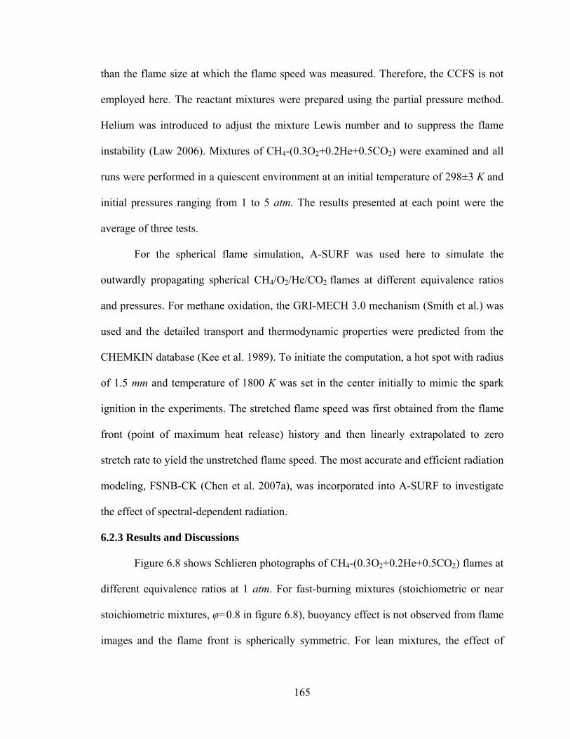
than the flame size at which the flame speed was measured. Therefore, the CCFS is not
employed here. The reactant mixtures were prepared using the partial pressure method.
Helium was introduced to adjust the mixture Lewis number and to suppress the flame
instability (Law 2006). Mixtures of CH4-(0.3O2+0.2He+0.5CO2) were examined and all
runs were performed in a quiescent environment at an initial temperature of 298±3 K and
initial pressures ranging from 1 to 5 atm. The results presented at each point were the
average of three tests.
For the spherical flame simulation, A-SURF was used here to simulate the
outwardly propagating spherical CH4/O2/He/CO2 flames at different equivalence ratios
and pressures. For methane oxidation, the GRI-MECH 3.0 mechanism (Smith et al.) was
used and the detailed transport and thermodynamic properties were predicted from the
CHEMKIN database (Kee et al. 1989). To initiate the computation, a hot spot with radius
of 1.5 mm and temperature of 1800 K was set in the center initially to mimic the spark
ignition in the experiments. The stretched flame speed was first obtained from the flame
front (point of maximum heat release) history and then linearly extrapolated to zero
stretch rate to yield the unstretched flame speed. The most accurate and efficient radiation
modeling, FSNB-CK (Chen et al. 2007a), was incorporated into A-SURF to investigate
the effect of spectral-dependent radiation.
6.2.3 Results and Discussions
Figure 6.8 shows Schlieren photographs of CH4-(0.3O2+0.2He+0.5CO2) flames at
different equivalence ratios at 1 atm. For fast-burning mixtures (stoichiometric or near
stoichiometric mixtures, φ=0.8 in figure 6.8), buoyancy effect is not observed from flame
images and the flame front is spherically symmetric. For lean mixtures, the effect of
165

buoyancy is noticeable and the flame front reaches the top edge of the photograph before
reaching the bottom. Here, we define the 1-g downward flammability limit, Φd, as in the
limiting mixture in which the flame can propagate throughout the entire chamber. For the
present CH4-(0.3O2+0.2He+0.5CO2) mixture, the downward flammability limit is
Φd=0.50. Below this limit, e.g. for leaner mixtures (φ=0.49 in figure 6.8), the flame
cannot propagate downward against buoyancy forces. After reaching the top of the inner
chamber, the flame spreads out and propagates downward. Although the mixture at this
condition is still flammable, the flame front location is hard to determine and flame speed
data are not extracted for these cases. At elevated pressures, buoyancy effect is enhanced
with the increase of mixture density. For example, at 5 atm the downward flammability
limit becomes Φd=0.57.
Figure 6.9 shows the measured and predicted flame speeds of
CH4-(0.3O2+0.2He+0.5CO2) flames at different equivalence ratios at 1 atm. For
comparisons, three radiation models were employed. First is the optically thin model
(OPTM) (Ju et al. 1997) in which no radiation absorption is considered. The second is the
SNB gray band model in 1D planar geometry (SNB-GB1D) (Kim et al. 1991; Liu et al.
1998) in which gray gas model is used at each band (375 bands in total) and radiation
absorption is solved in the one-dimensional slab rather than in spherical geometry. The
third one is the FSNB-CK model (Chen et al. 2007a) in which spectral radiation is solved
in the spherical coordinate. Furthermore, the volumetric radiative loss and temperature
distributions predicted from OPTM, SNB-GB1D and FSNB-CK for a flame at
equivalence ratio of 0.6 and flame radius of 2.4 cm are plotted in figure 6.10.
Figure 6.9 shows that the optically thin model under-predicts the flame speed.
166

This is because OPTM model over-predicts the radiative heat loss and the flame
temperature decreases significantly in the burned zone (figure 6.10). However, for the
FSNB-CK model, it is seen that because of radiation absorption, the radiative loss in the
burned zone becomes much smaller. A significant amount of radiative loss from the
burned zone is reabsorbed by the unburned mixture (see the part with negative heat loss
in figure 6.10). This means that the radiation absorption in CO2-diluted flames increases
the flame speed by reducing the net heat loss and that the optically thin model is not
applicable. As the equivalence ratio decreases, figure 6.9 shows that radiation absorption
plays an important role in increasing the flame speed and extending the flammability
limit. On the other hand, the SNB gray band model in 1D geometry over-predicts the
flame speed. This over-prediction comes from two sources. One is that the employment
of one-dimensional radiation geometry in which less radiation emission in the burned gas
than that in the spherical flame was calculated (compare the radiation predicted by
FSNB-CK(planar) and FSNB-CK(spherical) in figure 6.10); and the second is that the
gray narrow band assumption increases the radiation absorption (compare the radiation
predicted by FSNB-CK(planar) and SNB-GB1D in figure 6.10). The present FSNB-CK
model greatly improves the accuracy of the flame speed prediction. A slight
over-prediction may result from the linear extrapolation method for flame speed because,
strictly speaking, the radiation enhancement does not linearly increase with the flame
radius. This improvement is because the radiation in spherical flame geometry is
appropriately solved and the spectral radiation in each band is accurately treated by using
the cumulative function of k-distribution from the direct Laplace transform instead of the
simple gray gas assumption.
167

Theoretical analysis in (Joulin and Deshaies 1986) shows that radiation
absorption has less effect as pressure increases because the total chemical heat release
increases with the pressure. In order to examine the effect of pressure, the radiation
absorption effect and comparison of different radiation models for
CH4+(0.3O2+0.2He+0.5CO2) mixtures at 2 atm and 5 atm is shown in figure 6.11. It is
seen that radiation absorption becomes much stronger than that at 1 atm. Different from
the theory (Joulin and Deshaies 1986), the present result shows that radiation absorption
increases with pressure. This is because an infinite optical thickness was assumed in the
theory (Joulin and Deshaies 1986) so that all the radiative loss from the burned zone is
absorbed by the unburned mixture. In the present experiment, the optical thickness is
finite (about 1.0~6.0 estimated from OPTM) so that the increase of pressure enlarges the
optical thickness and radiation absorption. Again, for the same reason, it is clearly seen
that the present FSNB-CK model predicts the flame speed much better than SNB-GB1D.
With a further increase of pressure to 5 atm, figure 6.11 shows that the radiation
absorption effect further increases.
To further demonstrate the pressure effect on radiation absorption, the normalized
flame speed increase due to radiation absorption at different equivalence ratios is plotted
in figure 6.12. It is seen that radiation absorption enhancement on the flame speed is
linearly dependent on pressure. This linear dependence is caused by the increase of the
optical thickness. In addition, figure 6.12 shows that with decreasing equivalence ratio,
the effect of radiation absorption on flame speed becomes more significant. Therefore, it
can be concluded that although the pressure increase leads to an increased chemical heat
release, the effect of radiation absorption on flame speed enhancement still increases and
168

it becomes increasingly important for lean flames.
As discussed above, radiation absorption depends on the optical thickness.
Therefore, it is of interest to show how radiation absorption enhancement on the flame
speed depends on the flame size so that a flamelet model can be used to correct the
radiation absorption effect in turbulence modeling. According to the theory in (Joulin and
Deshaies 1986), the flame speed is related to the Boltzmann number, B, by
( ) BSSSS LLLL =00 /ln)/( , ()2/()( 200
40
4adPLad TCSRTTEB ρσ −= 6.10)
where E, R, σ, and CP denote the activation energy, universal gas constant,
Stefan-Boltzmann constant, and the specific heat, respectively. Tad is the adiabatic flame
temperature, and ρ0 and T0 are the unburned gas density and temperature. Therefore, B
represents the radiation absorption effect on the increase of flame speeds. The effective B
numbers estimated from theory (Joulin and Deshaies 1986) and computation (by using SL
from simulation and the first equation of equation (6.10)) as a function of flame size are
plotted in figure 6.13. Note that in calculating the B number, the flame stretch effect is
already excluded by comparing the radiative flames with the adiabatic flames. It is seen
that the radiation absorption effect predicted by the theory is two orders of magnitude
higher than that predicted by the FSNB-CK model. In addition, the theory predicts a
constant B number with increasing flame radius. This is also because of the assumption
of large optical thickness. The FSNB-CK model predicts a negative B number at small
flame radius and an increasing dependence of B on the flame radius. This means that at
small flame radius, although radiation absorption can enhance the flame speed, the final
flame speed remains below the adiabatic flame speed. However, with increasing flame
radius, the optical thickness increases, yielding an increase in the B number. Again, for
169
the optically thin model, the predicted B number is much lower. At high pressures,
similar trends are also found except that the B number becomes positive at 2 atm.
Therefore, by computing the B number for a given optical thickness, the radiation
absorption effect could be employed in flamelet models for turbulent modeling.
6.2.4 Summary
The spectral-dependent radiation absorption effect on flame speed enhancement
was measured by using CO2-diluted CH4–O2 mixtures at normal and elevated pressures.
The following conclusions are drawn from this study:
1. Radiation absorption increases the flame speed and extends the flammability
limit. This enhancement effect also increases with pressure. The spectral-dependent
radiation absorption needs to be included in any quantitative predictions of flame speed
and flammability limit with CO2 addition.
2. The FSNB-CK radiation model can well reproduce the measured flame speed.
The SNB narrow-band gray model over-predicts the flame speed while the optically thin
model significantly under-predicts the flame speed.
3. The radiation absorption effect increases with flame size and pressure. The
theory based on gray gas model over-predicts the radiation absorption by two-orders. The
effective Boltzmann number is extracted from the present radiation modeling and can be
applied to flamelet modeling in turbulent flow.
4. Flame geometry has a significant effect on flame radiation. In spherical flame
modeling, the one-dimensional slab radiation model over-predicts the radiation
absorption.
170
6.3 Radiation Effect on Premixed Counterflow and Tubular Flames
6.3.1 Introduction
It is well known that curved flame fronts prevail in turbulent combustion and the
effect of curvature on flame propagation is important, especially for near-limit flames.
Therefore, in order to extend the flammability and to improve flame stability, it is
particularly important to understand how the coupling of thermal radiation, flame
curvature, and stretch affects the flame speed and extinction limits. In the previous two
sections, the effect of radiation is studied for propagating spherical flames, in which the
flame stretch and flame curvature both change and it is difficult to investigate the pure
curvature effect. In this part, the steady tubular and counterflow flames are investigated
and by comparing the flame dynamics of these two flames at the same stretch rate and
radiation intensity, the curvature effect on the near-limit radiative flames are
demonstrated.
6.3.2 Mathematical Model and Asymptotic Solutions
In order to study the effect of flame curvature, two kinds of flame configurations
are considered in this study. The first one is the premixed tubular flame shown in figure
6.14(a). Combustible mixture is injected toward the concentric inner tube (stagnation
surface) from the inner wall of the porous outer tube. A positively stretched tubular flame
with well-defined flame curvature can be stabilized between the inner and outer tubes
(Takeno et al. 1986; Mosbacher et al. 2003; Wang et al. 2006). The inner tube is
introduced here to change the flame curvature (Mosbacher et al. 2003; Wang et al. 2006;
Yokomori et al. 2006). The second configuration is the premixed planar counterflow
flame shown in figure 6.14(b). This flame is also positively stretched but has no flame
171
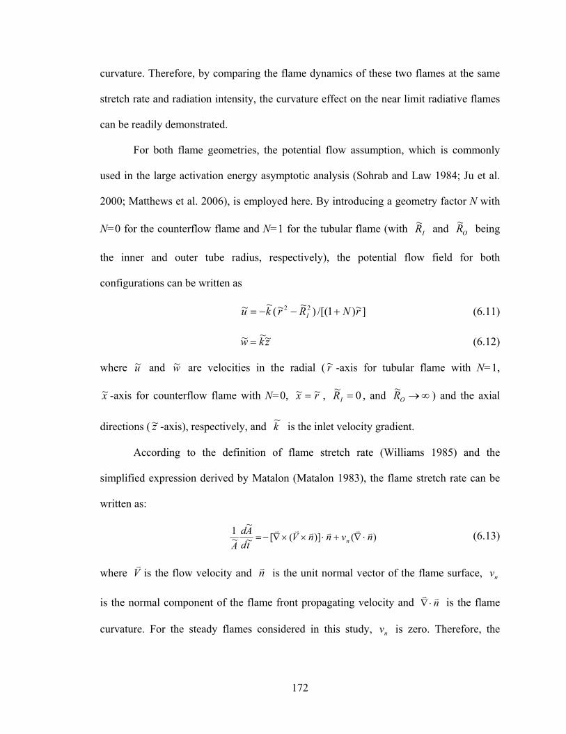
curvature. Therefore, by comparing the flame dynamics of these two flames at the same
stretch rate and radiation intensity, the curvature effect on the near limit radiative flames
can be readily demonstrated.
For both flame geometries, the potential flow assumption, which is commonly
used in the large activation energy asymptotic analysis (Sohrab and Law 1984; Ju et al.
2000; Matthews et al. 2006), is employed here. By introducing a geometry factor N with
N=0 for the counterflow flame and N=1 for the tubular flame (with IR~ and OR~ being
the inner and outer tube radius, respectively), the potential flow field for both
configurations can be written as
]~)1/[()~~(~~ 22 rNRrku I +−−= (6.11)
zkw ~~~ = (6.12)
where and are velocities in the radial (u~ w~ r~ -axis for tubular flame with N=1,
-axis for counterflow flame with N=0, x~ rx ~~ = , 0~ =IR , and ∞→OR~ ) and the axial
directions ( z~ -axis), respectively, and is the inlet velocity gradient. k~
According to the definition of flame stretch rate (Williams 1985) and the
simplified expression derived by Matalon (Matalon 1983), the flame stretch rate can be
written as:
)()]([~~
~1 nvnnV
tdAd
A nvvvvvv
⋅∇+⋅××∇−= (6.13)
where Vv
is the flow velocity and nv is the unit normal vector of the flame surface,
is the normal component of the flame front propagating velocity and is the flame
curvature. For the steady flames considered in this study, is zero. Therefore, the
nv
nvv
⋅∇
nv
172

stretch rate, which only depends on the flow field given by equations (6.11) and (6.12)
becomes
kurrd
drtd
AdA
NN
~)~~(~~1
~~
~1
=−= (6.14)
which indicates that the two flame configurations will have the same stretch rate if
the inlet velocity is specified according to equations (
k~
6.1) and (6.2). Note that the flame
stretch rate is independent of the inner tube radius k~ IR~ . Therefore, by fixing and
varying
k~
IR~ for the tubular flame configuration (N=1), flames at the same stretch rate
but different curvatures (different flame radii fR~ ) can be obtained (Takeno et al. 1986;
Kobayashi and Kitano 1989; Mosbacher et al. 2003; Yokomori et al. 2006). When
∞→IR~ and N=1, the tubular flame has zero flame curvature and it becomes
counterflow flame (N=0); when 0~ =IR and N=1, the flame curvature reaches its
maximum value and it is the traditional tubular flame configuration (without the inner
tube) employed in previous studies (Takeno and Ishizuka 1986; Takeno et al. 1986;
Nishioka et al. 1988; Kobayashi and Kitano 1989; Nishioka et al. 1991; Kobayashi and
Kitano 1993; Ju et al. 1999b; Matthews et al. 2006). Therefore the present model is more
general and it will be shown that previous results on both counterflow flames and tubular
flames can be recovered.
Since we are interested in the dynamics of the near-limit flames, the combustible
mixture is sufficiently off-stoichiometric so that the flame strength is only determined by
the concentration of the fuel. By assuming constant density, constant thermal properties,
and one-step irreversible chemical reaction, the nondimensional conservation equations
for energy and fuel mass fraction can be written as
173

rN
NI q
drdTr
drd
rdrdT
rRrk −+=
−− ω)(122
(6.15)
ω−=−
− )(1122
drdYr
drd
rLedrdY
rRrk N
NI (6.16)
Parameters with and without the carrot symbol denote the dimensional and
non-dimensional variables, respectively. The variables, r, T and Y are, respectively, the
axial coordinate, temperature, and fuel mass fraction normalized by 0~fδ , PCQY ~/~~
∞ , and
∞Y~ , where )~~~/(~~ 00LPf SCρλδ = is the flame thickness of adiabatic planar flame, the
thermal conductivity,
λ~
ρ~ the density, PC~ the specific heat capacity at constant
pressure, Q~ the reaction heat-release per unit mass of fuel, and ∞Y~ the fuel mass
fraction in the fresh mixture. Additionally, DCLe P~~~/~ ρλ= is the Lewis number and D~
the mass diffusivity of fuel. The normalized stretch rate is ]~)1/[()~(~~~ 20 λδρ += NCkk fP .
The adiabatic laminar burning velocity 0~LS for a first-order one-step reaction is
(Williams 1985):
2/1
20 )exp(~
~~
~2~
⎭⎬⎫
⎩⎨⎧
−⋅⋅⋅⋅=ad
a
PL T
TZLeB
CS
ρλ (6.17)
where is the Zeldovich number, 2/ ada TTZ = B~ the pre-factor of the Arrhenius
expression, Tad the normalized adiabatic flame temperature, and Ta the normalized
activation temperature.
On the right-hand side of equation (6.15), qr is the nondimensional volumetric
radiative heat loss. It is approximated by using the optically thin grey gas model of (Ju et
al. 1997)
174
)~~~/(~)~)(~~(~~4 2044 λδσ QYCTTKq PfPr ∞∞−= (6.18)
where σ~ is the Stefan-Boltzmann constant, pK~ the Planck mean absorption
coefficient of the mixture, and ∞T~ the temperature of the incoming fresh mixture.
In the limit of large activation energy, chemical reaction occurs only within a very
thin zone of high temperature, whose thickness is much smaller than that of the radiation
zone (Sohrab and Law 1984; Ju et al. 1997). Therefore, the reaction rate can be replaced
by the Dirac Delta function (Sivashinsky 1977; Joulin and Clavin 1979; Law 2006)
)()22
exp( ff
a
ad
a RrTT
TT
−⋅−= δω (6.19)
where Tf and Rf are the flame temperature and radius, respectively. By integrating the
conservation equations (6.15) and (6.16) around the flame front (r=Rf), the jump relations
for temperature and fuel mass fraction can be obtained as (Sivashinsky 1977; Joulin and
Clavin 1979)
)22
exp()(1
f
a
ad
a
RRRR TT
TT
drdY
drdY
LedrdT
drdT
ffff
−=−=−−++−
(6.20)
The symmetric (for RI=0) or adiabatic (for RI>0) condition is used at the inner
boundary (r=RI). At the inlet (r=RO), the Hirschfelder boundary condition for the fuel
concentration, as suggested by Matthews et al. (Matthews et al. 2006), is used instead of
the plug flow boundary condition. By defining the flame as the location where fuel
concentration goes to zero, the boundary conditions for temperature and fuel mass
fraction can be given as
rRrYkdrdYLeTTRr
YTTRrdrdYdrdTRr
IO
ff
I
/))(1(/,:
0,:0/,0/:
221 −−===
======
−∞
(6.21)
175

It should be noted that for the counterflow flame (R0→∞), the inlet boundary
condition (6.21c) reduces to the plug flow boundary condition (Y=1), which is used in
previous theoretical studies of counterflow flames (Ju et al. 2000).
In the limit of large activation energy, it is reasonable to assume that the
magnitude of the radiative loss term in the energy equation is one-order smaller than
those of the convection and diffusion terms. This assumption has been widely used in
combustion theory (Joulin and Clavin 1979; Buckmaster 1997) and its validity has been
confirmed by previous analysis. The radiation term given by equation (6.18) can be
written as
)( 44∞−= TThqr , 1)~~/(~~)~(~~4 33320 <<= ∞ PfP CQYKh λδσ (6.22)
The validity of h<<1 is shown in (Chen and Ju 2008). It is noted that the
nonlinear radiative heat loss is considered in the present study. It was shown by Ju et al.
(Ju et al. 2000) that the linearized radiative heat loss results in a narrower flammable
region and a larger flammability limit compared with the nonlinear radiative heat loss
model. Therefore, by using the nonlinear radiation model, the present model can more
accurately demonstrate the dynamics of radiation dominated near-limit flames.
Since the delta-function model for reaction rate is used here, in the limit of large
activation energy, the governing equations can be solved analytically in the burned gas
(RI ≤r≤ Rf) and unburned gas (Rf ≤r≤RO) regions separately. The fuel mass fraction in the
burned gas region is zero according to the fuel lean assumption and that in the unburned
gas region is obtained by solving equation (6.16) together with the boundary conditions
in equation (6.21), which gives
176
2/11222/
2/
2222
22
)]([)(
OIO
f
I
f
I
kLeRNkLeROIO
R
R
kLeNkLeR
r
R
kLeNkLeR
eRRRkLede
derY
−+−−−−
−−
+
−+=
∫∫
ττ
ττ
τ
τ
(6.23)
Here the superscripts ‘+’ and ‘−’ denote the states on the unburned and burned
sides of the flame front, respectively. To determine the temperature distribution, the
energy equation (6.15) with boundary conditions in equation (6.21) can be solved
asymptotically, i.e. T=T0+hT1+O(h2), with the accuracy to the first order, O(h). The
temperature distribution in the burned gas region (RI ≤ r ≤ Rf) is
( ) τττ τ∫ ∫ ⎥⎦
⎤⎢⎣⎡−−= −−
∞−− f
I
IR
r R
skkRNff ddsesTThTrT 2/)(44 222
/)()( (6.24)
and that in the unburned gas region (Rf ≤ r ≤ RO) is
)()()( 10 rThrTrT ++++ += (6.25)
)(/)()()(0 ff RGrGTTTrT ∞∞+ −+= (6.26)
dsdssdT
sTrTsdsdssdT
sTTsRGrGrT OO
f
R
r
R
R
f
f∫∫ +
++
+
++ −
−−
=/)(
)]()()[(/)(
)]()[()(
)()(0
00
0
01
ϕϕ (6.27)
where and . ττ τ∫ −−=O
IR
r
kNkR derG 2/22
)( 44)]([)(0 ∞+ −= TrTrϕ
The gradients of temperature and fuel mass fraction at the flame front can be
obtained from their distributions given by equations (6.23-6.27). By using the jump
relations in equation (6.20), one obtains the following algebraic system of equations for
the flame radius, Rf, and flame temperature, Tf
( )
),(),(/
),(2/)(
1222 ffffR
R
sRkNkRf
ff TRLTRL
dseRs
TTLeRFLe
O
f
fI
−+
−−
∞+− ++−
=⋅∫
(6.28)
2/)(111
),(−− −+− =⋅ fada TTT
f eLeRFLe (6.29)
177
where
2/11222/
2/
2222
22
)]([),(
OIO
f
I
fI
kLeRNkLeROIO
R
R
kLeNkLeR
kLeRNkLeRf
feRRRkLede
eRLeRF
−+−−−−
−−+
−+=
∫ ττ τ (6.30)
( )
( )∫∫ ∫
−−
−−
++ ⎥⎦⎤
⎢⎣⎡
=O
f
fI
O
f
O I
R
R
sRkNkRf
R
R
R skNkR
ffdseRs
ddseshTRL
2/)(
2/)(
222
222
/
/)(),(
τττϕτ
τ
(6.31)
( )∫ −−∞
−− ⋅−=f
I
fIR
R
RskkRNffff dseRsTThTRL 2/)(44 222
/)(),( (6.32)
Equations (6.28) and (6.29) yield a general solution for both tubular flames (N=1)
and counterflow flames (N=0). The solution for the flame radius, Rf, and flame
temperature, Tf, as a function of stretch rate, k, can be obtained by solving the above
equations numerically for different h, RI, RO, N and Le. The flame speed, which is equal
to the flow speed at the flame front, can be calculated from the flame radius and the
potential flow field given by equations (6.11) and (6.12). According to equation (6.29),
the term on the left-hand side of equation (6.28) denotes the total chemical heat release.
The first term on the right-hand side of equation (6.28) represents the heat flux induced
by thermal conduction to the unburned side, while the second and third terms represent
the heat flux induced by radiative loss in the unburned and burned regions, respectively.
The adiabatic flame temperature of stretched flames can be obtained by setting the
radiative loss terms (L± or h±) to zero.
Equations (6.28) and (6.29) reduce to previous results of adiabatic tubular flames
(Matthews et al. 2006) in the limit of N=1, RI=0, and L±=0; and those of counterflow
flames (Sohrab and Law 1984; Ju et al. 2000) in the limit of N=0, RI=0, and R0→∞.
Furthermore, by specifying RI>RO (now the outer tube is of radius RI while the inner one
of radius RO), solutions to tubular flames of negative curvature (unlike the tubular flame
178

of positive curvature shown in figure 6.14(a), a tubular flame of negative curvature is
established when combustible mixture is injected toward the outer tube through the
porous inner tube) can be obtained from the present results.
6.3.3 Results and Discussions
The present results, equations (6.28) and (6.29), provide a general theoretical
description of flame speed, flame temperature and extinction limits. By specifying
different flame curvatures (by changing RI or N), flame stretches (by changing k), and
radiative heat loss intensities (by changing fuel concentration or the concentrations of
radiative gases, h±), the effects of flame curvature, radiation, and stretch rates can be
systematically investigated. Furthermore, the preferential diffusion effect can be
demonstrated by comparing results at different Lewis numbers (by changing Le).
In the following calculations, the integrations in equations (6.28) and (6.29) are
evaluated by using QUADPACK (Piessens et al. 1983) and the thermal and chemical
parameters are chosen to mimic methane/air mixture. They are KgJQ /1075.4~ 7⋅= ,
KKgJCP //1400~ = , , smolmB //105.2~ 310⋅= 3/0.1~ mKg=ρ , KT 300~ =∞ ,
KTa 25000~ = , 10.2~ −= mK P , and smCP /105)~~/(~ 25−⋅=ρλ . The Lewis number of
methane/air flames is close to unity. Therefore, unit Lewis number is utilized in the
following except in the last subsection, in which the effects of Lewis number is
investigated and different Lewis numbers could be obtained by adding Helium into the
methane/air mixture (Chen et al. 2007a).
In the following, the effects of flame curvature, radiation, stretch, and Lewis
number on flame extinction will be discussed. Note that the outer tube radius is set to be
infinity (RO = ∞), so the heat conduction to the outer tube, which was studied by
179
Kobayashi et al. (Kobayashi and Kitano 1989) and Matthews et al. (Matthews et al.
2006), is not considered here. Besides, in the present study and all previous studies, the
surface radiation is not considered in the tubular geometry. The existence of the inner and
outer tubes could interact with the gas-phase radiation losses. This is a subject for future
study.
6.3.3.1 Flame Extinction and Bifurcations of Tubular Flames
It is well known that radiative heat loss depends strongly on the volume of the hot
emitting gas. Therefore, the appearance of flame curvature in tubular flame yields a
smaller volume of the burned gas per unit area of the flame front than that of the planar
counterflow flame. As a result, an increase of flame curvature reduces the radiative heat
loss and thus improves the combustion. On the other hand, an increase of flame curvature
increases the heat conduction loss from the burned gas side to the unburned gas side
(caused by the so-called defocusing effect) and the flame speed is decreased. So flame
curvature also weakens the flame strength. The above two competing effects of flame
curvature, together with that of radiation will be shown to greatly affect the flame
extinction.
To quantitatively evaluate the effect of radiative heat loss, the fraction of radiative
heat loss is introduced (Ju et al. 1997; Chen and Ju 2007):
⎥⎦⎤
⎢⎣⎡==
−− −
∫∫∫2/)( 11
)2(/)2()2(/)2( fadaO
I
O
I
O
I
TTTNf
R
R
Nr
R
R
NR
R
Nr eRdrrqdrrdrrqFr πππωπ (6.33)
where the numerator denotes the total radiative heat loss in both the unburned and burned
zones and the denominator denotes the total chemical heat release rate.
Figure 6.15 shows the dependences of flame radius, flame temperature and
fraction of radiative heat loss of tubular flames (RI=0, RO=∞, N=1) on stretch rate at
180

Le=1.0 and ∞Y~ = 0.0376. It is seen that the non-adiabatic tubular flames exhibit an isola
response, with dual extinction limits at higher and lower values of stretch rate (b and d).
According to previous stability analysis mentioned in (Matthews et al. 2006), the branch
of large flame radius (thus large flame speed) is stable (solid lines in figure 6.15) while
the branch of small flame radius (thus small flame speed) is unstable (dashed lines in
figure 6.15).
It is seen that the mixture can burn in a range of stretch rate between 1.3 s-1 and
6.7 s-1. For stretch rates larger than 3.5 s-1 (point a), an increase of the stretch rate causes
the decrease of flow residence time and flame radius. Therefore, the fraction of radiative
heat loss decreases and flame temperature increases. Flame extinction occurs at point b.
For counterflow flames, this extinction is usually called stretch-induced extinction limit
(Sohrab and Law 1984; Sung and Law 1996; Buckmaster 1997; Ju et al. 1997; Ju et al.
1999a; Ju et al. 2000). However, for tubular flames the flame curvature (inverse of flame
radius) reaches its maximum value at the extinction point b and thus the curvature effect
might also help to accelerate flame extinction. The validity of this conclusion will be
proved in the next section.
On the other hand, with the decrease of stretch rate (from point a to c to d), the
flow residence time increases, which enhances the radiative heat loss; while the flame
curvature also increases, which reduces radiation by decreasing the volume of radiation
emitting gas. The two processes compete with each other and result a non-monotonic
change of radiation fraction and flame temperature, as shown in figure 6.15. From point a
to c, the effect of residence time dominates and thus radiation fraction increases and
flame temperature decreases; from point c to d, the effect of curvature dominates and thus
181

radiation fraction decreases and flame temperature increases. The flame is eventually
quenched at point d. Therefore, unlike the counterflow flame whose low stretch rate
extinction limit is only caused by an increase of radiation, that of tubular flame is caused
by the combined effects of flame curvature and radiation. Therefore, both the stretch and
radiation extinction limits of tubular flames are strongly affected by flame curvature.
Results of tubular flames at other fuel concentrations ( ∞Y~ = 0.0392, 0.04) are
shown in figure 6.16 in order to demonstrate the effect of different radiation intensities (h
= 0.017, 0.011, 0.009 for ∞Y~ = 0.0376, 0.0392, 0.04, respectively). Different flame
regimes are predicted. For ∞Y~ = 0.0376, the flammable region is an isola with flame
position near the stagnation line (r=0). This is usually called Near Stagnation Flame
(NSF). However, with the increase of fuel concentration and thus decrease of radiative
heat loss intensity, figure 6.16 shows that there are two distinct flame branches for ∞Y~ =
0.0392: one branch is a NSF similar to that of ∞Y~ = 0.0376, the other one is far from the
stagnation line and thus is called a FSF. For both branches, the sold lines stand for stable
solutions while the dashed lines are unstable solutions. With the decrease of radiative
heat loss intensity h (or increase of ∞Y~ ), the flame can survive radiation from emitting
volume much larger than that of NSF, which is the reason why the FSF appears. With
further decrease of radiative heat loss intensity, the strength of FSF increases and its
extinction limit moves to the higher stretch rate side. At the same time, the NSF is also
strengthened and it can survive despite the larger radiation emitting volume (thus large
fR~ ). Therefore, flame branch bifurcations appear with the increase of fuel concentration
(decrease of radiative heat loss intensity). Figure 6.16 shows that, for ∞Y~ = 0.04, the FSF
182
branch ag and NSF branch hb merge with each other to form branch ab, and so do the
FSF branch fg and NSF branch hd to form branch fed. It is seen that for ∞Y~ = 0.04 there
are two stable solutions for stretch rate between 0.33 s-1 and 2.72 s-1, of which the one of
higher temperature (on ab branch) is call normal flame, while the one of lower
temperature (on de branch) is called the weak flame (Ju et al. 1999a; Ju et al. 1999b).
Similar flame bifurcations shown in figure 6.16 have also been found in the
detailed numerical simulation of tubular and counterflow methane-air flames (Ju et al.
1997; Ju et al. 1999b) and theoretical analysis of counterflow flames (Buckmaster 1997),
which confirms the validity of the present general theoretical description of the combined
effects of flame curvature, radiation, and stretch given by equations (6.28) and (6.29).
The different flame regions of counterflow flames predicted by the present theoretical
correlation is the same as those shown in Buckmaster’s analysis (Buckmaster 1997) and
thus are not repeated here.
6.3.3.2 Curvature and Radiation Effects on Extinction Limits
To further study the combined effect of flame curvature and radiation, the tubular
flames of different inner tube radii IR~ are studied for mixture of Le=1.0 and ∞Y~ =
0.0376. The dependence of flame position (stable branches in solid lines and unstable
branches in dashed lines) and flame temperature (only stable branches) on stretch rate are
shown in figure 6.17. It is seen that by continuously increasing the inner tube radius, the
isola response for counterflow flames is recovered. Note that the flame position If RR ~~ −
and the flame temperature are strongly affected by the inner tube size. Flame position
If RR ~~ − and flame temperature both increase with the increase of flame curvature
(decrease of IR~ ) since flame curvature reduces the radiative heat loss.
183

Furthermore, the flame position, flame temperature, and stretch rate at both
extinction limits are significantly changed by choosing different inner tube radii. As
shown in figure 6.18, the stretch rate at the upper extinction limit (stretch extinction limit)
decreases monotonically with the increase of flame curvature (decrease of the inner tube
radius). However, it is interesting to note that the dependence of the lower extinction
limit (radiation extinction limit) on flame curvature is not monotonic. Similar
non-monotonic dependences for flame position and flame temperature on flame curvature
at the radiation extinction limits can also be seen in figure 6.17. This result shows that
flame curvature and radiation coupling has distinct effects on the stretch extinction limit
and the radiation extinction limit.
For extinction at high stretch rate, when the inner tube radius is large, flame is
very close to the stagnation surface ( 0~~ ≈− If RR for IR~ =1, 5 mm in figure 6.17) and
the radiation fraction reaches its minimum value (according to figure 6.15(3)). So the
radiation effect at upper extinction limit could be negligible. This is further confirmed by
the nearly constant flame temperature at the stretch extinction limit for different IR~
shown in figure 6.17. Therefore, the change of extinction stretch rate is purely caused by
flame curvature. When the inner tube radius is smaller than 1 mm, the If RR ~~ − at
extinction increases significantly with decrease of IR~ , and then flame temperature
decreases because of the increase of radiative heat loss. Therefore, the change of
extinction stretch rate is caused by combined effects of flame curvature and radiation.
For extinction at low stretch rate, flame extinction is also caused by the combined
effects of flame curvature and radiation. As mentioned before, an increase of flame
curvature has two effects: (1), the reduction of the radiative heat loss and consequent
184
improvement in combustion; and (2), the decrease of flame speed and consequent
reduction in the flame strength. The two processes compete with each other in the
determination of the low stretch rate extinction limits. For large inner tube radius
( IR~ >1.6 mm), the first effect dominates, thus the stretch rate at extinction decreases with
the increase of flame curvature (decrease of inner tube size); while for small inner tube
radius ( IR~ <1.6 mm), the second effect dominates, thus the stretch rate at extinction
increases with the increase of flame curvature (decrease of inner tube size).
Therefore, flame curvature has significant effects on extinction of premixed
tubular flames since the extinction limits can be greatly changed by choosing different
inner tubes to change flame curvature. Note that all the cases studied above are for
mixtures of Le=1.0, so the stretch effect caused by preferential diffusion is not covered.
The Lewis number effect will be demonstrated in the next section.
6.3.3.3 Effects of Preferential Diffusion (Lewis Number Effect)
The impact of radiation and flame curvature coupling on near limit flames will be
enriched by the appearance of preferential diffusion. The effects of Lewis number on the
tubular flames are shown in figure 6.19. It can be seen that the flammable region is
greatly expanded by decrease of Lewis number. With decrease in the Lewis number, the
stretch rate at upper limit increases while that at lower limit decreases. Furthermore, the
flame radius decreases and flame temperature increases with the decrease of Lewis
number at both extinction limits. This effect can be easily understood from equations
(6.28) and (6.29). Equations (6.28) and (6.29) shows that the lower the Lewis number, the
higher the adiabatic flame temperature and thus flame can survive much larger radiative
heat loss and flame curvature. Note that the flame temperature increase at upper
185
extinction limit is much larger than that at lower extinction limit. This is because the
Lewis number effect is proportional to the magnitude of stretch rate. Similar results for
counterflow flames are also obtained from the present theory and are consistent with
those of the previous study (Ju et al. 2000).
To demonstrate further the effects of Lewis number, radiation, and curvature on
the extinction of tubular flames, the stretch rates at two different extinction limits for
different inner tube radii and Lewis numbers are shown in figure 6.20. For fixed inner
tube radius, the Lewis number effect is the same: the stretch rate at the upper limit
increases while that at the lower limit decreases with decreasing Lewis number.
Therefore, the preferential diffusion of mass over heat (Le<1) extends the flammable
region for all the tubular flames with different curvatures. For fixed Lewis number, the
stretch rate at the upper stretch extinction limit decreases monotonically. However,
depending on the Lewis number, the radiation extinction limit can be either
monotonically or non-monotonically dependent on the flame curvature. At large Lewis
numbers (e.g. Le=1.1), the stretch effect is dominant. Therefore, an increase of flame
curvature leads to a monotonical increase of the extinction limit. There is a critical
curvature above which no premixed tubular flames can be obtained (for Le=1.1, no
solution for RI<1.5 mm). However, at lower Lewis numbers (e.g. Le=0.9 and 1.0), the
effect of radiation and flame curvature coupling becomes dominant. The radiation
extinction limit varies non-monotonically with the flame curvature. In addition, flame
curvature does not lead to flame extinction. As shown in figure 6.20, at a large flame
radius, the decrease of the flame radius causes a decrease (or broadening) of the
extinction limit. As the flame curvature increases, the radiation extinction limit reaches a
186

minimum value. A further increase of the flame curvature causes an increase of the
extinction limit. Therefore, there is a critical Lewis number that separates the monotonic
and nonmonotonic curvature dependence regimes. This critical Lewis number will be
larger than unity and increases with increasing radiation intensity.
6.3.4 Summary
The flame dynamics of near-limit premixed tubular flames are studied by using
the large activation energy asymptotic method. A general correlation for flame speed,
flame temperature and extinction limits is obtained and it is used to study the combined
effects of flame curvature, radiation, and stretch on flame extinction. The following
conclusions are made:
1. The coupling between radiation and flame curvature leads to multiple flame
bifurcations and extinction limits at different radiation intensities (different fuel mass
concentrations). For mixtures with high radiation intensity, the flammable region is an
isola and only the NSF is observed. With decreasing radiative loss intensity, two distinct
flame branches NSF and FSF are first predicted and then they will merge with each other.
2. It is shown that both the stretch and radiation extinction limits are strongly
affected by flame curvature. The stretch extinction limit is found to monotonically
decrease with increasing flame curvature. However, depending on the Lewis number, the
radiation extinction limit can be either monotonically or non-monotonically dependent on
the flame curvature. For Lewis numbers larger than a critical value, increasing flame
curvature results in a monotonic increase of the extinction limit and there is a critical
curvature at which flame extinguishes. For Lewis numbers smaller than the critical value,
187
increasing flame curvature leads to a non-monotonic dependence of the radiation
extinction limit and flame curvature does not lead to flame extinction.
188

burned gases
burned gases
OPF IPF
Figure 6.1: The schematic diagrams of (a) the outwardly propagating spherical flame
(OPF) and (b) the inwardly propagating spherical flame (IPF) (Frankel and Sivashinsky
1983).
Flame radius, R
Flam
epr
opag
atin
gsp
eed,
U
10 30 50 70 90 110 130 1500.0
0.5
1.0
1.5
Flame radius, R
Flam
epr
opag
atin
gsp
eed,
U
10 30 50 70 90 110 130 1500.0
0.5
1.0
1.5
Le=1.0
Le=2.0
Le=0.5L=0.0
L=0.1
solid lines: detailed modeldashed lines: simplified model
Figure 6.2: The flame propagation speed as a function of flame radius for OPF predicted
by different models.
189
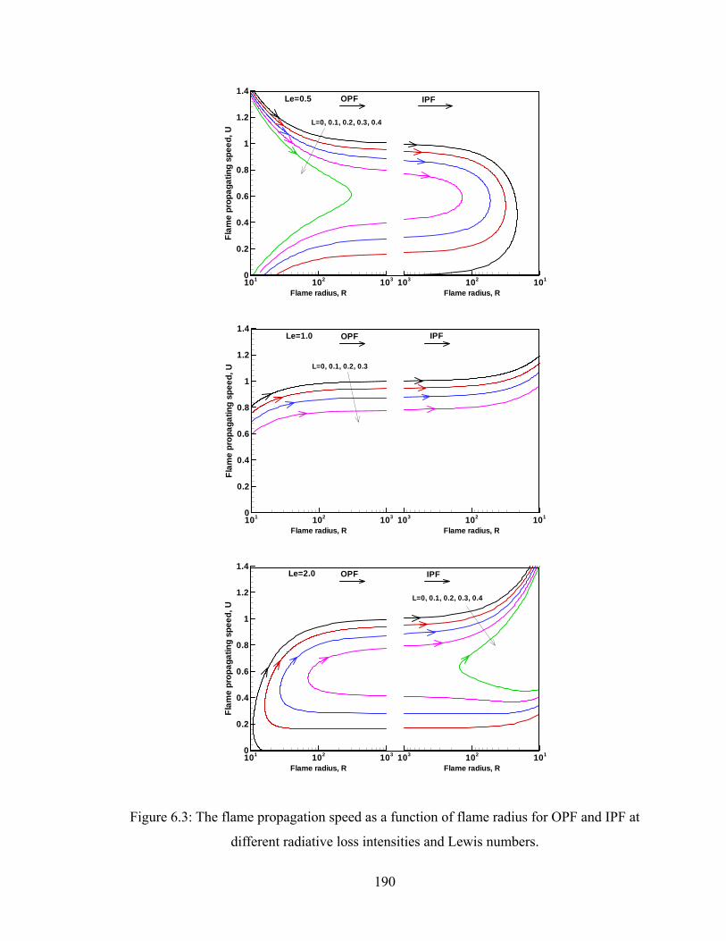
Flame radius, R
Flam
epr
opag
atin
gsp
eed,
U
101 102 1030
0.2
0.4
0.6
0.8
1
1.2
1.4OPF
L=0, 0.1, 0.2, 0.3, 0.4
Le=0.5
Flame radius, R101102103
IPF
Flame radius, R
Flam
epr
opag
atin
gsp
eed,
U
101 102 1030
0.2
0.4
0.6
0.8
1
1.2
1.4OPF
L=0, 0.1, 0.2, 0.3
Le=1.0
Flame radius, R101102103
IPF
Flame radius, R
Flam
epr
opag
atin
gsp
eed,
U
101 102 1030
0.2
0.4
0.6
0.8
1
1.2
1.4OPFLe=2.0
Flame radius, R101102103
IPF
L=0, 0.1, 0.2, 0.3, 0.4
Figure 6.3: The flame propagation speed as a function of flame radius for OPF and IPF at
different radiative loss intensities and Lewis numbers.
190

Karlovitz number, K
Flam
epr
opag
atin
gsp
eed,
U
-0.1 -0.05 0 0.05 0.10
0.2
0.4
0.6
0.8
1
1.2
1.4
Le=0.5IPF OPF
L=0, 0.1, 0.2,0.3, 0.4
Karlovitz number, K
Flam
epr
opag
atin
gsp
eed,
U
-0.1 -0.05 0 0.05 0.10
0.2
0.4
0.6
0.8
1
1.2
1.4
Le=1.0IPF OPF
L=0, 0.1, 0.2, 0.3
Karlovitz number, K
Flam
epr
opag
atin
gsp
eed,
U
-0.1 -0.05 0 0.05 0.10
0.2
0.4
0.6
0.8
1
1.2
1.4
Karlovitz number, K
Flam
epr
opag
atin
gsp
eed,
U
-0.1 -0.05 0 0.05 0.10
0.2
0.4
0.6
0.8
1
1.2
1.4
Le=2.0IPF OPF
L=0, 0.1,0.2, 0.3, 0.4
Figure 6.4: The flame propagation speed as a function of Karlovitz number for OPF and
IPF at different radiative loss intensities and Lewis numbers.
191
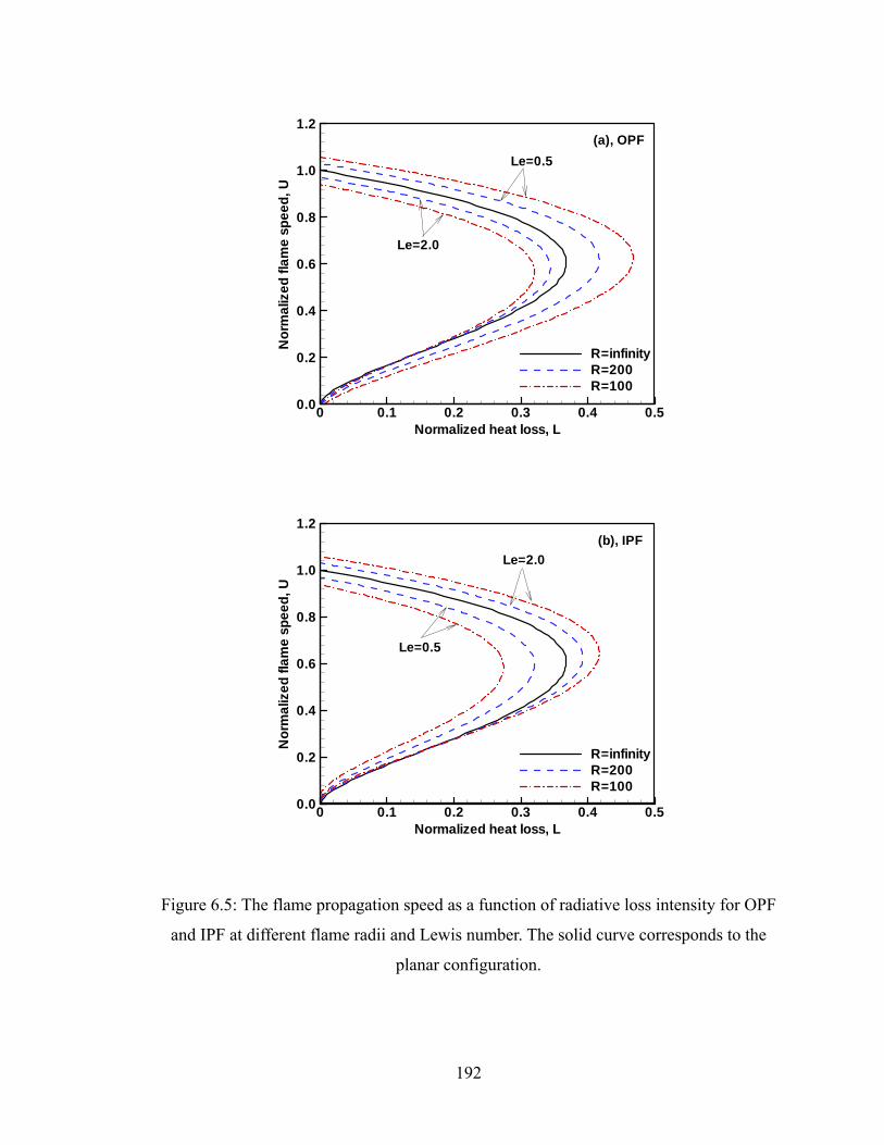
Normalized heat loss, L
Nor
mal
ized
flam
esp
eed,
U
0 0.1 0.2 0.3 0.4 0.50.0
0.2
0.4
0.6
0.8
1.0
1.2
R=infinityR=200R=100
Le=0.5
Le=2.0
(a), OPF
Normalized heat loss, L
Nor
mal
ized
flam
esp
eed,
U
0 0.1 0.2 0.3 0.4 0.50.0
0.2
0.4
0.6
0.8
1.0
1.2
R=infinityR=200R=100
Le=0.5
Le=2.0(b), IPF
Figure 6.5: The flame propagation speed as a function of radiative loss intensity for OPF
and IPF at different flame radii and Lewis number. The solid curve corresponds to the
planar configuration.
192
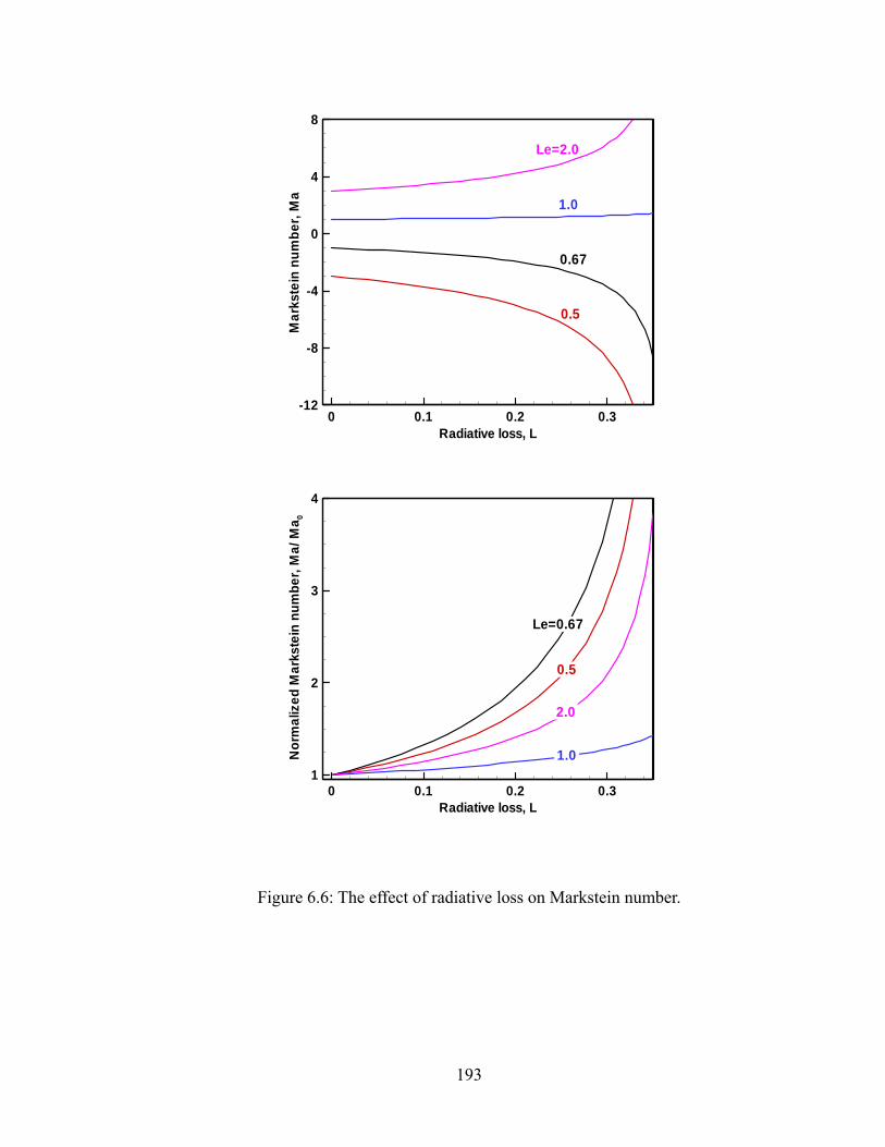
Radiative loss, L
Mar
kste
innu
mbe
r,M
a
0 0.1 0.2 0.3-12
-8
-4
0
4
8
0.67
1.0
Le=2.0
0.5
Radiative loss, L
Nor
mal
ized
Mar
kste
innu
mbe
r,M
a/M
a 0
0 0.1 0.2 0.31
2
3
4
Le=0.67
0.5
2.0
1.0
Figure 6.6: The effect of radiative loss on Markstein number.
193

Lewis number, Le
Nor
mal
ized
Mar
kste
innu
mbe
r,M
a/M
a 0
0 0.5 1 1.5-2
-1
0
1
2
3
4
5
L=0.0L=0.1L=0.2L=0.3
2
Le=0.8Ma0=0
Figure 6.7: The normalized Markstein number as a function of Lewis number at different
radiative losses.
Figure 6.8: Schlieren photographs of CH4-(0.3O2+0.2He+0.5CO2) flames at different
equivalence ratios at 1 atm.
194

0.3 0.4 0.5 0.6 0.7 0.80
10
20
30
Experiment SNB-GB1D FSNB-CK OPTM
Lam
inar
Fla
me
Spee
d, S
L (cm
/s)
Equivalence Ratio, ϕ
P=1 atm
Figure 6.9: Measured and predicted laminar flame speeds of CH4-(0.3O2+0.2He+0.5CO2)
flames as a function of equivalence ratio at 1 atm.
Spatial Coordinate r (cm)
Rad
iativ
eP
ower
(W/m
3 )
Tem
pera
ture
(K)
0 1 2 3 4 5 6-1.8E+07
-1.2E+07
-6E+06
0
6E+06
1.2E+07
0
500
1000
1500
2000
2500
3000
3500
4000
4500
5000ADIOPTMSNBGB-1DFSNB-CK(planar)FSNB-CK(spherical)
Figure 6.10: Temperature and volumetric heat loss distributions in spherical
CH4-(0.3O2+0.2He+0.5CO2) flame at φ=0.6 and P=1 atm.
195

0.3 0.4 0.5 0.6 0.7 0.80
5
10
15
20
25
Experiment SNB-GB1D FSNB-CK OPTM
Lam
inar
Fla
me
Spee
d, S
L (cm
/s)
Equivalence Ratio, ϕ
P=2 atm
0.3 0.4 0.5 0.6 0.7 0.80
5
10
15 Experiment SNB-GB1D FSNB-CK OPTM
Lam
inar
Fla
me
Spee
d, S
L (cm
/s)
Equivalence Ratio, ϕ
P=5 atm
Figure 6.11: Measured and predicted laminar flame speeds of CH4-(0.3O2+0.2He+0.5CO2)
flames as a function of equivalence ratio at 2 atm and 5 atm.
196

1 2 3 4 50.1
0.2
0.3
0.4
0.5 ϕ=0.6 ϕ=0.7 ϕ=0.8
(SL,
FSN
B-S L
,OPT
M)/S
L,O
PTM
Pressure (atm)
Figure 6.12: Effects of radiation absorption on flame speed at different pressure and
equivalence ratios.
0 1 2 3
-0.08
-0.04
0.00
0.04
B
B
Theory FSNB-CK OPTM
Effe
ctiv
e B
oltz
man
n N
umbe
r, B
Flame location, rf (cm)
CH4+{0.5CO2+0.2He+0.3O2}P=1 atm, T=298 K, ϕ=0.8
B/200
Figure 6.13: The predicted effective Boltzmann number versus flame size at 1 atm.
197

Figure 6.14: The schematic diagrams of the (a) tubular and (b) counterflow flames.
Stretch rate, k (1/s)
Frac
tion
ofra
diat
ion
heat
loss
,Fr
1 2 3 4 5 60.05
0.1
0.15
d
a
b
c (3)
∼ 7
Flam
era
dius
,Rf(m
)
0.001
0.002
0.003
d
a
b
c
(1)
∼Fl
ame
tem
pera
ture
,Tf(K
)
1400
1450
1500
da
b
c(2)
∼
Figure 6.15: Dependences of flame radius (1), flame temperature (2), and fraction of
radiative heat loss (3) of tubular flames (RI=0, RO=∞, N=1) on stretch rate for mixture of
Le=1.0 and ∞Y~ =0.0376.
Rf
flame
RO
z RI
O
r ~ ~
~
~ ~
(a) x
z
(b)
flame
flame
~
198
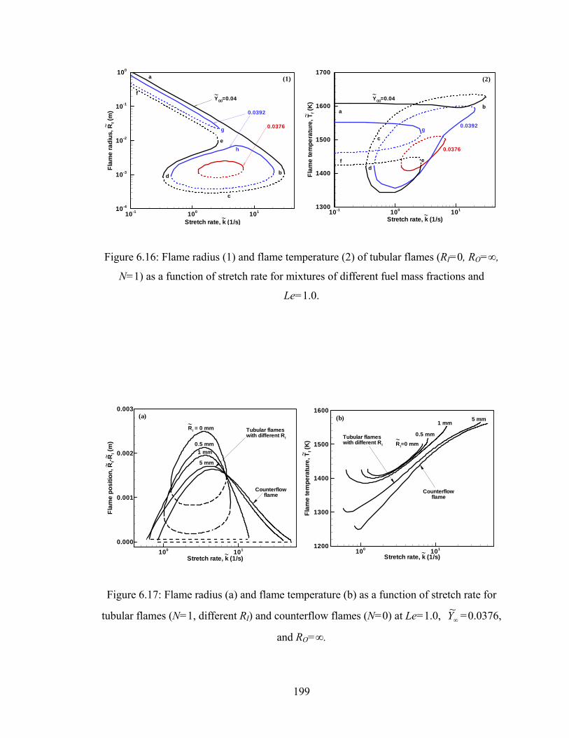
Stretch rate, k (1/s)
Flam
era
dius
,Rf(m
)
10-1 100 10110-4
10-3
10-2
10-1
100
Stretch rate, k (1/s)
Flam
ete
mpe
ratu
re,T
f(K
)
10-1 100 1011300
1400
1500
1600
1700
0.0376
0.0392
YO =0.04O
a
bd
e
f
g
h
c
∼
∼
(1)
∼
0.0376
0.0392
YO =0.04O
ab
def
gc
∼
∼
(2)
∼
Figure 6.16: Flame radius (1) and flame temperature (2) of tubular flames (RI=0, RO=∞,
N=1) as a function of stretch rate for mixtures of different fuel mass fractions and
Le=1.0.
Stretch rate, k (1/s)
Flam
epo
sitio
n,R
f-RI(m
)
100 101
0.000
0.001
0.002
0.003
Tubular flameswith different RI
Counterflowflame
RI = 0 mm
0.5 mm1 mm
5 mm
∼
∼∼
∼
(a)
Stretch rate, k (1/s)
Flam
ete
mpe
ratu
re,T
f(K
)
100 1011200
1300
1400
1500
1600
Tubular flameswith different RI
Counterflowflame
RI=0 mm
0.5 mm
1 mm5 mm
∼
∼
∼
(b)
Figure 6.17: Flame radius (a) and flame temperature (b) as a function of stretch rate for
tubular flames (N=1, different RI) and counterflow flames (N=0) at Le=1.0, ∞Y~ =0.0376,
and RO=∞.
199
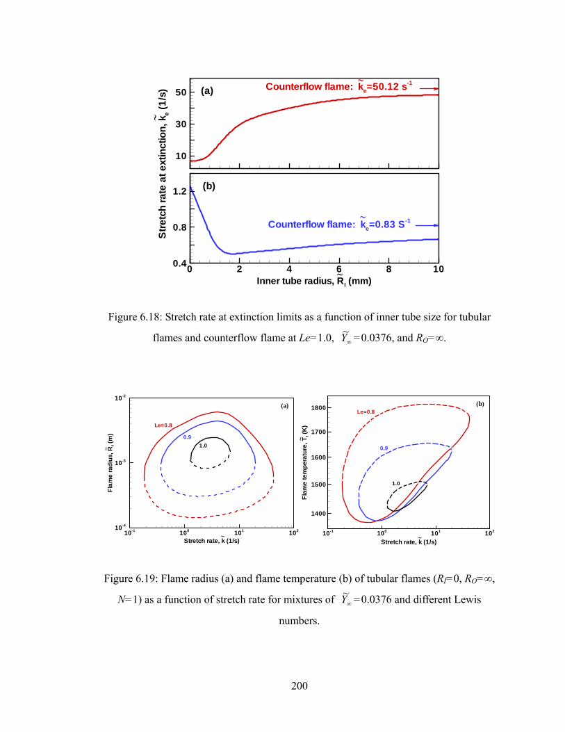
10
30
50 Counterflow flame: ke=50.12 s-1∼(a)
Inner tube radius, RI (mm)0 2 4 6 8 100.4
0.8
1.2
Stre
tch
rate
atex
tinct
ion,
k e(1
/s)
Counterflow flame: ke=0.83 S-1
(b)
∼
∼
∼
Figure 6.18: Stretch rate at extinction limits as a function of inner tube size for tubular
flames and counterflow flame at Le=1.0, ∞Y~ =0.0376, and RO=∞.
Stretch rate, k (1/s)
Flam
era
dius
,Rf(m
)
10-1 100 101 10210-4
10-3
10-2
Stretch rate, k (1/s)
Flam
ete
mpe
ratu
re,T
f(K
)
10-1 100 101 102
1400
1500
1600
1700
1800
1.0
Le=0.8
0.91.0∼
∼
(a)Le=0.8
0.9
∼
∼
(b)
Figure 6.19: Flame radius (a) and flame temperature (b) of tubular flames (RI=0, RO=∞,
N=1) as a function of stretch rate for mixtures of ∞Y~ =0.0376 and different Lewis
numbers.
200

Inner tube radius, RI (mm)
Stre
tch
rate
atex
tinct
ion,
k e(1
/s)
0 2 4 6 810-1
100
101
102
Le = 1.1
1.0
10
1.0extinction limit at large stretch rate
extinction limit at low stretch rate
∼
∼
0.9
0.9
Figure 6.20: Stretch rate at extinction limits as a function of inner tube size for tubular
flames at ∞Y~ =0.0376, and RO=∞.
201
Chapter 7: Ignition and Burning Properties of
DME/methane Mixtures
In previous chapters, the ignition and burning properties of different fuel/air
mixtures were studied. The transport effects on the flame dynamics were emphasized
while the chemical kinetic effect was covered. In this chapter, we shall demonstrate the
potential role of chemical kinetics on the ignition and burning intensity of flames by
using dimethyl ether/methane mixtures as an example.
7.1 Introduction
The objective of the present study is to investigate kinetic coupling effects of
DME addition on the high-temperature ignition and burning properties of methane–air
mixtures. First, experimentally measured laminar flame speeds of DME-air and CH4-air
mixtures are compared with predictions by different existing DME mechanisms including
a recently developed high temperature model by Zhao et al. (Zhao et al. 2008). This
mechanism is then used to study the effects of DME addition on the ignition
enhancement in both homogeneous and non-homogeneous systems. Finally, the flame
speeds of DME/CH4-air mixtures were measured using outwardly propagating spherical
flames. The results are compared with model predictions and the effect of kinetic
coupling on the burned Markstein length is discussed.
7.2 Experimental/numerical Specifications and Kinetic Model Selection
The laminar flame speed and Markstein length of DME/CH4-air premixed flames
were measured by using outwardly propagating spherical flames in the dual-chambered,
202

pressure-release-type, high pressure combustion chamber (Qin and Ju 2005).
Pre-mixtures were prepared by using the partial pressure method from pure methane and
DME compressed gas sources. The purities of the DME and CH4 were 99.8% and 99.9%,
respectively. Experiments were conducted for DME/CH4-air mixtures: (αCH3OCH3 +
(1-α)CH4 + air), with values of the volume fraction, α, ranging from zero to unity. The
combustible mixture was spark-ignited at the center of the chamber with the minimum
ignition energy so as to preclude significant ignition disturbances. The flame propagation
sequence was imaged by using Schlieren photography. A high-speed digital video camera
operating at 8000 frames per second was used to record the propagating flame images.
The stretched flame speed was first obtained from the flame history and then linearly
extrapolated to zero stretch rate to obtain the unstretched flame speed. The results
presented here are the averaged value of at least two tests for each experimental condition.
All experiments were performed at an initial temperature of 298±3 K and atmospheric
pressure. In order to examine the available kinetic mechanisms, the measured flame
speeds were compared with the numerical results obtained using PREMIX (Kee et al.
1985). Furthermore, A-SURF is utilized to carry out simulations of outwardly
propagating spherical DME/methane/air flames at atmospheric and elevated pressures.
The laminar flame speed and burned Markstein length were obtained from numerical
simulations.
The effect of adding DME on the ignition enhancement of methane was
investigated numerically in two different systems, a homogeneous flame configuration to
examine the kinetic ignition enhancement, and a nonpremixed counterflow configuration
to examine the effect of transport. The ignition time of homogeneous mixtures at constant
203
pressure and enthalpy was calculated by using SENKIN (Lutz et al. 1987). For the
nonpremixed simulations, the quasi-steady temperature and species distributions of
counter flowing DME/CH4 (298 K at the boundary) and hot air jets (1400 K at the
boundary) were determined under a frozen flow constraint. At time zero, chemical
reactions were allowed in the pre-calculated frozen flow field. Ignition time was recorded
when the first increase in the temperature field exceeded 400 K, indicating thermal
runaway. Simulations were conducted using an unsteady potential counterflow flame
code described by Ju et al. (Ju et al. 1997). To further examine the effect of flow
residence time on ignition enhancement, the stretch rate in the frozen flow configuration
was varied from low stretch to that near the ignition limit.
In order to properly model and interpret the present work, the chemical kinetic
model used in the calculations must be capable of predicting the pure fuel–air laminar
flame speed and high temperature shock tube ignition properties. One might expect that
comprehensively developed detailed mechanisms for DME oxidation would also be
capable of predicting high temperature kinetic properties for methane oxidation. The
measured laminar flame speeds of pure DME-air and CH4-air mixtures at atmospheric
pressure and room temperature are shown in figures 7.1 and 7.2, respectively, along with
the predictions utilizing a number of different DME mechanisms.
It is seen that the earlier DME mechanisms published by Curran and co-workers
(Curran et al. 1998; Curran et al. 2000; Fischer et al. 2000; Zheng et al. 2005)
(2000-Mech and 2003-Mech) are not able to well reproduce the measured flame speeds
for both lean and rich mixtures. Although a more recently updated version (Curran 2005),
2005-Mech, predicts flame speeds much better than the previous ones, there is still a
204
large discrepancy for lean DME–air and CH4–air flames. Recently, a new
high-temperature model that includes the revised decomposition parameters, updates in
the sub-model and thermo-chemistry for the hydrogen oxidation, and a revised C1-C2
species sub-model developed in recent experimental and modelling studies on ethanol
pyrolysis and oxidation, has been developed (Zhao et al. 2008). The mechanism was
constructed and tested hierarchically against a large volume of high temperature
experimental data for hydrogen, carbon monoxide, formaldehyde, and methanol
oxidation. The new high-temperature DME reaction mechanism (denoted here as
2008-Mech) consists of 263 reversible elementary reactions and 46 species, and its
predictions compare well with the high-temperature flow reactor data for DME pyrolysis
and oxidation, for oxidation at high temperatures in a jet-stirred reactor, for
high-temperature shock tube ignition, for species profiles from burner-stabilized flames
and for laminar flame speeds of DME–air flame (figure 7.1). The model also results in
excellent prediction of CH4-air flame speed data (figure 7.2). On the basis of the ability to
reproduce these same reference conditions, we utilize the 2008-Mech in the remainder of
comparisons reported in this chapter.
7.3 Results and Discussions
7.3.1 Ignition Enhancement by DME Addition
Figure 7.3 shows the effects of DME and hydrogen addition on the ignition delay
of homogeneous DME/CH4–air and H2/CH4–air mixtures. The results show that the
addition of DME to CH4–air has a dramatic enhancement in CH4–air ignition, particularly,
at small amounts of DME addition. It is seen that for 10% of DME addition, the ignition
time can be reduced by at least an order of magnitude. As the DME addition level reaches
205
40%, a further increase in DME blending has little effect on reducing the ignition time. It
is noted that the enhancement due to DME addition can be much larger than that of
hydrogen addition, given that the volume fraction of the added fuel is below 70%.
In order to understand the factors involved in the enhancement of methane
ignition by DME addition, radical path analysis was conducted. Figures 7.4 and 7.5 show
the radical pool development and CH3-reaction path analysis during the ignition of
DME/CH4-air mixtures for 0% and 10% (in volume) DME addition, respectively (the
contribution to d[CH3]/dt by the ith reaction is defined as the generation or production rate
of CH3 due to ith reaction, i
dtCHd /][ 3 , normalized by the summation of the absolute
value due to all the reactions, ∑i
idtCHd /][ 3 ). It is seen that addition of 10% DME
drastically increases the radical pool concentration growth. As the DME concentration
further increases, however, this effect is lessened which gives rise to the nonlinear
ignition enhancement observed in figure 7.3 (more results on radical pool development
and sensitivity analysis are shown in figures 4 and 5 in (Chen et al. 2007c)).
For CH4–air mixtures without DME, figure 7.4, the initial radical production is
governed by the reaction CH4+O2→CH3+HO2, which has no significant contribution to
the radical pool growth later in the induction period. The methyl radicals formed react
with O2 to yield CH2O and OH, or CH3O and O, with CH3O decomposing to form CH2O
and H. Through abstraction reactions, CH2O forms HCO which subsequently yields HO2
and CO through oxidation. The recombination reaction 2CH3(+M)→C2H6(+M) is the
main channel opposing the initial radical pool growth. When both CH3 and HO2 are
available in sufficient concentrations, CH3+HO2→CH3O+OH becomes an important
radical source. The above processes all depend on developing a significant pool of CH3
206
and HO2 before radical pool growth of OH, O, and H can occur. Since the governing
reaction CH4+O2→CH3+HO2 is slow relative to the similar reaction and/or thermal
decomposition rates of higher alkanes, the ignition time for pure CH4–air mixtures is, in
comparison, relatively longer.
Once a small amount of DME is present, the system is strongly driven by the
unimolecular decomposition of DME (figure 7.5). This reaction is the major initial source
of radicals and continues to contribute to radical production thereafter. With DME
addition to methane, the radical pool growth occurs much more rapidly (figure 7.5), as it
is not limited by the rate with which methyl radicals alone can produce more reactive
species. In the case of DME addition, unimolecular decomposition yields CH3O and CH3
at the above temperatures, and subsequent abstraction reactions of CH3 and radicals
generated from CH3O produce CH3OCH2 which in turn yields additional radical growth
through decomposition to CH3 and CH2O. These reaction sequences lead to a relatively
large concentration of HO2, which in turn provides an alternative mechanism for CH3 to
yield radicals (CH3+HO2 vs. CH3+O2). CH2O reacts with OH, H or CH3 through
CH2O+X→HCO+HX (X = OH, O, H, CH3). Formyl radicals further oxidize to produce
CO and HO2. CH3O decomposes through CH3O+M→CH2O+H+M, or reacts with O2 to
obtain CH2O and HO2. Moreover, the large concentrations of HO2 also produce H2O2 and
subsequent production of OH through H2O2+M→OH+OH+M. Thus, by adding DME to
methane not only is CH3 more easily generated, other sources and channels are also
available for generating radicals, as a result it enhances ignition.
Figure 7.6 shows the evolution of temperature and H-radical mass fraction in
nonpremixed ignition. The ignition kernel is seen to develop on the hot air side (the
207

stagnation plane is located at x=2.26 cm). The effect of DME addition on the ignition
time in nonpremixed counterflow systems is shown in figure 7.7. It is seen that, unlike
the homogenous case, the ignition enhancement strongly depends on the stretch rate. At
large stretch rates, the ignition is kinetically limited (the characteristic transport time is
shorter than that of ignition) so that a small amount of DME addition causes a rapid
reduction of the ignition time. For example, at a high stretch rate (a = 300 s-1), the short
flow residence time prevents the slow radical process from quickly building up the
radical pool, so that the ignition time of pure methane in nonpremixed counterflow is
considerably long. It is a kinetic limited process. However, at low stretch rates, the
ignition time is limited by the characteristic transport time (transport limited). In this
regime, the ignition time only slightly decreases with increasing DME concentration.
Furthermore, it is noted that for both low and high stretch rates, the minimum ignition
times for large amounts of DME addition are of the same order, indicating the limiting by
transport as the kinetic ignition time is shortened. Therefore, it can be concluded that for
nonpremixed ignition, there are two different regimes. In the kinetic limited regime,
DME addition significantly reduces the ignition time. However, in the transport limited
regime, the ignition enhancement by DME addition is less significant.
Furthermore, figure 7.7 shows that, for very low DME percentages, the
homogeneous ignition time is larger than that of nonpremixed ignition at low strain rates.
This is caused by the presence of transport in nonpremixed ignition. For nonpremixed
ignition, thermal and mass transports have two effects: 1) to bring heat to the ignition
kernel and preheat the fuel by the hot air, and 2) to remove the radicals produced in the
ignition kernel, hence slowing down the radical pool growth. In cases of low strain rates
208

of large ignition delay times, the first effect becomes important because the endothermic
decomposition reactions of DME are enhanced by the convective heat transfer and the
radical transported away from the ignition kernel is low at small radical gradients.
To further demonstrate the effects of stretch and DME addition on methane
ignition in nonpremixed configuration, the evolution of the maximum mass fraction of
CH3, the major radical species controlling the ignition time, as discussed previously, is
shown in figure 7.8. It is seen that with increasing DME addition (from 2% to 10%),
similar to the homogeneous case, the ignition time is reduced. Its effect, however, greatly
depends on the stretch rate. For example, at low stretch rates (20 s-1), the ignition is only
slightly enhanced when the DME addition changes from 2% to 10%, although the initial
CH3 concentration is heavily affected. On the other hand, at high stretch rates (200 s-1),
ignition time is significantly shortened by increasing the DME addition from 2% to 10%.
This result further confirms the existence of two different regimes for non-premixed
ignition.
7.3.2 Flame Speed and Burned Markstein Length of DME/CH4 Dual Fuel
Figure 7.9 shows the dependence of the measured and predicted laminar flame
speeds of DME blended methane-air flames on the DME addition level at different
equivalence ratios. It is seen that with increasing DME, the laminar flame speeds of
DME/CH4–air flames increase almost linearly with the addition, although the rate of
increase is slightly larger at small DME addition levels. It is well known that the
magnitude of the laminar flame speed depends on the thermal diffusivity, Lewis number,
activation energy and chemical heat release of the fuel/air mixture (Law 2006). The
increase of laminar flame speeds caused by DME addition is mainly due to the relatively
209

lower activation energy and higher chemical heat release of DME compared with
methane. As found in (Chen et al. 2007b), the adiabatic flame temperature increases
monotonically while the activation energy decreases monotonically with the amount of
DME addition in the dual fuel. Besides, the same trend of flame speed changing with
DME addition for rich DME/CH4–air flames is also found (Chen et al. 2007b).
Figure 7.9 also shows that the numerical results calculated from the 2008-Mech
agree reasonably well with the experimental data. This result indicates that although
DME addition can increase the initial radical production for the acceleration of ignition,
the fuel oxidation rate which is dominated by chain-propagation and termination
reactions does not change significantly. As a result, the burning rate of a binary fuel
mixture can be approximated as a linear function of the mixture fraction of the blended
fuel.
The burned Markstein length of DME/methane dual fuel at atmospheric pressure
and room temperature, obtained from numerical simulation using A-SURF, is shown in
figure 7.10. Unlike the laminar flame speed, the change of the burned Markstein lengths
of the dual fuel shows different trends: increase at fuel lean (φ=0.8), decrease at fuel rich
(φ=1.2), and slight increase at stoichiometric (φ=1.0). The Markstein length is
interpreted as the sensitivity of the flame response to stretch rate variations and is closely
related to the global Lewis number of the mixture. The change of the burned Markstein
length with DME addition implies that the global Lewis number, Le, is sensitive to DME
addition. The relationship of the global Lewis number and the burned Markstein length is
given by the following equation (Clavin 1985):
⎥⎦⎤
⎢⎣⎡ −
+⋅
−−
= ∫−
)ln()1(ln2
)1(1
1 )1/1(
00 σσδ
σdx
xxLeZL
f
b (7.1)
210
where δf0 is the flame thickness, Z the Zel’dovich number, and σ the density ratio between
burned and unburned gases. Since there is only slight change of the density ratio, σ, due
to DME addition, the change of the burned Markstein length, Lb, is mainly caused by that
of δ and Z(Le-1). With increasing DME addition, the thermal diffusivity, λ/ρCP, decreases
and the flame speed, Su0, increases. Therefore, the flame thickness, δ=λ/ρCPSu
0, will
decrease with DME addition. Moreover, as shown in (Chen et al. 2007b), the overall
activation energy monotonously decreases with DME addition; thus the Zel’dovich
number, Z, also decreases with increasing DME addition.
Furthermore, the mass diffusivity of the dual fuel decreases with increasing DME
addition. However, it only changes Lewis number for the lean case (to increase the global
Lewis number) because the global Lewis number depends strongly on the mass
diffusivity of the fuel for the lean case and oxygen for the rich case, respectively.
Consequently, there is only slight change of the global Lewis number with DME addition
for rich case because it depends on the mass diffusivity of oxygen. For the fuel lean case
(φ=0.8), the increase of burned Markstein length is mainly due to the large increase of
the global Lewis number, which dominates over the decrease of the flame thickness and
the Zel’dovich number. For the stoichiometric case (φ=1.0), the increase of the global
Lewis number is nearly balanced by the decrease of the flame thickness and the
Zel’dovich number. Therefore there is only slight change of the burned Markstein length.
For the fuel rich case (φ=1.2), the Lewis number depends on the mass diffusivity of
oxygen and DME addition has little effect on the global Lewis number. So the decrease
of the flame thickness and Zel’dovich number results in a decrease of the burned
Markstein length with DME addition.
211
Figure 7.11 shows the laminar flame speeds and burned Markstein lengths of
DME/CH4/air flames at different equivalence ratios (φ=0.8, 1.0, 1.2) and pressures (P =
1, 2, 4, 8 atm). All the results are from numerical simulation using A-SURF. It is seen that
the laminar flame speeds of DME/CH4/air flames decrease rapidly with increasing
pressure, showing a similar trend to other hydrocarbon fuels. The flame speeds at 8 atm
are only half of those at 1 atm for all the equivalence ratios and DME blending levels.
Similar to the results at atmospheric pressure, the laminar flame speeds of DME/CH4/air
flames monotonously increase with DME addition for all the equivalence ratios and
pressures. It is also due to the relatively lower activation energy and higher chemical heat
release of DME compared with methane. However, unlike the laminar flame speeds, the
burned Markstein length of the binary fuel at elevated pressures shows different trends
with increasing DME addition: increase at fuel lean (φ=0.8), decrease at fuel rich (φ=1.2),
and little increase at stoichiometric (φ=1.0). The results are consistent with those at
atmospheric pressure. The different trends for fuel lean and rich cases are caused by the
same fact that the global Lewis number depends strongly on the mass diffusivity of fuel
for lean case and oxygen for rich case, respectively, and thus it changes with DME
addition only for fuel lean cases. For fuel rich case, the decrease of the flame thickness
and Zel’dovich number results in the decrease of the burned Markstein length with DME
addition according to equation (7.1).
To reveal the pressure effect, the normalized laminar flame speeds and burned
Markstein lengths of DME/CH4-air mixtures at different pressures for fuel lean and rich
cases are shown in figure 7.12. All the laminar flame speeds and burned Markstein
lengths are normalized by the corresponding results of pure CH4/air mixtures (α=0%) at
212

the same pressure. It is shown that for both fuel lean and rich cases, the enhancement of
laminar flames due to DME addition becomes stronger at higher pressures. As to the
burned Markstein lengths, the changes at low pressures (1 atm and 2 atm) are similar,
while with further increase of pressure, the changes (increase for fuel lean case and
decrease for fuel rich case) become larger. Therefore, relative changes in both laminar
flame speeds and unburned Markstein lengths are greatly affected by pressure.
7.4 Conclusions
In the present work, the effects of DME addition to methane-air mixtures on
ignition, flame speeds, and burned Markstein length were studied experimentally and
computationally. New experimental data were obtained for the study of the kinetic
coupling between DME and methane and for the validation of existing chemical
mechanisms. The following conclusions can be drawn from the present work:
1. In homogeneous ignition, small amounts of DME addition to methane lead to a
significant decrease in the ignition time. The effect is even more profound than that of
hydrogen addition. This significant ignition enhancement is caused by the rapid build-up
of CH3 and HO2 radicals when DME addition is present in the system. The resulting
chain propagation reaction via CH3 and HO2 replaces the slow reactions via CH3 and O2
in the pure methane case and thus accelerates the ignition.
2. In non-homogeneous ignition, it is found that the ignition enhancement is
strongly affected by the stretch rate. There exist two ignition regimes: a kinetic limited
regime and a transport limited regime. In the kinetic limited regime, small amounts of
DME addition cause a dramatic decrease of ignition time. However, in the transport
limited regime, ignition enhancement by DME addition is much less effective.
213

3. In contrast to the nonlinear behaviour in ignition enhancement, the flame
speeds of DME/CH4-air mixture are linearly proportional to the DME fraction. It is also
found that the enhancement of flame speed by DME addition becomes stronger at higher
pressures. Unlike the laminar flame speeds, the Markstein lengths of the binary fuel
change dramatically at small DME concentrations and have different trends: increase at
fuel lean (φ=0.8), decrease at fuel rich (φ=1.2), and little increase at stoichiometric
(φ=1.0). These changes are also found to be significantly affected by pressure.
4. The comparison between the experimental data with model predictions showed
that the 2000-Mech, 2003-Mech, and 2005-Mech do not well reproduce the flame speed
data for both DME and methane-air flames, although the 2005-Mech performs much
better than its previous versions. The results also showed that the high temperature
mechanism (2008-Mech) is able to reproduce the speeds of both DME-air and
methane-air flames, and those for DME addition to methane.
214

0.6 0.8 1.0 1.2 1.4 1.6 1.80
10
20
30
40
50
60
2000-Mech 2003-Mech 2005-Mech 2008-Mech Daly et al. 2001 Qin and Ju 2005
DME+Air
Lam
inar
flam
e sp
eed,
Su
(cm
/s)
Equivalence ratio, φ
Figure 7.1: Laminar flame speeds of DME/air mixtures as a function of equivalence ratio
at 298K, atmospheric pressure.
0.6 0.8 1.0 1.2 1.40
10
20
30
40
2000-Mech 2003-Mech 2005-Mech 2008-Mech Current experiment Rozenchan et al. 2002
CH4+Air
Lam
inar
flam
e sp
eed,
Su
(cm
/s)
Equivalence ratio, φ
Figure 7.2: Laminar flame speeds of CH4/air mixtures as a function of equivalence ratio
at 298K, atmospheric pressure.
215

0 20 40 60 80 100-5
-4
-3
-2
pure DME/air
pure H2/air
pure CH4/air
DME/CH4/air
H2/CH4/air
P=1atm, T0=1400K, φ=1
Log
(igni
tion
dela
y, τ ig
n )
Volume percentage of DME in CH4+DME or H2 in CH4+H2
Figure 7.3: Effects of DME and hydrogen addition on homogeneous ignition delay of
methane/air.
Time (s)
Tem
pera
ture
(k)
Mol
efra
ctio
n
10-8 10-7 10-6 10-5 10-4 10-3 10-2
1400
1500
1600
1700
1800
10-10
10-8
10-6
10-4
10-2
T
O
OHH
HO2
CH3
CH3+HO2+H+OH+O
T0=1400K0%DME
Time (s)
XC
H3,
d[C
H3]
/dt(
mol
e/cm
3 s)
Con
tribu
ctio
nto
d[C
H3]
/dt
10-8 10-7 10-6 10-5 10-4 10-3 10-210-10
10-8
10-6
10-4
10-2
-0.2
0
0.2
0.4
0.6
0.8
1
d[CH3]/dt
R56
R57
XCH3
R54R55R53
R50R52R51
R49R47
R57: CH4+O2 = CH3+HO2R56: CH4+OH = CH3+H2OR55: CH4+O = CH3+OHR54: CH4+H = CH3+H2R53: CH3+H(+M) = CH4(+M)R52: 2CH3(+M) = C2H6(+M)R51: CH3+HO2 = CH3O+OHR50: CH3+O2 = CH2O+OHR49: CH3+O2 = CH3O+OR47: CH3+CH2O = HCO+CH4
Figure 7.4: Radical pool growth and CH3-reaction path analysis during homogeneous
ignition of DME/CH4-air mixtures (without DME addition).
216
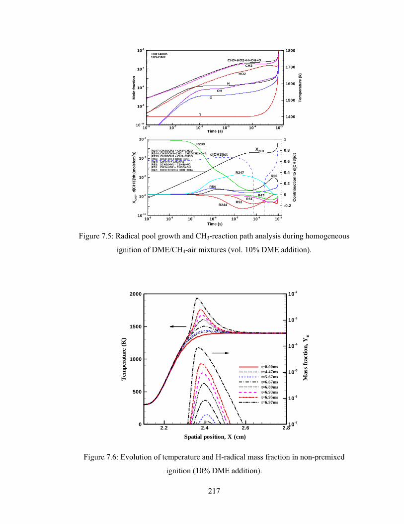
Time (s)
Tem
pera
ture
(k)
Mol
efra
ctio
n10-8 10-7 10-6 10-5 10-4 10-3
1400
1500
1600
1700
1800
10-10
10-8
10-6
10-4
10-2
T
O
OH
H
HO2
CH3CH3+HO2+H+OH+O
T0=1400K10%DME
Time (s)
XC
H3,
d[C
H3]
/dt(
mol
e/cm
3 s)
Con
tribu
ctio
nto
d[C
H3]
/dt
10-9 10-8 10-7 10-6 10-5 10-4 10-310-10
10-8
10-6
10-4
10-2
-0.2
0
0.2
0.4
0.6
0.8
1
d[CH3]/dt
R247
R239XCH3
R51
R244R52
R56
R54
R47
R247: CH3OCH2 = CH3+CH2OR244: CH3OCH3+CH3 = CH3OCH2+CH4R239: CH3OCH3 = CH3+CH3OR56: CH4+OH = CH3+H2OR54: CH4+H = CH3+H2R52: 2CH3(+M) = C2H6(+M)R51: CH3+HO2 = CH3O+OHR47: CH3+CH2O = HCO+CH4
Figure 7.5: Radical pool growth and CH3-reaction path analysis during homogeneous
ignition of DME/CH4-air mixtures (vol. 10% DME addition).
Mas
sfr
actio
n,Y
H
10-7
10-6
10-5
10-4
10-3
10-2
t=0.00mst=4.47mst=5.67mst=6.67mst=6.89mst=6.93mst=6.95mst=6.97ms
Spatial position, X (cm)
Tem
pera
ture
(K)
2.2 2.4 2.6 2.80
500
1000
1500
2000
Figure 7.6: Evolution of temperature and H-radical mass fraction in non-premixed
ignition (10% DME addition).
217

0 20 40 60 80 10-4
-3
-2
-1
0
Homogeneous Ignition
Nonpremixed Ignition a=300 s-1
a=200 s-1
a=100 s-1 a=20 s-1
Log
(igni
tion
dela
y (s
))
Volume percentage of DME in DME+CH4
Figure 7.7: Effects of DME addition on ignition delay of methane at atmospheric
pressure.
10-5 10-4 10-3 10-20.0
1.0x10⁻⁵
2.0x10⁻⁵
3.0x10⁻⁵
4.0x10⁻⁵
5.0x10⁻⁵
6.0x10⁻⁵
7.0x10⁻⁵
2% DME
200s-1
10% DME
a=20s-1
Max
imum
mas
s fr
actio
n of
CH
3
Time (s)
200s-1
20s-1
Figure 7.8: Evolution of the maximum mass fraction of CH3 in non-premixed ignition at
different stretch rates and DME addition levels.
218

0 20 40 60 80 10010
20
30
40
50
60
φ = 0.7
φ = 0.8
φ = 1.0
Flam
e sp
eed,
Su
(cm
/s)
Volume percentage of DME in DME+CH4
Symbols: experimentLines: prediction
Figure 7.9: Variation of laminar flame speeds of DME/CH4-air mixtures at different
equivalence ratios and DME blending at 298K, atmospheric pressure.
Volume percentage of DME in (DME+CH4)
Bur
ned
Mar
kste
inLe
ngth
,Lb
(mm
)
0 20 40 60 800.4
0.6
0.8
1
1.2
1.4
1 atm
ϕ = 0.8
100
ϕ = 1.0
ϕ = 1.2
Figure 7.10: Burned Markstein lengths of DME/CH4-air mixtures at different equivalence
ratios and DME blending at atmospheric pressure.
219
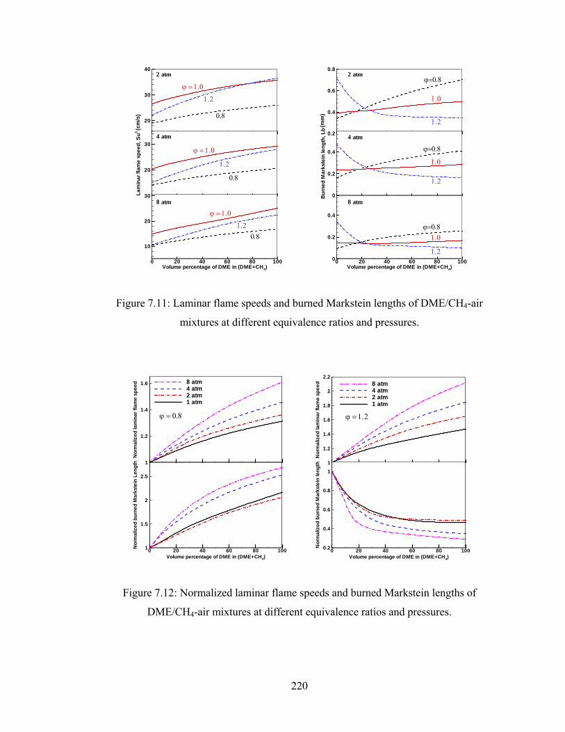
20
30
402 atm
0.2
0.4
0.6
0.82 atm
1.2
ϕ=0.8
(mm
)
ϕ = 1.0
1.01.2
0.8
(cm
/s)
Lam
inar
flam
esp
eed,
Su0
20
304 atm
1.2
0.8
ϕ = 1.0
Volume percentage of DME in (DME+CH4)0 20 40 60 80 100
10
20
308 atm
1.20.8
ϕ = 1.0
Volume percentage of DME in (DME+CH4)0 20 40 60 80 10
0.2
0.4
8 atm
00
1.2
ϕ=0.81.0
Bur
ned
Mar
kste
inle
ngth
,Lb
0
0.2
0.4
4 atm
1.2
ϕ=0.8
1.0
Figure 7.11: Laminar flame speeds and burned Markstein lengths of DME/CH4-air
mixtures at different equivalence ratios and pressures.
Volume percentage of DME in (DME+CH4)
Nor
mal
ized
burn
edM
arks
tein
Leng
th
0 20 40 60 80 11
1.5
2
2.5
00
Nor
mal
ized
lam
inar
flam
esp
eed
1
1.2
1.4
1.6 8 atm4 atm2 atm1 atm
ϕ = 0.8
Nor
mal
ized
lam
inar
flam
esp
eed
1
1.2
1.4
1.6
1.8
2
2.28 atm4 atm2 atm1 atm
ϕ = 1.2
Volume percentage of DME in (DME+CH4)
Nor
mal
ized
burn
edM
arks
tein
leng
th
0 20 40 60 80 10.2
0.4
0.6
0.8
1
00
Figure 7.12: Normalized laminar flame speeds and burned Markstein lengths of
DME/CH4-air mixtures at different equivalence ratios and pressures.
220
Chapter 8: Summary and Recommendations
8.1 Summary
In this dissertation, initiation, propagation, and extinction of premixed flames are
systematically investigated using asymptotic theoretical analysis, detailed numerical
simulations, and/or experimental measurements.
Specifically, in Chapter 2, a general theory to describe different flame regimes
and transitions among the flame kernel, the flame ball, the self-extinguishing flame, the
outwardly propagating spherical flame, and the propagating planar flame is obtained.
Based on this general theory, the dynamics of flame kernel evolution with and without
ignition energy deposition is studied and the effects of radiative heat loss and Lewis
number on flame propagation are investigated. It is found that the radiative heat loss from
the unburned and burned zones play different roles in affecting the flame propagation
speed. With the increase of flame radius, the radiative heat loss from the burned zone
increases, while that from the unburned zone decreases. As a result, there is a peak
radiation loss at an intermediate flame radius, which dramatically affects the flame
regimes. It is also found that the radiative heat loss from the unburned zone results in a
new flame regime: the isolated self-extinguishing flame with two radiation extinction
limits at small and large flame radii, respectively. In addition, radiative loss is found to
significantly affect the transition history of flame initiation when an external energy is
deposited.
In Chapter 3, a time-accurate and space-adaptive numerical solver for Adaptive
Simulation of Unsteady Reactive Flow (A-SURF) has been developed. It is shown that
221
A-SURF can accurately and efficiently simulate one-dimensional propagating flames
with detailed chemical mechanisms. A-SURF is currently the only numerical solver
which simulates propagating flames based on the compressible governing equations (thus
resolving acoustics) using detailed chemical mechanisms and adaptive meshes.
In Chapter 4, the controlling factor for spherical flame initiation and how it relates
to the minimum ignition energy are investigated by asymptotic analysis and detailed
numerical simulations. The results show that it is the critical flame radius, rather than the
flame thickness or flame ball radius, that controls the spherical flame initiation. The
minimum ignition energy for successful spherical flame initiation is found to be
proportional to the cube of the critical flame radius. Furthermore, preferential diffusion
between heat and mass (Lewis number effect) is found to play an important role in the
spherical flame initiation and it strongly affects the flame kernel evolution after ignition.
It is shown that both the critical flame radius and the minimum ignition energy increase
significantly with the Lewis number. Therefore, for transportation fuels with large Lewis
numbers, blending of small molecule fuels will significantly reduces ignition energy.
In Chapter 5, the constant pressure and constant volume methods utilizing
propagating spherical flames for laminar flame speed measurements are studied
theoretically and numerically. For the constant pressure method, the validity of the linear
relationship between flame speed and stretch and the effects of ignition, unsteady flame
transition, and compression on the accuracy of flame speed determination are
investigated. Theoretical analysis reveals a critical flame radius; only above which is the
linear or non-linear extrapolation for flame speeds valid. It is found that the critical radius
changes non-monotonically with the Lewis number and that, at large Lewis numbers, it
222

can be larger than the minimum flame radius used in experiments, leading to invalid
flame speed extrapolation. Besides, the ignition energy is shown to have a significant
impact on flame trajectories. It is found that the unsteady flame transition at different
ignition energies causes a flame speed reversal phenomenon that greatly narrows the
experimental data range for flame speed extrapolation. Furthermore, the compression
induced flow is shown to greatly affect both the instantaneous stretched and extrapolated
unstretched flame speeds. A Compression-Corrected Flame Speed (CCFS) method for
flame speed measurement is proposed to include the compression effect. It is
demonstrated that the present CCFS method not only increases the accuracy of the
measured flame speed but also extends the parameter range of experimental conditions.
For the constant volume method, the stretch effect is studied and an analytical expression
is derived to evaluate the stretch effect on the determination of laminar flame speeds. It is
shown that the stretch effect is proportional to the Markstein length and inversely
proportional to the flame radius. A Stretch-Corrected Flame Speed (SCFS) model is then
proposed to obtain accurate flame speed directly from the experimental measurements.
In Chapter 6, the effect of radiation on flame propagation and extinction is
investigated. In the first part, the outwardly and inwardly propagating flames (OPF and
IPF) are studied with the emphasis on the effects of radiative loss and preferential
diffusion on the flame propagation speed, Markstein number, and flame extinction.
Opposite trends for the change of the flame propagation speed and flame
extinction/flammability limits are found for the OPF and IPF at different Lewis numbers
and a correlation for Markstein length at different Lewis numbers and radiative losses is
obtained. In the second part, the spectrally dependent radiation absorption effect on flame
223
speed enhancement is measured by using CO2-diluted CH4/O2 mixtures at normal and
elevated pressures. The radiation absorption is found to increase the flame speed and to
extend the flammability limit. It is also shown that the spectrally dependent radiation
absorption needs to be included for quantitative predictions of flame speed and
flammability limit with CO2 addition: the FSNB-CK radiation model can well reproduce
the measured flame speed, while the SNB narrow-band gray model over-predicts the
flame speed and the optically thin model significantly under-predicts the flame speed. In
the third part, the flame dynamics of near limit premixed tubular flames are investigated
to reveal the combined effects of flame curvature, radiation, and stretch on flame
extinction. The coupling between radiation and flame curvature is found to lead to
multiple flame bifurcations and extinction limits for different radiation intensities. It is
also shown that both the stretch and radiation extinction limits are strongly affected by
flame curvature: the stretch extinction limit monotonically decreases with the increase of
flame curvature; while the radiation extinction limit, depending on the Lewis number,
either monotonically or non-monotonically changes with flame curvature.
In Chapter 7, the effects of DME addition to methane/air mixtures on the ignition,
flame speeds, and Markstein lengths are studied experimentally and computationally. In
homogeneous ignition, small amounts of DME addition to methane are found to
significantly decrease the ignition time. This significant ignition enhancement is caused
by the rapid build-up of CH3 and HO2 radicals when a small amount of DME is added to
the system. In non-homogeneous ignition, it is found that the ignition enhancement is
strongly affected by the stretch rate and there exist two ignition regimes: a kinetic limited
regime and a transport limited regime. In contrast to the nonlinear behaviour appeared in
224

ignition enhancement, the flame speeds of DME/CH4-air mixture are found to be linearly
proportional to the DME fraction. Moreover, it is found that the enhancement of the
flame speed by DME addition becomes stronger at higher pressures. Unlike the laminar
flame speeds, the Markstein lengths of the dual fuel change dramatically at small DME
concentrations and have different trends: increase at fuel lean (φ=0.8), decrease at fuel
rich (φ=1.2), and little increase at stoichiometric (φ=1.0). These changes are also found to
be significantly affected by the pressure.
8.2 Recommendations for Future Work
Based on the results of the present study, the following are some
recommendations for potential improvements on our understanding of premixed flame
initiation, propagation, and extinction.
For ignition, our theoretical and numerical analyses show that there exists a
critical flame radius controlling the spherical flame initiation and that the minimum
ignition energy is proportional to the cube of the critical flame radius. However, very few
experiments have been conducted to study the critical flame radius and its relationship to
the minimum ignition energy. Recent experiments by Kelly et al. (Kelley et al. 2008) on
hydrogen/air ignition at different equivalence ratios and pressures confirmed that there
was a critical flame radius for spherical flame initiation and successful ignition depended
on whether the initially ignited flame kernel could attain this critical radius. However, the
minimum ignition energy was not measured and thus its relationship with the critical
flame radius was not examined. Similar to the detailed numerical simulations shown in
Chapter 4, ignition experiments on different H2/O2/He/Ar and CH4/O2/He/Ar mixtures
are currently on our laboratory’s schedule. By changing the helium and argon fractions
225

while fixing their combined volume, the preferential diffusion effect as well as the
correlation between the critical flame radius and the minimum ignition energy will be
revealed. Moreover, it is of practical interest to study the ignition of fuel mixtures since
different fuel blends could be utilized for ignition control. According to the present study,
both the critical flame radius and the minimum ignition energy increase significantly with
the Lewis number. Therefore, for transportation fuels with large Lewis numbers, adding
small-molecule fuel will significantly reduces the ignition energy.
For flame propagation, either the constant pressure method or the constant volume
method was used in all the previous experiments. With the help of the
Compression-Corrected Flame Speed (CCFS) and the Stretch-Corrected Flame Speed
(SCFS) developed in Chapter 5, both methods could be utilized for the same run by
experiments conducted in a spherical chamber with windows for Schlieren imaging and
sensors for pressure recording (i.e. both the flame front and pressure histories could be
recorded). Using these methods, accurate flame speed data should be experimentally
determined at high pressures and high temperatures since many practical combustion
devices operate near these conditions. Moreover, compared with the laminar flame
speeds, the discrepancies among the Markstein lengths obtained from measurements are
much larger. Therefore, efforts need be spent on accurately measuring the Markstein
length using the constant pressure method. In addition, comparison between the constant
pressure method and the counterflow flame method needs to be conducted since different
laminar flame speeds and Markstein lengths are reported from experiments for the same
mixture at the same conditions.
226

For flame extinction, the combined effects of radiation, stretch, and curvature are
only investigated theoretically based on the premixed tubular flames. Experiments
utilizing a tubular burner should be conducted to validate the theoretical predictions.
Besides, numerical simulations of premixed tubular flames with detailed chemical
mechanisms will also help to understand these combined effects on flame extinction. In
addition, experiments on radiation absorption effect reported in Chapter 6 were
conducted at normal gravity. For near-limits flames, the laminar flame speeds are lower
than 10 cm/s and thus the buoyancy effect can not be neglected. Microgravity
experiments should be conducted to further understand the radiation absorption effect on
laminar flame speeds and flammability limits. These experiments will also help to reveal
the radiation effect on the accuracy of flame speed measurements using propagating
spherical flames. Furthermore, the correlation between the Markstein length and the
radiative heat loss derived in Chapter 6 could be checked by results from microgravity
experiments.
227

References
Addabbo, R., Bechtold, J.K. and Matalon, M. (2003). Proceedings of the Combustion Institute 29: 1527-1535.
Akram, M. (1996). AIAA Journal 34: 1835-1842.
Andrews, G.E. and Bradley, D. (1972). Combustion and Flame 18: 133-153.
Arcounianis, C., Bae, C., Crookes, R. and Kinoshita, E. (2008). Fuel 87: 1014-1030.
Aung, K.T., Hassan, M.I. and Faeth, G.M. (1997). Combustion and Flame 109: 1-24.
Bechtold, J.K., Cui, C. and Matalon, M. (2005). Proceedings of the Combustion Institute 30: 177-184.
Bechtold, J.K. and Matalon, M. (1987). Combustion and Flame 67: 77-90.
Bradley, D., Gaskell, P.H. and Gu, X.J. (1996). Combustion and Flame 104: 176-198.
Bradley, D., Hicks, R.A., Lawes, M., Sheppard, C.G.W. and Woolley, R. (1998). Combustion and Flame 115: 126-144.
Bradley, D., Lawes, M., Liu, K., Verhelst, S. and Woolley, R. (2007). Combustion and Flame 149: 162-172.
Bradley, D. and Mitcheson, A. (1976). Combustion and Flame 26: 201-217.
Brown, P.N., Byrne, G.D. and Hindmarsh, A.C. (1989). SIAM Journal on Scientific and Statistical Computing 10: 1038-1051.
Buckmaster, J.D. (1976). Combustion and Flame 26: 151-162.
Buckmaster, J.D. (1997). Combustion Theory and Modelling 1: 1-11.
Buckmaster, J.D., Joulin, G. and Ronney, P.D. (1990). Combustion and Flame 79: 381-392.
Buckmaster, J.D. (1982). Quarterly Journal of Mechanics and Applied Mathematics 35: 249-263.
Buckmaster, J.D., Joulin, G. and Ronney, P.D. (1991). Combustion and Flame 84: 411-422.
Buckmaster, J.D. and Lundford, G.S.S. (1982). Theory of laminar flames, Cambridge University Press.
Burke, M.P., Chen, Z., Ju, Y. and Dryer, F.L. (2009). Combustion and Flame, In press.
Champion, M., Deshaies, B., Joulin, G. and Kinoshita, K. (1986). Combustion and Flame 65: 319-337.
Chen, Z., Burke, M.P. and Ju, Y. (2008a). Proceedings of the Combustion Institute 32: Accepted.
Chen, Z., Burke, M.P. and Ju, Y. (2008b). AIAA 2008-0977.
228

Chen, Z., Burke, M.P. and Ju, Y. (2008c). SIAM: 12th International Conference on Numerical Combustion, Monterey, California, USA.
Chen, Z. and Ju, Y. (2007). Combustion Theory and Modelling 11: 427-453.
Chen, Z. and Ju, Y. (2008). International Journal of Heat and Mass Transfer 51: 6118-6125.
Chen, Z., Qin, M., Xu, B., Ju, Y.G. and Liu, F.S. (2007a). Proceedings of the Combustion Institute 31: 2693-2700.
Chen, Z., Qin, X. and Ju, Y. (2007b). 18th International Symposium on Transport Phenomena, Daejeon, Korea.
Chen, Z., Qin, X., Ju, Y.G., Zhao, Z.W., Chaos, M. and Dryer, F.L. (2007c). Proceedings of the Combustion Institute 31: 1215-1222.
Chung, S.H. and Law, C.K. (1988). Combustion and Flame 72: 325-336.
Clavin, P. (1985). Progress in Energy and Combustion Science 11: 1-59.
Clavin, P. (1994). Annual Review of Fluid Mechanics 26: 321-352.
Clavin, P. and Williams, F.A. (1982). Journal of Fluid Mechanics 116: 251-282.
Curran, H.J. (2005). Private Communication.
Curran, H.J., Fischer, S.L. and Dryer, F.L. (2000). International Journal of Chemical Kinetics 32: 741-759.
Curran, H.J., Pitz, W.J., Westbrook, C.K., Dagaut, P., Boettner, J.C. and Cathonnet, M. (1998). International Journal of Chemical Kinetics 30: 229-241.
Darrieus, G. (1938). Communication presented at La Technique Moderne.
Deshaies, B. and Joulin, G. (1984). Combustion Science and Technology 37: 99-116.
Dowdy, D.R., Smith, D.B., Taylor, S.C. and Williams, A. (1990). Proceedings of the Combustion Institute 23: 325-332.
Egolfopoulos, F.N., Cho, P. and Law, C.K. (1989). Combustion and Flame 76: 375-391.
Ekici, O., Ezekoye, O.A., Hall, M.J. and Matthews, R.D. (2007). Journal of Fluids Engineering-Transactions of the Asme 129: 55-65.
Farrell, J.T., Johnston, R.J. and Androulakis, I.P. (2004). Molecular structure effects on laminar burning velocities at elevated temperature and pressure. SAE paper, 2004-01-2936.
Fischer, S.L., Dryer, F.L. and Curran, H.J. (2000). International Journal of Chemical Kinetics 32: 713-740.
Flaherty, J.E., Frankel, M.L., Roytburd, V. and Sivashinsky, G.I. (1985). Combustion Science and Technology 43: 245-257.
Frank-Kamenetskii, D. (1955). Diffusion and heat exchange in chemical kinetics, Princeton University Press, Princeton.
229
Frankel, M.L. and Sivashinsky, G.I. (1983). Combustion Science and Technology 31: 131-138.
Frankel, M.L. and Sivashinsky, G.I. (1984). Combustion Science and Technology 40: 257-268.
Frendi, A. and Sibulkin, M. (1990). Combustion Science and Technology 73: 395-413.
Glassman, I. (1996). Combustion, 3rd edition. Academic Press.
Gottlieb, S. and Shu, C.W. (1998). Mathematics of Computation 67: 73-85.
Groot, G.R.A., van Oijen, J.A., de Goey, L.P.H., Seshadri, K. and Peters, N. (2002). Combustion Theory and Modelling 6: 675-695.
Gu, X.J., Haq, M.Z., Lawes, M. and Woolley, R. (2000). Combustion and Flame 121: 41-58.
Guo, H., Ju, Y., Maruta, K., Niioka, T. and Liu, F. (1998). Combustion Science and Technology 135: 49-64.
Hassan, M.I., Aung, K.T. and Faeth, G.M. (1998). Combustion and Flame 115: 539-550.
He, L. and Law, C.K. (1999). On the dynamics of transition from propagating flame to stationary flame ball, AIAA 99–0325.
He, L. (2000). Combustion Theory and Modelling 4: 159-172.
Hill, P.G. and Hung, J. (1988). Combustion Science and Technology 60: 7-30.
Hinshelwood, C.N. (1940). The kinetics of chemical changes, Oxford University Press, London.
Huang, Y., Sung, C.J. and Eng, J.A. (2004). Combustion and Flame 139: 239-251.
Huzayyin, A.S., Moneib, H.A., Shehatta, M.S. and Attia, A.M.A. (2008). Fuel 87: 39-57.
Ishizuka, S. (1993). Progress in Energy and Combustion Science 19: 187-226.
Jomaas, G. (2008). Propagation and stability of expanding spherical flames, Princeton University. Ph.D. Thesis.
Joulin, G. (1985). Combustion Science and Technology 43: 99-113. Joulin, G. and Clavin, P. (1979). Combustion and Flame 35: 139-153.
Joulin, G. and Deshaies, B. (1986). Combustion Science and Technology 47: 299-315.
Joulin, G. and Mitani, T. (1981). Combustion and Flame 40: 235-246.
Ju, Y., Maruta, K. and Niioka, T. (2001). Applied Mechanical Review 54: 257-277.
Ju, Y., Masuya, G., Liu, F., Hattori, Y. and Riechelmann, D. (2000). International Journal of Heat and Mass Transfer 43: 231-239.
Ju, Y., Masuya, G. and Ronney, P.D. (1998). Proceedings of the Combustion Institute 27: 2619-2626.
Ju, Y.G., Guo, H.S., Liu, F.S. and Maruta, K. (1999a). Journal of Fluid Mechanics 379: 165-190.
230

Ju, Y.G., Guo, H.S., Maruta, K. and Liu, F.S. (1997). Journal of Fluid Mechanics 342: 315-334.
Ju, Y.G., Matsumi, H., Takita, K. and Masuya, G. (1999b). Combustion and Flame 116: 580-592.
Karlovitz, B., Denniston Jr., D.W., Knapschaefer, D.H. and Wells, F.E. (1953). Proceedings of the Combustion Institute 4: 613-620.
Kee, R.J., Grcar, J.F., Smooke, M.D. and Miller, J.A. (1985). A FORTRAN program for modeling steady laminar one-dimensional premixed flames, Sandia National Laboratory Report SAND85-8240.
Kee, R.J., Rupley, F.M. and Miller, J.A. (1989). CHEMKIN-II: A FORTRAN package for the analysis of gas-phase chemical kinetics, Sandia National Laboratory Report SAND89-8009B.
Kelley, A.P., Jomaas, G. and Law, C.K. (2008). AIAA 2008-1054.
Kelly, A.P. and Law, C.K. (2007). Fall technical meeting: Eastern states sections of the combustion institute, Virginia, Paper B-11.
Kim, T.K., Menart, J.A. and Lee, H.S. (1991). Journal of Heat Transfer-Transactions of the Asme 113: 946-952.
Kobayashi, H. and Kitano, M. (1989). Combustion and Flame 76: 285-295.
Kobayashi, H. and Kitano, M. (1993). Combustion Science and Technology 89: 253-263.
Kwon, S., Tseng, L.K. and Faeth, G.M. (1992). Combustion and Flame 90: 230-246.
Landau, L. (1944). Acta Physicochimica Urss 19: 77-85.
Law, C.K. (2006). Combustion physics, Cambridge University Press.
Law, C.K., Sung, C.J., Wang, H. and Lu, T.F. (2003). AIAA Journal 41: 1629-1646.
Levy, A. and Weinberg, F.J. (1959). Proceedings of the Combustion Institute 7: 296-303.
Lewis, B. and Von Elbe, G. (1961). Combustion flames and explosive of gases, Academic Press, New York. Li, J., Zhao, Z.W., Kazakov, A. and Dryer, F.L. (2004). International Journal of Chemical Kinetics 36: 566-575.
Liu, F., Gulder, O.L., Smallwood, G.J. and Ju, Y. (1998). International Journal of Heat and Mass Transfer 41: 2227-2236.
Lozinski, D., Buckmaster, J. and Ronney, P. (1994). Combustion and Flame 97: 301-316.
Lutz, A.E., Kee, R.J. and Miller, J.A. (1987). SENKIN: A FORTRAN program for predicting homogeneous gas phase chemical kinetics with sensivity analysis, Sandia National Laboratory Report SAND87-8248.
Maas, U. and Warnatz, J. (1988). Combustion and Flame 74: 53-69.
Markstein, G.H. (1951). Journal of the Aeronautical Sciences 18: 199-209.
Markstein, G.H. (1964). Nonsteady flame propagation, Pergamon Press.
231

Maruta, K., Yoshida, M., Ju, Y. and Niioka, T. (1996). Proceedings of the Combustion Institute 26: 1283-1289.
Matalon, M. (1983). Combustion Science and Technology 31: 169-181.
Matthews, M.T., Dlugogorski, B.Z. and Kennedy, E.M. (2006). Combustion and Flame 144: 838-849.
Metghalchi, M. and Keck, J.C. (1980). Combustion and Flame 38: 143-154.
Mitani, T. (1980). Combustion Science and Technology 23: 93-101.
Mosbacher, D.M., Wehrmeyer, J.A., Pitz, R.W., Sung, C.J. and Byrd, J.L. (2003). Proceedings of the Combustion Institute 29: 1479-1486.
Müller, S. (2000). Adaptive multiscale schemes for conservation laws, Springer.
Nishioka, M., Inagaki, K., Ishizuka, S. and Takeno, T. (1991). Combustion and Flame 86: 90-100.
Nishioka, M., Takeno, T. and Ishizuka, S. (1988). Combustion and Flame 73: 287-301.
Parsinejad, F., Arcari, C. and Metghalchi, H. (2006). Combustion Science and Technology 178: 975-1000.
Peters, N. (2000). Turbulent combustion. New York, Cambridge University Press.
Piessens, R., Doncker-Kapenger, E., Ueberhuber, C. and Kahaner, D. (1983). QUADPACK, a subroutine package for automatic integration, Springer Verlag.
Poinsot, T. and Veynante, D. (2005). Theoretical and numerical combustion, R.T. Edwards, Inc.
Qin, X. and Ju, Y.G. (2005). Proceedings of the Combustion Institute 30: 233-240.
Rallis, C.J. and Garforth, A.M. (1980). Progress in Energy and Combustion Science 6: 303-329.
Ronney, P.D. (1985). Combustion and Flame 62: 121-133.
Ronney, P.D. (1988). Proceedings of the Combustion Institute 22: 1615-1623.
Ronney, P.D. (1990). Combustion and Flame 82: 1-14. Ronney, P.D. (1994). Optical Engineering 33: 510-521.
Ronney, P.D. and Sivashinsky, G.I. (1989). SIAM Journal on Applied Mathematics 49: 1029-1046.
Ronney, P.D. and Wachman, H.Y. (1985). Combustion and Flame 62: 107-119.
Rozenchan, G., Zhu, D.L., Law, C.K. and Tse, S.D. (2003). Proceedings of the Combustion Institute 29: 1461-1470.
Ruan, J.M., Kobayashi, H., Niioka, T. and Ju, Y.G. (2001). Combustion and Flame 124: 225-230.
Saeed, K. and Stone, C.R. (2004). Combustion and Flame 139: 152-166.
232

Semelsberger, T.A., Borup, R.L. and Greene, H.L. (2006). Journal of Power Sources 156: 497-511.
Semenov, N.N. (1935). Chemical kinetics and chain reactions, Oxford University Press, London.
Sivashinsky, G.I. (1977). Combustion Science and Technology 15: 137-146.
Sloane, T.M. and Ronney, P.D. (1993). Combustion Science and Technology 88: 1-13.
Smith, G.P., Golden, D.M., Frenklach, M., Moriarty, N.W., Eiteneer, B., Goldenberg, M., Bowman, C.T., Hanson, R.K., Song, S., Gardiner, W.C., Jr., Lissianski, V.V. and Qin, Z., http://www.me.berkeley.edu/gri_mech/.
Sod, G.A. (1978). Journal of Computational Physics 27: 1-31.
Sohrab, S.H. and Law, C.K. (1984). International Journal of Heat and Mass Transfer 27: 291-300.
Spalding, D.B. (1957). Proceedings of the Royal Society of London Series a-Mathematical and Physical Sciences 240: 83-100.
Strang, G. (1968). SIAM Journal on Numerical Analysis 5: 506-517.
Sun, C.J. and Law, C.K. (1998). Proceedings of the Combustion Institute 27: 963-970.
Sun, C.J., Sung, C.J., He, L. and Law, C.K. (1999). Combustion and Flame 118: 108-128.
Sun, M. (1998). Numerical and experimental studies of shock wave interaction with bodies, Tohoku University. Ph.D. Thesis.
Sun, M. and Takayama, K. (1999). Journal of Computational Physics 150: 143-180.
Sung, C.J. and Law, C.K. (1996). Proceedings of the Combustion Institute 26: 865-873.
Takeno, T. and Ishizuka, S. (1986). Combustion and Flame 64: 83-98.
Takeno, T., Nishioka, M. and Ishizuka, S. (1986). Combustion and Flame 66: 271-283.
Takizawa, K., Takahashi, A., Tokuhashi, K., Kondo, S. and Sekiya, A. (2005). Combustion and Flame 141: 298-307. Taylor, S.C. (1991). Burning velocity and the influence of flame stretch, University of Leeds. Ph.D. Thesis.
Thiele, M., Selle, S., Riedel, U., Warnatz, J. and Maas, U. (2000). Proceedings of the Combustion Institute 28: 1177-1185.
Thiele, M., Warnatz, J., Dreizler, A., Lindenmaier, S., Schiessl, R., Maas, U., Grant, A. and Ewart, P. (2002). Combustion and Flame 128: 74-87.
Toro, E.F. (1999). Riemann solvers and numerical methods for fluid dynamics, Springer.
Tromans, P.S. and Furzeland, R.M. (1988). Proceedings of the Combustion Institute 21: 1891-1897.
Tse, S.D., Zhu, D.L. and Law, C.K. (2000). Proceedings of the Combustion Institute 28: 1793-1800.
233

Tseng, L.K., Ismail, M.A. and Faeth, G.M. (1993). Combustion and Flame 95: 410-426.
Tsuji, H. (1982). Progress in Energy and Combustion Science 8: 93-119.
van Leer, B. (1984). SIAM Journal on Scientific and Statistical Computing 5: 1-20.
Van maaren, A., Thung, D.S. and Degoey, L.P.H. (1994). Combustion Science and Technology 96: 327-344.
Vazquez-Espi, C. and Linan, A. (2001). Combustion Theory and Modelling 5: 485-498.
Vazquez-Espi, C. and Linan, A. (2002). Combustion Theory and Modelling 6: 297-315.
Wang, P., Wehrmeyer, J.A. and Pitz, R.W. (2006). Combustion and Flame 145: 401-414.
Williams, F.A., http://maeweb.ucsd.edu/~combustion/.
Williams, F.A. (1985). Combustion theory, Benjamin-Cummins, Menlo Park, CA.
Wu, M.S., Ronney, P.D., Colantonio, R.O. and Vanzandt, D.M. (1999). Combustion and Flame 116: 387-397.
Yao, M., Qin, J. and Zheng, Z. (2005). Proceedings of the Institution of Mechanical Engineers Part D-Journal of Automobile Engineering 219: 1225-1236.
Yokomori, Y., Chen, Z. and Ju, Y. (2006). AIAA 2006-0161.
Zeldovich, Y.B., Barenblatt, G.I., Librovich, V.B. and Makhviladze, G.M. (1985). The mathematical theory of combustion and explosions, New York: Consultants Bureau.
Zhao, Z., Chaos, M., Kazakov, A. and Dryer, F.L. (2008). International Journal of Chemical Kinetics 40: 1-18.
Zheng, X.L., Lu, T.F., Law, C.K., Westbrook, C.K. and Curran, H.J. (2005). Proceedings of the Combustion Institute 30: 1101-1109.
234