subjective survival probabilities in the health and - deep blue

Working Paper

WP 2007-159

Project #: UM07-19 M RR C

Subjective Survival Probabilities in the Health and Retirement Study: Systematic Biases and Predictive Validity

Todd E. Elder

MichiganUniversity of

Research

Retirement

Center


Todd E. Elder Michigan State University

October 2007

Michigan Retirement Research Center University of Michigan

P.O. Box 1248 Ann Arbor, MI 48104

http://www.mrrc.isr.umich.edu/ (734) 615-0422

Acknowledgements This work was supported by a grant from the Social Security Administration through the Michigan Retirement Research Center (Grant # 10-P-98362-5-04). The findings and conclusions expressed are solely those of the author and do not represent the views of the Social Security Administration, any agency of the Federal government, or the Michigan Retirement Research Center. Regents of the University of Michigan Julia Donovan Darrow, Ann Arbor; Laurence B. Deitch, Bingham Farms; Olivia P. Maynard, Goodrich; Rebecca McGowan, Ann Arbor; Andrea Fischer Newman, Ann Arbor; Andrew C. Richner, Grosse Pointe Park; S. Martin Taylor, Gross Pointe Farms; Katherine E. White, Ann Arbor; Mary Sue Coleman, ex officio


Todd E. Elder

Abstract

Recent research has demonstrated that retirement planning and well-being are closely tied to probabilistic forecasts about future events. Using longitudinal data from the Health and Retirement Study, I show that individuals’ subjective survival forecasts exhibit systematic biases relative to life table data. In particular, many respondents fail to account for increases in yearly mortality rates with age, both longitudinally and in cross-section. Additionally, successive cohorts of the near elderly do not appear to revise survival forecasts to match increases in longevity. Forecasting bias may merely be due to the framing of questions designed to elicit expectations, but real biases may result in suboptimal savings rates and timing of retirement. Cross-sectional variation in subjective survival forecasts also appears to reflect differences in cognitive ability across respondents, suggesting that subjective information is more relevant for some individuals than others. Despite these shortcomings, subjective mortality probabilities predict actual mortality and portfolio choice, and they contain information not found in selfreported health status or objective measures of health limitations.

Authors’ Acknowledgements

I thank seminar participants at Michigan State University and the Michigan Retirement Research Center’s annual workshop for helpful comments and suggestions. I am especially grateful for the financial support provided by the U.S. Social Security Administration through the Michigan Retirement Research Center, funded as part of the Retirement Research Consortium (Project ID #UM07-19). The opinions and conclusions expressed are solely those of the author and should not be construed as representing the opinions or policy of SSA or any agency of the Federal Government. Email: [email protected].

3

I. Introduction

The life-cycle model highlights the central role of expectations about future events in

shaping the decisions of economic agents. Individuals acquire human capital and make decisions

about labor supply, consumption, and savings with the future in mind. In particular, subjective

expectations play a central role in retirement planning and well-being, and longevity risk

highlights the importance of the availability of annuities such as Social Security benefits relative

to relatively risky defined contribution or personal retirement accounts. Expectations about

future mortality also guide the decisions of firms and governments in the design of pensions and

old-age assistance programs. In spite of the widespread importance of expectations (particularly

mortality forecasts) in decision-making, economists have not had access to reliable data on

individual survival expectations until recently. As an alternative, researchers have typically

modeled economic behavior as a function of population-wide survival probabilities, as measured

by published life tables.

This study aims to investigate the validity and utility of relatively new sources of data on

individual subjective expectations about mortality. The Health and Retirement Study (HRS) and

the Asset and Health Dynamics Study (AHEAD) include numerous questions about expectations,

including the probability of working past ages 62 and 65, the probability of suffering a job loss in

the next year, and the probability of surviving to a selection of target ages. We analyze the

subjective assessments of the likelihood of surviving to a range of target ages, with a focus on

the evolution of these expectations over the life cycle in response to new information about one’s

health and the health and mortality of relatives and peers. The goal of this research is to shed

new light on longstanding questions about the effects of information and financial planning

education on the adequacy of retirement savings among the elderly. In particular, do subjective

expectations (and deviations of these expectations from population-wide life tables) influence

4

retirement, initial claiming of Social Security, and saving and asset allocation decisions among

elderly individuals in the United States? If so, researchers could incorporate errors in conditional

survival forecasts into dynamic models of retirement and savings, highlighting the effects of

mortality uncertainty on possible failures to smooth consumption at the end of the life cycle.

Previous research on probabilistic expectations has attempted to assess the reliability of

these measures in a number of ways. Hurd and McGarry (1995) and Manski (2004) find

substantial correlations between expectations and characteristics that actually affect mortality,

such as tobacco use and regular physical activity. Hurd et al (1998) and Hurd and McGarry

(2002) find that survival self-assessments closely track future mortality in 6-year panels of the

HRS. Lillard and Willis (2001) and Kézdi and Willis (2003) take a novel approach, highlighting

the role of the precision of individuals’ subjective assessments (rather than just the assessments

themselves) on asset allocation and benefit claiming decisions.1 This project extends the previous

research by focusing on conditional mortality expectations and by investigating the role of

planning horizons and the framing of questions designed to elicit expectations as two possible

sources of expectation errors.

The following section describes the data used and provides an informal description of the

usefulness of subjective survival assessments. Section III focuses on conditional probabilities of

survival, including a test of the notion that individuals cannot accurately forecast increases in

yearly mortality rates with age. Section IV explores strategies for identifying whether subjective

assessments predict actual mortality and retirement. Section V presents evidence on the role of

new information and cognition in revisions of longevity expectations, with the results implying

that changes (specifically, declines) in health are largely unexpected, since survival expectations

1 Kézdi and Willis use a battery of the subjective questions administered in the HRS to construct an “index of

precision”, inversely related to the fraction of focal probability answers (answers of exactly 0, 50, or 100 percent).

5

generally rise with age only when health does not change. Section VI investigates the role of

subjective beliefs on economic outcomes, particularly asset allocation decisions, and Section VII

concludes.

II. Data and Measures of Survival Forecasts

The HRS is a national panel study that surveys four different cohorts. The original HRS

cohort, born between 1931 and 1941, was first interviewed in 1992 and subsequently every two

years. The AHEAD cohort, consisting of individuals born before 1924, was initially a separate

study from the HRS but has been part of the HRS since 1998. Third is the Children of

Depression (CODA) cohort, born between 1924 and 1930 and first interviewed in 1998, and

finally the War Baby (WB) cohort, born between 1942 and 1947 and also first interviewed in

1998. In the original HRS cohort, a cross-section representative of the non-institutionalized

population was selected for interview, as well as an oversample of African-Americans and

Hispanics. The HRS also interviewed spouses and domestic partners of target respondents,

resulting in 12,652 individuals included in Wave 1.

The first AHEAD interview, in 1993, represents the non-institutionalized population aged

70 and older. Respondents were reinterviewed in 1995 and then at two-year intervals starting in

1998. Also in 1998, these cohorts were combined with the CODA cohort, meant to fill in the 9-

year age window not covered by the original HRS or the AHEAD, and the WB, intended to

include those aged 51-56 in 1998. From 1998 forward, the complete HRS sampling frame is

meant to represent the population of Americans over age 50 who do not live in institutional

settings (such as nursing homes).2

2 This sampling design is intended to replicate the population represented by the Current Population Survey (CPS).

6

For this study, the primary measure of interest is derived from HRS respondents’ answers

to three questions of the form:

“On a scale from 0 to 100, where 0 is no chance and 100 is absolutely certain, what are

the chances that you will live to age X or older?”

All Wave 1 through 7 HRS/AHEAD respondents under age 65 were asked this question for X =

75, and all respondents in Waves 1 through 4 under age 85 in the HRS were asked this question

for X = 85. Denote the answers to these questions as P75 and P85. From Wave 5 onward and in

all AHEAD waves, the latter question was replaced with one that asked about the likelihood of

living roughly another 11 to 15 years. Specifically, those under age 70 were asked the likelihood

of surviving to age 80; those between the ages of 70 and 74 were asked the likelihood of

surviving to age 85; and so on

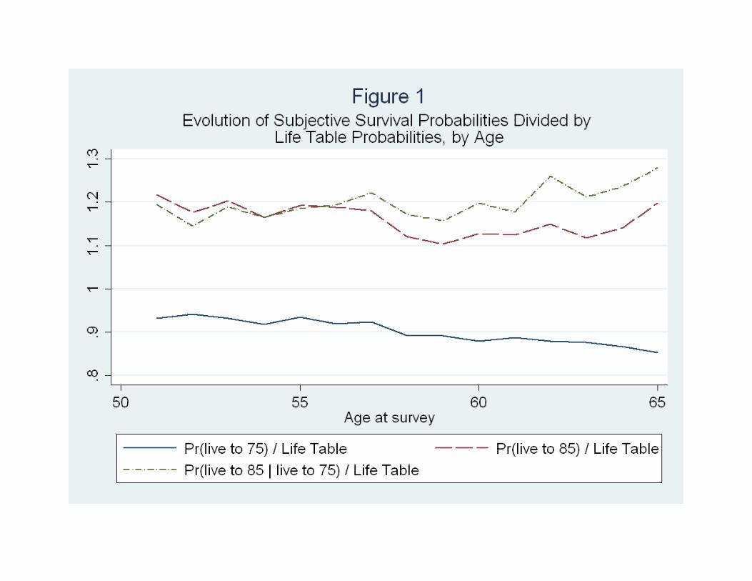
Figure 1 plots age-specific average responses of P75, P85, and P(live to 85 | live to 75),

which is calculated from the ratio of the likelihood of surviving to age 85 and the likelihood of

survival to age 75: P85 / P75, divided by the corresponding life table probabilities. The figure

shows that pessimism in P75 gradually increases with the age of the respondents (a ratio of 1

indicates an “accurate forecast” for a representative individual, relative to life tables). This

pattern is driven by the fact that, unlike life tables, average values of P75 do not increase with

age. Optimism in reports of both P85 and P85 / P75 appear roughly constant across age. The

pattern represented by Figure 1 does not vary with individual characteristics such as income,

education, or race; perhaps surprisingly, these crude proxies of cognitive ability or financial

planning literacy do little to explain the systematic positive bias in evaluations of subjective

mortality. On average, individuals at all ages slightly understate P75 and overstate P85 relative to

7

life table data, but both errors are subtle enough to lead previous researchers to assert that

expectations are accurate overall.

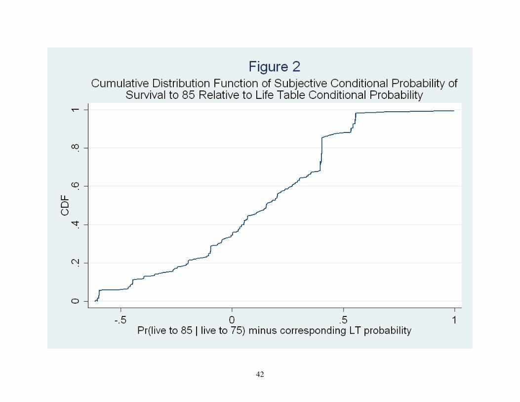
Figure 2 presents complementary evidence that a substantial number of individuals over-

predict the probability of surviving to age 85 conditional on reaching age 75. The line in the

figure plots the cumulative distribution function of P85 / P75 from subjective data minus P85 / P75

from Vital Statistics life tables, revealing a large, systematic positive bias in self-reports. In

particular, the median over-prediction (corresponding to the point at which the CDF = 0.5) is

roughly 0.17, a large bias relative to the actual conditional probability of survival of 0.38. The

25th

percentile of the difference is -0.10, while the 75th

percentile is roughly 0.42. Only 34

percent of HRS respondents report conditional survival probabilities less than or equal to the

corresponding life table figures, which can be seen by noting the CDF evaluated at “zero error”

in the figure. As was the case for Figure 1, this apparent over-prediction holds across gender,

racial, and educational categories, suggesting that regardless of socioeconomic status, changes in

health near the end of the life cycle are difficult to assess in a probabilistic fashion.3

The preceding findings do not suggest a cause for the differences in accuracy between P75

and P85, but Figure 1 provides evidence that differences in forecasting horizons are not driving

the results. Those in their early fifties are pessimistic, on average, regarding the probability of

surviving to age 75. In contrast, individuals in their early sixties have sizeable optimistic biases

about the probability of surviving to age 85. The sharply increasing yearly death rates in the 65-

85 age range provide an alternative explanation for this phenomenon.4 We turn next to an

3 Some care should be taken in interpreting these results. Lillard and Willis (2001) find that individuals are more

likely to provide focal responses to questions about expectations of events far in the future, suggesting that distant

future events are sufficiently difficult to forecast (or that the wording of the questions is sufficiently difficult to

understand) that subjective probability assessments may not provide reliable information.

4 For a representative man in 1992, the one-year mortality probability increases from less than two percent at age 65

to over twelve percent by age 85.

8

analysis of whether HRS respondents may fail to understand the concept of increasing yearly

mortality hazard rates.

III. Increasing Hazards and the Usefulness of Subjective Responses

The previous section presented preliminary evidence about one possible source of error in

individual survival forecasts: individuals’ implied subjective distributions of age of death are

substantially flatter than published life tables indicate. Table 1 presents parallel evidence,

reporting the average values of P75 and P85 in five age categories and separately by gender. For

all age and gender combinations, the average probability of surviving to age 75 is larger than that

of living to age 85. At a first glance, the subjective measures correlate well with the life table

figures, but for all groups, assessments of survival to age 85 are substantially more optimistic

than those based on age 75. As previous studies (e.g., Hurd and McGarry (1995) and Hurd et al

(1998)) have found, men are generally more optimistic than women, relative to life tables. For

instance, men and women aged 65 report nearly identical average rates of surviving to ages 75

and 85, in spite of life table evidence that women are roughly nine percentage points more likely

to live to 75 and sixteen percentage points more likely to live to age 85. Men are slightly

pessimistic about living to 75 and quite optimistic about living to 85, while women appear very

pessimistic about survival to 75 and relatively accurate about survival to 85. Similar to the

findings of Hurd and McGarry (2002), the age gradient in subjective probabilities is flatter than

the corresponding gradient for life-table probabilities, but this pattern appears to be driven

entirely by the responses of women, who report only slight increases in survival probabilities

with age.

9

Table 2 shows the distribution of subjective responses across gender and within age

categories. “Focal responses”, involving probabilities of 0, 0.5, or 1, represent roughly half of all

responses to the age 75 question. One interpretation of focal responses is that they do not

represent accurate probabilities, but are based instead on rules of thumb regarding distant events

that are difficult to forecast. In light of this interpretation, it is surprising that focal responses are

less prevalent in answers to questions about surviving to age 85 than age 75. Moreover, the

proportion of focal responses does not decline with age, which is contrary to the notion that long

planning horizons are responsible for these responses. We will return to the issue of whether

focal responses represent accurate probabilities below.

The overall picture of Tables 1 and 2 implies that subjective probability responses satisfy

at least the most basic logical requirement of probabilities: they decrease with the planning

horizon. However, the implied flatness of subjective survival forecasts represents a systematic

bias relative to life table data. Hamermesh’s (1985) groundbreaking study of subjective survival

forecasts suggests that this flatness may stem from individuals being able to extrapolate current

life tables into the future, so that optimism about survival to age 85 may be rational. If future

increases in longevity affect mortality hazards for ages between 75 and 85 more than ages below

75, then the lack of optimism for age 75 survival rates makes sense, but this conjecture cannot

explain why individuals would be pessimistic about age 75 survival. Additionally, changes in

yearly life tables over the past decade suggest that decreases in death rates have occurred at

relatively young ages as well as ages over 75.

The notion that many individuals do not understand the concept of increasing yearly death

rates provides an alternative hypothesis to explain the flat subjective longevity profile. Consider a

discrete-time model of conditional probabilities of survival, where at any age t, the probability of

10

dying before reaching age t+1 is given by λt . It follows that the probability of surviving to age t2

given that an individual survives until age t1 is given by:

∏−

=

−++

−=

−×−−−=

1

121

12

2

1

2111

)1(

)1()1)((1)(1(

)|Pr(

t

tj

j

tttt

tagetolivetagetolive

λ

λλλλ

If per-year death rates are constant at the rate λ, then the probability of surviving to age t2 conditional

on survival to t1 is simply

12)1(

)|Pr( 12

tt

tagetolivetagetolive

−−= λ

So, for example, the probability of living to 75 for a 65 year old (i.e., conditional on reaching age 65)

is

Pr(live to age 75 | live to age 65) = (1 – λ)10

,

and the probability of living to 85 for a 65 year old is

Pr(live to age 85 | live to age 65) = (1 – λ)20

,

implying that P85 = (P75) 2 among 65 year olds. More generally, under the constant hazards

assumption, )85(

75

)75(

85ii AgeAge

PP−− = , where Agei is the current age of respondent i (time subscripts are

suppressed throughout). This implies that i

i

i

i PAge

AgeP )(log

75

85)(log 7585

−

−= , so that a weak form of a

test of constant subjective hazard rates is a test of the coefficients from the following linear

regression:

i

j

iji PjAgeP )(log)(1)(log 75

75

50

85 ∑=

=+= βα

As an informal test of this hypothesis, consider the two subjective probabilities among

those aged exactly 65. As noted above, if individuals (incorrectly) predict constant yearly death

11

rates, the probability of surviving 20 additional years will be the square of the probability of

living 10 additional years, so that P85 = (P75) 2

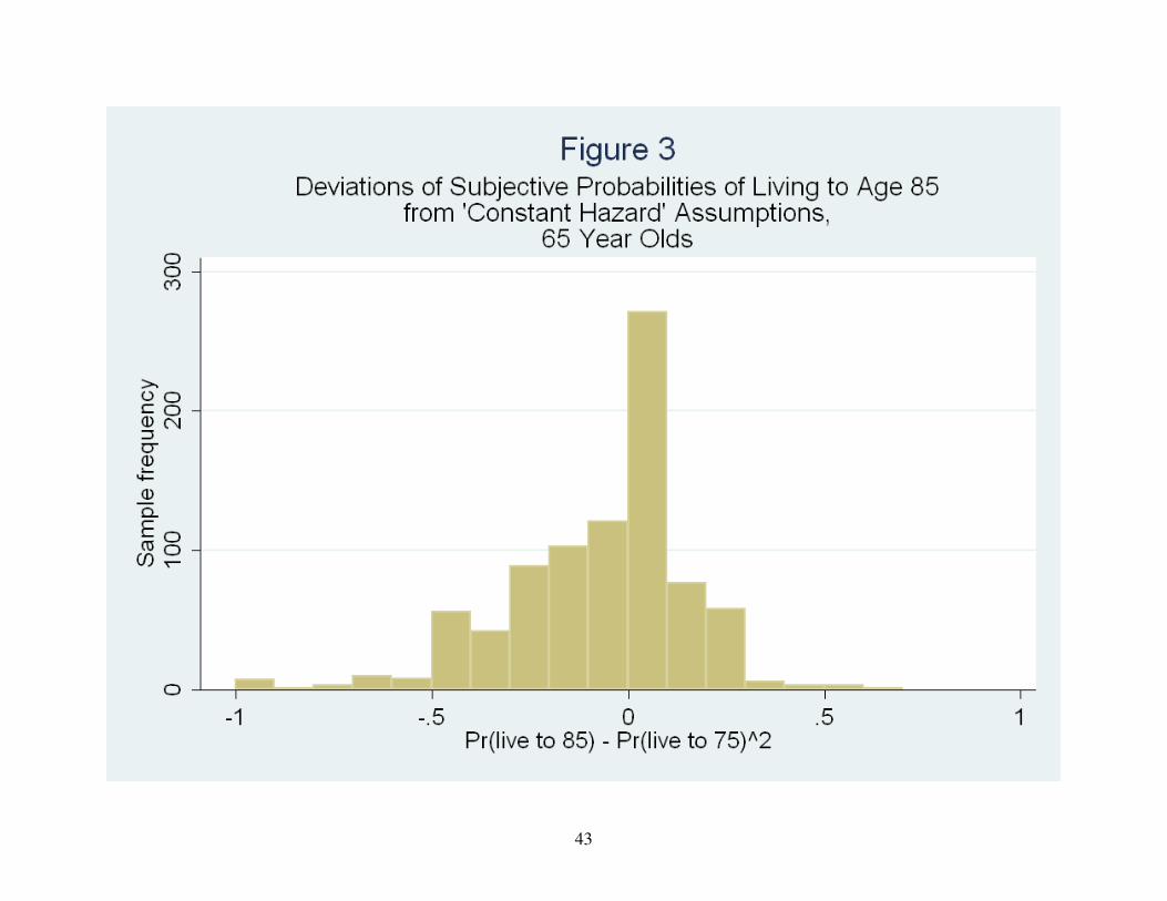
. Figure 3 presents the distribution of P85 - (P75)2

among 817 65 year-olds in the HRS who had valid responses to both subjective probability

questions. Nearly half of all respondents (46%) report P85 – (P75)2 ≥ 0, which would imply

weakly decreasing yearly death rates, and the mean value of P85 – (P75)2 is -0.04. Among this

age group, the hypothesis of constant subjective hazards appears to be reasonably accurate.5

Table 3 presents a more formal test of the constant hazard hypothesis based on linear

OLS and 2SLS models of the relationship between log(P85) and log(P75) for all individuals aged

50, 55, and 60 through 65 in the HRS. Column (1) shows estimates of βt from OLS regressions

with no additional covariates. A one-percent increase in P75 is associated with a 1.17 percent

increase in P85 among 50-year-old respondents. The associated standard error (in parentheses) is

0.04. The corresponding value implied by the constant hazard rate hypothesis is 1.40, and the

value from a similar regression that instead uses life table survival rates is 2.33. Note that the

value from the life table is substantially greater than that implied by the constant hazard

hypothesis because yearly mortality hazards increase sharply with age. In contrast, the fact that

the estimate in column (1) is below that in column (5) suggests that individuals’ subjective

forecasts imply decreasing yearly death rates with age. Also note that, in contrast to the values

in columns (4) and (5), the estimates in column (1) do not increase with age – the estimate for 65

year olds is 1.12 (0.04), roughly the same as that for 50 year olds.

The central obstacle in interpreting the estimates in column (1) of Table 3 is measurement

error in the values of log(P75) and log(P85). If measurement error in log(P75) is classical and

orthogonal to measurement error in values of log(P75) elicited in other time periods, then

5 The p-value for the hypothesis test is 0.18. The asymptotic distribution of the sample statistic is derived using

standard first-order Taylor Series expansions, and bootstrapped standard errors yield qualitatively similar results.

12

instrumental variables estimates using other time period values as instruments can deliver

consistent estimates of βt. Any lags or leads of log(P75) are possible candidate instruments;

column (2) of the table presents 2SLS estimates that instrument current log(P75) with the average

of all other values of log(P75) that the individual reported. All estimates from column (2) are

greater than the corresponding ones in column (1), but are smaller than those implied by constant

hazard rates for ages 60 and above. As in column (1), there does not appear to be an age gradient

in the estimated coefficients, which suggests that individuals do not update their subjective

probabilities as they age.

Column (3) of Table 3 presents 2SLS estimates using an additional identification

strategy. Previous authors such as Hamermesh (1985) and Hurd and McGarry (2002) have

found that respondents’ subjective survival rates are correlated with measures of their parents’

(and spouse’s) mortality experiences, but that these parental mortality measures are only weakly

correlated with self-reported health and more objective measures of health such as difficulties in

activities of daily living (ADL’s). These findings suggest another instrumental variables strategy

for testing the constant hazard hypothesis. Specifically, the excluded instruments are a set of

indicator variables for whether each parent is still alive, 5-year ranges of current age if so, and 5-

year ranges of age at death if a parent is no longer living. Column (3) of the table presents

estimates based on this strategy. The expected bias in these estimates is positive, because the

index based on the full set of parental mortality measures is likely to be positively associated

with unobservable determinants of log(P85) as well as log(P75). As a result, the estimates

constitute an upper bound on the actual parameter values. Still, only half of the estimates (for

ages 55, 60, 62, and 64) are larger than those implied by the constant hazard hypothesis. Due to

13

the imprecision of the estimates, none of them are pointwise statistically indistinguishable from

the constant hazard numbers.

The overall pattern of Tables 1-3 implies that individuals nearing retirement age may

discount the near future “too much” relative to the present and discount the distant future “too

little” relative to the near future. These errors will produce behavior similar to that induced by

hyperbolic discounting, which leads to time-inconsistent consumption plans and suboptimal

savings and retirement decisions. These errors in the subjective data may result in planning

“mistakes” such as suboptimal timing of OASDI benefit claiming or declines in consumption

levels at retirement, and may be the driving force behind the puzzling finding that wealth

increases throughout retirement for many individuals.6

Even though the constant hazard hypothesis cannot be rejected using the methods

described above, another source of data in the HRS indicates that individuals do learn that

hazards are increasing over time. Specifically, in Waves 4 through 7 of the HRS, WB, and

CODA cohorts, and in all Waves of the AHEAD cohort, rather than being asked about the

probability of survival to age 85, respondents report the likelihood of surviving another 11 to 15

years. Denote this probability as P10. As noted above, respondents aged 65-69 are asked the

probability of surviving to age 80, those aged 70-74 are asked the probability of surviving to 85,

and so on (all respondents under the age of 65 are asked the probability of surviving to age 80).

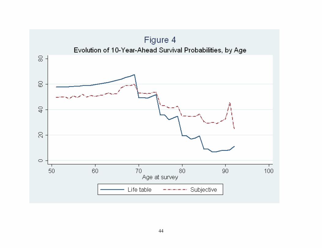
Figure 4 plots the average of these responses as a function of age at the survey date. Two

patterns are immediately apparent from the figure. First, the probability of surviving for 11-15

years declines as the five year age window increases, implying that across individuals, the

subjective mortality hazards are increasing with age. Second, these declines are not as large as

6 Laitner and Silverman (2005) provide an alternative explanation of this “retirement-consumption puzzle” and a

review of much of the recent literature on this phenomenon.

14

those associated with life table survival probabilities. Again, individuals appear to overstate

mortality rates at relatively young ages (up to age 80), and understate mortality rates from age 80

onward.7

Figure 4 suggests that individuals do account for increasing hazard rates with age, which

apparently contradicts the inferences from Tables 1-3. This apparent discrepancy may exist

because one set of findings is generated from the probability beliefs of those under 65 years old,

i.e., two probabilities from someone of a given age, while the other inference comes from a

comparison of individuals at different ages. These age-constant and age-varying estimates may

differ because individuals’ expectations evolve throughout their lifetime, or because successive

cohorts of individuals have different beliefs about their own mortality. We will return to the

second possibility below, but a first cut of the data implies that it does not hold - the average

probability of surviving to a specific age is largely insensitive to cohort effects. For example,

those in their fifties in 1992 and those in their fifties in 2004 report roughly equal probabilities of

survival to age 75. This pattern suggests that the evolution of expectations throughout the life

cycle may play a large role.

The structure of the HRS subjective questions, and their evolution throughout time,

allows for a comparison of individuals’ expectations as they age. As noted above, the

probability of surviving to age 85 conditional on surviving to 75 is indirectly elicited from those

under age 65 in all years. Unfortunately, respondents who are 75 years old never report the

probability of living to age 85, which would provide another estimate of this conditional

probability. However, those aged 70 to 74 are asked this question six times between 1993 and

2004. Subjective probabilities of survival to age 85 for this group will likely slightly understate

7 The overstatement at age 80 onward is much more pronounced for men, but women comprise a large proportion of

the sample at these advanced ages.

15

the 10-year survival probability of 75 year olds, but the bias is likely to be small because the age

gradient of the average age-85 survival probabilities is modest among the 70 to 74 year olds (the

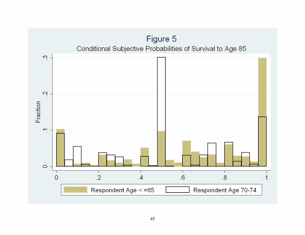
averages are largely insensitive to using responses of 74 year olds only). Figure 5 presents

histograms of the implied conditional values separately for the two groups, those under age 66

and those aged 70 to 74. As is apparent from the figure, the older group is more likely to report

values below 0.5 (except for zero) and less likely to report large values. Much of the difference

appears to be driven by responses of exactly 1, since nearly 30 percent of respondents under 65

reports the same value for P75 and P85. Still, the differences appear lower in the distribution as

well, with the 25th

, 50th

, and 75th

percentiles being 0.3, 0.5, and 0.8 for the 70-74 group and 0.42,

0.7, and 1 for the younger group, respectively. This pattern suggests that individuals do revise

their conditional survival forecasts downward as they age, implying that eventually survival

forecasts reflect increasing age-specific mortality rates.8

IV. Subjective Responses as Predictors of Eventual Mortality

The most appropriate measure of the usefulness of subjective survival probabilities arguably

involves whether they can predict in-sample mortality. Hurd and McGarry (2002) analyzed this

question using the first four waves of the HRS, finding that average values of P75 and P85 are higher

among those who survive until 1998 than among those who do not. The aging of the original HRS

and AHEAD cohorts and the addition of the CODA and WB cohorts uncovers new information

about the relationship between subjective survival probabilities and mortality, including the ability to

precisely assess the accuracy of subjective survival forecasts.

8 The HRS panel is now sufficiently long to allow for a within-individual comparison of these expectations across

age, since the original cohort is 65 to 75 years old in 2006. Analyzing changes across time for the same individuals,

e.g., those aged 56 to 60 in 1992 and aged 70 to 74 in 2006, yields qualitatively similar results but a substantial loss

of precision.

16

Figure 6 displays in-sample average mortality rates by the value sof P75 and P85 reported in

the first wave an individual appeared in the survey.9 Both P75 and P85 appear to predict actual

mortality outcomes well, particularly P75. The in-sample probability of death is monotonically

decreasing as a function of P75 until P75 equals 1.0. Although several authors have suggested that

“focal responses” of 0, 0.5, and 1.0 do not provide any real information to subjective questions, the

implications of the table provide some confidence that they do. Survival rates when P75 = 0 are

lower than for any other value, and rates when P75 = 0.5 are lower than for any value of P75 greater

than 0.5 and greater than for any response less than 0.5. The glaring exception involves P75 values

of 1.0, which are associated with higher mortality rates than any other response above 0.5. A value

of P75 of 1.0 is not pure noise, as the mortality rate for these individuals is lower than the mean death

rate in the sample, but these responses should be viewed with skepticism. Almost all sample

members represented by the table have not yet reached 75, yet more than 10 percent of this group is

deceased. For brevity we do not report the distribution of P75 among survivors and non-survivors,

but the former stochastically dominates the latter, with the density of P75 being lower among

survivors for all values less than 0.5 and greater for all values greater than 0.5.

The 2004 wave of the HRS presents a novel opportunity to study the predictive validity of

subjective survival curves because the original 1993 AHEAD respondents have been in the sample

for eleven years. As such, if their assessments of P10 were accurate, in-sample mortality rates should

be approaching the average assessment. The top panel of Table 4 presents sample averages of P10,

the corresponding life-table averages, and the actual survival rates among these respondents. One

would expect actual survival rates to be greater than both life table and subjective estimates for three

reasons. First, as Hurd et al (1998) notes, life tables may not represent the probability distributions

9 These values of P75 and P85 are not adjusted for the age of the respondent. The pattern of results is robust to such

an adjustment, largely because the values do not vary substantially by age.

17

facing these respondents because the AHEAD did not sample institutionalized individuals, who

presumably have relatively low survival rates. Second, very few of these individuals have reached

the age to which their assessments of P10 apply. For example, a 70-year-old reports the subjective

probability of surviving to age 85, but by 2004, a survivor has only reached age 81. Third, and most

significant, life tables at a point in time do not represent the actual mortality profile facing a

particular cohort if age-specific mortality rates decline over time, as has happened since 1993 - life

table survival rates are higher in 2003 (the last year published life tables were available, as of this

writing) than in 1993. This last limitation does not apply to subjective survival rates but may

substantially affect the interpretation of life tables, especially among cohorts that experienced large

gains in life expectancy.

With these caveats in mind, the patterns shown in Panel A are still informative and largely

mirror those noted above. Specifically, optimism in subjective forecasts increases with age, relative

to life table probabilities. Actual survival rates are higher than either the subjective or the life table

probabilities for ages below 80, but in the 80-84 age group actual survival rates dip below the

subjective probabilities. Among those aged 85-89 in 1995, actual 2004 survival rates are only 8.74

percent, roughly one-fourth the mean value of P10. The conjecture that subjective values of P10 are

more useful than life table values due to sample composition and the ability of individuals to forecast

changes life tables does not appear to be accurate, judging from the accordance with in-sample

mortality.

The bottom panel of Table 4 presents additional evidence about the usefulness of

subjective survival probabilities among older populations. Within each age range, the average

value of P10 is higher among survivors than among those who died, but these differences are

modest and declining with age. Among those under 75 who died by 2004, the average

18

respondent reported a nearly 50 percent likelihood of surviving until at least 2004 (and as long as

2008 for those aged 65 and 70). This evidence is consistent with the notion that subjective

survival forecasts are less accurate for those at the highest end of the age spectrum, possibly

because individuals cannot accurately assess the likelihood of discrete changes in their health

status.

Table 5 presents additional information about the age profile of the association between

subjective survival probabilities and actual in-sample survival rates in the HRS and AHEAD.

The entries represent marginal effects of subjective and life table values of P10 in the wave an

individual entered the sample from probit models of in-sample survival. The first two columns

of the table present estimates among those younger than 65. The coefficient on the subjective

probabilities in the first column is 0.013, with a standard error of 0.001, implying that a 10 point

increase in subjective survival rates is associated with a 1.3 percentage point increase in actual

survival (note that the coefficients have been scaled upward by a factor of 10 for readability).

Similarly, a ten-percentage-point increase in the life table value is associated with a 2.4

percentage point increase in survival. Column (2) adds controls for marital status, race,

ethnicity, living arrangements, assets, income, and body mass index. The controls increase the

explanatory power of the models, as the pseudo-R2 increases from 0.018 to 0.057, but do not

substantially change the coefficient on P10.

Columns (3) and (4) of the table repeat the estimates for those age 65 and over when first

observed. In these two specifications, life table values explain much more of the variation in

survival rates than in the first two columns. This pattern is primarily due to the fact that life table

values vary much more in these age ranges because the target survival age varies across

individuals (recall that the target is 11-15 years from one’s current age among those 65 and over,

19

but constant at 75 for those under age 65). Most importantly, among those over age 65, life table

information has a much stronger association with actual survival than does subjective

information. The (unreported) pseudo- R2 of a specification relating survival to subjective

probabilities is only 0.02, compared to 0.11 in a model including only life table information. For

those over age 64, subjective probabilities apparently do contain information not contained in life

tables, but only a modest amount; moreover, life tables in isolation appear to be stronger

predictors of mortality than subjective values. The addition of covariates does not substantially

change any of the findings

It is worth reemphasizing that life tables at a point in time do not capture the expected

survival outcomes of a particular birth cohort if mortality rates are time varying. Age-specific

mortality rates in the U.S. declined steadily between 1993 and 2003, implying that 1993 life

tables overstate the death rates of individuals between 1993 and 2003. Likewise, 2003 life tables

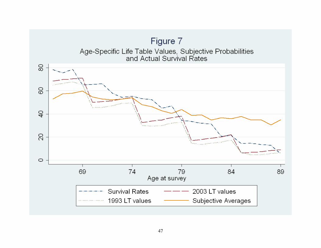
understate these death rates. Figure 7 presents the 1993 values of subjective and life table

probabilities for those in the original 1993 AHEAD sample (as in Figure 4), and adds

information on actual survival rates and 2003 life table values. Among those aged 69, 74, 79, 84,

and 89, the target age in 1993 corresponds to a survivor’s actual age in 2004. The survival

percentages are monotonically decreasing in one’s original age in 1993, consistent with the

increasing age gradient in yearly death rates. More importantly, the actual survival rate of

AHEAD respondents lies between the two life table values for four of the five relevant target

ages; the survival rate among those 74 when originally surveyed is slightly higher than the 2003

life table rate, although this difference is not statistically significant at conventional levels (p =

0.22). This pattern is indicative that the AHEAD cohort is representative of the mortality

experiences of the U.S. population in these ages. As expected, the age profile of the subjective

20

averages is much flatter than either the life table or survival data. The subjective probabilities

under-predict survival by roughly 7 percentage points among 69 year olds in the 1993 AHEAD

and over-predict survival substantially for those in the upper limits of the age range. Again,

these patterns imply that subjective mortality data exhibit systematic biases relative to life tables

and actual survival rates. This apparently discouraging result does not mean that subjective data

are useless in explaining economic behavior, but it suggests that future efforts to understand the

determinants of subjective responses, and the resulting biases, will be fruitful.

V. Updating of Subjective Mortality Forecasts and the Relationship between Cognitive

Ability and Subjective Responses

The biases uncovered above beg the question of how individuals form subjective

probabilities, how they report these probabilities to survey enumerators, and how they update

them in response to new information. A number of previous authors have investigated the role

of new information on individuals’ subjective responses. Hurd and McGarry (2002) and Smith

et al (2001) have noted that probabilities of survival to a given target age do not increase with

age as much as life tables would imply, possibly because health changes are mostly unexpected.

Similarly, Maestas (2006) finds that aggregate subjective measures do not evolve over time in

response to aggregate information.

Table 6 presents evidence on the determinants of changes in subjective measures in the

HRS. In agreement with Maestas’s (2006) findings, the top panel of the table reports sample

average value of P75 and P85 across HRS waves among those aged 55 to 65. The findings are

striking - although life tables evolved substantially during this twelve-year period, subjective

responses remained largely constant. Respondents in 1992 understated the probability of living

21

to age 75, and that bias has grown over time; in 2004, respondents’ average values of P75 were

over 10 percentage points lower than the corresponding life table figures. Panel B shows that

although mortality rates have declined at older ages (80 and 85), subjective responses relevant to

these ages have also stayed roughly constant. These patterns represent a puzzle in the study of

expectations since life tables are publicly available.

The bottom panel of the table presents estimates of the determinants of the within-person

evolution of survival probabilities as an individual ages, both subjective and objective. The

estimates reported are coefficients from regressions of survival probabilities on the respondent’s

age, including individual fixed effects. The first column essentially replicates the findings of

Hurd and McGarry (2002), as it shows that subjective survival probabilities are insensitive to

age. The top point estimate of 0.01 implies that each year of age is associated with an increase in

average values of P75 of only 0.01 of a percentage point; in contrast, the life table probability

increases by 0.91 percentage points. The findings for P85 are similar, in that that age does not

significantly affect the subjective measures but dramatically affects life tables. The second

column adds indicators for objective measures of health, such as diagnoses of chronic diseases

and difficulties with activities of daily living. The estimates associated with life tables do not

change, since life tables do not account for this information, but the estimates associated with P75

and P85 increase. Column (3) adds one additional control, an individual’s self-reported health

status (on a scale of 1 to 5). In this final specification, the subjective estimates increase

dramatically relative to column (1), although in the case of P75 the estimate lies far below the life

table estimate. A comparison across columns confirms that the subjective measures do not

embody the possibility of future health shocks, i.e., health declines among the near-elderly

22

appear to be largely unexpected. Individuals do, however, revise their forecasts in the presence

of these shocks, especially with longer planning horizons.

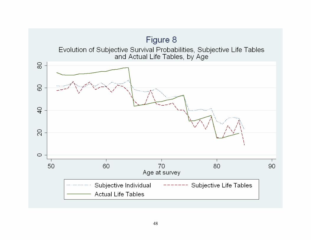
The 2006 wave of the HRS provides a unique opportunity to evaluate the determinants of

responses of subjective probabilities to new information. The insensitivity of subjective

measures to life tables implied by the top panels of Table 6 suggests that knowledge of life tables

may not affect subjective survival probabilities, but a special module administered to 10% of

2006 sample respondents elicited information intended to directly assess this relationship. In

particular, after individuals reported their subjective measures, they were asked a question

designed to measure their knowledge of life tables:

“Out of a group of 100 [men/women] your age, how many do you think will survive to

the age of X?”

As in the subjective probabilities themselves, the value of X depends on the current age of the

respondent; it is equal to 75 for all those under age 65, 80 for those aged 65-69, 85 for those aged

70-74, and so on. After answering this question, the respondent is told the corresponding 2003

life table value:

“Now, suppose I told you that according to statistics, on average about [#] out of 100

[men/women] your age should live to age X.”

After being read the actual life table value, the respondent is then asked again for his or her

subjective survival probability. Ascertaining whether this updated value is related to the

updating of life table information is of particular interest, so we construct two measures, the first

being the difference between the two subjective probabilities, and the second being the

difference between the subjective life table estimate and the actual life table value.

23

Before turning to the determinants of updating, it is informative to examine the responses

themselves. Figure 8 presents the average value of the subjective individual probabilities, the

“subjective life tables”, and the actual life tables, by age. The subjective probabilities are flatter

than the life table rates, as noted above, and interestingly, so are the average subjective life table

probabilities. It appears that the subjective individual probabilities and subjective life tables

track each other closely, with the individual probabilities being on average higher at every age

(the exceptions are ages 56 and 58); the differences in the averages are statistically significant (p

< 0.001). The differences between actual and subjective life tables before age 65 imply that, on

average, the near elderly are largely unaware of actual life table values.

Given that individuals appear to err systematically in assessing life table probabilities,

particularly at younger ages, one might speculate that the presence of actual life table data would

substantially change assessments of individual survival probabilities. Table 7 presents evidence

that this conjecture is incorrect. The estimates in the table are linear OLS estimates of the effect

of updates in life tables on updates in subjective individual survival rates. Column (1) shows

that a 1-point increase in life tables is associated with only a 0.034 point increase in subjective

probabilities among those under age 65. This is particularly surprising, given that this group’s

average assessment of life table survival rates was roughly 10 points lower than actual life table

averages. Column (2) adds the value of the original subjective value as a regressor. The

estimates in this column imply that the subjective values are strongly mean reverting, since a 1-

point increase in the original response is associated with a 0.537-point decrease in the update.10

The estimate associated with the life table update becomes negative; the reduction in the

magnitude of this estimate is due to the negative association between the original subjective

10

This mean reversion is not surprising, since the support of the survival probabilities is restricted to be within the 0-

1 interval. Limiting the sample to those whose original response was between 30 and 70, for example, reduces the

point estimate’s magnitude but does not eliminate it.

24

value and the life table update, resulting from the positive association between the original life

table estimate and the original subjective estimate.

The remaining columns in Table 7 present similar findings for those aged 65 and older,

namely, that the updates in life tables and subjective probabilities are unrelated unconditionally

and negatively related conditional on the value of the original subjective estimate. Figure 9

presents graphical evidence of the lack of correlation between the two updates. Each circle

corresponds to a value of the life table update, ranging from -69 to 81, and the size of the circle

represents the number of individuals associated with that value. The estimated simple linear

regression line is overlaid on the figure. Taken together, Table 7 and Figure 9 present

compelling evidence that subjective beliefs about life tables and individual subjective

probabilities are correlated because individuals use their beliefs about their own mortality

experience to form beliefs about the population, not vice versa. These findings imply that

systematic biases in subjective probabilities may still exist even if all individuals had perfect

knowledge of life tables.

The Role of Cognition

Previous studies have established a relationship between subjective beliefs and measures

of cognition available in the HRS. In particular, cognitive skills are positively associated with

subjective survival probabilities. The cause of this association is unclear because those with high

cognitive functioning are presumably likely to live to older ages, but they also might be

relatively more able to form accurate probability assessments. Separating these two pathways is

a difficult task, but the multiple questions in the HRS suggest a possible avenue. In particular, if

a better understanding of probability assessments is the driving force, one might suspect that the

flatness in implied yearly hazards found above would be less pronounced among those with high

25

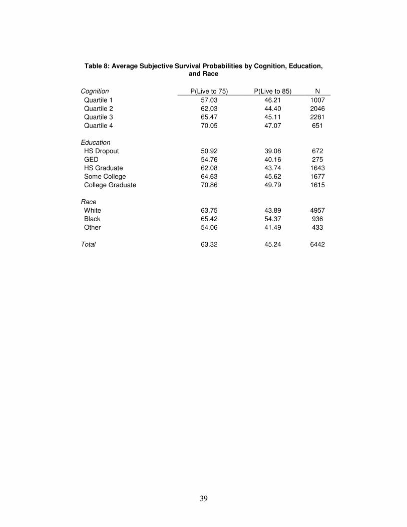
cognitive functioning. Table 8 presents striking evidence that this is the case. We have

classified individuals into one of four categories based on their responses to questions in the

“Cognition” section of the HRS.11

These measures are powerfully correlated with P75 but not

P85. The negative bias in subjective assessments of P75 appears to be much larger among those in

the lowest cognitive quartile. Alternatively, the negative bias may be constant across quartiles if

actual survival rates are much higher among those in quartile four, but if that were the case, one

would expect a positive association between cognition and P85. Although these figures are only

suggestive, they are consistent with the notion that those with higher cognition have greater

survival rates and more accurate assessments of these rates.

The cognitive measures in the HRS are limited in scope, and as argued above, the

association between them and survival assessments are subject to problems of interpretation. In

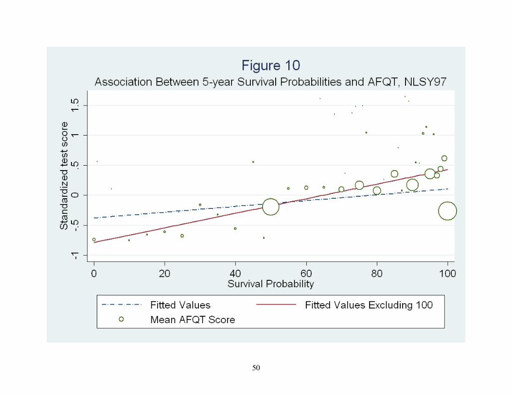
order to further assess the role of cognition in forming beliefs about survival, we use information

from another data set, the National Longitudinal Survey of Youth-1997 (NLSY97), which elicits

5-year survival assessments from a sample of youths aged 13 to 16. An advantage of the

NLSY97 lies in the availability of a detailed set of measures of cognition, particularly scores on

the Armed Forces Qualifying Test (AFQT). Figure 10 shows the association between survival

probabilities and standardized AFQT scores, with the size of a circle again indicating the number

of respondents who reported a particular survival probability. As in the HRS, cognition and

survival beliefs are strongly positively correlated, with the value of 100 being an exception. Life

table survival rates for this group are roughly 99.8% and do not drop below 95% for any race or

gender, so a response of under 80 percent is likely to reflect a mistake or a fundamental lack of

knowledge about survival probabilities. Put another way, the association between cognition and

11

These assessments include measures of immediate and delayed word recall, questions such as “who is the

president of the United States”, and questions designed to elicit arithmetic ability such as, “if 5 people all have the

winning numbers in the lottery and the prize is two million dollars, how much will each of them get?”

26

survival probabilities in these data does not reflect a genuine association between actual survival

rates and ability. The findings in the NLSY and the HRS suggest that cognition and measures

like P75 may be correlated for reasons distinct from actual mortality. As a result, correlations

between subjective probabilities and economic outcomes may operate solely through cognitive

ability.

VI. Subjective Mortality Forecasts and Portfolio Choice

Economists are primarily interested in subjective beliefs about survival to the extent that

they affect economic behavior such as savings and consumption, claiming of Social Security

benefits, asset accumulation and portfolio choice, and bequests. The preceding sections’ key

lessons imply that uncovering these relationships is difficult in practice for many reasons,

including systematic biases in survival beliefs, spurious correlations between beliefs and

outcomes due to unmeasured cognitive ability, and measurement error in forecasts. Indeed,

many authors have failed to find a relationship between subjective forecasts and outcomes that

should exist according to economic theory. For example, Perry (2005) finds no evidence of an

association between subjective mortality and asset decumulation after retirement, Bloom et al

(2006) finds mixed evidence on the relationship between beliefs and retirement or asset levels,

and Hurd et al (1998) find mixed evidence on the effect of beliefs on the timing of Social

Security claiming.

In this section, we will attempt to quantify the relationship between mortality forecasts

and portfolio allocation decisions. Portfolio theory posits that as an individual’s planning

horizon lengthens, the individual should become more tolerant to volatility in year-to-year

returns. In the context of the HRS, this implies that those with higher subjective survival rates

27

should hold a riskier portfolio of assets, all else constant. The empirical difficulty in holding “all

else constant” lies in the likely correlation between determinants of responses to subjective

probability questions and unobservable factors that affect portfolio choice. Consider the top

panel of Table 9. Column (1) presents one measure of a portfolio’s volatility, the proportion of

wealth invested in stocks and mutual funds, across 11 categories of the range of P75. It is

apparent that this proportion rises nearly monotonically with P75, with those giving a value of

100 (or 1.0, if measured on a 0-1 scale) being the exception. The discussion above implies that

this pattern, particularly the dip at 100, may be entirely due to cognitive skills that are

presumably correlated with asset allocation decisions - those with higher cognitive function may

be more perceptive investors who have the skills and financial literacy needed to invest in the

stock market.

In order to attempt to untangle the various reasons underlying the correlation between the

proportion of wealth invested in stocks and survival forecasts, we proceed in two steps. In the

first, we estimate nonparametric lowess-smoothed models of the relationship between the stock

proportion and total asset holdings. This procedure involves a locally weighted linear regression

for each observation in the sample to generate smooth estimates of the proportion of wealth

invested in stocks as a function of total wealth holdings. If one is willing to maintain the

assumption that total wealth is a sufficient statistic for the unobservable determinants of asset

allocation decisions, the smoothed values of this relationship will encompass these

unobservables. These predicted values are shown in column (2) of the table, and they exhibit a

positive correlation with P75, implying that those with more optimistic survival forecasts also

have greater overall wealth holdings. These smoothed values will be orthogonal to the

component of survival probabilities that is unrelated to total wealth holdings; this orthogonal

28

component is shown in the third column, which is simply the difference between the first two

columns. This column shows that variation in subjective survival probabilities that is unrelated

to total wealth holdings is still positively related to portfolio volatility, although less so than is

the total variation in survival probabilities. In particular, those with values of P75 between 90 and

99 are estimated to have roughly 3.2 percent more of their assets invested in stocks and mutual

funds than those with values of P75 between 50 and 59. Again, the relationship appears nearly

monotonic apart from those with P75 equal to 100.

Panel B of Table 9 presents OLS estimates of the effect of subjective and life table values

of P75 on the stock proportion. The first two columns present naïve OLS estimates, with the key

finding from these results being that the point estimates are quite sensitive to the inclusion of

additional covariates such as education, race, and household composition; the estimate of interest

declines from 0.111 to 0.049 once these controls are included. Evidently, the subjective

probabilities are correlated with observable factors related to stock ownership, which highlights

the possibility that they are also correlated with the unobservable determinants. Columns (3) and

(4) present estimates with the residuals from the lowess models as dependent variables. The

estimates on the subjective P75 are much less sensitive to the inclusion of controls in this case,

providing some reassurance that the procedure is robust to unobserved heterogeneity in the

propensity to own stocks. The preferred estimate, in column (4), implies that a 100 percent

increase in P75 increases the proportion of one’s assets held in stocks and mutual funds by 2.1

percentage points, a modest effect relative to the naïve OLS estimates. Still, this value is

statistically different from zero at conventional significance levels. Although the magnitude of

this estimate is of marginal economic significance, it does imply that survival probabilities

29

influence economic behavior - we tentatively conclude that subjective survival probabilities

increase investor tolerance for risk.

VII. Conclusions

This paper has presented evidence on the nature of subjective survival probabilities in the

Health and Retirement Study, with a focus on these measures’ usefulness as predictors of actual

mortality and economic behavior. We find that observed mortality forecasts exhibit systematic

biases relative to life table data, and that these biases are not due to individuals correctly

forecasting future changes in life tables. Average subjective survival probabilities show signs of

substantial pessimism relative to life tables about the likelihood of survival to relatively young

ages, and equally sizeable optimism about the probability of survival to more advanced ages,

particularly age 85 and beyond. On average, HRS respondents aged 50 to 64 do not appear to

account for the positive age gradient in yearly death rates. In contrast, older individuals

eventually revise their conditional survival forecasts downward as they age.

Subjective survival probabilities predict in-sample mortality well at younger ages, but

less so past age 65. Among HRS respondents over age 75, initial survival forecasts among those

who survive until 2004 are only modestly different from those of sample members who die by

2004. For all age groups, life table survival probabilities predict in-sample survival at least as

well as subjective probabilities, with the relative predictive power of life tables being much

greater among those over age 65. Given this finding, it is puzzling that individuals do not

modify their expectations in response to changes in life tables, even when life table data are

directly given to them, as in the 2006 HRS module on health and mortality expectations.

Cognitive ability appears to be a big part of the story, as those with greater measured

30

mathematical acuity report relatively more accurate subjective data that is more consistent with

the age profile of mortality rates. “Focal responses” of 0, 50, and 100 percent have received

attention in the literature as a measure of forecasting accuracy, but only responses of 100 percent

appear to be difficult to interpret. Across a wide variety of survival and economic outcomes,

those who report a 100 percent likelihood of survival appear fundamentally different from those

who report probabilities in the 80s and 90s.

Finally, we have documented the difficulties inherent in interpreting correlations between

subjective survival probabilities and economic outcomes as causal effects. Survival forecasts are

likely to be correlated with unobservable determinants of outcomes such as the timing of OASDI

benefit claiming, retirement, and the dynamics of asset holdings following retirement. In spite of

these difficulties, we tentatively conclude that optimism in longevity increases an individual’s

tolerance for short-run volatility in investment returns, as measured by the proportion of wealth

invested in stocks and mutual funds. There is a large scope for future research relating

subjective expectations to economic outcomes, and the principal goal in this area will involve

advances in credible methods for identifying the causal effects of interest.

31

References

Bloom, D. E., D. Canning, M. Moore and Y. Song (2006). "The Effect of Subjective Survival

Probabilities on Retirement and Wealth in the United States," Working Paper 12688,

National Bureau of Economic Research.

Hamermesh, D. (1985), "Expectations, Life Expectancy, and Economic Behavior," Quarterly

Journal of Economics, 100, 389-408.

Harris, C., and D. Laibson (2001), "Dynamic Choices of Hyperbolic Consumers," Econometrica,

69, 935-957.

Hurd, M., and K. McGarry (1995), "Evaluation of the Subjective Probabilities of Survival in the

Health and Retirement Study," Journal of Human Resources, 30, S268-S292.

Hurd, M., and K. McGarry (2002), "The Predictive Validity of Subjective Probabilities of

Survival" Economic Journal, 112, 966-98.

Hurd, M., J. Smith, and J. Zissimopoulos (2002), "The Effects of Subjective Survival on

Retirement and Social Security Claiming," Working Paper 9140, National Bureau of

Economic Research.

Kézdi, G., and R. Willis (2003), "Who Becomes A Stockholder? Expectations, Subjective

Uncertainty, and Asset Allocation," Working Paper 2003-039, Michigan Retirement

Research Center.

Laitner, J, and D. Silverman (2005), "Estimating Life-Cycle Parameters from Consumption

Behavior at Retirement," Working Paper 11163, National Bureau of Economic Research.

Lillard, L. and R. Willis (2001), "Cognition and Wealth: The Importance of Probabilistic

Thinking," Working Paper 2001-007, Michigan Retirement Research Center.

Maestas, N., "Cohort Differences in Retirement Expectations and Realizations," Working Paper

2006-13, Pension Research Council.

Manski, C. (2004), "Measuring Expectations," Econometrica, 72, 2004, pp. 1329-1376.

Perry, M. (2005), "Estimating Life-Cycle Effects of Subjective Survival Probabilities in the

Health and Retirement Study," Working Paper No. 2005-103, Michigan Retirement

Research Center.

Smith, V. K., D. Smith, D. H. Taylor, Jr., and F. Sloan (2001), "Longevity Expectations and

Death: Can People Predict Their Own Demise?" American Economic Review, 91, pp.

1126-1134.

32

Table 1: Distribution of Subjective Probabilities of Living to Age 75 or 85

Panel A: Age 75

All Male Female

Age range Subjective LT Subjective LT Subjective LT

<50 64.46 71.41 56.05 60.65 66.12 73.61

50-54 64.68 69.83 61.44 61.80 66.56 74.75

55-60 64.72 71.13 63.01 64.26 65.97 76.53

60-64 65.40 74.62 64.24 69.00 66.37 79.56

65 66.88 77.97 66.61 73.63 67.16 82.57

Panel B: Age 85

All Male Female

Subjective LT Subjective LT Subjective LT

<50 44.95 42.00 36.62 26.62 45.97 43.88

50-54 43.34 38.11 39.16 27.25 45.82 44.55

55-60 42.48 38.10 39.13 28.62 45.12 45.57

60-64 42.91 39.26 40.36 30.66 45.25 47.18

65 48.13 37.67 47.51 33.45 49.82 49.29

33

Table 2: Distribution of Subjective Probabilities of Living to Age 75 or 85

Panel A: Age 75

Age range 0 0.01-0.49 0.5 0.51-0.99 1 N

<50 6.28 11.57 22.63 40.79 18.72 3199

50-54 5.88 11.75 23.64 39.77 18.96 14251

55-60 5.94 11.51 24.15 38.25 20.14 21318

60-64 5.26 10.98 24.97 38.05 20.74 19965

65 3.89 10.39 26.6 36.85 22.28 2985

Panel B: Age 85

Age range 0 0.01-0.49 0.5 0.51-0.99 1 N

<50 15.75 31.4 18.23 26.52 8.1 2172

50-54 16.49 32.71 18.78 23.09 8.92 9739

55-60 17.23 33.21 18.9 21.7 8.97 14385

60-64 16.77 33.16 19.14 21.31 9.63 10885

65 13.93 26.98 21.95 25.73 11.41 2068

34

Table 3: Tests of the Constant Hazard Hypothesis

Estimation Method

Implied by Constant hazard rate

Life Table

OLS 2SLS 2SLS OLS

Age N (1) (2) (3) (4) (5)

50 908 1.17 1.44 1.27 2.33 1.40

(0.04) (0.08) (0.26)

55 2359 1.18 1.65 1.52 2.43 1.50

(0.03) (0.06) (0.18)

60 2300 1.17 1.47 2.47 2.62 1.67

(0.03) (0.06) (0.64)

61 2109 1.15 1.43 1.56 2.68 1.71

(0.03) (0.06) (0.21)

62 1783 1.08 1.63 1.95 2.73 1.77

(0.03) (0.08) (0.33)

63 1573 1.17 1.67 1.80 2.82 1.83

(0.03) (0.06) (0.26)

64 1277 1.10 1.32 2.13 2.91 1.91

(0.03) (0.06) (0.48)

65 728 1.12 1.57 1.95 3.03 2.00

(0.04) (0.09) (0.33)

Note: The entries for each model are the coefficient, and standard error in parentheses, from linear mean regressions of log(P85) on log(P75). Column 1 is estimated via OLS, column 2 uses other-period average values of P75 as instruments for P75, and column 3 uses saturated indicators of parental age and mortality as instruments. Standard errors are adjusted for clustering at the individual level.

35

Table 4: Sample Mean Probabilities of Living 11 to 15 More Years and Survival Rates, by in-Sample Mortality Status - Men

Panel A: Means of P10 and 11-year survival rates

P10

Age range Subjective Life Table Actual Survival Rate N

65-69 53.57 51.31 71.12 606

70-74 51.15 36.81 56.11 2274

75-79 38.26 21.32 41.79 1610

80-84 33.26 9.22 25.06 1080

85-89 31.42 3.33 8.74 502

Panel B: P10 by 11-year Mortality Status

Survivors Non-Survivors

Age range Subjective Life Table Subjective Life Table

65-69 58.66 51.75 46.92 50.73

70-74 52.65 36.70 49.23 36.95

75-79 43.00 21.42 34.86 21.25

80-84 35.50 8.96 32.51 9.30

85-89 33.75 3.85 31.20 3.28

36

Table 5: The Association Between Subjective and Life Table Survival Probabilities and In-Sample Mortality, by Age

Under Age 65: Over Age 65:

(1) (2) (3) (4)

Subjective 0.013 0.011 0.014 0.014

(0.001) (0.001) (0.001) (0.001)

Life Table 0.024 -0.005 0.081 0.071

(0.003) (0.001) (0.002) (0.003)

Additional Controls? No Yes No Yes

R2 0.018 0.057 0.122 0.137

N 29,879 29,879 11,164 11,164

Note: The entries in each column are marginal effects from probit models of actual within-sample survival in the HRS. The coefficients and associated standard errors are multiplied by 10 for each of interpretation. Columns (2) and (4) include additional controls as described in the text. Standard errors are adjusted for clustering at the individual level.

37

Table 6: Sample Mean Probabilities of Living to 75 and 85 among those aged 55-65, by HRS Wave

Panel A: Age 75

Wave Subjective Life Table N

1992 64.21 70.20 6114

1994 63.62 71.24 6390

1996 64.90 72.44 7164

1998 65.18 73.35 6637

2000 66.55 74.60 6264

2002 66.27 75.87 5794

2004 65.40 76.23 5597

Panel B: Age 85 (80 after 1998)

Wave Subjective Life Table N

1992 42.36 37.31 6103

1994 41.10 37.92 6376

1996 44.20 39.09 7205

1998 43.21 40.04 6546

2000 51.12 59.49 6190

2002 51.40 60.92 5744

2004 51.61 61.47 5552

Panel C: Within-Respondent Estimates of the Effect of Age on Subjective and Life-Table Survival Rates

Control Set

N

Outcome (Unique) (1) (2) (3)

P75

Subjective 51730 0.01 0.10 0.18

(16811) (0.04) (0.03) (0.03)

Life Table 0.91 0.91 0.91

(0.01) (0.01) (0.01)

P85

Subjective 29040 0.03 0.47 0.60

(13573) (0.06) (0.09) (0.09)

Life Table 0.60 0.61 0.61

(0.03) (0.06) (0.06)

38

Table 7: Determinants of Updating of Subjective Survival Probabilities

Under Age 65: Over Age 65:

(1) (2) (3) (4)

Life Table Update 0.034 -0.175 -0.013 -0.171

(0.044) (0.035) (0.060) (0.049)

Original Subjective Value … -0.537 … -0.515

… (0.026) … (0.033)

R2 0.010 0.417 0.001 0.349

N 590 590 712 712

39

Table 8: Average Subjective Survival Probabilities by Cognition, Education, and Race

Cognition P(Live to 75) P(Live to 85) N

Quartile 1 57.03 46.21 1007

Quartile 2 62.03 44.40 2046

Quartile 3 65.47 45.11 2281

Quartile 4 70.05 47.07 651

Education

HS Dropout 50.92 39.08 672

GED 54.76 40.16 275

HS Graduate 62.08 43.74 1643

Some College 64.63 45.62 1677

College Graduate 70.86 49.79 1615

Race

White 63.75 43.89 4957

Black 65.42 54.37 936

Other 54.06 41.49 433

Total 63.32 45.24 6442

40

Table 9: Estimates of the Effect of Subjective Survival Probabilities on Portfolio Riskiness

Panel A: Proportion of Wealth in Stocks by Value of Age-75 Survival Probabilities

Range of P75 Raw Proportion

(1) Predicted (2) Difference (1-

2) N

0-9 0.094 0.098 -0.003 2489

10-19 0.112 0.113 -0.001 1118

20-29 0.120 0.123 -0.003 1594

30-39 0.141 0.127 0.015 979

40-49 0.124 0.126 -0.002 1003

50-59 0.138 0.138 0.000 11273

60-69 0.167 0.150 0.017 1841

70-79 0.177 0.155 0.022 5610

80-89 0.182 0.157 0.025 6290

90-99 0.191 0.159 0.032 3518

100 0.146 0.135 0.011 8954

Total 0.152 0.140 0.012 44,669

Panel B: Estimates of Causal Effects

Naïve OLS Estimates: Adjusted for Wealth Holdings:

(1) (2) (3) (4)

Subjective 0.111 0.049 0.028 0.021

(0.005) (0.005) (0.004) (0.005)

Life Table -0.092 0.024 0.091 -0.163

(0.023) (0.070) (0.094) (0.063)

Additional Controls? No Yes No Yes

R2 0.008 0.137 0.003 0.008

N 44,669 44,669 44,669 44,669

Note: The entries in each column in Panel B are coefficients from OLS models of the proportion of assets invested in stocks in the HRS. The coefficients and associated standard errors are multiplied by 100 for ease of interpretation. Columns (2) and (4) include additional controls as described in the text. Standard errors are adjusted for clustering at the individual level. In columns (3) and (4), the dependent variable is the residual from a smoothed lowess estimate of the proportion of wealth invested in stocks as a function of wealth levels.

subjective survival probabilities in the health and - deep blue

Documents