- 31 -

Tech. Rept. SOCS-88.10, McGill University, May 1988.

[To88d] Toussaint, G. T., “Separating two simple polygons by a single translation,”Journal ofDiscrete and Computational Geometry, in press, 1988.

[To88e] Toussaint, G. T., “Polygons are anthropomorphic,” inSnapshots of Computational andDiscrete Geometry, G. T. Toussaint,ed., Tech. Rept. SOCS-88.11, McGill University,June 1988, pp. 1-6.

[To88f] Toussaint, G. T., “Shortest path solves translation separability of polygons,” Tech.Rept. SOCS-85.27, School of Computer Science, McGill University, October 1985.

[TA] Toussaint, G. T. and Avis, D., “On a convex hull algorithm for polygons and its appli-cation to triangulation problems,”Pattern Recognition, vol. 15, No. 1, 1982, pp.23-29.

[TV88] Tarjan, R. E. and Van Wyk, C. J., “An O(n log log n)-time algorithm for triangulatingsimple polygons,”SIAM Journal on Computing, 1988.

- 30 -

Press, 1983, pp. 534-571.

[SK76] Sklansky, J. and Kibler, D. F., “A theory of nonuniformly digitized binary pictures,”IEEE Transactions on Systems, Man, and Cybernetics, Vol. SMC-6, Sept. 1976, pp.637-647.

[SS84] Sharir, M., and Schorr, A., “On shortest paths in polyhedral spaces,” Proc. SixteenthAnnual ACM Symposium in the Theory of Computing, Washington, 1984, pp. 144-153.

[ST88a] Shermer, T., and Toussaint, G. T., “Anthropomorphic polygons can be recognized inlinear time,” in Snapshots of Computational and Discrete Geometry, G. T. Toussaint,ed., Tech. Rept. SOCS 88.11, McGill University, June, 1988, pp.7-14.

[ST88b] Shermer, T., and Toussaint, G. T., “Characterizations of star-shaped polygonal sets,”manuscript in preparation.

[Su87a] Suri, S., “Minimum link paths in polygons and related problems,” Ph.D. thesis, TheJohns Hopkins University, August 1987.

[Su87b] Suri, S., “The all-geodesic-furthest neighbors problem for simple polygons,” Proc.Third Annual ACM Symposium on Computational Geometry, University of Waterloo,June 1987, pp. 64-75.

[Su86a] Suri, S., “Computing the geodesic diameter of a simple polygon,” Tech. Rept. JHU-EECS-86-08, Johns Hopkins University, 1986.

[Su86b] Suri, S., “A linear time algorithm for minimum link paths inside a simple polygon,”Computer Vision, Graphics, and Image Processing, Vol. 35, 1986, pp. 99-110.

[To85] Toussaint, G. T., “A historical note on convex hull finding algorithms,” Pattern Reco-gnition Letters, Vol. 3., January 1985, pp. 21-28.

[To86a] Toussaint, G. T., “Shortest path solves edge-to-edge visibility in a polygon,” PatternRecognition Letters, Vol. 4, July 1986, pp. 165-170.

[To86b] Toussaint, G. T., “A linear-time algorithm for solving the strong hidden-line problemin a simple polygon,” Pattern Recognition Letters,1987.

[To86c] Toussaint, G. T., “An optimal algorithm for computing the relative convex hull of a setof points in a polygon,” Signal Processing III: Theories and Applications, Proc. ofEURASIP-86, Part 2, North-Holland, September 1986, pp. 853-856.

[To87] Toussaint, G. T., “Relative convex hulls of sets and their applications,” IFIP Confer-ence on Modeling and Simulation, Tokyo, September 1987.

[To88a] Toussaint, G. T., Editor, Computational Morphology, North-Holland, 1988.

[To88b] Toussaint, G. T., “A geodesic Helly-type theorem,” in Snapshots of Computational andDiscrete Geometry, G. T. Toussaint, ed., Tech. Rept. SOCS 88.11, McGill University,June, 1988, pp.135-137.

[To88c] Toussaint, G. T., “An output-complexity-sensitive polygon triangulation algorithm,”

- 29 -

sis,” Pattern Recognition, Vol. 17, 1984, pp. 177-187.

[LP84] Lee, D. T., and Preparata, F. P., “Euclidean shortest paths in the presence of rectilinearbarriers,” Networks, Vol. 14, No. 3., 1984, pp. 393-410.

[LPSSSSTWY] Lenhart, W., Pollack, R., Sack, J., Seidel, R., Sharir, M., Suri, S., Toussaint, G. T.,Whitesides, S., and Yap, C., “Computing the link center of a simple polygon,” Proc.Third Annual ACM Symposium on Computational Geometry, University of Waterloo,June 1987, pp. 1-10.

[MA79] McCallum, D. and Avis, D., “A linear algorithm for finding the convex hull of a simplepolygon,” Information Processing Letters, Vol. 9., 1979, pp. 201-206.

[Me83] Megiddo, N., “Linear-time algorithms for linear programming in R3 and related prob-lems,” SIAM Journal of Computing, Vol. 12, 1983, pp. 759-776.

[ML84] Maisonneuve, F., and Lantuejoul, C., “Geodesic convexity,” Acta Stereologica, Vol. 3,No. 2, 1984, pp. 169-174.

[Mo84] Mount, D. M., “On finding shortest paths on convex polyhedra,” Technical Report,Computer Science Dept., University of Maryland, October 1984.

[PeSa] Peshkin, M. A., and Sanderson, A. C., “Reachable grasps on a polygon: the convex ropealgorithm,” Teck. Rept. CMU-RI-TR-85-6, Carnegie-Mellon University, 1985, alsoIEEE Transactions on Robotics and Automation, in press.

[PS85] Preparata, F. P. and Shamos, M. I., Computational Geometry, Springer-Verlag, NewYork, 1985.

[PS86] Pollack, R., Sharir, M., “Computing the geodesic center of a simple polygon,” in Proc.Workshop on Movable Separability of Sets, G. Toussaint, ed., Bellairs Research Insti-tute, Barbados, February 1986.

[PSR89] Pollack, R., Sharir, M., and Rote, G., “Computing the geodesic center of a simple poly-gon,” Journal of Discrete and Computational Geometry, Vol.4, No. 6, 1989, pp. 611-626.

[PSS88] Pollack, R., Sharir, M., and Sifrony, S., “Separating two simple polygons by a sequenceof translations,” Journal of Discrete and Computational Geometry, Vol. 3, 1988, pp.123-136.

[RS85] Reif, J. and Storer, J., “minimizing turns for discrete movement in the interior of a poly-gon,” Tech. Rept., Harvard University, December 1985.

[SCH72] Sklansky, J., Chazin, R. L., and Hansen, B. J., “Minimum perimeter polygons of digi-tized silhouettes,” IEEE Transactions on Computers, Vol. C-21, March 1972, pp. 260-268.

[SGB83] Suss, W., Gercke, H., and Berger, K. H., “Differential geometry of curves and surfac-es,” in Fundamentals of Mathematics: Vol. II, Geometry, H. Behnke, et al., eds., MIT

- 28 -

York, 1947.

[Dy86] Dyer, M. E., “On a multidimensional search technique and its applications to the Eu-clidean one-center problem,” SIAM Journal of Computing,Vol. 15, 1986, pp. 725-738.

[El85] ElGindy, H., “Hierarchical decomposition of polygons with applications,” Ph.D. Dis-sertation, School of Computer Science, McGill University, 1985.

[El86] ElGindy, H., “A parallel algorithm for the shortest path problem in monotone poly-gons,” Tech. Rept. MS-CIS-86-49, Dept. Computer Science, University of Pennsylva-nia, June 1986.

[EG88] ElGindy, H., and Goodrich, M., “Parallel algorithms for shortest path problems in poly-gons, “The Visual Computer, Vol 3, 1988, pp. 371-378.

[ET89] ElGindy, H., and Toussaint, G. T., “On geodesic properties of polygons relevant to lin-ear time triangulation,” The Visual Computer, in press, 1989.

[ET88] ElGindy, H., and Toussaint, G. T., “On triangulating palm polygons in linear time,”Computer Graphics’88,Geneva, June 1988.

[Eu1728] Euler, L., “On the shortest line on an arbitrary surface connecting any two points what-soever,” Commentary of the Imperial Academy of St. Petersburg, 1728.

[FA84] Franklin, W. Randolph and Akman, Varol, “Shortest paths between source and goalpoints located on/around a convex polyhedron,” Proc. Twenty-Second Annual AllertonConference, Monticello, Illinois, October 1984, pp. 103-112.

[Gh86] Ghosh, S. K., “Computing the visibility polygon from a convex set,” Tech. Rept. CS-TR-1749, University of Maryland, December 1986.

[Gh87] Ghosh, S. K., “A few applications of the set-visibility algorithm,” Tech. Rept. CS-TR-1797, University of Maryland, March 1987.

[GH87] Guibas, L., and Herschberger, J., “Optimal shortest path queries in a simple polygon,”Proc. Third Annual ACM Symposium on Computational Geometry,University of Wa-terloo, June 1987, pp. 50-63.

[GHLST] Guibas, L., Herschberger, J., Leven, D., Sharir, M., Tarjan, R.E., “Linear time algo-rithms for visibility and shortest path problems inside triangulated simple polygons,”Algorithmica, Vol. 2, 1987, pp. 209-233.

[GJPT] Garey, M. R., Johnson, D. S., Preparata, F. P. and Tarjan, R. E., “Triangulating a sim-ple polygon,” Information Processing Letters, vol. 7, 1978, pp.175-179.

[Ki83] Kirkpatrick, D., “Optimal search in planar subdivisions,” SIAM Journal of Computing,Vol. 12, No. 1., February 1983, pp. 28-35.

[LB81] Lantuejoul, Ch. and Beucher, S., “On the use of the geodesic metric in image analysis,”Journal of Microscopy, Vol. 121, January 1981, pp. 39-49.

[LM84] Lantuejoul, C., and Maisonneuve, F., “Geodesic methods in quantitative image analy-

- 27 -

Conference on Modeling and Simulation, Tokyo, September 1987 [To87].

References

[AA] Asano, Te. and Asano, Ta., “Voronoi diagram for points in a simple polygon,” Tech.Rept., Osaka Electro-Communication University, 1986.

[Ar87] Aronov, B., “On the geodesic Voronoi diagram of point sites in a simple polygon,”Proc. Third Annual ACM Symposium on Computational Geometry, University of Wa-terloo, June 1987, pp. 39-49.

[AFW] Aronov, B., Fortune, S., and Wilfong, G., “The furthest-site geodesic Voronoi dia-gram,” Proc. Fourth Annual ACM Symposium on Computational Geometry, Universityof Illinois, June 1988, pp. 229-240.

[AT85] Asano, T. and Toussaint, G. T., “Computing the geodesic center of a simple polygon,”Technical Report SOCS-85.32, McGill University, 1985.

[AT86] Asano, T. and Toussaint, G. T., “Computing the geodesic center of a simple polygon,”in Perspectives in Computing: Discrete Algorithms and Complexity, Proc. of Japan-USJoint Seminar, D. S. Johnson, A. Nozaki, T. Nishizeki, H. Willis, eds., June 1986, pp.65-79.

[ATB82] Avis, D., Toussaint, G. T., and Bhattacharya, B. K., “On the multimodality of distancesin convex polygons,” Computers and Mathematics with Applications, Vol. 8, No. 2.,1982, pp. 153-156.

[Av82] Avis, D., “On the complexity of finding the convex hull of a set of points,” DiscreteApplied Mathematics, Vol. 4, 1982, pp. 81-86.

[BS85] Baltsan, A., and Sharir, M., “On shortest paths between two convex polyhedra,” Tech.Rept. No. 180, Courant Institute of Mathematical Sciences, Sept. 1985.

[BT82] Bhattacharya, B. K. and Toussaint, G. T., “A counterexample to a diameter algorithmfor convex polygons,” IEEE Transactions on Pattern Analysis and Machine Intelli-gence, Vol. PAMI-4, No. 3., May 1982, pp. 306-309.

[BT85] Bhattacharya, B. K. and Toussaint, G. T., “On geometric algorithms that use the fur-thest-point Voronoi diagram,” in Computational Geometry, G. T. Toussaint, ed.,North-Holland, 1985, pp. 43-61.

[BT86] Bhattacharya, B. K. and Toussaint, G. T., “An O(n log log n) time algorithm for deter-mining translation separability of two simple polygons,” Tech. Rept. SOCS-86.1,School of Computer Science, McGill University, 1986.

[Ch82] Chazelle, B., “A theorem on polygon cutting with applications,” Proc. 23rd IEEE Sym-posium on Foundations of Computer Science, Chicago, November 1982, pp. 339-349.

[CR47] Courant, R. and Robbins, H., What is Mathematics, Oxford University Press, New

- 26 -

DG(si,rj/P) and select the maximum such distance encountered.

end

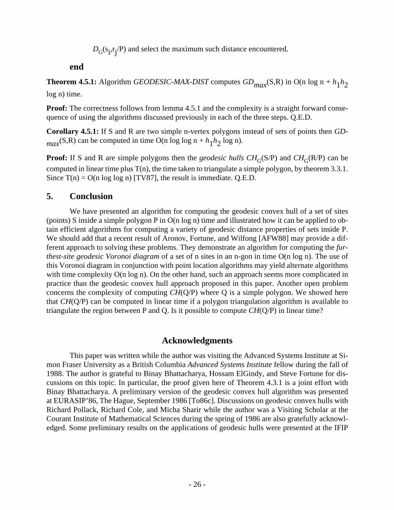
Theorem 4.5.1: Algorithm GEODESIC-MAX-DIST computesGDmax(S,R) in O(n log n +h1h2log n) time.

Proof: The correctness follows from lemma 4.5.1 and the complexity is a straight forward conse-quence of using the algorithms discussed previously in each of the three steps. Q.E.D.

Corollary 4.5.1: If S and R are two simple n-vertex polygons instead of sets of points thenGD-

max(S,R) can be computed in time O(n log log n +h1h2 log n).

Proof: If S and R are simple polygons then the geodesic hulls CHG(S/P) andCHG(R/P) can be

computed in linear time plus T(n), the time taken to triangulate a simple polygon, by theorem 3.3.1.Since T(n) = O(n log log n) [TV87], the result is immediate. Q.E.D.

5. Conclusion

We have presented an algorithm for computing the geodesic convex hull of a set of sites(points) S inside a simple polygon P in O(n log n) time and illustrated how it can be applied to ob-tain efficient algorithms for computing a variety of geodesic distance properties of sets inside P.We should add that a recent result of Aronov, Fortune, and Wilfong [AFW88] may provide a dif-ferent approach to solving these problems. They demonstrate an algorithm for computing thefur-thest-site geodesic Voronoi diagram of a set of n sites in an n-gon in time O(n log n). The use ofthis Voronoi diagram in conjunction with point location algorithms may yield alternate algorithmswith time complexity O(n log n). On the other hand, such an approach seems more complicated inpractice than the geodesic convex hull approach proposed in this paper. Another open problemconcerns the complexity of computingCH(Q/P) where Q is a simple polygon. We showed herethatCH(Q/P) can be computed in linear time if a polygon triangulation algorithm is available totriangulate the region between P and Q. Is it possible to computeCH(Q/P) in linear time?

Acknowledgments

This paper was written while the author was visiting the Advanced Systems Institute at Si-mon Fraser University as a British ColumbiaAdvanced Systems Institute fellow during the fall of1988. The author is grateful to Binay Bhattacharya, Hossam ElGindy, and Steve Fortune for dis-cussions on this topic. In particular, the proof given here of Theorem 4.3.1 is a joint effort withBinay Bhattacharya. A preliminary version of the geodesic convex hull algorithm was presentedat EURASIP’86, The Hague, September 1986 [To86c]. Discussions on geodesic convex hulls withRichard Pollack, Richard Cole, and Micha Sharir while the author was a Visiting Scholar at theCourant Institute of Mathematical Sciences during the spring of 1986 are also gratefully acknowl-edged. Some preliminary results on the applications of geodesic hulls were presented at the IFIP

- 25 -

can be computed in O(log n) time.

Step 3: For each site si in S compute h query geodesic distances DG(si,y/P) where y varies

over all convex vertices of CHG(S/P), for each si maximizing over y and finally

minimizing over i.

end

Using the algorithm of Guibas and Hershberger [GH87] in step 2 it is clear that the com-plexity of this algorithm is dominated by step 3. Therefore we have the following result.

Theorem 4.4.2: Algorithm GEODESIC-MEDIAN-2 computes the geodesic median of a set S in apolygon P in O(nh log n) time.

4.5 The maximum geodesic distance between two sets in P

In this section we consider the problem of computing the maximum geodesic distance be-tween two sets of sites in P. Accordingly, let S = s1, s2,...,sn and R = r1, r2,...,rn be the two

sets, each of cardinality n. Note that it is not important that S= R but this simplifies the com-plexity expressions.

Definition: The maximum geodesic distance between S and R in P, denoted by GDmax(S,R), is

the maximal geodesic distance between an element of S and an element of R, i.e.,

GDmax(S,R) = max max DG(si,rj/P)

i j

where i,j = 1,2,...,n.

Lemma 4.5.1: GDmax(S,R) is determined by a pair of elements si, rj such that si is a convex vertex

of CHG(S/P) and rj is a convex vertex of CHG(R/P).

This lemma immediately suggests the following algorithm for computing GDmax(S,R).

Algorithm GEODESIC-MAX-DIST

Input: A simple polygon P and two sets of sites S and R lying in P.

Output: The geodesic maximum distance between S and R, GDmax(S,R).

begin

Step 1: Compute the geodesic hulls CHG(S/P) and CHG(R/P).

Step 2: Preprocess P so that given two query points x,y in P the geodesic path between themcan be computed in O(log n) time.

Step 3: For every pair of sites si in S and rj in R such that they are convex vertices of their

respective geodesic hulls compute h1h2 geodesic distance queries of the form

- 24 -

us to improve on the brute-force algorithm in two different ways.

Lemma 4.4.1: The geodesic median of S in P is determined by a pair of sites in S one of whichmust be a convex vertex of CHG(S/P).

Algorithm GEODESIC-MEDIAN-1

Input: A simple polygon P and a set of points S lying in P.

Output: The geodesic median of S, MG(S/P).

begin

Step 1: Compute CHG(S/P).

Step 2: Triangulate CHG(S/P) to obtain T(CHG(S/P)).

Step 3: Preprocess T(CHG(S/P)) using O(n) space and O(n log n) time to support O(log n)-

time point-location queries.

Step 4: Determine for each triangle in T(CHG(S/P)) which points of S it contains.

Step 5: For each site si in S compute SPT(si,CHG(S/P)), record the furthest neighbor of siencountered and the accompanying distance, and identify the sites that minimizethis distance over all the sites si.

end

Each of the first four steps can be done in O(n log n) time with the procedures discussedearlier in the paper. In step 5, we have a triangulation of P available and thus we can computeSPT(si,CHG(S/P)) in O(n) time for each site using the algorithms in [El85] and [GHLST]. We have

thus established the following theorem.

Theorem 4.4.1: Algorithm GEODESIC-MEDIAN-1 computes the geodesic median of a set S in a

polygon P in O(n2) time.

We may also follow a different route to obtain an adaptive algorithm as follows.

Algorithm GEODESIC-MEDIAN-2

begin

Step 1: Compute CHG(S/P) and identify its h convex vertices.

Step 2: Preprocess P so that given two query points x,y in P the geodesic path between them

- 23 -

is denoted by RG(S/S). More precisely, for any site si in P define the covering radius of S from si as:

Cr(S/si) = max dG(si,y),

y

where y varies over all sites in S. Then the geodesic median of S is a site in S for which

RG(S/S) = min Cr(S/si),

si

where si varies over all sites in S.

It is clear that we can compute the geodesic median in O(n3) time using sheer brute forceif P is triangulated first. Before we present two more efficient algorithms for computing MG(S/P)

we introduce some more notation, a definition and a lemma.

Definition: The shortest path tree of a polygon P (with respect to a point x), denoted by SPT(x,P),is the union of GP(x,v/P) over all vertices v of P.

It is easily shown that SPT(x,P) is a planar tree rooted at x. This tree has n nodes, namelythe vertices of P, and its edges are straight segments connecting these nodes. It has been shown byElGindy [El85], and later independently in [GHLST] for a more restricted case, that given a mono-tone subdivision of P this tree can be computed in linear time. It follows from the fact that the fur-thest geodesic point in P from x must be a vertex of P that it can be computed in linear time ifSPT(x,P) is given. The following lemma, which follows directly from the previous results, allows

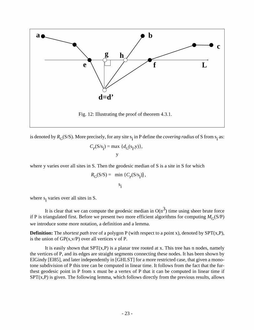
Fig. 12: Illustrating the proof of theorem 4.3.1.

a b

c

d=d’

e f L

g h

- 22 -

arise depending on whether (i) g lies behind e, (ii) g lies between e and f, or (iii) g lies ahead of f,on L. Consider first sub-case (ii). From Pythagoras’ theorem we may conclude that (1) GP(d,a/P)is longer than GP(g,e/P)∪ GP(e,a/P), (2) GP(d,c/P) is longer than GP(g,f/P)∪ GP(f,c/P), and (3)GP(d,b/P) is longer than GP(g,h/P)∪ GP(h,b/P). Therefore in this sub-case g is a better locationfor the geodesic center than is d, a contradiction. Similar arguments establish that in sub-case (i)vertex e is a better location for the geodesic center whereas vertex f is better for sub-case (iii).

Cases 2.2 and 2.3: CG(S/P) lies in aside or anend pocket. The proof for these two cases is similar

to that for the previous case. However, it may not be possible in this case to traverse vertices e andf (see Fig. 12) by a line L that does not intersect the interior of the geodesic triangle PG[a,b,c]. How-

ever if PG[a,b,c] intersects the interior of∆def we can construct a new triangle∆de’f’ such that e’f’

is parallel to ef and PG[a,b,c] does not intersect the interior of∆de’f’, by constructing e’f’ through

that vertex of PG[a,b,c] lying in∆def that maximizes the perpendicular distance to L in the direc-

tion of d. The arguments ofCase 2.1.2 can then be applied to∆de’f’ to complete the proof.

We have therefore proved thatCG(S/P) lies inCHG(S/P). It follows that all paths from

CG(S/P) to the convex vertices ofCHG(S/P) also lie inCHG(S/P) and those regions in P exterior to

CHG(S/P) may be disregarded. Q.E.D.

Theorem 4.3.1 suggests the following algorithm for computing the geodesic center of S.

Algorithm GEODESIC-CENTER

Input: A simple polygon P and a set of points S lying in P.

Output: The geodesic center of S,CG(S/P).

begin

Step 1: ComputeCHG(S/P) in O(n log n) time using the algorithm of section 3.

Step 2: ComputeCG(CHG(S/P)) in O(n log n) time using the algorithm of Pollack, Sharir,

and Rote [PSR88].

end

We have thus established the following theorem.

Theorem 4.3.2: Algorithm GEODESIC-CENTER computes the geodesic center of a set S in apolygon P in O(n log n) time.

4.4 The geodesic median of S in P

Definition: Thegeodesic median of S in P, denoted byMG(S/P), is the site in S, not necessarily

unique, whose maximal geodesic distance to any other site is the smallest possible. Such a distance

- 21 -

arise depending on whether or not d equals d’.

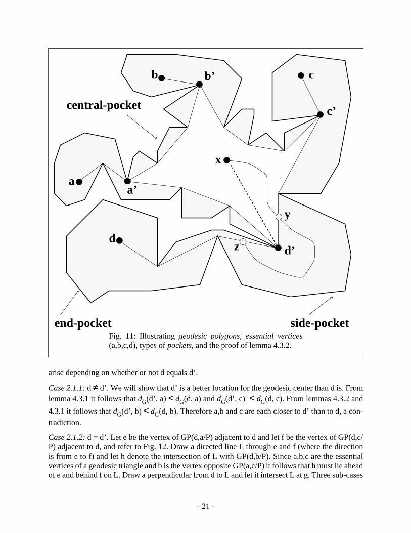
Case 2.1.1: d ≠ d’. We will show that d’ is a better location for the geodesic center than d is. Fromlemma 4.3.1 it follows that dG(d’, a) < dG(d, a) and dG(d’, c) < dG(d, c). From lemmas 4.3.2 and

4.3.1 it follows that dG(d’, b) < dG(d, b). Therefore a,b and c are each closer to d’ than to d, a con-

tradiction.

Case 2.1.2: d = d’. Let e be the vertex of GP(d,a/P) adjacent to d and let f be the vertex of GP(d,c/P) adjacent to d, and refer to Fig. 12. Draw a directed line L through e and f (where the directionis from e to f) and let h denote the intersection of L with GP(d,b/P). Since a,b,c are the essentialvertices of a geodesic triangle and b is the vertex opposite GP(a,c/P) it follows that h must lie aheadof e and behind f on L. Draw a perpendicular from d to L and let it intersect L at g. Three sub-cases

Fig. 11: Illustrating geodesic polygons, essential vertices(a,b,c,d), types of pockets, and the proof of lemma 4.3.2.

aa’

b b’ c

c’

dd’

x

y

z

end-pocket side-pocket

central-pocket

- 20 -

the interior of either a central pocket, a side pocket, or an end pocket of PG. In the first case it im-

plies GP(x,d/P) traverses the exterior of P, a contradiction. Therefore let GP(x,d/P) traverse a sidepocket of PG. It follows that GP(x,d/P) must properly intersect the interior of some edge of PG that

bounds the side pocket in question. Let y be such a point at which GP(x,d/P) enters the side pocket.Let z be the point on another edge of PG where GP(x,d/P) leaves the pocket. If GP(x,d/P) does not

leave the pocket then we have that z=d which is an instance of case three. In either situation, letp(y,z) denote the portion of PG from y to z and let q(y,z) denote the portion of GP(x,d/P) from y to

z. From lemma 4.3.1 it follows that both p(y,z) and q(y,z) are geodesic paths between y and z,which contradicts the uniqueness property of geodesics. The argument for the case when GP(x,d/P) enters an end pocket is similar. Q.E.D.

Theorem 4.3.1: The geodesic center of S in P is equal to the geodesic center of the geodesic con-vex hull of S, i.e., CG(S/P) = CG(CHG(S/P)).

Proof: The geodesic center of a finite set is determined by either two or three points of the set[AT85]. From lemma 4.2.1 it follows that given a set S in P, the geodesic furthest site in S fromany point x in P must be a convex vertex of CHG(S/P). Therefore CG(S/P) is determined by either

two or three convex vertices of CHG(S/P). On the other hand the geodesic center of a polygon Q is

determined by two or three convex vertices of Q. Therefore CG(CHG(S/P)) is determined by either

two or three convex vertices of CHG(S/P). This establishes that we need only consider those sites

in S that are convex vertices of CHG(S/P) in computing CG(S/P). Next we prove that CG(S/P) lies

in CHG(S/P) and that the regions of P that lie in the exterior of CHG(S/P) can be totally disregarded

in computing CG(S/P).

Case 1: The geodesic center is determined by two sites in S. In this case the geodesic center is themid-point of the geodesic diameter of S [AT85]. By lemma 4.2.1 the geodesic path realizing thegeodesic diameter of S must lie in CHG(S/P) and therefore so must the geodesic center of S.

Case 2: The geodesic center is determined by three sites in S. Let a,b,c ∈ S be the three sites thatdetermine the geodesic center of S and consider the geodesic triangle PG[a,b,c]. Since PG[a,b,c] is

also the geodesic convex hull of a,b,c it follows, by definition, that PG[a,b,c] ⊆ CHG(S/P). We will

show that the geodesic center of S must lie in PG[a,b,c]. Therefore let us assume the contrary. Three

cases arise depending on whether CG(S/P) lies in a central pocket, a side pocket, or an end pocket.

We assume that at least one of these pockets exists. If it does not it implies that S is “far” from theboundary of P and the shortest paths between the essential vertices of PG are actually single line

segments and PG is a Euclidean triangle. In this special case the geodesic center is equivalent to the

ordinary center in the classical Euclidean facility location problem and it is well known that thiscenter must lie in such a triangle [CR47].

Case 2.1: CG(S/P) lies in a central pocket. Let d denote the location of CG(S/P) in a central pocket

determined, without loss of generality, by endpoints lying in GP(a’,c’/P). Construct GP(d,a/P) andGP(d,c/P) and let d’ be the point such that GP(d,a/P) ∩ GP(d,c/P) = GP(d,d’/P). Two sub-cases

- 19 -

the covering radius of S from x as:

Cr(S/x) = max dG(x,y),

y

where y varies over all sites in S. Then the geodesic center of S is the point in P for which

RG(S/P) = min Cr(S/x) ,

x

where x varies over all points in P.

The following lemmas and theorem allow us to solve this problem efficiently.

Lemma 4.3.1: Let x’ and y’ be two points on a geodesic path GP(x,y/P) such that x’ is the closerto x on GP(x,y/P). Then GP(x’,y’/P) is contained in GP(x,y/P).

Proof: Assume the contrary and let p(x’,y’) denote the portion of GP(x,y/P) between x’ and y’.Since geodesic paths are unique it follows that the length of GP(x’,y’/P) is less than the length ofp(x’,y’). Therefore we may construct a path GP(x,x’/P) ∪ GP(x’,y’/P) ∪ GP(y’,y/P) which isshorter than GP(x,y/P), a contradiction. Q.E.D.

Given m points p1,p2,...,pm in P we may connect pi to pi+1 for i=1,2,...,m (modulo m) with

GP(pi, pi+1/P) to obtain a polygonal circuit. If this polygonal circuit is a weakly-simple polygon

then we say it is a geodesic m-gon or polygon and denote it by PG[p1,p2,...,pm] or PG for short

when the context is clear. The m vertices p1,p2,...,pm of PG form its essential vertices. The remain-

ing vertices of PG coincide with reflex vertices of P. If m=3 we obtain a geodesic triangle, and so

on. Fig. 11 illustrates a geodesic quadrilateral PG[a,b,c,d]. For a geodesic polygon

PG[p1,p2,...,pm] there exist vertices p’1,p’2,...,p’m (pi and p’i need not be distinct for any value of

i) such that the paths GP(pi, pi+1/P) and GP(pi, pi-1/P) intersect in GP(pi, p’i/P) for all values of

i. If the boundary of PG intersects the boundary of P then these intersection points decompose the

boundary of P into polygonal chains that do not intersect the boundary of PG other that at their end-

points. The regions bounded by these chains and the corresponding portions of bd(P) are calledpockets (see Fig. 11) and the chains are referred to as pocket chains. It is useful to distinguish be-tween three types of pockets. If a pocket chain has both its end-points in GP(p’i, p’i+1/P) for some

value of i then the pocket, the interior of which does not contain the interior of PG, is a central pock-

et. If a pocket contains at least one essential vertex of PG it is an end pocket. All other pockets are

called side pockets.

Lemma 4.3.2: Let PG[p1,p2,...,pm] be a geodesic polygon in P and assume that there exists an es-

sential vertex of PG, say pi=d, with corresponding p’i=d’, such that GP(pi, pi+1/P) and GP(pi, pi-

1/P) intersect in GP(pi, p’i/P). Let x be any point in PG. Then GP(x,d/P) must intersect d’.

Proof: (Refer to Fig. 11) Assume GP(x,d/P) does not intersect d’. Then GP(x,d/P) must traverse

- 18 -

have that GP(x,y’) < maxGP(x,b), GP(x,c). Therefore there must exist a convex vertex ofCHG(S/P), say c, such that GP(x,y) < GP(x,c) which is a contradiction. The same argument can

then be used to show that GP(c,x) is at most as long as GP(c,e) where e is also a convex vertex ofCHG(S/P) and the first result follows. Next we show that DG(S/P) = DG(CHG(S/P)). From the first

result it follows that DG(CHG(S/P)) is determined by two sites si and sj in S. Furthermore, by def-

inition the geodesic path in P between every pair of sites in S must lie in CHG(S/P). Therefore the

path realizing DG(S/P) must also be the path realizing DG(CHG(S/P)). Q.E.D.

This result then immediately suggests an adaptive version of the previous algorithm. Let hdenote the number of convex vertices of CHG(S/P). First compute CHG(S/P) and identify its con-

vex vertices in O(n log n) time with the algorithm described in the previous section. Then prepro-cess P with the algorithm of Guibas and Hershberger [GH87] to admit O(log n) time computationof geodesic distance queries between pairs of query sites. Finally answer the queries for all pairsof sites which are convex vertices of CHG(S/P) and select the maximum geodesic distance encoun-

tered. The time complexity of this algorithm is O(n log n + h2 log n). However, the most dramaticapplication of lemma 4.2.1 is obtained by using the fact that the geodesic diameter of a simple poly-gon can be computed in O(n log n) time [Su86a] as in the following algorithm.

Algorithm GEODESIC-DIAMETER

Input: A simple polygon P and a set of points S lying in P.

Output: The geodesic diameter of S, DG(S/P).

begin

Step 1: Compute CHG(S/P) using the algorithm discussed in the previous section.

Step 2: Compute DG(CHG(S/P)) using Suri’s algorithm [Su86a].

end

We have thus established the following theorem.

Theorem 4.2.1: Algorithm GEODESIC-DIAMETER computes the geodesic diameter of a set S ina simple polygon P in O(n log n) time.

4.3 The geodesic center of S in P

Definition: The geodesic center of a set of sites S in a simple polygon P, denoted by CG(S/P), is a

point in P which minimizes the maximum geodesic distance to any site in S. Such a distance iscalled the geodesic radius of S and denoted by RG(S/P). More precisely, for any point x in P define

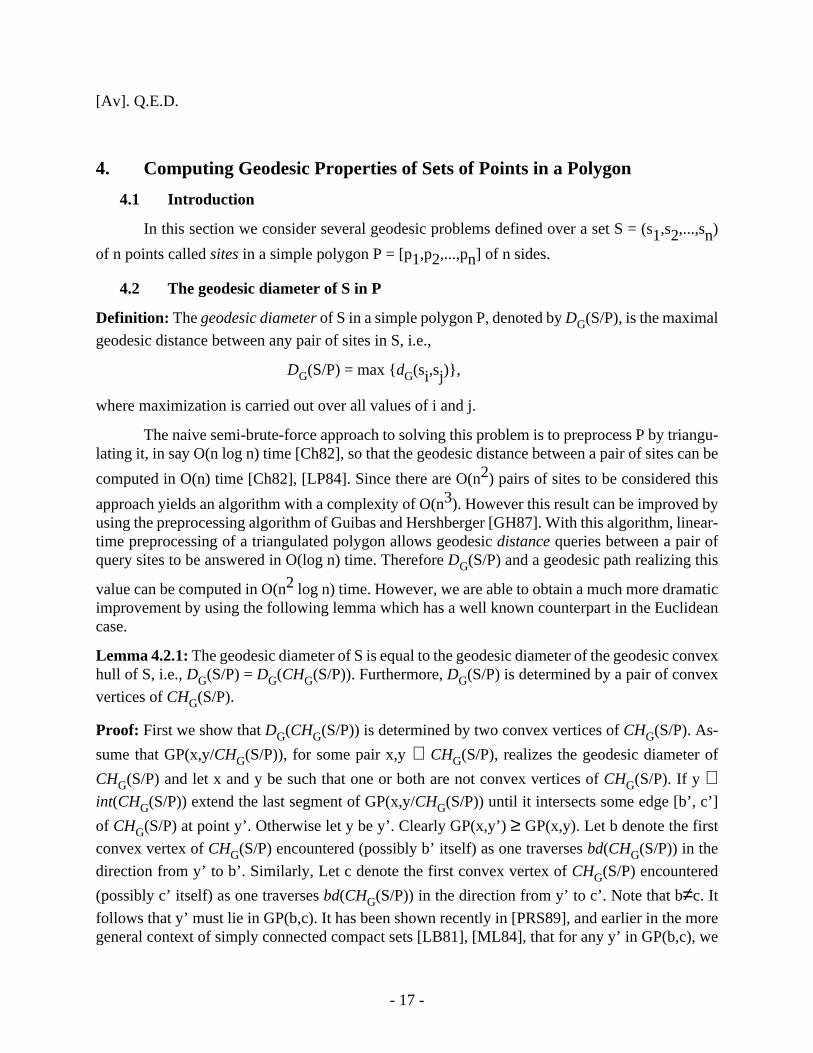
- 17 -

[Av]. Q.E.D.

4. Computing Geodesic Properties of Sets of Points in a Polygon

4.1 Introduction

In this section we consider several geodesic problems defined over a set S = (s1,s2,...,sn)

of n points called sites in a simple polygon P = [p1,p2,...,pn] of n sides.

4.2 The geodesic diameter of S in P

Definition: The geodesic diameter of S in a simple polygon P, denoted by DG(S/P), is the maximal

geodesic distance between any pair of sites in S, i.e.,

DG(S/P) = max dG(si,sj),

where maximization is carried out over all values of i and j.

The naive semi-brute-force approach to solving this problem is to preprocess P by triangu-lating it, in say O(n log n) time [Ch82], so that the geodesic distance between a pair of sites can be

computed in O(n) time [Ch82], [LP84]. Since there are O(n2) pairs of sites to be considered this

approach yields an algorithm with a complexity of O(n3). However this result can be improved byusing the preprocessing algorithm of Guibas and Hershberger [GH87]. With this algorithm, linear-time preprocessing of a triangulated polygon allows geodesic distance queries between a pair ofquery sites to be answered in O(log n) time. Therefore DG(S/P) and a geodesic path realizing this

value can be computed in O(n2 log n) time. However, we are able to obtain a much more dramaticimprovement by using the following lemma which has a well known counterpart in the Euclideancase.

Lemma 4.2.1: The geodesic diameter of S is equal to the geodesic diameter of the geodesic convexhull of S, i.e., DG(S/P) = DG(CHG(S/P)). Furthermore, DG(S/P) is determined by a pair of convex

vertices of CHG(S/P).

Proof: First we show that DG(CHG(S/P)) is determined by two convex vertices of CHG(S/P). As-

sume that GP(x,y/CHG(S/P)), for some pair x,y ∈ CHG(S/P), realizes the geodesic diameter of

CHG(S/P) and let x and y be such that one or both are not convex vertices of CHG(S/P). If y ∈int(CHG(S/P)) extend the last segment of GP(x,y/CHG(S/P)) until it intersects some edge [b’, c’]

of CHG(S/P) at point y’. Otherwise let y be y’. Clearly GP(x,y’) ≥ GP(x,y). Let b denote the first

convex vertex of CHG(S/P) encountered (possibly b’ itself) as one traverses bd(CHG(S/P)) in the

direction from y’ to b’. Similarly, Let c denote the first convex vertex of CHG(S/P) encountered

(possibly c’ itself) as one traverses bd(CHG(S/P)) in the direction from y’ to c’. Note that b≠c. It

follows that y’ must lie in GP(b,c). It has been shown recently in [PRS89], and earlier in the moregeneral context of simply connected compact sets [LB81], [ML84], that for any y’ in GP(b,c), we

- 16 -

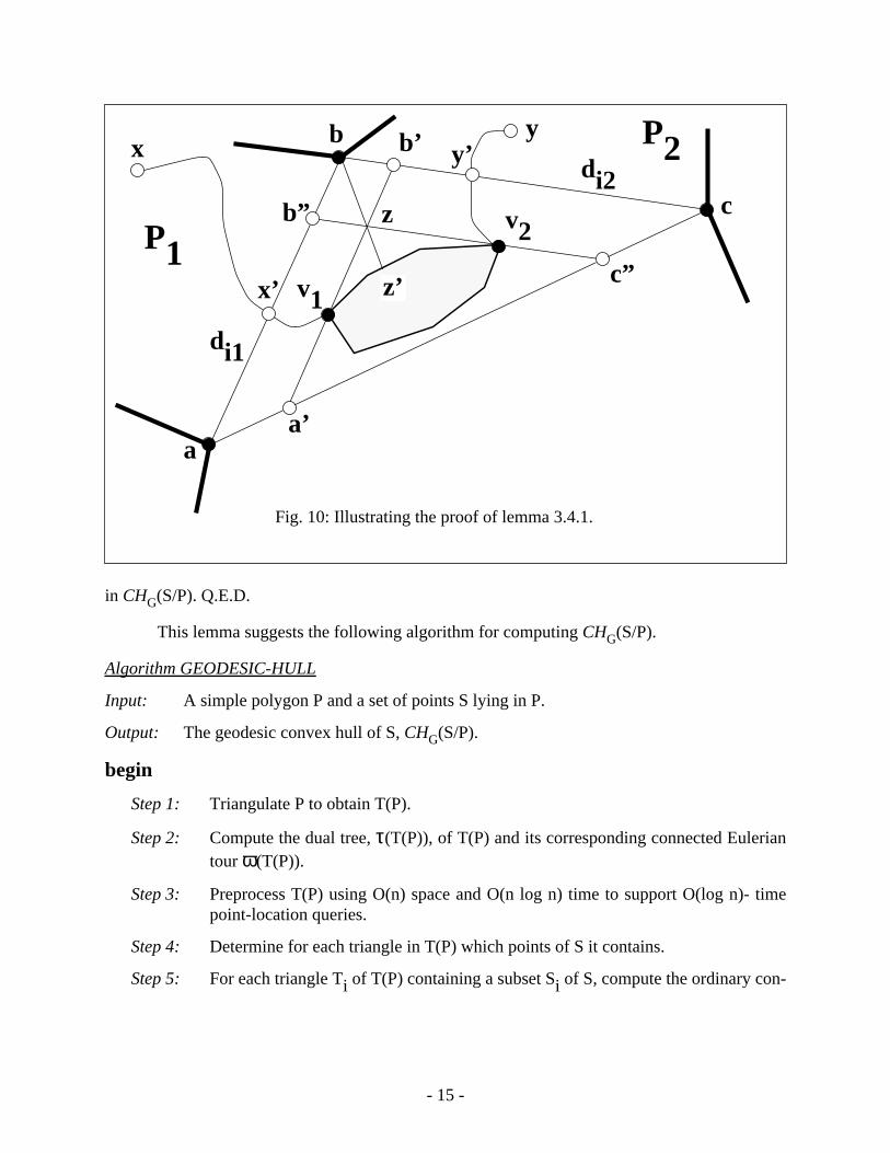
vex hull CH(Si).

Step 6: For each set Si lying in Ti compute all the connecting vertices.

Step 7: Perform a counterclockwise scan of ω(T(P)) and compute the geodesic paths be-tween consecutive connecting vertices in the order in which they are encountered.

Step 8: Concatenate the geodesic paths computed in Step 7 with the appropriate sub-chainsof the CH(Si), for all i, to yield the weakly-simple polygon Q*.

Step 9: Triangulate A(P-Q*).

Step 10: Compute CHG(S/P) = CHG(A(P-Q*)/P).

end

Theorem 3.4.1: Algorithm GEODESIC-HULL computes the geodesic convex hull of a set of npoints in a simple polygon of n sides in Ο(n log n) time using O(n) space.

Proof: The correctness follows from the previous lemmas and the correctness of the algorithmsused. We turn thus to the complexity. Step 1 can be done in O(n log log n) time [TV88]. Step 2 canbe done in linear time [PS85]. Steps 3 and 4 can be accomplished using the algorithm of Kirk-patrick [Ki83]. In step 5 the convex hulls in all triangles of T(P) containing points of S can be com-puted with a variety of existing algorithms [To85] in a total time of O(n log n). Step 6 can be donein O(ni) time for each triangle Ti containing points of S, where ni is the number of vertices of

CH(Si), by a simple scan of bd(CH(Si)) while keeping track of the minimum perpendicular dis-

tance to the relevant diagonal encountered. Since there are at most a constant number of connectingvertices for each triangle in T(P) and since Σ ni over all i is O(n) it follows that the total time for

step 6 is O(n). Step 7 consists of computing a sequence of geodesic paths corresponding to a se-quence of sleeves the total length of which is at most 2n. This is a direct consequence of the factthat the length of ω(T(P)) is at most twice the length of τ(T(P)). Since in each such sleeve of sizen* the geodesic path required can be computed in time O(n*) using the algorithms in [Ch82] and[LP84] it follows that step 7 can be performed in a total time of O(n). Step 8 consists of a meretraversal of all the boundaries of the CH(Si) and therefore runs in O(n) time in the worst case. In

step 9 A(P-Q*) can be converted to a weakly simple polygon in O(n) time and then triangulated inO(n log log n) time as in step 1. Step 10 is an instance of the problem discussed in the previoussection and can be accomplished in O(n) time. All the steps require no more than linear storagespace. We therefore conclude that the space requirement for the algorithm is linear and the time isdominated by steps 3 and 4 and is thus O(n log n). Finally we remark that Ω(n log n) is a lowerbound on the time complexity of this problem. This follows from the fact that if P is convex thenCHG(S/P) = CH(S) and it is well known that Ω(n log n) is a lower bound for computing CH(S)

- 15 -

in CHG(S/P). Q.E.D.

This lemma suggests the following algorithm for computing CHG(S/P).

Algorithm GEODESIC-HULL

Input: A simple polygon P and a set of points S lying in P.

Output: The geodesic convex hull of S, CHG(S/P).

begin

Step 1: Triangulate P to obtain T(P).

Step 2: Compute the dual tree, τ(T(P)), of T(P) and its corresponding connected Euleriantour ω(T(P)).

Step 3: Preprocess T(P) using O(n) space and O(n log n) time to support O(log n)- timepoint-location queries.

Step 4: Determine for each triangle in T(P) which points of S it contains.

Step 5: For each triangle Ti of T(P) containing a subset Si of S, compute the ordinary con-

Fig. 10: Illustrating the proof of lemma 3.4.1.

a

b

c

di1

di2

a’

b’

b”

c”

z

z’v1

v2P1

P2x

x’

yy’

- 14 -

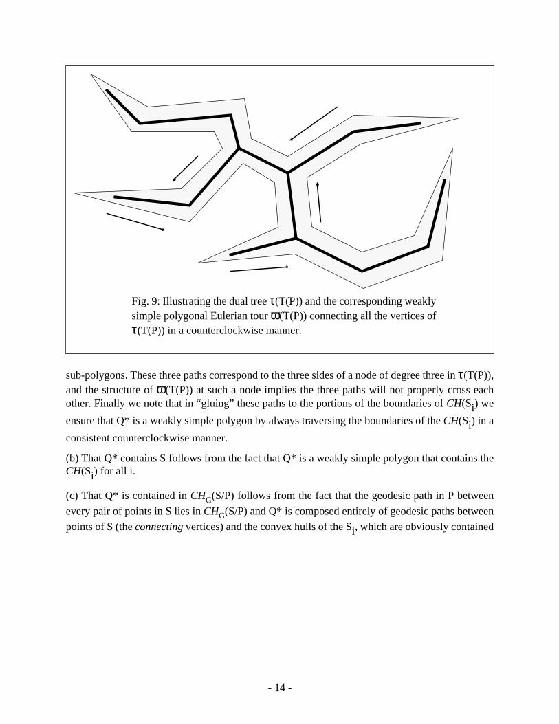
sub-polygons. These three paths correspond to the three sides of a node of degree three in τ(T(P)),and the structure of ω(T(P)) at such a node implies the three paths will not properly cross eachother. Finally we note that in “gluing” these paths to the portions of the boundaries of CH(Si) we

ensure that Q* is a weakly simple polygon by always traversing the boundaries of the CH(Si) in a

consistent counterclockwise manner.

(b) That Q* contains S follows from the fact that Q* is a weakly simple polygon that contains theCH(Si) for all i.

(c) That Q* is contained in CHG(S/P) follows from the fact that the geodesic path in P between

every pair of points in S lies in CHG(S/P) and Q* is composed entirely of geodesic paths between

points of S (the connecting vertices) and the convex hulls of the Si, which are obviously contained

Fig. 9: Illustrating the dual tree τ(T(P)) and the corresponding weaklysimple polygonal Eulerian tour ω(T(P)) connecting all the vertices ofτ(T(P)) in a counterclockwise manner.

- 13 -

[b",c"] intersect at z and let the ray emanating at b through z intersect bd(CH(Si)) at z’. By con-

struction z’ must lie after v2 and before v1 in clockwise order. Therefore [v1,x’] must lie in quad-

rilateral [a,a’,z,b] and [v2,y’] must lie in quadrilateral [c,b,z,c"]. Since the interiors of these two

quadrilaterals do not intersect it implies that GP(v1,x/P) and GP(v2,y/P) do not properly cross each

other in Ti.

Consider now any triangle Tk that is empty of points in S. Two cases arise: (i) Tk contains

two diagonals of T(P) which are not edges of P and (ii) Tk contains three diagonals of T(P) which

are not edges of P. Note that if Tk contains only one diagonal of T(P) not an edge in P and Tk does

not contain any points of S then no geodesic paths traverse Tk. Case (i): Tk cuts off two sub-poly-

gons of P, P1 and P2. If P1 or P2 contain no points of S then the geodesic paths do not traverse Tk.

If both P1 and P2 contain points of S then the geodesic paths correspond to both sides of a chain

in τ(T(P)) and therefore they do not properly cross each other. Case (ii): Tk cuts off three sub-poly-

gons of P, P1, P2 and P3. If only one of these contains points of S then the geodesic paths do not

traverse Tk. If two sub-polygons contain points of S then we have a situation identical to case (i).

If all three contain subsets of S then three geodesic paths will traverse Tk between every pair of

Fig. 8: Illustrating the connecting vertices (marked solid black) of theconvex hull of the subset of S lying in triangle Ti.

CH(Si)

dikvik

Ti

- 12 -

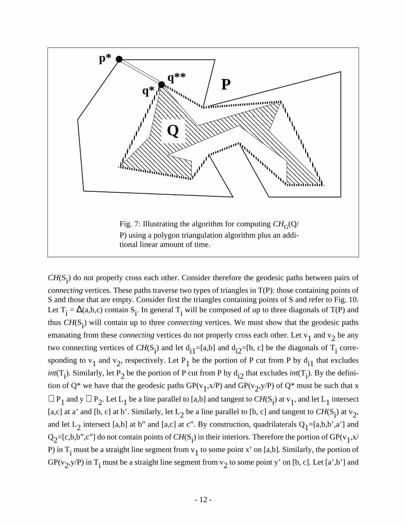
CH(Si) do not properly cross each other. Consider therefore the geodesic paths between pairs of

connecting vertices. These paths traverse two types of triangles in T(P): those containing points ofS and those that are empty. Consider first the triangles containing points of S and refer to Fig. 10.Let Ti = ∆(a,b,c) contain Si. In general Ti will be composed of up to three diagonals of T(P) and

thus CH(Si) will contain up to three connecting vertices. We must show that the geodesic paths

emanating from these connecting vertices do not properly cross each other. Let v1 and v2 be any

two connecting vertices of CH(Si) and let di1=[a,b] and di2=[b, c] be the diagonals of Ti corre-

sponding to v1 and v2, respectively. Let P1 be the portion of P cut from P by di1 that excludes

int(Ti). Similarly, let P2 be the portion of P cut from P by di2 that excludes int(Ti). By the defini-

tion of Q* we have that the geodesic paths GP(v1,x/P) and GP(v2,y/P) of Q* must be such that x

∈ P1 and y ∈ P2. Let L1 be a line parallel to [a,b] and tangent to CH(Si) at v1, and let L1 intersect

[a,c] at a’ and [b, c] at b’. Similarly, let L2 be a line parallel to [b, c] and tangent to CH(Si) at v2,

and let L2 intersect [a,b] at b” and [a,c] at c”. By construction, quadrilaterals Q1=[a,b,b’,a’] and

Q2=[c,b,b”,c”] do not contain points of CH(Si) in their interiors. Therefore the portion of GP(v1,x/

P) in Ti must be a straight line segment from v1 to some point x’ on [a,b]. Similarly, the portion of

GP(v2,y/P) in Ti must be a straight line segment from v2 to some point y’ on [b, c]. Let [a’,b’] and

Fig. 7: Illustrating the algorithm for computing CHG(Q/

P) using a polygon triangulation algorithm plus an addi-tional linear amount of time.

Q

P

p*

q*q**

- 11 -

using two copies of each such geodesic path in a judicious manner, we obtain a polygon Q*. By ajudicious manner it is meant that in constructing a description of the boundary of Q* the directionsof the geodesic paths and portions of the boundaries of the CH(Si), for all i, must be properly cho-

sen. To do this we begin by doubling each edge of τ(T(P)), thereby obtaining a graph ω(T(P)), eachvertex of which has even degree and which therefore is a connected Euler graph, i.e., its edges canbe numbered so that the resulting sequence is a weakly-simple polygon oriented in a counterclock-wise manner (see Fig. 9). A geodesic path between two connecting vertices in T(P) is contained inthose triangles determined by the portion of ω(T(P)) corresponding to the relevant portion of thedual tree. The relative position and direction of the portion of ω(T(P)) determines the relative po-sition and direction of its corresponding geodesic path. Finally we need to append correctly theportions of the boundaries of the CH(Si) between connecting vertices. A connecting vertex, say

v(i,k), in a triangle Ti is connected to the first connecting vertex encountered (possibly v(i,k) itself)

in traversing the boundary of CH(Si) in a counter-clockwise manner. Furthermore, the connection

is made by appending precisely the polygonal chain traversed during this search with a directionidentical to the direction in which the search is made. We will now show that Q* does indeed pos-sess the desired properties mentioned above.

Lemma 3.4.1: The polygon Q* has the following properties: (a) Q* is weakly-simple, (b) Q* con-tains S, (c) Q* is contained in CHG(S/P).

Proof: (a) Since the sets Si are contained in disjoint triangles it follows that the boundaries of the

Fig. 6: The shaded region in P is the geodesic convexhull of the set of points in P.

P

- 10 -

CH(Sj) and appending the geodesic paths between appropriate connecting vertices computed with-

in an appropriate sleeve of P. Consider CH(Si) lying in Ti and refer to Fig. 8. A triangle Ti contains

either one, two, or three diagonals of T(P) depending on whether it shares two, one, or zero edgesof P, respectively. Each diagonal of Ti is associated with a connecting vertex of CH(Si). The con-

necting vertex of CH(Si) corresponding to diagonal dik of Ti is that vertex, say v(i,k), of CH(Si)

which is closest, in the perpendicular distance sense, to the line collinear with dik. Note that a sin-

gle vertex of CH(Si) may be a connecting vertex for more than one diagonal of Ti. Let Ti and Tjbe two triangles in T(P) such that each contains points Si and Sj, respectively. Let ti and tj denote

the nodes in τ(T(P)) corresponding to Ti and Tj, respectively. The shortest path (in the graph-the-

oretic sense) between ti and tj in τ(T(P)) corresponds to a sleeve in T(P) denoted by Sl(Ti,...,Tj).

This sleeve Sl(Ti,...,Tj) specifies a sequence of ordered diagonals dik,...,djm that must be intersect-

ed sequentially by the geodesic path between any point x ∈ int(Ti) and any point y ∈ int(Tj). Let

v(i,k) and v(j,m) denote the connecting vertices of CH(Si) and CH(Sj), respectively, corresponding

to diagonals dij and dkm in Ti and Tj. The connecting vertices v(i,k) and v(j,m) are joined by the

geodesic path between them provided that no points of S lie in any triangle of Sl(Ti,...,Tj) other

than Ti and Tj. By applying this rule to all pairs of triangles in T(P) that contain points of S and

Fig 5: (a) The shaded subset of P is not geodesically convex because eventhough x,y ∈ Q, we have that GP(x,y/P) ≠ GP(x,y/Q). (b) The shaded sub-set of P is geodesically convex.

(a) (b)

xy

P P

Q

Q

- 9 -

following theorem.

Theorem 3.3.1: Given two simple polygons P = [p1,p2,...,pn] and Q=[q1,q2,...,qn] such that Q is

contained in P, CHG(Q/P) can be computed using a polygon triangulation algorithm and O(n) ad-

ditional time.

3.4 Computing the geodesic convex hull of a set of points in a polygon

In this section we present Algorithm GEODESIC-HULL for computing CHG(S/P) in O(n

log n) time which is optimal to within a constant factor. The essential idea used to solve this prob-lem is to convert the problem, in O(n log n) time, to an instance of the CHG(Q/P) problem. In other

words, we first find a weakly simple polygon Q* that has the properties that: (1) Q* lies in P, (2)Q* contains S, and (3) CHG(Q*/P) = CHG(S/P). Before presenting the algorithm we provide a suit-

able definition of the polygon Q* and establish that it possesses the desired properties.

A triangulation T(P) of P contains n-2 triangles denoted by Ti, i=1,2,...,n-2. Let the dual

tree of T(P) be denoted by τ(T(P)). Let the subset of sites in S that fall in triangle Ti be denoted by

Si and let CH(Si) denote the ordinary convex hull of Si. The weakly simple polygon Q* is com-

posed of the union of the CH(Si), i=1,2,...,n-2, with certain geodesic paths connecting them. Two

convex hulls CH(Si) and CH(Sj) are connected by specifying connecting vertices of CH(Si) and

Fig. 4: Illustrating a weakly-simple polygon P. The in-terior of P is shaded. The arrows indicate a counter-clockwise traversal of the boundary of P. Here somevertices and edges of P are used twice.

P

P

- 8 -

puted in linear time given that the region A(P-Q) is triangulated. We will show the more generalresult instead that given Q contained in P, CHG(Q/P) can be computed in O(n) time given that an

algorithm is available to triangulate a simple polygon. First we state two elementary lemmas with-out proof.

Lemma 3.3.1: Let q* be a vertex of CH(Q), the ordinary convex hull of Q. Then q* must be a ver-tex of CHG(Q/P).

Lemma 3.3.2: A vertex p* of P such that int[p*,q*] lies in int(P) ∩ ext(Q) can be found in O(n)time.

The above lemmas suggest the following approach. First we determine in linear time a ver-tex q* of CH(Q). This can be done by choosing any extreme vertex of Q in some arbitrarily spec-ified direction. Without loss of generality let q* be the vertex with maximum y-coordinate and re-fer to Fig. 7. Then by lemma 3.3.2 we find a vertex p* of P visible from q* also in linear time. Theline segment [p*,q*] partitions the non-simple region A(P-Q) into a simple region and by insertingtwo copies of [p*,q*] into the descriptions of the boundaries of P and Q we convert the non-simpleregion A(P-Q) into a weakly simple polygon P*. This polygon P* can now be triangulated in O(nlog log n) time [TV87] thus affording the computation of the geodesic path between two points x,yin P* in linear time [Ch82], [LP84]. From lemma 3.3.1 it follows that CHG(Q/P) is the shortest path

in P* between q* and q**, a copy of q* lying on the other side of [p*,q*]. Furthermore q* and q**are two points in the triangulated weakly simple polygon P*. Therefore we have established the

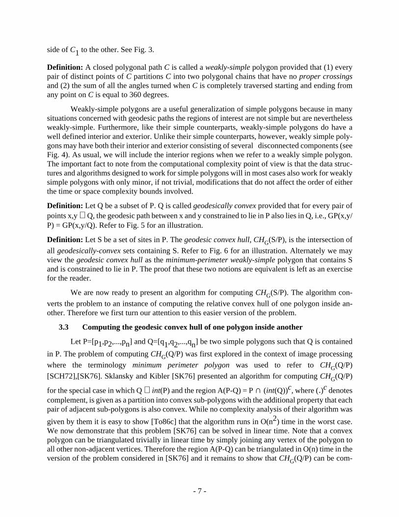
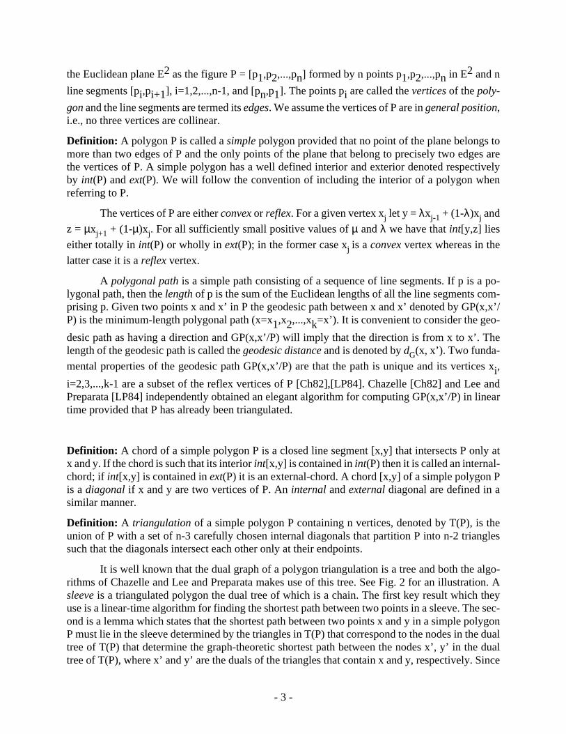
Fig. 3: Illustrating intersecting curves (a) with propercrossings and (b) without proper crossings.

(a) (b)

C1

C1

C1

C1

C1

C1

C2

C2

C2

C2 C2

- 7 -

side of C1 to the other. See Fig. 3.

Definition: A closed polygonal path C is called a weakly-simple polygon provided that (1) everypair of distinct points of C partitions C into two polygonal chains that have no proper crossingsand (2) the sum of all the angles turned when C is completely traversed starting and ending fromany point on C is equal to 360 degrees.

Weakly-simple polygons are a useful generalization of simple polygons because in manysituations concerned with geodesic paths the regions of interest are not simple but are neverthelessweakly-simple. Furthermore, like their simple counterparts, weakly-simple polygons do have awell defined interior and exterior. Unlike their simple counterparts, however, weakly simple poly-gons may have both their interior and exterior consisting of several disconnected components (seeFig. 4). As usual, we will include the interior regions when we refer to a weakly simple polygon.The important fact to note from the computational complexity point of view is that the data struc-tures and algorithms designed to work for simple polygons will in most cases also work for weaklysimple polygons with only minor, if not trivial, modifications that do not affect the order of eitherthe time or space complexity bounds involved.

Definition: Let Q be a subset of P. Q is called geodesically convex provided that for every pair ofpoints x,y ∈ Q, the geodesic path between x and y constrained to lie in P also lies in Q, i.e., GP(x,y/P) = GP(x,y/Q). Refer to Fig. 5 for an illustration.

Definition: Let S be a set of sites in P. The geodesic convex hull, CHG(S/P), is the intersection of

all geodesically-convex sets containing S. Refer to Fig. 6 for an illustration. Alternately we mayview the geodesic convex hull as the minimum-perimeter weakly-simple polygon that contains Sand is constrained to lie in P. The proof that these two notions are equivalent is left as an exercisefor the reader.

We are now ready to present an algorithm for computing CHG(S/P). The algorithm con-

verts the problem to an instance of computing the relative convex hull of one polygon inside an-other. Therefore we first turn our attention to this easier version of the problem.

3.3 Computing the geodesic convex hull of one polygon inside another

Let P=[p1,p2,...,pn] and Q=[q1,q2,...,qn] be two simple polygons such that Q is contained

in P. The problem of computing CHG(Q/P) was first explored in the context of image processing

where the terminology minimum perimeter polygon was used to refer to CHG(Q/P)

[SCH72],[SK76]. Sklansky and Kibler [SK76] presented an algorithm for computing CHG(Q/P)

for the special case in which Q ⊂ int(P) and the region A(P-Q) = P ∩ (int(Q))c, where (.)c denotescomplement, is given as a partition into convex sub-polygons with the additional property that eachpair of adjacent sub-polygons is also convex. While no complexity analysis of their algorithm was

given by them it is easy to show [To86c] that the algorithm runs in O(n2) time in the worst case.We now demonstrate that this problem [SK76] can be solved in linear time. Note that a convexpolygon can be triangulated trivially in linear time by simply joining any vertex of the polygon toall other non-adjacent vertices. Therefore the region A(P-Q) can be triangulated in O(n) time in theversion of the problem considered in [SK76] and it remains to show that CHG(Q/P) can be com-

- 6 -

location problem asks for the location of a facility to be used by the customers such that the max-imum Euclidean distance that any customer has to travel to get to the facility is minimized. Thecenter of the minimal spanning circle of the sites, i.e., the smallest circle enclosing the sites, is thesolution to this problem.

Definition: The geodesic center of a simple polygon P, denoted by CG(P), is a point in P which

minimizes the maximum geodesic distance to any point in P. Such a distance is called the geodesicradius of P and denoted by RG(P). More precisely, for any point x in P define the covering radius

of P from x as:

Cr(P/x) = max dG(x,y),

y

where y varies over all points in P. Then the geodesic center of P is the point in P for which

RG(P) = min Cr(P/x),

x

where x varies over all points in P.

It is now well known that the standard Euclidean facility problem can be solved in lineartime [Me83], [Dy86], but its generalization to the geodesic metric appears to be more difficult. Theproblem of computing the geodesic center of a simple polygon was first investigated by Asano andToussaint [AT85] who showed that it was unique and could be computed in O(n4 log n) time. Thisresult was later improved to O(n3 log log n) time in [AT86], to O(n log2 n) time in [PS86], andfinally to O(n log n) time in [PSR89].

3. The Geodesic Convex Hull

3.1 Introduction

In this section we introduce the notion of the geodesic (also known in the literature as rel-ative) convex hull of a set of points S = s1,s2,...,sn called sites lying in a simple n-gon P. Note

that the cardinalities of S and P need not be equal but this assumption will simplify the complexityformulas. The geodesic convex hull of S given P, denoted by CHG(S/P), turns out to be a funda-

mental tool for computing many geodesic properties efficiently as will be demonstrated in section4.

3.2 Geometric preliminaries

Definition: Let C1 and C2 be two oriented, possibly self-intersecting curves. We say that C1 and

C2 have a proper crossing provided that, as we traverse C1 from its starting point to its finishing

point we encounter a neighbourhood of C1 where C2 intersects C1 and actually switches from one

- 5 -

of the set and since the convex hull of a simple polygon P can be found in O(n) time [MA79], itfollows that the diameter of P can be found in O(n) time also. The geodesic diameter consideredhere is a generalization of the Euclidean diameter.

Definition: The geodesic diameter of a simple polygon P, denoted by DG(P), is the maximal geo-

desic distance between any pair of points in P, i.e.,

DG(P) = max dG(x,y),

x,y

where x and y vary over all points of P.

Chazelle [Ch82] as well as Reif and Storer [RS85] give O(n2) time algorithms for comput-ing the geodesic diameter of a simple n-gon. It is known that a geodesic furthest neighbor of a pointin a polygon is always a convex vertex of P (see Asano and Toussaint [AT85]). This immediatelyleads to an algorithm with complexity O(c2n + T(n)) where c is the number of convex vertices ofP and T(n) is the time required to triangulate P. Suri [Su87] on the other hand has shown that O(nlog n) time is sufficient to compute the geodesic furthest neighbors of all the vertices of P and,hence, to compute the geodesic diameter of P.

2.3 The geodesic center of a polygon

The geodesic center of a polygon is a generalization of the Euclidean facility location prob-lem. Given a set of points in the plane called sites that represent customers, the Euclidean facility

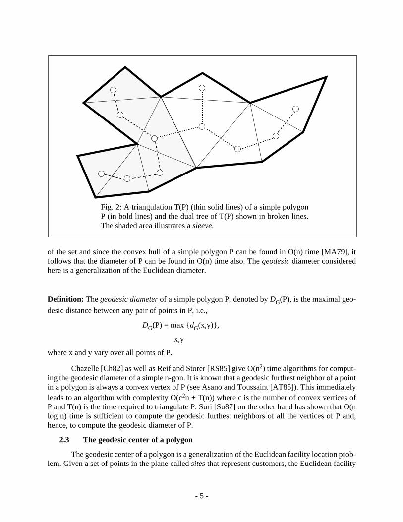
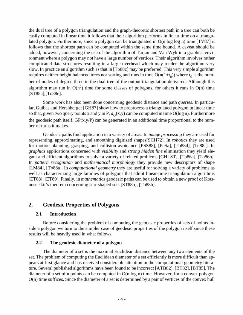
Fig. 2: A triangulation T(P) (thin solid lines) of a simple polygonP (in bold lines) and the dual tree of T(P) shown in broken lines.The shaded area illustrates a sleeve.

- 4 -

the dual tree of a polygon triangulation and the graph-theoretic shortest path in a tree can both beeasily computed in linear time it follows that their algorithm performs in linear time on a triangu-lated polygon. Furthermore, since a polygon can be triangulated in O(n log log n) time [TV87] itfollows that the shortest path can be computed within the same time bound. A caveat should beadded, however, concerning the use of the algorithm of Tarjan and Van Wyk in a graphics envi-ronment where a polygon may not have a large number of vertices. Their algorithm involves rathercomplicated data structures resulting in a large overhead which may render the algorithm veryslow. In practice an algorithm such as that in [To88c] may be preferred. This very simple algorithmrequires neither height balanced trees nor sorting and runs in time O(n(1+t0)) where t0 is the num-

ber of nodes of degree three in the dual tree of the output triangulation delivered. Although thisalgorithm may run in O(n2) time for some classes of polygons, for others it runs in O(n) time[ST88a],[To88e].

Some work has also been done concerning geodesic distance and path queries. In particu-lar, Guibas and Hershberger [GH87] show how to preprocess a triangulated polygon in linear timeso that, given two query points x and y in P, dG(x,y) can be computed in time O(log n). Furthermore

the geodesic path itself, GP(x,y/P) can be generated in an additional time proportional to the num-ber of turns it makes.

Geodesic paths find application in a variety of areas. In image processing they are used forrepresenting, approximating, and smoothing digitized shapes[SCH72]. In robotics they are usedfor motion planning, grasping, and collision avoidance [PSS88], [PeSa], [To88d], [To88f]. Ingraphics applications concerned with visibility and strong hidden line elimination they yield ele-gant and efficient algorithms to solve a variety of related problems [GHLST], [To86a], [To86b].In pattern recognition and mathematical morphology they provide new descriptors of shape[LM84], [To88a]. In computational geometry they are useful for solving a variety of problems aswell as characterizing large families of polygons that admit linear-time triangulation algorithms[ET88], [ET89]. Finally, in mathematics geodesic paths can be used to obtain a new proof of Kras-noselskii’s theorem concerning star-shaped sets [ST88b], [To88b].

2. Geodesic Properties of Polygons

2.1 Introduction

Before considering the problem of computing the geodesic properties of sets of points in-side a polygon we turn to the simpler case of geodesic properties of the polygon itself since theseresults will be heavily used in what follows.

2.2 The geodesic diameter of a polygon

The diameter of a set is the maximal Euclidean distance between any two elements of theset. The problem of computing the Euclidean diameter of a set efficiently is more difficult than ap-pears at first glance and has received considerable attention in the computational geometry litera-ture. Several published algorithms have been found to be incorrect [ATB82], [BT82], [BT85]. Thediameter of a set of n points can be computed in O(n log n) time. However, for a convex polygonO(n) time suffices. Since the diameter of a set is determined by a pair of vertices of the convex hull

- 3 -

the Euclidean plane E2 as the figure P = [p1,p2,...,pn] formed by n points p1,p2,...,pn in E2 and n

line segments [pi,pi+1], i=1,2,...,n-1, and [pn,p1]. The points pi are called the vertices of the poly-

gon and the line segments are termed its edges. We assume the vertices of P are in general position,i.e., no three vertices are collinear.

Definition: A polygon P is called a simple polygon provided that no point of the plane belongs tomore than two edges of P and the only points of the plane that belong to precisely two edges arethe vertices of P. A simple polygon has a well defined interior and exterior denoted respectivelyby int(P) and ext(P). We will follow the convention of including the interior of a polygon whenreferring to P.

The vertices of P are either convex or reflex. For a given vertex xj let y = λxj-1 + (1-λ)xj and

z = µxj+1 + (1-µ)xj. For all sufficiently small positive values of µ and λ we have that int[y,z] lies

either totally in int(P) or wholly in ext(P); in the former case xj is a convex vertex whereas in the

latter case it is a reflex vertex.

A polygonal path is a simple path consisting of a sequence of line segments. If p is a po-lygonal path, then the length of p is the sum of the Euclidean lengths of all the line segments com-prising p. Given two points x and x’ in P the geodesic path between x and x’ denoted by GP(x,x’/P) is the minimum-length polygonal path (x=x1,x2,...,xk=x’). It is convenient to consider the geo-

desic path as having a direction and GP(x,x’/P) will imply that the direction is from x to x’. Thelength of the geodesic path is called the geodesic distance and is denoted by dG(x, x’). Two funda-

mental properties of the geodesic path GP(x,x’/P) are that the path is unique and its vertices xi,

i=2,3,...,k-1 are a subset of the reflex vertices of P [Ch82],[LP84]. Chazelle [Ch82] and Lee andPreparata [LP84] independently obtained an elegant algorithm for computing GP(x,x’/P) in lineartime provided that P has already been triangulated.

Definition: A chord of a simple polygon P is a closed line segment [x,y] that intersects P only atx and y. If the chord is such that its interior int[x,y] is contained in int(P) then it is called an internal-chord; if int[x,y] is contained in ext(P) it is an external-chord. A chord [x,y] of a simple polygon Pis a diagonal if x and y are two vertices of P. An internal and external diagonal are defined in asimilar manner.

Definition: A triangulation of a simple polygon P containing n vertices, denoted by T(P), is theunion of P with a set of n-3 carefully chosen internal diagonals that partition P into n-2 trianglessuch that the diagonals intersect each other only at their endpoints.

It is well known that the dual graph of a polygon triangulation is a tree and both the algo-rithms of Chazelle and Lee and Preparata makes use of this tree. See Fig. 2 for an illustration. Asleeve is a triangulated polygon the dual tree of which is a chain. The first key result which theyuse is a linear-time algorithm for finding the shortest path between two points in a sleeve. The sec-ond is a lemma which states that the shortest path between two points x and y in a simple polygonP must lie in the sleeve determined by the triangles in T(P) that correspond to the nodes in the dualtree of T(P) that determine the graph-theoretic shortest path between the nodes x’, y’ in the dualtree of T(P), where x’ and y’ are the duals of the triangles that contain x and y, respectively. Since

- 2 -

called the osculating plane to C at point a.

Definition: Let C be a path on a surface Σ. If at each point a of C the osculating plane to C andthe tangent plane to Σ are perpendicular to each other, then C is a geodesic path.

Clearly, the converse of Bernoulli’s theorem is not true in general. Consider two non-di-ametral points on the surface of a sphere. These two points partition the great circle passing throughthem into two arcs of different lengths. Both arcs are geodesic paths between the pair of points butobviously only one of them is a shortest path. More interesting examples on cones and cylindersmay be constructed by the reader.

Recently there has been considerable interest in the complexity of computing the shortestpath between two points lying on the surface of a convex polyhedron. Mount [Mo84] presents analgorithm for computing the shortest path in O(n2 log n) time, where n is the number of faces ofthe polyhedron (see also Sharir and Schorr [SS84] for an algorithm that solves the same problemin O(n3 log n) time). Finally, Franklin and Akman [FA84] consider the situation in which the con-vex polyhedron is preprocessed in order that shortest-path queries between pairs of query pointsmay be answered efficiently.

In this paper we restrict ourselves to the simpler case in which our surface of interest is a simpleplanar polygon. In this case a geodesic path is defined to be the shortest internal path connectingtwo points in the polygon and it is unique. For any integer n ≥ 3, we define a polygon or n-gon in

x

y

P

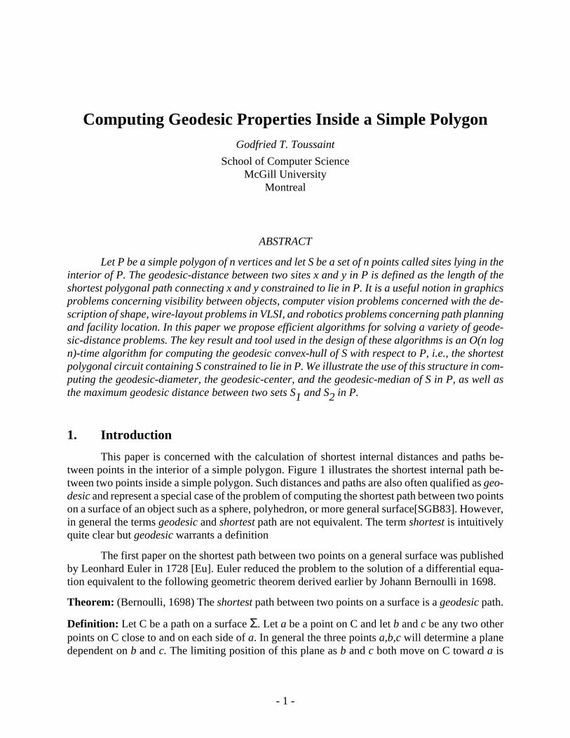
Fig. 1: Illustrating the shortest inter-nal path between two points x and y ina simple polygon P.

- 1 -

Computing Geodesic Properties Inside a Simple PolygonGodfried T. Toussaint

School of Computer ScienceMcGill University

Montreal

ABSTRACT

Let P be a simple polygon of n vertices and let S be a set of n points called sites lying in theinterior of P. The geodesic-distance between two sites x and y in P is defined as the length of theshortest polygonal path connecting x and y constrained to lie in P. It is a useful notion in graphicsproblems concerning visibility between objects, computer vision problems concerned with the de-scription of shape, wire-layout problems in VLSI, and robotics problems concerning path planningand facility location. In this paper we propose efficient algorithms for solving a variety of geode-sic-distance problems. The key result and tool used in the design of these algorithms is an O(n logn)-time algorithm for computing the geodesic convex-hull of S with respect to P, i.e., the shortestpolygonal circuit containing S constrained to lie in P. We illustrate the use of this structure in com-puting the geodesic-diameter, the geodesic-center, and the geodesic-median of S in P, as well asthe maximum geodesic distance between two sets S1 and S2 in P.

1. Introduction

This paper is concerned with the calculation of shortest internal distances and paths be-tween points in the interior of a simple polygon. Figure 1 illustrates the shortest internal path be-tween two points inside a simple polygon. Such distances and paths are also often qualified as geo-desic and represent a special case of the problem of computing the shortest path between two pointson a surface of an object such as a sphere, polyhedron, or more general surface[SGB83]. However,in general the terms geodesic and shortest path are not equivalent. The term shortest is intuitivelyquite clear but geodesic warrants a definition

The first paper on the shortest path between two points on a general surface was publishedby Leonhard Euler in 1728 [Eu]. Euler reduced the problem to the solution of a differential equa-tion equivalent to the following geometric theorem derived earlier by Johann Bernoulli in 1698.

Theorem: (Bernoulli, 1698) The shortest path between two points on a surface is a geodesic path.

Definition: Let C be a path on a surface Σ. Let a be a point on C and let b and c be any two otherpoints on C close to and on each side of a. In general the three points a,b,c will determine a planedependent on b and c. The limiting position of this plane as b and c both move on C toward a is