1

Term Structure of Commodities Futures. Forecasting and Pricing.

Marcos Escobar, Nicolás Hernández, Luis Seco

RiskLab, University of Toronto

Abstract

The development of risk management methodologies for non-gaussian

markets relies often on the assumption that the underlying market factors

have a gaussian distribution. While advances have been made in the

modeling of more general marginal distributions of the risk factors, the

modeling of non-gaussian dependence structures is much less advanced.

For commodities markets that often exhibit sudden changes from

backwardation into contango (such as energy, agricultural products and

metals), correlations or linear transformations of them fail to account for

realistic transformations of forward curve convexity. This paper develops

a model that overcomes this difficulty for scenario generation purposes. It

also provides the “risk neutral” processes needed for derivatives pricing,

answering two leading problems of the financial world (forecasting and

pricing), and presents it in the context of other developments for

commodity futures modeling.

2

I - INTRODUCTION

The development of risk management methodologies for non-gaussian markets relies often on

the assumption that the underlying market factors have a gaussian distribution. While advances

have been made in the development of more flexible families of distributions to model the

marginal behavior of the risk factors, the modeling of non-gaussian dependence structures is

much less advanced. Normal rank correlations (NRC) and Spearman ratios, over the underlyngs

factors or directly over the observed curve, in general yield better results than correlations in

markets with non-gaussian marginals, but are still linear-based measures of dependence. For

commodities markets that often exhibit sudden changes from backwardation into contango (such

as energy, agricultural products and metals), they fail to account for realistic transformations of

future curve convexity. Copulas, which in principle will reconstruct the entire dependence

structure, appear to be too difficult to impractical in specific situations.

This paper develops a model that overcomes this difficulty in certain markets, and

presents it in the context of related developments for commodity futures modeling. The first step

will provide a model to fit commodity markets for the purpose of scenario generation in the

context of risk management exercises; in order to enhance the scope of the proposed model, as a

second step, “non-arbitrage conditions” will be considered with purposes of pricing commodities

derivatives.

Lets first point out the followings practical facts about futures markets in commodities: 1 – A commodity’s future contract is an agreement to exchange a fixed amount of physical asset

for a specific price at maturity T.

3

2 - Futures contract are traded in a day-by-day basis, and there are widely known conventions

about how they should be traded; this is not the case of the forward contract, which is only found

on over the counter markets.

3 – One of the most influent features of the futures markets is that you can only get at time-t the

future prices for a commodity maturing at Ti-t for fixed values of Ti, i.e. Ti are the 20th of every

month in the case of oil.

There are two popular views of commodities prices; both based on the fitting of the

observed term structure for futures prices, namely:

By modeling the vector of futures prices of dimension m (12 in Oil case) that can be obtained at

any time-t from the market, filtering all types of dependencies trough time in the components of

the vector and taking care of the multivariate structure of the residuals by NRC or Spearman

ratios. This is the simplest way, but fail to account for the arbitrage-free conditions.

The theory of storage (TS) of Kaldor (1939), Brennan (1958) and Telser (1958) explains the

difference between contemporaneous spot and the futures prices in terms of interest forgone in

storing a commodity, warehousing costs, and a convenience yield on inventory. This can be also

seemed as a multiplicative model. They obtained processes for the underlyngs under “arbitrage-

free” conditions.

4

In this article we will present an alternative to the previous methods, but first we will basically

review TS and the statistical features of the futures prices vectors.

There is one general way to obtain expression for the futures prices of commodities under

The Theory of Storage:

))}(,(),(),({

,tTTtTtuTtr

tTt eSF −−+= δ,

where:

TtF , denotes the future price, at time t of a contract for delivery at time T.

tS is the spot price of the commodity at time t.

),( Ttr is the interest rate at time t for (T-t) time to maturity, bootstrapped from the zero curve.

),( Ttδ is the convenience yield: the flow of services that accrues to the holder of the physical

commodity, but not to the owner of a contract for future delivery. In others words the benefit

from ownership of the physical commodity that may include the ability to profit from temporary

local storages or the ability to keep a production process running, at time-t for (T-t)-time to

maturity.

),( Ttu is the storage cost at time t for (T-t)-time to maturity. The instantaneous interest rate and instantaneous convenience yield are defined as

T t T tl i m ( , ) , l i m ( , )t tr r t T t Tδ δ

↓ ↓= = respectively.

The term structures of forward interest rate and futures convenience yields are defined as

T s T s( , ) l im ( , , ) , ( , ) l im ( , , )r f t s r t s T f t s t s Tδ δ

↓ ↓= = respectively.

5

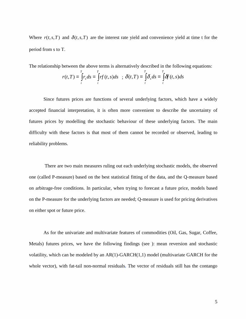
Where ),,( Tstr and ),,( Tstδ are the interest rate yield and convenience yield at time t for the

period from s to T.

The relationship between the above terms is alternatively described in the following equations:

∫∫ ==T

t

T

ts dsstrfdsrTtr ),(),( ; ∫∫ ==

T

t

T

ts dsstfdsTt ),(),( δδδ

Since futures prices are functions of several underlying factors, which have a widely

accepted financial interpretation, it is often more convenient to describe the uncertainty of

futures prices by modelling the stochastic behaviour of these underlying factors. The main

difficulty with these factors is that most of them cannot be recorded or observed, leading to

reliability problems.

There are two main measures ruling out each underlying stochastic models, the observed

one (called P-measure) based on the best statistical fitting of the data, and the Q-measure based

on arbitrage-free conditions. In particular, when trying to forecast a future price, models based

on the P-measure for the underlying factors are needed; Q-measure is used for pricing derivatives

on either spot or future price.

As for the univariate and multivariate features of commodities (Oil, Gas, Sugar, Coffee,

Metals) futures prices, we have the following findings (see ): mean reversion and stochastic

volatility, which can be modeled by an AR(1)-GARCH(1,1) model (multivariate GARCH for the

whole vector), with fat-tail non-normal residuals. The vector of residuals still has the contango

6

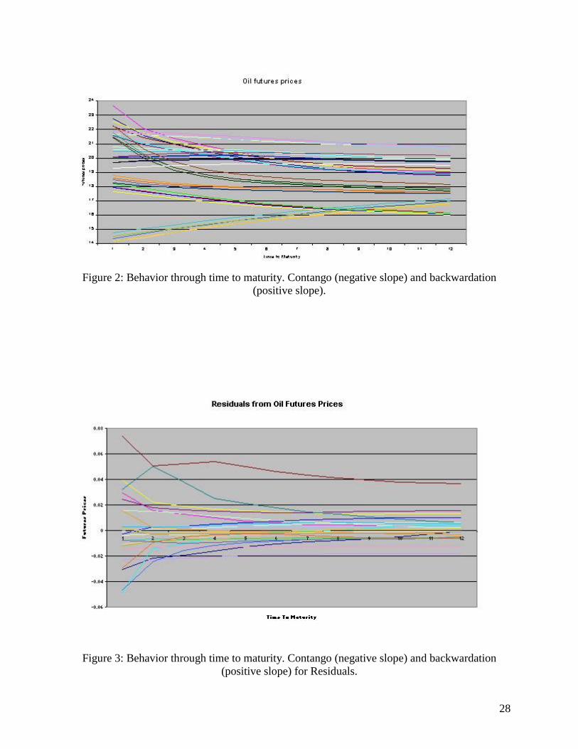
and backwardation feature (increasing or decreasing curve trough time-to-maturity) see figure 3

for Residuals from a Vector Autoregressive.

This paper propose an additive (quadratic fitting) model for the term structure of futures prices

leading to a 3-dim vector of underlyngs. These new factors are studied, showing simple

stochastic behaviour and normal dependency structures under the real measure. They are also

modelled under “arbitrage free” conditions for purposes of pricing derivatives. This model shows

more accurate forecasting than AR-GARCH models, getting a better and more flexible fitting,

for up to 1 year time-to-maturity, of the term structure of futures prices, volatilities and

correlations than TS models.

The paper is organized as follows: The second section is a survey of some of the most important

models (given explicitly the Q-measure for the underlying, the P-measure is basically zero

market price of risk, λ=0,) in the literature, highlighting some of their drawbacks: Schwartz

1997, Miltersen and Schwartz 1998, Thomas Urich 2000 and Schwartz-Smith 2000. Section III

deals with the proposed model and some details about the estimation procedure. The fourth

section is dedicated to the forecasting properties of the model using a test portfolio and measures

of risk implemented in RiskWatch 3.2.6 and HistoRisk 1.6, software developed by Algorithmics

Inc for risk management purposes The fifth section deals with the formalization of the pricing

framework for the proposed model. Section sixth deals with the volatilities and correlations

implied by our model over the future prices term structure, and last section goes to the pricing of

options on futures contracts.

7

II - MODELS

One of the difficulties in the empirical implementation of commodity price models is that

frequently the factors or state variables of these models are not directly observable. For some

commodities the spot price is hard to obtain, and the futures contract closest to maturity is used

as proxy for the spot price. The problems of estimating the instantaneous convenience yield are

even more complex; normally, futures prices with different maturities are used to compute it.

The instantaneous interest rate is also not directly observable. Futures contracts, however, are

widely traded in several exchanges and their prices are more easily observed. This is why a

model based on modelling directly futures prices is more convenient and reliable.

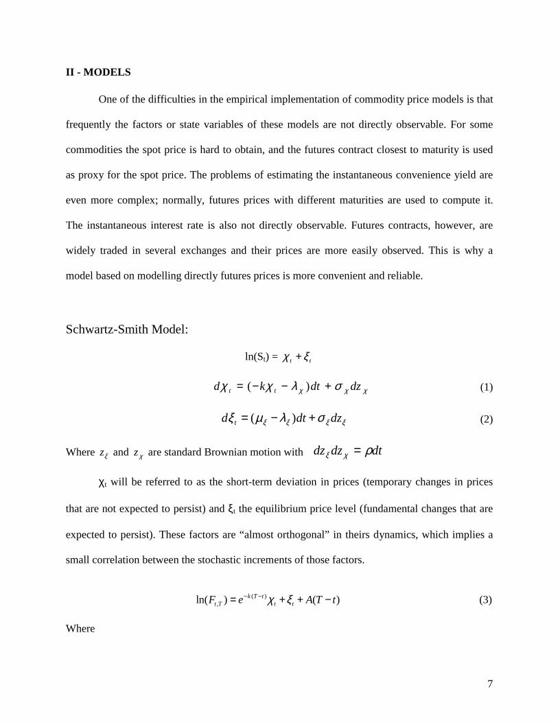
Schwartz-Smith Model:

ln(St) = tt ξχ +

χχχ σλχχ dzdtkd tt +−−= )( (1)

ξξξξ σλµξ dzdtd t +−= )( (2) Where ξz and χz are standard Brownian motion with dtdzdz ρχξ =

χt will be referred to as the short-term deviation in prices (temporary changes in prices

that are not expected to persist) and ξt the equilibrium price level (fundamental changes that are

expected to persist). These factors are “almost orthogonal” in theirs dynamics, which implies a

small correlation between the stochastic increments of those factors.

( )

,ln( ) ( )k T tt T t tF e A T tχ ξ− −= + + − (3)

Where

8

−+−+−+−−−=− −−−−−−

ketT

ke

ketTtTA tTktTktTk ρσσ

σσλ

µ ξχξ

χχξ )1(2)(

2)1(

21)1()()( )(2

2)(2)(*

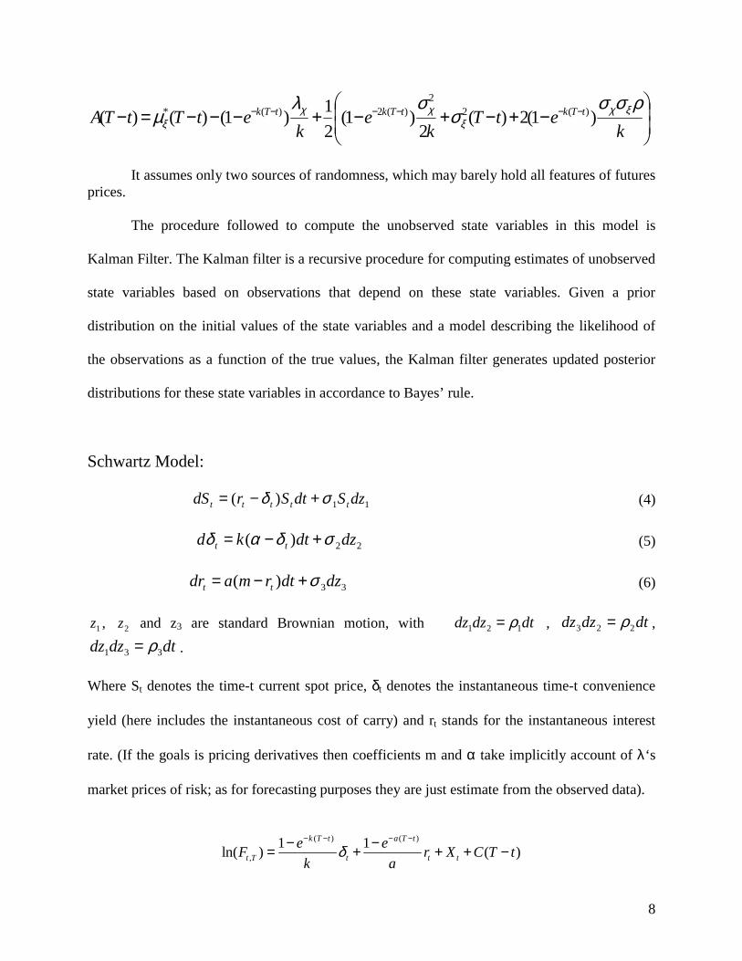
It assumes only two sources of randomness, which may barely hold all features of futures

prices.

The procedure followed to compute the unobserved state variables in this model is

Kalman Filter. The Kalman filter is a recursive procedure for computing estimates of unobserved

state variables based on observations that depend on these state variables. Given a prior

distribution on the initial values of the state variables and a model describing the likelihood of

the observations as a function of the true values, the Kalman filter generates updated posterior

distributions for these state variables in accordance to Bayes’ rule.

Schwartz Model:

11)( dzSdtSrdS ttttt σδ +−= (4)

22)( dzdtkd tt σδαδ +−= (5)

33)( dzdtrmadr tt σ+−= (6)

1z , 2z and z3 are standard Brownian motion, with dtdzdz 121 ρ= , dtdzdz 223 ρ= , dtdzdz 331 ρ= .

Where St denotes the time-t current spot price, δt denotes the instantaneous time-t convenience

yield (here includes the instantaneous cost of carry) and rt stands for the instantaneous interest

rate. (If the goals is pricing derivatives then coefficients m and α take implicitly account of λ‘s

market prices of risk; as for forecasting purposes they are just estimate from the observed data).

( ) ( )

,1 1ln( ) ( )

k T t a T t

t T t t te eF r X C T tk a

δ− − − −− −= + + + −

9

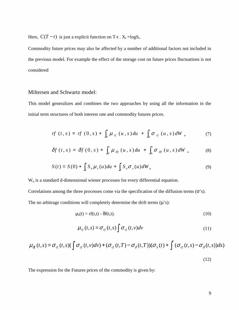
Here, )( tTC − is just a explicit function on T-t . Xt =logSt. Commodity future prices may also be affected by a number of additional factors not included in

the previous model. For example the effect of the storage cost on future prices fluctuations is not

considered

Miltersen and Schwartz model: This model generalizes and combines the two approaches by using all the information in the

initial term structures of both interest rate and commodity futures prices.

∫∫ ++=t

urf

t

rf dWsudususrfstrf00

),(),(),0(),( σµ (7)

∫∫ ++=t

uf

t

f dWsudususfstf00

),(),(),0(),( δδ σµδδ (8)

∫∫ ++=t

usu

t

su dWuSduuSStS00

)()()0()( σµ (9)

Wu is a standard d-dimensional wiener processes for every differential equation. Correlations among the three processes come via the specification of the diffusion terms (σ’s). The no arbitrage conditions will completely determine the drift terms (µ’s):

µs(t) = rf(t,t) - δf(t,t). (10)

∫=s

t rfrfrf dvvtstst ),(),(),( σσµ (11)

))),(),(()())(,(),(()),()(,(),( ∫∫ −+−+=T

t rfSrf

s

t rfrff dsststtTtTtdvvtstst δδδ σσσσσσσµ

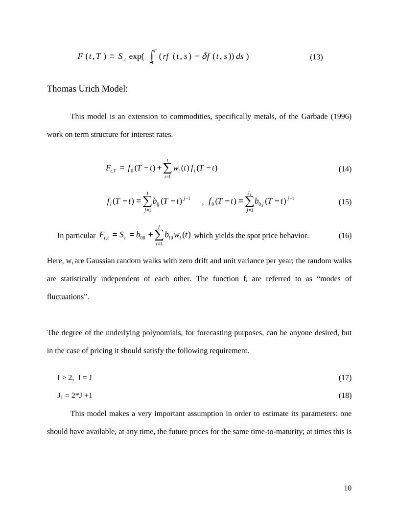
(12) The expression for the Futures prices of the commodity is given by:

10

))),(),((exp(),( ∫ −=T

tt dsstfstrfSTtF δ (13)

Thomas Urich Model:

This model is an extension to commodities, specifically metals, of the Garbade (1996)

work on term structure for interest rates.

)()()(1

0, tTftwtTfFI

iiiTt −+−= ∑

= (14)

∑=

−−=−J

j

jiji tTbtTf

1

1)()( , ∑=

−−=−1

1

100 )()(

J

j

jj tTbtTf (15)

In particular ∑=

+==I

iiittt twbbSF

1000, )( which yields the spot price behavior. (16)

Here, wi are Gaussian random walks with zero drift and unit variance per year; the random walks

are statistically independent of each other. The function fi are referred to as “modes of

fluctuations”.

The degree of the underlying polynomials, for forecasting purposes, can be anyone desired, but

in the case of pricing it should satisfy the following requirement.

I > 2, I = J (17)

J1 = 2*J +1 (18)

This model makes a very important assumption in order to estimate its parameters: one

should have available, at any time, the future prices for the same time-to-maturity; at times this is

11

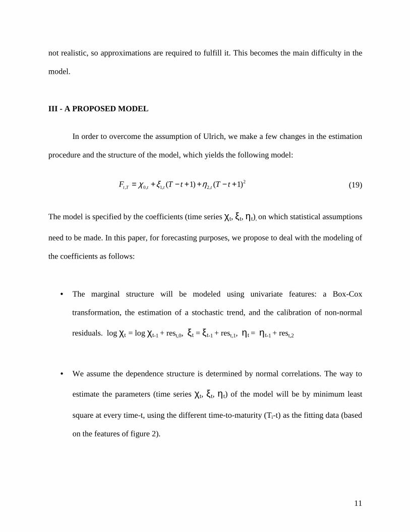
not realistic, so approximations are required to fulfill it. This becomes the main difficulty in the

model.

III - A PROPOSED MODEL

In order to overcome the assumption of Ulrich, we make a few changes in the estimation

procedure and the structure of the model, which yields the following model:

2

, 0, 1, 2,( 1) ( 1)t T t t tF T t T tχ ξ η= + − + + − + (19) The model is specified by the coefficients (time series χt, ξt, ηt), on which statistical assumptions

need to be made. In this paper, for forecasting purposes, we propose to deal with the modeling of

the coefficients as follows:

• The marginal structure will be modeled using univariate features: a Box-Cox

transformation, the estimation of a stochastic trend, and the calibration of non-normal

residuals. log χt = log χt-1 + rest,0, ξt = ξt-1 + rest,1, ηt = ηt-1 + rest,2

• We assume the dependence structure is determined by normal correlations. The way to

estimate the parameters (time series χt, ξt, ηt) of the model will be by minimum least

square at every time-t, using the different time-to-maturity (Ti-t) as the fitting data (based

on the features of figure 2).

12

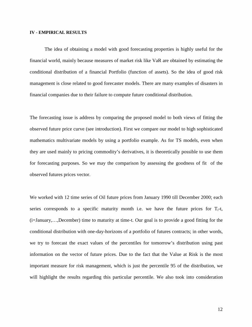
IV - EMPIRICAL RESULTS

The idea of obtaining a model with good forecasting properties is highly useful for the

financial world, mainly because measures of market risk like VaR are obtained by estimating the

conditional distribution of a financial Portfolio (function of assets). So the idea of good risk

management is close related to good forecaster models. There are many examples of disasters in

financial companies due to their failure to compute future conditional distribution.

The forecasting issue is address by comparing the proposed model to both views of fitting the

observed future price curve (see introduction). First we compare our model to high sophisticated

mathematics multivariate models by using a portfolio example. As for TS models, even when

they are used mainly to pricing commodity’s derivatives, it is theoretically possible to use them

for forecasting purposes. So we may the comparison by assessing the goodness of fit of the

observed futures prices vector.

We worked with 12 time series of Oil future prices from January 1990 till December 2000; each

series corresponds to a specific maturity month i.e. we have the future prices for Ti-t,

(i=January,…,December) time to maturity at time-t. Our goal is to provide a good fitting for the

conditional distribution with one-day-horizons of a portfolio of futures contracts; in other words,

we try to forecast the exact values of the percentiles for tomorrow’s distribution using past

information on the vector of future prices. Due to the fact that the Value at Risk is the most

important measure for risk management, which is just the percentile 95 of the distribution, we

will highlight the results regarding this particular percentile. We also took into consideration

13

other percentiles than the 95: if a portfolio depends on futures prices in a non-linear way (i.e.

options on futures), then small percentiles may have an influence in the portfolio Var.

Lets introduce the following notation:

Distα (Pt / t-1): Percentile α of the conditional distribution of the Portfolio P for time t, given

information available at time t-1.

Pt - Observed value for Portfolio P at day t.

The following test is equivalent to the one explained in Diebold, which is based on the iid U(0,1)

properties of the probability integral transform series ( , 1)tt P tz Dist P t= − .

The number of time that the real value of the Portfolio (Pt) is bigger than Distα (Pt / t-1) for a

given percentiles α (i.e. 95%) out of 250 replicas should be close to 250(1-α)/100, (12.5). So, by

the creation of the following Bernoulli random variable, we will be able to assess how well is

every percentile recovered (test of goodness-of-forecasting) .

Biα = 1 if Pi > Distα (Pi / i-1)

0 otherwise. Let create the following graph representation, percentiles from 0.01 to 0.99 are allocated in the

X-axis, numbers Yiα = (∑=

250

1iiB α )/ (250*α) are allocated in the Y-axis.

So pairs (α,∑=

250

1iiB α ) or (α,Yiα ) show the behaviour of the whole conditional distribution for the

Portfolio. We will use (α,Yiα ) in table I as a comparative tools. The closer to one the values of

Yiα , the better the model in its forecasting abilities. As has been suggested by Diebold (1998),

14

the previous visual assessment is more revealing, constructive and attractive than more

sophisticated procedures such as kernel density estimates.

A portfolio was created using RiskWatch software, three instruments were created, a

commodity forward starting at 23-08-1998 and maturing at 90 days, the second one starting at

the same moment and maturing at 120 days and the last one with the same start date and maturity

250 (business) days.

Fourth sets of scenarios were created following different models. Two of them come

from considering the residuals rest to be normal/non-normal or dependent/independent in our

model. Also we created two set of scenarios based on different assumptions for the vector of

futures prices.

1. Empirical Distribution of the residuals (rest) in proposed model, taking into account last

250 values. (EP250)

2. Normal Distribution of the residuals (rest) in proposed model, taking into account last

250 values. (ND250)

3. Mean reversion and Garch in every univariate future prices series, multivariate normal

for the residuals (using principal components) from the AR(1)-Garch(1,1), 250 previous

values considered. (MRGN)

4. Mean reversion and Garch in every univariate future prices series, Empirical distribution

for the multivariate residuals from the AR(1)-Garch(1,1), 250 previous values

considered. (MRGEP)

15

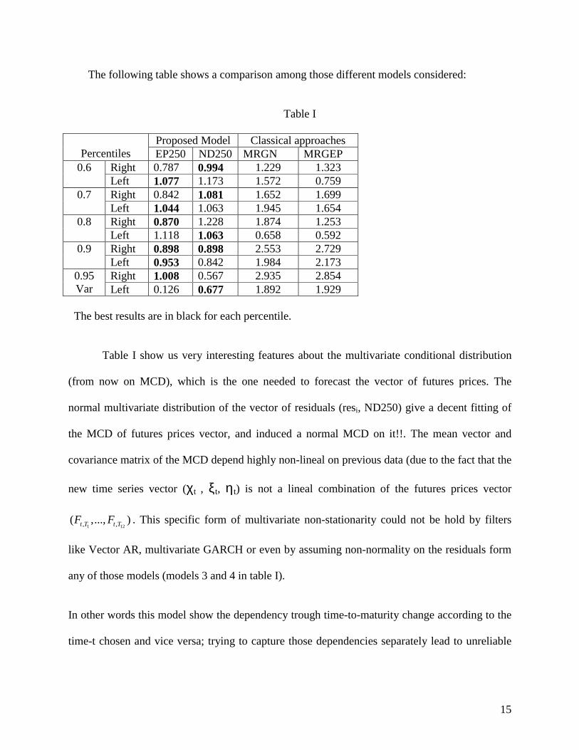
The following table shows a comparison among those different models considered:

Table I

Proposed Model Classical approaches Percentiles EP250 ND250 MRGN MRGEP

Right 0.787 0.994 1.229 1.323 0.6 Left 1.077 1.173 1.572 0.759 Right 0.842 1.081 1.652 1.699 0.7 Left 1.044 1.063 1.945 1.654 Right 0.870 1.228 1.874 1.253 0.8 Left 1.118 1.063 0.658 0.592 Right 0.898 0.898 2.553 2.729 0.9 Left 0.953 0.842 1.984 2.173 Right 1.008 0.567 2.935 2.854 0.95

Var Left 0.126 0.677 1.892 1.929 The best results are in black for each percentile. Table I show us very interesting features about the multivariate conditional distribution

(from now on MCD), which is the one needed to forecast the vector of futures prices. The

normal multivariate distribution of the vector of residuals (resi, ND250) give a decent fitting of

the MCD of futures prices vector, and induced a normal MCD on it!!. The mean vector and

covariance matrix of the MCD depend highly non-lineal on previous data (due to the fact that the

new time series vector (χt , ξt, ηt) is not a lineal combination of the futures prices vector

1 12, ,( ,..., )t T t TF F . This specific form of multivariate non-stationarity could not be hold by filters

like Vector AR, multivariate GARCH or even by assuming non-normality on the residuals form

any of those models (models 3 and 4 in table I).

In other words this model show the dependency trough time-to-maturity change according to the

time-t chosen and vice versa; trying to capture those dependencies separately lead to unreliable

16

results, leading us to think that the behavior in t and T-t should be faced simultaneously using the

contango and backwardation features of the futures price vector.

Regarding TS models, the standard deviation of the error (obtained from the regressions) is

smaller for the quadratic polynomial (additive model) than for the Schwarz model (multiplicative

model). The goodness of fit from exponential function is worse that the fitting using quadratic

polynomials in the time-to-maturity considered (1 year) .

V - COMMODITY DERIVATIVE PRICING Lets mention a couple of examples that address the importance of taking care of the contango-

backwardation feature in the pricing of derivatives.

Metalgesellschaft: 1993 It decided to market long dated futures contracts to US clients (up to 30

years), when the market only had futures up to 18 months. Their strategy relied on rolling over

the contracts at expiration. A change in the convexity of the futures curve gave rise to margin

payments that they could not meet. They lost over $1B.

Orange County and Bob Citron: In December 1994, Orange County stunned the markets by

announcing that its investment pool had suffered a loss of $1.6 billion, the largest loss ever

recorded by a local government investment pool, and led to the bankruptcy of the county. This

loss was the result of unsupervised investment activity of Bob Citron, the County Treasurer, who

was entrusted with an $7.5 billion portfolio belonging to county schools, cities, special districts

17

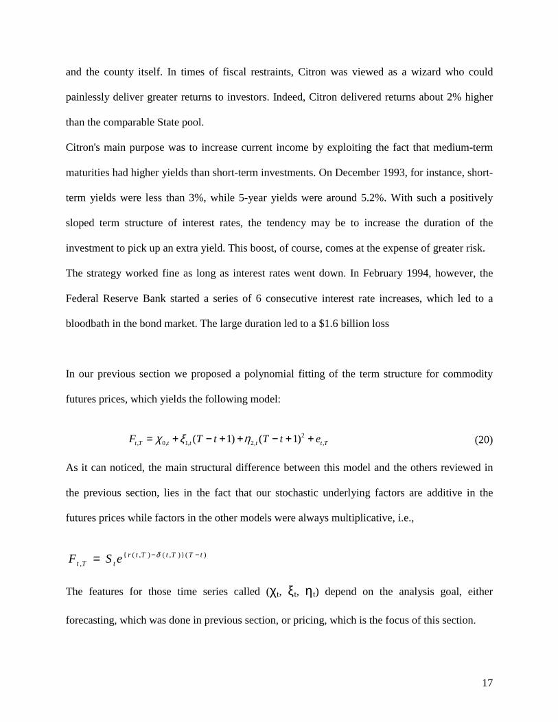
and the county itself. In times of fiscal restraints, Citron was viewed as a wizard who could

painlessly deliver greater returns to investors. Indeed, Citron delivered returns about 2% higher

than the comparable State pool.

Citron's main purpose was to increase current income by exploiting the fact that medium-term

maturities had higher yields than short-term investments. On December 1993, for instance, short-

term yields were less than 3%, while 5-year yields were around 5.2%. With such a positively

sloped term structure of interest rates, the tendency may be to increase the duration of the

investment to pick up an extra yield. This boost, of course, comes at the expense of greater risk.

The strategy worked fine as long as interest rates went down. In February 1994, however, the

Federal Reserve Bank started a series of 6 consecutive interest rate increases, which led to a

bloodbath in the bond market. The large duration led to a $1.6 billion loss

In our previous section we proposed a polynomial fitting of the term structure for commodity

futures prices, which yields the following model:

2

, 0, 1, 2, ,( 1) ( 1)t T t t t t TF T t T t eχ ξ η= + − + + − + + (20) As it can noticed, the main structural difference between this model and the others reviewed in

the previous section, lies in the fact that our stochastic underlying factors are additive in the

futures prices while factors in the other models were always multiplicative, i.e.,

{ ( , ) ( , )}( )

,r t T t T T t

t T tF S e δ− −= The features for those time series called (χt, ξt, ηt) depend on the analysis goal, either

forecasting, which was done in previous section, or pricing, which is the focus of this section.

18

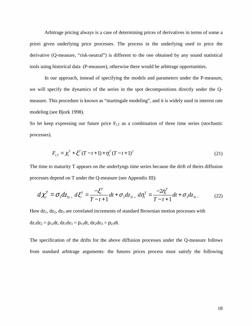
Arbitrage pricing always is a case of determining prices of derivatives in terms of some a

priori given underlying price processes. The process in the underlying used to price the

derivative (Q-measure, “risk-neutral”) is different to the one obtained by any sound statistical

tools using historical data (P-measure), otherwise there would be arbitrage opportunities.

In our approach, instead of specifying the models and parameters under the P-measure,

we will specify the dynamics of the series in the spot decompositions directly under the Q-

measure. This procedure is known as “martingale modeling”, and it is widely used in interest rate

modeling (see Bjork 1998).

So let keep expressing our future price Ft,T as a combination of three time series (stochastic

processes).

2

, ( 1) ( 1)T T Tt T t t tF T t T tχ ξ η= + − + + − + (21)

The time to maturity T appears on the underlyngs time series because the drift of theirs diffusion

processes depend on T under the Q-measure (see Appendix III):

1 1Tt td dzχ σ= , 2 21

TT tt td dt dz

T tξξ σ−= +

− + , 3 32

1

TT tt td dt dz

T tηη σ−= +

− + . (22)

Here dz1, dz2, dz3 are correlated increments of standard Brownian motion processes with

dz1dz2 = ρ12dt, dz1dz3 = ρ13dt, dz2dz3 = ρ23dt.

The specification of the drifts for the above diffusion processes under the Q-measure follows

from standard arbitrage arguments: the futures prices process must satisfy the following

19

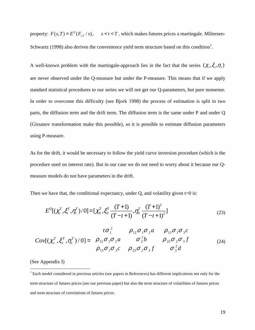
property: ,( , ) ( / ) ,Qt TF s T E F s s t T= < < , which makes futures prices a martingale. Miltersen-

Schwartz (1998) also derives the convenience yield term structure based on this condition1.

A well-known problem with the martingale-approach lies in the fact that the series ),,( ttt ηξχ

are never observed under the Q-measure but under the P-measure. This means that if we apply

standard statistical procedures to our series we will not get our Q-parameters, but pure nonsense.

In order to overcome this difficulty (see Bjork 1998) the process of estimation is split in two

parts, the diffusion term and the drift term. The diffusion term is the same under P and under Q

(Girsanov transformation make this possible), so it is possible to estimate diffusion parameters

using P-measure.

As for the drift, it would be necessary to follow the yield curve inversion procedure (which is the

procedure used on interest rate). But in our case we do not need to worry about it because our Q-

measure models do not have parameters in the drift.

Then we have that, the conditional expectancy, under Q, and volatility given t=0 is:

2

0 0 0 2

( 1) ( 1)[( , , ) /0] [ , , ]( 1) ( 1)

Q T T T T T Tt t t

T TET t T t

χ ξ η χ ξ η+ +=− + − + (23)

[( , , ) / 0]T T Tt t tCov χ ξ η =

dfcfbacat

2332233113

3223222112

311321122

1

σσσρσσρσσρσσσρσσρσσρσ

(24)

(See Appendix I) 1 Each model considered in previous articles (see papers in References) has different implications not only for the

term structure of futures prices (see our previous paper) but also the term structure of volatilities of futures prices

and term structure of correlations of futures prices.

20

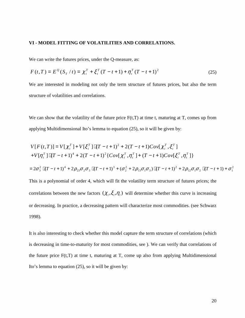
VI - MODEL FITTING OF VOLATILITIES AND CORRELATIONS. We can write the futures prices, under the Q-measure, as:

2( , ) ( / ) ( 1) ( 1)Q T T TT t t tF t T E S t T t T tχ ξ η= = + − + + − + (25)

We are interested in modeling not only the term structure of futures prices, but also the term

structure of volatilities and correlations.

We can show that the volatility of the future price F(t,T) at time t, maturing at T, comes up from

applying Multidimensional Ito’s lemma to equation (25), so it will be given by:

2

4 2

[ ( , )] [ ] [ ] ( 1) 2( 1) [ , ]

[ ] ( 1) 2( 1) { [ , ] ( 1) [ , ]}

T T T Tt t t t

T T T T Tt t t t t

V F t T V V T t T t CovV T t T t Cov T t Cov

χ ξ χ ξη χ η ξ η

= + ⋅ − + + − +

+ ⋅ − + + − + + − +

212112

23113

22

33223

423 )1(2)1()2()1(2)1(2 σσσρσσρσσσρσ ++−⋅++−⋅+++−⋅++−⋅= tTtTtTtT

This is a polynomial of order 4, which will fit the volatility term structure of futures prices; the

correlations between the new factors ),,( ttt ηξχ will determine whether this curve is increasing

or decreasing. In practice, a decreasing pattern will characterize most commodities. (see Schwarz

1998).

It is also interesting to check whether this model capture the term structure of correlations (which

is decreasing in time-to-maturity for most commodities, see ). We can verify that correlations of

the future price F(t,T) at time t, maturing at T, come up also from applying Multidimensional

Ito’s lemma to equation (25), so it will be given by:

21

2/1)]},([)],([{)],(),,([)],(),,([

StFVTtFVStFTtFCovStFTtFCorr

⋅= , where the covariance is given by:

23

223223

2222

311322

211221

)1()1(

])1)(1()1)(1[()1)(1(

])1()1[()22()],(),,([

σσσρσ

σσρσσρσ

+−+−+

+−+−++−+−++−+−+

+−++−++−++=

tStTtTtStStTtStT

tTtStSTStFTtFCov

This is a quotient of polynomial on two variables of order 4, which will fit the correlations term

structure of the futures prices; the correlation on the unobserved series will determine whether

this structure is increasing or decreasing.

For example, lets consider a lineal model (only ),( tt ξχ , no quadratic term). We will get the

following polynomial of order two for the volatility of futures:

212112

222 )1(2)1( σσσρσ ++−⋅++−⋅ tTtT , Which means decreasing volatility in the interval

)]1(,[)1(21

212

122

1 −−−−∞∈+−σσ

ρρσσ

tT , and increasing in the interval

]),1([)1(21

212

122

1 +∞−+−∈+−σσ

ρρσσ

tT , in case of negative correlation.

We will also get the following polynomial of order two for the correlations of futures:

2/1212112

222

212112

222

222112

21

]})1(2)1([])1(2)1({[)1)(1()22(

σσσρσσσσρσσσσρσ

++−⋅++−⋅⋅++−⋅++−⋅+−+−++−++

tStStTtTtStTtST

The correlation for ),( tt ξχ , using real futures prices from 1996 till 1999, was –0.89, which

implies decreasing volatilities and also decreasing correlations from 0 year till 1 year time-to-

maturity.

VII - VALUING OPTIONS ON FUTURES CONTRACTS

22

A future contract, started at 0, is define as the following contingent claim (also called a T-claim

due to the dependency only on Time-T): ST-F(0,T). A European option on a spot is a T-claim

defined as Max{ST-K, 0}; a European option with exercise date T on a future contract (maturing

at T1) is a T-claim defined as Max{F(T,T1)-K, 0}. K is always the accorded price.

From the formula for current futures prices:

2( , ) ( / ) ( 1) ( 1)Q T T TT t t tF t T E S t T t T tχ ξ η= = + − + + − + . Given current state variables at

0, because they are jointly normally distributed at t, we get:

2

0 0 0 2

( 1) ( 1)( , ) [ ( , ) / 0]( 1) ( 1)

Q T Tt T E F t TT t T t

µ χ ξ η+ += = + ⋅ + ⋅− + − +

(27)

2 2

4 2

( , ) [ ( , )] [ ] [ ] ( 1) 2( 1) [ , ]

[ ] ( 1) 2( 1) [ ( 1) , ]

T T T Tt t t t

T T T Tt t t t

t T V F t T V V T t T t Cov

V T t T t Cov T t

σ χ ξ χ ξη χ ξ η

= = + ⋅ − + + − +

+ ⋅ − + + − + + − + (28)

The variance and covariance given time 0 are the results shown in matrix (24).

The value of a European option on a futures contract maturing at time T, with strike price K, and

time t until the option expires is (under constant interest rate):

[max( ( , ) ,0)]rt Qe E F t T K− − . (29)

Closed form expression for the price of a European option on a future contract. Assume that F(t,T) ~ N(µ(t,T), σ2(t,T)) , this implies that µσ +⋅ F ~ N(0,1). Lets call the

density function of a N(0,1) as ϕ. Then the expected part, under the equivalent measure, of an

option value at moment 0 is:

23

))0(1()),((2

),(2

)(

)()]0,[max(

2)0(

02

22

zNKTteTtdzeKz

dzzKzz

z

z

−⋅−+⋅=−+⋅=

⋅⋅−+⋅

−∞ −

∞

∞−

∫

∫

µπ

σπµσ

ϕµσ

(30)

Where, σ

µ−= KZ0 and ∫ ∞−=

xdzzxN )()( ϕ .

VIII - CONCLUSIONS

1. The most influent characteristic in a Portfolio of Oil forwards (futures) is the multivariate

dependency structure; this leaded us to focus in the search for a model holding this

feature.

2. The models proposed in the literature do not focus on both goals forecasting and pricing,

besides they have, as mains problems:

-Inaccuracy in the input data (i.e. errors on the estimated spot prices, instantaneous

convenience yields).

-Unrealistic assumptions (i.e. futures prices for the same time-to-maturity at every

time-t).

-Do not take into considerations the storage cost as a stochastic process and even do

not allow new sources of randomness to show up (TS).

3. The proposed model work straight with the spot prices (not the log of spot prices)

implying addition model instead of multiplicative model for the futures prices. It is the

first model that provides an additive explanation for the term structure of futures prices of

Commodities.

24

4. Due to being additive, our model can be used for times to maturity up to 1 year, which

actually is the sample used in the estimation procedure. It gives no support for asymptotic

(on time) conclusions.

5. This model only requires estimation of six parameters, being more parsimonious than

other TS model, which requires more free parameters.

6. It provides “arbitrage-free” underlying models for pricing purposes by mixing results

from Schwartz 2000 and Interest rate martingale modeling approach.

��� A multivariate normal distribution in few factors (the ones underlyngs our model) is able

to explain the whole vector of futures prices; these factors are not obtained by principal

components because it is not the correlation what should be conserved.

8. As for univariate forward (spot) Oil time series, we realized the following:

- If the goal is to get a good short-term forecasting then it is better to work with the

returns (log of differencing). There is not significant presence of lineal correlation

(ARMA) on the returns, but there is high correlation in the return square (GARCH(1,1)),

with non-normal residuals.

- As for the medium and long-term forecasting, there is a marked reversion to the mean,

and high correlation in the residuals square (GARCH(1,1)).

- It was not observed deterministic or stochastic seasonality in any case.

9. We may use this model to price derivatives of several underlyngs (commodities like

sugar, oil, etc), looking at the correlations among the constant, linear and quadratic

series.

25

IX – Bibliography. Bjork, T. 1998 Arbitrage theory in continuous time.

Breeden, D.T., 1980, “Consumption risks in futures markets,” Journal of Finance, 35(2): 503–

520, May.

Brennan, M.J., 1958, “The supply of storage,” American Economic Review, 48: 50–72, March.

Brennan, M. J., 1991, “The price of conve-nience and the evaluation of commodity contingent

claims.,” D. Lund, B. Oksendal, (eds.) Stochastic Models and Option Values: Applications to

Resources, Environment, and Investment Problems. New York, NY: North-Holland.

Campbell, Lo and Mackinlay. 1997 “The econometric of financial markets”.

Cootner, P.H., 1960, “Returns to speculators: Telser versus Keynes,” The Journal of Political

Economy, 68: 396–404.

Cortazar, G. and E. Schwartz, 1994, “The valuation of commodity-contingent claims,” The

Journal of Derivatives, 1(4): 27–39.

Diebold, F.X., T.A., Gunther and A.S. Tay, 1998, “Evaluating density forecasts: With

applications to financial risk management,” International Economic Review, 39: 863–883.

Diebold, F.X., J.Y. Hanh and A.S. Tay, 1999, “Multivariate density forecast evalua-

tion and calibration in financial risk management: High-frequency returns on foreign

exchange,” Review of Economics and Statistics, 81: 661–673.

Garbade, K., 1996, Fixed Income Analysis, Cambridge, MA: MIT Press.

26

Gibson, R. and E. S. Schwartz, 1990, “Stochastic convenience yield and the pricing of oil

contingent claims,” Journal of Finance, 45(3): 959–976.

Hazuka, T.B., 1984, “Futures markets: Consumption betas and backwardation in commodity

markets, Journal of Finance, 39(3): 647–655, July.

Hong, H., 2001, “Stochastic convenience yield, optimal hedging and the term structure of open

interest and futures prices,” Working Paper.

Hull, John C., 2000, Options, Futures and Other Derivatives. New Jersey: Prentice Hall.

Kaldor, N.,1939, “Speculation and economic stability,” Review of Economic Studies, 9: 1– 27,

October.

Ross, S.A., 1995, “Hedging long-run commitments: Exercises in incomplete market pricing,”

Preliminary draft.

Schwartz, E. S., 1997, “The stochastic behavior of commodity prices: Implications for valuation

and hedging,” Journal of Finance, 52(3): 923–973.

Schwartz, S., 1998, “Valuing long-term commodity assets,” Financial Management, 27(1): 57–

66.

Schwartz, S. and K. Miltersen, 1998, “Pricing of options on commodity futures with stochastic

term structures of convenience yield and interest rate,” Journal of Financial and Quantitative

Analysis, 33(3): 33–59.

Schwartz, S. and J. Smith, 2000, “Short-term variations and long-term dynamics in commodity

prices, Management Science,46(7): 893–911.

Telser, L.G., 1958, “Futures trading and the storage of cotton and wheat,” Journal of Political

Economy, 66: 233–255.

27

Urich, T., 2000, “Modes of fluctuation in metal futures prices,” The Journal of Futures Markets

20(3): 219–241.

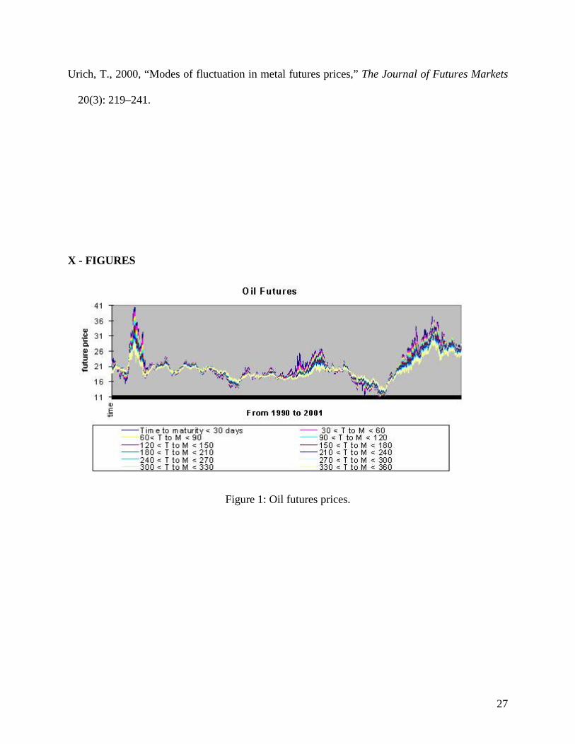
X - FIGURES

Figure 1: Oil futures prices.

28

Figure 2: Behavior through time to maturity. Contango (negative slope) and backwardation

(positive slope).

Figure 3: Behavior through time to maturity. Contango (negative slope) and backwardation

(positive slope) for Residuals.

29

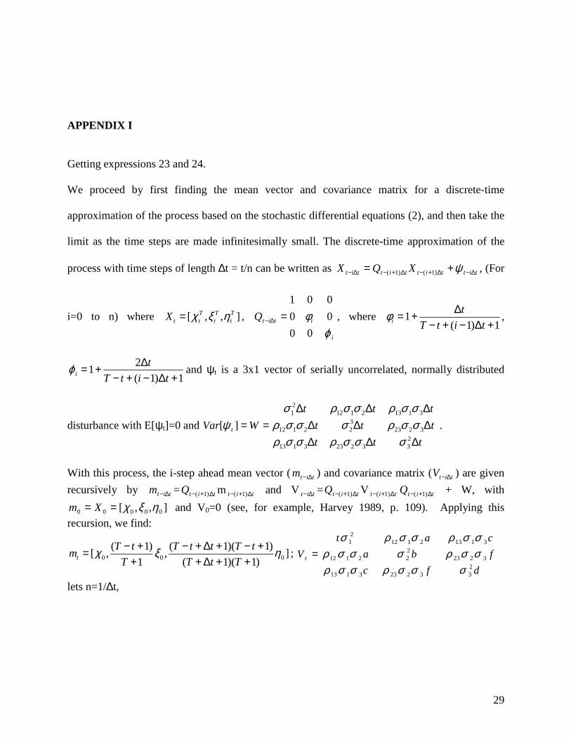
APPENDIX I Getting expressions 23 and 24. We proceed by first finding the mean vector and covariance matrix for a discrete-time

approximation of the process based on the stochastic differential equations (2), and then take the

limit as the time steps are made infinitesimally small. The discrete-time approximation of the

process with time steps of length ∆t = t/n can be written as tittittittit XQX ∆−∆+−∆+−∆− += ψ)1()1( , (For

i=0 to n) where [ , , ]T T Tt t t tX χ ξ η= ,

i

ititQϕ

φ00

00001

=∆− , where 1( 1) 1i

tT t i t

φ ∆= +− + − ∆ +

,

21( 1) 1i

tT t i t

ϕ ∆= +− + − ∆ +

and ψt is a 3x1 vector of serially uncorrelated, normally distributed

disturbance with E[ψt]=0 and ttt

tttttt

WVar t

∆∆∆∆∆∆∆∆∆

==2332233113

3223322112

3113211221

][σσσρσσρ

σσρσσσρσσρσσρσ

ψ .

With this process, the i-step ahead mean vector ( titm ∆− ) and covariance matrix ( titV ∆− ) are given recursively by titm ∆− = titQ ∆+− )1( m tit ∆+− )1( and V tit ∆− = titQ ∆+− )1( V tit ∆+− )1( titQ ∆+− )1( + W, with

],,[ 00000 ηξχ== Xm and V0=0 (see, for example, Harvey 1989, p. 109). Applying this recursion, we find:

0 0 0( 1) ( 1)( 1)[ , , ]

1 ( 1)( 1)tT t T t t T tm

T T t Tχ ξ η− + − + ∆ + − +=

+ + ∆ + +;

dfcfbacat

V t2332233113

3223222112

3113211221

σσσρσσρσσρσσσρσσρσσρσ

=

lets n=1/∆t,

30

1

0 0

{ (1 )}( 1) (1 )

in

i j

t tan j n t n T

−

= =

= +− − + +∑ ∏ ,

12

0 0

{ (1 ) }( 1) (1 )

in

i j

t tbn j n t n T

−

= =

= +− − + +∑ ∏ ,

1

0 0

2{ (1 )}( 1) (1 )

in

i j

t tcn j n t n T

−

= =

= +− − + +∑ ∏ ,

12

0 0

2{ (1 ) }( 1) (1 )

in

i j

t tdn j n t n T

−

= =

= +− − + +∑ ∏ ,

1

0 0

2{ (1 )(1 )}( 1) (1 ) ( 1) (1 )

in

i j

t t tfn j n t n T j n t n T

−

= =

= + +− − + + − − + +∑ ∏

Working with those expressions we found that:

1

0

( 1)( )( 1)

n

i

t it n T tan t n T t

−

=

+ − +=− + − +∑ ,

12

0

( 1){ }( 1)

n

i

t it n T tbn t n T t

−

=

+ − +=− + − +∑ ,

1

0

( 1) ( 1) ( 1)( )( 1) ( 1)

n

i

t it n T t i t n T tcn t n T t n T t

−

=

+ − + − + − +=− + − + − +∑ ,

21

0

( 1) ( 1) ( 1){ }( 1) ( 1)

n

i

t it n T t i t n T tdn t n T t n T t

−

=

+ − + − + − +=− + − + − +∑ ,

12

0

( 1) ( 1) ( 1){[ ] }( 1) ( 1)

n

i

t it n T t i t n T tfn t n T t n T t

−

=

+ − + − + − +=− + − + − +∑

It can be shown that the limit as n goes infinite is:

2

21

ttT ta

T t

− +=

− +;

32

2

( 1)3

( 1)

t t T tb t

T t

+ − += +

− +; c b= ;

3 32

4

2 ( 1)5 3

( 1)

t t T td t

T t

+ − += +

− +;

3 3 22

3

( 1) ( 1)4 3 3

( 1)

t t tT t T tf t

T t

+ − + + − += +

− +.

As can be seen all variables (a,b,c,d,f) depend on t and T. APPENDIX III The following approach is inspired by the work shown on Miltersen-Schwartz (1998). We will

find the stochastic processes for the underlyngs that make the process for F(t,T) a martingale

(zero drift, ,( , ) ( / ) ,Qt TF s T E F s s t T= < < ):

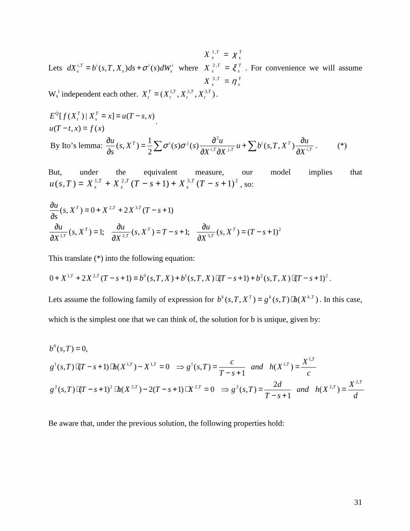
31

Lets , ( , , ) ( )i T i i is s sdX b s T X ds s dWσ= + where

1,

2 ,

3 ,

T Ts s

T Ts s

T Ts s

XXX

χξη

=

=

=

. For convenience we will assume

Wsi independent each other. 1, 2, 3,( , , )T T T T

t t t tX X X X= .

[ ( ) | ] ( , )( , ) ( )

Q T Tt sE f X X x u T s x

u T t x f x= = −

− =.

By Ito’s lemma: 2

, , ,

1( , ) ( ) ( ) ( , , )2

T i j i Ti T j T i T

u u us X s s u b s T Xs X X X

σ σ∂ ∂ ∂= +∂ ∂ ∂ ∂∑ ∑ . (*)

But, under the equivalent measure, our model implies that

1, 2 , 3, 2( , ) ( 1) ( 1)T T Ts s su s T X X T s X T s= + − + + − + , so:

2, 3,

21, 2, 3,

( , ) 0 2 ( 1)

( , ) 1; ( , ) 1; ( , ) ( 1)

T T T

T T TT T T

u s X X X T ssu u us X s X T s s X T s

X X X

∂ = + + − +∂∂ ∂ ∂= = − + = − +

∂ ∂ ∂

This translate (*) into the following equation:

1, 2, 0 1 2 20 2 ( 1) ( , , ) ( , , ) ( 1) ( , , ) ( 1)T TX X T s b s T X b s T X T s b s T X T s+ + − + = + ⋅ − + + ⋅ − + . Lets assume the following family of expression for ,( , , ) ( , ) ( )k T k k Tb s T X g s T h X= ⋅ . In this case,

which is the simplest one that we can think of, the solution for b is unique, given by:

0

1,1 1, 1, 1 1,

2,2 2 2, 2, 2 2,

( , ) 0,

( , ) ( 1) ( ) 0 ( , ) ( )1

2( , ) ( 1) ( ) 2( 1) 0 ( , ) ( )1

TT T T

TT T T

b s Tc Xg s T T s h X X g s T and h X

T s cd Xg s T T s h X T s X g s T and h X

T s d

=

⋅ − + ⋅ − = ⇒ = =− +

⋅ − + ⋅ − − + ⋅ = ⇒ = =− +

Be aware that, under the previous solution, the following properties hold:

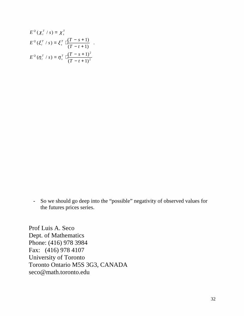
32

2

2

( / )( 1)( / )( 1)( 1)( / )( 1)

Q T Tt s

Q T Tt s

Q T Tt s

E sT sE sT tT sE sT t

χ χ

ξ ξ

η η

=− += ⋅− +− += ⋅− +

.

- So we should go deep into the “possible” negativity of observed values for the futures prices series.

Prof Luis A. Seco Dept. of Mathematics Phone: (416) 978 3984 Fax: (416) 978 4107 University of Toronto Toronto Ontario M5S 3G3, CANADA seco@math.toronto.edu

33

Ph.D Marcos Escobar-Anel Dept. of Mathematics Phone: (416) 946 5808 University of Toronto Toronto Ontario M5S 3G3, CANADA marcos@math.toronto.edu