THE ECONOMICS OF WORLD WAR I: A COMPARATIVEQUANTITATIVE ANALYSIS

Stephen BroadberryDepartment of Economics, University of Warwick, Coventry CV4 7AL, United

KingdomS.N.Broadberry@warwick.ac.uk

and

Mark HarrisonDepartment of Economics, University of Warwick, Coventry CV4 7AL, United

Kingdom, and Hoover Institution on War, Revolution, and Peace, Stanford Universitymark.harrison@warwick.ac.uk

2 August 2005

File: WWItoronto2

Abstract: We draw on the experience of the major combatant countries in World WarI to analyse the role of economic factors in determining the outcome of the war andthe effects of the war on subsequent economic performance. We demonstrate that thedegree of mobilisation for war can be explained largely by differences in the level ofdevelopment of each country, leaving little room for other factors that featureprominently in narrative accounts, such as national differences in war preparations,war leadership, military organisation and morale. We analyse the effects of the war onsubsequent economic performance in terms of the scale of destruction of physical andhuman capital. Although the growth rate between 1918 and 1929 was highest in theeconomies which experienced the worst destruction, over the period 1913-1929 as awhole, per capita income growth in Europe was reduced. Thus there was somerebound, but not enough to undo the negative effects of the capital destruction and thedamage to the international institutional framework caused by the war.

I. INTRODUCTION

There has been little quantitative economic analysis of World War I, and even less

that uses a systematic comparative framework. Although some quantitative work was

conducted at the end of the war under the auspices of the Carnegie Endowment for

International Peace, most of this was organised around individual economies, with

only the study by Bogart (1920) taking a systematic comparative approach.

Subsequent comparative work was either narrowly focused on specific themes such as

public finance (Fisk, 1924; Mendershausen, 1941) or has tended to be rather less

systematically quantitative or economic (Hardach, 1977; Chickering and Förster,

2000). To some extent, previous generations of scholars could point to data problems

as an excuse for not adopting a comparative quantitative approach to the economics of

World War I; the increasing availability of historical national accounts for the major

combatant countries, however, makes this argument no longer sustainable.

In this paper, we draw on the experience of the major combatant countries to

examine the economics of World War I. There was a circle of causation linking total

war and economics, which we decompose into its two halves.

First, we examine the role of economic factors in determining the outcome of the

war. As with our analysis of World War II (Harrison, 1998), we argue that the size of

national resources mattered greatly, but that size was not everything: the quality of the

economy, or its level of development, was also important. The resources of rich

countries were more available for mobilization than the resources of poor countries. If

poor countries tended to get four when they added two and two, rich countries usually

got more. We demonstrate that the degree of mobilisation for war can be explained

largely by differences in the level of development of each country; in other words, the

level of development acted as a multiplier of size. This also leaves little room for

other factors that feature prominently in most narrative accounts, such as national

differences in war preparations, war leadership, military organisation and morale.

Second, we examine the effects of World War I on subsequent economic

performance. Here, we quantify the scale of destruction of physical and human capital

and examine the implications for national balance sheets. Although the growth rate

between 1918 and 1929 was highest in the economies which experience the worst

destruction, over the period 1913-1929 as a whole, per capita income growth in

Europe as a whole was reduced. Thus there was some rebound, but not enough to

2

undo the negative effects of the capital destruction and damage to the international

institutional framework caused by the war.

II. WHY THE ALLIES WON

What did economic factors contribute to victory and defeat in World War I? Before

the event, so to speak, the answer should have been nothing; after the event, it turned

out to be nearly everything. From the standpoint of the German war plan for 1914,

economic factors were not expected to count. The German general staff hoped for

victory in the west within six weeks. The war was intended to be won by military, not

economic means, and was to be finished off long before economic factors could be

brought into play. It was only after this plan had failed, as the leaders on each side

contemplated the ensuing stalemate, that belts began to be tightened and sleeves

rolled up for the mobilisation of entire economies (Chickering and Förster, 2000).

Once plans were redrawn for a longer haul, a war of attrition developed in the

west where the opposing forces of Germany, France, and Britain, each backed by

large, rich, and successful economies, ground each other down with rising force levels

and rising losses. In battles that were intended to be won by the last man left standing,

resources counted for almost everything. Once the German military advantage had

failed to win an immediate victory in the west, it seems inevitable that the greater

Allied capacity for taking risks, absorbing the cost of mistakes, replacing losses, and

accumulating overwhelming quantitative superiority should eventually have turned

the balance against Germany.

The realization of this advantage took time, which seems to have misled Ferguson

(1998: 248-81) into writing about an “advantage squandered”. However, there is

simply no need to conclude that “the Germans were significantly better at mobilizing

their economy for war than the Western powers” just because the war had not ended

by the winter of 1916-17 (Ferguson, 1998: 256-257). Total war is, by definition, a

drawn out affair. Eastern Europe, the Balkans, and the Near East formed the theatre of

combat for the economically weaker powers: Russia, Italy, and the Austro-Hungarian

and Ottoman empires. The British and Germans wished to be more involved there, but

neither could withdraw significant forces from the western front. In the east,

therefore, the immediate outcomes of battles were less determined by economic

factors, at least in the short run. Over a period of years, however, the battles drained

the weakest economy first, and this led to Russia’s exit from the war in 1917. Then,

3

the Central Powers’ chance for victory in the east was destroyed by Germany’s defeat

in the west.

The economic advantage of the Allies over the Central Powers was substantial at

the outbreak of war and rose steadily as the composition of the belligerents changed

on each side. The most striking change was that during 1917 Russia was defeated and

abandoned the Allies, but was replaced by the United States. Thus the richest great

power stepped into the gap left by the poorest, and this led to a further increase in the

Allied advantage.1 In some ultimate sense economic advantage did determine the

outcome, but only after much time had passed and purely military advantage had

failed to win the day.

1. Size and Development

What were the resources that were deployed on either side in the war? These are best

measured by adding up the populations, territories, and gross domestic products of the

territories at war. Populations limited the numbers of men and women available in

each country for military service or war work. Territories limited the breadth and

variety of natural resources available for agriculture and mining; the wider the

territory, the more varied were the soil types and the minerals beneath the soil. GDPs

limited the volume of weapons, machinery, fuel, and rations that could be made

available to arm and feed the soldiers and sailors on the fighting front. The larger the

population, territory, and GDP of a country, the easier it would be for that country to

overwhelm the armed forces of an adversary.

In adding up the resources available to each country we also compute the

territories and income available per head of the population. Most important was

average GDP per head, which reflected the country’s development level. A poor

country might have a large population, but if most of the adults were engaged in low-

productivity subsistence farming then there would be little real possibility of

transferring many of them out of agriculture to the armed forces or war industry since

the remaining farmers would be unable to produce enough food to keep everyone

alive. Equally, a poor country might have a large territory but, without a high level of

development of roads and railways, would be unable to exploit it economically or

defend it militarily. Finally, a poor country typically lacked efficient government and

financial services of the kind necessary to account for resources and direct them into

4

national priorities. Thus, a relatively high level of economic development was

essential if territory and population were to count in war.

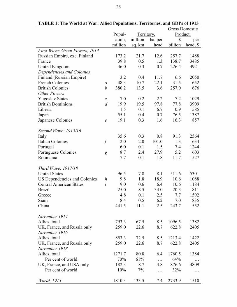
Table 1 adds up the resources on the Allied side at the outbreak of war and shows

how the volume of resources on each side changed or, more accurately, would have

changed if the populations of 1913 had remained in the same place and continued to

produce at the same rate in subsequent years as in 1913. Thus, the figures for

population and output that are reported for each territory listed in the table are those

for 1913. In reality, the populations and productivities of each territory changed year

by year as the war progressed. But we have such wartime figures only for a handful of

countries. To extend coverage to all the powers and their colonies and dependencies

as well, while maintaining comparability, it is necessary to confine ourselves to what

we know for most of the countries, that is, the situation as it was in 1913 and as it

would have been in subsequent years, had 1913 populations and productivities been

maintained.

In this table and the next, countries are listed as far as possible in order of their

entry into the war. In the first phase of the war Russia, France, and the United

Kingdom were joined together as the power of the Triple Entente. They brought with

them their dependencies and colonies. Other countries joined in too: Serbia and the

other Yugoslav states, the British Dominions, Liberia, and Japan with her colonies.

During 1915/16 a second wave of countries joined the Allies: Italy, Portugal, and

Roumania. In the third wave of 1917/18 Russia dropped out but the United States

joined in, bringing its own possessions, most of Central America and Brazil. Greece,

Siam, and China also joined. By the end of this process governments representing 70

per cent of the world’s prewar population and 64 per cent of its prewar output had

declared war on the Allied side.

The bare totals on the Allied side do not give any idea of their heterogeneity. The

British empire will do for illustration since it comprised some of the richest and

poorest regions in the world. Britain itself had a prewar population of 46 million with

an average income per head of nearly $5,000 (at 1990 prices). Its colonies, excluding

the Dominions, had a prewar population of 380 millions, mostly Indians, with an

average income of less than $700. Thus a colonial population eight times that of

Britain produced a similar volume of output. Moreover this output was far less

available than Britain’s for fighting Germany for three reasons: it was hundreds or

thousands of miles away from the theatre of war, the level of development of colonial

5

government administration and financial services rendered it hard to track and control,

and most of it was already committed to the subsistence needs of the colonial

populations. In short, the mere possession of low income territories was of little value

to a great power in the war. If India helped Britain in the war it was to enable British

trade and commerce rather than because Britain could mobilise Indian resources in

any meaningful sense. And the trade that really mattered to the British economy in the

war was with rich America and Canada, not with poor India.

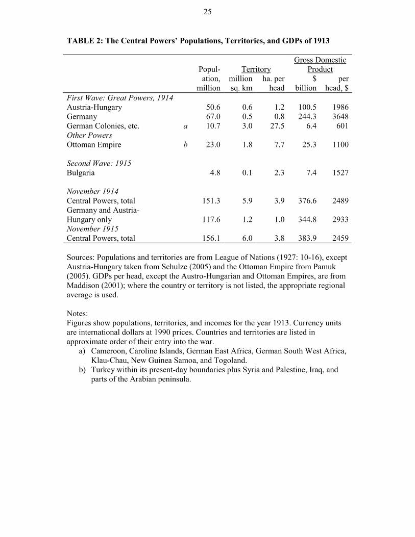
Table 2 adds up the resources of the Central Powers, using the same conventions

as Table 1. This is a much shorter story with a smaller bottom line. Austria-Hungary

began the war, joined immediately by Germany and soon by the Ottoman Empire. In

1915 the Central Powers were joined by Bulgaria, although not by Italy which went

back on its prewar treaty obligations. At its maximum extent the alliance of the

Central Powers comprised little more than 150 million people, but their relative lack

of success in accumulating low-income colonies made them relatively well off with

an average income per head of less than $2,500, roughly comparable to that of Italy

on the Allied side.

2. Allied Superiority

Table 3 allows us to compare the resources on each side at three benchmark dates:

November in each of 1914, 1916, and 1918. This table offers comparisons for each

alliance as a whole, and also counting great powers only. The rationale for the latter is

very simple: if low-income colonies did not count much, how do the figures look if

we do not count them at all? There is some imprecision here, of course. For example

Russia is included as a great power, but much of its territory was little more

developed than that of India which is excluded as a colony; also excluded are the

British Dominions, which were much richer than Russia. Still, singling out the great

powers has the merit of simplicity.

The table shows something very striking: in terms of the resources on either side

the Central Powers do not seem to have had much hope. If Germany could not win the

war for the Central Powers in the first six weeks, using surprise in the west and an

army with superior military qualities, then the chances of victory could only diminish

over a longer span of time in which economies would be mobilised on each side and

the balance of resources would count for more and more.

6

Even in the first stage of the war the Allies had access to five times the

population, eleven times the territory, and three times the output of the Central

powers.2 This access was limited by relatively low average incomes across the

colonial empires of Britain and France, and low incomes in Russia; we see that the

average level of GDP per head on the Allied side in 1914 was not much more than

half that of the Central Powers. If we consider great powers only then the Allied

advantages in population and output shrink to twice; the Allied advantage in territory

actually increases, reflecting the German and Turkish propensities to colonise sandy

deserts in Africa and the Middle East.

As the war continued, the Allied powers’ advantage in output grew. The decisive

year was 1917. When America displaced Russia the Allied population and territory

declined but its output multiplied; the average development level of the Allied powers

rose above that of the Central Powers for the first time. Although it would take time

for America’s presence to be felt on the battlefield, it sealed the Central Powers’ fate.

The force of these changes is felt even more strongly when it is remembered that

the figures in Table 3 are based on the assumption that in wartime the real output of a

given territory did not change. While we cannot track the changes for more than a few

countries, the figures available suggest further substantial swings which worked

primarily to favour the richer powers, Britain and America. Table 4 shows that in

wartime the British and American economies expanded by over 10 per cent. The trend

in Italy’s output is not really known but the Italian economy certainly kept going and

did not collapse. Russia, however, began to collapse in 1916 and France in 1917; this

emphasises the importance of the American entry into the war on the Allied side. On

the side of the Central Powers the dismal failure of wartime mobilisation was evident

from the outset: for much of the war period the German and Austrian economies

flatlined at 20 to 25 per cent below their prewar benchmarks for real output. Pamuk

(2005) estimates that by 1918 the GDP of the Ottoman Empire had declined by 30 to

40 percent.

3. The Human Factor

Where, in all this, is there room for factors other than the economic ones? Reviewing

our previous work on World War II (Harrison, 1998) the historian Richard Overy

(1998) objected that we left no role to “a whole series of contingent factors – moral,

political, technical, and organisational – [that] worked to a greater or lesser degree on

7

national war efforts.” Such factors were clearly significant in World War I, and

economists have considered why they must matter in principle (Brennan and Tullock,

1982) but we do not apologise for still giving most weight to the quantities of

resources.

At first the two sides were unequal in military and civilian organisation,

motivation, and morale. Germany entered the war with first-rate military advantages

associated with “the most formidable army in the world” (Kennedy, 1988: 341), past

victories, and the exploitation of initial shock and rapid movement, and maintained

this relative military edge throughout the war (Ferguson, 1998, 298-300). But the

effects of looming defeat electrified Britain and France, transformed public opinion,

and forced their armies and governments through intensive courses in the new rules of

warfare and mobilisation. This proved to be the pattern through the war: each

temporary setback was followed by strenuous efforts to refine strategy and strengthen

morale, organisation, and supplies, and these efforts generally succeeded within the

limits permitted by the resources available to support them. In short, the “moral,

political, technical, and organisational” issues of the war on each side were not

independently variable factors but proved to be endogenous to the progress of the war.

Other things being held equal, a deficit of organisation or morale on one side tended

to be overcome through a self-balancing process. The one thing that could not be

overcome was a deficit of resources.

This approach is well illustrated by comparing the two offensives that appeared to

give Germany its best chances of winning the war: August 1914 and March 1918. In

the first of these Germany planned to exploit mass, movement, and surprise to destroy

the French Army before the British could intervene in the West and before the

Russians could mobilise in the East. In practice the German army succeeded in many

of its planned objectives but failed in the ones that were vital. The stalemate of the

trenches resulted. Had the German plan succeeded the economic factors on each side

would never have had time to be felt. Given that it did not, the richer Allies won time

to put right their military and organisational failings, but they could not have done so

without resources on their side.

Its spring offensive in 1918 again seemed to offer Germany the prospect of

winning the war on a purely military advantage. For the first time since 1914 its

soldiers opened up great gaps in the Allied lines and advanced dozens of kilometres

towards the Channel ports. The offensive badly shocked the Allies and forced them

8

into reorganisation; the Americans had to accept a unified command. Resources

defeated the advancing Germans: their own lack of supply, for they were badly

clothed and undernourished even before they began their advance; the abundance of

supplies they found in the Allied trenches that caused many to turn away from the

attack to eat and drink their advantages away (Herwig, 1988: 102); and the

superabundance of war materials that enabled the Allies to regroup and go on to

inflict a far greater defeat on the exhausted enemy.

III. MOBILISATION AND THE LEVEL OF DEVELOPMENT

1. Four Aspects of Mobilisation

In this section we examine production mobilisation (the wartime increase in real

GDP), fiscal mobilisation (the wartime transfer of resources into the hands of

government), military mobilisation (the wartime transfer of persons into the armed

forces), and the capital-intensity of warfare (the flow ratio of weapons produced to

years of combat service). We find that the comparative success of the various

economies in mobilising their resources depended largely on their level of economic

development. In some aspects this relationship is found only after controlling for the

confounding influences of combat duration and proximity. Britain and the United

States were both rich and highly developed, for example, but the briefer involvement

of the United States in the war and its greater distance from the continental theatre of

warfare inevitably weakened some of the mobilising impulses felt there. A warning

about selection bias may also be in order: poorer countries had less good government

and national accounts, so the data reported by richer countries tends to be

overrepresented; we also have less confidence in the data of the poorer countries

when it is reported.3

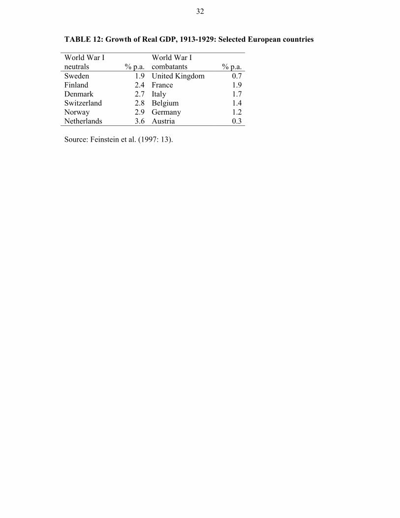
In Figure 1 production mobilisation is measured by the wartime change in GDP

up to 1917. Production mobilisation was strongly and positively correlated with

prewar GDP per head. The relationship would look still stronger if we included

Pamuk’s (2005) figures for Turkey, with a prewar GDP per head of less than $800

and a wartime output decline of 30 to 40 per cent.4

The available measures of fiscal mobilisation do not give such a clearcut result.

Figure 2, based on Table 5, shows the change in the government share of GDP in the

first year of the war for five countries close to the fighting and three distant ones. It

show a positive relationship between mobilisation and prewar development level but

9

it is necessary to control for distance for the relationship to become apparent. The

measure that we use tends to underestimate the richer countries’ ability to transfer

resources rapidly from peacetime to wartime uses since they also tended to spend a

lower proportion of their national income on defence in peacetime (Eloranta, 2003). It

is not clear whether the association suggested by Figure 2 would be strengthened by

inclusion of the Ottoman Empire where the proportion of GDP under the control of

the state was no more than 16-20 per cent at the peak (Pamuk, 2005). With regard to

fiscal mobilisation Figure 2 is our best shot: after the first year of warfare, any

relationship between fiscal mobilisation and development level ceases to be apparent.

Men and weapons may provide more unambiguous measures of mobilisation than

money. In the mobilisation of young men we find a pattern that again rises with

development and falls with distance. Figure 3 plots the wartime mobilisation rates of

various countries against their prewar incomes per head in three distance bands. The

first band comprises the front-line Eurasian states on whose territory or borders the

war was fought. The second band is for the European countries separated from the

war by land or sea, with only two members: Britain and Portugal. The third band

includes countries that joined the war from continents beyond Europe and the Near

East. Cumulative numbers mobilised are shown as a proportion of young men in the

age group from 15 to 49 years of age. In each distance band, i.e. controlling for

distance, the figures show a consistent positive dependence of the proportion

mobilised in each country on its prewar income level. However, dropping a band

lowered the proportion substantially.5

The richer countries were not only able to mobilise more men. Regardless of

distance, they also supplied them better. Capital-abundant economies were able to

support capital-intensive warfare. Figure 4 plots cumulative war production of rifles,

machine guns, field guns, tanks, and aircraft in units per thousand men mobilised

through the war and per year of the war. In each case we see that supply rose strongly

with the development level of the country.

To summarise, size mattered for the ability of a country to supply the means of

military power, but the level of economic development was a multiplier of size.

Richer countries were able to mobilise production, public finance, soldiers, and

weapons per soldier, out of proportion to their general economic capacities.

10

2. Mobilisation and Agriculture

Countries like Russia and Austria-Hungary were large; why did it make such a

difference that they were also poor? We could imagine the relationship between

mobilisation and economic development operating through several possible channels.

A pure income effect is one candidate. Another candidate is the effect of economic

development on the general quality of legal and financial institutions, that might

support more efficient wartime administration and a wider capital market to support

wartime deficit finance. A third effect, on which we concentrate here, is the effect of

economic development on the economic structure: in World War I, poor countries ran

short of food long before they ran out of guns and shells (Offer, 1989), and we

associate this with a negative influence of peasant agriculture on mobilisation.

One of the most striking attributes of relative poverty was the role of subsistence

farming. Contemporary observers were aware of these differences and interpreted

them as follows: when war broke out, a country such as Russia would have an

immediate advantage in the fact that most of its population could feed itself;

moreover, the ability to divert food supplies from export to the home market would

actually increase Russia’s advantage. In contrast Britain would quickly starve (Gatrell

and Harrison, 1993). This diagnosis could not have been more wrong. In practice the

presence of a large peasantry proved to be a great disadvantage when it came to the

mobilisation of resources for war. Peasant agriculture behaved very much like a

neutral trading partner. Why should Netherlands trade with Germany given the latter’s

reduced ability to pay, except under threat of invasion and confiscation? Peasant

farmers made the same calculation. Thus the Russian economy looked large, but if the

observers of the time had first subtracted its peasant population and farming resources

they would have seen how small and weak Russia really was. Meyendorff (cited by

Gatrell, 2005) described what happened in Russia as “the Russian peasant’s secession

from the economic fabric of the nation”. And not only from Russia, for Italy, Austria-

Hungary, the Ottoman Empire, and Germany all had large peasant populations that

proved extremely difficult to mobilise for much the same reason.

The common process of the peasant’s secession is clearly visible from a

comparison of the richer and poorer countries’ experience. When war broke out

British and American farmers boosted production because they were offered higher

prices and responded normally to incentives. The fact that British farming had already

contracted to a small part of the economy made its expansion easier: there were

11

plentiful reserves of land unused or little exploited, and the high productivity of farm

labour meant that substantial increases in farm output could be achieved with

relatively little extra in the way of resources.

In the poorer countries, in contrast, wartime mobilisation began by taking

resources away from farming, particularly young men and horses for the army. Once

in the army these young men and horses still needed to be fed, of course, which

implied a diversion of food supplies from rural households to government purchasers.

But at the same time the motivation for farmers in the countryside to sell food was

greatly reduced. These were subsistence farmers who grew food partly for their own

consumption; what they sold, they took to the market primarily to buy the

manufactured commodities, mainly textiles and metal goods, that they needed for

their families. But war dried up the supply of manufactures to the countryside. The

small industrial sectors of the poorer countries were soon wholly concentrated on

supplying the army with weapons and equipment, uniforms and rations. There was no

capacity left to supply the countryside, which faced a steep decline in supplies.

Consequently, peasant farmers retreated into subsistence activities. As the market

supply of food dried up, in the towns food prices soared.

The economy began literally to disintegrate: there might still be plenty of food,

but it was in the wrong place. The farmers preferred to eat it themselves than sell it for

a low return. The government had to feed the army at all costs for a simple reason:

hungry soldiers will not fight. Between the army and the peasantry the urban workers

were now caught in a double squeeze. There was still enough food for everyone to

have enough to eat; the localised shortages that began to spread were famines that

arose from the urban society’s loss of entitlement (Sen, 1983; Offer, 1989), not from

the decline in aggregate availability.

Aware of the unequal distribution of food, public opinion might blame unpatriotic

speculators or incompetent officials, but the truth was that a poor country had few real

choices. The scope for policy to improve the situation was usually more apparent than

real, and government action typically made things worse: for example the Russian,

Austrian, and German governments all began to ration food to the urban population,

while attempting to buy up food from the countryside at purchasing prices that were

fixed low for budgetary reasons. To repeat: in richer countries the government paid

more to the food producers, and this worked, but in poorer countries we will see that

12

the government wanted to pay less and this had entirely predictable results. The

willingness of farmers to participate in the market was still further undermined.

This process may be illustrated in a couple of diagrams. Figure 5 represents the

urban-rural markets of two countries, one that we will style “Russia” and the other

“Germany”; the difference between the two is that before 1914 Russia was a

substantial net exporter of food, Germany a net importer. The figures use the offer

curves that are conventionally used in international economics, but the market here is

partly domestic in peacetime, and wholly domestic after the war virtually halted

international trade. In both countries the farmers offer food along a curve FF and buy

manufactures along the matching curve MM but in peacetime foreign buyers and

sellers also intervene at the world terms of trade, T. Thus, in Panel A Russian farmers

sell their food surplus partly at home, partly abroad; manufactured goods are offered

partly by domestic industry along the MM curve and, when domestic marginal costs

rise above the world price, by foreigners. A corresponding role is played in Panel B

by German industry, which sells partly at home and partly abroad, importing food

when marginal costs along the domestic FF offer curve rise above the world price.

The upshot is that in both panels the rural offer is A at the world price T, while the

urban offer is B, the difference being made up by exports and imports.

By implication, when the war cuts off foreign markets, the domestic equilibrium

goes to C. The main adjustment is a fall in the availability of manufactures in Russia,

where the terms of trade shift against the peasant. In Germany it is mainly food that

becomes less available and the terms of trade facing the peasant improve. This is not

the end of the story, however.

Figure 6 shows further effects of war on the market equilibrium. The military

mobilisation of young men, horses, and nitrates raised farm costs. Nitrates proved to

be a classic “dual use” commodity of modern warfare. They were an essential

ingredient in both farm fertilisers and high explosives. Their chemical instability

made them very hard to synthesise. Before World War I the bulk supply of nitrates to

Europe came from natural deposits overseas. The trade disruption associated with the

war forced the development of a German industry to manufacture nitrates artificially,

but these were costly and war needs took up the supply that was created (Lee, 1975).

As a result the availability of nitrates for farming fell sharply in Germany, but the

impact was less in Russia where the initial reliance on nitrates was less widespread.

The losses of human, animal, and chemical power combined to push the rural offer

13

curve leftward to FF′ in both countries. This shift was limited, however, by the fact

that young men and horses are consumers of food as well as producers. At the same

time a decline in the availability of manufactures for rural consumption displaced the

urban offer curve sharply downwards to MM′. In Panel A we suppose for illustration

that the MM downshift exceeded the leftward shift of FF because limited industrial

capacity was greatly pre-empted by wartime mobilisation. A great market contraction

followed, equilibrium adjustment leading both countries to D. In Germany the

notional improvement in the peasants’ terms of trade from economic isolation was

counter-balanced by further movement to T′. In Russia the peasants’ terms of trade

became doubly disadvantageous.

Finally, the government stepped in and tried to hold food prices down by

enforcing a state price at T′′, creating excess demand and scope for a black market in

each country. This is shown in Figure 6, Panel B. To the extent that such controls

were effective, the rural offer fell back to E although urban agents were willing to

trade at G at the state enforced terms of trade. The EG gap reflected a matching

unsatisfied demand for food and an excess supply of manufactures: the least

privileged townspeople would be found in the markets trying to sell off their

fabricated possessions for money that farmers would refuse to accept for their

produce. To the extent that intervention failed, however, there was scope for black

marketeers to step in and capture rents; as long as the rents were competed away

production and consumption could both tend back to D but popular respect for law

and government would inevitably suffer in the process.

Here we see why the outcome was potentially as bad for German consumers as for

Russians, or worse. The Russians did indeed have their prewar export surplus to fall

back on. Although a much richer nation than Russia, urban famine was as acute in

Germany in the closing stages of the war.

Some readers may be surprised to find Germany numbered among the countries

that suffered a decline in agricultural output during the war. Although pre-1914

Germany has entered the economic history textbooks as a developed economic power,

it should be noted that its modernisation was highly unbalanced. High levels of

productivity in heavy industry co-existed with much lower productivity in light

industry, and much of the service sector was also characterised by low productivity,

despite Gerschenkron’s (1962) focus on the modernised railways and the universal

banks (Broadberry, 1998). But perhaps the most obvious sign of Germany’s relative

14

backwardness was the high share of the labour force engaged in low productivity

agriculture. Germany paid a high price during the two world wars for protecting its

agriculture in peacetime (Olson, 1963).

In summary, to be poor when war broke out was to suffer the consequences of a

peasant agriculture, which was essentially a dead weight on the mobilisation efforts of

the country concerned. For this purpose we include Germany. The process that

resulted had its inexorable conclusion in urban famine, revolutionary insurrection, and

the downfall of emperors.

IV. EFFECTS OF THE WAR ON THE ECONOMY

We begin our analysis of the effects of the war on the economy by considering the

scale of the destruction of physical and human capital. This forces us to reconsider the

literature produced during the immediate aftermath of the war on the direct and

indirect costs of war, which we reinterpret in the context of a national balance sheet

approach. We then consider the effects on economic growth of this capital

destruction. Comparing 1929 with 1918, it is clear that the economies which suffered

the worst destruction during the war experienced the fastest growth during the 1920s,

as would be predicted in a neoclassical growth model with a declining marginal

product of capital. However, comparing 1929 with 1913, it is equally clear that the

war lowered the growth rate of per capita income for Europe as a whole, and

particularly for combatant countries relative to neutral countries. Europe remained on

this slow growth path until after World War II, with the higher growth rate between

1950 and 1973 merely returning the European economy to its pre-1914 trend

projected forward in time.

1. Bogart’s Study of Direct and Indirect Costs

Table 6 provides estimates of what Bogart (1920) labels “direct costs” of the war.

These costs are calculated as the flow of spending by governments on the prosecution

of the war, i.e. spending over and above normal prewar levels. Inter-allied transfers

are subtracted from gross expenditures to arrive at net costs, which show the heaviest

burden to have been borne by Britain and Germany, with France, Russia and the

United States also bearing a substantial net cost on the Allied side and Austria-

Hungary amongst the Central Powers. On a per capita basis, Britain, France and

Germany stand out as bearing a much higher net cost than the other countries.

Nevertheless there are a number of disadvantages to the way that Bogart presents the

15

data. First, it is inappropriate simply to add up nominal sums spent at different times,

given the wartime inflation. Second, this problem, as well as the related problem of

the conversion to dollars of all values expressed in national currencies can be avoided

if the war expenditures are expressed as a proportion of national income in each year,

as in Table 5 above.

Table 7 introduces a number of what Bogart labels “indirect costs”, consisting

largely of losses to human and physical capital. The capitalised value of war deaths

shows the biggest losses to have been sustained by Russia and Germany, with other

substantial losses borne by Britain, France and Austria-Hungary. Property losses on

land were heaviest in France and Belgium, which is included here in Other Allies. The

heaviest shipping losses were sustained by Britain, the dominant nation in world

shipping before 1914.

A number of accounting procedures here give cause for concern. Although the

accounting for losses to physical capital is unremarkable (remembering that cargoes

can be seen as inventories), the treatment of human capital requires some attention.

The capitalised value of human life, based simply on lifetime earnings, would

overstate the social loss since people consume as well as produce. One way of

arriving at the social loss is therefore to subtract consumption from lifetime earnings,

as in the work of Clark (1931). Obviously this is not an attempt to capture the loss of

utility arising from war deaths, but merely treats people as human capital to be

replaced like physical capital so as to maintain production. As Edelstein (2000: 349)

points out “It is absurd to think the methods and perspectives of economic history can

come anywhere near to comprehending the meaning of human losses from war. We

are far better served by the speeches and letters of Lincoln or the poetry of Sassoon,

Brooke, Owen, Graves and Seager.” However, for symmetry with the treatment of

physical capital on a replacement cost basis, the simplest procedure is to add up the

cost of rearing and training a worker, since this is the net loss to society by premature

death.

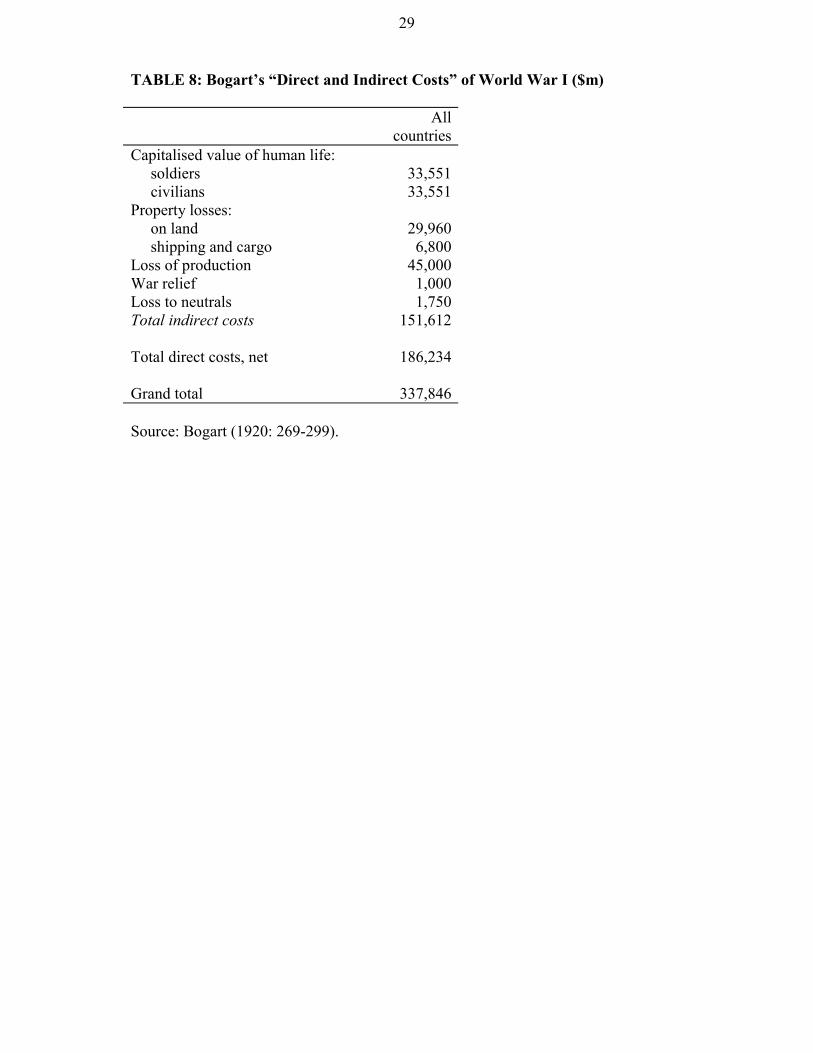
In Table 8, Bogart simply adds the direct and indirect costs to arrive at a grand

total. The justification for this is unclear, since it combines flows of current spending

with changes in the stock of assets needed to generate those flows. To add to the

confusion, lost production (a flow concept) is included as an indirect cost (a stock

concept). Note also that some of the government spending on the war effort, which is

included negatively as a direct cost by Bogart, should actually enter positively in the

16

national balance sheet, contributing to intangible physical and human capital. To the

extent that the war induced additional spending on health and welfare, this contributed

to the accumulation of intangible human capital, while research expenditure on the

development of weapons may have had spin-off effects on the accumulation of

intangible physical capital. Finally, note that Bogart (1920: 299) makes no attempt to

relate his estimates of the direct and indirect costs of World War I to levels of income

or wealth, but simply concludes that “the figures presented in this summary are both

incomprehensible and appalling”. This is an issue which can be addressed in the

national balance sheet approach.

2. Effects on National Balance Sheets

Broadberry and Howlett (1998) provide an accounting framework for evaluating the

long run impact of war on wealth, which is based on national balance sheets. The first

important distinction is between stocks and flows in the system of national accounts.

Issues concerned with the scale of mobilisation are best tackled by looking at flows of

income, expenditure and output, and calculating the proportion of these flows that is

devoted to the war effort, as in Table 5. However, the long run impact of the war can

best be assessed by looking at the effects on national wealth, defined here to include

human as well as physical capital, intangible as well as tangible capital and net

overseas assets (Goldsmith et al., 1963; Revell, 1967; Kendrick, 1976).

Tangible physical capital is the conventional form of capital, consisting of

buildings, equipment and inventories. Intangible physical capital is cumulated

expenditure on research and development, which is seen as improving the quality of

the tangible physical capital. Tangible human capital is the spending required to

produce an uneducated, untrained worker, i.e. basic rearing costs. Intangible human

capital is mainly spending on education and training to improve the quality of the

human capital, although it also includes other items such as spending on health and

safety and mobility costs. In an open economy, the impact of the war on net overseas

assets must also be taken into account.

We believe that this accounting framework deals with the main objections

raised by writers such as Hardach (1977: 286) and Milward (1984: 9-27) to previous

attempts to quantify the impact of war on the economy. In particular, note that: (1) a

clear distinction between stock and flow concepts is maintained throughout (2) all

nominal values are converted to a constant price basis so that values for different

17

years can be added together (3) human capital calculations take account of the fact

that people consume as well as produce (4) the fact that postwar birth rates rise does

not alter the fact that the human capital embodied in those killed by warfare is lost;

this has a negative impact on national wealth as much as any destruction of physical

capital, which is usually followed by increased investment to make good war losses

(5) technological change stimulated by wartime research and development can be

seen as having a positive impact on intangible physical capital (6) social spending

stimulated by the war can be seen as having a positive impact on intangible human

capital.

3. War Casualties and Human Capital Losses

One obvious cost of the war was the huge number of deaths resulting from the

“industrialisation” of warfare, which led to the growing use of the term “total war”

(Chickering and Förster, 2000). There are conceptual difficulties with the types of

death to be included in any definition of war deaths, which could be restricted to

battle deaths of military personnel or broadened to include non-battle deaths of

civilians as well as military personnel. We have opted for battle and non-battle deaths

of military personnel, following Urlanis (1971) since this offers a high degree of

uniformity in data across countries while going beyond those killed in battle or who

died from wounds or poison gas. Non-battle deaths includes those who died from

disease, died in captivity or died from accidents and other causes. We exclude most

deaths in the influenza pandemic of 1918, however.

The data in Table 9 show how military deaths were spread across the

combatant countries. Germany suffered the most casualties in absolute numbers,

although a number of countries sustained heavier losses as a percentage of the

population, including France, Serbia-Montenegro and Rumania amongst the Allies

and Turkey amongst the Central Powers. Although Russia sustained the second

highest losses in absolute numbers, this was a lower proportion of the population than

the losses in Britain and Italy amongst the Allies and Austria-Hungary amongst the

Central Powers. Taking the Central Powers and the Allies together, the battle and

non-battle deaths of military personnel represented about 1% of the population of the

combatant nations.

Turning these casualties into estimates of human capital losses in the national

balance sheet framework requires knowledge of the prewar costs of rearing and

18

educating a child, together with cohort-specific estimates of the education of the

labour force. In the absence of sufficient data for many countries, the human capital

losses in Table 10 are calculated as the ratio of war deaths to the prewar population of

prime working age, taken from Urlanis (1971). This differs from the proportion of

human capital destroyed by the war to the extent that younger cohorts had more

human capital investment, particularly through education. Also, since the human

capital losses are not calculated in monetary units, they cannot be added to physical

capital losses to provide an estimate of the proportion of physical and human capital

destroyed by the war.

4. Physical Capital Losses and Changing National Wealth

Turning to physical capital losses in Table 10, we have largely relied for the losses of

domestic assets on Bogart’s (1920) estimates of property losses on land and shipping

and cargo losses from Table 7. However, whereas Bogart (1920) expressed the losses

in terms of US dollars, we have expressed them as percentages of prewar capital.

France’s losses were extremely heavy when expressed as a percentage of prewar

capital in Table 10, as well as in dollar terms in Table 7.6 Russia’s losses appear rather

heavier in proportionate terms than in absolute dollar values, due to the low level of

Russia’s prewar capital stock. Also in Table 10, for some countries it has been

possible to obtain estimates of the change in overseas assets and national wealth. In

the case of Britain, nearly a quarter of overseas investments were liquidated during

the war, so that the reduction of national wealth was proportionally much greater than

the loss of physical capital. For France, although the loss of overseas assets was

proportionally higher due to heavy exposure to Russian loans, the share of physical

capital losses was also much higher than in Britain (Hardach, 1977: 289-290). Hence

the share of national wealth lost in the war was about the same as the share of

physical capital lost.

In principle, some of the government spending on the war effort, which is

included negatively as a direct cost by Bogart (1920) should actually enter positively

in the national balance sheet, contributing to intangible physical capital in the form of

cumulated research and development spending and to intangible human capital in the

form of spending on health and mobility. However, in practice, Broadberry and

Howlett (1998) found that these effects were very small even during World War II.

During World War I, these positive effects were difficult to discern at all in the British

19

case. Such effects were unlikely to have been of much more significance for other

countries.

5. Reparations and National Wealth

Finally in Table 10, we have added in Germany’s reparations bill as a proportion of

prewar capital, since they represented an increase in overseas liabilities and hence a

reduction in national wealth just as much as the liquidation of Britain’s overseas

assets meant a reduction in national wealth. Of course there is a huge debate over the

extent to which Germany actually had to pay these reparations, but that does not alter

the effect on the national balance sheet as it stood immediately after the Treaty of

Versailles (Ritschl, 2003). These figures include the A+B+C Bonds, which added up

to a total of 132 billion Gold Marks.

V. THE IMPACT ON GROWTH AND DEVELOPMENT

Milward (1984: 15-16) is critical of studies that focus on the costs of the war, which

he sees as neglecting the wider impact of the war on growth and development. This

reflects a substantial literature arguing that the two world wars stimulated economic

and social changes which had positive as well as negative effects (Andrzejewski,

1954; Titmuss, 1950). However, there are good grounds to be sceptical here. Milward

(1984: 17-18) cites Bowley (1930) as a pioneer of this view, but Bowley (1930: 21-

23) himself pointed out how difficult it is to show that any of these wider changes

were actually the result of the war and would not have occurred anyway in its

absence. Classifying developments as (a) mainly unconnected with the war, (b)

accelerated or retarded by it or (c) apparently arising out of it, Bowley was himself

reluctant to put anything other than the key elements of the “cost of war” calculations

such as loss of life and destruction of capital into category (c). He did mention the

new economic relation between Europe and the United States in this category, but

with hindsight we can see that the process of US overtaking was already underway

well before World War I (Abramovitz, 1986; Broadberry 1998).

1. Wartime destruction and postwar recovery

The neoclassical growth model assumes a diminishing marginal product of capital.

Hence capital destruction should lead to an increase in the marginal product of capital

and faster growth during a transitional phase. This suggestion of a negative

relationship between the scale of wartime destruction and the subsequent growth rate

20

has previously been quantified in the literature on the post-World War II period,

particularly by Janossy (1971), who used it to predict the end of the postwar economic

miracles in Germany and Japan, subsequently borne out by events (Dumke, 1990).

The relationship has been little discussed in the context of World War I, with the

notable exception of a study by Eichengreen (1990), who pointed to a negative

relationship between the growth of industrial production 1921-1927 and the level of

industrial production in 1921 relative to its 1913 level in a sample of thirteen

industrial countries.

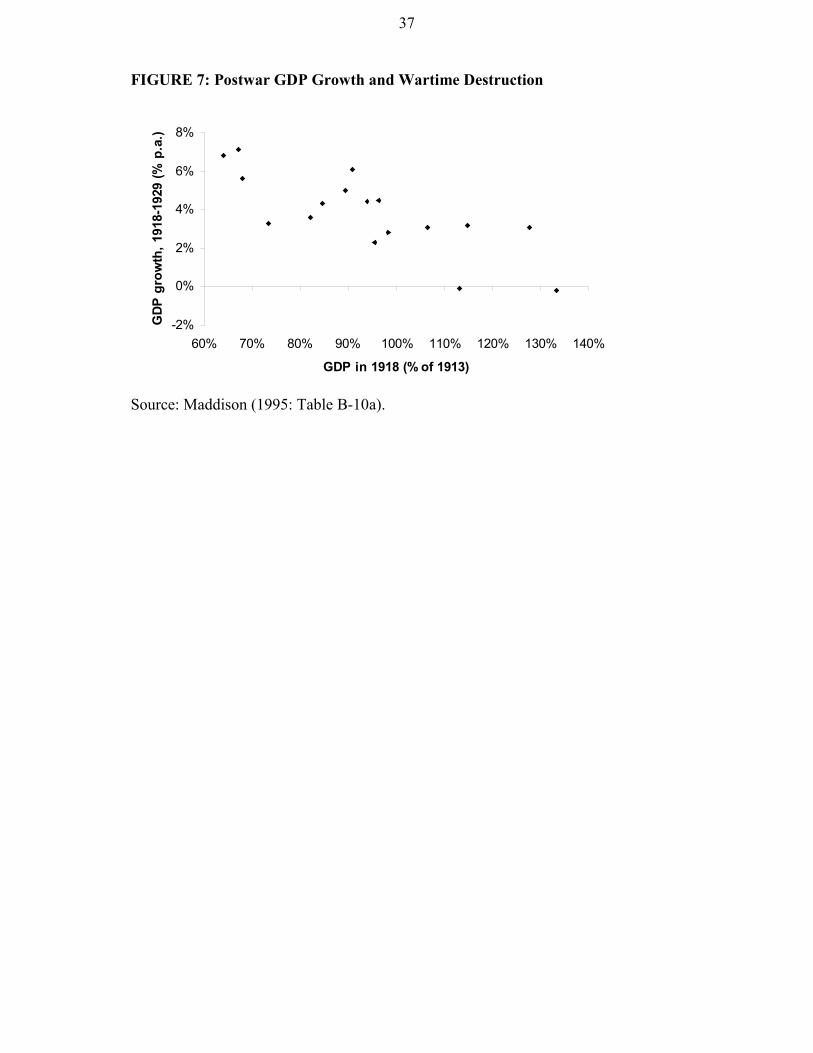
Figure 7 shows the relationship between GDP growth during the recovery

period 1918-1929 and the scale of wartime destruction as measured by the level of

GDP in 1918 relative to 1913, for a sample of 17 rich nations from Maddison (1995).

The negative relationship can be confirmed using regression analysis.7

2. Effects on growth over the longer run

Over the longer run, however, there is little doubt that World war I had a negative

impact on the growth rate in Europe as a whole. One way of understanding that is

through the effects on accumulation. As already noted, the war had a significant

negative impact on physical and human capital in the combatant countries. Although

there was some rebound, it was not sufficient to undo the damage of the war.

Furthermore, these negative effects on accumulation had a high degree of persistence

because of the effects of the war on the institutional framework. Although World War

I may be seen as the culmination of a period of existing national rivalry, there can be

little doubt that it served to strengthen the forces of nationalism. This can be seen as

having serious economic consequences, giving a boost to protectionism and autarkic

policies during the 1920s and 1930s.

The consequences of the capital destruction of the war combined with the

economic dislocation of its aftermath for the growth of per capita income in Europe

and other parts of the world over the longer run can be seen in Table 11. The first

point to note is that growth of per capita GDP for a weighted average of fifteen

European countries was 1.8 per cent per annum between 1890 and 1994. However,

whilst Europe grew at roughly this secular rate before 1914 and after 1973, there was

a period of slower growth between 1913 and 1950, followed by a period of more rapid

growth between 1950 and 1973. This slower growth during 1913-1950 is interpreted

by Feinstein et al. (1997:8-9) as the destructive impact of World War I, followed by

21

the economic disintegration of the interwar period and the further destruction of

World War II. The argument is given added weight by the fact that the impact was

much greater in Europe than in the United States, since the war was fought largely on

European soil with unprecedented severity, and Europe’s economies were more

dependent on international economic transactions before 1914. On this interpretation,

the period 1950-1973 is best seen as catching-up in a more integrated world economy.

Turning in Table 12 to variation between European countries in the growth

rate of GDP during the shorter period 1913-1929, we see that the most important

difference is between neutral and combatant countries. The lowest growth rate

amongst the neutrals (Sweden) was equal to the highest growth rate amongst the

combatants (France). This again supports the emphasis on the costs of war in the

traditional literature. Important themes stressed in this literature include the

protectionist environment and the general lack of international co-operation over the

international monetary system as well as the international trading system

(Eichengreen, 1992). One factor which needs to be mentioned here is the proliferation

of independent nation states following the break-up of the Austro-Hungarian and

Ottoman Empires. This was based on one of the founding principles of the League of

Nations, the self-determination of nations. In eastern and central Europe, this led to a

proliferation of states with separate currencies and customs jurisdictions. In a less

protectionist environment, this may not have been of great significance, but in the

context of protectionist interwar Europe, it clearly had serious trade-diverting effects.

Nevertheless, although there was clearly a net effect of economic disintegration in

central and eastern Europe, we should not forget that there were also areas of

increased integration. Probably of most significance here was the increased

integration of the reunited parts of Poland that had previously been partitioned

between Prussia, Austria and Russia (Wolf, 2003).

V. CONCLUSIONS

We have used the experience of the major combatant countries in World War I to

analyse the role of economic factors in determining the outcome of the war and the

effects of the war on subsequent economic performance. We have shown, first, that

the degree of mobilisation for war can be explained largely by differences in the level

of development of each country, leaving little room for other factors that feature

prominently in narrative accounts, such as national differences in war preparations,

22

war leadership, military organisation and morale. This matches the conclusions of

Harrison (1998) that the outcome of World War II was also determined largely by

economic factors. For total warfare during the twentieth century, at least, it seems that

the outcome of wars can be explained quite simply: in the words of James Carville,

managing Bill Clinton’s US presidential election campaign in 1992, “It’s the

economy. Stupid”.

We have examined the effects of the war on subsequent economic

performance in terms of the scale of destruction of physical and human capital. Here,

we defend the basic approach of liberal economists who calculated the costs of the

war, but we reinterpret the results within a national balance sheet framework.

Although the growth rate between 1918 and 1929 was highest in the economies which

experienced the worst destruction, over the period 1913-1929 as a whole, per capita

income growth in Europe was reduced. Thus there was some rebound, but not enough

to undo the negative effects of the capital destruction and the damage to the

international institutional framework caused by the war.

23

TABLE 1: The World at War: Allied Populations, Territories, and GDPs of 1913

Territory,Gross Domestic

Product,Popul-ation,

millionmillionsq. km

ha. perhead

$billion

perhead, $

First Wave: Great Powers, 1914Russian Empire, exc. Finland 173.2 21.7 12.6 257.7 1488France 39.8 0.5 1.3 138.7 3485United Kingdom 46.0 0.3 0.7 226.4 4921Dependencies and ColoniesFinland (Russian Empire) 3.2 0.4 11.7 6.6 2050French Colonies a 48.3 10.7 22.1 31.5 652British Colonies b 380.2 13.5 3.6 257.0 676Other PowersYugoslav States c 7.0 0.2 2.2 7.2 1029British Dominions d 19.9 19.5 97.8 77.8 3909Liberia 1.5 0.1 6.7 0.9 585Japan 55.1 0.4 0.7 76.5 1387Japanese Colonies e 19.1 0.3 1.6 16.3 857

Second Wave: 1915/16Italy 35.6 0.3 0.8 91.3 2564Italian Colonies f 2.0 2.0 101.0 1.3 634Portugal 6.0 0.1 1.5 7.4 1244Portuguese Colonies g 8.7 2.4 27.9 5.2 603Roumania 7.7 0.1 1.8 11.7 1527

Third Wave: 1917/18United States 96.5 7.8 8.1 511.6 5301US Dependencies and Colonies h 9.8 1.8 18.9 10.6 1088Central American States i 9.0 0.6 6.4 10.6 1184Brazil 25.0 8.5 34.0 20.3 811Greece 4.8 0.1 2.5 7.7 1592Siam 8.4 0.5 6.2 7.0 835China 441.5 11.1 2.5 243.7 552

November 1914Allies, total 793.3 67.5 8.5 1096.5 1382UK, France, and Russia only 259.0 22.6 8.7 622.8 2405November 1916Allies, total 853.3 72.5 8.5 1213.4 1422UK, France, and Russia only 259.0 22.6 8.7 622.8 2405November 1918Allies, total 1271.7 80.8 6.4 1760.5 1384

Per cent of world 70% 61% … 64% …UK, France, and USA only 182.3 8.7 4.8 876.6 4809

Per cent of world 10% 7% … 32% …

World, 1913 1810.3 133.5 7.4 2733.9 1510

24

Sources: Populations and territories are from League of Nations (1927: 10-16). GDPsper head are from Maddison (2001); where the country or territory is not listed, theappropriate regional average is used.Notes: Figures show populations, territories, and incomes for the year 1913. Currencyunits are international dollars at 1990 prices. Countries and territories are listed inapproximate order of their entry into the war.

a) Many countries in Africa, Asia, and Oceania. Algeria, French West Africa,and Indo-China together accounted for more than 70% of the population andGDP but less than half of the territory of the French Empire.

b) Many countries in Africa, Asia, and Oceania, including Anglo-French andAnglo-Egyptian territories. India accounted for more than four fifths of thepopulation and GDP but only one third of the territory of the British Empirenot counting the Dominions.

c) Serbia, Bosnia-Herzegovina, and Montenegro.d) Australia, Canada (including Labrador and Newfoundland), New Zealand, and

Union of South Africa.e) Korea, Formosa, Kwantung, and Sakhalin.f) Eritrea, Libya, Somalia, the Aegean Islands, and Tientsin.g) Angola, Cape Verde Islands, Portuguese Guinea, Mozambique, St Thome and

Principe Islands, Portuguese India, Macao, and Timor and Cambing.h) Alaska, American Samoa, Guam, Hawaii, the Panama Canal Zone, and

Phillipines.i) Costa Rica, Cuba, Guatemala, Haiti, Honduras, Nicaragua, and Panama.

25

TABLE 2: The Central Powers’ Populations, Territories, and GDPs of 1913

TerritoryGross Domestic

ProductPopul-ation,

millionmillionsq. km

ha. perhead

$billion

perhead, $

First Wave: Great Powers, 1914Austria-Hungary 50.6 0.6 1.2 100.5 1986Germany 67.0 0.5 0.8 244.3 3648German Colonies, etc. a 10.7 3.0 27.5 6.4 601Other PowersOttoman Empire b 23.0 1.8 7.7 25.3 1100

Second Wave: 1915Bulgaria 4.8 0.1 2.3 7.4 1527

November 1914Central Powers, total 151.3 5.9 3.9 376.6 2489Germany and Austria-Hungary only 117.6 1.2 1.0 344.8 2933November 1915Central Powers, total 156.1 6.0 3.8 383.9 2459

Sources: Populations and territories are from League of Nations (1927: 10-16), exceptAustria-Hungary taken from Schulze (2005) and the Ottoman Empire from Pamuk(2005). GDPs per head, except the Austro-Hungarian and Ottoman Empires, are fromMaddison (2001); where the country or territory is not listed, the appropriate regionalaverage is used.

Notes:Figures show populations, territories, and incomes for the year 1913. Currency unitsare international dollars at 1990 prices. Countries and territories are listed inapproximate order of their entry into the war.

a) Cameroon, Caroline Islands, German East Africa, German South West Africa,Klau-Chau, New Guinea Samoa, and Togoland.

b) Turkey within its present-day boundaries plus Syria and Palestine, Iraq, andparts of the Arabian peninsula.

26

TABLE 3: Allies Versus Central Powers: Resource and Development Ratios

Population TerritoryTerritoryper head

GrossDomestic

ProductGDP per

headNovember 1914Total 5.2 11.5 2.2 2.9 0.6Great Powers only 2.2 19.4 8.8 1.8 0.8

November 1916Total 5.5 12.1 2.2 3.2 0.6Great Powers only 2.2 19.4 8.8 1.8 0.8

November 1918Total 8.1 13.5 1.7 4.6 0.6Great Powers only 1.6 7.5 4.8 2.5 1.6

Source: Calculated from Tables 1 and 2. Figures show ratios of Allies (Table 1) toCentral Powers (Table 2) in populations, territories, and incomes for the year 1913.Currency units are international dollars at 1990 prices.

TABLE 4: The Wartime Change in Real GDP: 1914-1918, by Country

UK USA Germany Austria Russia France1913 100 100 100 100 100 1001914 92.3 101.0 85.2 83.5 94.5 92.91915 94.9 109.1 80.9 77.4 95.5 91.01916 108.0 111.5 81.7 76.5 79.8 95.61917 105.3 112.5 81.8 74.8 67.7 81.01918 114.8 113.2 81.8 73.3 … 63.9

Sources: Maddison (1995: 148-51), except Russia from Gatrell (2005). Italy isomitted for reasons given in Broadberry (2005).

27

TABLE 5: The Share of Government Spending in National Income: 1913-1918,by Country (per cent of GDP at current prices)

Australia Canada France Germany UK USA1913 5.5 7.0 10.0 9.8 8.1 1.81914 5.7 10.0 22.3 23.9 12.7 1.91915 9.6 13.1 46.4 43.8 33.3 1.91916 14.0 16.5 47.2 50.3 37.1 1.51917 17.2 15.7 49.9 59.0 37.1 3.21918 17.2 16.9 53.5 50.1 35.1 16.6

Sources: Obstfeld and Taylor (2003); Mitchell (2003a, 2003b); France fromHautcoeur (2005); Germany from Sommariva and Tullio (1987); and UK fromFeinstein (1972: tables 2 and 3). Thanks to Jari Eloranta for help with these figures.

28

TABLE 6: Bogart’s “Direct Costs” of World War I

Gross cost($m)

Advances toallies ($m)

Net cost($m)

Net cost percapita ($)

Great Britain 44,029 8,695 35,334 766Rest of British Empire 4,494 4,494 13France 25,813 1,547 24,266 613Russia 22,594 22,594 135Italy 12,314 12,314 343United States 32,080 9,455 22,625 229Other Allies 3,964 3,964 127Total Allies 145,288 19,697 125,591

Germany 40,150 2,375 37,775 557Austria-Hungary 20,623 20,623 352Turkey and Bulgaria 2,245 2,245 85Total Central Powers 63,018 2,375 60,643

Total 208,306 22,072 186,234

Sources: Cost data from Bogart (1920: 267); Population data from Urlanis (1971:209).

TABLE 7: Bogart’s “Indirect Costs” of World War I ($m)

Capitalisedvalue of

war deaths

Propertylosses on

land

Shippingand cargo

lossesBritish Empire 3,477 1,750 3,930France 4,818 10,000 453Russia 8,104 1,250 933Italy 2,385 2,710 431United States 518 365Other Allies 3,215 11,500 525Total Allies 22,517 27,210 6,637

Germany 6,751 1,750 121Austria-Hungary 3,080 1,000 15Turkey and Bulgaria 1,203 27Total Central Powers 11,034 2,750 163

Total 33,551 29,960 6,800

Source: Bogart (1920: 269-299).Notes: For shipping losses, Other Entente Allies includes neutrals.

29

TABLE 8: Bogart’s “Direct and Indirect Costs” of World War I ($m)

Allcountries

Capitalised value of human life: soldiers 33,551 civilians 33,551Property losses: on land 29,960 shipping and cargo 6,800Loss of production 45,000War relief 1,000Loss to neutrals 1,750Total indirect costs 151,612

Total direct costs, net 186,234

Grand total 337,846

Source: Bogart (1920: 269-299).

30

TABLE 9: Battle and Non-Battle Deaths of Military Personnel in World War I

Deaths(1000s)

Population(millions)

Deaths as %of population

Great Britain 715 46.1 1.6British Empire 198 342.2 0.1France 1,327 39.6 3.4French colonies 71 52.7 0.1Russia 1,811 167.0 1.1Italy 578 35.9 1.6USA 114 98.8 0.1Belgium 38 7.6 0.5Serbia-Montenegro 278 4.9 5.7Rumania 250 7.6 3.3Greece 26 4.9 0.5Portugal 7 6.1 0.1Total Allies 5,413 813.4 0.7

Germany 2,037 67.8 3.0Austria-Hungary 1,100 58.6 1.9Turkey 804 21.7 3.7Bulgaria 88 4.7 1.9Total Central Powers 4,029 152.8 2.6

Total 9,442 966.2 1.0

Source: Urlanis (1971: 209).Notes: Battle deaths includes killed in battle, died from wounds and died from poisongas. Non-battle deaths includes died from disease, died in captivity and died fromaccidents and other causes.

31

TABLE 10: Destruction of Human and Physical Capital (% of prewar assets)

Physical capitalHumancapital

Domesticassets

Overseasassets

Reparationsbill

Nationalwealth

AlliesBritain 3.6 9.9 23.9 … 14.9France 7.2 59.6 49.0 … 54.7Russia 2.3 14.3 … … ...Italy 3.8 15.9 … … …United States 0.3 … … … …Central PowersGermany 6.3 3.1 … 51.6 54.7Austria-Hungary 4.5 6.5 … … …Turkey and Bulgaria 6.8 … … … …

Sources: Human capital: war deaths as a percentage of population aged 15-49 fromUrlanis (1971: 209). Physical capital: Britain: Broadberry and Howlett (2005);France: Hautcoeur (2005) and Hardach (1977: 289-290); Russia: Gatrell (2005); Italy:Property and shipping losses from Bogart (1920), capital from Ercolani (1969);Germany: Property and shipping losses from Bogart (1920), capital from Hoffmann(1965), with reparations bill from Hardach (1977: 248); Austria-Hungary: Propertylosses from Bogart (1920), capital from Fellner (1915).Notes: Reparations bill expressed as % of prewar physical capital.

TABLE 11: Growth of Real GDP, 1890-1994: Europe and the United States (percent per year, average)

EuropeGDP population GDP per

head

USA,GDP per

head1890-1994 2.4 0.6 1.8 1.81890-1913 2.2 0.7 1.4 2.01913-1950 1.4 0.5 0.9 1.41950-1973 4.8 0.8 4.0 2.91973-1994 2.1 0.4 1.7 1.4

Source: Feinstein et al. (1997: 7, 9).

32

TABLE 12: Growth of Real GDP, 1913-1929: Selected European countries

World War Ineutrals % p.a.

World War Icombatants % p.a.

Sweden 1.9 United Kingdom 0.7Finland 2.4 France 1.9Denmark 2.7 Italy 1.7Switzerland 2.8 Belgium 1.4Norway 2.9 Germany 1.2Netherlands 3.6 Austria 0.3

Source: Feinstein et al. (1997: 13).

33

FIGURE 1: Production Mobilisation, 1913 to 1917: Ten Countries

-40%

-20%

0%

20%

40%

0 1000 2000 3000 4000 5000 6000

GDP per Head in 1913, $ and 1990 prices

Cha

nge

in R

eal G

DP

1913

to

1917

Source: Table 4 and Maddison (2001). Observations from left to right are Russia,Austria-Hungary, France, Germany, Canada, UK, New Zealand, USA, and Australia.Territories are measured within contemporary frontiers. Currency units areinternational dollars at 1990 prices.

FIGURE 2: Fiscal Mobilisation in the First Year of War: Eight Countries

-10%

0%

10%

20%

30%

0 1000 2000 3000 4000 5000 6000

GDP Per Head in 1913, $ and 1990 Prices

Ch

ang

e in

Gov

ern

men

t O

utl

ays,

S

har

e of

GD

P,

Firs

t Y

ear

of W

ar

Canada Australia

USA

Source: Table 5, except Austria-Hungary (military expenditure only) from Schulze(2005). Observations not labelled within the figure are, from left to right, Austria-Hungary, Italy, France, Germany, and UK.

34

FIGURE 3: Military Mobilisation, 1914-1918: Eighteen Countries and theFrench Colonies

0%

20%

40%

60%

80%

100%

0 1000 2000 3000 4000 5000 6000

GDP per head, $ and 1990 prices

Mob

ilisa

tio

n, p

er

cen

t o

f m

ale

s,

15-

49

Front Line Eurasia0%

20%

40%

60%

0 1000 2000 3000 4000 5000 6000

GDP per head, $ and 1990 prices

Mob

ilisa

tio

n, p

er

cen

t o

f m

ale

s,

15-

49

European Periphery

0%

20%

40%

60%

0 1000 2000 3000 4000 5000 6000

GDP per head, $ and 1990 prices

Mob

ilisa

tio

n, p

er

cen

t o

f m

ale

s,

15-

49

Non-European States

Sources: GDPs per head in 1913 from Tables 1 and 2 or, if not listed there, fromMaddison (2001: 185); cumulative mobilisation rates, 1914-1918, from Urlanis(1971: 209).Note: Observations, reading from left to right in order of increasing GDP per head areas follows. Front line Eurasia: Serbia, Turkey, Russia, Bulgaria, Roumania, Greece,Austria-Hungary, Italy, France, and Germany. European periphery: Portugal and UK.Non-European States: French colonies, India, South Africa, Canada, New Zealand,USA, Australia.

35

FIGURE 4: The Capital-Intensity of Warfare, 1914-1918: Six Countries

0

100

200

300

400

500

600

0 1000 2000 3000 4000 5000 6000

GDP per head, $ and 1990 prices

Rifl

es p

er

thou

sand

com

bata

nt-

yea

rs

0

2

4

6

8

10

12

14

0 1000 2000 3000 4000 5000 6000

GDP per head, $ and 1990 prices

Ma

chin

e g

uns

per

thou

sand

co

mba

tant

-ye

ars

0.0

0.2

0.4

0.6

0.8

1.0

1.2

0 1000 2000 3000 4000 5000 6000

GDP per head, $ and 1990 prices

Gun

s pe

r th

ousa

nd c

omba

tant

-ye

ars

0.00

0.02

0.04

0.06

0.08

0.10

0.12

0.14

0.16

0.18

0 1000 2000 3000 4000 5000 6000

GDP per head, $ and 1990 prices

Tank

s pe

r th

ousa

nd c

omba

tant

-ye

ars

0.0

0.5

1.0

1.5

2.0

2.5

0 1000 2000 3000 4000 5000 6000

GDP per head, $ and 1990 prices

Air

cra

ft p

er

thou

sand

co

mba

tant

-ye

ars

Sources: GDPs per head in 1913 from Tables 1 and 2; cumulative war production,1914-1918, from Adelman (1988: 45), except UK from Broadberry and Howlett(2005) and Austria-Hungary from Schulze (2005); cumulative mobilisation as Figure3. For each country “combatant years” are numbers mobilised multiplied by years ofengagement in the war rounded to 1.5 years for the USA, 3.5 years for Russia, and4.25 years for the others.Note: Observations, reading from left to right in order of increasing GDP per head areRussia, Austria-Hungary, France, Germany, the United Kingdom, and the UnitedStates.

36

FIGURE 5: The Prewar Food Market: Russia and Germany

FIGURE 6: The Wartime Food Market

D

C

food food

manufacturedgoods FF′

MM

MM′

FF

T′D

FF′

MM′

stateprice,

T”

E

G

(A) MARKET CONTRACTION (B) INTERVENTION

manufacturedgoods

B

A

B

A

food food

manufacturedgoods

(A) RUSSIA (B) GERMANY

rural offer, FF

urbanoffer,

MM

worldprice, T

worldprice, T

C

C

rural offer, F

urbanoffer,

MM

manufacturedgoods

37

FIGURE 7: Postwar GDP Growth and Wartime Destruction

-2%

0%

2%

4%

6%

8%

60% 70% 80% 90% 100% 110% 120% 130% 140%

GDP in 1918 (% of 1913)

GDP

gro

wth

, 191

8-19

29 (%

p.a

.)

Source: Maddison (1995: Table B-10a).

38

ReferencesAbramovitz, M. (1986), “Catching Up, Forging Ahead and Falling Behind”, Journal

of Economic History, 46, 385-406.Adelman, J.R. (1988), Prelude to the Cold War: The Tsarist, Soviet, and U.S. Armies

in Two World Wars, Boulder, CO, and London: Lynne Rienner.Andrzejewski, S. (1954) Military Organisation and Society, London: Routledge &

Kegan Paul.Bogart, E.L. (1920), Direct and Indirect Costs of the Great World War, (2nd edition),

New York: Oxford University Press.Bowley, A.L. (1930), Some Economic Consequences of the Great War, London:

Thornton Butterworth.Brennan, G., and Tullock, G. (1982), “An Economic Theory of Military Tactics:

Methodological Individualism at War,” Journal of Economic Behavior andOrganization, 3(2-3), 225-42.

Broadberry, S.N. (1998), “How did the United States and Germany Overtake Britain?A Sectoral Analysis of Comparative Productivity Levels, 1870-1990”, Journal ofEconomic History, 58, 375-407.

Broadberry, S.N. (2005), “Appendix: Italy’s GDP in World War I”, in Broadberry,S.N. and Harrison, M. (eds.), The Economics of World War I, Cambridge:Cambridge University Press, (forthcoming).

Broadberry, S.N. and Howlett, P. (1998), “The United Kingdom: ‘Victory at AllCosts’”, in Harrison, M. (ed.), The Economics of World War II: Six Great Powersin International Comparison, Cambridge: Cambridge University Press, 43-80.

Broadberry, S.N. and Howlett, P. (2005), “The United Kingdom During World War I:Business as Usual?”, in Broadberry, S.N. and Harrison, M. (eds.), The Economicsof World War I, Cambridge: Cambridge University Press, (forthcoming).

Chickering, R. and Förster, S. (2000) (eds.), Great War, Total War: Combat andMobilization on the Western Front, 1914-1918, Cambridge: Cambridge UniversityPress.

Clark, J.M. (1931), The Cost of the World War to the American People, New Haven:Yale University Press.

Dumke, R. (1990), “Reassessing the Wirtschaftswunder: Reconstruction and PostwarGrowth in West Germany in an International Context”, Oxford Bulletin ofEconomics and Statistics, 52, 451-491.

Edelstein, M. (2000), “War and the American Economy in the Twentieth century”, inEngerman, S.L. and Gallman, R.E. (eds.), The Cambridge Economic History ofthe United States, Volume III: The Twentieth Century, Cambridge: CambridgeUniversity Press, 329-406.

Eichengreen, B. (1990), “Understanding 1921-1927: Inflation, and EconomicRecovery in the 1920s”, in Eichengreen, B., Elusive Stability: Essays in theHistory of International Finance, 1919-1939, Cambridge: Cambridge UniversityPress.

Eichengreen, B. (1992), Golden Fetters: The Gold Standard and the GreatDepression, 1919-1939, New York: Oxford University Press.

Eloranta, J. (2003), “Responding to Threats and Opportunities: Military SpendingBehavior of the Great Powers, 1870-1913”, University of Warwick, Departmentof Economics.

Ercolani, P. (1969), “Documenti statistica di base”, in Fuà (ed.), Lo sviluppoeconomico in Italia, Vol. III, Milan, 380-460.

39

Feinstein, C.H. (1972), National Income, Expenditure, and Output of the UnitedKingdom, 1855-1965, Cambridge: Cambridge University Press.

Feinstein, C.H., Temin, P. and Toniolo, G. (1997), The European Economy Betweenthe Wars, Oxford: Oxford University Press.

Fellner, F. (1915), Das Volksvermögern Österreichs und Ungarns”, Bulletin deL’Institut International de Statistique, 20, 2e Livraisons.

Ferguson, N. (1998), The Pity of War, London: Allen Lane.Fisk, H.E. (1924), The Inter-Ally Debts : an Analysis of War and Post-War Public

Finance, 1914-1923, New York and Paris: Bankers Trust Company.Gatrell, P. (2005), Poor Russia, Poor Show: Mobilising a Backward Economy for

War, 1914-197”, in Broadberry, S.N. and Harrison, M. (eds.), The Economics ofWorld War I, Cambridge: Cambridge University Press (forthcoming).

Gatrell, P. and Harrison, M. (1993), “The Russian and Soviet Economy in Two WorldWars”, Economic History Review, 46, 425-452.

Gerschenkron, A. (1962), Economic Backwardness in Historical Perspective,Cambridge MA: Harvard University Press.

Goldsmith, R.W., Lipsey, R.E. and Mendelson, M. (1963), Studies in the NationalBalance Sheet of the United States, (2 volumes), Princeton, NJ: PrincetonUniversity Press.

Hardach, G. (1977), The First World War, 1914-1918, Berkeley: University ofCalifornia Press.

Harrison, M. (1998), ed., The Economics of World War II: Six Great Powers inInternational Comparison, Cambridge: Cambridge University Press.

Hautcoeur, P.-C. (2005), “Was the Great War a Watershed? The Economics of WorldWar I in France”, in Broadberry, S.N. and Harrison, M. (eds.), The Economics ofWorld War I, Cambridge: Cambridge University Press, (forthcoming).

Herwig, H.H. (1988), “The Dynamics of Necessity: Germany Military Policy Duringthe First World War,” in A.R. Millett and W. Murray, eds, Military Effectiveness,vol. 1, The First World War, Boston: Allen & Unwin, 80-115.

Hoffmann, W.G. (1965), Das Wachstum der deutschen Wirtschaft seit der Mitte des19. Jahrhunderts, Berlin: Springer-Verlag.

Janossy, F. (1971), The End of the Economic Miracle, White Plains: International Artsand Sciences Press.

Kendrick, J.W. (1976), The Formation and Stocks of Total Capital, New York:Columbia University Press.

Kennedy, P. (1988), “Military Effectiveness in the First World War,” in A.R. Millettand W. Murray, eds, Military Effectiveness, vol. 1, The First World War, Boston:Allen & Unwin, 329-350.

League of Nations (1927), International Statistical Yearbook, 1926, Geneva: Leagueof Nations, Economic and Financial Section.

Lee, J. (1975), “Administrators and Agriculture: Aspects of German AgriculturalPolicy in the First World War”, in Winter, J.M. (ed.), War and EconomicDevelopment: Essays in Memory of David Joslin, Cambridge: CambridgeUniversity Press, 229-238.

Maddison, A. (1995), Monitoring the World Economy, 1820-1992, Paris: OECD.Maddison, A. (2001), The World Economy: A Millennial Perspective, Paris: OECD.Mendershausen, H. (1941), The Economics of War, New York: Prentice-Hall.Milward, A.S. (1984), The Economic Effects of the Two World Wars on Britain, (2nd

edition), London: Macmillan.

40

Mitchell, B. (2003a), International Historical Statistics: Europe, 1750-2000 (5thedition), Basingstoke: Palgrave.

Mitchell, B. (2003b), International Historical Statistics: The Americas, 1750-2000(5th edition), Basingstoke: Palgrave.

Obstfeld, M., and A.M. Taylor (2003). “Sovereign Risk, Credibility, and the GoldStandard: 1870-1913 versus 1925-31,” Economic Journal, 113(487), 241-75.

Offer, A. (1989), The First World War: an Agrarian Interpretation, Oxford:Clarendon Press.

Olson, M. (1963), The Economics of the Wartime Shortage: A History of British FoodSupplies in the Napoleonic War and in World Wars I and II, Durham, NC: DukeUniversity Press.

Overy, R.J. (1998), “Who Really Won the Arms Race?”, The Times LiterarySupplement, 13 November, 4-5.

Pamuk, S. (2005), “The Ottoman Economy in World War I”, in Broadberry, S.N. andHarrison, M. (eds.), The Economics of World War I, Cambridge: CambridgeUniversity Press, (forthcoming).

Revell, J. (1967), The Wealth of the Nation: The National Balance Sheet of the UnitedKingdom, 1957-1961, Cambridge: Cambridge University Press.

Ritschl, A. (2003), “Dancing on a Volcano: The Economic Recovery and Collapse ofWeimar Germany, 1924-33”, in Balderston, T. (ed.), The World Economy andNational Economies in the Interwar Slump, Basingstoke: Palgrave.

Schulze, M.-S. (2005), “Austria-Hungary’s Economy in World War I”, in Broadberry,S.N. and Harrison, M. (eds.), The Economics of World War I, Cambridge:Cambridge University Press, (forthcoming).

Sen, A.K. 1983. Poverty and Famines: An Essay on Entitlement and Deprivation.Oxford: Oxford University Press.

Sommariva, A., and G. Tullio (1987), German Macroeconomic History, 1880-1979: aStudy of the Effects of Economic Policy on Inflation, Currency depreciation, andGrowth, Basingstoke, Macmillan.

Titmuss, R.M. (1950), Problems of Social Policy, London: HMSO.Urlanis, B. (1971), Wars and Population, Moscow: Progress.Wagner, A. (1890), Finanzwissenschaft, Leipzig: Winter.Wolf, N. (2003), Economic Integration in Historical perspective: The Case of

Interwar Poland, 1918-39, unpublished PhD dissertation, Humboldt Universität zuBerlin.

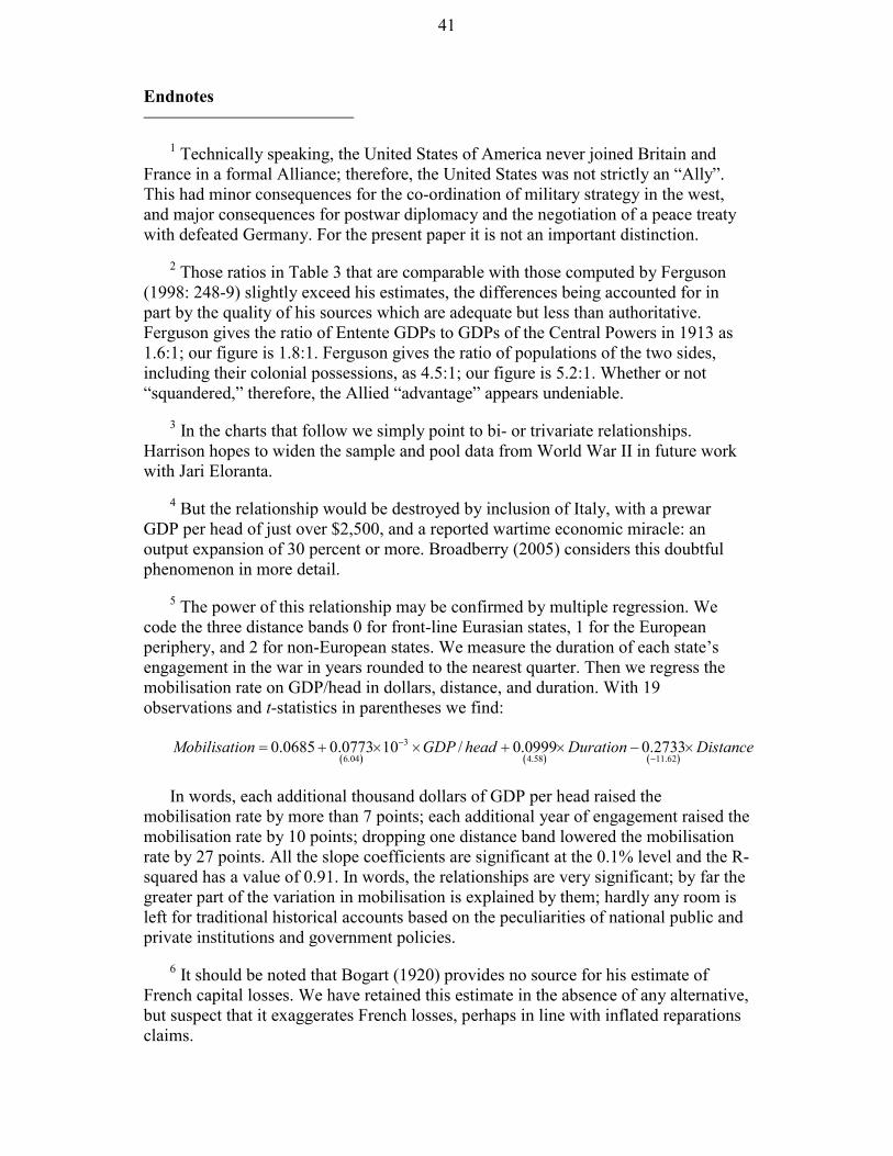
41

Endnotes

1 Technically speaking, the United States of America never joined Britain andFrance in a formal Alliance; therefore, the United States was not strictly an “Ally”.This had minor consequences for the co-ordination of military strategy in the west,and major consequences for postwar diplomacy and the negotiation of a peace treatywith defeated Germany. For the present paper it is not an important distinction.

2 Those ratios in Table 3 that are comparable with those computed by Ferguson(1998: 248-9) slightly exceed his estimates, the differences being accounted for inpart by the quality of his sources which are adequate but less than authoritative.Ferguson gives the ratio of Entente GDPs to GDPs of the Central Powers in 1913 as1.6:1; our figure is 1.8:1. Ferguson gives the ratio of populations of the two sides,including their colonial possessions, as 4.5:1; our figure is 5.2:1. Whether or not“squandered,” therefore, the Allied “advantage” appears undeniable.

3 In the charts that follow we simply point to bi- or trivariate relationships.Harrison hopes to widen the sample and pool data from World War II in future workwith Jari Eloranta.

4 But the relationship would be destroyed by inclusion of Italy, with a prewarGDP per head of just over $2,500, and a reported wartime economic miracle: anoutput expansion of 30 percent or more. Broadberry (2005) considers this doubtfulphenomenon in more detail.

5 The power of this relationship may be confirmed by multiple regression. Wecode the three distance bands 0 for front-line Eurasian states, 1 for the Europeanperiphery, and 2 for non-European states. We measure the duration of each state’sengagement in the war in years rounded to the nearest quarter. Then we regress themobilisation rate on GDP/head in dollars, distance, and duration. With 19observations and t-statistics in parentheses we find:

� � � � � �

3

6.04 4.58 11.620.0685 0.0773 10 / 0.0999 0.2733Mobilisation GDP head Duration Distance�

�

� � � � � � � �

In words, each additional thousand dollars of GDP per head raised themobilisation rate by more than 7 points; each additional year of engagement raised themobilisation rate by 10 points; dropping one distance band lowered the mobilisationrate by 27 points. All the slope coefficients are significant at the 0.1% level and the R-squared has a value of 0.91. In words, the relationships are very significant; by far thegreater part of the variation in mobilisation is explained by them; hardly any room isleft for traditional historical accounts based on the peculiarities of national public andprivate institutions and government policies.

6 It should be noted that Bogart (1920) provides no source for his estimate ofFrench capital losses. We have retained this estimate in the absence of any alternative,but suspect that it exaggerates French losses, perhaps in line with inflated reparationsclaims.

42

7 The relationship is as follows, with t-statistics in parentheses and an R-squaredof 0.59:

(6.93) (14.63)11.04 7.68 1918GDPGrowth GDP� � �