the effect of industrialization on children’s education
TRANSCRIPT

Recommended Citation
Le Brun, A., Helper, S., & Levine. D.I. (2011). The Effect of Industrialization on Children’s
Education. The Experience of Mexico. Review of Economics and Institutions, 2(2), Article 1. doi: 10.5202/rei.v2i2.31. Retrieved from http://www.rei.unipg.it/rei/article/view/31
Copyright © 2011 University of Perugia Electronic Press. All rights reserved
Review of ECONOMICS
and
INSTITUTIONS
Review of Economics and Institutions
www.rei.unipg.it
ISSN 2038-1379 DOI 10.5202/rei.v2i2.31
Vol. 2 – No. 2, Spring 2011 – Article 1
The Effect of Industrialization on Children’s
Education. The Experience of Mexico
Anne Le Brun Susan R. Helper David I. Levine Wellesley College Weatherhead School of Management
Case Western Reserve University University of California,
Berkeley
Abstract: We use census data to examine the impact of industrialization on children’s education in Mexico. We find no evidence of reverse causality in this case. We find small positive effects of industrialization on primary education, effects which are larger for domestic manufacturing than for export-intensive assembly (maquiladoras). In contrast, teen-aged girls in Mexican counties (municipios) with more growth in maquiladora employment 1990-2000 have significantly less educational attainment than do girls in low-growth counties. These results shed light on literatures analyzing the impacts of industrialization, foreign investment, and intra-household bargaining power. JEL classification: I25, L60, O14 Keywords: industrialization, Mexico, maquiladoras
Address: Department of Economics - Wellesley College - 106 Central Street · Wellesley, MA 02481 (Phone 781-283-2988, Email:· [email protected]).

REVIEW OF ECONOMICS AND INSTITUTIONS, Vol. 2, Issue 2 - Spring 2011, Article 1
1 Introduction
During the early 1990s Mexico was a poster child for the “Washing-ton Consensus” of export-led manufacturing growth (Naim, 2000; Hanson,2004). Mexico both increased its manufacturing employment by more thanhalf and shifted from an emphasis on import substitution to export-orientedpolicies. The lion’s share of the increase in manufacturing employmentwas due to export processing plants known as maquiladoras (or maquilas),whose employment more than tripled. Maquilas became the nation’s mostimportant source of export revenue, surpassing even oil.1
The “Peso crisis” in the middle of the decade made clear that export-oriented industrialization was not sufficient to create economic develop-ment. What remains unclear, though, is whether Mexico’s industrializationstrategy was beneficial or harmful to other dimensions of development suchas education.
This question is important because the dimensions of development suchas economic growth, health, and education do not always change in unison(Easterly, 1999). In fact, in some important early cases, industrializationharmed children’s health (Nicholas and Steckel, 1991 and Floud and Harris,1996).
Turning to education, the relationship between manufacturing growthand education is ambiguous. Industrialization may increase education byincreasing parents’ incomes, public sector revenues, returns to skill, and (bypromoting urbanization) children’s access to schools. At the same time,growth in manufacturing jobs can reduce education by increasing the op-portunity costs of keeping children in school, reducing returns to skill (ifmanufacturing jobs are very low skilled), and inducing migration and othersocial disruption that can hinder school attendance.
Importantly for our purposes, some areas of Mexico received far morefactories than others. Also, public school funding was determined by pop-ulation, not local income, thus there is no relationship between the degreeof industrialization of an area and the supply of education there. Our dataalso distinguish manufacturing for the domestic market, and export pro-cessing in maquiladoras. Thus we also examine the differential effects ofglobally-oriented industrialization.
We use household- and municipio-level data from the 1990 and 2000 Cen-suses.2 We construct our sample to focus attention on those municipios atrisk for industrialization. Thus we exclude Mexico City, which was losingmanufacturing jobs. We also exclude very poor rural areas that were af-fected by a large welfare program (Progresa/Oportunidades) that had anindependent effect on children’s enrollment in school. Our main findings
1 Between 1992 and 1999, manufacturing employment increased by 53%, and itsmaquiladora employment jumped by 259%.
2 Municipios resemble U.S. counties.
Copyright c© 2011 University of Perugia Electronic Press. All rights reserved 2

Le Brun, Helper, Levine: The Effect of Industrialization on Children’s Education
are: there is no evidence of reverse causality in plant location. Municip-ios with higher education in 1990 are not more likely to see an increase inmaquila or domestic manufacturing employment than those with lower ed-ucation. These results provide evidence against the hypothesis of endoge-nous factory location. Our specification controls for time-invariant munici-pio characteristics that affect children’s outcomes, though we are still inca-pable of perfectly controlling for the possibility of time-varying municipiocharacteristics. To avoid problems of non-random migration, we focus ouranalysis on non-migrant families, though our results change little when weinclude migrants.
Industrialization, particularly when domestically focused, is correlatedwith higher primary education. In our sample, the percent of the work-force employed in maquilas increased from 2.3% to 4.5% between 1990 and2000. This industrialization is correlated with an increase in educational at-tainment for children aged between 7 and 12 of almost one week (.022 ×.833×52). Had this same increased employment occurred in domestic man-ufacturing, the impact on primary education would have been more thantwice as great. However, growth in maquila employment is significantlycorrelated with lower education a in particular, a doubling in maquiladoraemployment would lower education attainment by one week for teenagergirls.
These effects are small, perhaps because manufacturing work is neitherhigh-skilled nor well-paid relative to other occupations. Increases in man-ufacturing or maquila employment in a municipio do not have a statisti-cally significant impact on household income in that municipio (though thesign is positive), or on skill premia (where the sign is negative). At thesame time, maquilas dramatically increased the demand for women’s labor.When mothers became employed in manufacturing, daughters dropped outof school, presumably to replace mother’s labor in the household. This ef-fect is absent when fathers became employed in manufacturing.
These results shed light on literatures relating to the social effects of in-dustrialization, foreign investment, and intra-household bargaining power.These results suggest that industrialization, if it is focused on low-skill ass-embly-intensive manufacturing, does not increase returns to education. Incontrast to previous literature, we find that providing income to womenmay reduce investments in children, if obtaining the income requires womento work outside the home and does not provide substitutes for women inhousehold labor.
The rest of the paper is structured as follows. We first describe theprocess of maquila-led industrialization that Mexico underwent during the1990s. We then turn to a literature review and theoretical description of howmanufacturing, and maquila manufacturing in particular, may affect chil-dren’s education, by affecting income, urbanization, and intra-householdbargaining. In a third section, we present our empirical methods. We then
http://www.rei.unipg.it/rei/article/view/31 3

REVIEW OF ECONOMICS AND INSTITUTIONS, Vol. 2, Issue 2 - Spring 2011, Article 1
describe our data, and our results.
2 Industrialization and Maquiladoras in Mexico
In this paper, we study the impact of manufacturing-based industrializa-tion on children’s outcomes. We distinguish two types of industrialization:manufacturing for the domestic (Mexican) market and export processing(maquiladoras). We analyze the case of Mexico in the 1990s because thiswas a period of rapid maquiladora growth in the country.3
Until the 1980s, Mexico pursued a relatively closed-border policy of im-port substitution industrialization (ISI). The major exception to this policywas the maquiladora program, a type of Export Processing Zone (EPZ). Thisprogram was started in Mexico in the second half of the 1960s, partly to ab-sorb the Mexican labor force displaced by the United States’ terminationof the Bracero program (a temporary agricultural worker program in theUnited States). Under the maquiladora program, Mexico allowed tax- andtariff-free imports of intermediate goods into plants along the northern bor-der, for assembly and immediate re-export.4 Until 1972 maquilas were bylaw confined to the northern border (Hanson, 2005).
Upon taking office in 1982, President Miguel de la Madrid began a pro-cess of trade and investment liberalization. This paved the way for the even-tual signing of the North American Free Trade Agreement in 1994. The mainimpact of NAFTA was to commit Mexico firmly to a neoliberal regime, rais-ing investor confidence (Hanson, 2004). This market opening led to dra-matic growth of manufacturing in Mexico. Worth only 12 percent of exportsin 1980, manufactured goods accounted for about 43 percent of Mexico’s ex-ports in 1990, and fully 83 percent of its exports by the year 2000 – a growthfrom $95.4 billion real US dollars in 1990 to $138.9 billion in 2000 (WorldDevelopment Indicators, 2000).5
3 This is certainly not the only major change in Mexico’s landscape during the 1990s.Indeed, the country was rocked by the Peso crisis of 1994 too. As a result of this crisis,wages fell significantly between 1990 and 2000 (despite increases in education). Whendeflated by Mexico’s CPI, the average hourly wage in 1990 dollars declined for males from$1.33 to $1.11 and for females from $1.24 to $1.13 (Hanson, 2004).
4 When the North American Free Trade Agreement was implemented in 1994, the tar-iff advantages of maquilas were reduced, although significant tariff savings remained inplace through the end of the period we study (2000). In addition, firms that registeredas maquiladoras in Mexico gained access to a more streamlined paperwork process thanother firms in Mexico, with the government agency SECOFI taking on the responsibilityof registering the firm with many different agencies, for example. Maquiladoras also re-tained important tax advantages. On the other hand, maquiladoras face the obligation tomaintain their inventory in-bond. The combination of these effects means that it is benefi-cial for firms to register as maquiladoras only if they plan to directly export most of theirproduction (INEGI, 2004; Dussel Peters, 2005; Carrillo, personal communication, 2006).
5 Another consequence of the change in trade policy embraced by the de la Madridadministration was the erosion of Mexico City’s privileged position. Under ISI, both the
Copyright c© 2011 University of Perugia Electronic Press. All rights reserved 4

Le Brun, Helper, Levine: The Effect of Industrialization on Children’s Education
The maquila sector proved one of the main drivers of manufacturinggrowth during the 1990s. According to Ibarraran (2003), manufacturing em-ployment grew by 53 percent between 1992 and 1999. In the same time pe-riod, maquila employment shot up by 259 percent.6 In 1992, 67 percent ofmanufacturing employment was in domestic firms, 21 percent was in tra-ditional foreign firms and only 12 percent was in maquiladoras. By 1999,the domestic share had shrunk to 58 percent, the traditional foreign to 14percent, while the share of maquiladora employment had soared to 29 per-cent. In both years, about 80% of the maquiladoras were foreign owned(Ibarraran, 2004, chapter 2 and Table 2A.2).
In our analysis, we distinguish “maquilas” from “domestic manufactur-ing” (both Mexican- and foreign-owned), following Ibarraran (2004). Do-mestic manufacturing is production for the domestic Mexican market. Thesefacilities, many of which date to the ISI period, have relatively high localcontent, so either they or their suppliers perform most of the steps requiredto make the final product within Mexico. For example, domestic apparelmanufacturing included design (selecting fabrics and other inputs, creatingpatterns, and cutting fabric), assembly (sewing pieces together to make agarment), and distribution (Hanson, 1995). Domestic automotive produc-tion involved making components (such as engines, gauges, and wiring),assembling them into finished vehicles, and then distributing them.
In contrast, maquiladoras specialized in just one stage of production, as-sembly. Inputs were imported (even as late as 2000, only 2% of the valueof materials came from Mexico; see Carrillo and Gomis, 2003), assembledin maquilas, and then exported. Thus, apparel maquilas simply sewed to-gether pieces of fabric cut in the US. Automotive parts maquilas assembledproducts such as wiring harnesses, using wire, metal terminals, and plasticconnectors imported from Japan or the US, and then exported the harnessesto the US for final assembly into vehicles (Helper, 1995).
3 Literature Review
Mexico’s episode of rapid maquiladora-centered industrialization in the1990s provides us with a setting in which to assess the short term effectsof manufacturing on children’s education. We first discuss in this section
supply of inputs and the main destination markets for products were within the country(aside from the EPZ project concentrated at the border). With one-quarter of the country’spopulation located in and around Mexico City, this was a good place in which to concen-trate production. As Mexico has shifted its focus to international markets, there was asignificant increase in the benefits of being close to the US, which is both a major source ofinputs, and a vast potential market for outputs (Hanson, 1995).
6 Other sources of data reflect the same trend: the number of 18-65 year old employed inmanufacturing grew by 45% between 1990 and 2000, according to census data. Confiden-tial data obtained by Pablo Ibarraran (2004) put the growth in maquiladora employmentduring the same period at 188%.
http://www.rei.unipg.it/rei/article/view/31 5

REVIEW OF ECONOMICS AND INSTITUTIONS, Vol. 2, Issue 2 - Spring 2011, Article 1
research on the impact of industrialization on development in general. Wethen discuss several channels by which non-maquila manufacturing growthmay affect children’s education, both positively and negatively. Finally, werepeat the exercise for maquila-based growth in manufacturing employ-ment.
The cross-sectional literature has established strong positive correlationsbetween measures of income and measures of well-being. Easterly (1999)summarizes this literature, noting that cross-sectional studies ignore thepossibility of omitted differences across nations, and should therefore not betaken as evidence that growth increases well-being. Easterly also analyzesthe within-country evolution of quality of life across time as a function ofincome growth. His study analyzes income growth, rather than industrial-ization specifically, but since industrialization and GDP growth are highlycorrelated, his conclusions apply to our question as well. Using fixed ef-fects, first differencing or instrumental variables, Easterly finds the relation-ship between growth and quality of life is weaker than in the cross section.Fixed effects and first differences may exacerbate measurement error, buthis findings raise a red flag about the validity of inferring causality fromcross-sectional relationships.
Longitudinal case studies suggest industrialization need not improvewell-being. A variety of evidence supports the contention that living stan-dards fell during the British Industrial Revolution, especially in the 1830sand early 1840s (Nicholas and Steckel, 1991; Floud and Harris, 1996). Re-garding education specifically, the evidence is mixed. For example, Goldinand Katz (1999) find that high school attendance in US was negatively corre-lated with the share of manufacturing employment in the state.7 In contrast,Federman and Levine (2004) find that industrialization has had a positiveimpact on education at all levels in Indonesia.
The inconclusive findings on effects of industrialization on children’s ed-ucation suggest that there is room for further research in this area. Belowwe identify four channels through which a rising share of manufacturingemployment could affect the demand for children’s education: income, ur-banization, family disruption, and education premia. We first discuss thepotential relationship between domestic manufacturing and these channels,and then turn to the link between these channels and maquiladoras.
More manufacturing also leads to increased governmental income, whichcan increase the supply of education (for example, more classrooms andteachers). This effect is muted in Mexico, which had very centralized edu-cation financing during the period under consideration. Changes in man-ufacturing employment in a municipio had little effect on the number ofteachers/student in that municipio, because tax revenues were distributedlargely according to population (see table 5, column 19 below, and also
7 Goldin and Katz (1997) show that average educational attainment in the US in 1890was 8 years – greater than the average for Mexico in 2000.
Copyright c© 2011 University of Perugia Electronic Press. All rights reserved 6
Le Brun, Helper, Levine: The Effect of Industrialization on Children’s Education
Helper et. al., 2006).
3.1 Domestic ManufacturingIncome. Manufacturing is more productive than activities it replaces,
and/or is an additional source of aggregate demand. Hence it raises incomefor families if workers have the bargaining power to share in productivitygains. Increased parental income raises demand for education if educationis a normal consumption good, or if education is constrained by liquidity.However, if manufacturing raises wages and generates employment oppor-tunities, it can raise the opportunity cost of staying in school. Indeed, incontrast to agriculture, which has pronounced peaks of labor demand thatthe school calendar is organized to accommodate, it may be harder to mixmanufacturing work and schooling.
Family disruption. Manufacturing may provide attractive employmentand income prospects which disrupt traditional family structures. By en-couraging families to move to cities away from extended family supportstructures, and by encouraging women to work for pay rather than to en-gage in household production, industrialization may undermine traditionalhousehold mechanisms that support child rearing. If these traditional sup-port structures for children are not replaced (e.g., if fathers do not stayhome), then increased labor force participation of mothers may lead to lesseducation for children, as there may be no one to ensure that children attendschool, or to see that children do their homework. These negative effectsmay be particularly pronounced for older daughters, who may be expectedto stay home and do chores, especially if there are not other adult womenaround to pick up the slack (Chant, 1994).
Education premia. The only kind of skill we (along with most economists)can measure is that conferred by formal education. Predictions here are the-oretically ambiguous. Manufacturing intuitively has higher returns to booklearning than does peasant agriculture. But there is heterogeneity withinmanufacturing, and many jobs are not designed to have a payoff to highschool (Tendler, 2002). So manufacturing may increase the returns to basicliteracy, but not to high school. If education premia rise with manufactur-ing, this provides an incentive to stay in school. Conversely, lower edu-cation premia (especially for high school) increase the opportunity cost ofpostponing entry into work.
Urbanization. Manufacturing often leads to more urbanization, becauseof agglomeration economies across businesses, and because achieving min-imum efficient scale in one business requires a moderately large work force.Urbanization can benefit children by bringing them closer to schools andmaking schools more accessible. One the other hand, the speed of urban-ization may also be important: fast population growth that outstrips con-struction of infrastructure, can lead to overcrowding of schools and poor
http://www.rei.unipg.it/rei/article/view/31 7

REVIEW OF ECONOMICS AND INSTITUTIONS, Vol. 2, Issue 2 - Spring 2011, Article 1
quality of teachers, as well as to unhygienic conditions not conducive tolearning.
3.2 MaquiladorasThe literature on Export Processing Zones’ (EPZ’s) effects on children’s
outcomes is scant. We can however explore what the conclusions of generalpapers on EPZ’s would imply for children’s outcomes. Below, we look athow each of the channels above might be different in the case of maquilado-ras.
Income. Much literature finds that foreign employers pay higher wages.Consistent with this literature, Hanson (2007) finds that exposure to glob-alization (as measured by the share of foreign direct investment, imports,and maquiladoras in states’ GDP) increased income levels in Mexico dur-ing the 1990s. However, as Hanson points out, maquiladoras are only onecomponent of this measure, and the different components may not all havethe same effect on wages. It is also possible that low-globalization statesfared poorly because of globalization in other states; for example, states thatprovided food or manufactured goods to other Mexican states would findtheir incomes reduced when other states began to import these goods fromabroad.
Looking directly at the impact of maquiladoras, Ibarraran (2004) findsthat these plants pay less than other manufacturing employers (see below).An additional piece of evidence is that turnover at maquilas in the 1990s wasextraordinarily high. A survey of employers conducted by Carillo (1993,p. 98) in 1993 in Ciudad Juarez, Tijuana and Monterey found the averageturnover rate was over 30% per month; in late 2000, it was still 10-12% permonth (Hualde, 2001b). Clearly, employers were not attempting to pay effi-ciency wages (see also Helper, 1995).
Family disruption. In addition to affecting levels of income, maquilaemployment may affect who receives the income. A key characteristic ofmaquiladoras is their high share of female employment. There is a greatdeal of evidence that maquila owners had a direct preference for hiringwomen (Tiano, 1993; Helper, 1995). The preference for women existed “be-cause they are more docile”, one manager said (Helper, 1995). Early inour period, maquila employment was overwhelmingly female. But later,as the pool of “maquila-ready” women was exhausted, the percentages fellthroughout the decade. Still, in 1999, while non-maquila manufacturingfirms’ employees were 29 percent female, 49 percent of the maquila laborforce was female (Ibararran, 2003, 2004).8 In the 1980s, managers’ ideal em-
8 Note that according to Ibarraran, while maquiladoras paid 14% less on average thandomestic firms for unskilled labor in 1992, by 1999 the gap had largely closed. During the1990s, turnover in maquilas was quite high in most cities (averaging over 100% per year).Helper (1995) argues that this high turnover was due in large part to the lack of senioritywage incentives. That lack, in turn, was maintained by an employer cartel that kept wages
Copyright c© 2011 University of Perugia Electronic Press. All rights reserved 8
Le Brun, Helper, Levine: The Effect of Industrialization on Children’s Education
ployee was a young, single woman, because they felt that she would not bedistracted by family responsibilities. But by the early 1990s, their preferencehad shifted toward married women, because they showed more stability(Tiano, 1993).
A number of papers have argued against a “unitary” model of familydecision-making in which families pool income from all sources, and ar-gued instead for a “bargaining” model, in which who gets the income affectsfamily decisions. That is, family members are more able to exert their prefer-ence if they bring more income to the table. For example, some papers havefound that increasing the amount of income in women’s hands increases in-vestment in children. For example, Duflo found that increased pension in-come given to grandmothers increased the heights of granddaughters (butnot of grandsons) that lived with them, while pensions given to grandfa-thers had no effect on their grandchildren’s height. Most empirical papersreject the unitary model, but evidence on the impact of women’s bargainingpower on educational investments is mixed (see Xu, 2007 for a review).
These studies do not look at the impact of increased income from labor;instead they look at pre-marital assets, the sex ratio in the marriage market,etc. The reason is that women’s labor hours are usually strongly affected byintrafamily bargaining, so labor income is therefore endogenous. However,income that women receive for working outside the home may have dif-ferent impacts on investment in children than does nonlabor income. Suchemployment by women may well have mixed effects on children’s educa-tion. On the one hand, as discussed above, many women have a strongerpreference for investing in children than their husbands do, and providingmore income increases their bargaining power.
On the other hand, maquila employment may reduce children’s educa-tional attainment for several reasons. First, maquila employment separateswomen from their children, compared not only to women who are full-timehomemakers but also compared to more traditional forms of women’s em-ployment such as running a market stall or performing agricultural work,where children are often present alongside their mothers. Second, maquilaemployment may also raise the opportunity cost of keeping girls in school,if they either are eligible for maquila jobs themselves,9 or are called upon totake over some of the working mother’s chores at home. In Mexico duringthis time period, men rarely men stepped in to perform these chores, evenwhen unemployed (Chant, 1994).
Working conditions at some maquiladoras may also pose health hazardsor be more stressful than other forms of employment. Several studies in the
fixed at the minimum level allowed by law.9 There seem to be fewer employment opportunities for children under 15 years old
in maquiladoras than in other kinds of manufacturing. There is evidence that multina-tionals do not want the bad publicity that might come from hiring children, and that theirproduction processes are less conducive to child labor (Barajas et. al., 2004).
http://www.rei.unipg.it/rei/article/view/31 9

REVIEW OF ECONOMICS AND INSTITUTIONS, Vol. 2, Issue 2 - Spring 2011, Article 1
public health literature provide evidence that at least some maquilas cre-ate health hazards for employees (which could translate into health hazardsfor the children of women who work while pregnant). For example, Eske-nazi et. al. (1993) compared women in Tijuana who worked in services towomen who worked in maquilas making garments and electronic products.They found that the maquila workers’ babies weighed significantly less atbirth. The garment workers’ babies weighed even less than the electronicsworkers’, suggesting that the demands of the job may be a more importantcause of the problem than was occupational exposure to pollutants (as elec-tronics workers were probably exposed to more harmful emissions). Simi-larly, Denman (cited in Cravey, 1998) found that babies born to mothers whoworked in maquilas had lower birth weights, due to chemical exposure andphysical demands on the job than did mothers who worked in service in-dustry. These papers are suggestive, but their evidence is not conclusive, asthey may suffer from sample selection biases if maquilas hire less healthyemployees than do service employers.
Education premia. Industrialization driven by trade opening, as in Mex-ico, has ambiguous effects on the returns to education. The standard trademodel suggests Mexico will specialize in low-skill manufacturing as it in-tegrates with the higher-skilled U.S. market. This specialization can reducethe returns to education. Alternative models (e.g., Feenstra and Hanson,1997) can lead to rising demand for skills, as Mexico shifts to jobs whichfor Mexico are medium-skilled, even if for the US they fit into the cate-gory of relatively low-skilled jobs. Feenstra and Hanson (1997) find thatin states with more maquiladoras, the wage differential between produc-tion and non-production workers grew over the 1980s.10 But studies us-ing data for the 1990s do not connect maquiladoras to the rising skill pre-mium. These scholars characterize maquiladoras as low-skill-intensive sec-tors, whose boom in the 1990s led to fast employment growth, but did notcontribute to the rise in the skill premium.11
Some have argued that maquilas began in the late 1990s to include moreskill-intensive activities (beyond assembly) (Carrillo et. al., 1998; Carrillo
10 Hanson (2004) provides two additional possible reasons for the rise in skill premium.First, low-skill sectors saw the steepest fall in protection in the early wave of liberalization.By the Stolper Samuelson theorem, this would lead to a widening of the wage gap betweenskilled and unskilled workers. Second, capital and skilled labor are complements, so thatthe inflow of capital into the export processing sector generated by trade liberalization ledto a rise in demand for skilled labor, driving up the skill premium.
11 Ibarraran (2004) uses data from the ENESTYC (the National Survey of Employ-ment, Salaries, Technology and Training in the Manufacturing Industries), and shows thatmaquiladora workers in 1992 had lower average skill, lower median wages (for every skilllevel), and lower capital-to-labor ratios than all other manufacturing. By 1999, maquilado-ras’ median wages by skill level had closed the gap with domestic non-maquiladora man-ufacturing, but the skills distribution of maquiladora workers remained lower than aver-age for manufacturing and the capital-intensity of production remained much lower in themaquiladora sector.
Copyright c© 2011 University of Perugia Electronic Press. All rights reserved 10

Le Brun, Helper, Levine: The Effect of Industrialization on Children’s Education
and Hualde, 1996). However, the percentage of maquiladora employeeswho were engineers or technicians as opposed to operators did not changeover our period (INEGI, 2004; Hualde, 2001b). As Verhoogen (2008) notes,“Although there may have been a shift toward more skill-intensive activitieswithin the maquiladora sector, it appears that the first-order consequence ofthe expansion of the sector was an increase in the demand for less-skilled la-bor.” Maquiladoras require a minimum level of education, but this is eithera 6th grade or less commonly an 8th grade diploma (Tiano, 1993; Helper,1995). Such a policy would raise the demand for early education, but notfor high school.
Urbanization. As discussed above, Mexico reversed course in the 1980s,moving from import substitution to neo-liberal growth policies, and thispolicy shift led to a dramatic increase in the attractiveness of investment inmaquiladoras. Thus, to the extent that fast urbanization has bad effects onchildren, these effects should be particularly evident in areas with a highpercentage of maquila employment, which saw a faster urbanization rate.
The bottom line is that the effect of maquiladora growth on demand foreducation is theoretically ambiguous.
4 Methods
In this section, we introduce the basic empirical model we will be esti-mating. We then review concerns about this model and our approaches todealing with them.
4.1 Basic SpecificationIt is impossible to predict a priori the direction of industrialization’s ef-
fects on children. This ambiguity motivates our empirical analysis. We usethe following basic specification to assess the sign of manufacturing andmaquiladoras’ impacts on children:
School − yrsi,m,t = α+ β %MFGm,t + φ %MAQm,t + γ Xi,m,t +
δm FEm + θ year2000 +
λ %MFGm,1990 × year2000 + π %MAQm,1990 × year2000 +
ρ School − yrsm,1990 × year2000 + εi,m,t (1)
where i represents a child, m is his/her municipio of residence, and t iseither 1990 or 2000. The dependent variable is the number of school yearsthe child has completed. The variables %MFGm,t and %Maqm,t are the mainvariables of interest: they are the percentage of people aged between 18and 65 in the municipio who are employed in non-maquila manufacturingand maquiladoras, respectively, at time t. The X’s are household and childcharacteristics, FEm are municipio fixed effects, and year2000 is a dummyequal to 1 in the year 2000. We also attempt to control for effects of 1990
http://www.rei.unipg.it/rei/article/view/31 11

REVIEW OF ECONOMICS AND INSTITUTIONS, Vol. 2, Issue 2 - Spring 2011, Article 1
characteristics on outcomes in the year 2000, by including in the year 2000the lagged values of %MFGm, %MAQm and of the dependent variable’saverage value for the child’s age group.
This specification is similar to an equation in changes, but allows us tocombine household-level observations from 1990 with those from 2000.
4.2 Potential Difficulties and SolutionsThe specification above faces a number of challenges. We list here the
main issues, and our approaches to them.
Table 1 - Testing for Endogenous Manufacturing/Maquiladora Location
Table 1: Testing for Endogenous Manufacturing/Maquiladora Location
Dependent variable Δ# adults employed in maquila OR non-maquila manufacturing m/population m,1990
Δ# adults employed in maquilas m/population m,1990
(1) (2) (3) (4)
Mean educationm,1990 0.002 (0.011)
-0.005 (0.010)
0.009 (0.012)
0.015 (0.012)
(Mean education)2m,1990
-0.001 (0.001)
-0.000 (0.001)
-0.001 (0.001)
-0.001 (0.001)
Fraction of 18-65 year olds employed in non-maquila manufacturing m,1990
0.413*** (0.048)
0.403 (0.046)***
0.117 (0.053)**
0.065 (0.051)
Fraction of 18-65 year olds employed in maquilasm,1990
0.032 (0.024)
0.025 (0.024)
0.525 (0.027)***
0.520 (0.027)***
Fraction urban in 1990 0.017 (0.013)
0.005 (0.013)
0.014 (0.014)
0.010 (0.014)
D=1 if municipio is on North border
-0.006 (0.005)
-0.009 (0.005)*
0.030 (0.006)***
0.034 (0.006)***
Fraction of population w/toilet in 1990
-0.060 (0.017)***
---- 0.043 (0.019)**
----
Fraction of population w/sewage in 1990
0.003 (0.011)
---- -0.040 (0.013)***
----
Fraction of population w/electricity in 1990
-0.010 (0.028)
---- 0.004 (0.031)
----
Constant 0.056 (0.034)
0.037 (0.031)
-0.051 (0.038)
-0.048 (0.034)
Observations 405 405 405 405
R-squared 0.33 0.30 0.71 0.70
Notes: OLS, municipio-level regressions. Robust errors clustered at year×municipio, shown in parentheses. Significant at *** 1%, ** 5% and * 10% levels. All regressions are
weighted using weights provided by IPUMS. Municipios with more than 10% of HH receiving Progresa/Procampo, and Municipios in Mexico City are excluded.
Notes: OLS, municipio-level regressions. Robust standard errors clustered at year×municipio, shown in paren-theses. Significant at *** 1%, ** 5% and * 10% levels. All regressions are weighted using weights provided byIPUMS. Municipios with more than 10% of HH receiving Progresa/Procampo, and Municipios in Mexico City areexcluded.
4.2.1 Reverse Causality
The first issue is the possibility of reverse causality, or endogenous fac-tory location. It is possible that manufacturers seek out the most educatedworkers and therefore locate in municipios with high pre-existing educa-tional attainment. If this were true, we would expect to see municipioswith high educational levels in 1990 having more manufacturing employ-ment growth from 1990 through 2000 than those municipios with poor 1990education statistics. To assess whether this is the case, we regress the mu-nicipio’s 1990-2000 growth in manufacturing employment (maquila or oth-
Copyright c© 2011 University of Perugia Electronic Press. All rights reserved 12
Le Brun, Helper, Levine: The Effect of Industrialization on Children’s Education
erwise) on baseline (1990) indicators of (i) the municipio’s average adulteducation and (ii) education squared. Positive and significant coefficientson these variables would suggest that there is indeed endogenous factorylocation. In the regression, we control for the percentage of the municipiosthat was urbanized as of 1990. We also include as controls baseline indus-trialization of the municipio and baseline infrastructure measures. We thenrepeat the analysis using as the dependent variable the municipio’s 1990-2000 growth in maquiladora employment. As Table 1 illustrates, we find nosignificant relationship between baseline education indicators and industri-alization (whether domestic or maquila). Thus, there is no strong evidenceof endogenous factory location. These results are robust to a variety of spec-ifications.
4.2.2 Endogenous Migration
Another challenge is the possibility of endogenous migration within Mex-ico. People with more skills and ambition may migrate from the countrysideto cities with high industrial growth, sensing higher opportunities there;these people may also be more likely to invest in their children’s education.This selective migration can generate a positive correlation between manu-facturing and children’s outcomes due entirely to selection into migrationof the most able, and not due to a causal relationship between manufactur-ing and children’s outcomes. On the other hand, it is also possible that themost desperate families, those least able to invest in their children, are thosethat migrate into areas of high factory growth. If so, the correlation betweenmigration and children’s outcomes would be a negative one and the truebenefits of manufacturing growth would be greater than estimated.
To deal with this issue, we present all our results excluding familiesnot currently residing in the Mexican state in which the mother was born.This does not change our results substantially; results including immigranthouseholds are available upon request.
4.2.3 Explanatory Variables Influenced by Industrialization
A third issue is the joint determination of some of the right-hand sidevariables. In particular, some explanatory variables may be influenced byindustrialization. For instance, employment of a female household memberin the manufacturing sector affects the care that a child receives, but the em-ployment of a female household member is likely affected by the degree ofindustrialization in the municipio. In our opinion, this need not be a prob-lem. Any right-hand side variable that is endogenous to manufacturing infact represents a “mediating channel” through which manufacturing affectschildren. Methodologically, the concern with this type of variable is thatits correlation with manufacturing will lower the precision of our estimates,but from a practical stand-point, we are interested in this multicollinearitybecause it can help us pinpoint more precisely through what channels man-ufacturing is affecting children.
http://www.rei.unipg.it/rei/article/view/31 13

REVIEW OF ECONOMICS AND INSTITUTIONS, Vol. 2, Issue 2 - Spring 2011, Article 1
We first present a parsimonious version of our basic specification, in-cluding in our regressions only those explanatory variables which are ar-guably exogenous to industrialization: child’s age, percent of children inthe household who are male, and mother’s educational attainment, with theunderstanding that this parsimonious specification may suffer from omittedvariable bias. We then repeat the regressions including a broader set of con-trols, some of which may be endogenous to industrialization.
4.2.4 Omitted Factors
A final and related difficulty with the basic specification presented hereis that there could be omitted factors which determine both factory locationand education in a municipio, even when the broader set of controls are in-cluded. If these factors are time-invariant, the inclusion of the municipiofixed effects in our basic specification deals with the problem. However, ifthere are time-varying municipio characteristics which determine both fac-tory location and educational outcomes for children, our basic specificationabove (and that with more control variables too) will suffer from omittedvariable bias. As no perfect instrument for manufacturing growth exists,the best we can do for now is to identify and control for the factors whichcould be differentially affecting municipios over time.
One example of time-varying municipio characteristics is the Oportu-nidades program. Oportunidades, launched in 1998 by the federal govern-ment (initially called Progresa), provides financial aid to families that keeptheir children in school and take them to clinics for regular health check-ups.At year end 1999, the program was in place for 2000 rural municipios, outof 2443 total municipios in Mexico (Skoufias, 2005). Because the programwas a purely rural one in 2000, there is likely to be a negative correlation inour 2000 data between municipios with high manufacturing employmentand municipios with household that participate in Oportunidades. Usingour basic specification, we could find that the coefficient on manufacturingintensity is negative, but it is possible that this would reflect the positiveimpact of Oportunidades in rural communities, rather than the negativeeffect of manufacturing in urban municipios. To deal with this issue, weremove from our sample all municipios in which more than ten percent ofthe household claim to receive Oportunidades benefits in 2000.
It is difficult to uncover and control for all factors which could be affect-ing both industrialization and children’s outcomes differently in differentmunicipios. However, it should be noted that if our analysis does sufferfrom omitted variable bias, the nature of the bias would have to be rathercomplicated to explain our results, as will become apparent below.
4.3 DataOur main sources of data are the IPUMS (Integrated Public Use Micro-
data Series) 10 percent and 10.6 percent samples of Mexico’s 1990 and 2000censuses, respectively.
Copyright c© 2011 University of Perugia Electronic Press. All rights reserved 14

Le Brun, Helper, Levine: The Effect of Industrialization on Children’s Education
Table 2 - Summary Statistics, Census 1990, 2000
1990 2000
1990 2000
Maquila Non-maquila Maquila Non-maquila
# observations 3039208 2805903 1619540 1419668 1707699 1098204
Fraction of municipio 18-65 year olds employed in non-maquila manufacturing
0.052 0.051 0.053 0.051 0.050 0.055
Fraction of municipio 18-65 year olds employed in maquilas 0.023 0.045 ---- ---- ---- ----
Fraction of municipio 18-65 year old women employed in manufacturingg†
0.028 0.043*** 0.036 0.018*** 0.050 0.028***
Fraction household 18-65 year old women employed in maquila or non-maquila manufacturing
0.043 0.074*** 0.056 0.027*** 0.086 0.047***
Fraction household 18-65 year old men employed in maquila or non-maquila manufacturing
0.206 0.208 0.232 0.176*** 0.229 0.158***
Fraction of kids whose mother works in maquila or non-maquila manufacturing†
0.029 0.068*** 0.037 0.020*** 0.078 0.045***
Fraction of kids whose father works in maquila or non-maquila manufacturing †
0.209 0.216*** 0.235 0.180*** 0.239 0.167***
School years completed:
7-12 year olds 13-15 year olds 16-18 year olds 19-21 year olds 22-25 year olds 26-45 year olds
2.89 6.60 8.02 8.58 8.62 7.09
3.10*** 7.09*** 8.89*** 9.66*** 9.67*** 8.99***
2.94 6.73 8.17 8.78 8.92 7.50
2.84*** 6.46*** 7.86*** 8.34*** 8.24*** 7.61***
3.12 7.16 8.99 9.79 9.82 9.25
3.07*** 6.94*** 8.68*** 9.36*** 9.35*** 8.39***
Mothers’ average education 5.51 7.26*** 5.89 5.08*** 7.56 6.59***
Mothers’ average age 40.3 41.4*** 40.3 40.2*** 41.40 41.40
Average household size 4.80 4.18*** 4.76 4.84*** 4.15 4.23***
Average age of household head 43.6 44.6*** 43.4 43.7*** 44.5 44.9***
Fraction of children w/ father home 0.809 0.812*** 0.821 0.803*** 0.813 0.801***
Fraction of children w/ mother home 0.903 0.932*** 0.908 0.898*** 0.935 0.926***
Average log(earnings of HH head or spouse) 7.98 8.01*** 8.08 7.85*** 8.11 7.77***
Fraction of households with toilets 0.862 0.957*** 0.910 0.807*** 0.972 0.926***
Fraction of households with sewage 0.702 0.817*** 0.761 0.634*** 0.856 0.731***
Fraction of households with electricity 0.938 0.981*** 0.952 0.923*** 0.985 0.973***
Fraction of households that are urban 0.882 0.900*** 0.929 0.828*** 0.932 0.827***
Fraction of household members ≤18 years old 0.382 0.331*** 0.375 0.390*** 0.327 0.339***
Fraction of household members 22-64 years old 0.467 0.518*** 0.474 0.459*** 0.523 0.505***
Fraction of household members ≥65 years old 0.069 0.081*** 0.069 0.070 0.079 0.084***
Fraction of household members who are males 0.467 0.465*** 0.469 0.464*** 0.467 0.462***
Source: IPUMS 10% samples of 1990 and 2000 Mexican Census. Notes: Excludes immigrant households, Mexico City, and households in municipios with >10%
Oportunidades participation. Notes: 1990-2000 or maquila-non maquila difference is significant at ***1%, ** 5% or * 10% level. † Given that our maquila employment data is
derived from a different survey, the only information we have for maquilas is percent of the population in a municipio which is employed in maquiladoras. We can subtract this
number from the percent employed in manufacturing to obtain an estimate of the percent of the municipio’s population employed in non-maquila manufacturing. For all other
manufacturing-related variables, we cannot distinguish between maquiladora and non-maquiladora employment.
Notes: Excludes immigrant households, Mexico City, and households in municipios with ¿10% Oportunidadesparticipation. Notes: 1990-2000 or maquila-non maquila difference is significant at ***1%, ** 5% or * 10% level.†Given that our maquila employment data is derived from a different survey, the only information we have formaquilas is percentage of the population in a municipio which is employed in maquiladoras. We can subtract thisnumber from the percentage employed in manufacturing to obtain an estimate of the percentage of the municipio’spopulation employed in non-maquila manufacturing. For all other manufacturing-related variables, we cannotdistinguish between maquiladora and non-maquiladora employment.Source: IPUMS 10% samples of 1990 and 2000 Mexican Census.
We also have data on maquiladora employment levels by municipio in1990 and 2000 (aggregated from maquiladora surveys conducted by INEGI,and made available to us by Pablo Ibarraran). We use this data to constructthe percentage of 18-65 year old population in the municipio who are em-ployed in maquiladoras. The census identifies people who work in man-ufacturing generally. By subtracting our maquiladora employment figures,we are thus able to come up with an estimate of the percent of 18-65 year oldin the municipio who are employed in non-maquila manufacturing. Thesemeasures of maquiladora and non-maquila manufacturing intensity are ourkey measures of the degree and type of a municipio’s industrialization.
http://www.rei.unipg.it/rei/article/view/31 15
REVIEW OF ECONOMICS AND INSTITUTIONS, Vol. 2, Issue 2 - Spring 2011, Article 1
The outcome that interests us is educational attainment, i.e. school yearscompleted. Summary statistics are presented in Table 2, for residents of481 of Mexico’s 2443 municipios.12 We have deleted from this data all themunicipios that make up Mexico City (because by 1990, Mexico City wasalready undergoing a process of de-industrialization, which is not the phe-nomenon we are interested in studying), and all the municipios in whichmore than ten percent of households participate in Oportunidades or Pro-campo.13 We also exclude from this data immigrant families. Columns 3through 6 contrast the means of variables in municipalities with no maquilaemployment to those in municipalities where maquiladoras have chosen tolocate.
Our measure of income includes income to the household head andspouse, but not to other members of the household. It does not includeincome to children or other adults living in the household. It is unclearwhat happens to income earned by these household members; some stud-ies find that most of teenagers’ earnings is kept by them, while others findthat the money is turned over to the household head (Tiano, 1993). In anycase, our results do not change if income of children and other family mem-bers is included. Our income measure does not capture benefits, whichwere greater for formal sector employment like manufacturing (domesticor maquila) than they were for informal employment. Thus, we may be dis-proportionately underestimating income to manufacturing households.14
We do not include emigrant remittances; this omission would bias our re-sults about manufacturing only if households participating in manufactur-ing were more likely to receive such remittances. There is no evidence thatthis is true; emigrants are not more likely to come from areas near the USborder (Hanson, 2009).
12 In 1990, Mexico had only 2,402 municipios. To match 1990 and 2000 data at the mu-nicipio level, we have merged municipios which were created during the decade back intotheir origin municipio of 1990. Our final data set has 405 municipios. Where did thesemunicipios go? First, we grouped the 600 municipios in the state of Oaxaca (each of whichis tiny) into 20 larger districts, using code from Chris Woodruff (see Helper et al, 2006).Second, we dropped municipios with significant Progresa exposure (as described below),and third, we dropped all “Mexico City” municipios, which we defined as all municipiosin the Distrito Federal plus 18 additional municipios in the Estado de Mexico that borderthe Distrito. We are left with 481 municipios, representing 32% of the observations in theoriginal sample.
13 The census asks respondents in 2000 if they receive Progresa (Oportunidades) orProcampo benefits. Thus, it is unclear, when we delete municipalities with high Opor-tunidades participation, whether we are not sometimes attributing to Oportunidades ben-efits received from Procampo. In any case, the average percent of 18-65 year old populationemployed in manufacturing (maquila or otherwise) is 12.5% in the municipalities we keepin our analysis, versus 6.3% in those we throw out as “significant” Progresa/Procamporecipients.
14 However, including a measure of benefits in household income would not increaseour measure of skill premia in maquiladoras, since those workers are less educated thanthe average worker.
Copyright c© 2011 University of Perugia Electronic Press. All rights reserved 16

Le Brun, Helper, Levine: The Effect of Industrialization on Children’s Education
The summary statistics on municipios with and without maquiladoraspresent a mixed picture. Growth in manufacturing during the 1990s wasclearly focused in the maquiladora sector — its share of employment dou-bled during the 1990s, while the percent of 18-65 year old employed in non-maquila manufacturing remained essentially unchanged. Average schoolyears completed rose more quickly in municipios with no maquiladorasthan in municipios with maquiladoras in 1990, but from a lower base.
Table 3 - Fixed Effects Estimates of Industrialization’s Effect on Educational Attain-ment
Table 3: Fixed Effects Estimates of Industrialization’s Effect on Educational Attainment
Dependent variable Number of school years completedi,m,t
Ages 7-12 13-15 16-18
(1) (2) (3)
Fraction 18-65 year olds employed in non-maquila manufacturing m,t
1.792 (0.396)***
1.319 (0.423)***
-0.15 (0.631)
Fraction 18-65 year olds employed in maquilas m,t 0.833 (0.250)***
0.56 (0.254)**
-0.359 (0.337)
Fraction 18-65 year olds employed in non-maquila manufacturing m,1990 × 2000 Dummy
0.462 (0.200)**
0.643 (0.244)***
0.368 (0.349)
Fraction 18-65 year olds employed in maquilas m,1990× 2000 Dummy
0.509 (0.093)***
0.703 (0.096)***
0.797 (0.136)***
Dummy=1 if male -0.101 (0.004)***
-0.15 (0.009)***
-0.116 (0.019)***
Mother's years of education 0.056 (0.002)***
0.124 (0.003)***
0.228 (0.003)***
Fraction of household kids who are male 0.000 -0.006
-0.019 -0.012
-0.038 (0.015)***
Year 2000 dummy 1.495 (0.118)***
3.109 (0.130)***
2.985 (0.131)***
Avg yrs of schooling of 7-12 yr olds in 1990 * 2000 Dummy -0.491 (0.042)***
---- ----
Avg yrs of schooling of 13-15 yr olds in 1990 * 2000 Dummy ---- -0.446 (0.020)***
----
Avg yrs of schooling of 16-18 yr olds in 1990 * 2000 Dummy ---- ---- -0.325 (0.016)***
Constant 2.087 (0.026)***
5.269 (0.030)***
6.800 (0.040)***
Observations 696057 410131 380617
R-squared 0.61 0.23 0.19
Test of joint significance of first two coefficients 10.23 5.25 0.62
Test of equality of first two coefficients 11.75 3.98 0.14
Notes: all regressions exclude people living in Mexico City or municipios where at least 10% of the population receives Progresa/Procampo, and exclude all members of immigrant
households. Regressions are OLS, and include age dummies, not shown. Errors, clustered at year×municipio, shown in parentheses. Significant at *** 1%, ** 5% and * 10% levels.
All regressions are weighted using weights provided by IPUMS. The test statistics are F statistics.
Notes: all regressions exclude people living in Mexico City or municipios where at least 10% of the populationreceives Progresa/Procampo, and exclude all members of immigrant households. Regressions are OLS, andinclude age dummies, not shown. Standard errors, clustered at year×municipio, shown in parentheses. Signif-icant at *** 1%, ** 5% and * 10% levels. All regressions are weighted using weights provided by IPUMS. The teststatistics are F statistics.
4.4 ResultsWe first present a parsimonious specification of manufacturing’s effects
on children’s education, and then repeat the regressions with more controlvariables.
http://www.rei.unipg.it/rei/article/view/31 17

REVIEW OF ECONOMICS AND INSTITUTIONS, Vol. 2, Issue 2 - Spring 2011, Article 1
4.4.1 Results with Parsimonious Specification
Table 3 presents the results from our basic specification, including mu-nicipio fixed effects and year dummies, and only those right-hand side con-trol variables which are most clearly exogenous or predetermined (namelygender and age dummies, mother’s education, and a control for the shareof household kids who are male). The regressions are broken down by agegroup — we run one regression for 7-12 year old population (i.e., children ofgrade school age), one for children 13-15 years old (who should be in juniorhigh) and one for children 16-18 years old, or of high school age. The tablesuggests that non-maquiladora and maquiladora industrialization are bothassociated with higher educational attainment for seven to 15 year old. Theeffects are not large; a doubling of a municipio’s percent maquila employ-ment, as occurred in the 1990s, would be correlated with about a week moreof education; the effect of non-maquila manufacturing is twice as big as formaquilas.15
The coefficients on both non-maquila manufacturing and maquila em-ployment are negative but insignificant for 16 to 18 year old people. Giventhat school years are cumulative, one might expect that gains in school-ing achieved early in life would translate into higher educational attain-ment throughout life. However, the fact that the coefficient for 16-18 yearold is no longer significant implies that while non-maquila manufacturingand maquiladoras encourage early childhood education, they may discour-age schooling for older children. Maquiladoras require a minimum levelof education, but this is either a 6th grade or less commonly an 8th gradediploma (Tiano, 1993; Helper, 1995). Such a policy would raise the demandfor early education and the opportunity cost of further education in thehigh-industrialization municipios relative to the low-industrialization mu-nicipios.16
As far as the other right hand side variables are concerned, historicalnon-maquila manufacturing and maquiladora employment underscore theeffect of current non-maquila manufacturing and maquiladoras: in mu-
15 We have also averaged the data at the municipality-level and run first-difference re-gressions (including as controls lagged values of %MFGm, %MAQm, and the dependentvariables), and we find qualitatively similar results. We show here the individual-levelregressions because these allow us to include more precise controls and will facilitate thecausal-channel analysis. We cluster all errors with the interaction year × municipio. We havealso run separate regressions for each year of age (rather than grouping children 7-12, forexample) and also run all regressions using the number of school years completed relativeto the average for the child’s age, and results are very similar.
16 Of course it is possible also that manufacturing intensity is strongly correlated withurbanization, and it is the proximity to any kind of employment possibility, not just man-ufacturing jobs, that may take children in high-manufacturing-intensity municipios out ofschool earlier. In results available on request, when we include a dummy=1 if child livesin an urban environment in the regressions, the regression results do not change. Thissuggests that we are not wrongly attributing to industrialization an effect that is actuallyattributable to urbanization.
Copyright c© 2011 University of Perugia Electronic Press. All rights reserved 18

Le Brun, Helper, Levine: The Effect of Industrialization on Children’s Education
nicipios which had high industrialization of either type in 1990, childrenbetween 7 and 15 had higher school years completed in 2000.17 As ex-pected, maternal education is positively correlated with a child’s educa-tional achievement. As in many countries, boys have lower educationalattainment than girls.
In Table 4, we reproduce the same regressions, distinguishing betweengirls (columns 1 through 3) and boys (columns 4 through 6). While bothtypes of industrialization have benefits for primary school for both sexes,girls between 13 and 15 benefit only from domestic manufacturing, whileboys benefit from both types of manufacturing. The detrimental effect ofthe municipio’s maquiladora employment is particularly salient for 16-18year old girls. For them, the coefficient on municipio maquiladora employ-ment is not only negative but also significant; girls between 16 and 18 wouldlose more than a week of educational attainment if the percentage maquilaemployment in their municipio doubled.
Table 4 - Fixed Effects Estimates of Industrialization’s Effect on Educational Attain-ment - Girls vs. Boys
Table 4: Fixed Effects Estimates of Industrialization’s Effect on Educational Attainment – Girls v. Boys
Dependent variable Number of school years completed i,m,t Gender Girls Boys Ages 7-12 13-15 16-18 7-12 13-15 16-18 (1) (2) (3) (4) (5) (6) Fraction 18-65 year olds employed in non-maquila manufacturing m,t
2.012 (0.422)***
1.678 (0.462)***
-0.67 -0.815
1.629 (0.411)***
1.035 (0.575)*
0.527 (0.694)
Fraction 18-65 year olds employed in maquilas m,t
0.662 (0.258)**
0.271 -0.24
-1.095 (0.373)***
1.025 (0.263)***
0.89 (0.365)**
0.517 (0.432)
Fraction 18-65 year olds employed in non-maquila manufacturing m,1990 × 2000 Dummy
0.456 (0.210)**
0.83 (0.257)***
0.823 (0.382)**
0.457 (0.214)**
0.411 (0.316)
-0.08 (0.429)
Fraction 18-65 year olds employed in maquilas m,1990× 2000 Dummy
0.484 (0.104)***
0.559 (0.092)***
0.639 (0.241)***
0.529 (0.100)***
0.841 (0.156)***
0.963 (0.209)***
Dummy=1 if male
Mother's years of education 0.052 (0.002)***
0.119 (0.003)***
0.227 (0.004)***
0.059 (0.002)***
0.127 (0.003)***
0.228 (0.004)***
Fraction of household kids who are male
-0.117 (0.008)***
-0.279 (0.018)***
-0.274 (0.021)***
0.101 (0.009)***
0.253 (0.018)***
0.248 (0.021)***
Year 2000 dummy 1.493 (0.119)***
3.456 (0.128)***
2.879 (0.154)***
1.491 (0.131)***
2.768 (0.171)***
3.062 (0.144)***
Avg yrs of schooling of 7-12 yr olds in 1990 * 2000 Dummy
-0.49 (0.042)***
---- ---- -0.492 (0.045)***
---- ----
Avg yrs of schooling of 13-15 yr olds in 1990 * 2000 Dummy
---- -0.495 (0.020)***
---- ---- -0.401 (0.026)***
----
Avg yrs of schooling of 16-18 yr olds in 1990 * 2000 Dummy
---- ---- -0.300 (0.018)***
---- ---- -0.349 (0.018)***
Constant 2.13 (0.027)***
5.349 (0.033)***
6.876 (0.051)***
1.919 (0.028)***
4.948 (0.038)***
6.468 (0.049)***
Observations 342644 205463 191955 353413 204668 188662
R-squared 0.62 0.24 0.20 0.59 0.23 0.19
Test of joint significance of first two coefficients
12.03 7.58 4.96 9.08 3.49 0.75
Test of equality of first two coefficients
20.09 14.71 0.41 4.22 0.07 0.00
Notes: all regressions exclude people living in Mexico City or municipios where at least 10% of the population receives Progresa/Procampo, and exclude all members of
immigrant households. Regressions are OLS, and include age dummies, not shown. Errors, clustered at year×municipio, shown in parentheses. Significant at *** 1%, ** 5% and *
10% levels. All regressions are weighted using weights provided by IPUMS. The test statistics are F statistics.
Notes: all regressions exclude people living in Mexico City or municipios where at least 10% of the populationreceives Progresa/Procampo, and exclude all members of immigrant households. Regressions are OLS, andinclude age dummies, not shown. Standard errors, clustered at year×municipio, shown in parentheses. Signif-icant at *** 1%, ** 5% and * 10% levels. All regressions are weighted using weights provided by IPUMS. The teststatistics are F statistics.
17 The effect extends to 16 to 18 year old for maquiladoras.
http://www.rei.unipg.it/rei/article/view/31 19

REVIEW OF ECONOMICS AND INSTITUTIONS, Vol. 2, Issue 2 - Spring 2011, Article 1
4.4.2 Results with Control Variables
We are interested in identifying the channels through which industri-alization affects the demand for children’s education. In this section, weinvestigate the impact of the four causal channels discussed in the pre-vious section (income, family disruption, skill premia, and urbanization).The goal is to see if in fact manufacturing employment growth did havethe hypothesized impact of, for example, raising income. Thus, we regressthe 1990-2000 change in each potential mediating variable on the change inmanufacturing employment, controlling for certain baseline characteristics.The results of these regressions are presented in Table 5.
Before discussing these demand-side factors, we first point out that man-ufacturing and maquila growth did not affect the supply of education. Col-umn 19 shows that increases in industrial employment did not affect teacher-student ratios, consistent with the argument that, since Mexico financedschools centrally during this period, industrialization did not affect the sup-ply of schooling.
Surprisingly, there is little evidence for three of the four causal chan-nels on the demand side. An increase in either type of manufacturing em-ployment does not increase income (including proxies for income such asparents’ education, toilets, sewers and electricity; see cols. 9-13), does notincrease urbanization (col. 1), and does not increase skill premia (cols. 20-22).
The one channel that does operate as predicted is household structure.Increased maquila employment in the municipio increases the percentage ofhousehold females employed in manufacturing, and increases the percent-age of children whose mother is employed in manufacturing (given that themother is present in the home). An increase in either type of industrial em-ployment is correlated with an increase in the likelihood that a child’s fatheris employed in manufacturing, given that the father lives at home.18
Having identified at least some of the potential mediating variables thatare affected by industrialization, we now include them in our educationalattainment regressions (Table 6 and Table 7). We find some support for thetheory that more maquilas in a municipio leads to more women in a house-hold being employed in manufacturing, and that this increase causes girls’education to suffer.
18 Note that effect of manufacturing growth on paternal industrial employment issmaller when the manufacturing growth is concentrated in the maquiladora sector.
Copyright c© 2011 University of Perugia Electronic Press. All rights reserved 20

Le Brun, Helper, Levine: The Effect of Industrialization on Children’s Education
Tabl
e5
-Ass
essi
ngC
ausa
lCha
nnel
sof
Indu
stri
aliz
atio
n
Table
5:
Assessin
g C
ausal
Channels
of I
ndustr
iali
zati
on
Δ
%
urb
an
Δ
in
% H
H
fem
ale
s e
mp
loy
’d
in m
fg
Δ i
n a
vg
H
H h
ea
d
ag
e
Δ i
n a
vg
%
HH
m
em
be
rs<
18
y
rs o
ld
Δ i
n a
vg
H
H s
ize
Δ
in
av
g %
H
H ≥
65
ye
ars
old
Δ i
n a
vg
%
HH
22
-64
yrs
old
Δ i
n a
vg
%
HH
ad
ult
s w
ho
a
re
m
ale
Δ i
n a
vg
%
HH
w/
toil
et
Δ i
n a
vg
%
HH
w/
se
wa
ge
Δ i
n a
vg
%
HH
w/
ele
ctr
icy
(1)
(2)
(3)
(4)
(5)
(6)
(7)
(8)
(9)
(10
) (1
1)
Δ i
n %
mfg
-0
.09
6
(0.1
20
) 0
.16
2
(0.1
33
) -1
6.9
34
(7
.83
7)*
-0
.08
3
(0.1
36
) -0
.05
4
(0.8
40
) -0
.01
9
(0.0
35
) -0
.05
1
(0.0
64
) -0
.04
9
(0.1
29
) 0
.08
1
(0.1
55
) 0
.05
6
(0.3
50
) -0
.11
3
(0.1
86
)
Δ i
n %
ma
q
-0.0
6
(0.0
50
) 0
.22
5
(0.0
87
)*
-10
.69
5
(2.7
35
)**
0
.01
4
(0.0
48
) 0
.15
6
(0.3
55
) -0
.04
1
(0.0
17
)*
-0.0
46
(0
.03
0)
-0.0
22
(0
.05
6)
0.0
61
(0
.04
9)
0.0
88
(0
.19
7)
0.0
52
(0
.05
1)
La
gg
ed
% m
fg
0.1
93
(0
.08
5)*
0
.08
7
(0.0
64
) 1
.00
7
(4.9
77
) 0
.08
4
(0.0
70
) 1
.29
3
(0.5
21
)*
-0.0
55
(0
.01
7)*
*
0.0
14
(0
.05
1)
0.1
02
(0
.09
8)
0.1
25
(0
.10
1)
0.0
51
(0
.22
4)
0.0
87
(0
.06
6)
La
gg
ed
% m
aq
0
.03
1
(0.0
21
) 0
.00
3
(0.0
60
) -0
.66
7
(3.2
27
) 0
.10
2
(0.0
18
)**
0
.56
2
(0.2
51
)*
-0.0
35
(0
.00
5)*
*
0.0
46
(0
.02
8)
0.0
95
(0
.04
3)*
0
.03
6
(0.0
23
) 0
.05
4
(0.0
40
) -0
.00
5
(0.0
69
)
La
gg
ed
% u
rb
an
-0.1
18
(0
.01
8)*
*
-0.0
19
(0
.00
6)*
*
3.8
37
(0
.96
5)*
*
-0.0
24
(0
.01
0)*
-0
.05
4
(0.0
61
) -0
.00
3
(0.0
05
) 0
.04
7
(0.0
08
)**
0
.01
9
(0.0
12
) 0
.04
7
(0.0
18
)*
0.1
43
(0
.04
5)*
*
0.0
75
(0
.03
0)*
La
gg
ed
de
p v
ar
----
0
.01
9
(0.0
94
) -0
.26
7
(0.0
26
)**
-0
.38
3
(0.0
61
)**
-0
.43
7
(0.0
45
)**
-0
.06
7
(0.0
65
) -0
.20
9
(0.0
43
)**
-0
.22
(0
.02
6)*
*
-0.5
14
(0
.04
0)*
*
-0.4
02
(0
.04
8)*
*
-0.5
27
(0
.08
1)*
*
Co
nsta
nt
0.1
08
(0
.01
4)*
*
0.0
35
(0
.00
6)*
*
8.4
2
(1.2
71
)**
0
.10
5
(0.0
21
)**
1
.41
1
(0.2
28
)**
0
.02
2
(0.0
04
)**
0
.09
9
(0.0
18
)**
0
.06
3
(0.0
14
)**
0
.47
9
(0.0
24
)**
0
.25
8
(0.0
25
)**
0
.45
4
(0.0
56
)**
Ob
se
rva
tio
ns
38
7
38
7
38
7
38
7
38
7
38
7
38
7
38
7
38
7
38
7
38
7
R-s
qu
are
d
0.3
7
0.6
1
0.3
6
0.4
9
0.6
2
0.3
2
0.2
5
0.4
2
0.8
3
0.5
7
0.4
5
Te
st
sta
t o
f jo
int
sig
ch
g %
m
aq
& c
hg
% m
fg
0.3
8
3.6
0
5.3
1
0.3
6
0.7
2
3.4
4
2.8
5
1.0
8
0.9
6
0.2
6
1.3
6
Te
st
sta
t o
f e
qu
al.
Ch
g
%m
fg a
nd
ch
g%
ma
q c
oe
fs
0.3
4
0.0
8
1.6
2
0.0
0
0.9
4
2.2
2
3.6
6
1.9
6
0.1
8
0.0
5
0.7
5
Tabl
e5
-(co
ntin
ued)
Δ
in
av
g %
HH
h
ea
d o
r s
po
use
e
arn
ing
s
Δ i
n a
vg
%
ad
ult
e
du
ca
tio
n
Δ i
n a
vg
% o
f k
ids w
/ m
oth
er
ho
me
Δ i
n a
vg
% o
f k
ids w
/ f
ath
er
ho
me
Δ i
n a
vg
% o
f k
ids w
/ b
oth
p
are
nts
ho
me
Δ i
n a
vg
% k
ids
w/ m
oth
er
em
pl’
d i
n m
fg
Δ i
n a
vg
% o
f k
ids w
/ f
ath
er
em
pl’
d i
n m
fg
Δ i
n #
te
ach
ers/ c
hil
d
Δ i
n m
ale
re
turn
s t
o
ed
uca
tio
n
Δ i
n m
ale
re
turn
s t
o
hig
h s
ch
oo
l
Δ i
n p
op
(1
2)
(13
) (1
4)
(15
) (1
6)
(17
) (1
8)
(19
) (2
0)
(21
) (2
2)
Δ i
n %
mfg
0
.16
(0
.98
2)
-0.4
11
(1
.79
2)
-0.0
34
(0
.06
2)
0.0
25
(0
.10
6)
0.0
41
(0
.11
8)
0.2
91
(0
.14
7)
0.9
82
(0
.29
3)*
*
0.0
44
(0
.03
7)
0.0
11
(0
.06
5)
-2.4
81
(3
.40
0)
-1.8
27
(1
.67
1)
Δ i
n %
ma
q
0.6
9
(0.4
04
) 0
.80
4
(0.6
06
) 0
.00
6
(0.0
31
) 0
.01
8
(0.0
60
) 0
.02
7
(0.0
69
) 0
.28
4
(0.0
97
)**
0
.59
3
(0.1
55
)**
0
.00
3
(0.0
15
) -0
.01
6
(0.0
29
) -4
.20
6
(2.9
22
) 0
.57
1
(0.6
83
)
La
gg
ed
% m
fg
1.2
39
(0
.66
3)
-0.2
86
(0
.67
4)
0.0
36
(0
.03
3)
0.1
42
(0
.12
4)
0.1
57
(0
.13
0)
0.0
97
(0
.06
6)
0.9
14
(0
.52
9)
-0.0
14
(0
.01
7)
-0.0
13
(0
.02
5)
-1.9
02
(2
.00
3)
2.3
01
(0
.55
1)*
*
La
gg
ed
% m
aq
0
.8
(0.3
69
)*
0.1
(0
.27
8)
0.0
15
(0
.01
2)
0.1
11
(0
.04
0)*
*
0.1
05
(0
.04
0)*
-0
.00
8
(0.0
67
) 0
.34
1
(0.1
54
)*
-0.0
12
(0
.01
1)
-0.0
09
(0
.00
7)
3.2
51
(2
.79
6)
1.8
39
(0
.23
8)*
*
La
gg
ed
% u
rba
n
0.6
43
(0
.13
6)*
*
0.3
16
(0
.23
9)
0.0
08
(0
.00
7)
-0.0
05
(0
.00
6)
-0.0
09
(0
.00
7)
-0.0
13
(0
.00
6)*
-0
.04
4
(0.0
11
)**
0
.00
9
(0.0
04
)*
0.0
26
(0
.00
3)*
*
0.7
95
(0
.30
9)*
0
.25
1
(0.1
02
)*
La
gg
ed
de
p v
ar
-0.6
69
(0
.02
4)*
*
-0.0
24
(0
.03
4)
-0.5
8
(0.0
81
)**
-0
.22
9
(0.0
76
)**
-0
.26
2
(0.0
79
)**
0
.08
7
(0.1
15
) -0
.37
9
(0.1
34
)**
0
.18
1
(0.0
68
)*
-0.3
16
(0
.04
2)*
*
-1.0
01
(0
.01
1)*
*
0.0
00
(0
.00
0)*
*
Co
nsta
nt
4.8
13
(0
.15
1)*
*
1.4
99
(0
.16
2)*
*
0.5
42
(0
.07
6)*
*
0.1
77
(0
.06
2)*
*
0.2
05
(0
.06
2)*
*
0.0
33
(0
.00
7)*
*
0.0
54
(0
.01
0)*
*
-0.0
13
(0
.00
3)*
*
0.0
06
(0
.00
4)
-0.2
26
(0
.22
8)
0.0
47
(0
.09
9)
Ob
se
rva
tio
ns
38
7
38
7
38
7
38
7
38
7
38
7
38
7
38
5
38
7
38
7
38
7
R-s
qu
are
d
0.8
7
0.4
0
.59
0
.38
0
.37
0
.63
0
.67
0
.34
0
.51
0
.82
0
.53
Te
st
sta
t o
f jo
int
sig
ch
g %
m
aq
& c
hg
% m
fg
2.3
1
2.9
6
0.0
5
0.2
7
0.2
0
3.4
7
8.1
6
0.6
7
0.0
3
1.5
7
1.0
1
Te
st
sta
t o
f e
qu
al.
Ch
g
%m
fg a
nd
ch
g%
ma
q c
oe
fs
0.4
2
0.1
8
0.0
8
0.4
9
0.3
8
0.0
2
2.5
0
1.3
2
0.0
6
0.9
9
1.6
7
http://www.rei.unipg.it/rei/article/view/31 21

REVIEW OF ECONOMICS AND INSTITUTIONS, Vol. 2, Issue 2 - Spring 2011, Article 1
Column 2 of Table 6 shows that the greater the percentage of householdwomen employed in manufacturing, the lower is educational attainmentfor girls of all ages. Having more household women in manufacturing isbad for primary school boys, but good for older boys. At the same time, thegreater the percentage of household men in manufacturing, the greater theeducation for both boys and girls below high school.
But few of our causal channels have much effect on the coefficients on themanufacturing variables, suggesting that we have not identified the impor-tant channels by which industrialization affects the demand for education.Controlling for the share of women in the household in manufacturing ap-pears to explain some (but less than 20% ) of the negative effect of maquilason high school girls’ education. There are also some suggestive effects hav-ing to do with sanitation. Although increased manufacturing employmentin a municipio does not predict greater toilet ownership, greater toilet own-ership does explain about 1/3 of the coefficient on domestic manufacturingfor 13-15 year old girls. We find a similar effect for boys, in that an increasedpercentage of households in the municipio with sewage reduces the coeffi-cient on maquila employment by 1/3.
We are wary of attaching a causal interpretation to these coefficients. Itis possible that improved hygiene in the household reduces the exposureof children to fecal particulates that could make them ill, and therefore de-creases the likelihood that they will have to miss school due to disease. Onthe other hand, the relationship between toilets and child outcomes may notbe causal: it is possible that the toilet dummy acts as a proxy for income ofthe family.19
The data allow us to identify whether a child’s parent is employed inmanufacturing only if that child’s parent lives at home. If we want to as-sess the impact of female and male household manufacturing employmenton children’s outcomes on all children, not just those whose parents are athome, we are limited to including as controls the number of male and fe-male adults employed in manufacturing in the household (i.e., we are notable to include dummies equal to one if father and mother are employed inmanufacturing).
19 However, in regressions not shown, when the log of household head income is in-cluded as a control, the results for the toilet dummy persist.
Copyright c© 2011 University of Perugia Electronic Press. All rights reserved 22

Le Brun, Helper, Levine: The Effect of Industrialization on Children’s Education
Tabl
e6a
-Edu
catio
nalA
chie
vem
ent,
Add
ing
One
Cau
salC
hann
elat
aTi
me:
7-12
Year
Old
Gir
ls
Tab
le 6
a -
Ed
ucatio
nal
Ach
ievem
en
t, A
dd
ing O
ne C
au
sal
Ch
an
nel
at a
Tim
e,
7-12 y
ear o
ld g
irls
Z
NO
NE
%
HH
w
om
en
mfg
%
HH
m
en
mfg
H
H
he
ad
ag
e
% H
H≥
65
%
HH
22
-64
A
vg
ad
ult
e
du
in
HH
%
HH
≤1
8
# f
am
mb
s
% m
ale
Lo
g (
HH
he
ad
e
arn
ing
s)
(1)
(2)
(3)
(4)
(5)
(6)
(7)
(8)
(9)x
x
(10
) (1
1)
% a
du
lts e
mp
loy
ed
in
no
n-m
aq
uil
a m
fg
2.0
12
(0
.42
2)*
**
2
.00
5
(0.4
29
)**
*
1.9
90
(0
.40
1)*
**
1
.97
9
(0.4
17
)**
*
2.0
13
(0
.42
2)*
**
1
.94
7
(0.4
23
)**
*
2.0
08
(0
.41
4)*
**
1
.92
0
(0.4
24
)**
*
1.8
88
(0
.41
9)*
**
2
.01
3
(0.4
23
)**
*
2.2
14
(0
.43
2)*
**
% a
du
lts e
mp
loy
ed
in
ma
qu
ila
s
0.6
62
(0
.25
8)*
*
0.6
73
(0
.27
0)*
*
0.6
37
(0
.25
9)*
*
0.6
47
(0
.25
6)*
*
0.6
63
(0
.25
8)*
*
0.6
49
(0
.26
1)*
*
0.6
63
(0
.25
9)*
*
0.6
34
(0
.26
2)*
*
0.6
49
(0
.26
4)*
*
0.6
72
(0
.26
0)*
**
0
.74
1
(0.2
69
)**
*
% n
on
-ma
q m
fg i
n
19
90
* 2
00
0
Du
mm
y
0.4
56
(0
.21
0)*
*
0.4
44
(0
.20
7)*
*
0.4
00
(0
.20
9)*
0
.43
8
(0.2
08
)**
0
.45
6
(0.2
10
)**
0
.40
3
(0.2
10
)*
0.4
08
(0
.20
4)*
*
0.4
14
(0
.21
1)*
*
0.3
42
(0
.21
2)
0.4
38
(0
.21
0)*
*
0.4
63
(0
.21
7)*
*
%
ma
q i
n 1
99
0 *
2
00
0 D
um
my
0.4
84
(0
.10
4)*
**
0
.47
9
(0.1
04
)**
*
0.4
20
(0
.09
7)*
**
0
.47
7
(0.1
06
)**
*
0.4
84
(0
.10
4)*
**
0
.49
1
(0.1
03
)**
*
0.4
57
(0
.10
2)*
**
0
.51
3
(0.1
03
)**
*
0.5
05
(0
.10
6)*
**
0
.47
5
(0.1
03
)**
*
0.4
62
(0
.10
5)*
**
De
p v
ar
19
90
*
20
00
Du
mm
y
-0.4
90
(0
.04
2)*
**
-0
.48
7
(0.0
42
)**
*
-0.4
89
(0
.04
2)*
**
-0
.48
7
(0.0
42
)**
*
-0.4
89
(0
.04
2)*
**
-0
.49
0
(0.0
42
)**
*
-0.4
68
(0
.04
3)*
**
-0
.49
1
(0.0
42
)**
*
-0.4
70
(0
.04
3)*
**
-0
.48
8
(0.0
42
)**
*
-0.4
24
(0
.04
3)*
**
Z
----
-0
.03
1
(0.0
12
)**
*
0.0
45
(0
.00
7)*
**
-0
.00
0
(0.0
00
) -0
.05
1
(0.0
44
) 0
.67
8
(0.0
26
)**
*
0.0
52
(0
.00
1)*
**
-0
.55
1
(0.0
24
)**
*
-0.0
38
(0
.00
1)*
**
0
.01
2
(0.0
13
) 0
.04
5
(0.0
03
)**
*
Co
nsta
nt
2.1
30
(0
.02
7)*
**
3
.94
6
(0.0
29
)**
*
4.8
45
(0
.03
0)*
**
3
.95
0
(0.0
32
)**
*
2.1
31
(0
.02
7)*
**
1
.88
8
(0.0
30
)**
*
3.8
46
(0
.02
9)*
**
2
.43
7
(0.0
28
)**
*
2.3
90
(0
.02
8)*
**
2
.12
4
(0.0
28
)**
*
3.6
13
(0
.04
0)*
**
Ob
se
rva
tio
ns
34
26
44
3
37
82
0
31
01
38
3
39
97
7
34
26
44
3
42
64
4
33
99
26
3
42
64
4
34
26
44
3
42
33
6
27
45
22
R-s
qu
are
d
0.6
2
0.6
3
0.6
3
0.6
2
0.6
2
0.6
3
0.6
3
0.6
3
0.6
3
0.6
2
0.6
4
Tabl
e6a
-con
tinue
d
Tab
le 6
a –
(conti
nued)
Z
D=
1 i
f
ma
ho
me
D
=1
if
p
a h
om
e
D=
1 i
f b
oth
p
are
nts
ho
me
#
te
ach
ers
/k
id
Re
turn
s
to e
d
Re
turn
s
to H
S
Po
pu
lati
on
%
pp
l in
mu
ni
w/ t
oil
et
% p
pl
in m
un
i w
/ s
ew
ag
e
% p
pl
in m
un
i w
/ e
lectr
icit
y
D=
1 i
f H
H
urb
an
%
pp
l in
mu
ni
in u
rba
n p
lace
(1
2)
(13
) (1
4)
(15
) (1
6)
(17
) (1
8)
(19
) (2
0)
(21
) (2
2)
(23
)
% a
du
lts e
mp
loy
ed
in
no
n-m
aq
uil
a m
fg
2.0
24
(0
.41
7)*
**
2
.03
1
(0.4
21
)**
*
2.0
31
(0
.42
0)*
**
2
.01
1
(0.4
21
)**
*
2.0
13
(0
.42
2)*
**
2
.01
2
(0.4
22
)**
*
1.8
95
(0
.40
3)*
**
1
.83
3
(0.4
21
)**
*
1.9
40
(0
.43
0)*
**
2
.01
5
(0.4
21
)**
*
1.9
70
(0
.42
5)*
**
1
.94
3
(0.4
31
)**
*
% a
du
lts e
mp
loy
ed
in
ma
qu
ila
s
0.6
72
(0
.25
3)*
**
0
.67
0
(0.2
56
)**
*
0.6
74
(0
.25
5)*
**
0
.64
8
(0.2
55
)**
0
.66
1
(0.2
59
)**
0
.66
6
(0.2
59
)**
0
.49
1
(0.2
30
)**
0
.62
9
(0.2
62
)**
0
.61
9
(0.2
61
)**
0
.66
4
(0.2
58
)**
0
.65
3
(0.2
64
)**
0
.65
9
(0.2
69
)**
% n
on
-ma
q m
fg i
n
19
90
* 2
00
0
Du
mm
y
0.4
53
(0
.21
0)*
*
0.4
47
(0
.21
0)*
*
0.4
49
(0
.21
0)*
*
0.4
43
(0
.20
8)*
*
0.4
58
(0
.21
2)*
*
0.4
53
(0
.21
0)*
*
0.3
09
(0
.22
6)
0.4
59
(0
.21
2)*
*
0.4
75
(0
.21
2)*
*
0.4
51
(0
.21
2)*
*
0.4
57
(0
.20
9)*
*
0.4
35
(0
.20
8)*
*
%
ma
q i
n 1
99
0 *
2
00
0 D
um
my
0.4
85
(0
.10
2)*
**
0
.47
2
(0.1
02
)**
*
0.4
71
(0
.10
2)*
**
0
.47
0
(0.1
03
)**
*
0.4
85
(0
.10
4)*
**
0
.47
8
(0.1
06
)**
*
0.3
25
(0
.10
2)*
**
0
.51
9
(0.1
10
)**
*
0.4
78
(0
.10
3)*
**
0
.48
6
(0.1
04
)**
*
0.4
93
(0
.10
6)*
**
0
.50
8
(0.1
09
)**
*
De
p v
ar
19
90
*
20
00
Du
mm
y
-0.4
86
(0
.04
2)*
**
-0
.48
8
(0.0
42
)**
*
-0.4
87
(0
.04
2)*
**
-0
.48
8
(0.0
43
)**
*
-0.4
89
(0
.04
3)*
**
-0
.48
9
(0.0
42
)**
*
-0.4
76
(0
.04
4)*
**
-0
.47
4
(0.0
42
)**
*
-0.4
86
(0
.04
2)*
**
-0
.49
3
(0.0
47
)**
*
-0.4
85
(0
.04
3)*
**
-0
.47
9
(0.0
44
)**
*
Z
0.1
45
(0
.01
0)*
**
0
.10
4
(0.0
06
)**
*
0.1
11
(0
.00
6)*
**
-0
.76
0
(0.6
11
) -0
.08
5
(0.7
72
) 0
.00
3
(0.0
02
) 0
.00
0
(0.0
00
)**
*
0.1
26
(0
.08
4)
0.0
79
(0
.07
6)
-0.0
23
(0
.13
5)
0.1
27
(0
.01
5)*
**
0
.39
7
(0.1
76
)**
Co
nsta
nt
1.9
99
(0
.02
8)*
**
2
.04
7
(0.0
28
)**
*
2.0
44
(0
.02
7)*
**
3
.96
9
(0.0
37
)**
*
2.1
36
(0
.05
9)*
**
2
.12
9
(0.0
27
)**
*
2.0
59
(0
.02
9)*
**
2
.03
2
(0.0
73
)**
*
2.0
80
(0
.05
6)*
**
2
.15
1
(0.1
29
)**
*
2.0
29
(0
.03
0)*
**
1
.78
4
(0.1
57
)**
*
Ob
se
rva
tio
ns
34
26
44
3
42
64
4
34
26
44
3
41
37
7
34
26
44
3
42
64
4
34
26
44
3
42
64
4
34
26
44
3
42
64
4
34
26
44
3
42
64
4
R-s
qu
are
d
0.6
2
0.6
2
0.6
2
0.6
2
0.6
2
0.6
2
0.6
2
0.6
2
0.6
2
0.6
2
0.6
2
0.6
2
http://www.rei.unipg.it/rei/article/view/31 23
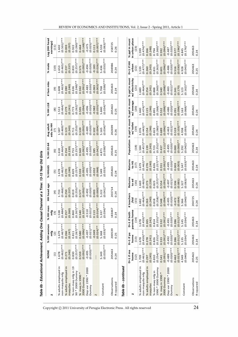
REVIEW OF ECONOMICS AND INSTITUTIONS, Vol. 2, Issue 2 - Spring 2011, Article 1
Tabl
e6b
-Edu
catio
nalA
chie
vem
ent,
Add
ing
One
Cau
salC
hann
elat
aTi
me:
13-1
5Ye
arO
ldG
irls
13-1
5 y
ear o
ld g
irls
Z
NO
NE
%
HH
wo
me
n
mfg
%
HH
me
n
mfg
H
H h
ea
d a
ge
%
HH
≥6
5
% H
H 2
2-6
4
Av
g a
du
lt
ed
u i
n H
H
% H
H ≤
18
#
fa
m m
bs
% m
ale
Lo
g (
HH
he
ad
e
arn
ing
s)
(1)
(2)
(3)
(4)
(5)
(6)
(7)
(8)
(9)
(10
) (1
1)
% a
du
lts
em
plo
ye
d i
n
no
n-m
aq
uil
a m
fg
1.6
78
(0
.46
2)*
**
1
.67
9
(0.4
67
)**
*
1.5
38
(0
.48
4)*
**
1
.73
3
(0.4
66
)**
*
1.6
78
(0
.46
2)*
**
1
.61
8
(0.4
64
)**
*
1.5
87
(0
.46
9)*
**
1
.51
3
(0.4
64
)**
*
1.6
08
(0
.46
3)*
**
1
.65
3
(0.4
65
)**
*
1.6
02
(0
.50
1)*
**
% a
du
lts
em
plo
ye
d i
n
ma
qu
ila
s 0
.27
1
(0.2
40
) 0
.26
6
(0.2
47
) 0
.25
7
(0.2
60
) 0
.25
0
(0.2
37
) 0
.27
0
(0.2
40
) 0
.25
4
(0.2
39
) 0
.12
3
(0.2
43
) 0
.27
9
(0.2
41
) 0
.28
0
(0.2
40
) 0
.23
7
(0.2
37
) 0
.00
3
(0.2
97
)
% n
on
-ma
q m
fg i
n 1
99
0 *
20
00
Du
mm
y
0.8
30
(0
.25
7)*
**
0
.81
1
(0.2
67
)**
*
0.8
60
(0
.26
7)*
**
0
.81
9
(0.2
55
)**
*
0.8
29
(0
.25
7)*
**
0
.75
3
(0.2
57
)**
*
0.7
11
(0
.25
3)*
**
0
.77
3
(0.2
62
)**
*
0.6
36
(0
.24
8)*
*
0.8
33
(0
.25
7)*
**
0
.92
2
(0.2
60
)**
*
%
ma
q i
n 1
99
0 *
2
00
0 D
um
my
0.5
59
(0
.09
2)*
**
0
.58
0
(0.0
96
)**
*
0.5
40
(0
.10
7)*
**
0
.57
7
(0.0
93
)**
*
0.5
59
(0
.09
2)*
**
0
.56
9
(0.0
92
)**
*
0.5
39
(0
.09
3)*
**
0
.59
5
(0.0
94
)**
*
0.5
92
(0
.09
1)*
**
0
.57
1
(0.0
95
)**
*
0.4
64
(0
.14
8)*
**
De
p v
ar
19
90
* 2
00
0
Du
mm
y
-0.4
95
(0
.02
0)*
**
-0
.49
7
(0.0
21
)**
*
-0.5
10
(0
.02
1)*
**
-0
.49
2
(0.0
20
)**
*
-0.4
95
(0
.02
0)*
**
-0
.49
5
(0.0
20
)**
*
-0.4
89
(0
.02
0)*
**
-0
.49
6
(0.0
20
)**
*
-0.4
83
(0
.02
0)*
**
-0
.49
4
(0.0
20
)**
*
-0.4
75
(0
.02
5)*
**
Z
----
-0
.04
9
(0.0
24
)**
0
.11
3
(0.0
14
)**
*
0.0
03
(0
.00
0)*
**
-0
.03
2
(0.0
68
) 1
.28
5
(0.0
42
)**
*
0.1
02
(0
.00
4)*
**
-0
.98
2
(0.0
35
)**
*
-0.0
63
(0
.00
3)*
**
-0
.18
3
(0.0
26
)**
*
0.1
11
(0
.00
7)*
**
Co
nst
an
t 5
.34
9
(0.0
33
)**
*
5.3
68
(0
.03
3)*
**
5
.33
7
(0.0
34
)**
*
5.2
22
(0
.04
1)*
**
5
.34
9
(0.0
33
)**
*
4.8
71
(0
.03
8)*
**
5
.16
5
(0.0
34
)**
*
5.8
40
(0
.03
4)*
**
5
.76
8
(0.0
38
)**
*
5.4
36
(0
.03
3)*
**
4
.55
9
(0.0
63
)**
*
Ob
serv
ati
on
s 2
05
46
3
20
05
39
1
83
46
7
20
37
14
2
05
46
3
20
54
63
2
02
69
9
20
54
63
2
05
46
3
20
49
86
1
58
72
5
R-s
qu
are
d
0.2
4
0.2
5
0.2
4
0.2
4
0.2
4
0.2
5
0.2
6
0.2
5
0.2
4
0.2
4
0.2
6
Tabl
e6b
-con
tinue
d
13-1
5 y
ear
old
gir
ls c
onti
nued
:
Z
D=
1 i
f m
a
ho
me
D
=1
if
pa
h
om
e
D=
1 i
f b
oth
p
are
nts
ho
me
#
te
ach
ers
/k
id
Re
turn
s
to e
d
Re
turn
s
to H
S
Po
pu
lati
on
%
pp
l in
mu
ni
w/ t
oil
et
% p
pl
in m
un
i w
/ s
ew
ag
e
% p
pl
in m
un
i w
/ e
lectr
icit
y
D=
1 i
f H
H
urb
an
%
pp
l in
mu
ni
in u
rba
n p
lace
(1
2)
(13
) (1
4)
(15
) (1
6)
(17
) (1
8)
(19
) (2
0)
(21
) (2
2)
(23
)
% a
du
lts
em
plo
ye
d i
n
no
n-m
aq
uil
a m
fg
1.7
09
(0
.46
1)*
**
1
.67
8
(0.4
59
)**
*
1.6
78
(0
.45
9)*
**
1
.68
2
(0.4
64
)**
*
1.6
69
(0
.46
5)*
**
1
.67
9
(0.4
62
)**
*
1.5
84
(0
.45
7)*
**
1
.07
6
(0.4
43
)**
1
.44
0
(0.4
74
)**
*
1.6
80
(0
.46
4)*
**
1
.53
9
(0.4
77
)**
*
1.5
99
(0
.47
4)*
**
% a
du
lts
em
plo
ye
d i
n
ma
qu
ila
s 0
.29
7
(0.2
45
) 0
.27
8
(0.2
41
) 0
.26
5
(0.2
42
) 0
.26
3
(0.2
40
) 0
.27
3
(0.2
39
) 0
.27
6
(0.2
40
) 0
.13
9
(0.2
43
) 0
.15
4
(0.2
46
) 0
.11
5
(0.2
46
) 0
.25
4
(0.2
41
) 0
.26
0
(0.2
43
) 0
.26
6
(0.2
48
)
% n
on
-ma
q m
fg i
n
19
90
* 2
00
0 D
um
my
0.8
10
(0
.25
4)*
**
0
.82
6
(0.2
55
)**
*
0.8
14
(0
.25
5)*
**
0
.81
8
(0.2
58
)**
*
0.8
23
(0
.25
7)*
**
0
.82
6
(0.2
57
)**
*
0.7
23
(0
.25
2)*
**
0
.82
3
(0.2
80
)**
*
0.8
91
(0
.26
8)*
**
0
.88
8
(0.2
60
)**
*
0.8
31
(0
.26
3)*
**
0
.79
4
(0.2
60
)**
*
%
ma
q i
n 1
99
0 *
2
00
0 D
um
my
0.5
41
(0
.09
1)*
**
0
.53
3
(0.0
91
)**
*
0.5
32
(0
.09
1)*
**
0
.54
8
(0.0
94
)**
*
0.5
54
(0
.09
1)*
**
0
.55
1
(0.0
92
)**
*
0.4
37
(0
.11
2)*
**
0
.68
9
(0.0
96
)**
*
0.5
32
(0
.09
8)*
**
0
.54
0
(0.0
98
)**
*
0.6
01
(0
.09
6)*
**
0
.59
2
(0.0
94
)**
*
De
p v
ar
19
90
* 2
00
0
Du
mm
y
-0.4
89
(0
.02
0)*
**
-0
.49
2
(0.0
20
)**
*
-0.4
91
(0
.02
0)*
**
-0
.49
5
(0.0
20
)**
*
-0.4
97
(0
.02
1)*
**
-0
.49
5
(0.0
20
)**
*
-0.4
95
(0
.02
0)*
**
-0
.46
3
(0.0
22
)**
*
-0.4
86
(0
.02
0)*
**
-0
.48
3
(0.0
22
)**
*
-0.4
86
(0
.02
0)*
**
-0
.48
7
(0.0
20
)**
*
Z
0.4
62
(0
.02
3)*
**
0
.28
6
(0.0
12
)**
*
0.2
86
(0
.01
2)*
**
-0
.47
2
(0.6
64
) 0
.33
6
(0.8
81
) 0
.00
3
(0.0
03
) 0
.00
0
(0.0
00
)**
0
.51
9
(0.1
03
)**
*
0.2
91
(0
.09
8)*
**
0
.24
1
(0.1
70
) 0
.51
6
(0.0
30
)**
*
0.5
77
(0
.19
6)*
**
Co
nst
an
t 4
.94
9
(0.0
40
)**
*
5.1
35
(0
.03
4)*
**
5
.14
5
(0.0
34
)**
*
5.3
66
(0
.04
0)*
**
5
.32
7
(0.0
63
)**
*
5.3
47
(0
.03
3)*
**
5
.29
2
(0.0
42
)**
*
4.9
38
(0
.09
3)*
**
5
.16
3
(0.0
68
)**
*
5.1
23
(0
.16
2)*
**
4
.92
8
(0.0
43
)**
*
4.8
45
(0
.17
6)*
**
Ob
serv
ati
on
s 2
05
46
3
20
54
63
2
05
46
3
20
47
25
2
05
46
3
20
54
63
2
05
46
3
20
54
63
2
05
46
3
20
54
63
2
05
46
3
20
54
63
R-s
qu
are
d
0.2
5
0.2
4
0.2
4
0.2
4
0.2
4
0.2
4
0.2
4
0.2
4
0.2
4
0.2
4
0.2
5
0.2
4
Copyright c© 2011 University of Perugia Electronic Press. All rights reserved 24

Le Brun, Helper, Levine: The Effect of Industrialization on Children’s Education
Tabl
e6c
-Edu
catio
nalA
chie
vem
ent,
Add
ing
One
Cau
salC
hann
elat
aTi
me:
16-1
8Ye
arO
ldG
irls
16-1
8 y
ear o
ld g
irls
Z
NO
NE
%
HH
wo
me
n
mfg
%
HH
me
n m
fg
HH
he
ad
ag
e
% H
H≥
65
%
HH
22
-64
A
vg
ad
ult
e
du
in
HH
%
HH
≤1
8
# f
am
mb
s %
ma
le
Log
(H
H h
ea
d
ea
rnin
gs)
(1
) (2
) (3
) (4
) (5
) (6
) (7
) (8
) (9
) (1
0)
(11
)
% a
du
lts
em
plo
ye
d i
n
no
n-m
aq
uil
a m
fg
-0.6
70
(0
.81
5)
-0.2
14
(0
.84
3)
-0.8
71
(0
.80
6)
-0.3
41
(0
.85
6)
-0.6
59
(0
.81
4)
-0.7
64
(0
.81
2)
-0.4
78
(0
.78
6)
-1.0
17
(0
.81
0)
-0.6
66
(0
.81
6)
-0.4
97
(0
.81
2)
-0.6
08
(0
.84
4)
% a
du
lts
em
plo
ye
d i
n
ma
qu
ila
s -1
.09
5
(0.3
73
)**
*
-0.9
17
(0
.39
6)*
*
-1.0
49
(0
.37
2)*
**
-0
.85
7
(0.3
80
)**
-1
.08
0
(0.3
74
)**
*
-1.1
48
(0
.37
2)*
**
-1
.24
4
(0.3
67
)**
*
-1.1
37
(0
.38
3)*
**
-1
.05
8
(0.3
72
)**
*
-1.0
89
(0
.37
0)*
**
-1
.02
1
(0.4
05
)**
%
no
n-m
aq
mfg
in
1
99
0 *
20
00
Du
mm
y
0.8
23
(0
.38
2)*
*
0.9
03
(0
.37
7)*
*
0.6
03
(0
.39
9)
0.9
70
(0
.38
9)*
*
0.8
36
(0
.38
2)*
*
0.8
31
(0
.37
4)*
*
0.6
30
(0
.35
6)*
0
.86
2
(0.3
81
)**
0
.65
7
(0.3
81
)*
0.8
50
(0
.37
3)*
*
0.5
59
(0
.39
4)
%
ma
q i
n 1
99
0 *
2
00
0 D
um
my
0.6
39
(0
.24
1)*
**
0
.59
1
(0.2
53
)**
0
.48
7
(0.2
32
)**
0
.68
8
(0.2
43
)**
*
0.6
37
(0
.24
1)*
**
0
.64
1
(0.2
44
)**
*
0.4
87
(0
.24
5)*
*
0.8
00
(0
.24
7)*
**
0
.64
5
(0.2
52
)**
0
.63
5
(0.2
45
)**
*
0.3
12
(0
.26
1)
De
p v
ar
19
90
* 2
00
0
Du
mm
y
-0.3
00
(0
.01
8)*
**
-0
.30
4
(0.0
18
)**
*
-0.2
97
(0
.01
9)*
**
-0
.30
5
(0.0
18
)**
*
-0.3
00
(0
.01
8)*
**
-0
.30
9
(0.0
18
)**
*
-0.2
83
(0
.01
7)*
**
-0
.30
1
(0.0
18
)**
*
-0.2
95
(0
.01
9)*
**
-0
.29
5
(0.0
18
)**
*
-0.2
74
(0
.01
8)*
**
Z
----
-0
.37
4
(0.0
40
)**
*
0.0
06
(0
.02
7)
0.0
21
(0
.00
1)*
**
0
.43
4
(0.0
88
)**
*
2.2
98
(0
.05
5)*
**
0
.16
8
(0.0
06
)**
*
-1.9
63
(0
.04
9)*
**
-0
.05
8
(0.0
04
)**
*
-1.0
74
(0
.04
0)*
**
0
.24
4
(0.0
12
)**
*
Co
nst
an
t 6
.87
6
(0.0
51
)**
*
6.9
44
(0
.05
3)*
**
6
.86
4
(0.0
51
)**
*
5.8
78
(0
.06
2)*
**
6
.86
4
(0.0
51
)**
*
6.0
47
(0
.05
7)*
**
6
.51
5
(0.0
53
)**
*
7.8
33
(0
.05
1)*
**
7
.27
1
(0.0
56
)**
*
7.4
04
(0
.05
2)*
**
5
.06
7
(0.1
10
)**
*
Ob
serv
ati
on
s 1
91
95
5
18
34
02
1
71
87
9
19
01
23
1
91
95
5
19
19
55
1
83
02
7
19
19
55
1
91
95
5
19
11
67
1
43
69
8
R-s
qu
are
d
0.2
0
0.2
1
0.2
0
0.2
1
0.2
0
0.2
2
0.2
4
0.2
1
0.2
0
0.2
1
0.2
1
Tabl
e6c
-con
tinue
d
16-1
8 y
ear
old
gir
ls, conti
nued:
Z
D=
1 i
f m
a
ho
me
D
=1
if
pa
h
om
e
D=
1 i
f b
oth
p
are
nts
ho
me
#
te
ach
ers
/k
id
Re
turn
s
to e
d
Re
turn
s
to H
S
Po
pu
lati
on
%
pp
l in
mu
ni
w
/ t
oil
et
% p
pl
in m
un
i
w/ s
ew
ag
e
% p
pl
in m
un
i w
/ e
lectr
icit
y
D=
1 i
f H
H
urb
an
%
pp
l in
mu
ni
i n
urb
an
pla
ce
(1
2)
(13
) (1
4)
(15
) (1
6)
(17
) (1
8)
(19
) (2
0)
(21
) (2
2)
(23
)
% a
du
lts
em
plo
ye
d i
n
no
n-m
aq
uil
a m
fg
-0.3
23
(0
.79
1)
-0.5
27
(0
.79
3)
-0.5
75
(0
.79
1)
-0.6
71
(0
.81
5)
-0.6
38
(0
.82
9)
-0.6
71
(0
.81
4)
-0.6
16
(0
.82
9)
-1.1
24
(0
.80
4)
-1.1
15
(0
.78
2)
-0.5
71
(0
.82
0)
-0.8
62
(0
.80
6)
-0.7
70
(0
.82
7)
% a
du
lts
em
plo
ye
d i
n
ma
qu
ila
s -0
.82
3
(0.3
68
)**
-0
.98
9
(0.3
82
)**
*
-1.0
24
(0
.37
8)*
**
-1
.10
3
(0.3
74
)**
*
-1.0
95
(0
.37
6)*
**
-1
.11
2
(0.3
69
)**
*
-1.0
35
(0
.39
1)*
**
-1
.17
6
(0.3
85
)**
*
-1.4
38
(0
.40
6)*
**
-1
.12
7
(0.4
06
)**
*
-1.1
21
(0
.36
3)*
**
-1
.08
5
(0.3
76
)**
*
% n
on
-ma
q m
fg i
n
19
90
* 2
00
0 D
um
my
0.8
50
(0
.38
0)*
*
0.8
03
(0
.37
1)*
*
0.8
03
(0
.37
1)*
*
0.8
16
(0
.38
1)*
*
0.8
42
(0
.38
6)*
*
0.8
38
(0
.38
2)*
*
0.8
69
(0
.40
4)*
*
0.8
51
(0
.38
8)*
*
0.9
76
(0
.38
8)*
*
1.1
43
(0
.38
3)*
**
0
.84
4
(0.3
75
)**
0
.76
4
(0.3
75
)**
%
ma
q i
n 1
99
0 *
2
00
0 D
um
my
0.5
95
(0
.24
3)*
*
0.6
21
(0
.22
6)*
**
0
.63
0
(0.2
27
)**
*
0.6
31
(0
.24
3)*
**
0
.65
0
(0.2
41
)**
*
0.6
64
(0
.23
0)*
**
0
.69
2
(0.2
67
)**
*
0.7
65
(0
.24
8)*
**
0
.57
2
(0.2
50
)**
0
.57
8
(0.2
96
)*
0.7
24
(0
.25
6)*
**
0
.72
2
(0.2
63
)**
*
De
p v
ar
19
90
* 2
00
0
Du
mm
y
-0.3
00
(0
.01
7)*
**
-0
.29
9
(0.0
18
)**
*
-0.2
99
(0
.01
8)*
**
-0
.30
0
(0.0
18
)**
*
-0.2
98
(0
.01
8)*
**
-0
.30
1
(0.0
18
)**
*
-0.2
99
(0
.01
8)*
**
-0
.27
9
(0.0
19
)**
*
-0.2
79
(0
.01
8)*
**
-0
.26
5
(0.0
21
)**
*
-0.2
88
(0
.01
8)*
**
-0
.28
4
(0.0
18
)**
*
Z
1.1
27
(0
.02
7)*
**
0
.78
7
(0.0
17
)**
*
0.7
67
(0
.01
7)*
**
-0
.39
0
(1.5
18
) -0
.81
9
(1.1
55
) -0
.01
1
(0.0
04
)**
*
-0.0
00
(0
.00
0)
0.4
57
(0
.16
3)*
**
0
.68
9
(0.1
63
)**
*
1.1
13
(0
.37
8)*
**
1
.15
8
(0.0
46
)**
*
1.3
25
(0
.31
5)*
**
Co
nst
an
t 5
.98
4
(0.0
57
)**
*
6.3
41
(0
.05
3)*
**
6
.38
5
(0.0
53
)**
*
6.8
91
(0
.07
8)*
**
6
.92
9
(0.0
81
)**
*
6.8
80
(0
.05
1)*
**
6
.90
1
(0.0
59
)**
*
6.5
09
(0
.14
5)*
**
6
.42
6
(0.1
18
)**
*
5.8
27
(0
.35
4)*
**
5
.90
7
(0.0
65
)**
*
5.7
10
(0
.28
2)*
**
Ob
serv
ati
on
s 1
91
95
5
19
19
55
1
91
95
5
19
12
28
1
91
95
5
19
19
55
1
91
95
5
19
19
55
1
91
95
5
19
19
55
1
91
95
5
19
19
55
R-s
qu
are
d
0.2
3
0.2
2
0.2
2
0.2
0
0.2
0
0.2
0
0.2
0
0.2
0
0.2
0
0.2
0
0.2
2
0.2
0
http://www.rei.unipg.it/rei/article/view/31 25

REVIEW OF ECONOMICS AND INSTITUTIONS, Vol. 2, Issue 2 - Spring 2011, Article 1
Tabl
e7a
-Edu
catio
nalA
chie
vem
ent,
Add
ing
One
Cau
salC
hann
elat
aTi
me:
7-12
Year
Old
Boy
s
7-1
2 y
ear o
ld b
oys
Z
NO
NE
%
HH
wo
me
n
mfg
%
HH
me
n
mfg
H
H h
ea
d a
ge
%
HH
≥6
5
% H
H 2
2-6
4
Av
g a
du
lt e
du
in
HH
%
HH
≤1
8
# f
am
mb
s
% m
ale
Lo
g (
HH
he
ad
e
arn
ing
s)
(1)
(2)
(3)
(4)
(5)
(6)
(7)
(8)
(9)
(10
) (1
1)
% a
du
lts e
mp
loy
ed
in
no
n-m
aq
uil
a m
fg
1.6
29
(0
.41
1)*
**
1
.58
9
(0.4
07
)**
*
1.4
32
(0
.41
9)*
**
1
.60
6
(0.4
09
)**
*
1.6
29
(0
.41
1)*
**
1
.57
6
(0.4
14
)**
*
1.6
06
(0
.40
4)*
**
1
.55
1
(0.4
18
)**
*
1.5
14
(0
.41
0)*
**
1
.61
8
(0.4
12
)**
*
1.5
84
(0
.41
2)*
**
% a
du
lts e
mp
loy
ed
in
ma
qu
ila
s 1
.02
5
(0.2
63
)**
*
1.0
01
(0
.26
6)*
**
1
.03
8
(0.2
71
)**
*
1.0
10
(0
.26
1)*
**
1
.02
6
(0.2
62
)**
*
1.0
54
(0
.26
5)*
**
1
.01
4
(0.2
59
)**
*
1.0
37
(0
.26
8)*
**
1
.04
4
(0.2
67
)**
*
1.0
31
(0
.26
4)*
**
1
.04
7
(0.2
61
)**
*
% n
on
-ma
q m
fg i
n
19
90
* 2
00
0
Du
mm
y
0.4
57
(0
.21
4)*
*
0.4
48
(0
.21
3)*
*
0.4
45
(0
.21
7)*
*
0.4
66
(0
.21
4)*
*
0.4
57
(0
.21
4)*
*
0.4
12
(0
.21
3)*
0
.39
9
(0.2
09
)*
0.4
11
(0
.21
4)*
0
.34
9
(0.2
17
) 0
.46
2
(0.2
14
)**
0
.53
2
(0.2
21
)**
%
ma
q i
n 1
99
0 *
2
00
0 D
um
my
0.5
29
(0
.10
0)*
**
0
.53
6
(0.1
00
)**
*
0.5
11
(0
.10
4)*
**
0
.51
8
(0.1
00
)**
*
0.5
29
(0
.10
0)*
**
0
.53
5
(0.1
01
)**
*
0.4
91
(0
.09
8)*
**
0
.55
7
(0.1
02
)**
*
0.5
48
(0
.10
1)*
**
0
.52
4
(0.1
01
)**
*
0.5
00
(0
.10
5)*
**
De
p v
ar
19
90
*
20
00
Du
mm
y
-0.4
92
(0
.04
5)*
**
-0
.49
3
(0.0
45
)**
*
-0.4
95
(0
.04
6)*
**
-0
.49
0
(0.0
45
)**
*
-0.4
91
(0
.04
5)*
**
-0
.49
3
(0.0
45
)**
*
-0.4
72
(0
.04
5)*
**
-0
.49
4
(0.0
44
)**
*
-0.4
69
(0
.04
6)*
**
-0
.49
0
(0.0
45
)**
*
-0.4
43
(0
.04
8)*
**
Z
-0
.04
6
(0.0
11
)**
*
0.0
64
(0
.00
7)*
**
-0
.00
1
(0.0
00
)**
-0
.03
5
(0.0
45
) 0
.86
4
(0.0
25
)**
*
0.0
62
(0
.00
2)*
**
-0
.66
4
(0.0
24
)**
*
-0.0
45
(0
.00
1)*
**
0
.03
6
(0.0
15
)**
0
.05
2
(0.0
03
)**
*
Co
nsta
nt
1.9
19
(0
.02
8)*
**
1
.92
3
(0.0
28
)**
*
3.6
82
(0
.02
9)*
**
1
.94
8
(0.0
32
)**
*
1.9
19
(0
.02
8)*
**
1
.70
8
(0.0
29
)**
*
3.5
77
(0
.02
9)*
**
2
.39
1
(0.0
29
)**
*
2.3
12
(0
.02
9)*
**
1
.90
2
(0.0
28
)**
*
4.2
32
(0
.04
0)*
**
Ob
se
rva
tio
ns
35
34
13
3
47
94
1
32
05
68
3
50
69
1
35
34
13
3
53
41
3
35
07
52
3
53
41
3
35
34
13
3
53
12
1
28
32
40
R-s
qu
are
d
0.5
9
0.6
0
0.6
0
0.5
9
0.5
9
0.6
0
0.6
0
0.5
9
0.6
0
0.5
9
0.6
1
Tabl
e7a
-con
tinue
d
7-1
2 y
ear
old
boys, conti
nued:
Z
D=
1 i
f m
a
ho
me
D
=1
if
pa
h
om
e
D=
1 i
f b
oth
p
are
nts
ho
me
#
te
ach
ers
/k
id
Re
turn
s t
o
ed
R
etu
rns t
o
HS
P
op
ula
tio
n %
pp
l in
mu
ni
w/ t
oil
et
% p
pl
in m
un
i w
/ s
ew
ag
e
% p
pl
in m
un
i w
/ e
lectr
icit
y
D=
1 i
f H
H
urb
an
%
pp
l in
mu
ni
in
urb
an
pla
ce
(1
2)
(13
) (1
4)
(15
) (1
6)
(17
) (1
8)
(19
) (2
0)
(21
) (2
2)
(23
)
% a
du
lts
em
plo
ye
d
in n
on
-ma
qu
ila
mfg
1
.62
7
(0.4
09
)**
*
1.6
24
(0
.41
0)*
**
1
.62
0
(0.4
09
)**
*
1.6
27
(0
.41
0)*
**
1
.62
6
(0.4
12
)**
*
1.6
29
(0
.41
2)*
**
1
.58
5
(0.4
10
)**
*
1.6
58
(0
.41
5)*
**
1
.52
8
(0.4
26
)**
*
1.6
23
(0
.41
3)*
**
1
.58
6
(0.4
12
)**
*
1.5
69
(0
.41
4)*
**
% a
du
lts
em
plo
ye
d
in m
aq
uil
as
1.0
21
(0
.26
2)*
**
1
.02
9
(0.2
61
)**
*
1.0
26
(0
.26
0)*
**
1
.00
8
(0.2
58
)**
*
1.0
27
(0
.26
3)*
**
1
.04
0
(0.2
66
)**
*
0.9
63
(0
.26
3)*
**
1
.03
1
(0.2
62
)**
*
0.9
64
(0
.26
5)*
**
1
.02
2
(0.2
63
)**
*
1.0
26
(0
.26
5)*
**
1
.02
2
(0.2
68
)**
*
% n
on
-ma
q m
fg i
n
19
90
* 2
00
0 D
um
my
0.4
49
(0
.21
5)*
*
0.4
45
(0
.21
3)*
*
0.4
43
(0
.21
4)*
*
0.4
44
(0
.21
2)*
*
0.4
53
(0
.21
6)*
*
0.4
45
(0
.21
3)*
*
0.4
02
(0
.22
3)*
0
.45
6
(0.2
14
)**
0
.48
2
(0.2
17
)**
0
.46
7
(0.2
21
)**
0
.45
7
(0.2
15
)**
0
.43
9
(0.2
15
)**
%
ma
q i
n 1
99
0 *
2
00
0 D
um
my
0.5
28
(0
.10
0)*
**
0
.51
4
(0.1
00
)**
*
0.5
14
(0
.10
0)*
**
0
.51
4
(0.0
98
)**
*
0.5
27
(0
.10
1)*
**
0
.50
8
(0.1
04
)**
*
0.4
70
(0
.11
2)*
**
0
.52
4
(0.1
03
)**
*
0.5
21
(0
.10
0)*
**
0
.52
6
(0.1
01
)**
*
0.5
37
(0
.10
0)*
**
0
.54
8
(0.1
01
)**
*
De
p v
ar
19
90
* 2
00
0
Du
mm
y
-0.4
88
(0
.04
5)*
**
-0
.49
0
(0.0
45
)**
*
-0.4
89
(0
.04
5)*
**
-0
.49
0
(0.0
46
)**
*
-0.4
93
(0
.04
6)*
**
-0
.49
0
(0.0
45
)**
*
-0.4
87
(0
.04
6)*
**
-0
.49
4
(0.0
45
)**
*
-0.4
86
(0
.04
5)*
**
-0
.48
6
(0.0
53
)**
*
-0.4
83
(0
.04
5)*
**
-0
.48
3
(0.0
46
)**
*
Z
0.1
31
(0
.01
0)*
**
0
.12
0
(0.0
07
)**
*
0.1
26
(0
.00
7)*
**
-0
.84
4
(0.7
40
) 0
.21
0
(0.7
36
) 0
.00
8
(0.0
03
)**
*
0.0
00
(0
.00
0)
-0.0
21
(0
.07
6)
0.1
10
(0
.08
5)
0.0
42
(0
.20
1)
0.1
87
(0
.01
6)*
**
0
.31
6
(0.1
50
)**
Co
nst
an
t 1
.79
6
(0.0
29
)**
*
1.8
13
(0
.02
8)*
**
1
.81
0
(0.0
28
)**
*
3.7
03
(0
.04
0)*
**
1
.90
5
(0.0
55
)**
*
1.9
16
(0
.02
8)*
**
1
.89
2
(0.0
31
)**
*
1.9
35
(0
.06
6)*
**
1
.84
9
(0.0
61
)**
*
1.8
80
(0
.18
8)*
**
1
.77
3
(0.0
31
)**
*
1.6
44
(0
.13
7)*
**
Ob
serv
ati
on
s 3
53
41
3
35
34
13
3
53
41
3
35
21
61
3
53
41
3
35
34
13
3
53
41
3
35
34
13
3
53
41
3
35
34
13
3
53
41
3
35
34
13
R-s
qu
are
d
0.5
9
0.5
9
0.5
9
0.5
9
0.5
9
0.5
9
0.5
9
0.5
9
0.5
9
0.5
9
0.5
9
0.5
9
Copyright c© 2011 University of Perugia Electronic Press. All rights reserved 26

Le Brun, Helper, Levine: The Effect of Industrialization on Children’s Education
Tabl
e7b
-Edu
catio
nalA
chie
vem
ent,
Add
ing
One
Cau
salC
hann
elat
aTi
me:
13-1
5Ye
arO
ldB
oys
13-1
5 y
ear o
ld b
oys
Z
NO
NE
%
HH
wo
me
n
mfg
%
HH
me
n
mfg
H
H h
ea
d a
ge
%
HH
≥6
5
% H
H 2
2-6
4
Av
g a
du
lt
ed
u i
n H
H
% H
H ≤
18
#
fa
m m
bs
% m
ale
Lo
g (
HH
he
ad
e
arn
ing
s)
(1
) (2
) (3
) (4
) (5
) (6
) (7
) (8
) (9
) (1
0)
(11
)
% a
du
lts
em
plo
ye
d i
n
no
n-m
aq
uil
a m
fg
1.0
35
(0
.57
5)*
1
.07
2
(0.5
68
)*
1.0
09
(0
.55
5)*
1
.02
8
(0.5
77
)*
1.0
24
(0
.57
6)*
0
.96
8
(0.5
63
)*
0.9
89
(0
.53
3)*
0
.98
7
(0.5
62
)*
0.9
82
(0
.56
1)*
1
.00
0
(0.5
78
)*
0.8
19
(0
.61
5)
% a
du
lts
em
plo
ye
d i
n
ma
qu
ila
s 0
.89
0
(0.3
65
)**
0
.84
1
(0.3
67
)**
0
.97
0
(0.3
62
)**
*
0.9
05
(0
.36
9)*
*
0.8
91
(0
.36
6)*
*
0.8
87
(0
.36
4)*
*
0.8
27
(0
.35
9)*
*
0.8
88
(0
.36
7)*
*
0.9
08
(0
.36
0)*
*
0.8
63
(0
.37
1)*
*
1.0
47
(0
.40
0)*
**
%
no
n-m
aq
mfg
in
1
99
0 *
20
00
Du
mm
y
0.4
11
(0
.31
6)
0.3
82
(0
.30
3)
0.4
43
(0
.31
3)
0.3
46
(0
.31
4)
0.4
07
(0
.31
6)
0.2
56
(0
.31
2)
0.1
11
(0
.29
9)
0.3
44
(0
.31
7)
0.1
54
(0
.30
0)
0.4
10
(0
.31
6)
0.4
49
(0
.33
9)
%
ma
q i
n 1
99
0 *
2
00
0 D
um
my
0.8
41
(0
.15
6)*
**
0
.89
4
(0.1
56
)**
*
0.7
97
(0
.15
6)*
**
0
.81
2
(0.1
57
)**
*
0.8
38
(0
.15
6)*
**
0
.82
8
(0.1
62
)**
*
0.7
46
(0
.15
6)*
**
0
.89
3
(0.1
61
)**
*
0.8
47
(0
.15
6)*
**
0
.85
4
(0.1
59
)**
*
0.7
06
(0
.16
4)*
**
D
ep
va
r 1
99
0 *
20
00
D
um
my
-0.4
01
(0
.02
6)*
**
-0
.40
1
(0.0
24
)**
*
-0.4
14
(0
.02
6)*
**
-0
.39
8
(0.0
26
)**
*
-0.4
01
(0
.02
6)*
**
-0
.40
4
(0.0
25
)**
*
-0.3
89
(0
.02
4)*
**
-0
.40
3
(0.0
26
)**
*
-0.3
86
(0
.02
6)*
**
-0
.39
8
(0.0
26
)**
*
-0.3
80
(0
.02
7)*
**
Z
----
-0
.07
6
(0.0
23
)**
*
0.1
23
(0
.01
4)*
**
-0
.00
0
(0.0
00
) -0
.22
9
(0.0
64
)**
*
1.5
12
(0
.04
1)*
**
0
.13
3
(0.0
03
)**
*
-1.0
53
(0
.03
7)*
**
-0
.08
0
(0.0
03
)**
*
-0.0
78
(0
.02
6)*
**
0
.12
0
(0.0
06
)**
*
Co
nst
an
t 4
.94
8
(0.0
38
)**
*
4.9
47
(0
.03
9)*
**
4
.92
9
(0.0
38
)**
*
4.9
62
(0
.04
6)*
**
4
.94
9
(0.0
38
)**
*
4.5
99
(0
.04
0)*
**
4
.75
5
(0.0
38
)**
*
5.7
03
(0
.04
2)*
**
5
.66
5
(0.0
43
)**
*
4.9
87
(0
.03
9)*
**
4
.11
6
(0.0
62
)**
*
Ob
serv
ati
on
s 2
04
66
8
19
98
87
1
83
53
6
20
30
80
2
04
66
8
20
46
68
2
02
35
7
20
46
68
2
04
66
8
20
42
29
1
57
94
4
R-s
qu
are
d
0.2
3
0.2
3
0.2
3
0.2
3
0.2
3
0.2
4
0.2
5
0.2
3
0.2
3
0.2
3
0.2
4
Tabl
e7b
-con
tinue
d
13-1
5 y
ear
old
boys, conti
nued:
Z
D=
1 i
f m
a
ho
me
D
=1
if
pa
h
om
e
D=
1 i
f b
oth
p
are
nts
ho
me
#
te
ach
ers
/k
id
Re
turn
s
to e
d
to H
S
R
etu
rns
P
op
ula
tio
n
% p
pl
in m
un
i
w/ t
oil
et
% p
pl
in m
un
i % p
pl i
n m
un
i w
/ s
ew
ag
e w
/ e
lectr
icit
y D
=1
if
HH
u
rba
n
% p
pl
in m
un
i i
n u
rba
n p
lace
(12
) (1
3)
(14
) (1
5)
(16
) (1
7)
(18
) (1
9)
(20
) (2
1)
(22
) (2
3)
% a
du
lts
em
plo
ye
d i
n
no
n-m
aq
uil
a m
fg
0.9
84
(0
.57
7)*
1
.05
7
(0.5
77
)*
1.0
33
(0
.57
8)*
1
.03
6
(0.5
72
)*
1.0
34
(0
.58
2)*
1
.03
5
(0.5
75
)*
1.0
03
(0
.56
9)*
1
.03
7
(0.5
83
)*
0.7
23
(0
.57
7)
1.0
37
(0
.57
7)*
0
.96
0
(0.5
79
)*
0.9
80
(0
.58
1)*
% a
du
lts
em
plo
ye
d i
n
ma
qu
ila
s 0
.88
8
(0.3
65
)**
0
.90
2
(0.3
64
)**
0
.89
4
(0.3
65
)**
0
.87
0
(0.3
63
)**
0
.89
0
(0.3
65
)**
0
.88
4
(0.3
64
)**
0
.84
7
(0.3
74
)**
0
.89
0
(0.3
61
)**
0
.68
5
(0.3
72
)*
0.8
84
(0
.36
8)*
*
0.8
40
(0
.37
6)*
*
0.8
85
(0
.37
0)*
*
% n
on
-ma
q m
fg i
n
19
90
* 2
00
0 D
um
my
0.4
22
(0
.31
6)
0.4
05
(0
.31
7)
0.3
92
(0
.31
7)
0.3
95
(0
.31
5)
0.4
10
(0
.31
5)
0.4
15
(0
.31
6)
0.3
75
(0
.33
3)
0.4
11
(0
.31
6)
0.4
91
(0
.33
1)
0.4
33
(0
.31
7)
0.4
04
(0
.31
8)
0.3
87
(0
.31
5)
%
ma
q i
n 1
99
0 *
2
00
0 D
um
my
0.8
46
(0
.15
7)*
**
0
.82
9
(0.1
58
)**
*
0.8
27
(0
.15
7)*
**
0
.82
4
(0.1
55
)**
*
0.8
40
(0
.15
4)*
**
0
.84
9
(0.1
55
)**
*
0.8
00
(0
.17
3)*
**
0
.84
0
(0.1
56
)**
*
0.8
06
(0
.16
0)*
**
0
.83
4
(0.1
56
)**
*
0.8
78
(0
.15
8)*
**
0
.86
4
(0.1
60
)**
*
De
p v
ar
19
90
* 2
00
0
Du
mm
y
-0.3
97
(0
.02
6)*
**
-0
.39
7
(0.0
26
)**
*
-0.3
95
(0
.02
6)*
**
-0
.40
0
(0.0
26
)**
*
-0.4
01
(0
.02
7)*
**
-0
.40
1
(0.0
26
)**
*
-0.4
00
(0
.02
6)*
**
-0
.40
1
(0.0
27
)**
*
-0.3
89
(0
.02
7)*
**
-0
.39
6
(0.0
28
)**
*
-0.3
93
(0
.02
6)*
**
-0
.39
5
(0.0
27
)**
*
Z
0.3
01
(0
.01
7)*
**
0
.23
8
(0.0
13
)**
*
0.2
55
(0
.01
2)*
**
-0
.75
8
(0.8
60
) 0
.03
2
(0.9
54
) -0
.00
4
(0.0
03
) 0
.00
0
(0.0
00
) -0
.00
2
(0.1
20
) 0
.38
6
(0.1
03
)**
*
0.0
90
(0
.19
1)
0.5
41
(0
.03
1)*
**
0
.38
6
(0.2
07
)*
Co
nst
an
t 4
.66
8
(0.0
43
)**
*
4.7
41
(0
.03
9)*
**
4
.73
2
(0.0
40
)**
*
4.9
76
(0
.04
8)*
**
4
.94
6
(0.0
67
)**
*
4.9
49
(0
.03
8)*
**
4
.93
0
(0.0
48
)**
*
4.9
50
(0
.10
6)*
**
4
.70
2
(0.0
78
)**
*
4.8
63
(0
.18
4)*
**
4
.52
1
(0.0
48
)**
*
4.6
11
(0
.18
4)*
**
Ob
serv
ati
on
s 2
04
66
8
20
46
68
2
04
66
8
20
38
76
2
04
66
8
20
46
68
2
04
66
8
20
46
68
2
04
66
8
20
46
68
2
04
66
8
20
46
68
R-s
qu
are
d
0.2
3
0.2
3
0.2
3
0.2
3
0.2
3
0.2
3
0.2
3
0.2
3
0.2
3
0.2
3
0.2
3
0.2
3
http://www.rei.unipg.it/rei/article/view/31 27
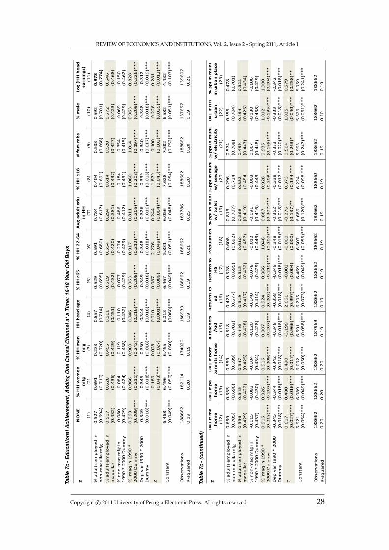
REVIEW OF ECONOMICS AND INSTITUTIONS, Vol. 2, Issue 2 - Spring 2011, Article 1
Tabl
e7c
-Edu
catio
nalA
chie
vem
ent,
Add
ing
One
Cau
salC
hann
elat
aTi
me:
16-1
8Ye
arO
ldB
oys
16-1
8 y
ear o
ld b
oys
Z
NO
NE
%
HH
wo
me
n
mfg
%
HH
me
n
mfg
H
H h
ea
d a
ge
%
HH
≥6
5
% H
H 2
2-6
4
Av
g a
du
lt e
du
in
HH
%
HH
≤1
8
# f
am
mb
s
% m
ale
Lo
g (
HH
he
ad
e
arn
ing
s)
(1
) (2
) (3
) (4
) (5
) (6
) (7
) (8
) (9
) (1
0)
(11
)
% a
du
lts
em
plo
ye
d i
n
no
n-m
aq
uil
a m
fg
0.5
27
(0
.69
4)
0.6
91
(0
.71
0)
0.2
33
(0
.72
0)
0.6
57
(0
.71
4)
0.5
29
(0
.69
5)
0.5
91
(0
.68
0)
0.7
84
(0
.61
7)
0.4
04
(0
.69
1)
0.5
33
(0
.66
8)
0.5
92
(0
.70
1)
0.9
73
(0
.77
4)
% a
du
lts
em
plo
ye
d i
n
ma
qu
ila
s 0
.51
7
(0.4
32
) 0
.62
8
(0.4
36
) 0
.45
5
(0.4
29
) 0
.61
1
(0.4
51
) 0
.51
9
(0.4
32
) 0
.55
4
(0.4
20
) 0
.29
4
(0.3
81
) 0
.61
4
(0.4
37
) 0
.52
0
(0.4
27
) 0
.57
2
(0.4
23
) 0
.54
6
(0.4
68
)
% n
on
-ma
q m
fg i
n
19
90
* 2
00
0 D
um
my
-0.0
80
(0
.42
9)
-0.0
84
(0
.42
4)
-0.1
19
(0
.43
8)
-0.1
10
(0
.43
2)
-0.0
77
(0
.42
9)
-0.2
74
(0
.42
9)
-0.4
86
(0
.41
2)
-0.1
84
(0
.43
1)
-0.3
54
(0
.41
5)
-0.0
69
(0
.42
9)
-0.1
50
(0
.46
2)
%
ma
q i
n 1
99
0 *
2
00
0 D
um
my
0.9
63
(0
.20
9)*
**
0
.96
6
(0.2
11
)**
*
0.9
00
(0
.24
2)*
**
0
.94
6
(0.2
16
)**
*
0.9
63
(0
.20
8)*
**
0
.91
7
(0.2
12
)**
*
0.8
11
(0
.20
5)*
**
1
.06
0
(0.2
08
)**
*
1.0
14
(0
.19
7)*
**
0
.96
3
(0.2
09
)**
*
0.8
28
(0
.22
6)*
**
De
p v
ar
19
90
* 2
00
0
Du
mm
y
-0.3
49
(0
.01
8)*
**
-0
.34
5
(0.0
18
)**
*
-0.3
50
(0
.01
8)*
**
-0
.34
4
(0.0
18
)**
*
-0.3
49
(0
.01
8)*
**
-0
.34
8
(0.0
18
)**
*
-0.3
26
(0
.01
6)*
**
-0
.33
9
(0.0
18
)**
*
-0.3
40
(0
.01
7)*
**
-0
.34
8
(0.0
18
)**
*
-0.3
12
(0
.01
9)*
**
Z
-0
.18
9
(0.0
43
)**
*
0.0
28
(0
.02
7)
0.0
10
(0
.00
1)*
**
0
.08
7
(0.0
89
) 2
.27
6
(0.0
49
)**
*
0.2
44
(0
.00
4)*
**
-1
.87
9
(0.0
45
)**
*
-0.1
00
(0
.00
3)*
**
-0
.22
6
(0.0
35
)**
*
0.2
81
(0
.01
2)*
**
Co
nst
an
t 6
.46
8
(0.0
49
)**
*
6.4
96
(0
.05
0)*
**
6
.49
5
(0.0
50
)**
*
6.0
13
(0
.06
0)*
**
6
.46
7
(0.0
49
)**
*
5.8
31
(0
.05
1)*
**
6
.05
6
(0.0
48
)**
*
7.6
28
(0
.05
4)*
**
7
.30
2
(0.0
52
)**
*
6.5
82
(0
.05
1)*
**
4
.43
2
(0.1
07
)**
*
Ob
serv
ati
on
s 1
88
66
2
18
21
14
1
74
02
0
18
69
33
1
88
66
2
18
86
62
1
83
78
6
18
86
62
1
88
66
2
18
76
57
1
39
60
7
R-s
qu
are
d
0.1
9
0.2
0
0.1
9
0.1
9
0.1
9
0.2
1
0.2
5
0.2
0
0.2
0
0.1
9
0.2
1
Tabl
e7c
-(co
ntin
ued)
Z
D=
1 i
f m
a
ho
me
D
=1
if
pa
h
om
e
D=
1 i
f b
oth
p
are
nts
ho
me
#
te
ach
ers
/k
id
Re
turn
s t
o
ed
R
etu
rns t
o
HS
P
op
ula
tio
n
% p
pl
in m
un
i w
/ t
oil
et
% p
pl
in m
un
i w
/ s
ew
ag
e
% p
pl
in m
un
i w
/ e
lectr
icit
y
D=
1 i
f H
H
urb
an
%
pp
l in
mu
ni
in u
rba
n p
lace
(12
) (1
3)
(14
) (1
5)
(16
) (1
7)
(18
) (1
9)
(20
) (2
1)
(22
) (2
3)
% a
du
lts
em
plo
ye
d i
n
no
n-m
aq
uil
a m
fg
0.6
59
(0
.70
5)
0.5
55
(0
.69
6)
0.5
89
(0
.69
9)
0.5
18
(0
.70
2)
0.4
23
(0
.67
7)
0.5
28
(0
.69
5)
0.6
08
(0
.69
2)
0.8
13
(0
.70
7)
0.2
96
(0
.72
4)
0.5
74
(0
.70
8)
0.3
55
(0
.70
4)
0.4
78
(0
.70
1)
% a
du
lts
em
plo
ye
d i
n
ma
qu
ila
s 0
.55
6
(0.4
29
) 0
.54
5
(0.4
22
) 0
.54
7
(0.4
25
) 0
.44
6
(0.4
28
) 0
.51
9
(0.4
17
) 0
.51
5
(0.4
32
) 0
.61
0
(0.4
57
) 0
.56
8
(0.4
19
) 0
.33
2
(0.4
54
) 0
.49
9
(0.4
43
) 0
.49
4
(0.4
25
) 0
.52
2
(0.4
34
)
% n
on
-ma
q m
fg i
n
19
90
* 2
00
0 D
um
my
-0.1
15
(0
.43
7)
-0.0
83
(0
.43
0)
-0.1
04
(0
.43
4)
-0.1
20
(0
.42
8)
-0.1
40
(0
.41
4)
-0.0
78
(0
.42
9)
-0.0
12
(0
.44
3)
-0.0
91
(0
.41
6)
-0.0
03
(0
.44
3)
0.0
67
(0
.44
8)
-0.1
30
(0
.43
8)
-0.1
06
(0
.42
9)
%
ma
q i
n 1
99
0 *
2
00
0 D
um
my
0.9
15
(0
.21
3)*
**
0
.92
6
(0.2
07
)**
*
0.9
15
(0
.20
9)*
**
0
.90
7
(0.2
07
)**
*
0.9
24
(0
.20
2)*
**
0
.96
6
(0.2
10
)**
*
1.0
46
(0
.20
0)*
**
0
.88
7
(0.2
07
)**
*
0.9
28
(0
.20
9)*
**
0
.93
6
(0.1
95
)**
*
1.0
12
(0
.19
5)*
**
1
.00
0
(0.2
04
)**
*
De
p v
ar
19
90
* 2
00
0
Du
mm
y
-0.3
45
(0
.01
8)*
**
-0
.34
4
(0.0
18
)**
*
-0.3
42
(0
.01
8)*
**
-0
.34
8
(0.0
18
)**
*
-0.3
58
(0
.01
8)*
**
-0
.34
9
(0.0
18
)**
*
-0.3
48
(0
.01
8)*
**
-0
.36
2
(0.0
18
)**
*
-0.3
38
(0
.01
7)*
**
-0
.33
3
(0.0
20
)**
*
-0.3
33
(0
.01
8)*
**
-0
.34
2
(0.0
18
)**
*
Z
0.6
17
(0
.02
7)*
**
0
.48
0
(0.0
16
)**
*
0.4
90
(0
.01
7)*
**
-3
.19
9
(0.9
66
)**
*
2.6
61
(0
.99
7)*
**
-0
.00
2
(0.0
04
) -0
.00
0
(0.0
00
) -0
.27
6
(0.1
37
)**
0
.37
3
(0.1
34
)**
*
0.5
04
(0
.26
3)*
1
.03
5
(0.0
40
)**
*
0.5
79
(0
.25
8)*
*
Co
nst
an
t 5
.92
1
(0.0
54
)**
*
6.0
89
(0
.04
9)*
**
6
.09
2
(0.0
50
)**
*
6.5
91
(0
.05
8)*
**
6
.29
5
(0.0
73
)**
*
6.4
69
(0
.04
9)*
**
6
.50
7
(0.0
55
)**
*
6.6
89
(0
.12
0)*
**
6
.22
4
(0.0
98
)**
*
5.9
93
(0
.24
7)*
**
5
.62
9
(0.0
61
)**
*
5.9
59
(0
.24
1)*
**
Ob
serv
ati
on
s 1
88
66
2
18
86
62
1
88
66
2
18
79
69
1
88
66
2
18
86
62
1
88
66
2
18
86
62
1
88
66
2
18
86
62
1
88
66
2
18
86
62
R-s
qu
are
d
0.2
0
0.2
0
0.2
0
0.1
9
0.1
9
0.1
9
0.1
9
0.1
9
0.1
9
0.1
9
0.2
0
0.1
9
Copyright c© 2011 University of Perugia Electronic Press. All rights reserved 28

Le Brun, Helper, Levine: The Effect of Industrialization on Children’s Education
To the extent that caring for household children is a burden that allhousehold women share, the negative impact that number of women inmanufacturing has on children’s outcomes is understandable. Of the manyjobs women occupy in Mexico, working in a factory is among the likeliestto require the woman’s separation from children of the household (this isin contrast to jobs such as, for example, shop keeper, artisan, or maid). It istherefore possible, that the more household females are employed in man-ufacturing, the fewer disciplinarians the children have to take care of them,ensure they do their homework and go to school.20
We have also undertaken the above analysis separating boys from girls(in results available upon request), and we find that among 16-18 year old inparticular, it is the girls who are most strikingly affected by the gender com-position of the household: the more women there are in the household, thebetter the educational outcomes of 16-18 year old girls. We also find that thegreater the number of household adult females employed in manufacturing,the worse the educational outcomes for 16-18 year old girls. These findingsare rather intuitive: the closest substitute for women in household choresare 16-18 year old girls. The more women the household has, and the fewerof these women that are occupied with the strict schedule of a manufactur-ing job, the less 16-18 year old girls in the household will have to assume thewomen’s responsibilities (cleaning, cooking, caring for younger children).Surprisingly though, 16-18 year old girls whose own mother works in man-ufacturing have better educational outcomes than those girls whose motherlives with them but does not work in manufacturing. For this finding, wehave no intuitive explanation.
In results not shown, we limit the sample to children whose father is athome, in order to be able to include a dummy for paternal manufacturingemployment in the regression. When we do this, results change: paternalmanufacturing employment is always associated with better children’s out-comes: if a child’s father is employed in manufacturing, that child is like-lier to be enrolled in school and not to work, and will have higher averagenumber of school years completed, regardless of age. In those regressionswhich include a dummy for paternal manufacturing employment, the im-pact of other household males’ manufacturing employment on children’soutcomes is negative: the more other men in the household (not the child’sfather) are employed in manufacturing, the lower the likelihood that thechild is enrolled in school, the lower his school years attained, and the morelikely he is to work. It is possible that in households with many males em-ployed in manufacturing, children, following a sort of path dependence,
20 If this “discipline vacuum” story is true, we might expect it to hit children in maquila-rich municipios particularly hard, because maquiladoras are more intense in female laborthan other manufacturing is. This claim would be verified if the coefficient on %MAQm
were “less negative” in the school attainment regressions once we control for “D=1 if maemployed in MFG”. This is in fact the case, though not in a statistically significant sense.
http://www.rei.unipg.it/rei/article/view/31 29

REVIEW OF ECONOMICS AND INSTITUTIONS, Vol. 2, Issue 2 - Spring 2011, Article 1
perceive manufacturing as the only job open to them, and act accordingly(dropping out of school, starting to work young, etc.). If this is the case, wemight expect these results to be stronger for boys, who are bound to feelmore “identified” with the men in the household than girls are. When wesplit the sample up by gender, we do find that the impact of non-paternalmale manufacturing employment is much stronger on boys’ likelihood ofworking than on girls, supporting our hypothesis.
5 Conclusion
Our analysis suggests that while non-maquila manufacturing and maqui-ladora employment are accompanied by small early improvements in schoolyears completed, these gains in educational attainment are erased by thetime children reach 16 years of age. In particular, girls aged 16-18 have lesseducation, the more maquiladora employment there is in their municipio.Despite a decline soon after the 2000 Census, employment in maquilas re-mains a key source of income and exports for Mexico. Given their centralrole in Mexican industrialization, it is concerning that maquiladoras may actto deter older girls’ educational attainment, whether it be by imposing morehousehold responsibilities on them (as their grown-up counterparts join themaquila workforce) or by pushing them into the maquila sector themselves.Maquilas began in the late 1990s to include more skill-intensive activities(Carrillo et. al., 1998; Carrillo and Hualde, 1996). Such upgrading is neces-sary to compete with even lower wages in China and India, but it remainsto be seen if the new focus towards more skill-intensive activities will gen-erate enough demand for an educated work force to benefit children’s andin particular girls’ educational outcomes in the long run.
It is possible that maquilas contribute to a low-education trap for Mex-ico (Tendler, 2002). The purpose of the maquila program was to createjobs, not upgrading — but by increasing the opportunity costs of stayingin school, maquilas may close off some development paths. As a UnitedNations report found, “transnational corporations bring technology appro-priate to existing education levels—they do not invest in improving thislevel”(UNCTAD, 2001, quoted in Hualde, 2001a). Thus, when other nationscan provide low-skilled labor more cheatly, multinationals shut their doorsand go elsewhere—they do not invest in creating a higher-skilled work forcein the first country.
It is interesting to compare the effects of industrialization on educationwith those of another program implemented around the same time—theProgresa/Oportunidades program, which paid families $6-10 for each monththeir child consistently attended school (Skoufias and Parker, 2001). Thisfederal government program served about 40% of the royal population.Careful studies comparing treatment and control groups found that the pro-gram increased educational attainment in primary grades by 10%. For our
Copyright c© 2011 University of Perugia Electronic Press. All rights reserved 30

Le Brun, Helper, Levine: The Effect of Industrialization on Children’s Education
population, that would lead to about about 15 weeks increased educationalattainment—vastly more than the one week (later reversed for girls) thatoccurred when maquila employment doubled in Mexico during the 1990s.
Some aspects of the Mexican experience allow us to tease out relation-ships that are of broader theoretical interest. We are able to rule tut re-verse causality in plant location; firms do not locate plants based on higheducation early in our period. In addition, national financing of schoolsmeans that manufacturing growth in a particular municipio does not bringincreased taxes that would increase supply of education in that one area.Thus, our case allows us to shed light on how different kinds of manufac-turing affect the demand for education.
Mexico has quite good data on its export processing zones (maquilas)allowing us to separate out different forms of foreign direct investment andtheir impacts on investment in children. The well–documented preferenceof maquila employers for women (and for other manufacturers to hire men)allows us no look at the role of labor income in intra-family bargaining. Ourfindings are not consistent with the “unitary” model of the household: chil-dren’s outcomes depend a great deal on which parent gets a manufacturingjob, and whether they are the same sex as that parent. When men get jobsin manufacturing, boys’ education benefits; girls’ education also benefits,but less strongly. When women get jobs in manufacturing, girls’ educationsuffers, while teenage boys’ benefits.
In addition, we separate out the impacts of industrialization on educa-tional attainment at different ages and by boys and girls.
The story that emerges is that manufacturing does appear to increasedemand for primary education, perhaps because of (small) increases in in-come, or to meet the maquilas’ education requirements. Neither type ofmanufacturing has the expected positive effects on infrastructure (such assewage), perhaps because these investments are financed nationally. Indus-trialization has a negative (though insignificant) impact on skill premia. Theeducation effect is weaker for maquiladoras than for other manufacturing,for two reasons we can identify. First, the income effect is less positive.Second, maquiladoras are more likely to hire women, and the impact of awoman in the household working in manufacturing is negative.
The effect of maquilas in a municipio turns negative for high-schoolgirls. This effect is consistent with a rising opportunity cost of staying inschool for these young women, both because of the absence of their moth-ers and of their own ability to get these jobs.
These results suggest that foreign investment, if it is focused on assembly-intensive manufacturing, does not necessarily increase returns to educa-tion or the overall demand for education. Moreover, providing income towomen does not necessarily increase investments in children, if obtainingthe income requires women to leave the household and does not providesubstitutes for women labor in the home.
http://www.rei.unipg.it/rei/article/view/31 31

REVIEW OF ECONOMICS AND INSTITUTIONS, Vol. 2, Issue 2 - Spring 2011, Article 1
References
Barajas Ma. del Rosıo, E., Almaraz, A.A., Carrillo, J.V., Contreras, O.,Hualde, A.A. & Rodriguez, C. (2004). Industria Maquiladora en Mexico: Per-spectivas del Aprendizaje Tecnologico-Organizacional y Escalamiento Industrial.Tijuana, Baja California, Mexico: El Colegio de la Frontera Norte.
Carrillo, J., (Ed.) (1993). Condiciones en Empleo y Capacitacion en las Maquilado-ras de Exportacion en Mexico. Tijuana, Baja California: Secretaria de Trabajoy Prevision Social y El Colegio de la Frontera Norte (1993)
Carrillo, J., & Gomis, R. (2003) Los Retos de las Maquiladoras Antela Perdida de Competitividad. Comercio Exterior, 53(4). Retrieved from:http://revistas.bancomext.gob.mx/rce/magazines/19/3/Carrillo3741.pdf
Carrillo, J., Mortimore, M., & Estrada, J.A. (1998). El Impacto de las Empre-sas Transnacionales en la Reestructuracion Industrial de Mexico – El Casode las Industrias de Partes para Vehıculos y Televisores. CEPAL Serie De-sarrollo Productivo 50.
Carrillo, J., & Hualde, A.A. (1996). Maquilas de Tercera Generacion. Espacios,17(3). Retrieved from: http://www.revistaespacios.com/
Chant, S. (1994). Women, Work and Household Survival Strategies in Mex-ico, 1982-1992: Past Trends, Current Tendencies. Bulletin of Latin AmericanResearch, 13(2). 203-233. doi:10.2307/3338275
Cravey, A.J. (1998). Women and Work in Mexico’s Maquiladoras. Lanham: Row-man & Littlefield Publishers, Inc.
Dussel Peters, E. (2005) Ser Maquila o No Ser Maquila, ¿Es Esa La Pregunta?Retrieved from. http://dusselpeters.com/14.pdf.
Easterly, W. (1999.) Life during Growth: International Evidence on Qualityof Life and Per Capita Income. World Bank WPS 2110 May.
Eskenazi, B., Guendelman, S., & Elkin, E. P. (1993). A PreliminaryStudy of the Reproductive Outcomes of Maquiladora Workers in Ti-juana, Mexico. American Journal of Industrial Medicine, 24(6). 667-676.doi:10.1002/ajim.4700240603
Federman, M., & Levine, D.I. (2004). The Effects of Industrialization on Edu-cation and Youth Labor in Indonesia. Contributions to Macroeconomics, 5(1).Article 1. doi:10.2202/1534-6005.1243
Feenstra, R.C., & Hanson, G.H. (1997). Foreign Direct Investment and Rela-tive Wages: Evidence from Mexico’s Maquiladoras. Journal of InternationalEconomics, 42(3-4). 371-393. doi:10.1016/S0022-1996(96)01475-4
Copyright c© 2011 University of Perugia Electronic Press. All rights reserved 32

Le Brun, Helper, Levine: The Effect of Industrialization on Children’s Education
Floud, R., & Harris, B. (1996). Health, Height and Welfare: Britain 1700-1980. (NBER historical paper No. 87). Retrieved from National Bureau ofEconomic Research website: http://www.nber.org/papers/h0087.pdf
Goldin, C., & Katz, L.F. (1999). Human Capital and Social Capital: The Riseof Secondary Schooling in America, 1910-1940. Journal of InterdisciplinaryHistory, 29(4). 683-723. doi:10.1162/002219599551868
Hanson, G. (1995). Incomplete Contracts, Risk, and Ownership. InternationalEconomic Review, 36(2). 341-363. doi:10.2307/2527200
Hanson, G. (2004). What Has Happened to Wages in Mexico Since NAFTA?In Estevadeordal, T., Rodrick, D., Taylor, A., Velasco, A. (Eds.). FTAA andBeyond: Prospects for Integration in the Americas. Cambridge: Harvard Uni-versity Press.
Hanson, G. (2005). Globalization, Labor Income, and Poverty in Mexico.(Working Paper No. 11027). Retrieved from National Bureau of EconomicResearch website: http://www.nber.org/papers/w11027
Helper, S. (1995). Can Maquilas Be Lean? In Babson, S. (Ed.). Lean Work.Detroit: Wayne State University Press.
Helper, S., Levine, D.I., & Woodruff, C. (2006). How Does Economic Liberal-ization Affect Investment in Education? Evidence from Mexico. EBRD PolicyConference on Institutional Development, Market Integration and Growthin Emerging Markets (June 30, 2006).
Hualde, A.A. (2001a). Formacion Educativa y Formacion en la Empresa: unBalance sobre las Maquiladoras de la Frontera Mexicana. Documento deTrabajo, Santiago de Chile (March 2001). Website: www.eclac.org
Hualde A.A. (2001b). Aprendizaje Industrial en la Frontera Norte de Mexico.La Articulacion Entre el Sistema Educativo y el Sistema Productivo Maquilador.Tijuana, Baja California, Mexico: El Colef/Plaza y Valdes Editores
Ibarraran, P. (2003). FDI and Wages in Mexican Manufacturing. Unpub-lished manuscript. University of California, Berkeley.
Ibarraran, P. (2004). Essays on Labor Markets and Economic Integration inMexico. Unpublished PhD dissertation. University of California, Berkeley.
INEGI (2004). Banco de Informacion, Metadato, Industria Maquiladora deExportacion. http://dgcnesyp.inegi.gob.mx/
Naim, M. (2000). Washington Consensus or Washington Confusion. ForeignPolicy. Retrieved from: http://www.ucm.es/
http://www.rei.unipg.it/rei/article/view/31 33

REVIEW OF ECONOMICS AND INSTITUTIONS, Vol. 2, Issue 2 - Spring 2011, Article 1
Nicholas, S., & Steckel, R.H. (1991). Heights and Living Standards of EnglishWorkers During the Early Years of Industrialization 1770-1815. Journal ofEconomic History, 51(4). 937-957. doi:10.1017/S0022050700040171
Skoufias, E. (2005). Progresa and its Impacts on the Welfareof Rural Households in Mexico. (Research Report n. 139). Re-trieved from International Food Policy Research Institute website:http://www.ifpri.org/sites/default/files/publications/ab139.pdf
Skoufias, E., & Parker, S.W. (2001). Conditional Cash Transfers and Their Im-pact on Child Work and Schooling: Evidence from the Progresa Programin Mexico. Economıa, 2(1). 45-86. doi:10.1353/eco.2001.0016
Tiano, S. (1993). Patriarchy on the Line. Philadelphia: Temple UniversityPress.
Tendler, J. (2002). The Fear of Education. (MIT working paper). Retrievedfrom: http://www.oecd.org/dataoecd/43/40/2489865.pdf.
Verhoogen, E. (2008). Trade, Quality Upgrading, and Wage Inequality in theMexican Manufacturing Sector. Quarterly Journal of Economics, 123(2). 489-530. doi:10.1162/qjec.2008.123.2.489
Xu, Z. (2007). A Survey on Intra-Household Models and Evidence. (MPRApaper n.3763). Retrieved form: http://mpra.ub.uni-muenchen.de/3763/.
Copyright c© 2011 University of Perugia Electronic Press. All rights reserved 34