the evaluation oftornheim double sums, part 1 - … · ... part 1 olivier espinosaa ... the...
TRANSCRIPT

Journal of Number Theory 116 (2006) 200–229www.elsevier.com/locate/jnt
The evaluation of Tornheim double sums, Part 1Olivier Espinosaa, Victor H. Mollb,∗
aDepartamento de Física, Universidad Téc. Federico Santa María, Valparaíso, ChilebDepartment of Mathematics, Tulane University, New Orleans, LA 70118, USA
Received 8 June 2004; revised 16 March 2005
Available online 5 July 2005
Communicated by D. Goss
Abstract
We provide an explicit formula for the Tornheim double series in terms of integrals involvingthe Hurwitz zeta function. We also study the limit when the parameters of the Tornheim sumbecome natural numbers, and show that in that case it can be expressed in terms of definiteintegrals of triple products of Bernoulli polynomials and the Bernoulli function Ak(q) :=k�′(1 − k, q).© 2005 Elsevier Inc. All rights reserved.
MSC: primary 33
Keywords: Hurwitz zeta function
1. Introduction
The function
T (a, b, c) =∞∑
n=1
∞∑m=1
1
na mb (n + m)c, a, b, c ∈ C, (1.1)
∗ Corresponding author. Fax: +1 504 865 5063.E-mail addresses: [email protected] (O. Espinosa), [email protected] (V.H. Moll).
0022-314X/$ - see front matter © 2005 Elsevier Inc. All rights reserved.doi:10.1016/j.jnt.2005.04.008

O. Espinosa, V.H. Moll / Journal of Number Theory 116 (2006) 200–229 201
was introduced by Tornheim in [25]. We provide here an analytic expression forT (a, b, c) in terms of the integrals
I (a, b, c) =∫ 1
0�(1 − a, q)�(1 − b, q)�(1 − c, q) dq (1.2)
and
J (a, b, c) =∫ 1
0�(1 − a, q)�(1 − b, q)�(1 − c, 1 − q) dq. (1.3)
Here �(z, q) is the Hurwitz zeta function,
�(z, q) =∞∑
n=0
1
(n + q)z, (1.4)
defined for z ∈ C and q �= 0, −1, −2, . . . . The series (1.4) converges for Re z > 1and �(z, q) admits a meromorphic extension to the complex plane with a single poleat z = 1 as its only singularity.
In the case where the parameters a, b, c in (1.1) are positive integers, the Tornheimsum can be expressed in terms of the Riemann zeta function
�(z) = �(z, 1) =∞∑
n=1
1
nz, (1.5)
its derivatives, and integrals related to the families (1.2) and (1.3), as given in Theo-rem 1.1 below.
We use the notation
�̄(z, q) := �(1 − z, q), (1.6)
defined for z �= 0 and q �= 0, −1, −2, . . . .The results presented here are a continuation of [11,12] where we have provided
many explicit evaluations of definite integrals containing �(z, q) in the integrand. Forinstance, if Re a > 0, then
∫ 1
0�̄(a, q) dq = 0, (1.7)
and, for Re a > 1, Re b > 1, we have
∫ 1
0�̄(a, q)�̄(b, q) dq = 2�(a)�(b)
(2�)a+b�(a + b) cos
(�
2(a − b)
)(1.8)

202 O. Espinosa, V.H. Moll / Journal of Number Theory 116 (2006) 200–229
and
∫ 1
0�̄(a, q)�̄(b, 1 − q) dq = 2�(a)�(b)
(2�)a+b�(a + b) cos
(�
2(a + b)
). (1.9)
Lerch’s evaluation [30],
d
dz�(z, q)
∣∣∣∣z=0
= ln �(q) − ln√
2�, (1.10)
yields integrals involving the loggamma function. For instance,
L1 =∫ 1
0ln �(q) dq = ln
√2� (1.11)
and
L2 =∫ 1
0ln2 �(q) dq = �2
12+ �2
48+ � L1
3+ 4
3L2
1 − A�′(2)
�2 + �′′(2)
2�2 (1.12)
with
A = � + ln 2�. (1.13)
We expect that the methods developed here will provide analytic expressions for theconstant
L3 =∫ 1
0ln3 �(q) dq. (1.14)
The series T (a, b, c), for a, b, c ∈ R − N, is given in Theorem 2.4 in terms ofintegrals (1.2) and (1.3). The evaluation of the Tornheim series for integer values ofthe parameters are expressed in terms of some definite integrals:
Theorem 1.1. The Tornheim sums T (n1, n2, n3) can be expressed as a finite expressionof the Riemann zeta function, its derivatives and the integrals
Km,n =∫ 1
0�(−m)(q)Bn(q) ln �(q) dq,
K∗m,n =
∫ 1
0�(−m)(1 − q)Bn(q) ln �(q) dq,

O. Espinosa, V.H. Moll / Journal of Number Theory 116 (2006) 200–229 203
Zm,n =∫ 1
0�(−m)(q)�(−n)(q) ln �(q) dq,
Z∗m,n =
∫ 1
0�(−m)(q)�(−n)(1 − q) ln �(q) dq.
Here Bn(q) is the Bernoulli polynomial, �(q) is the classical gamma function and�(−m)(q) = �(−m, q), where
�(z, q) = e−�z ��z
[e�z �(z + 1, q)
�(−z)
](1.15)
is the generalization of the polygamma function introduced by the authors in [13], withz an arbitrary complex variable. Some properties of �(z, q) are given in Appendix B.The closed form evaluation of the integrals in Theorem 1.1 will be discussed in a futurepaper. The proof of Theorem 1.1 is given in Sections 3 and 4.
The series (1.1) converges for Re a, Re b, Re c > 1. Matsumoto [19] showed that itcan be continued as a meromorphic function to C3, with all its singularities located onthe subsets of C3 defined by one of the equations
a + c = 1 − l, b + c = 1 − l, a + b + c = 2 with l ∈ N0.
The literature contains many techniques to evaluate some particular cases of T (a, b, c).For instance, the case c = 0 is evaluated simply as
T (a, b, 0) = �(a) �(b).
The elementary identity
T (a, b − 1, c + 1) + T (a − 1, b, c + 1) = T (a, b, c) (1.16)
and the symmetry rule
T (a, b, c) = T (b, a, c) (1.17)
has been used by Huard et al. [17] to give the explicit expression
T (a, b, c) =a∑
i=1
(a + b − i − 1
a − i
)T (i, 0, N − i)+
b∑i=1
(a+b−i−1
b − i
)T (i, 0, N − i)

204 O. Espinosa, V.H. Moll / Journal of Number Theory 116 (2006) 200–229
in the case that both a and b are positive integers. Here N = a + b + c. If N is an oddpositive integer greater than 1, then the sum T (i, 0, N − i) is evaluated as
T (i, 0, N − i) = (−1)i�(N−i−1)/2�∑
j=0
(N − 2j − 1
i − 1
)�(2j)�(N − 2j)
+(−1)i�i/2�∑j=0
(N − 2j − 1N − i − 1
)�(2j)�(N − 2j) + �(0)�(N).
The evaluation of T (i, 0, N − i) in the case N even remains open. The techniquesintroduced in this paper have allowed us to evaluate the sum T (a, 0, c) in terms ofintegrals similar to the ones discussed here. Details will appear in [14].
The multiple zeta value, also called Euler sums, are defined by
�(i1, i2, . . . , ik) =∑ 1
ni11 n
i22 · · · nik
k
, (1.18)
where the sum extends over n1 > n2 > · · · > nk > 0. The sum T (a, 0; c) is �(c, a). Ageneral introduction to these sums is provided in Chapter 3 of Borwein et al. [6].
The identities of Tornheim [25] for T (n1, n2, n3) are based on an elementary identityfor series: let f be monotone decreasing and f (x) → c as x → ∞ and define
�(n, m; f ) = f (m)
n(n + m)+ f (n)
m(n + m)− f (n + m)
nm.
Then
∞∑n,m=1
�(n, m; f ) = 2∞∑
r=1
f (r) − c
r2 .
The special case f (x) = 1/x yields
T (1, 1, 1) = 2�(3) (1.19)
and f (x) = 1/xa−2 produces the relation
2T (a − 2, 1, 1) − T (1, 1, a − 2) = 2�(a).

O. Espinosa, V.H. Moll / Journal of Number Theory 116 (2006) 200–229 205
Among the many evaluation presented in [25] we mention
T (1, 1, a − 2) = (a − 1)�(a) −a−2∑i=2
�(i)�(a − i),
T (a − 2, 1, 1) = 12T (1, 1, a − 2) + �(a)
and
T (1, 0, a − 1) = 12T (1, 1, a − 2).
Subbarao and Sitaramachandrarao [23] give
T (2n, 2n, 2n) = 43
n∑i=0
(4n − 2i − 1
2n − 1
)�(2i)�(6n − 2i), (1.20)
and this is complemented by Huard et al. [17] with
T (2n + 1, 2n + 1, 2n + 1) = −4n∑
i=0
(4n − 2i + 1
2n
)�(2i)�(6n − 2i + 3). (1.21)
Boyadzhiev [7,8] has given elementary proofs of an expression for T (a, b, c) interms of the function
S(r, p) =∞∑
n=1
H(r)n
np.
Here H(r)n = 1−r +2−r +· · ·+n−r is the generalized harmonic number. In [8] the author
establishes recurrences for the sums S(r, p) that permit to express them as products ofzeta values in the case N = r + p odd.
Tornheim double sums and other related ones appear as special cases of the zetafunction �g(s) of a semi-simple Lie algebra defined as
�g(s) =∑�
dim(�)−s ,
where the sum is over all the finite-dimensional representations of g. Zagier [32] statesthat the special case g = sl(3) yields (1.20). The nomenclature for T (a, b, c) is notstandard: Zagier [32] and also Crandall and Buhler [10] call T (a, b, c) the Witten zeta

206 O. Espinosa, V.H. Moll / Journal of Number Theory 116 (2006) 200–229
function. Tsumura [27] has evaluated some special cases of the sum
W(p, q, r, s) =∞∑
m,n=1
1
mpnq(m + n)r(m + 2n)s
under the parity restriction p + q + r + s is odd. This is the Witten sum correspondingto SO(5).
These sums also have appeared in connection with knots and Feynman diagrams,see [18] for details.
The Bernoulli function
Ak(q) = k�′(1 − k, q), k ∈ N (1.22)
introduced in [13], plays an important role in the evaluations presented here. Adamchik[2] proved the identity
�′(1 − k, q) = �′(1 − k) +k−1∑j=0
(−1)k−1−j j !Qj,k−1(q) ln �j+1(q), (1.23)
where
Qk,n(q) =n∑
j=k
(1 − q)n−j
(n
j
) {j
k
}(1.24)
is the Stirling polynomial and the generalized gamma function �n(q) is defined induc-tively via
�n+1(q + 1) = �n+1(q)
�n(q),
�1(q) = �(q),
�n(1) = 1. (1.25)
Notation:
�(q) is the gamma function�(z) is the Riemann zeta function defined in (1.5)�(z, q) is the Hurwitz zeta function defined in (1.4)

O. Espinosa, V.H. Moll / Journal of Number Theory 116 (2006) 200–229 207
�̄(z, q) is a shorthand for �(1 − z, q)
�±(z, q) denotes the combination �(z, q) ± �(z, 1 − q)
�(z, q) is the generalized polygamma function, defined in (1.15)�(−n)(q) is the balanced negapolygamma function, defined in (B.5)An(q) is the Bernoulli function, defined in (3.6)Bn(q) is the Bernoulli polynomial of degree n, defined in (A.1) and (A.2)Bn is the n-th Bernoulli numberHn is the n-th harmonic number, Hn = 1 + 1
2 + · · · + 1n
hn is a shorthand for Hn−1� is Euler’s constantA equals � + ln 2�
A± equals A2 ± �2
4
2. The main identity
We now provide an analytic expression for the Tornheim double series T (a, b, c) interms of the integrals (1.2) and (1.3). The analysis of its behavior as the parametersbecome integers is described in Section 3. The proof employs the Fourier representationfor �̄(z, q):
�̄(z, q) = 2�(z)
(2�)z
[cos
(�z
2
) ∞∑n=1
cos(2�qn)
nz+ sin
(�z
2
) ∞∑n=1
sin(2�qn)
nz
], (2.1)
valid for Re z > 1 and 0 < q �1, given in [4].From (2.1) we obtain
2fc(z)
∞∑n=1
cos 2�qn
nz= �̄(z, q) + �̄(z, 1 − q) (2.2)
and
2fs(z)
∞∑n=1
sin 2�qn
nz= �̄(z, q) − �̄(z, 1 − q), (2.3)
where
fc(z) = 2�(z)
(2�)zcos
(�z
2
)and fs(z) = 2�(z)
(2�)zsin
(�z
2
). (2.4)
For a function h(a, b, c) we denote
hsym(a, b, c) = h(a, b, c) + h(b, c, a) + h(c, a, b) (2.5)

208 O. Espinosa, V.H. Moll / Journal of Number Theory 116 (2006) 200–229
and
hnsym(a, b, c) = −h(a, b, c) + h(b, c, a) + h(c, a, b). (2.6)
Proposition 2.1. Let a, b, c ∈ R. Then T (a, b, c) satisfies the relations
fc(a)fc(b)fc(c)Tsym(a, b, c) = I (a, b, c) + J sym(a, b, c) (2.7)
and
fs(a)fs(b)fc(c)Tnsym(a, b, c) = I (a, b, c) − J nsym(a, b, c), (2.8)
where fc and fs are defined in (2.4).
Proof. Multiply three series of cosine type in (2.2) to obtain that
8fc(a)fc(b)fc(c)
∞∑n=1
∞∑m=1
∞∑r=1
1
na mb rc
∫ 1
0cos(2�qn) cos(2�qm) cos(2�qr) dq
equals
∫ 1
0[�̄(a, q) + �̄(a, 1 − q)][�̄(b, q) + �̄(b, 1 − q)][�̄(c, q) + �̄(c, 1 − q)] dq.
The identities
4 cos(u) cos(v) cos(w) = cos(u + v + w) + cos(u + v − w)
+ cos(u − v + w) + cos(u − v − w)
and
∫ 1
0cos(2�qj) dq =
{0 if j �= 0,
1 if j = 0,
reduce the left-hand side to 2fc(a)fc(b)fc(c)Tsym(a, b, c). To complete the proof of
the first identity, we expand the products of zeta functions to write the integral as asum of eight different integrals, which can be reduced to the right-hand side of (2.7),by selectively performing the the change of variable q → 1 − q in half of them.
The second identity is obtained by considering the only other non-vanishing tripleproduct integral, namely, that of sin(2�qn) sin(2�qm) cos(2�qr). �

O. Espinosa, V.H. Moll / Journal of Number Theory 116 (2006) 200–229 209
The case of Proposition 2.1 in which the parameters are integers will be our maininterest in this paper. When the argument z of the function �̄(z, q) is a positive integern, this function reduces to a Bernoulli polynomial,
�̄(n, q) = −1
nBn(q). (2.9)
In this case, due to the reflection property of the Bernoulli polynomials,
Bk(1 − q) = (−1)kBk(q), (2.10)
the function �̄(n, 1 − q) reduces simply to �̄(n, q) up to a sign:
�̄(n, 1 − q) = (−1)n�̄(n, q), (2.11)
so that the J-type integrals reduce to I-type integrals.Unfortunately, since the functions fc(n) and fs(n) vanish for n odd and n even, re-
spectively, the identities of Proposition 2.1 for integer parameters (a, b, c) = (n1, n2, n3)
are trivial except only in two cases:
(1) n1, n2, n3 are all even,(2) n1, n2 are both odd, and n3 is even.
The first case is of special interest. It appears in [23] as the reciprocity relation for aclass of Tornheim series.
Corollary 2.2. Let n1, n2, n3 ∈ N be even. Then
T sym(n1, n2, n3) = (−1)(n1+n2+n3)/2 (2�)n1+n2+n3
2(n1 − 1)!(n2 − 1)!(n3 − 1)!I (n1, n2, n3). (2.12)
Corollary 2.3. Let n ∈ N. Then
T (2n, 2n, 2n) = 13 (−1)n (2�)6n
n∑k=0
(4n − 2k − 1
2n − 1
)B2kB6n−2k
(2k)!(6n − 2k)! . (2.13)
Proof. Corollary 2.2 and (2.9) yield
T (2n, 2n, 2n) = (−1)n+1 (2�)6n
6(2n)!3∫ 1
0B2n(q)3 dq.
The value of the integral is given by Carlitz [9]. It can also be obtained directly fromthe formula for Bn(q)3 given in Appendix A. �

210 O. Espinosa, V.H. Moll / Journal of Number Theory 116 (2006) 200–229
Formula (2.13) agrees with formula (1.20) on account of the relation
�(2k) = (−1)k+1 (2�)2kB2k
2(2k)! , (2.14)
valid for k ∈ N0.We now present an analytic expression for the Tornheim double series, valid for
non-integer values of the parameters.
Theorem 2.4. Let a, b, c ∈ R and define
�(z) = �(1 − z)
(2�)1−z= �
(2�)1−z �(z) sin �z. (2.15)
For a, b, c /∈ N we have
T (a, b, c) = 4�(a)�(b)�(c) sin(�c/2)[cos
(�2 (a − b)
)[J (c, a, b) + J (c, b, a)]
− cos(�
2 (a + b))
[I (a, b, c) + J (a, b, c)]]. (2.16)
Proof. The difference of the two expressions stated in Theorem 2.1 yield
2fc(c)T (a, b, c) =(
1
fc(a)fc(b)− 1
fs(a)fs(b)
)[I (a, b, c) + J (a, b, c)]
+(
1
fc(a)fc(b)+ 1
fs(a)fs(b)
)[J (c, a, b) + J (c, b, a)]
(2.17)
and the result follows directly from here. The values of a, b, c ∈ N are excluded dueto the singularity of �(z) for z ∈ N. �
3. The limiting case
The goal of this section is to analyze the result of Theorem 2.4 as the parametersa, b, c approach positive integer values. The notation a = n1 + ε1, b = n2 + ε2, c =n3 + ε3 with nj ∈ N and εj → 0 is used.
We start by writing
T (a, b, c) =: (2�)a+b+c
16�(a)�(b)�(c)T̃ (a, b, c) (3.1)
O. Espinosa, V.H. Moll / Journal of Number Theory 116 (2006) 200–229 211
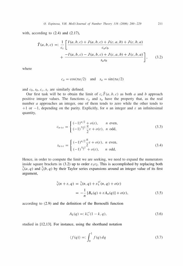
with, according to (2.4) and (2.17),
T̃ (a, b, c) =: 1
cc
[I (a, b, c) + J (a, b, c) + J (c, a, b) + J (c, b, a)
cacb
+ −I (a, b, c) − J (a, b, c) + J (c, a, b) + J (c, b, a)
sasb
], (3.2)
where
ca = cos(�a/2) and sa = sin(�a/2)
and cb, sb, cc, sc are similarly defined.Our first task will be to obtain the limit of ccT̃ (a, b, c) as both a and b approach
positive integer values. The functions ca and sa have the property that, as the realnumber a approaches an integer, one of them tends to zero while the other tends to+1 or −1, depending on the parity. Explicitly, for n an integer and ε an infinitesimalquantity,
cn+ε ={
(−1)n/2 + o(ε), n even,
(−1)n+1
2�
2ε + o(ε), n odd,
(3.3)
sn+ε ={
(−1)n/2 �
2ε + o(ε), n even,
(−1)n−1
2 + o(ε), n odd,(3.4)
Hence, in order to compute the limit we are seeking, we need to expand the numeratorsinside square brackets in (3.2) up to order ε1ε2. This is accomplished by replacing both�̄(a, q) and �̄(b, q) by their Taylor series expansions around an integer value of its firstargument,
�̄(n + ε, q) = �̄(n, q) + ε�̄′(n, q) + o(ε)
= −1
n[Bn(q) + εAn(q)] + o(ε), (3.5)
according to (2.9) and the definition of the Bernoulli function
Ak(q) =: k�′(1 − k, q), (3.6)
studied in [12,13]. For instance, using the shorthand notation
〈f (q)〉 =:∫ 1
0f (q) dq (3.7)

212 O. Espinosa, V.H. Moll / Journal of Number Theory 116 (2006) 200–229
we have
J (c, a, b)| a=n1+ε1b=n2+ε2
= 1
n1n2[〈Bn1(q)Bn2(1 − q)�̄(c, q)〉
+ ε1〈An1(q)Bn2(1 − q)�̄(c, q)〉+ ε2〈Bn1(q)An2(1 − q)�̄(c, q)〉+ ε1ε2〈An1(q)An2(1 − q)�̄(c, q)〉] + o(ε1ε2). (3.8)
Using the reflection property (2.10) of the Bernoulli polynomials and the invariance ofthe integration (3.7) under the change of variable q → 1 − q, we find the followingresult for the numerators inside square brackets in (3.2) (the upper sign corresponds tothe numerator of the first term and the lower sign corresponds to the numerator of thesecond term):
± I (a, b, c) ± J (a, b, c) + J (c, a, b) + J (c, b, a)
= 1
n1n2{±[±1 + (−1)n1 ][±1 + (−1)n2 ]〈Bn1(q)Bn2(q)�̄(c, q)〉
+ε1[±1 + (−1)n2 ]〈An1(q)Bn2(q)�̄+(c, q)〉+ε2[±1 + (−1)n1 ]〈Bn1(q)An2(q)�̄+(c, q)〉+ε1ε2[±〈An1(q)An2(q)�̄+(c, q)〉 + 〈An1(q)An2(1 − q)�̄+(c, q)〉]}+o(ε1ε2), (3.9)
where
�̄+(z, q) := �̄(z, q) + �̄(z, 1 − q). (3.10)
We now examine the behavior of the Tornheim sum as ε1, ε2 → 0. The limitingvalue is obtained from (3.3), (3.4) and (3.9). Observe that T (a, b, c) = T (b, a, c) soonly three cases are presented.
Theorem 3.1. Suppose n1, n2 ∈ N and c ∈ R\N. Then the Tornheim double seriesT (n1, n2, c) are given by
(−1)n1+n2
2(2�)n1+n2
4n1!n2!(2�)c
�(c) cos(�c/2)
[∫ 1
0Bn1(q)Bn2(q)�̄ (c, q) dq − 1
�2
∫ 1
0
×An1(q)An2(q)�̄+(c, q) dq + 1
�2
∫ 1
0An1(q)An2(1 − q)�̄+(c, q) dq
](3.11)

O. Espinosa, V.H. Moll / Journal of Number Theory 116 (2006) 200–229 213
for n1, n2 even;
(−1)n1+n2+1
2(2�)n1+n2
4n1!n2!(2�)c
�(c) cos(�c/2)
[1
�
∫ 1
0Bn1(q)An2(q)�̄+ (c, q) dq
+ 1
�
∫ 1
0An1(q)Bn2(q)�̄+(c, q) dq
](3.12)
for n1 even and n2 odd, and
(−1)n1+n2
2(2�)n1+n2
4n1!n2!(2�)c
�(c) cos(�c/2)
[∫ 1
0Bn1(q)Bn2(q)�̄(c, q) dq − 1
�2
∫ 1
0
×An1(q)An2(q)�̄+(c, q) dq − 1
�2
∫ 1
0An1(q)An2(1 − q)�̄+(c, q) dq
](3.13)
for n1, n2 odd.
The final step in the process is to let c = n3 + ε3 and let ε3 → 0. For n even wesimply have
�̄+(n, q)
cos(�n/2)= −2
n(−1)n/2Bn(q),
whereas for n odd,
limc→n
�̄+(c, q)
cos(�c/2)= −2
n(−1)
n+12
1
�[An(q) + An(1 − q)].
The value of T (n1, n2, n3) is thus expressed in terms of integrals of triple productsof the Bernoulli polynomials Bk(q) = −k�(1 − k, q) and the function Ak(q) = k�′(1 −k, q).
Define the following families of integrals:
R1(n1, n2, n3) =∫ 1
0Bn1(q)Bn2(q)Bn3(q) dq, (3.14)
R2(n1, n2, n3) = 1
�
∫ 1
0Bn1(q)Bn2(q)An3(q) dq, (3.15)
R3(n1, n2, n3) = 1
�2
∫ 1
0An1(q)An2(q)Bn3(q) dq, (3.16)

214 O. Espinosa, V.H. Moll / Journal of Number Theory 116 (2006) 200–229
R4(n1, n2, n3) = 1
�2
∫ 1
0An1(q)An2(1 − q)Bn3(q) dq, (3.17)
R5(n1, n2, n3) = 1
�3
∫ 1
0An1(q)An2(q)An3(q) dq, (3.18)
R6(n1, n2, n3) = 1
�3
∫ 1
0An1(q)An2(q)An3(1 − q) dq. (3.19)
These integrals are all symmetric under interchange of their first two arguments (n1and n2), except for R4 which is antisymmetric if n3 is odd.
Define
p(n) ={
(−1)n/2, n even,
(−1)n+1
2 , n odd.(3.20)
Theorem 3.2. Let � = n1 + n2 + n3. Then the Tornheim double series T (n1, n2, n3) isgiven by
T (n1, n2, n3) = p(�)(2�)�
2n1! n2! n3!TR(n1, n2, n3) (3.21)
where TR(n1, n2, n3) can be expressed in terms of the functions Rj : 1�j �6 as follows:
Case 1: n1, n2 and n3 are even:
TR(n1, n2, n3) = − 12 R1(n1, n2, n3) + R3(n1, n2, n3) − R4(n1, n2, n3). (3.22)
Case 2: n1 and n2 are even; n3 is odd:
TR(n1, n2, n3) = −R2(n1, n2, n3) + R5(n1, n2, n3)
+R6(n1, n2, n3) − R6(n3, n1, n2) − R6(n3, n2, n1). (3.23)
Case 3: n1 is even, n2 is odd, and n3 is even:
TR(n1, n2, n3) = −R2(n3, n1, n2) − R2(n3, n2, n1). (3.24)
Case 4: n1 is even; n2 and n3 are odd:
TR(n1, n2, n3) = R3(n3, n1, n2) + R3(n3, n2, n1)
+R4(n1, n3, n2) + R4(n2, n3, n1). (3.25)
O. Espinosa, V.H. Moll / Journal of Number Theory 116 (2006) 200–229 215
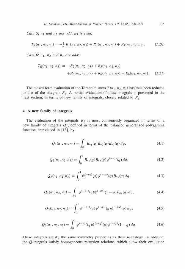
Case 5: n1 and n2 are odd; n3 is even:
TR(n1, n2, n3) = − 12 R1(n1, n2, n3) + R3(n1, n2, n3) + R4(n1, n2, n3). (3.26)
Case 6: n1, n2 and n3 are odd:
TR(n1, n2, n3) = −R2(n1, n2, n3) + R5(n1, n2, n3)
+R6(n1, n2, n3) + R6(n3, n1, n2) + R6(n3, n2, n1). (3.27)
The closed form evaluation of the Tornheim sums T (n1, n2, n3) has thus been reducedto that of the integrals Rj . A partial evaluation of these integrals is presented in thenext section, in terms of new family of integrals, closely related to Rj .
4. A new family of integrals
The evaluation of the integrals Rj is most conveniently organized in terms of anew family of integrals Qj , defined in terms of the balanced generalized polygammafunction, introduced in [13], by
Q1(n1, n2, n3) =∫ 1
0Bn1(q)Bn2(q)Bn3(q) dq, (4.1)
Q2(n1, n2, n3) =∫ 1
0Bn1(q)Bn2(q)�(−n3)(q) dq, (4.2)
Q3(n1, n2, n3) =∫ 1
0�(−n1)(q)�(−n2)(q)Bn3(q) dq, (4.3)
Q4(n1, n2, n3) =∫ 1
0�(−n1)(q)�(−n2)(1 − q)Bn3(q) dq, (4.4)
Q5(n1, n2, n3) =∫ 1
0�(−n1)(q)�(−n2)(q)�(−n3)(q) dq, (4.5)
Q6(n1, n2, n3) =∫ 1
0�(−n1)(q)�(−n2)(q)�(−n3)(1 − q) dq. (4.6)
These integrals satisfy the same symmetry properties as their R-analogs. In addition,the Q-integrals satisfy homogeneous recursion relations, which allow their evaluation
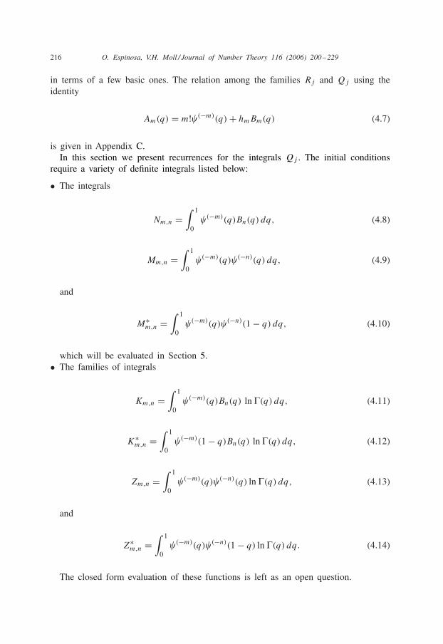
216 O. Espinosa, V.H. Moll / Journal of Number Theory 116 (2006) 200–229
in terms of a few basic ones. The relation among the families Rj and Qj using theidentity
Am(q) = m!�(−m)(q) + hmBm(q) (4.7)
is given in Appendix C.In this section we present recurrences for the integrals Qj . The initial conditions
require a variety of definite integrals listed below:
• The integrals
Nm,n =∫ 1
0�(−m)(q)Bn(q) dq, (4.8)
Mm,n =∫ 1
0�(−m)(q)�(−n)(q) dq, (4.9)
and
M∗m,n =
∫ 1
0�(−m)(q)�(−n)(1 − q) dq, (4.10)
which will be evaluated in Section 5.• The families of integrals
Km,n =∫ 1
0�(−m)(q)Bn(q) ln �(q) dq, (4.11)
K∗m,n =
∫ 1
0�(−m)(1 − q)Bn(q) ln �(q) dq, (4.12)
Zm,n =∫ 1
0�(−m)(q)�(−n)(q) ln �(q) dq, (4.13)
and
Z∗m,n =
∫ 1
0�(−m)(q)�(−n)(1 − q) ln �(q) dq. (4.14)
The closed form evaluation of these functions is left as an open question.
O. Espinosa, V.H. Moll / Journal of Number Theory 116 (2006) 200–229 217
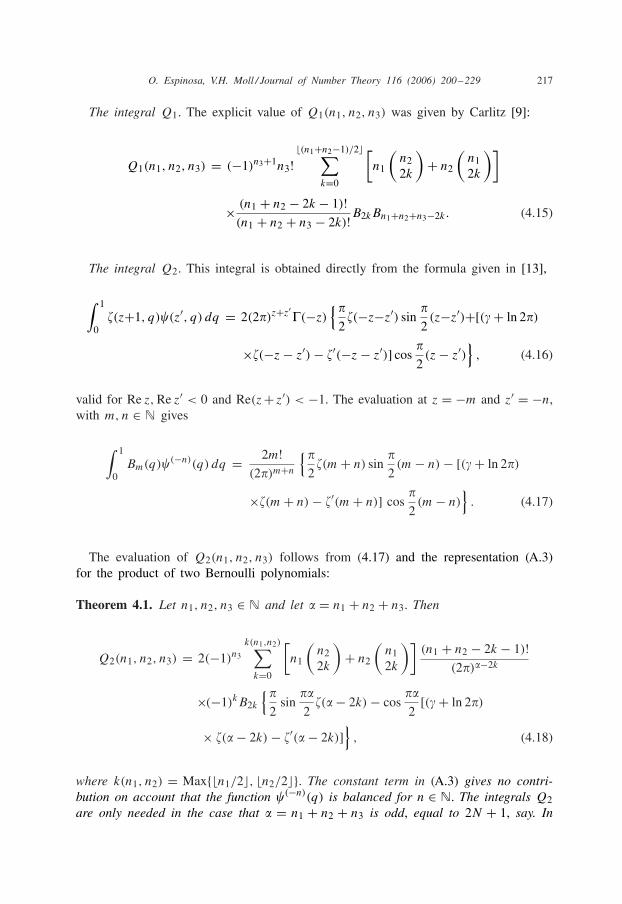
The integral Q1. The explicit value of Q1(n1, n2, n3) was given by Carlitz [9]:
Q1(n1, n2, n3) = (−1)n3+1n3!�(n1+n2−1)/2�∑
k=0
[n1
(n22k
)+ n2
(n12k
)]
× (n1 + n2 − 2k − 1)!(n1 + n2 + n3 − 2k)!B2kBn1+n2+n3−2k. (4.15)
The integral Q2. This integral is obtained directly from the formula given in [13],
∫ 1
0�(z+1, q)�(z′, q) dq = 2(2�)z+z′
�(−z){�
2�(−z−z′) sin
�
2(z−z′)+[(� + ln 2�)
×�(−z − z′) − �′(−z − z′)] cos�
2(z − z′)
}, (4.16)
valid for Re z, Re z′ < 0 and Re(z+ z′) < −1. The evaluation at z = −m and z′ = −n,with m, n ∈ N gives
∫ 1
0Bm(q)�(−n)(q) dq = 2m!
(2�)m+n
{�
2�(m + n) sin
�
2(m − n) − [(� + ln 2�)
×�(m + n) − �′(m + n)] cos�
2(m − n)
}. (4.17)
The evaluation of Q2(n1, n2, n3) follows from (4.17) and the representation (A.3)for the product of two Bernoulli polynomials:
Theorem 4.1. Let n1, n2, n3 ∈ N and let � = n1 + n2 + n3. Then
Q2(n1, n2, n3) = 2(−1)n3
k(n1,n2)∑k=0
[n1
(n22k
)+ n2
(n12k
)](n1 + n2 − 2k − 1)!
(2�)�−2k
×(−1)kB2k
{�
2sin
��
2�(� − 2k) − cos
��
2[(� + ln 2�)
× �(� − 2k) − �′(� − 2k)]}
, (4.18)
where k(n1, n2) = Max{�n1/2�, �n2/2�}. The constant term in (A.3) gives no contri-bution on account that the function �(−n)(q) is balanced for n ∈ N. The integrals Q2are only needed in the case that � = n1 + n2 + n3 is odd, equal to 2N + 1, say. In

218 O. Espinosa, V.H. Moll / Journal of Number Theory 116 (2006) 200–229
this case, sin(��/2) = (−1)N and cos(��/2) = 0, so that
Q2(n1, n2, n3) = �(−1)N+n3 ×k(n1,n2)∑
k=0
[n1
(n22k
)+ n2
(n12k
)]
×(n1 + n2 − 2k − 1)!(2�)�−2k
(−1)kB2k�(� − 2k). (4.19)
Proof. The details are elementary. �
The integral Q3. We now produce a recurrence for
Q3(n1, n2, n3) =∫ 1
0�(−n1)(q)�(−n2)(q)Bn3(q) dq.
The basic tools are the relations
d
dq�(−m)(q) = �(−m+1)(q), (4.20)
and
d
dqBm(q) = mBm−1(q), (4.21)
valid for m ∈ N0, and the fact that both the negapolygamma functions and the Bernoullipolynomials are balanced for the range of indices we wish to consider, i.e., �(−m)(1) =�(−m)(0), for m�2, and Bm(1) = Bm(0), for all m.
Theorem 4.2. Let n1, n2, n3 ∈ N with n1, n2 > 1. Then
(n3 + 1)Q3(n1, n2, n3) = −Q3(n1 − 1, n2, n3 + 1) − Q3(n1, n2 − 1, n3 + 1). (4.22)
Proof. Start with
(n3 + 1)Q3(n1, n2, n3) =∫ 1
0�(−n1)(q) �(−n2)(q)
d
dqBn3+1(q) dq,
integrate by parts and observe that there is no contribution from the boundary. �
The recurrence shows that the value of Q3(n1, n2, n3) can be obtained from thevalues of
Q3(1, m, n) = Km,n + �′(0)Nm,n, (4.23)

O. Espinosa, V.H. Moll / Journal of Number Theory 116 (2006) 200–229 219
in view of �(−1)(q) = ln �(q) + �′(0), the symmetry of the integral Q3 under inter-change of its first two arguments, and the definitions (4.11) and (4.8) of the integralsKm,n, Nm,n.
The integral Q4. Similarly, for n1, n2 > 1, we have that
Q4(n1, n2, n3) =∫ 1
0�(−n1)(q)�(−n2)(1 − q)Bn3(q) dq
satisfies the recurrence
(n3 + 1)Q4(n1, n2, n3) = −Q4(n1 − 1, n2, n3 + 1) + Q4(n1, n2 − 1, n3 + 1), (4.24)
so that it can be obtained from
Q4(1, m, n) = K∗m,n + �′(0)(−1)nNm,n, (4.25)
where K∗m,n is defined in (4.12).
The integrals Q5 and Q6. Similar arguments show that for n1, n2 > 1 we have
Q5(n1, n2, n3) =∫ 1
0�(−n1)(q)�(−n2)(q)�(−n3)(q) dq,
Q6(n1, n2, n3) =∫ 1
0�(−n1)(q)�(−n2)(q)�(−n3)(1 − q) dq,
satisfy the recurrences
Q5(n1, n2, n3) = −Q5(n1 − 1, n2, n3 + 1) − Q5(n1, n2 − 1, n3 + 1) (4.26)
and
Q6(n1, n2, n3) = Q6(n1 − 1, n2, n3 + 1) + Q6(n1, n2 − 1, n3 + 1). (4.27)
The initial conditions are
Q5(1, m, n) = Zm,n + �′(0)Mm,n, (4.28)
Q6(1, m, n) = Z∗m,n + �′(0)M∗
m,n, (4.29)
where Zm,n, Z∗m,n, Mm,n and M∗
m,n are defined in (4.13), (4.14), (4.9) and (4.10),respectively.

220 O. Espinosa, V.H. Moll / Journal of Number Theory 116 (2006) 200–229
5. Evaluation of integrals
5.1. The product of a Bernoulli polynomial and a balanced negapolygamma
The explicit evaluation of the integral Nm,n defined by (4.8) was obtained in (4.17)as a byproduct of the evaluation of Q2:
Nm,n = 2n!(2�)m+n
{�
2�(m + n) sin
�
2(n − m)
−[(� + ln 2�)�(m + n) − �′(m + n)] cos�
2(n − m)
}. (5.1)
5.2. The product of two balanced negapolygammas
The integral of the product of two balanced negapolygamma functions has been givenin [12]:
Let k, k′ ∈ N, k+ = k + k′ and k− = k − k′. Then
Mk,k′ =∫ 1
0�(−k)(q)�(−k′)(q) dq
= 2
(2�)k+ cos(�
2k−
)[A+�(k+) − 2A�′(k+) + �′′(k+)], (5.2)
where A = � + ln 2� and A± = A2 ± �2/4.Similarly, one finds
M∗k,k′ =
∫ 1
0�(−k)(q)�(−k′)(1 − q) dq
= 2
(2�)k+
{cos
(�
2k+
)[A−�(k+) − 2A�′(k+) + �′′(k+)]
+� sin(�
2k+
)[A�(k+) − �′(k+)]
}. (5.3)
We have been unable to obtain closed form results for the integrals Km,n K∗m,n, Zm,n
and Z∗m,n, which involve the kernel ln �(q) and one or two negapolygamma functions.
6. Some examples
In this section we describe some explicit evaluations of Tornheim sums. It is conve-nient to introduce the function
Um,n =∫ 1
0�(−m)(q)Bn(q) ln sin(�q) dq. (6.1)

O. Espinosa, V.H. Moll / Journal of Number Theory 116 (2006) 200–229 221
The identity
ln �(q) + ln �(1 − q) = ln � − ln sin(�q) (6.2)
yields the relation
Km,n + (−1)nK∗m,n = ln �Nm,n − Um,n. (6.3)
Example 6.1. We consider the value of T (1, 1, 2). This corresponds to Case 5 ofTheorem 3.2. It yields
T (1, 1, 2) = 4�4[−1
2R1(1, 1, 2) + R3(1, 1, 2) + R4(1, 1, 2)
], (6.4)
and in terms of the Qj -family,
T (1, 1, 2) = 4�4[−1
2Q1(1, 1, 2) + 1
�2 Q3(1, 1, 2) + 1
�2 Q4(1, 1, 2)
]. (6.5)
The Qj -integrals are given by
Q1(1, 1, 2) = 1
180,
Q3(1, 1, 2) = K1,2 + �′(0)N1,2,
Q4(1, 1, 2) = K∗1,2 + �′(0)N1,2
and using the values �′(0) = − 12 ln(2�) and N1,2 = �(3)/4�2 we obtain
T (1, 1, 2) = 4�2(K1,2 + K∗1,2) − �(3) ln(2�) − 1
90�4.
In terms of the U-function this can be written as
T (1, 1, 2) = −4�2U1,2 − �(3) ln 2 − 1
90�4. (6.6)
The identities (1.16) and (1.17) yield T (1, 1, 2) = 2T (0, 1, 3), and the method ofHuard et al. [17] yields the values of T (n1, n2, n3) for N = n1+n2+n3 odd and also forN = 4 and 6. For instance T (0, 1, 3) = 1
4�(4). This yields an evaluation of an integral

222 O. Espinosa, V.H. Moll / Journal of Number Theory 116 (2006) 200–229
of type Um,n: the value T (1, 1, 2) = �(4)/2, the identity �(−1)(q) = ln �(q) + �′(0)
and
∫ 1
0B2(q) ln(sin �q) dq = −�(3)
2�2
given in Example 5.2 of [11] produce
∫ 1
0B2(q) ln �(q) ln(sin �q) dq = −
(�2
240+ ln(4�) �(3)
4�2
). (6.7)
It follows that
U1,2 = − �2
240− ln 2 �(3)
4�2 . (6.8)
Example 6.2. The explicit expression for R2(n1, n2, n3) that can be obtained from(C.2) through (4.15) and (4.18) permits the evaluation of T (n1, n2, n3) in the casen1, n3 even and n2 odd. For example
T (2, 1, 2) = �2
6�(3) − 3
2�(5),
T (2, 3, 2) = −�2
6�(5) + 2�(7),
and
T (4, 3, 2) = �4
90�(5) + �2
6�(7) − 5
2�(9).
Example 6.3. Define w = a+b+c to be the weight of the sum T (a, b, c). The resultsof the procedure described above for sums of small weight are given below.Weight 3:
T (1, 1, 1) = 4Z1,1 + 12Z∗1,1 − �(3) + ln 2�
(A2
3− �2
6− 4A�′(2)
�2 + 2�′′(2)
�2
),
Weight 4:
T (1, 1, 2) = −4�2U1,2 − �4
90− �(3) ln 2,
T (1, 2, 1) = −4�2(U1,2 + 2U2,1),

O. Espinosa, V.H. Moll / Journal of Number Theory 116 (2006) 200–229 223
Weight 5:
T (1, 1, 3) = −8�2(K∗1,3 + 2Z1,3 + 2Z∗
1,3 + 4Z∗3,1) − �(5)
+ ln 2�
(�2A2
45− �2A
30− �4
90− 4�′ (4) A
�2 + 3�′ (4)
�2 + 2�′′ (4)
�2
),
T (1, 2, 2) = �2
6�(3) − 3
2�(5),
T (1, 3, 1) = −8�2(K∗1,3 + 2Z3,1 + 2Z∗
1,3 + 4Z∗3,1) + �2
6�(3) − 2�(5)
+ ln 2�
(�2A2
45− �2A
30− �4
90− 4�′(4)A
�2 + 3�′(4)
�2 + 2�′′(4)
�2
),
T (2, 2, 1) = 32�2Z2,2 + �2
3�(3) − 3�(5)
+ ln 2�
(−�2A2
45− �4
180+ 4�′(4)A
�2 − 2�′′(4)
�2
).
We have produced some partial results in the evaluation of the integrals Km,n, K∗m,n
and Zm,n, Z∗m,n. These suggest that the value of the Tornheim sums can be expressed
in terms of a small number of definite integrals. For instance, for m�3 odd, we havethe relation
Km,n = −mKm−1,n+1 + ln√
2�(Nm,n + mNm−1,n+1)
−∫ 1
0Bm(q)�(q)�(−n−1)(q) dq,
which reduces the value of Km,n to that of K1,m+n−1 plus the moments of the product�(q)�(−j)(q). Details will be presented elsewhere.
Acknowledgments
The first author would like to thank the Department of Mathematics at Tulane Uni-versity for its hospitality, and the partial support of grant MECESUP FSM0204. Thesecond author acknowledges the partial support of NSF-DMS 0070567.
224 O. Espinosa, V.H. Moll / Journal of Number Theory 116 (2006) 200–229
Appendix A. The Bernoulli polynomials
The Bernoulli polynomials Bn(q) defined by the generating function
xexq
ex − 1=
∞∑n=0
Bn(q)xn
n! . (A.1)
The Bernoulli numbers Bn = Bn(0) satisfy
Bn(q) =n∑
k=0
(n
k
)Bkq
n−k. (A.2)
For n�1 we have the differential recursion B ′n(q) = nBn−1(q) and the symmetry rule
Bn(1 − q) = (−1)nBn(q). In particular, Bn(1) = Bn(0) for n > 1.The Bernoulli polynomials {B0(q), B1(q), . . . , Bn(q)} form a basis for the space of
polynomials of degree at most n. Thus the product Bn1(q)Bn2(q) is a linear combinationof Bj (q) for j = 0, . . . , n1 + n2. It is a remarkable fact that this combination has theexplicit form
Bn1(q)Bn2(q) =k(n1,n2)∑
k=0
[n1
(n22k
)+ n2
(n12k
)]B2k
n1 + n2 − 2kBn1+n2−2k(q)
+(−1)n1+1 n1! n2!(n1 + n2)!Bn1+n2 , (A.3)
where k(n1, n2) = Max{�n1/2�, �n2/2�}. In terms of rescaled Bernoulli polynomialsand numbers, defined by
B̃n(q) = Bn(q)
n! , B̃n = B̃n(0) = Bn
n! , (A.4)
relation (A.3) has the simpler form
B̃n1(q)B̃n2(q) =k(n1,n2)∑
k=0
[(n1 + n2 − 2k − 1
n1 − 1
)+
(n1 + n2 − 2k − 1
n2 − 1
)]
×B̃2kB̃n1+n2−2k(q) + (−1)n1+1B̃n1+n2 . (A.5)
In theory, (A.3) yields expressions for a product of any number of Bernoulli poly-nomials. For example,
B2n(q) =
�n/2�∑k=0
n(
n2k
)n − k
B2kB2n−2k(q) + (−1)n+1 B2n(2nn
) , (A.6)

O. Espinosa, V.H. Moll / Journal of Number Theory 116 (2006) 200–229 225
or
B̃2n(q) = 2
�n/2�∑k=0
(2n − 2k − 1
n − 1
)B̃2kB̃2n−2k(q) + (−1)n+1B̃2n, (A.7)
and
B3n(q) =
�n/2�∑k=0
n(
n2k
)n − k
B2k
n−k∑j=0
[n
(2n − 2k
2j
)+ 2(n − k)
(n
2j
)]B2j B3n−2k−2j (q)
3n − 2k − 2j
+(−1)n+1
⎡⎣ B2n(
2nn
)Bn(q) + 2n!3�n/2�∑k=0
(2n − 2k − 1
n − 1
)B2kB3n−2k
(2k)!(3n − 2k)!
⎤⎦ .
(A.8)
or
B̃3n(q) = 2
�n/2�∑k=0
(2n − 2k − 1
n − 1
)B̃2k
n−k∑j=0
[(3n − 2k − 2j − 1
n − 1
)
+(
3n − 2k − 2j − 12n − 2k − 1
)]B̃2j B̃3n−2k−2j (q)
+(−1)n+1
⎡⎣B̃2nB̃n(q) + 2
�n/2�∑k=0
(2n − 2k − 1
n − 1
)B̃2kB̃3n−2k
⎤⎦ . (A.9)
Integrating the relation (A.1) yields
∫ 1
0Bn(q) dq = 0, for n�1. (A.10)
Apostol [3] gives a direct proof of
∫ 1
0Bn1(q)Bn2(q) dq = (−1)n1+1 n1! n2!
(n1 + n2)!Bn1+n2 , (A.11)
for n1, n2 ∈ N.The Bernoulli polynomials appear also as special values of the Hurwitz zeta function
�(1 − k, q) = −1
kBk(q). (A.12)

226 O. Espinosa, V.H. Moll / Journal of Number Theory 116 (2006) 200–229
Appendix B. The generalized polygamma function �(z, q)
The polygamma function is defined by
�(m)(q) = dm
dqm�(q), m ∈ N, (B.1)
where
�(q) = �(0)(q) = d
dqln �(q) (B.2)
is the digamma function.The function �(m) is analytic in the complex q-plane, except for poles (of order
m+ 1) at all non-positive integers. Extensions of this function for m a negative integerhave been defined by several authors [1,12,15]. These are the negapolygamma functions.For example, Gosper [15] defined
�−1(q) = ln �(q),
�−k(q) =∫ q
0�−k+1(t) dt, k�2, (B.3)
which were later reconsidered by Adamchik [1] in the form
�−k(q) = 1
(k − 2)!∫ q
0(q − t)k−2 ln �(t) dt, k�2. (B.4)
These extensions can be expressed in terms of the derivative (with respect to its firstargument) of the Hurwitz zeta function at the negative integers [1,15]. The definition(B.3) can be modified by introducing arbitrary constants of integration at every step.This yields different extensions differing by polynomials:
�(−m)a (q) − �(−m)
b (q) = pm−1(q),
satisfying
pn(q) = d
dqpn+1(q).
A new extension of �(m)(q) has been introduced in [12], in connection with inte-grals involving the polygamma and the loggamma functions. These are the balancednegapolygamma functions, defined for m ∈ N by
�(−m)(q) := 1
m! [Am(q) − Hm−1Bm(q)]. (B.5)

O. Espinosa, V.H. Moll / Journal of Number Theory 116 (2006) 200–229 227
Here Hr = 1 + 1/2 + . . . + 1/r is the harmonic number (H0 = 0), Bm(q) is the mthBernoulli polynomial, and
Am(q) = m �′(1 − m, q). (B.6)
A function f (q) is defined on (0, 1) is called balanced if its integral over (0, 1) vanishesand f (0) = f (1). In [12] we have shown that
d
dq�(−m)(q) = �(−m+1)(q), m ∈ N. (B.7)
The function �(z, q) defined in (1.15) represents an extension of these polygammafamilies to q ∈ C. Its main properties are presented in the next theorem. The detailsappear in [13].
Theorem B.1. The generalized polygamma function �(z, q) satisfies:
• For fixed q ∈ C, the function �(z, q) is an entire function of z.• For m ∈ Z : �(m, q) = �(m)(q).• It satisfies
��q
�(z, q) = �(z + 1, q). (B.8)
Appendix C. The relation between Qj and Rj
Using the relation (4.7) we can express the integrals Rj , defined by (3.14)–(3.19)in terms of Qj , defined by (4.1)–(4.6). Recall that, for n > 1 we have hn = 1 + 1/2+ · · · + 1/(n − 1) and h1 = 0.
R1(n1, n2, n3) = Q1(n1, n2, n3), (C.1)
�R2(n1, n2, n3) = n3!Q2(n1, n2, n3) + hn3Q1(n1, n2, n3), (C.2)
�2R3(n1, n2, n3) = n1!n2!Q3(n1, n2, n3) + n2!hn1Q2(n1, n3, n2)
+n1!hn2Q2(n2, n3, n1) + hn1hn2Q1(n1, n2, n3), (C.3)
�2R4(n1, n2, n3) = n1!n2!Q4(n1, n2, n3) + (−1)n2n1!hn2Q2(n2, n3, n1)
+(−1)n1+n3n2!hn1Q2(n1, n3, n2)
+(−1)n2hn1hn2Q1(n1, n2, n3), (C.4)

228 O. Espinosa, V.H. Moll / Journal of Number Theory 116 (2006) 200–229
�3R5(n1, n2, n3) = n1!n2!n3!Q5(n1, n2, n3) + n1!n2!hn3Q3(n1, n2, n3)
+n1!n3!hn2Q3(n1, n3, n2) + n2!n3!hn1Q3(n2, n3, n1)
+n1!hn2hn3Q2(n2, n3, n1) + n2!hn1hn3Q2(n1, n3, n2)
+n3!hn1hn2Q2(n1, n2, n3) + hn1hn2hn3Q1(n1, n2, n3), (C.5)
�3R6(n1, n2, n3) = n1!n2!n3!Q6(n1, n2, n3) + (−1)n3n1!n2!hn3Q3(n1, n2, n3)
+n1!n3!hn2Q4(n1, n3, n2) + n2!n3!hn1Q4(n2, n3, n1)
+(−1)n3n1!hn2hn3Q2(n2, n3, n1)
+(−1)n3n2!hn1hn3Q2(n1, n3, n2)
+(−1)n1+n2n3!hn1hn2Q2(n1, n2, n3)
+(−1)n3hn1hn2hn3Q1(n1, n2, n3). (C.6)
References
[1] V. Adamchik, Polygamma functions of negative order, J. Comput. Appl. Math. 100 (1998) 191–198.[2] V. Adamchik, Multiple Gamma function and its application to computation of series, Ramanujan J.
9 (2005) 271–288.[3] T. Apostol, Introduction to Analytic Number Theory, UTM, Springer, Berlin, 1976.[4] B. Berndt, On the Hurwitz zeta function, Rocky Mountain J. 2 (1972) 151–157.[5] G. Boros, O. Espinosa, V. Moll, On some families of integrals solvable in terms of polygamma and
negapolygamma functions, Integral Transforms Special Funct. 14 (3) (2003) 187–203.[6] J. Borwein, D. Bailey, R. Girgensohn, Experimentation in Mathematics: Computational Paths to
Discovery, A.K. Peters, 2004.[7] K.N. Boyadzhiev, Evaluation of Euler–Zagier sums, Internat. J. Math. Sci. 27 (2001) 407–412.[8] K.N. Boyadzhiev, Consecutive evaluation of Euler sums, Internat. J. Math. Sci. 29 (2002) 555–561.[9] L. Carlitz, Note on the integral of the product of several Bernoulli polynomials, J. London Math.
Soc. 34 (1959) 361–363.[10] R. Crandall, J. Buhler, On the evaluation of Euler sums, Exp. Math. 3 (1994) 275–285.[11] O. Espinosa, V. Moll, On some integrals involving the Hurwitz zeta function: part 1, Ramanujan J.
6 (2002) 159–188.[12] O. Espinosa, V. Moll, On some integrals involving the Hurwitz zeta function: part 2, Ramanujan J.
6 (2002) 449–468.[13] O. Espinosa, V. Moll, A generalized polygamma function, Integral Transforms Special Funct. 15
(2004) 101–115.[14] O. Espinosa, V. Moll, The evaluation of Tornheim double sums, Part 2, in preparation.
[15] R.Wm. Gosper Jr,∫ m/6n/4 ln �(z) dz. In Special functions. q-series and related topics, in: M. Ismail,
D. Masson, M. Rahman (Eds.), The Fields Institute Communications, AMS, Providence, RI, 1997,pp. 71–76.

O. Espinosa, V.H. Moll / Journal of Number Theory 116 (2006) 200–229 229
[17] J.G. Huard, K.S. Williams, N.Y. Zhang, On Tornheim’s double series, Acta Arith. 75 (1996) 105–117.
[18] D. Kreimer, Knots and Feynman diagrams, Cambridge Lecture Notes in Physics, 2000.[19] K. Matsumoto, On the analytic continuation of various multiple zeta-functions, in: M.A. Bennett
et al. (Eds.), Number Theory for the Millenium II, Proceedings of the Millenium Conference onNumber Theory, A.K. Peters, 2002, pp. 417–440.
[23] R. Sitaramachandrarao, M.V. Subbarao, Transformation formulae for multiple series, Pacific J. Math.113 (1984) 471–479.
[25] L. Tornheim, Harmonic double series, Amer. J. Math. 72 (1950) 303–314.[27] H. Tsumura, On Witten’s type zeta values attached to SO(5), Arch. Math. 82 (2004) 145–152.[30] E. Whittaker, G. Watson, A Course of Modern Analysis, fourth ed., reprinted, Cambridge University
Press, Cambridge, MA, 1963.[32] D. Zagier, Values of zeta functions and their applications, First European Congress of Mathematics,
vol. 2, Paris, 6–10 July, 1992, Birkhauser Verlag, Basel, pp. 497–512.
Further reading
[16] M. Hoffman, Multiple harmonic series, Pacific J. Math. 152 (1992) 275–290.[20] K. Matsumoto, On Mordell–Tornheim and other multiple zeta functions, in: D.R. Heath-Brown, B.Z.
Moroz (Eds.), Proceedings of the Session in Analytic Number Theory and Diophantine Equations,Bonn, January–June 2002, Bonner Mathematische Schriften, Nr. 360, Bonn, 2003, n. 25, 17pp.
[21] L.J. Mordell, On the evaluation of some multiple series, J. London Math. Soc. 33 (1958) 368–371.[22] L.J. Mordell, Integral formulae of arithmetical character, J. London Math. Soc. 33 (1958) 371–375.[24] M.V. Subbarao, R. Sitaramachandrarao, On some infinite series of L.J. Mordell and their analogues,
Pacific J. Math. 113 (1985) 245–255.[26] H. Tsumura, On some combinatorial relations for Tornheim’s double series, Acta Arith. 105 (3)
(2002) 239–252.[28] H. Tsumura, On a class of combinatorial relations for Tornheim’s type of triple series, preprint.[29] H. Tsumura, On Mordell–Tornheim zeta values, Proceedings of the American Mathematical Society
133 (2005) 2387–2393.[31] E. Witten, On quantum gauge theories in two dimensions, Comm. Math. Phys. 141 (1991) 153–209.