Proc. of the 15th Int. Conference on Digital Audio Effects (DAFx-12), York, UK , September 17-21, 2012

THE HELMHOLTZ RESONATOR TREE

Rafael C. D. Paiva and Vesa Välimäki∗

Department of Signal Processing and AcousticsAalto University, School of Electrical Engineering

Espoo, Finlandrafael.dias.de.paiva@aalto.fi vesa.valimaki@aalto.fi

ABSTRACT

The Helmholtz resonator is a prototype of a single acoustic res-onance, which can be modeled with a digital resonator. This pa-per extends this concept by coupling several Helmholtz resonators.The resulting structure is called a Helmholtz resonator tree. Theheight of the tree is defined by the number of resonator layersthat are interconnected. The overall number of resonance frequen-cies of a Helmholtz resonator tree is the same as its height. AHelmholtz resonator tree can be modeled using wave digital filters(WDF), when electro-acoustic analogies are applied. A WDF toolfor implementing Helmholtz resonator trees has been developed inC++. A VST plugin and an Android mobile application were cre-ated, which can run short Helmholtz resonator trees in real time.Helmholtz resonator trees can be used for the real-time synthesisof percussive sounds and for realizing novel filtering which can betuned using intuitive physical parameters.

1. INTRODUCTION

Musical acoustics have many applications in understanding musi-cal instruments and building computational tools. These computa-tional tools may be used to create new digital musical instrumentsas well as to build digital effects based on intuitive physical phe-nomena. Some interesting phenomena derive from Helmholtz res-onances [1]. These resonances are related to the body of acousticstring instruments, such as the guitar or violin, wind instruments,such as the flute or a simple ocarina, and the cavity of percussioninstruments, such as the hang [2].

The physical description of musical phenomena use a varietyof techniques [3]. Digital waveguides are used to model vibrat-ing phenomena like strings and airflow in wind instruments [4].The mass-spring models are used to create vibrating structures inan intuitive way [5, 3]. The modes of a system may be repre-sented using coupled mode synthesis [6], modal synthesis [7], orthe functional transformation method [8]. Various percussive mu-sical instruments have been successfully modeled using a digitalwaveguide mesh [9, 10, 11], modal synthesis [12], and finite dif-ferences [13]. Additionally, there are a variety of models of elec-tric circuits. These include state-space methods [14, 15], the Kmethod [16] and wave digital filters (WDF) [17, 18] among oth-ers. WDF applications include the model of a piano hammer [19],models of vacuum tube amplifiers [20], and a model of an audiotransformer in vacuum tube amplifiers [21].

This paper proposes the combination of several Helmholtz reso-nators in a tree-like structure, which is called a Helmholtz resona-tor tree. Such structures can be modeled using WDFs when elec-

∗ This work was supported by the Nokia Foundation.

tro-acoustic analogies are applied. This leads to real-time physicalmodeling of complex resonant structures, where the input and out-put points can be located at any of the interconnected resonators.

The Helmholtz resonator tree yields an intuitive way of creat-ing physically-inspired resonating structures for synthesis. In thistype of structure several resonators influence each other, and theirparameters can be modified using acoustical parameters, which areintuitive even for non-technical people, although the exact res-onance frequencies are unknown. Additionally, it provides thepossibility of exciting the system at different points, resulting intimbre variations of the same musical instrument. This approachdiffers from the implementation of cascaded second order filters,since the resonators interact with each other, changing their reso-nance frequencies.

This paper is organized as follows. Section 2 presents a re-view of the acoustic-electric analogy for obtaining an equivalentmodel a Helmholtz resonator and extending it to a Helmholtz res-onator tree structure. Section 3 reviews basic WDF concepts. Sec-tion 4 introduces the Helmholtz resonator tree tool with a VSTplugin and an Android mobile application as implementation ex-amples. Section 5 shows simulation results to evaluate the effectof the Helmholtz resonator tree structure and compares the compu-tational cost of the implemented system with a commercial circuitsimulator software. Section 6 concludes the paper.

2. HELMHOLTZ RESONATOR

2.1. Basic concept

The Helmholtz resonator, which is a prototype of a simple acous-tic resonant system, can be thought to be a hollow shell, like abottle, enclosing a volume connected to the external environmentthrough an open pipe, or neck, as shown in Fig. 1(a). This struc-ture is specified by the cavity volume V0, the neck length l, theneck cross-sectional area S, and parameters of the surrounding en-vironment [22], namely the speed of sound c and the density ρ ofthe surrounding gas where the resonator is located. These param-eters are typically c = 345 m/s and ρ = 1.2 kg/m3 at roomtemperature.

In order to derive the Helmholtz resonator model, the impe-dance of each acoustic part needs to be determined. The generalimpedance of an acoustic system is given by

Z =p

U=

p

Su, (1)

where p is the gas pressure, U is the volume velocity, u the par-ticle velocity, and S the cross sectional area. By using the anal-ogy pressure→voltage and volume flow→current, it is possible to

DAFX-1

Proc. of the 15th Int. Conference on Digital Audio Effects (DAFx-12), York, UK , September 17-21, 2012

V0, p0

l

SU1, p1

U1

p1 p0C

R L

(a) (b)

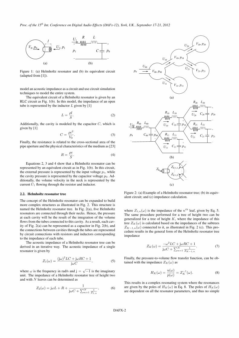
Figure 1: (a) Helmholtz resonator and (b) its equivalent circuit(adapted from [1]).

model an acoustic impedance as a circuit and use circuit simulationtechniques to model the entire system.

The equivalent circuit of a Helmholtz resonator is given by anRLC circuit as Fig. 1(b). In this model, the impedance of an opentube is represented by the inductor L given by [1]

L =ρl

S. (2)

Additionally, the cavity is modeled by the capacitor C, which isgiven by [1]

C =ρc2

V0. (3)

Finally, the resistance is related to the cross-sectional area of thepipe aperture and the physical characteristics of the medium as [23]

R =ρc

S. (4)

Equations 2, 3 and 4 show that a Helmholtz resonator can berepresented by an equivalent circuit as in Fig. 1(b). In this circuit,the external pressure is represented by the input voltage p1, whilethe cavity pressure is represented by the capacitor voltage p0. Ad-ditionally, the volume velocity in the neck is represented by thecurrent U1 flowing through the resistor and inductor.

2.2. Helmholtz resonator tree

The concept of the Helmholtz resonator can be expanded to buildmore complex structures as illustrated in Fig. 2. This structure isnamed the Helmholtz resonator tree. In Fig. 2(a), five Helmholtzresonators are connected through their necks. Hence, the pressureat each cavity will be the result of the integration of the volumeflows from the tubes connected to this cavity. As a result, each cav-ity of Fig. 2(a) can be represented as a capacitor in Fig. 2(b), andthe connections between cavities through the tubes are representedby circuit connections with resistors and inductors correspondingto the impedance of each tube.

The acoustic impedance of a Helmholtz resonator tree can bederived in an iterative way. The acoustic impedance of a singleresonator is given by

Z1(ω) =(jω)2LC + jωRC + 1

jωC, (5)

where ω is the frequency in rad/s and j =√−1 is the imaginary

unit. The impedance of a Helmholtz resonator tree of height twoand with N leaves can be determined as

Z2(ω) = jωL+R+1

jωC +∑N

n=11

Z1,n

, (6)

V00, p00

V10, p10

V11, p11

V20, p20

V21, p21 p0

U10

U20

U11

U21U00

(a)

U00

p0 p00C00

L00R00

p20

p21

L10R10

L11R11

L20R20

L21R21p10C10

p11C11

C20

C21

U10

U11

U21

U20

(b)

ZKZK-1,1

ZK-1,N

(c)

Figure 2: (a) Example of a Helmholtz resonator tree; (b) its equiv-alent circuit; and (c) impedance calculation.

where Z1,n(ω) is the impedance of the nth leaf, given by Eq. 5.The same procedure performed for a tree of height two can begeneralized for a tree of height K, where the impedance of thistree ZK(ω) is calculated based on the impedances of the subtreesZK−1,n(ω) connected to it, as illustrated in Fig. 2 (c). This pro-cedure results in the general form of the Helmholtz resonator treeimpedance

ZK(ω) =−ω2LC + jωRC + 1

jωC +∑N

n=11

ZK−1,n

. (7)

Finally, the pressure-to-volume flow transfer function, can be ob-tained with the impedance ZK(ω) as

HK(ω) =u(ω)

p(ω)= Z−1

K (ω). (8)

This results in a complex resonating system where the resonancesare given by the poles of HK(ω) in Eq. 8. The poles of HK(ω)are dependent on all the resonator parameters, and thus no simple

DAFX-2

Proc. of the 15th Int. Conference on Digital Audio Effects (DAFx-12), York, UK , September 17-21, 2012

closed-formula solution can be found for the resonating frequen-cies of this type of system. A demonstrative video illustrates the ef-fect of changing a single resonator at http://www.acoustics.hut.fi/go/dafx12-helmholtztree.

2.3. Helmholtz resonator tree structure effect

The parameters of the Helmholtz resonator tree were evaluatedwith Eq. 8 in two sets of results. In the first, the effect of the treeheight and number of branch divisions is evaluated, while in thesecond set the effect of individual physical resonator parameters isevaluated.

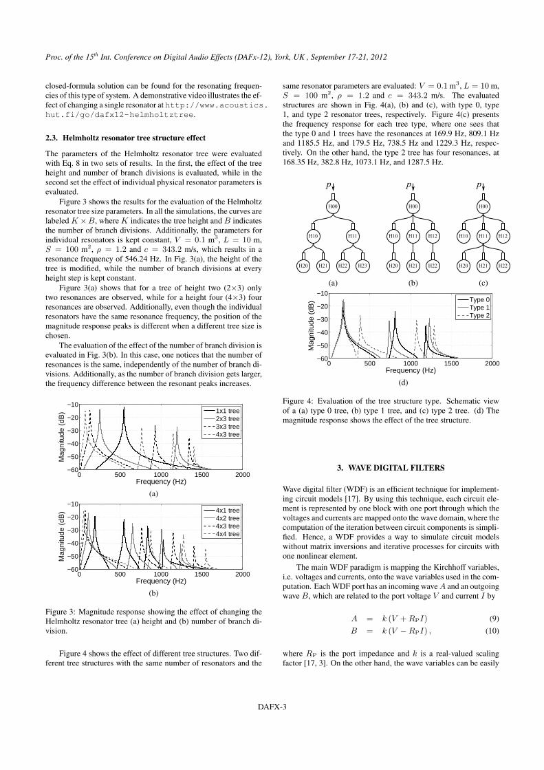
Figure 3 shows the results for the evaluation of the Helmholtzresonator tree size parameters. In all the simulations, the curves arelabeled K ×B, where K indicates the tree height and B indicatesthe number of branch divisions. Additionally, the parameters forindividual resonators is kept constant, V = 0.1 m3, L = 10 m,S = 100 m2, ρ = 1.2 and c = 343.2 m/s, which results in aresonance frequency of 546.24 Hz. In Fig. 3(a), the height of thetree is modified, while the number of branch divisions at everyheight step is kept constant.

Figure 3(a) shows that for a tree of height two (2×3) onlytwo resonances are observed, while for a height four (4×3) fourresonances are observed. Additionally, even though the individualresonators have the same resonance frequency, the position of themagnitude response peaks is different when a different tree size ischosen.

The evaluation of the effect of the number of branch division isevaluated in Fig. 3(b). In this case, one notices that the number ofresonances is the same, independently of the number of branch di-visions. Additionally, as the number of branch division gets larger,the frequency difference between the resonant peaks increases.

0 500 1000 1500 2000−60

−50

−40

−30

−20

−10

Frequency (Hz)

Mag

nitu

de (

dB)

1x1 tree2x3 tree3x3 tree4x3 tree

(a)

0 500 1000 1500 2000−60

−50

−40

−30

−20

−10

Frequency (Hz)

Mag

nitu

de (

dB)

4x1 tree4x2 tree4x3 tree4x4 tree

(b)

Figure 3: Magnitude response showing the effect of changing theHelmholtz resonator tree (a) height and (b) number of branch di-vision.

Figure 4 shows the effect of different tree structures. Two dif-ferent tree structures with the same number of resonators and the

same resonator parameters are evaluated: V = 0.1 m3, L = 10 m,S = 100 m2, ρ = 1.2 and c = 343.2 m/s. The evaluatedstructures are shown in Fig. 4(a), (b) and (c), with type 0, type1, and type 2 resonator trees, respectively. Figure 4(c) presentsthe frequency response for each tree type, where one sees thatthe type 0 and 1 trees have the resonances at 169.9 Hz, 809.1 Hzand 1185.5 Hz, and 179.5 Hz, 738.5 Hz and 1229.3 Hz, respec-tively. On the other hand, the type 2 tree has four resonances, at168.35 Hz, 382.8 Hz, 1073.1 Hz, and 1287.5 Hz.

H20 H21 H22 H23

H10 H11

p

H00

H10 H12

p

H00

H11

H20 H22H21

H10 H12

p

H00

H11

H20 H22H21

(a) (b) (c)

0 500 1000 1500 2000−60

−50

−40

−30

−20

−10

Frequency (Hz)

Mag

nitu

de (

dB)

Type 0Type 1Type 2

(d)

Figure 4: Evaluation of the tree structure type. Schematic viewof a (a) type 0 tree, (b) type 1 tree, and (c) type 2 tree. (d) Themagnitude response shows the effect of the tree structure.

3. WAVE DIGITAL FILTERS

Wave digital filter (WDF) is an efficient technique for implement-ing circuit models [17]. By using this technique, each circuit ele-ment is represented by one block with one port through which thevoltages and currents are mapped onto the wave domain, where thecomputation of the iteration between circuit components is simpli-fied. Hence, a WDF provides a way to simulate circuit modelswithout matrix inversions and iterative processes for circuits withone nonlinear element.

The main WDF paradigm is mapping the Kirchhoff variables,i.e. voltages and currents, onto the wave variables used in the com-putation. Each WDF port has an incoming waveA and an outgoingwave B, which are related to the port voltage V and current I by

A = k (V +RPI) (9)B = k (V −RPI) , (10)

where RP is the port impedance and k is a real-valued scalingfactor [17, 3]. On the other hand, the wave variables can be easily

DAFX-3

Proc. of the 15th Int. Conference on Digital Audio Effects (DAFx-12), York, UK , September 17-21, 2012

converted again into Kirchhoff variables as

V =A+B

2k(11)

I =A−B2kRP

. (12)

It is important to notice that the port impedance RP is not neces-sarily related to the impedance of the element being simulated. Inmost of the cases,RP is adjusted in order to provide reflection-freeelements, but this is not necessarily mandatory for all elements.

Reflection-free ports constitute an important issue in WDF.Elements using reflection-free ports are also called adapted ele-ments. When this kind of port is used, the output wave of an el-ement has no instantaneous dependency on the incoming wave.This means that the computation of the outgoing wave for that ele-ment will imply in no recursive method for the computation of thecircuit response. Typically, multiport elements can only have onereflection-free port. One example of how this is represented in thedrawings of this work is presented in Fig. 5(a), where a generictree-port element X is connected to other elements through portswith impedance Rp0, Rp1 and Rp2. In this representation, thedash at the beginning of the line representing the port connectionRp0 indicates that this port is adapted.

X

Rp1 Rp2

Rp0

(a)

(b) (c)

Figure 5: Drawing nomenclature used in this paper. (a) A genericmulti-port element with one reflection-free port and tree port (b)series and (c) parallel adaptors with one reflection-free port.

4. HELMHOLTZ RESONATOR TREE TOOL

In order to encapsulate the behavior of Helmholtz resonators, aC++ tool for simulating these resonators was implemented. Thistool is built using WDF classes to simulate circuit elements anduses its own classes for generating Helmholtz resonator tree struc-tures and managing the connections between resonators.

Figure 6 shows the basic elements of a Helmholtz resonatorimplemented in the C++ tool. The acoustic representation of ageneric Helmholtz resonator is presented in Fig. 6(a), which maybe connected to the cavity of another resonator through its neck,

and it may be connected to several other resonators in its cav-ity. In this system, each resonator can be excited with an exter-nal source of volume flow U0, which simulates something hittingthat resonator. The equivalent circuit of the resonator is shown inFig. 6(b), which includes a capacitor simulating the resonator cav-ity, the neck model with a resistor and an inductor, and a currentsource simulates the volume flow disturbance at the cavity. TheWDF model for this resonator is shown in Fig. 6(c). This modelis rendered generic for the connection of other resonators at theneck and cavity. Additionally, the model combines a series induc-tor and resistor, and a parallel current source and a capacitor inorder to reduce the computational complexity of the system. It isimportant to notice that, for avoiding delay-free loops in the WDFimplementation, the neck can contain only one neighbor.

V0, p0

l

SU1, p1

U0

Connectionsto cavity neighbors

Connection to neck neighbor

(a)

U1p0 Zc

Zl Zr

U0 p1

Cavity

neighbors

Neck

neighbor

(b)Connection to neck neighbor

Connectionsto cavity neighbors

R, L

C, U0

(c)

Figure 6: Helmholtz resonator circuit elements: (a) general res-onator with neck and cavity connections, (b) equivalent circuit and(c) WDF implementation.

The complexity of implementing the WDF resonator of Fig. 6(c)is given as follows. The series combination of a resistor R and in-ductor L is implemented with two multiplications, one sum, andone memory element. The parallel combination of a capacitor Cand a current source U0 has one multiplication, one sum, and onememory element. The three-port series and parallel adaptors im-plies one multiplication and four additions [24]. This results infour multiplications and six additions for each resonator. If an ad-ditional voltage/current source is connected to the root element ofthe Helmholtz resonator tree, it may be implemented using onemultiplication and one addition [17, 3].

DAFX-4

Proc. of the 15th Int. Conference on Digital Audio Effects (DAFx-12), York, UK , September 17-21, 2012

4.1. VST Plugin

In order to evaluate the performance of the Helmholtz resonatortree, a Virtual Studio Technology (VST) plugin was created. VSTplugins are based on a technology developed by Steinberg, whichallows the creation of plugins that are easily used in a audio hostprogram [25]. The plugin creates a Helmholtz resonator tree ofvariable size. The size of the tree is controlled by two parameters,the height of the tree and the number of branch divisions at eachheight step. Additionally, the plugin enables modification of thephysical parameters of the resonators where all the resonators havethe same physical dimensions. In this plugin, the input signal is fedas an input pressure at the root resonator and the output signal isthe volume flow at this resonator.

4.2. Mobile implementation

A mobile implementation of the Helmholtz resonator tree was de-veloped for the Android tablet. The main interface used was de-veloped using Java in the Android Software Development Kit. Theinterface with the existing C++ Helmholtz Tool was developed us-ing Android’s Native Development Kit framework, which uses theJava Native Interface.

Two approaches were tested for implementing the audio in-terface. The first used the AudioTrack library. Although this is astraightforward method, when tested with the Android 3.1 OS ina Samsung Galaxy tablet, the maximum allowed frame size was180 ms. This created a minimum algorithm delay, which is notdesirable in real-time applications. In the second approach, theaudio interface used the OpenSL ES library to access audio out-put. When using this library no restrictions on the minimum framesize were observed. Since it was verified that OpenSL ES has re-duced algorithm latency compared to AudioTrack, this library waschosen to implement the final mobile application. Additionally,the sampling rate for the application could be modified to between8 kHz and 44.1 kHz, with audible artifacts being observed onlywhen using the 44.1-kHz sampling rate.

As an example implementation, a seven-element Helmholtzresonator tree was developed, where the parameters of individualresonators can be modified in the user interface. The resonator treestructure is presented in Fig. 7. In this structure, the user may feeda constant pressure signal p into the first resonator’s neck or hitany of the resonators applying a short noise burst of volume flowin the cavity of the resonator.

H20 H21 H22 H23

H10 H11

p

H00 U

U

U U U U

U

Figure 7: Helmholtz resonator tree structure used in the mobileapplication.

5. RESULTS

5.1. Computational complexity evaluation

The computational complexity of the Helmholtz resonator tree im-plementation was evaluated by comparing the simulation time ofthe VST plugin against the commercial circuit simulation softwareLTSpice. For this purpose, a tree with a height of four steps andtwo branch divisions per step was built using the Helmholtz res-onator tree tool using a 48-kHz sampling frequency. The samecircuit was simulated in LTSpice with the maximum simulationstep size set to 1/48000 in order to enable a fair comparison. Ad-ditionally, a stereo signal was simulated, meaning that the samenetwork was simulated twice, using both approaches and the inputsignal consisted of impulses spaced at 10 s with a 120-s long file.The computer used in this test is equipped with a IntelR CoreTM2Quad CPU of 3 GHz, 8 GB RAM and running the Windows 7operating system. The host for the VST plugin was Audacity 1.3Beta.

The simulation time was measured for both cases and the CPUusage was monitored while the simulation was running. A firstevaluation was performed using a 120-s random noise input signal.When using LTSpice, the measured simulation time was 30 min56 s (1856 s) with 75% CPU usage. On the other hand, when us-ing the implemented VST plugin, the simulation time was 1 min52 s (112 s) with 25% CPU usage. In order to evaluate the effect ofdifferent input signals in LTSpice, a second test was conducted us-ing a 500-Hz sine wave as input. In this case, the simulation timeusing LTSpice decreased to 6 min and 42 s (402 s). This showsthat for the tested computer configuration LTspice takes 3.35 to15.5 s to simulate each second of a four steps high Helmholtzresonator tree with two divisions per branch while using 75% ofthe processing power. For the same circuit, the Helmholtz res-onator tree plugin took 0.93 s to simulate each second of the sameHelmholtz resonator tree while using only 25% of the processingpower. For the case of 100% of CPU power, the time to process1 s with LTSpice would be between 2.5 and 11.6 s, while for theHelmholtz resonator tree tool it would be 0.21 s. This indicatesthat the Helmholtz resonator tree implemented as a VST plugin is10 to 55 times faster than LTSpice for the circuit under test.

5.2. Accuracy evaluation

The accuracy of the Helmholtz resonator tree tool was evaluatedcomparing the VST plugin’s results with the ones obtained withLTSpice. Figure 8 shows the comparison of the frequency re-sponse obtained with a Helmholtz resonator tree with a height of 4steps and 2 branch divisions per step. Additionally, the Helmholtzresonator was built with a cavity V = 0.1 m3, L = 10 m, S =100 m2, ρ = 1.2, and c = 343.2 m/s. In this result, both theHelmholtz resonator tree tool and the LTSpice results have threeresonances at the same frequencies, although some amplitude de-viation is observed for the high frequency peaks and the amplitudebetween these peaks. Overall, this result shows good agreementbetween the LTSpice reference simulation and the Helmholtz res-onator tree tool.

5.3. Mobile application results

The frequency representation of recorded examples using the mo-bile application is shown in Figs. 9 and 10. These examples were

DAFX-5

Proc. of the 15th Int. Conference on Digital Audio Effects (DAFx-12), York, UK , September 17-21, 2012

0 500 1000 1500 2000−20

0

20

40

60

Frequency (Hz)

Mag

nitu

de (

dB)

LTspiceHelmholtz tree VST

Figure 8: Helmholtz resonator tree tool and LTSpice frequencyresponse comparison for a four steps high Helmholtz resonator treewith two branch divisions per height step.

collected by recording the output of a Samsung Galaxy tablet, op-erating at a 24-kHz sampling frequency and with a frame size of10 ms.

Two types of excitation were used. The first one was con-stant noise pressure applied at the root element of the tree. This ismodeled as a voltage source applied at the neck connection in themodel of Fig. 6 (c). The second one is a windowed white noiseburst of 10 ms simulating the volume flow disturbance caused byhitting a resonator.

Figure 9 shows the results for the default parameters of theapplication. These parameters include ρ = 1.2, V = 0.1 m3,A = 100 m2 and L = 100 m for all the resonators. Figure 9shows four main resonances at 114.5 Hz, 247.2 Hz, 843.2 Hz and1071.5 Hz. For one excitation signal at H00, Fig. 9(a) shows thatmost of the energy is concentrated at the higher frequency reso-nances and small variations when exciting the resonating structureat different positions.

0 500 1000 1500 2000

20

40

60

Frequency (Hz)

Mag

nitu

de (

dB)

NoiseH00

(a)

0 500 1000 1500 2000

20

40

60

Frequency (Hz)

Mag

nitu

de (

dB)

H00H10

(b)

Figure 9: Magnitude response for different excitations of the sameHelmholtz resonator structure. (a) Noise pressure excitation atH00 and volume flow disturbance at H00 and (b) volume flow dis-turbance at H10 and H20.

The results for the second configuration are shown in Fig. 10.

In this configuration the air density was set to ρ = 398, while theindividual resonator parameters were H00 with V = 0.0575 m3,A = 870 m2 and L = 20.8 m; H10 with V = 0.131 m3, A =1000 m2 and L = 5.75 m; H11 with V = 0.301 m3,A = 758 m2

and L = 10 m; H20 with V = 0.0912 m3, A = 1000 m2 andL = 100 m; H21 with V = 1 m3,A = 1000 m2 and L = 83.1 m;H22 with V = 0.173 m3,A = 1000 m2 and L = 100 m; and H23with V = 0.1 m3, A = 870 m2 and L = 10 m.

0 1000 2000 3000 4000 50000

20

40

60

80

Frequency (Hz)

Mag

nitu

de (

dB)

NoiseH00

(a)

0 1000 2000 3000 4000 50000

20

40

60

80

Frequency (Hz)

Mag

nitu

de (

dB)

H10H11

(b)

0 1000 2000 3000 4000 50000

20

40

60

80

Frequency (Hz)

Mag

nitu

de (

dB)

H20H21

(c)

0 1000 2000 3000 4000 50000

20

40

60

80

Frequency (Hz)

Mag

nitu

de (

dB)

H22H23

(d)

Figure 10: Magnitude response for different excitations of thesame Helmholtz resonator structure. (a) Noise pressure excitationat H00 and volume flow disturbance at H00; (b) volume flow dis-turbance at H10 and H11; (c) volume flow disturbance at H20 andH21; and (d) volume flow disturbance at H22 and H23.

Figure 10 shows that, independently of how the Helmholtzresonator tree is excited, seven distinct resonances are visible at159 Hz, 342.5 Hz, 491.5 Hz, 742 Hz, 1426 Hz, 2493 Hz and

DAFX-6

Proc. of the 15th Int. Conference on Digital Audio Effects (DAFx-12), York, UK , September 17-21, 2012

3962.2 Hz. Moreover, the output energy is observed to be con-centrated at some resonances depending on which resonator is ex-cited. When exciting the resonator H20, the energy is concentratedat 491.5 Hz, whereas when exciting H21 energy concentrates at159 Hz. This results in a distinct timbre every time a different partof the resonator tree is excited, which can be interpreted as hittingdifferent parts of the same musical structure. When comparing theresults of Figs. 10 and 9, the resonators with different parametersare seen to yield larger differences when exciting the different res-onators. Additionally, the number of resonances increases whensetting different parameters for individual resonators.

6. CONCLUSIONS

This paper has introduced the new idea of a Helmholtz resonatortree and has shown how the new structure can be implemented.The equivalent circuit analogy for acoustic systems was reviewed,and the model of a Helmholtz resonator was extended to includeconnections of several resonators.

Even when all the resonators of a tree have the same parame-ters, a complex resonator with many resonance frequencies is ob-tained. In this case, the height of the Helmholtz resonator treedetermines the number of resonances observed in the frequencyresponse of the tree. Furthermore, the number of branch divisionsper layer influences the spacing between the frequency responsepeaks.

WDFs can be used to grow Helmholtz resonator trees. A C++tool called HelmTree was implemented for real-time emulation ofHelmholtz resonator tree structures. This tool consists of a WDFblock library extended with features to simulate acoustic phenom-ena in Helmholtz resonator trees. The tool was used to create aVST plugin and a mobile application using the Android operatingsystem. These pieces of software can emulate Helmholtz resonatortrees in real time.

The Helmholtz resonator tree tool was compared against acommercial circuit simulator LTSpice. The comparison showedthat the simulation results obtained with the Helmholtz resonatortree are in line with results obtained with standard circuit simula-tors, because no approximations are done. The VST plugin usingthe Helmholtz resonator tree tool was 10 to 55 times faster thanLTSpice. Moreover, the computing times indicate that the Helm-holtz resonator tree tool is suitable for real-time simulation of shortHelmholtz resonator trees.

Since the Helmholtz resonator tree creates resonant filters re-lated to physical objects, it is useful for synthesizing percussivesounds. Testing with the mobile application revealed that excitingdifferent resonators of the tree leads to a different timbre. This canbe directly applied to modeling of a musical instrument whose tim-bre depends on the position where it is excited. The complex fre-quency responses obtained with these resonators also appear suit-able for filtering musical signals.

The Helmholtz resonator tree introduced in this paper can serveas a method for real-time synthesis and effects processing. Oneadvantage of having parameters related to Helmholtz resonators tobuild filters is the close relation to understandable physical proper-ties. These parameters are intuitive for users with no training,since it is easy to learn what happens to the sound when the vol-ume of a bottle or its neck length is changed. Supplementarymaterial to this paper, including sound examples, is available athttp://www.acoustics.hut.fi/go/dafx12-helmholtztree.

7. ACKNOWLEDGMENTS

The authors would like to thank Nokia Foundation for funding,and Dr. Jyri Pakarinen, Dr. Henri Penttinen, Dr. Antti Jylhä, andDr. Cumhur Erkut for their helpful comments.

8. REFERENCES

[1] N. H. Fletcher and T. D. Rossing, The Physics of MusicalInstruments, Springer-Verlag, 1998.

[2] A. B. Morrison and T. D. Rossing, “The extraordinary soundof the hang,” Physics Today, vol. 62, no. 3, pp. 66–67, Mar.2009.

[3] V. Välimäki, J. Pakarinen, C. Erkut, and M. Karjalainen,“Discrete-time modelling of musical instruments,” Reportson Progress in Physics, vol. 69, no. 1, pp. 1–78, Jan. 2006.

[4] J. O. Smith, “Physical modeling using digital waveguides,”Computer Music Journal, vol. 16, no. 4, pp. 74–91, 1992.

[5] A. Kontogeorgakopoulos and C. Cadoz, “Cordis Animaphysical modeling and simulation system analysis,” inProc. SMC’07, 4th Sound and Music Computing Conference,Greece, Jul. 2007, pp. 275–282.

[6] S. A. Van Duyne, “Coupled mode synthesis,” in Proc.ICMC’97, International Computer Music Conference, Thes-saloniki, Greece, 1997, pp. 248–251.

[7] J. D. Morrison and J. Adrien, “MOSAIC: A framework formodal synthesis,” Computer Music Journal, vol. 17, no. 1,pp. 45–56, 1993.

[8] L. Trautmann and R. Rabenstein, Digital Sound Synthesisby Physical Modeling Using the Functional TransformationMethod, Springer, 2003.

[9] S. A. Van Duyne and J. O. Smith, “Physical modeling withthe 2-D digital waveguide mesh,” in Proc. Int. ComputerMusic Conference, Tokyo, Japan, 1993, pp. 40–47.

[10] F. Fontana and D. Rocchesso, “Physical modeling of mem-branes for percussion instruments,” Acta Acustica unitedwith Acustica, vol. 84, no. 14, pp. 529–542, May 1998.

[11] L. Savioja and V. Välimäki, “Interpolated rectangular 3-Ddigital waveguide mesh algorithms with frequency warping,”IEEE Trans. Speech and Audio Processing, vol. 11, no. 6, pp.783 – 790, Nov. 2003.

[12] F. Avanzini and R. Marogna, “A modular physically basedapproach to the sound synthesis of membrane percussion in-struments,” IEEE Trans. Audio, Speech, and Language Pro-cessing, vol. 18, no. 4, pp. 891–902, May 2010.

[13] S. Bilbao, “Time domain simulation and sound synthesisfor the snare drum,” Journal of the Acoustical Society ofAmerica, vol. 131, no. 1, pp. 914–925, Jan. 2012.

[14] K. Dempwolf, M. Holters, and U. Zölzer, “Discretizationof parametric analog circuits for real-time simulations,” inProc. DAFx’10, 13th International Conference on DigitalAudio Effects, Graz, Austria, September 2010, pp. 1–8.

[15] I. Cohen and T. Hélie, “Real-time simulation of a guitarpower amplifier,” in Proc. DAFx’10, 13th International Con-ference on Digital Audio Effects, Graz, Austria, September2010.

DAFX-7

Proc. of the 15th Int. Conference on Digital Audio Effects (DAFx-12), York, UK , September 17-21, 2012

[16] D. T. Yeh, J. S. Abel, and J. O. Smith, “Automated physi-cal modeling of nonlinear audio circuits for real-time audioeffects – part I: Theoretical development,” IEEE Trans. Au-dio, Speech, and Language Processing, vol. 18, no. 4, pp.728–737, May 2010.

[17] A. Fettweis, “Wave digital filters: Theory and practice,”Proc. of the IEEE, vol. 74, no. 2, pp. 270–327, Feb. 1986.

[18] R. Rabenstein, S. Petrausch, A. Sarti, G. De Sanctis,C. Erkut, and M. Karjalainen, “Block-based physical mod-eling for digital sound synthesis,” IEEE Signal ProcessingMagazine, vol. 24, no. 2, pp. 42–54, Mar. 2007.

[19] G. De Sanctis and A. Sarti, “Virtual analog modeling in thewave-digital domain,” IEEE Trans. Audio, Speech, and Lan-guage Processing, vol. 18, no. 4, pp. 715–727, May 2010.

[20] J. Pakarinen and M. Karjalainen, “Enhanced wave digitaltriode model for real-time tube amplifier emulation,” IEEETrans. Audio, Speech, and Language Processing, vol. 18, no.4, pp. 738–746, 2010.

[21] R. C. D. Paiva, J Pakarinen, V. Välimäki, and M. Tikander,“Real-time audio transformer emulation for virtual tube am-plifiers,” EURASIP Journal on Advances in Signal Process-ing, vol. 2011, pp. 1–15, 2011.

[22] A. D. Pierce, “Basic linear acoustics,” in Springer Handbookof Acoustics, T. D. Rossing, Ed., chapter 3, pp. 25 – 111.Springer, 2007.

[23] T. D. Rossing and N. H. Fletcher, Principles of Vibrationand Sound, Springer-Verlag, 2004.

[24] A. Fettweis and K. Meerkotter, “On adaptors for wave digitalfilters,” IEEE Trans. Acoustics, Speech, and Signal Process-ing, vol. 23, no. 6, pp. 516–525, Dec. 1975.

[25] Steinberg, “VST SDK 2.4 documentation,” Nov. 2006.

DAFX-8