the image biomarker standardization initiative

HAL Id: inserm-02954737https://www.hal.inserm.fr/inserm-02954737

Submitted on 28 Dec 2020

HAL is a multi-disciplinary open accessarchive for the deposit and dissemination of sci-entific research documents, whether they are pub-lished or not. The documents may come fromteaching and research institutions in France orabroad, or from public or private research centers.

L’archive ouverte pluridisciplinaire HAL, estdestinée au dépôt et à la diffusion de documentsscientifiques de niveau recherche, publiés ou non,émanant des établissements d’enseignement et derecherche français ou étrangers, des laboratoirespublics ou privés.

The Image Biomarker Standardization Initiative:Standardized Quantitative Radiomics for

High-Throughput Image-based PhenotypingAlex Zwanenburg, Martin Vallières, Mahmoud A. Abdalah, Hugo J.W. Aerts,Vincent Andrearczyk, Aditya Apte, Saeed Ashrafinia, Spyridon Bakas, Roelof

J. Beukinga, Ronald Boellaard, et al.

To cite this version:Alex Zwanenburg, Martin Vallières, Mahmoud A. Abdalah, Hugo J.W. Aerts, Vincent Andrearczyk, etal.. The Image Biomarker Standardization Initiative: Standardized Quantitative Radiomics for High-Throughput Image-based Phenotyping. Radiology, Radiological Society of North America, 2020, 295(2), pp.328-338. �10.1148/radiol.2020191145�. �inserm-02954737�

https://www.hal.inserm.fr/inserm-02954737

https://hal.archives-ouvertes.fr

Title

The Image Biomarker Standardization Initiative: standardized quantitative radiomics for high-

throughput image-based phenotyping

Authors

Alex Zwanenburg*, Martin Vallières*, Mahmoud A. Abdalah, Hugo J.W.L. Aerts, Vincent

Andrearczyk, Aditya Apte, Saeed Ashrafinia, Spyridon Bakas, Roelof J. Beukinga, Ronald

Boellaard, Marta Bogowicz, Luca Boldrini, Irène Buvat, Gary J.R. Cook, Christos Davatzikos,

Adrien Depeursinge, Marie-Charlotte Desseroit, Nicola Dinapoli, Cuong Viet Dinh, Sebastian

Echegaray, Issam El Naqa, Andriy Y. Fedorov, Roberto Gatta, Robert J. Gillies, Vicky Goh,

Matthias Guckenberger, Michael Götz, Sung Min Ha, Mathieu Hatt, Fabian Isensee, Philippe

Lambin, Stefan Leger, Ralph T.H. Leijenaar, Jacopo Lenkowicz, Fiona Lippert, Are Losnegård,

Klaus H. Maier-Hein, Olivier Morin, Henning Müller, Sandy Napel, Christophe Nioche, Fanny

Orlhac, Sarthak Pati, Elisabeth A.G. Pfaehler, Arman Rahmim, Arvind U.K. Rao, Jonas Scherer,

Muhammad Musib Siddique, Nanna M. Sijtsema, Jairo Socarras Fernandez, Emiliano Spezi,

Roel J.H.M Steenbakkers, Stephanie Tanadini-Lang, Daniela Thorwarth, Esther G.C. Troost,

Taman Upadhaya, Vincenzo Valentini, Lisanne V. van Dijk, Joost van Griethuysen, Floris H.P.

van Velden, Philip Whybra, Christian Richter, Steffen Löck

* These authors share first authorship

Other authors are ordered alphabetically

Author affiliations

From OncoRay – National Center for Radiation Research in Oncology, Faculty of Medicine and

University Hospital Carl Gustav Carus, Technische Universität Dresden, Helmholtz-Zentrum

Page 1 of 70

10 E. Doty St., Suite 441, Madison, WI 53703, 630-481-1047, [email protected]

RADIOLOGY

123456789101112131415161718192021222324252627282930313233343536373839404142434445464748495051525354555657585960

Accep

ted ve

rsion

2020

-01-07

Dresden - Rossendorf, Dresden, Germany (A.Z., S.Le, E.G.C.T., C.R., S.Lö), National Center for

Tumor Diseases (NCT), Partner Site Dresden, Germany: German Cancer Research Center

(DKFZ), Heidelberg, Germany; Faculty of Medicine and University Hospital Carl Gustav Carus,

Technische Universität Dresden, Dresden, Germany, and; Helmholtz Association / Helmholtz-

Zentrum Dresden - Rossendorf (HZDR), Dresden, Germany (A.Z., S.Le, E.G.C.T.), German

Cancer Consortium (DKTK), Partner Site Dresden, and German Cancer Research Center

(DKFZ), Heidelberg, Germany (A.Z., S.Le, E.G.C.T., C.R., S.Lö), Medical Physics Unit, McGill

University, Montréal, Québec, Canada (M.V., I.E.N.), Image Response Assessment Team Core

Facility, Moffitt Cancer Center, Tampa (FL), USA (M.A.A.), Dana-Farber Cancer Institute,

Brigham and Women's Hospital, and Harvard Medical School, Harvard University, Boston (MA),

USA (H.J.W.L.A.), Institute of Information Systems, University of Applied Sciences Western

Switzerland (HES-SO), Sierre, Switzerland (V.A., A.D., H.M.), Department of Medical Physics,

Memorial Sloan Kettering Cancer Center, New York (NY), USA (A.A.), Department of Electrical

and Computer Engineering, Johns Hopkins University, Baltimore (MD), USA (S.A.), Department

of Radiology and Radiological Science, Johns Hopkins University, Baltimore (MD), USA (S.A.,

A.R.), Center for Biomedical image Computing and Analytics (CBICA), University of

Pennsylvania, Philadelphia (PA), USA (S.B., C.D., S.M.H., S.P.), Department of Radiology,

Perelman School of Medicine, University of Pennsylvania, Philadelphia (PA), USA (S.B., C.D.,

S.M.H., S.P.), Department of Pathology and Laboratory Medicine, Perelman School of Medicine,

University of Pennsylvania, Philadelphia (PA), USA (S.B.), Department of Nuclear Medicine and

Molecular Imaging, University of Groningen, University Medical Center Groningen (UMCG),

Groningen, The Netherlands (R.J.B., R.B., E.A.G.P.), Radiology and Nuclear Medicine, VU

University Medical Centre (VUMC), Amsterdam, The Netherlands (R.B.), Department of

Radiation Oncology, University Hospital Zurich, University of Zurich, Zurich, Switzerland (M.B.,

M.G., S.T.L.), Fondazione Policlinico Universitario "A. Gemelli" IRCCS, Rome, Italy (L.B., N.D.,

R.G., J.L., V.V.), Imagerie Moléculaire In Vivo, CEA, Inserm, Univ Paris Sud, CNRS, Université

Page 2 of 70


RADIOLOGY

123456789101112131415161718192021222324252627282930313233343536373839404142434445464748495051525354555657585960

Accep

ted ve

rsion

2020

-01-07

buvat

Barrer

buvat

Note

Laboratoire d'Imagerie Translationnelle en Oncologie

Paris Saclay, Orsay, France (I.B., C.N., F.O.), Cancer Imaging Dept, School of Biomedical

Engineering and Imaging Sciences, King’s College London, London, United Kingdom (G.J.R.C.,

V.G., M.M.S.), Department of Nuclear Medicine and Molecular Imaging, Lausanne University

Hospital, Lausanne, Switzerland (A.D.), Laboratory of Medical Information Processing (LaTIM) -

team ACTION (image-guided therapeutic action in oncology), INSERM, UMR 1101, IBSAM,

UBO, UBL, Brest, France (M.C.D., M.H., T.U.), Department of Radiation Oncology, the

Netherlands Cancer Institute (NKI), Amsterdam, The Netherlands (C.V.D.), Department of

Radiology, Stanford University School of Medicine, Stanford (CA), USA (S.E., S.N.), Department

of Radiation Oncology, Physics Division, University of Michigan, Ann Arbor (MI), USA (I.E.N.,

A.U.K.R.), Surgical Planning Laboratory, Brigham and Women's Hospital and Harvard Medical

School, Harvard University, Boston (MA), USA (A.Y.F.), Department of Cancer Imaging and

Metabolism, Moffitt Cancer Center, Tampa (FL), USA (R.J.G.), Department of Medical Image

Computing, German Cancer Research Center (DKFZ), Heidelberg, Germany (M.G., F.I.,

K.H.M.H., J.S.), The D-Lab, Department of Precision Medicine, GROW-School for Oncology and

Developmental Biology, Maastricht University Medical Centre+, Maastricht, The Netherlands

(P.L., R.T.H.L.), Section for Biomedical Physics, Department of Radiation Oncology, University

of Tübingen, Germany (F.L., J.S.F., D.T.), Department of Clinical Medicine, University of Bergen,

Bergen, Norway (A.L.), Department of Radiation Oncology, University of California, San

Francisco (CA), USA (O.M.), University of Geneva, Geneva, Switzerland (H.M.), Department of

Electrical Engineering, Stanford University, Stanford (CA), USA (S.N.), Department of Medicine

(Biomedical Informatics Research), Stanford University School of Medicine, Stanford (CA), USA

(S.N.), Departments of Radiology and Physics, University of British Columbia, Vancouver (BC),

Canada (A.R.), Department of Computational Medicine and Bioinformatics, University of

Michigan, Ann Arbor (MI), USA (A.U.K.R.), Department of Radiation Oncology, University of

Groningen, University Medical Center Groningen (UMCG), Groningen, The Netherlands (N.M.S.,

R.J.H.M.S., L.V.D.), School of Engineering, Cardiff University, Cardiff, United Kingdom (E.S.,

Page 3 of 70


RADIOLOGY

123456789101112131415161718192021222324252627282930313233343536373839404142434445464748495051525354555657585960

Accep

ted ve

rsion

2020

-01-07

buvat

Note

Inserm, Institut Curie,

P.W.), Department of Medical Physics, Velindre Cancer Centre, Cardiff, United Kingdom (E.S.),

Department of Radiotherapy and Radiation Oncology, Faculty of Medicine and University

Hospital Carl Gustav Carus, Technische Universität Dresden, Dresden, Germany (E.G.C.T.,

C.R., S.Lö), Helmholtz-Zentrum Dresden - Rossendorf, Institute of Radiooncology – OncoRay,

Dresden, Germany (E.G.C.T., C.R.), Department of Nuclear Medicine, CHU Milétrie, Poitiers,

France (T.U.), Department of Radiology, the Netherlands Cancer Institute (NKI), Amsterdam,

The Netherlands (J.G.), GROW-School for Oncology and Developmental Biology, Maastricht

University Medical Center, Maastricht, The Netherlands (J.G.), Department of Radiation

Oncology, Dana-Farber Cancer Institute, Brigham and Women’s Hospital, Harvard Medical

School, Boston (MA), USA (J.G.), Department of Radiology, Leiden University Medical Center

(LUMC), Leiden, The Netherlands (F.H.P.V.)

Corresponding author

Alex Zwanenburg, mail: [email protected], tel: +493514587442, National

Center for Tumor Diseases, partner site Dresden, and OncoRay - National Center for Radiation

Research in Oncology, Fetscherstr. 74, PF 41, 01307 Dresden, Germany

Funding information

The authors received funding from the Cancer Research UK and Engineering and Physical

Sciences Research Council, with the Medical Research Council and the Department of Health &

Social Care (C1519/A16463: M.M.S., G.C., V.G.), Dutch Cancer Society (10034: R.B.), EU 7th

framework program (ARTFORCE 257144: R.T.H.L., P.L.; REQUITE 601826: R.T.H.L., P.L.),

Engineering and Physical Sciences Research Council (EP/M507842/1: P.W., E.S.;

EP/N509449/1: P.W., E.S.), European Research Council (ERC AdG-2015: 694812-

Hypoximmuno: R.T.H.L., P.L.; ERC StG-2013: 335367 bio-iRT: D.T.), Eurostars (DART 10116:

R.T.H.L., P.L.; DECIDE 11541: R.T.H.L., P.L.), French National Institute of Cancer (C14020NS:

Page 4 of 70


RADIOLOGY

123456789101112131415161718192021222324252627282930313233343536373839404142434445464748495051525354555657585960

Accep

ted ve

rsion

2020

-01-07

M.C.D., M.H.), French National Research Agency (ANR-10-LABX-07-01: M.C.D., M.H.; ANR-11-

IDEX-0003-02: C.N., F.O., I.B.), German Federal Ministry of Education and Research (BMBF-

03Z1N52: A.Z., S.Le, E.G.C.T, C.R.), Horizon 2020 Framework Programme (BD2Decide PHC-

30‐689715: R.T.H.L., P.L.; IMMUNOSABR SC1-PM-733008: R.T.H.L., P.L.), Innovative

Medicines Initiative (IMI JU QuIC-ConCePT 115151: R.T.H.L., P.L.), Interreg V-A Euregio

Meuse-Rhine (Euradiomics: R.T.H.L., P.L.), National Cancer Institute (P30CA008748: A.A.;

U01CA187947: S.E., S.N.; U24CA189523: S.B., S.P., S.M.H., C.D.), National Institute of

Neurological Disorders and Stroke (R01NS042645: S.B., S.P., S.M.H., C.D.), National Institutes

of Health (R01CA198121: A.A.; U01CA143062: R.J.G.; U01CA190234: J.G., A.Y.F., H.J.W.L.A.;

U24CA180918: A.Y.F.; U24CA194354: J.G., A.Y.F., H.J.W.L.A.), SME phase 2 (RAIL 673780:

R.T.H.L., P.L.), Swiss National Science Foundation (310030 173303: M.B., S.T.L., M.G.;

PZ00P2 154891: A.D.), Technology Foundation STW (10696 DuCAT: R.T.H.L., P.L.; P14-19

Radiomics STRaTegy: R.T.H.L., P.L.), The Netherlands Organisation for Health Research and

Development (10-10400-98-14002: R.B.), The Netherlands Organisation for Scientific Research

(14929: E.A.G.P., R.B.), University of Zurich Clinical Research Priority Program (Tumor

Oxygenation: M.B., S.T.L., M.G.), and the Wellcome Trust (WT203148/Z/16/Z: M.M.S., G.C.,

V.G.).

Manuscript Type

Original research

Word Count for Text

270 (abstract)

2780 (main text)

Page 5 of 70


RADIOLOGY

123456789101112131415161718192021222324252627282930313233343536373839404142434445464748495051525354555657585960

Accep

ted ve

rsion

2020

-01-07

1

Title: The Image Biomarker Standardization Initiative: standardized quantitative radiomics

for high-throughput image-based phenotyping

Article Type: Original research

Summary statement:

The Image Biomarker Standardization Initiative validated consensus-based reference values

for 169 radiomics features, thus enabling calibration and verification of radiomics software.

Key results:

● 25 research teams found agreement for calculation of 169 radiomics features derived

from a digital phantom and a human lung cancer on CT scan.

● Of these 169 candidate radiomics features, good to excellent reproducibility was

achieved for 167 radiomics features using MRI, 18F-FDG PET and CT images

obtained in 51 patients with soft-tissue sarcoma.

Keywords

Radiomics, standardization, software quality assurance, quantitative image analysis,

reporting guidelines

Abbreviations

2D: Two-dimensional

3D: Three-dimensional

GTV: gross tumor volume

IBSI: Image Biomarker Standardization Initiative

ICC: intra-class correlation coefficient

ROI: region of interest

Page 6 of 70


RADIOLOGY

123456789101112131415161718192021222324252627282930313233343536373839404142434445464748495051525354555657585960

Accep

ted ve

rsion

2020

-01-07

2

Abstract

Background: Radiomic features may quantify characteristics present in medical imaging.

However, the lack of standardized definitions and validated reference values have hampered

clinical usage.

Purpose: To standardize a set of 174 radiomic features.

Materials and Methods: Radiomic features were assessed in three phases. In phase I, 487

features were derived from the basic set of 174 features. Twenty-five research teams with

unique radiomics software implementations computed feature values directly from a digital

phantom, without any additional image processing. In phase II, fifteen teams computed

values for 1347 derived features using a CT image of a patient with lung cancer and

predefined image processing configurations. In both phases, consensus among the teams

on the validity of tentative reference values was measured through the frequency of the

modal value: <3 matches: weak; 3-5: moderate; 6-9: strong; ≥10 very strong.

In the final phase (III), a public dataset of multi-modality imaging (CT, 18F-FDG-PET and T1-

weighted MR) from 51 patients with soft-tissue sarcoma was used to prospectively assess

reproducibility of standardized features..

Results: Consensus on reference values was initially weak for 232/302 (76.8%; phase I)

and 703/1075 (65.4%; phase II) features. At the final iteration, weak consensus remained for

only 2/487 (0.4%; phase I) and 19/1347 (1.4%; phase II) features, and strong or better

consensus was achieved for 463/487 (95.1%; phase I) and 1220/1347 (90.6%; phase II).

Overall, 169/174 features were standardized in the first two phases. In the final validation

phase (III), almost all standardized features could be excellently reproduced: CT:166/169

features; PET:164/169 and MRI: 164/169.

Conclusion: A set of 169 radiomics features was standardized, which enables verification

and calibration of different radiomics software.

Page 7 of 70


RADIOLOGY

123456789101112131415161718192021222324252627282930313233343536373839404142434445464748495051525354555657585960

Accep

ted ve

rsion

2020

-01-07

3

Introduction

Personalization of medicine is driven by the need to accurately diagnose and define suitable

treatments for patients (1). Medical imaging is a potential source of biomarkers, by providing

a macroscopic view of tissues of interest (2). Imaging has the advantage of being non-

invasive, readily available in clinical care, and repeatable (3,4).

Radiomics extracts features from medical imaging that quantify its phenotypic characteristics

in an automated, high-throughput manner (5). Such features may prognosticate, predict

treatment outcomes, and assess tissue malignancy in cancer research (6–9). In

neuroscience, features may detect Alzheimer’s disease (10) and diagnose autism spectrum

disorder (11).

Despite the growing clinical interest in radiomics, published studies have been difficult to

reproduce and validate (5,9,12–14). Even for the same image, two different software

implementations will often produce different feature values. This is because standardized

definitions of radiomics features with verifiable reference values are lacking, and the image

processing schemes required to compute features are not implemented consistently (15–

18). This is exacerbated by reporting that is insufficiently detailed to enable studies and

findings to be reproduced (19).

We formed the Image Biomarker Standardization Initiative (IBSI) to address these

challenges by fulfilling the following objectives: I) to establish a nomenclature and definitions

for commonly used radiomics features; II) to establish a general radiomics image processing

scheme for calculation of features from imaging; III) to provide datasets and associated

reference values for verification and calibration of software implementations for image

Page 8 of 70


RADIOLOGY

123456789101112131415161718192021222324252627282930313233343536373839404142434445464748495051525354555657585960

Accep

ted ve

rsion

2020

-01-07

4

processing and feature computation; and IV) to provide a set of reporting guidelines for

studies involving radiomic analyses.

Materials and Methods

Study Design

We divided the current work into three phases (Figure 1). The first two phases focussed on

iterative standardization and were followed by a third validation phase. In phase I, the main

objective was to standardize radiomics feature definitions and define reference values, in the

absence of any additional image processing. In phase II, we defined a general radiomics

image processing scheme and obtained reference values for features under different image

processing configurations. In phase III, we assessed if the standardization conducted in the

previous phases resulted in reproducible feature values for a validation dataset.

Research teams

We invited teams of radiomics researchers to collaborate in the IBSI. Participation was

voluntary and open for the duration of the study. Teams were eligible if they:

● developed their own software for image processing and feature computation;

● could participate in any phase of the study.

Radiomics features

We defined set of 174 radiomics features (Table 1). This set consisted of features that are

commonly used to quantify the morphology, first-order statistical aspects, and spatial

relationships between voxels (texture) in regions of interest in 3D images. Texture features

have additional, feature-specific parameters that are required to compute them, which

increased the number of computed features beyond 174 (supplementary note A). All feature

Page 9 of 70


RADIOLOGY

123456789101112131415161718192021222324252627282930313233343536373839404142434445464748495051525354555657585960

Accep

ted ve

rsion

2020

-01-07

5

definitions are provided in chapter 3 of the IBSI reference manual (online supplemental

materials).

General radiomics image processing scheme

We defined a general radiomics image processing scheme based on descriptions in the

literature (3,6,17,20). The scheme contained the main processing steps required for

computation of features from a reconstructed image, and is depicted in Figure 2. A full

description of these image processing steps may be found in chapter 2 of the IBSI reference

manual (online supplemental materials).

Datasets

Each phase used a different dataset. In phase I, we designed a small 80-voxel three-

dimensional digital phantom with a 74-voxel region of interest (ROI) mask to facilitate the

process of establishing reference values for features, without involving image processing.

In phase II we used a publicly available CT image of a lung cancer patient. The

accompanying segmentation of the gross tumor volume (GTV) was used as the ROI (21).

The validation dataset that was used in phase III consisted of a cohort of 51 patients with

soft-tissue sarcoma and multi-modality imaging (co-registered CT, 18F-FDG PET and T1-

weighted MRI) from the Cancer Imaging Archive (20,22,23). Each image was accompanied

by a GTV segmentation, which was used as the ROI. PET and MRI were centrally pre-

processed (supplementary note B) to ensure that SUV-conversion and bias-field correction

steps did not affect validation.

Page 10 of 70


RADIOLOGY

123456789101112131415161718192021222324252627282930313233343536373839404142434445464748495051525354555657585960

Accep

ted ve

rsion

2020

-01-07

6

Defining consensus on the validity of feature reference values

In the first two phases, research teams computed feature values from the ROI in the

associated image dataset directly (phase I) and according to predefined image processing

parameters (phase II; supplementary note B). All of the most recent values submitted by

each team were collected and limited to three significant digits. Then, we used the mode of

the submitted values for each feature as a tentative reference value.

We quantified the level of consensus on the validity of a tentative reference value for each

feature using two measures:

1. The number of research teams that submitted a value that matched the tentative

reference value within a tolerance margin (supplementary note C).

2. The above number divided by the total number of research teams that submitted a

value.

Four consensus levels were assigned based on the first consensus measure: <3: weak; 3-5:

moderate; 6-9: strong; ≥10: very strong. The second measure assessed the stability of the

consensus. We considered a tentative reference value for a feature to be valid only if it had

at least moderate consensus and it was reproduced by an absolute majority (exceeding

50%) of the contributing research teams.

Iterative standardization process

In the first two phases, we iteratively refined consensus on the validity of feature reference

values. This iterative process simultaneously served to standardize feature definitions and

the general radiomics image processing scheme (24). At the start of the iterative process we

provided initial definitions for features (phase I) and the general radiomics image processing

scheme (phase II) in a working document. For phase I, we moreover manually calculated

mathematically exact reference values for all but morphological features to verify values

Page 11 of 70


RADIOLOGY

123456789101112131415161718192021222324252627282930313233343536373839404142434445464748495051525354555657585960

Accep

ted ve

rsion

2020

-01-07

7

produced by the research teams. For phase II, we defined five different image processing

configurations (A-E) that covered a range of image processing parameters and methods that

are commonly used in radiomics studies (supplementary note B).

After producing the initial working document, we asked the research teams to compute

feature values from the ROI in the digital phantom (phase I) and from the ROI in the lung

cancer CT image after image processing according to the different predefined image

processing configurations (phase II). Feature values were collected and processed to

analyze the consensus on the validity of tentative reference values. The results were then

made available to all teams at an average interval of 4 weeks. The study leader would also

contact the teams with feedback after comparing their submitted feature values with the

mathematically exact values (phase I only) and with feature values obtained by other teams

(phases I and II). The research teams provided feedback in the form of questions and

suggestions concerning the standardization of radiomics software and regarding descriptions

in the working document. The working document was regularly updated as a result. Teams

would then make changes to their software based on the results of the analysis and

feedback from the study leader.

The two iterative phases were staggered to make it easier to separate differences and errors

related to feature computation from those related to image processing. The initial

contributions from phase I were analyzed in September 2016. We initiated phase II after

moderate or better consensus on the validity of reference values was achieved for at least

70% of the features, i.e. time point 6 (January 2017). Initial contributions for phase II were

analyzed at time point 10 (April 2017). Afterwards, phases I and II were concurrent. We

halted the iterative standardization process at time point 25 (March 2019) after we attained

strong or better consensus on validity of reference values for over 90% of the features in

both phases I and II. The overall timeline of the study is summarized in supplementary note

D.

Page 12 of 70


RADIOLOGY

123456789101112131415161718192021222324252627282930313233343536373839404142434445464748495051525354555657585960

Accep

ted ve

rsion

2020

-01-07

8

Validation

After the standardization process finished, we asked the research teams to compute 174

features from the GTV in each of the images in the soft-tissue sarcoma validation cohort

using a realistic, pre-defined image processing configuration (supplementary note B). The

computed feature values were collected and processed centrally, as follows. First, for each

team we removed any feature that was not standardized by their software. To do so, we

compared the reference values of the respective feature with the values that the team

obtained from the CT image of the lung cancer patient under image processing

configurations C, D and E (as in phase II). If a value did not match its reference value, the

feature was not used. The reproducibility of remaining, standardized features was

subsequently assessed using a two-way random effects, single rater, absolute agreement

intraclass correlation coefficient (ICC) (25). Using the lower boundary of the 95% confidence

interval of the ICC value (ICC-CI-low) (26), reproducibility of each feature was assigned to

one of the following categories, after Koo and Li (27): poor: ICC-CI-low<0.50; moderate:

0.50≤ICC-CI-low< 0.75; good: 0.75≤ICC-CI-low<0.90; excellent: 0.90≤ICC-CI-low.

Results

Characteristics of the participating research teams

Twenty-five teams contributed to the IBSI (Figure 3; supplementary note E). Fifteen teams

contributed to both standardization phases, and nine teams contributed to the validation

phase. One team retired because they switched to software developed by another team.

Five teams implemented 95% or more of the defined features. Nine teams were able to

compute features for all image processing configurations in phase II (supplementary note F).

Two top-level institutions (e.g. university) provided more than one participating team of

researchers, i.e. the University Medical Center Groningen and INSERM Brest with three and

Page 13 of 70


RADIOLOGY

123456789101112131415161718192021222324252627282930313233343536373839404142434445464748495051525354555657585960

Accep

ted ve

rsion

2020

-01-07

9

two teams respectively. This did not compromise consensus on the validity of feature

reference values. Moderate, strong or very strong consensus on the validity of the reference

values was based on teams from at least three, five and eight different top-level institutions,

respectively (see supplementary note G).

MATLAB (n=10), C++ (n=7) and Python (n=5) were the most popular programming

languages. No language dependency was found: consensus of all features with a moderate

or better consensus on the validity of their reference values were based on multiple

programming languages (see supplementary note H).

Consensus on validity of feature reference values

Consensus on the validity of feature reference values improved over the course of the study,

as shown in Figure 4 and Table 2. Initially, only weak consensus existed for the majority of

features: 232/302 (76.8%) and 703/1075 (65.4%) for phase I and II, respectively.

At the final analysis time point, the number of features with a weak consensus had

decreased to 2/487 (0.4%) for phase I and 19/1347 (1.4%) for phase II. The remaining

features with weak consensus on the validity of their (tentative) reference values were the

area and volume densities of the oriented minimum bounding box and the minimum volume

enclosing ellipsoid (see supplementary note I). We were unable to standardize the complex

algorithms that are required to compute the oriented minimum bounding box and minimum

volume enclosing ellipsoid. Therefore, the above features should not be regarded as

standardized.

As shown in Table 2, strong or better consensus could be established for 463/487 (95.1%)

and 1220/1347 (90.6%) features in phases I and II respectively. None of these features were

found to be unstable. In phase II, 2/108 (1.9%) features with moderate consensus were

Page 14 of 70


RADIOLOGY

123456789101112131415161718192021222324252627282930313233343536373839404142434445464748495051525354555657585960

Accep

ted ve

rsion

2020

-01-07

10

unstable. Both were derived from the same feature: the area under the curve of the intensity-

volume histogram. Hence, we do not consider this feature to be standardized.

The most commonly implemented features were mean, skewness, excess kurtosis and

minimum of the intensity-based statistics family. These were implemented by 23/24 research

teams. No feature was implemented by all teams (see supplementary note J).

Reproducibility of standardized features

We were able to find stable reference values with moderate or better consensus for 169/174

features. In the validation phase, most of these features could be reproduced well (Figure 5,

supplementary note K). Excellent reproducibility was found for 166/174, 164/174 and

164/174 features for CT, PET and MRI, respectively, and good reproducibility was found for

1/174, 3/174 and 3/174 features. For each modality, 2/174 features had unknown

reproducibility, indicating that they were computed by less than two teams during validation.

These features were Moran’s I index and Geary’s C measure, which although they were

standardized, are expensive to compute. The remaining 5/174 features could not be

standardized during the first two phases and were not assessed during validation.

Discussion

In this study, the Image Biomarker Standardization Initiative produced and validated a set of

consensus-based reference values for radiomics features. Twenty-five research teams were

able to standardize 169/174 features, which were subsequently shown to have good to

excellent reproducibility in a validation data set.

With the completion of the current work, compliance with the IBSI standard can be checked

for any radiomics software, as follows:

Page 15 of 70


RADIOLOGY

123456789101112131415161718192021222324252627282930313233343536373839404142434445464748495051525354555657585960

Accep

ted ve

rsion

2020

-01-07

11

● Use the software to compute features using the digital phantom. Compare the

resulting values against the reference values that are found in the IBSI reference

manual and the compliance check spreadsheet created for this purpose (online

supplemental materials). Investigate any difference. Subsequently, resolve the

differences or explain them, e.g. the use of kurtosis instead of excess kurtosis.

● Afterwards, repeat the above with the CT dataset used in this study and one or more

of the image processing configurations that were used in phase II.

Initial consensus on the validity of reference values for many features was weak, which

means that teams obtained different values for the same feature. This mirrors findings

reported elsewhere (15–18). Several notable causes of deviations were identified – for

example, differences in interpolation, morphological representation of the ROI and

nomenclature differences – and subsequently resolved (supplementary note L). In effect, we

cross-calibrated radiomics software implementations.

The demonstrated lack of initial correspondence between teams carries a clinical implication.

Software implementations of seemingly well-defined mathematical formulas can vary greatly

in the numeric results they produce. Clinical radiologists that are using advanced image

analysis workstations should be aware of this, think critically about comparing results

produced by different workstations and demand more details and validation studies from the

vendors of those workstations.

Findings from most radiomics studies have not been translated into clinical practice, and

require external retrospective and prospective validation in clinical trials (2,28). The IBSI, in

addition to the presented work, has defined reporting guidelines (see supplemental

materials) that indicate the elements that should be reported to facilitate this process.

However, we refrained from creating a comprehensive recommendation on how to perform a

good radiomics analysis, for several reasons. First, such recommendations will necessarily

Page 16 of 70


RADIOLOGY

123456789101112131415161718192021222324252627282930313233343536373839404142434445464748495051525354555657585960

Accep

ted ve

rsion

2020

-01-07

12

have to be modality-specific and possibly entity-specific (29,30). The related specific

evidence for the effect of particular parameters, e.g. the choice of interpolation algorithm, is

far from complete. Secondly, recommendations or guidelines regarding parts of the

radiomics analysis are already covered comprehensively elsewhere, e.g. by the TRIPOD

statement on diagnostic and prognostic modelling (31). Certainly, the image processing

configurations used in phase II are not intended for general use, as their primary aim was to

cover a range of different methods. Only the configurations defined for the validation dataset

resemble a realistic set of parameters given the entity and the imaging modalities.

The current work has several limitations. First, our aim was to lay a foundation for

standardized computation of radiomics features. To this end, we sought to standardize 174

commonly used features, and obtain reference values using image processing methods that

radiomics researchers most commonly employ. To keep the scope manageable, many other

features such as fractals and image filters were not assessed (32), important modality-

specific image processing steps were not benchmarked, and uncommon image processing

methods were not investigated either. This is a serious limitation, and one that the IBSI is

currently addressing.

Despite the fact that standardized feature computation is an important step towards

reproducible radiomics, the need for standardization and harmonization related to image

acquisition, reconstruction and segmentation remains, as these constitute additional sources

of variability in radiomics studies. Because of this variability, features that can be reproduced

from the same image using standardized radiomics software, may nevertheless lack

reproducibility in multi-centric or multi-scanner settings (14,19,33). We did not address these

issues here as their comprehensive harmonization is the ongoing focus of other consortia

and professional societies (2). Other approaches have also been proposed to deal with

these issues, such as the reduction of cohort effects on radiomics features using statistical

Page 17 of 70


RADIOLOGY

123456789101112131415161718192021222324252627282930313233343536373839404142434445464748495051525354555657585960

Accep

ted ve

rsion

2020

-01-07

13

methods (34) and application of artificial intelligence to convert between reconstruction

kernels in CT imaging (35).

In conclusion, the Image Biomarker Standardization Initiative was able to produce and

validate reference values for radiomics features. These reference values enable verification

of radiomics software, which will increase reproducibility of radiomics studies and facilitate

clinical translation of radiomics.

References

1. La Thangue NB, Kerr DJ. Predictive biomarkers: a paradigm shift towards personalized cancer medicine. Nat Rev Clin Oncol. 2011;8(10):587–596.

2. O’Connor JPB, Aboagye EO, Adams JE, et al. Imaging biomarker roadmap for cancer studies. Nat Rev Clin Oncol. 2017;14(3):169–186.

3. Lambin P, Leijenaar RTH, Deist TM, et al. Radiomics: the bridge between medical imaging and personalized medicine. Nat Rev Clin Oncol. 2017;14(12):749–762.

4. Morin O, Vallières M, Jochems A, et al. A Deep Look Into the Future of Quantitative Imaging in Oncology: A Statement of Working Principles and Proposal for Change. Int J Radiat Oncol Biol Phys. 2018;102(4):1074–1082.

5. Gillies RJ, Kinahan PE, Hricak H. Radiomics: Images Are More than Pictures, They Are Data. Radiology. 2016;278(2):563–577.

6. Aerts HJWL, Velazquez ER, Leijenaar RTH, et al. Decoding tumour phenotype by noninvasive imaging using a quantitative radiomics approach. Nat Commun. 2014;5:4006.

7. Sun R, Limkin EJ, Vakalopoulou M, et al. A radiomics approach to assess tumour-infiltrating CD8 cells and response to anti-PD-1 or anti-PD-L1 immunotherapy: an imaging biomarker, retrospective multicohort study. Lancet Oncol. 2018;19(9):1180–1191.

8. Lu H, Arshad M, Thornton A, et al. A mathematical-descriptor of tumor-mesoscopic-structure from computed-tomography images annotates prognostic- and molecular-phenotypes of epithelial ovarian cancer. Nat Commun. 2019;10(1):764.

9. Bodalal Z, Trebeschi S, Nguyen-Kim TDL, Schats W, Beets-Tan R. Radiogenomics: bridging imaging and genomics. Abdom Radiol. 2019;44(6):1960–1984.

10. Leandrou S, Petroudi S, Kyriacou PA, Reyes-Aldasoro CC, Pattichis CS. Quantitative MRI Brain Studies in Mild Cognitive Impairment and Alzheimer’s Disease: A Methodological Review. IEEE Rev Biomed Eng. 2018;11:97–111.

11. Chaddad A, Desrosiers C, Toews M. Multi-scale radiomic analysis of sub-cortical regions in MRI related to autism, gender and age. Sci Rep. 2017;7:45639.

12. Berenguer R, Pastor-Juan MDR, Canales-Vázquez J, et al. Radiomics of CT Features May Be Nonreproducible and Redundant: Influence of CT Acquisition Parameters. Radiology. 2018;288(2):407–415.

Page 18 of 70


RADIOLOGY

123456789101112131415161718192021222324252627282930313233343536373839404142434445464748495051525354555657585960

Accep

ted ve

rsion

2020

-01-07

14

13. Welch ML, McIntosh C, Haibe-Kains B, et al. Vulnerabilities of radiomic signature development: The need for safeguards. Radiother Oncol. 2019;130:2–9.

14. Meyer M, Ronald J, Vernuccio F, et al. Reproducibility of CT Radiomic Features within the Same Patient: Influence of Radiation Dose and CT Reconstruction Settings. Radiology. 2019;190928.

15. Kalpathy-Cramer J, Mamomov A, Zhao B, et al. Radiomics of Lung Nodules: A Multi-Institutional Study of Robustness and Agreement of Quantitative Imaging Features. Tomography. 2016;2(4):430–437.

16. Bogowicz M, Leijenaar RTH, Tanadini-Lang S, et al. Post-radiochemotherapy PET radiomics in head and neck cancer - The influence of radiomics implementation on the reproducibility of local control tumor models. Radiother Oncol. 2017;125(3):385–391.

17. Hatt M, Tixier F, Pierce L, Kinahan PE, Le Rest CC, Visvikis D. Characterization of PET/CT images using texture analysis: the past, the present… any future? Eur J Nucl Med Mol Imaging. 2017;44(1):151–165.

18. Foy JJ, Robinson KR, Li H, Giger ML, Al-Hallaq H, Armato SG. Variation in algorithm implementation across radiomics software. J Med Imaging. 2018;5(4):044505.

19. Traverso A, Wee L, Dekker A, Gillies R. Repeatability and Reproducibility of Radiomic Features: A Systematic Review. Int J Radiat Oncol Biol Phys. 2018;102(4):1143–1158.

20. Vallières M, Freeman CR, Skamene SR, El Naqa I. A radiomics model from joint FDG-PET and MRI texture features for the prediction of lung metastases in soft-tissue sarcomas of the extremities. Phys Med Biol. 2015;60(14):5471–5496.

21. Lambin P. Radiomics Digital Phantom. 2016.http://dx.doi.org/10.17195/candat.2016.08.1.

22. Clark K, Vendt B, Smith K, et al. The Cancer Imaging Archive (TCIA): maintaining and operating a public information repository. J Digit Imaging. 2013;26(6):1045–1057.

23. Vallières M, Freeman CR, Skamene SR, El Naqa I. Data from: A radiomics model from joint FDG-PET and MRI texture features for the prediction of lung metastases in soft-tissue sarcomas of the extremities. The Cancer Imaging Archive; 2015.http://dx.doi.org/10.7937/K9/TCIA.2015.7GO2GSKS.

24. Diamond IR, Grant RC, Feldman BM, et al. Defining consensus: a systematic review recommends methodologic criteria for reporting of Delphi studies. J Clin Epidemiol. 2014;67(4):401–409.

25. Shrout PE, Fleiss JL. Intraclass correlations: uses in assessing rater reliability. Psychol Bull. psycnet.apa.org; 1979;86(2):420–428.

26. McGraw KO, Wong SP. Forming inferences about some intraclass correlation coefficients. Psychol Methods. doi.apa.org; 1996;1(1):30–46.

27. Koo TK, Li MY. A guideline of selecting and reporting intraclass correlation coefficients for reliability research. J Chiropr Med. 2016;15(2):155–163.

28. Sollini M, Antunovic L, Chiti A, Kirienko M. Towards clinical application of image mining: a systematic review on artificial intelligence and radiomics. Eur J Nucl Med Mol Imaging. 2019;https://doi.org/10.1007/s00259-019-04372-x.

29. Orlhac F, Soussan M, Maisonobe J-A, Garcia CA, Vanderlinden B, Buvat I. Tumor texture analysis in 18F-FDG PET: relationships between texture parameters, histogram indices, standardized uptake values, metabolic volumes, and total lesion glycolysis. J Nucl Med. 2014;55(3):414–422.

30. van Timmeren JE, Leijenaar RTH, van Elmpt W, et al. Test-Retest Data for Radiomics Feature Stability Analysis: Generalizable or Study-Specific? Tomography. 2016;2(4):361–365.

Page 19 of 70


RADIOLOGY

123456789101112131415161718192021222324252627282930313233343536373839404142434445464748495051525354555657585960

Accep

ted ve

rsion

2020

-01-07

15

31. Collins GS, Reitsma JB, Altman DG, Moons KGM. Transparent Reporting of a multivariable prediction model for Individual Prognosis Or Diagnosis (TRIPOD): the TRIPOD Statement. Br J Surg. 2015;102(3):148–158.

32. Depeursinge A, Foncubierta-Rodriguez A, Van De Ville D, Müller H. Three-dimensional solid texture analysis in biomedical imaging: review and opportunities. Med Image Anal. 2014;18(1):176–196.

33. Zwanenburg A. Radiomics in nuclear medicine: robustness, reproducibility, standardization, and how to avoid data analysis traps and replication crisis. Eur J Nucl Med Mol Imaging. 2019;http://dx.doi.org/10.1007/s00259-019-04391-8.

34. Orlhac F, Frouin F, Nioche C, Ayache N, Buvat I. Validation of A Method to Compensate Multicenter Effects Affecting CT Radiomics. Radiology. 2019;182023.

35. Choe J, Lee SM, Do K-H, et al. Deep Learning-based Image Conversion of CT Reconstruction Kernels Improves Radiomics Reproducibility for Pulmonary Nodules or Masses. Radiology. 2019;292(2):365–373.

Page 20 of 70


RADIOLOGY

123456789101112131415161718192021222324252627282930313233343536373839404142434445464748495051525354555657585960

Accep

ted ve

rsion

2020

-01-07

16

Figure Legends

Figure 1. Study overview.

The workflow in a typical radiomics analysis starts with acquisition and reconstruction of a

medical image. Subsequently, the image is segmented to define regions of interest.

Afterwards, radiomics software is used to process the image, and compute features that

characterize a region of interest. We focused on standardizing the image processing and

feature computation steps. Standardization was performed within two iterative phases. In

phase I, we used a specially designed digital phantom to obtain reference values for

radiomics features directly. Subsequently, in phase II, a publicly available CT image of a

lung cancer patient was used to obtain reference values for features under predefined

configurations of a standardized general radiomics image processing scheme.

Standardization of image processing and feature computation steps in radiomics software

was prospectively validated during phase III by assessing reproducibility of standardized

features in a publicly available multi-modality patient cohort of 51 patients with soft-tissue

sarcoma.

Figure 2. The general radiomics image processing scheme for computing radiomics

features.

Image processing starts with reconstructed images. These images are processed through

several optional steps: data conversion (e.g. conversion to Standardized Uptake Values),

image post-acquisition processing (e.g. image denoising) and image interpolation. The

region of interest (ROI) is either created automatically during the segmentation step or an

existing ROI is retrieved. The ROI is then interpolated as well, and intensity and

morphological masks are created as copies. The intensity mask may optionally be re-

segmented based on intensity values to improve comparability of intensity ranges across a

cohort. Radiomics features are then computed from the image masked by the ROI and its

immediate neighborhood (local intensity features) or the ROI itself (all others). Image

Page 21 of 70


RADIOLOGY

123456789101112131415161718192021222324252627282930313233343536373839404142434445464748495051525354555657585960

Accep

ted ve

rsion

2020

-01-07

17

intensities are moreover discretized prior to computation of features from the intensity

histogram (IH), intensity-volume histogram (IVH), grey level co-occurrence matrix (GLCM),

grey level run length matrix (GLRLM), grey level size zone matrix (GLSZM), grey level

distance zone matrix (GLDZM), neighborhood grey tone difference matrix (NGTDM) and

neighboring grey level dependence matrix (NGLDM) families. All processing steps from

image interpolation to the computation of radiomics features were evaluated in this study.

Figure 3. Participation and radiomics feature coverage by research teams.

(A) Graph showing the number of research teams at each analysis time point during the two

phases of the iterative standardization process. Teams computed features without prior

image processing (phase I), and after image processing (phase II), with the aim of finding

reference values for a feature. Consensus on the validity of reference values was assessed

at each of the analysis time points, the time between which was variable (arbitrary unit; arb.

unit). (B) Graph showing the final coverage of radiomics features implemented by each team

in phase I, as well as the team’s ability to reproduce the reference value of a feature. We

were unable to obtain reliable reference values for five features (no ref. value). The teams

are listed in supplementary note E.

Figure 4. Iterative development of consensus on the validity of reference values for

radiomics features.

We tried to find reliable reference values for radiomics features in an iterative

standardization process. In phase I features were computed without prior image processing,

whereas in phase II features were assessed after image processing with five predefined

configurations (conf. A-E; supplementary note B). The panels show the overall development

of consensus on the validity of (tentative) reference values in phases I and II (A) and the

development of consensus in phase II, split by image processing configuration (B).

Consensus on the validity of a reference value is based on the number of research teams

that produce the same value for a feature: weak < 3; moderate: 3-5; strong: 6-9; very strong:

Page 22 of 70


RADIOLOGY

123456789101112131415161718192021222324252627282930313233343536373839404142434445464748495051525354555657585960

Accep

ted ve

rsion

2020

-01-07

18

≥ 10. We analyzed consensus at each of the analysis time points, the time between which

was variable (arbitrary unit; arb. unit). New features were included at time points 5 and 22,

causing an apparent decrease in consensus. For phase II, we first analyzed consensus at

time point 10. Image processing configurations C and D were altered after time point 16.

Configuration E was altered after revising the re-segmentation processing step at time point

22. See supplementary note D for more information regarding the timeline.

Figure 5. Reproducibility of standardized radiomics features.

We assessed reproducibility of 169 standardized features on a validation cohort of 51

patients with soft-tissue sarcoma and multi-modality imaging (CT, 18F-FDG-PET, T1-

weighted MR; shown as CT, PET and MRI), based on the feature values computed by

research teams. We assigned each feature to a reproducibility category based on the lower

boundary of the 95% confidence interval of the two-way random effects, single rater,

absolute agreement intraclass correlation coefficient of the feature: poor: < 0.50; moderate:

0.50-0.75; good: 0.75-0.90; excellent: ≥ 0.90. Five features could not be standardized in this

study. Two features with unknown reproducibility were computed by fewer than two teams

during validation.

Page 23 of 70


RADIOLOGY

123456789101112131415161718192021222324252627282930313233343536373839404142434445464748495051525354555657585960

Accep

ted ve

rsion

2020

-01-07

19

Tables

Table 1. Overview of included radiomics features.

Feature family Base definition

Number of features

Phase I Phase II conf. A-B

(2D)

Phase II conf. C-E

(3D)

Phase III

Morphology 29 29 29 29 29Local intensity 2 2 2 2 2Intensity-based statistics 18 18 18 18 18Intensity histogram (IH) 23 23 23 23 23Intensity-volume histogram (IVH) 7 7 7 7 7Grey level co-occurrence matrix (GLCM)a 25 150 100 50 25Grey level run-length matrix (GLRLM)a 16 96 64 32 16Grey level size zone matrix (GLSZM)a 16 48 32 16 16Grey level distance zone matrix (GLDZM)a 16 48 32 16 16Neighborhood grey tone difference matrix (NGTDM)a 5 15 10 5 5Neighboring grey level dependence matrix (NGLDM)a 17 51 34 17 17Total 174 487 351 215 174

Note: A set of 174 radiomics features was standardized and validated in three phases. In

phase I features were computed without any prior image processing. In phase II features

were computed after image processing with five predefined configurations (conf. A-E;

supplementary note B). In the final phase III we assessed the reproducibility of features

standardized in phases I and II.

a Texture features have additional parameters that are required for their calculation, which

increased the number of computed features (supplementary note A).

Page 24 of 70


RADIOLOGY

123456789101112131415161718192021222324252627282930313233343536373839404142434445464748495051525354555657585960

Accep

ted ve

rsion

2020

-01-07

20

Table 2. Consensus on the validity of reference values of radiomics features at initial

and final analysis time points for phases I and II.

Consensus leveltotal weak moderate strong very

strong ≥ mod. ≥ strong

n unstable n unstable n unstable n unstable n n n

Initial analysis time point phase Iphase I 302 147 (48.7) 232 (76.8) 133 (57.3) 48 (15.9) 12 (25.0) 16 (5.3) 2 (12.5) 6 (2.0) 70 (23.2) 22 (7.3)

Initial analysis time point phase IIphase II 1075 610 (56.7) 703 (65.4) 537 (76.4) 342 (31.8) 73 (21.3) 30 (2.8) 0 (—) 0 (—) 372 (34.6) 30 (2.8)

configuration A 215 28 (13.0) 114 (53.0) 26 (22.8) 98 (45.6) 2 (2.0) 3 (1.4) 0 (—) 0 (—) 101 (47.0) 3 (1.4)configuration B 215 149 (69.3) 188 (87.4) 149 (79.3) 27 (12.6) 0 (—) 0 (—) 0 (—) 0 (—) 27 (12.6) 0 (—)configuration C 215 97 (45.1) 87 (40.5) 72 (82.8) 112 (52.1) 25 (22.3) 16 (7.4) 0 (—) 0 (—) 128 (59.5) 16 (7.4)configuration D 215 162 (75.3) 141 (65.6) 129 (91.5) 63 (29.3) 33 (52.4) 11 (5.1) 0 (—) 0 (—) 74 (34.4) 11 (5.1)configuration E 215 174 (80.9) 173 (80.5) 161 (93.1) 42 (19.5) 13 (31.0) 0 (—) 0 (—) 0 (—) 42 (19.5) 0 (—)

Final analysis time point phase I & IIphase I 487 2 (0.4) 2 (0.4) 2 (100.0) 22 (4.5) 0 (—) 234 (48.0) 0 (—) 229 (47.0) 485 (99.6) 463 (95.1)

phase II 1347 20 (1.5) 19 (1.4) 18 (94.7) 108 (8.0) 2 (1.9) 1152 (85.5) 0 (—) 68 (5.0) 1328 (98.6) 1220 (90.6)

configuration A 351 4 (1.1) 4 (1.1) 3 (75.0) 22 (6.3) 1 (4.5) 307 (87.5) 0 (—) 18 (5.1) 347 (98.9) 325 (92.6)configuration B 351 5 (1.4) 4 (1.1) 4 (100.0) 24 (6.8) 1 (4.2) 317 (90.3) 0 (—) 6 (1.7) 347 (98.9) 323 (92.0)configuration C 215 4 (1.9) 4 (1.9) 4 (100.0) 9 (4.2) 0 (—) 171 (79.5) 0 (—) 31 (14.4) 211 (98.1) 202 (94.0)configuration D 215 4 (1.9) 4 (1.9) 4 (100.0) 6 (2.8) 0 (—) 192 (89.3) 0 (—) 13 (6.0) 211 (98.1) 205 (95.3)configuration E 215 3 (1.4) 3 (1.4) 3 (100.0) 47 (21.9) 0 (—) 165 (76.7) 0 (—) 0 (—) 212 (98.6) 165 (76.7)

Note: Reference values of radiomics features were iteratively obtained in two phases. In

phase I features were computed without prior image processing, whereas in phase II

features were computed after image processing with five predefined configurations (conf. A-

E; supplementary note B). Consensus on the validity of a reference value was based on the

number of research teams that produced the same value: weak < 3; moderate (mod.): 3-5;

strong: 6-9; very strong: ≥ 10. For each consensus level, the number and percentage of

features is shown (“n”) together with the number and percentage of these features for which

the consensus was only carried by a minority of teams (≤ 50%; “unstable”). Features with

very strong consensus were never unstable, and the respective column was omitted. The

number of features increased between the initial and final time points due to adding new

features and computing features with additional feature-specific parameters (supplementary

notes A, D).

Page 25 of 70


RADIOLOGY

123456789101112131415161718192021222324252627282930313233343536373839404142434445464748495051525354555657585960

Accep

ted ve

rsion

2020

-01-07

21

Supplemental Materials

Supplementary notes

Contains additional information concerning the methodology and results of the current work.

IBSI reference manual

Contains extensive descriptions of the image processing scheme (chapter 2), the feature

definitions (chapter 3), reporting guidelines and feature nomenclature (chapter 4), and a

description of the datasets with instructions on how to use them (chapter 5).

Compliance check spreadsheet

The compliance check spreadsheet provides the reference values in an accessible manner

and enables calibration of software for computing radiomics features. Feature values can be

inserted and will automatically be checked against the reference values obtained in this

study.

IBSI guidelines for reporting on radiomics studies

A stand-alone copy of the checklist for reporting on radiomics studies.

Datasets

The datasets and corresponding segmentation masks are available in DICOM and NIfTI

formats and may be found on the IBSI website: https://theibsi.github.io.

Analysis scripts

Analysis scripts (in R) are available on GitHub:

https://github.com/theibsi/ibsi_1_data_analysis

Page 26 of 70


RADIOLOGY

123456789101112131415161718192021222324252627282930313233343536373839404142434445464748495051525354555657585960

Accep

ted ve

rsion

2020

-01-07

Acknowledgments

The authors wish to thank Baptiste Laurent, Sarah Mattonen, Dr. Hesham Elhalawani, Dr.

Jayashree Kalpathy-Cramer, Dr. Dennis Mackin, Ida A. Nissen, Prof. Dr. Dimitris Visvikis and Dr.

Maqsood Yaqub for their valuable ideas and support. In addition, we would like to thank Rutu

Pandya and Roger Schaer for technical support in setting up and administrating the IBSI website

(https://theibsi.github.io/). We also would like to thank David Clunie for his input on creating

permanent IBSI identifiers and providing a DICOM version of the digital phantom, and Alberto

Traverso for integrating the work of the IBSI in the Radiomics Ontology

(https://bioportal.bioontology.org/ontologies/RO/). We would also wish to extend a special thanks

to the European Society for Radiotherapy & Oncology and Prof. Dr. Uulke van der Heide for

organizing a Radiomics Mini Workshop where the idea for a standardization initiative was first

discussed.

Page 27 of 70


RADIOLOGY

123456789101112131415161718192021222324252627282930313233343536373839404142434445464748495051525354555657585960

Accep

ted ve

rsion

2020

-01-07

fig 1 Study overview. The workflow in a typical radiomics analysis starts with acquisition and reconstruction of a medical image. Subsequently, the image is segmented to define regions of interest. Afterwards, radiomics software is used to process the image, and compute features that characterize a region of

interest. We focused on standardizing the image processing and feature computation steps. Standardization was performed within two iterative phases. In phase I, we used a specially designed digital phantom to obtain reference values for radiomics features directly. Subsequently, in phase II, a publicly available CT

image of a lung cancer patient was used to obtain reference values for features under predefined configurations of a standardized general radiomics image processing scheme. Standardization of image

processing and feature computation steps in radiomics software was prospectively validated during phase III by assessing reproducibility of standardized features in a publicly available multi-modality patient cohort of

51 patients with soft-tissue sarcoma.

157x161mm (300 x 300 DPI)

Page 28 of 70


RADIOLOGY

123456789101112131415161718192021222324252627282930313233343536373839404142434445464748495051525354555657585960

Accep

ted ve

rsion

2020

-01-07

fig 2 The general radiomics image processing scheme for computing radiomics features. Image processing starts with reconstructed images. These images are processed through several optional steps: data

conversion (e.g. conversion to Standardized Uptake Values), image post-acquisition processing (e.g. image denoising) and image interpolation. The region of interest (ROI) is either created automatically during the segmentation step or an existing ROI is retrieved. The ROI is then interpolated as well, and intensity and morphological masks are created as copies. The intensity mask may optionally be re-segmented based on intensity values to improve comparability of intensity ranges across a cohort. Radiomics features are then computed from the image masked by the ROI and its immediate neighborhood (local intensity features) or

the ROI itself (all others).

138x165mm (300 x 300 DPI)

Page 29 of 70


RADIOLOGY

123456789101112131415161718192021222324252627282930313233343536373839404142434445464748495051525354555657585960

Accep

ted ve

rsion

2020

-01-07

fig 3 Participation and radiomics feature coverage by research teams. (A) Graph showing the number of research teams at each analysis time point during the two phases of the iterative standardization process. Teams computed features without prior image processing (phase I), and after image processing (phase II),

with the aim of finding reference values for a feature. Consensus on the validity of reference values was assessed at each of the analysis time points, the time between which was variable (arbitrary unit; arb. unit). (B) Graph showing the final coverage of radiomics features implemented by each team in phase I, as well as the team’s ability to reproduce the reference value of a feature. We were unable to obtain reliable reference

values for five features (no ref. value). The teams are listed in supplementary note E.

119x88mm (300 x 300 DPI)

Page 30 of 70


RADIOLOGY

123456789101112131415161718192021222324252627282930313233343536373839404142434445464748495051525354555657585960

Accep

ted ve

rsion

2020

-01-07

fig 4 Iterative development of consensus on the validity of reference values for radiomics features. We tried to find reliable reference values for radiomics features in an iterative standardization process. In phase I

features were computed without prior image processing, whereas in phase II features were assessed after image processing with five predefined configurations (conf. A-E; supplementary note B). The panels show the overall development of consensus on the validity of (tentative) reference values in phases I and II (A) and the development of consensus in phase II, split by image processing configuration (B). Consensus on

the validity of a reference value is based on the number of research teams that produce the same value for a feature: weak < 3; moderate: 3-5; strong: 6-9; very strong: ≥ 10. We analyzed consensus at each of the

analysis time points, the time between which was variable (arbitrary unit; arb. unit). New features were included at time points 5 and 22, causing an apparent decrease in consensus. For phase II, we first analyzed

consensus at time point 10. Image processing configurations C and D were altered after time point 16. Configuration E was altered after revising the re-segmentation processing step at time point 22. See

supplementary note D for more information regarding the timeline.

121x87mm (300 x 300 DPI)

Page 31 of 70


RADIOLOGY

123456789101112131415161718192021222324252627282930313233343536373839404142434445464748495051525354555657585960

Accep

ted ve

rsion

2020

-01-07

fig 5 Reproducibility of standardized radiomics features. We assessed reproducibility of 169 standardized features on a validation cohort of 51 patients with soft-tissue sarcoma and multi-modality imaging (CT, 18F-FDG-PET, T1-weighted MR; shown as CT, PET and MRI), based on the feature values computed by research

teams. We assigned each feature to a reproducibility category based on the lower boundary of the 95% confidence interval of the two-way random effects, single rater, absolute agreement intraclass correlation coefficient of the feature: poor: < 0.50; moderate: 0.50-0.75; good: 0.75-0.90; excellent: ≥ 0.90. Five

features could not be standardized in this study. Two features with unknown reproducibility were computed by fewer than two teams during validation.

57x57mm (300 x 300 DPI)

Page 32 of 70


RADIOLOGY

123456789101112131415161718192021222324252627282930313233343536373839404142434445464748495051525354555657585960

Accep

ted ve

rsion

2020

-01-07

The Image Biomarker Standardization Initiative: standardized quantitative radiomics for high-throughput

image-based phenotyping

Supplementary notes

Page 33 of 70


RADIOLOGY

123456789101112131415161718192021222324252627282930313233343536373839404142434445464748495051525354555657585960

Accep

ted ve

rsion

2020

-01-07

1

Supplementary note A: Features and feature-specific parameters

Some features require specific parameters to compute them, as is detailed in chapter 3 and again summarised in chapter 4 of the IBSI reference manual. In case default parameters exist (e.g. grey level co-occurrence matrix (GLCM) distance equal to 1), these were used. This leaves feature aggregation parameters for all texture features and intensity and volume fraction parameters for intensity-volume histogram (IVH) features.

IVH features were computed at 10% and 90% intensity and volume fractions, leading to a static increase of two features over the number of base definitions found in the reference manual. In the main manuscript, these features are already accounted for.

Texture features are computed from texture matrices. Such matrices may be computed along directions in a grid (2D) or volume (3D), or using 2D or 3D neighborhoods. Grey level co-occurrence and run length matrices (GLRLM) are directional, whereas grey level size zone (GLSZM), distance zone (GLDZM), neighborhood grey tone difference (NGTDM) and neighboring grey level dependence (NGLDM) matrices are based on neighborhoods. Aggregation methods can be specified according to whether matrices are directional or neighborhood.

For directional matrices six different aggregation methods can be designed. Four of these methods pertain to 2D analysis, and the remaining two to 3D analysis. This effectively multiplies the number of texture features by a factor four, two and six for 2D, 3D and combined analyses, respectively.

For neighborhood-based matrices three different aggregation methods can be designed, two of which pertain to 2D analysis and one to 3D analysis. The number of features is then multiplied by a factor of two or three for 2D and combined analyses, respectively.

Page 34 of 70


RADIOLOGY

123456789101112131415161718192021222324252627282930313233343536373839404142434445464748495051525354555657585960

Accep

ted ve

rsion

2020

-01-07

2

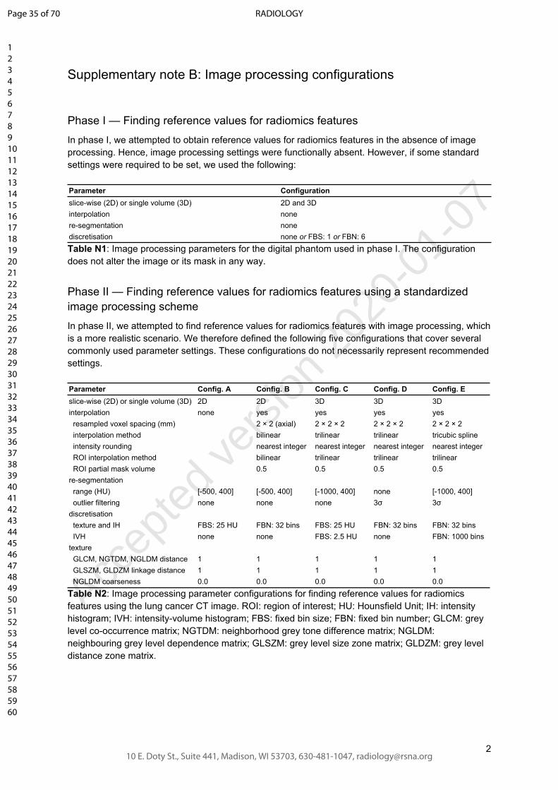
Supplementary note B: Image processing configurations

Phase I — Finding reference values for radiomics features

In phase I, we attempted to obtain reference values for radiomics features in the absence of image processing. Hence, image processing settings were functionally absent. However, if some standard settings were required to be set, we used the following:

Parameter Configurationslice-wise (2D) or single volume (3D) 2D and 3Dinterpolation nonere-segmentation nonediscretisation none or FBS: 1 or FBN: 6

Table N1: Image processing parameters for the digital phantom used in phase I. The configuration does not alter the image or its mask in any way.

Phase II — Finding reference values for radiomics features using a standardized image processing scheme

In phase II, we attempted to find reference values for radiomics features with image processing, which is a more realistic scenario. We therefore defined the following five configurations that cover several commonly used parameter settings. These configurations do not necessarily represent recommended settings.

Parameter Config. A Config. B Config. C Config. D Config. Eslice-wise (2D) or single volume (3D) 2D 2D 3D 3D 3Dinterpolation none yes yes yes yes resampled voxel spacing (mm) 2 × 2 (axial) 2 × 2 × 2 2 × 2 × 2 2 × 2 × 2 interpolation method bilinear trilinear trilinear tricubic spline intensity rounding nearest integer nearest integer nearest integer nearest integer ROI interpolation method bilinear trilinear trilinear trilinear ROI partial mask volume 0.5 0.5 0.5 0.5re-segmentation range (HU) [-500, 400] [-500, 400] [-1000, 400] none [-1000, 400] outlier filtering none none none 3σ 3σdiscretisation texture and IH FBS: 25 HU FBN: 32 bins FBS: 25 HU FBN: 32 bins FBN: 32 bins IVH none none FBS: 2.5 HU none FBN: 1000 binstexture GLCM, NGTDM, NGLDM distance 1 1 1 1 1 GLSZM, GLDZM linkage distance 1 1 1 1 1 NGLDM coarseness 0.0 0.0 0.0 0.0 0.0

Table N2: Image processing parameter configurations for finding reference values for radiomics features using the lung cancer CT image. ROI: region of interest; HU: Hounsfield Unit; IH: intensity histogram; IVH: intensity-volume histogram; FBS: fixed bin size; FBN: fixed bin number; GLCM: grey level co-occurrence matrix; NGTDM: neighborhood grey tone difference matrix; NGLDM: neighbouring grey level dependence matrix; GLSZM: grey level size zone matrix; GLDZM: grey level distance zone matrix.

Page 35 of 70


RADIOLOGY

123456789101112131415161718192021222324252627282930313233343536373839404142434445464748495051525354555657585960

Accep

ted ve

rsion

2020

-01-07

3

Phase III — Validation

In phase III, the research teams validated the software implementation of standardized features by assessing reproducibility of standardized radiomics features against a new dataset consisting of CT, 18F-FDG-PET and T1-weighted MR imaging, with a predefined image processing configuration. This dataset was preprocessed to ensure that image processing steps that were not investigated during phase II could not affect reproducibility.

Therefore, prior to validation, PET imaging was converted to body-weight corrected SUV, cropped 50 mm around the GTV ROI and exported to DICOM and NIfTI formats.

T1-weighted MR images were bias-field corrected using the N4 algorithm (1) implemented in ITK 5.0.1, using 3 fitting levels, a maximum of 100 iterations at each level and a convergence threshold of 0.001. Subsequently, the images were normalized on subcutaneous fat intensity to increase comparability between the different MR images, as follows. The 95th percentile of the intensities within the patient mask (i.e. tissue voxels) were used to indicate subcutaneous fat. This was verified for all patients. Afterwards, the image intensities were normalized through linear mapping so that 1000 corresponds to the subcutaneous fat intensity in the original image, and 0 corresponds to 0 in the original image. Next, the images were cropped 50 mm around the GTV ROI. The values in the normalized image were then converted to integers prior to export as DICOM and NIfTI formats.

CT images did not undergo any pre-processing and were exported directly to DICOM and NIfTI formats after cropping to 50 mm around the GTV ROI.

The exported datasets were then shared with the research teams, who extracted feature values according to a modality-specific configuration. These configurations are shown below. Note that these configurations are not necessarily recommended, but are well-adjusted to the available imaging data.

Page 36 of 70


RADIOLOGY

123456789101112131415161718192021222324252627282930313233343536373839404142434445464748495051525354555657585960

Accep

ted ve

rsion

2020

-01-07

4

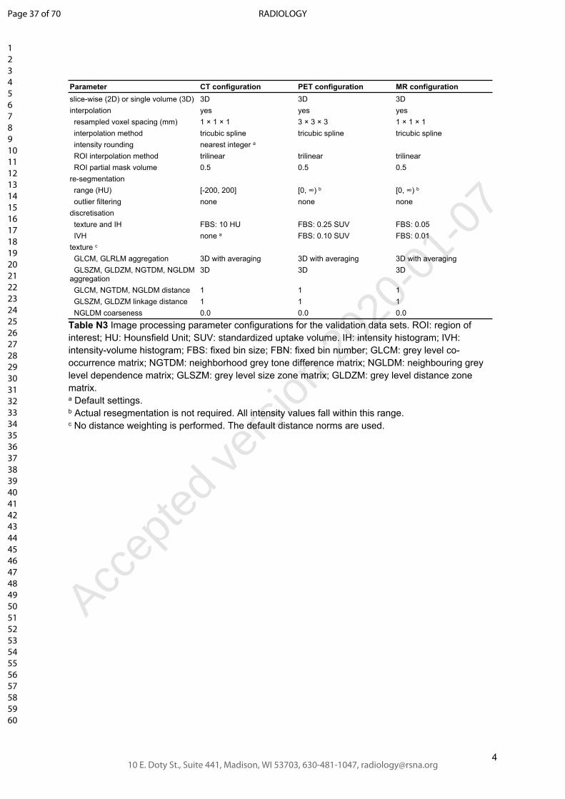
Parameter CT configuration PET configuration MR configurationslice-wise (2D) or single volume (3D) 3D 3D 3Dinterpolation yes yes yes resampled voxel spacing (mm) 1 × 1 × 1 3 × 3 × 3 1 × 1 × 1 interpolation method tricubic spline tricubic spline tricubic spline intensity rounding nearest integer a

ROI interpolation method trilinear trilinear trilinear ROI partial mask volume 0.5 0.5 0.5re-segmentation range (HU) [-200, 200] [0, ∞) b [0, ∞) b

outlier filtering none none nonediscretisation texture and IH FBS: 10 HU FBS: 0.25 SUV FBS: 0.05 IVH none a FBS: 0.10 SUV FBS: 0.01texture c

GLCM, GLRLM aggregation 3D with averaging 3D with averaging 3D with averaging GLSZM, GLDZM, NGTDM, NGLDM aggregation

3D 3D 3D

GLCM, NGTDM, NGLDM distance 1 1 1 GLSZM, GLDZM linkage distance 1 1 1 NGLDM coarseness 0.0 0.0 0.0

Table N3 Image processing parameter configurations for the validation data sets. ROI: region of interest; HU: Hounsfield Unit; SUV: standardized uptake volume. IH: intensity histogram; IVH: intensity-volume histogram; FBS: fixed bin size; FBN: fixed bin number; GLCM: grey level co-occurrence matrix; NGTDM: neighborhood grey tone difference matrix; NGLDM: neighbouring grey level dependence matrix; GLSZM: grey level size zone matrix; GLDZM: grey level distance zone matrix.a Default settings.b Actual resegmentation is not required. All intensity values fall within this range.c No distance weighting is performed. The default distance norms are used.

Page 37 of 70


RADIOLOGY

123456789101112131415161718192021222324252627282930313233343536373839404142434445464748495051525354555657585960

Accep

ted ve

rsion

2020

-01-07

5

Supplementary note C: Tolerance margins

Different algorithm choices, rounding errors and other issues may lead to minor deviations from the reference value of radiomics features. These do not constitute errors or lack of compliance, but should be accounted for regardless. Different features display varying sensitivity to minor perturbations. Some, such as the mean intensity are relatively stable, but others may vary to a greater extent.

Tolerance was determined for the morphological features in phase I and for all features in phase II. In phase I, tolerance was required since different volume meshing algorithms were found to produce slightly different meshes. Differences in meshes lead to deviations in volume and surface area which are propagated into other morphological features. A narrow tolerance of 0.5% of the reference value was used. For other features no tolerance margin was allowed, as these followed mathematically exact definitions.

In phase II, image processing may lead to minor deviations in feature values. As the response of radiomics features to such perturbations varies and cannot be easily translated into a relative tolerance, we perturbed the image and region of interest mask prior to the interpolation step by rotation and translation in the xy-plane with growth and shrinkage of the region of interest (2):

● Rotation: from -15° to 15° in 5° steps.● Translation: permutations of 0.0, 0.25, 0.50 and 0.75 times the voxel spacing in the xy-plane.● Growth and shrinkage: 2 mm growth, original size and 2 mm shrinkage.

Thus 336 values were produced for each feature using the MIRP software (3). The tolerance margin is then set to 5% of the interquartile range.

A separate spreadsheet is appended to the main manuscript. This file contains the reference values and the tolerance margins of all radiomics features obtained from the digital phantom and those obtained from the lung cancer CT image under five image processing configurations.

Page 38 of 70


RADIOLOGY

123456789101112131415161718192021222324252627282930313233343536373839404142434445464748495051525354555657585960

Accep

ted ve

rsion

2020

-01-07

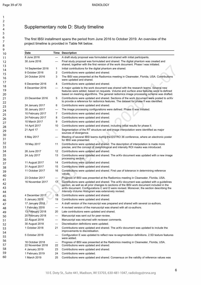
6

Supplementary note D: Study timeline

The first IBSI installment spans the period from June 2016 to October 2019. An overview of the project timeline is provided in Table N4 below.

Date Time Description8 June 2016 — A draft study proposal was formulated and shared with initial participants.30 June 2016 — Final study proposal was formulated and shared. The digital phantom was created and

shared, together with the first version of the work document. Phase I was initiated.14 September 2016 1 Initial contributions for the digital phantom are shared.9 October 2016 2 Contributions were updated and shared.24 October 2016 3 The IBSI was presented at the Radiomics meeting in Clearwater, Florida, USA. Contributions

were updated and shared.6 December 2016 4 Contributions were updated and shared.8 December 2016 — A major update to the work document was shared with the research teams. Several new

features were added, based on requests. Volume and surface area features were re-defined based on meshing algorithms. The general radiomics image processing scheme was drafted.

23 December 2016 5 Contributions were updated and shared. Sections of the work document were posted to arXiv to provide a reference for radiomics features. The dataset for phase II was identified.

24 January 2017 6 Contributions were updated and shared.30 January 2017 — The image processing configurations were defined. Phase II was initiated.10 February 2017 7 Contributions were updated and shared.24 February 2017 8 Contributions were updated and shared.10 March 2017 9 Contributions were updated and shared.14 April 2017 10 Contributions were updated and shared, including initial results for phase II.21 April 17 — Segmentation of the RT structure set and image interpolation were identified as major

sources of divergence.6 May 2017 — Meeting of several IBSI teams during the ESTRO 36 conference, where an electronic poster

for IBSI was presented.19 May 2017 11 Contributions were updated and shared. The description of interpolation is made more

precise, and the concept of morphological and intensity ROI masks was introduced.26 June 2017 12 Contributions were updated and shared.24 July 2017 13 Contributions were updated and shared. The arXiv document was updated with a new image

processing section.11 August 2017 14 Contributions were updated and shared.31 August 2017 15 Contributions were updated and shared.11 October 2017 16 Contributions were updated and shared. First use of tolerance in determining reference

values.23 October 2017 — Progress of IBSI was presented at the Radiomics meeting in Clearwater, Florida, USA.16 November 2017 17 Contributions were updated and shared. The arXiv document was updated with a guidelines

section, as well as all prior changes to sections of the IBSI work document included in the arXiv document. Configurations C and D were revised. Moreover, the section describing the Intensity-Volume Histogram was extensively revised.

4 December 2017 18 Contributions were updated and shared.5 January 2018 19 Contributions were updated and shared.17 January 2018 — A draft version of the manuscript was prepared and shared with several co-authors.1 February 2018 — A revised version of the manuscript was shared with all co-authors.13 February 2018 20 Late contributions were updated and shared.20 February 2018 — Manuscript was sent out for peer-review.22 August 2018 — Manuscript was returned with reviewer comments.30 August 2018 — Discretisation definitions were updated.1 October 2018 21 Contributions were updated and shared. The arXiv document was updated to include the

improvements to discretisation.5 October 2018 — Configuration E was updated to reflect new re-segmentation definitions. 2.5D texture features

were added.16 October 201822 November 2018

—22

Progress of IBSI was presented at the Radiomics meeting in Clearwater, Florida, USA.Contributions were updated and shared.

4 January 2019 23 Contributions were updated and shared.1 February 2019 24 Contributions were updated.1 March 2019 25 Contributions were updated and shared. Consensus on the validity of reference values was

Page 39 of 70


RADIOLOGY

123456789101112131415161718192021222324252627282930313233343536373839404142434445464748495051525354555657585960

Accep

ted ve

rsion

2020

-01-07

7

found to be sufficient to halt the iterative standardization process.4 April 2019 — A completely revised version of the manuscript was shared with all co-authors.16 May 2019 — The arXiv document was updated to include tables of reference values.23 May 2019 — Manuscript was sent out for peer-review.6 August 2019 — Review comments were received.4 September 2019 — The validation phase (III) was started using new datasets deriving from CT, PET and MR

imaging.14 October 2019 — All validation results were collected and parsed.22 October 2019 — The revised manuscript was submitted for peer-review.9 December 2019 — A second revision was submitted.

Table N1: Overview of the project timeline with main events. The time points may be found in figures and tables in this study.

Page 40 of 70


RADIOLOGY

123456789101112131415161718192021222324252627282930313233343536373839404142434445464748495051525354555657585960

Accep

ted ve

rsion

2020

-01-07

8

Supplementary note E: Research team information

In total, 25 research teams voluntarily participated in the IBSI. Details are found in Table N5 below. Participation criteria were as follows:

● A team developed their own software for image processing and feature computation.● A team would participate in at least one phase of the study.

The initial set of teams was invited directly as they were either present at the ESTRO radiomics workshop in 2016, were known to be interested, or had done some early work in the direction of standardization. Teams then also referred to other potentially interested teams of researchers, who then joined as well. Beyond the initial set, most teams joined after learning of the IBSI at conferences or workshops, through colleagues, or after encountering the arXiv preprint. Several open-source developers were directly invited (e.g. LifeX). Recruitment was open at any point during the study.

Figure N1: Details concerning the teams and their software implementations. (A) Graph showing the number of teams involved in each phase. One team retired because they switched to software developed by another team. (B) Source code and software availability, and (C) the main programming languages of the research teams..

As shown in Figure N1, eleven of the twenty-five teams developed publicly available software implementations: McGill (4–6), MITK (7), Pyradiomics (8), CERR (9), QuantImage (10), QIFE (11), RaCaT (12), CaPTk (13,14), LIFEx (15), SERA (16) and MIRP (3). The remainder used in-house software.

Team Institution Main developer First entry Language Availability

Brest (BCOM) INSERM Brest Taman Upadhaya 1 C++ in-house

Brest (MaCha) INSERM Brest Marie-CharlotteDesseroit, Baptiste Laurent

1 C++ in-house

Gemelli Fondazione Policlinico Universitario Agostino Gemelli

Jacopo Lenkowicz 1 R in-house

LUMC Leiden University Medical Center (LUMC), VU University Medical Center

Floris H.P. van Velden, Ronald Boellaard

1 IDL in-house

McGill McGill University Martin Vallières 1 MATLAB open source1

MITK German Cancer Research Center (DKFZ)

Michael Götz, FabianIsensee, Jonas Scherer

1 C++ open source2

Moffitt Moffitt Cancer Center Mahmoud A. Abdalah 1 C++ in-house

NKIa the Netherlands Cancer Institute (NKI) Cuong Viet Dinh 1 C++ in-house

MIRP OncoRay – National Center for Radiation Research in Oncology

Alex Zwanenburg, Stefan Leger

1 Python open source3

Tuebingen University of Tübingen 1 Python in-house

1 https://github.com/mvallieres/radiomics-develop2 http://mitk.org3 https://github.com/oncoray/mirp

Page 41 of 70


RADIOLOGY

123456789101112131415161718192021222324252627282930313233343536373839404142434445464748495051525354555657585960

Accep

ted ve

rsion

2020

-01-07

buvat

Barrer

buvat

Note

LIFEx

9

UMCG (van Dijk) University Medical Center Groningen (UMCG)

Lisanne V. van Dijk 1 MATLAB in-house

USZ University of Zurich Marta Bogowicz 1 Python in-house

MAASTRO Maastricht University Medical Centre+ Ralph T.H. Leijenaar 2 MATLAB in-house

Cardiff Cardiff University Philip Whybra 4 MATLAB in-house

UMCG (Beukinga) University Medical Center Groningen (UMCG)

Roelof J. Beukinga 8 MATLAB in-house

Pyradiomics the Netherlands Cancer Institute (NKI), Maastricht University, Dana-Farber Cancer Institute

Joost van Griethuysen, Andriy Fedorov

9 Python open source4

UCSF University of California, San Francisco (UCSF)

Olivier Morin 10 Python in-house

CERR Memorial Sloan Kettering Cancer Center

Aditya Apte 11 MATLAB open source5

SERA Johns Hopkins University Saeed Ashrafinia 12 MATLAB open source6

QuantImage University of Applied Sciences Western Switzerland (HES-SO)

Adrien Depeursinge, Vincent Andrearczyk

18 MATLAB web-based7

QIFE Stanford University Sebastian Echegaray, Sarah Mattonen

20 MATLAB open source8

RaCaT University Medical Center Groningen (UMCG)

Elisabeth Pfaehler 21 C++ open source9

CaPTk University of Pennsylvania Sarthak Pati, Sung Min Ha

21 C++ open source10

LIFEx Université Paris Saclay Christophe Nioche 21 Java freeware11

KCL King’s College London Muhammad Siddique 22 MATLAB in-house

Table N5: Details regarding the participating research teams. The institution is the main institution at which the developers worked, which were either universities, university medical centers or research institutions. The main developers were primarily responsible for developing, testing and adapting source code during the course of the project. The first entry is the time point at which the team’s contribution was first incorporated.a This research team retired after stopping development of their software and switching to the software developed by another participant (pyradiomics).

4 https://github.com/Radiomics/pyradiomics5 https://github.com/cerr/CERR6 https://github.com/ashrafinia/SERA7 https://radiomics.hevs.ch/8 https://github.com/riipl/3d_qifp9 https://github.com/ellipfaehlerUMCG/RaCat10 https://github.com/CBICA/CaPTk11 https://www.lifexsoft.org/

Page 42 of 70


RADIOLOGY

123456789101112131415161718192021222324252627282930313233343536373839404142434445464748495051525354555657585960

Accep

ted ve

rsion

2020

-01-07

10

Supplementary note F: Coverage of features per research team

Research teams were not required to implement every feature and support all image processing options. This led to a feature coverage that varied between teams, which is shown in Figure N2 below. Nine teams implemented >50% of the features, and five teams implemented > 95% of the features.

Figure N2: Feature coverage of each research team at the final analysis time point for phases I and II. Features were extracted from the digital phantom (phase I) and from a CT lung cancer image using image processing configurations A-E (phase II). “no ref. value” indicates that there was no consensus on a reference value of a feature, i.e. the number of matching values produced by the teams was < 3, or matching values were produced by ≤50% of contributing teams. “Deviating” indicates that a feature was implemented, but deviated from the reference value. “Matching” indicates that a feature was implemented and the reference value could be reproduced by the team. The number of features is different for each dataset due to different availability of texture matrix aggregation methods: 487 (digital phantom), 351 (configurations A, B), and 215 (configurations C-E).

Page 43 of 70


RADIOLOGY

123456789101112131415161718192021222324252627282930313233343536373839404142434445464748495051525354555657585960

Accep

ted ve

rsion

2020

-01-07

11

Supplementary note G: Number of unique institutions and consensus

Research teams that are part of the same institution may potentially share the same code. We did not find any evidence to support this. Four teams shared an institution and developed their software using the same language. Concurrent submissions from these teams showed differences in feature values, which is evidence against using the same code. However, even if the same code was being used by multiple teams within an institution, the effect on consensus is weak, as shown below.

As shown in Table N6 below, the minimum number of unique top-level institutions with matching values was:

● 3 for features with moderate consensus.● 5 for features with strong consensus.● 8 for features with very strong consensus.

Note that consensus on the validity of reference values is based on the number of research teams that reproduced the reference value: 3: weak; 3-5: moderate; 6-9: strong; ≥ 10 very strong. Hence the same number of unique top-level institutions may appear for multiple consensus levels.

Consensus level Unique top-level institutions Number of features

weak 1 16

weak 2 5

moderate 3 20

moderate 4 56

moderate 5 54

strong 5 224

strong 6 559

strong 7 390

strong 8 199

strong 9 14

very strong 8 2

very strong 9 126

very strong 10 19

very strong 11 27

very strong 12 30

very strong 13 27

very strong 14 30

very strong 15 10

very strong 16 16

very strong 17 2

very strong 18 4

very strong 19 2

very strong 20 2

Table N6: The number of unique top-level institutions for features grouped by the level of consensus on the validity of their reference values.

Page 44 of 70


RADIOLOGY

123456789101112131415161718192021222324252627282930313233343536373839404142434445464748495051525354555657585960

Accep

ted ve

rsion

2020

-01-07

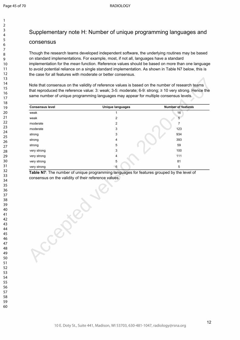
12

Supplementary note H: Number of unique programming languages and

consensus

Though the research teams developed independent software, the underlying routines may be based on standard implementations. For example, most, if not all, languages have a standard implementation for the mean function. Reference values should be based on more than one language to avoid potential reliance on a single standard implementation. As shown in Table N7 below, this is the case for all features with moderate or better consensus.

Note that consensus on the validity of reference values is based on the number of research teams that reproduced the reference value: 3: weak; 3-5: moderate; 6-9: strong; ≥ 10 very strong. Hence the same number of unique programming languages may appear for multiple consensus levels.

Consensus level Unique languages Number of features

weak 1 16

weak 2 5

moderate 2 7

moderate 3 123

strong 3 934

strong 4 393

strong 5 59

very strong 3 100

very strong 4 111

very strong 5 81

very strong 6 5

Table N7: The number of unique programming languages for features grouped by the level of consensus on the validity of their reference values.

Page 45 of 70


RADIOLOGY

123456789101112131415161718192021222324252627282930313233343536373839404142434445464748495051525354555657585960

Accep

ted ve

rsion

2020

-01-07

13

Supplementary note I: Features with a weak consensus

Moderate or better consensus could not be established for every feature. These features are the same across the different data sets, namely the area and volume densities derived from the minimum volume enclosing ellipsoid (MVEE) and the oriented minimum bounding box (OMBB). OMBB and MVEE both rely on complex algorithmic optimisers that are not commonly implemented. The OMBB for the digital phantom is easily determined, as it is the same as the axis-aligned bounding box.

Data set Feature Matches Dissent

digital phantom Area density (MVEE) 1 3

digital phantom Volume density (MVEE) 1 3

configuration A Area under the IVH curve 3 3

configuration A Area density (MVEE) 2 1

configuration A Area density (OMBB) 1 3

configuration A Volume density (MVEE) 1 2

configuration A Volume density (OMBB) 1 3

configuration B Area under the IVH curve 3 3

configuration B Area density (MVEE) 1 2

configuration B Area density (OMBB) 1 3

configuration B Volume density (MVEE) 1 3

configuration B Volume density (OMBB) 1 3

configuration C Area density (MVEE) 1 2

configuration C Area density (OMBB) 1 3

configuration C Volume density (MVEE) 1 3

configuration C Volume density (OMBB) 2 2

configuration D Area density (MVEE) 1 2

configuration D Area density (OMBB) 2 2

configuration D Volume density (MVEE) 1 2

configuration D Volume density (OMBB) 2 2

configuration E Volume density (MVEE) 1 3

configuration E Area density (MVEE) 1 4

configuration E Volume density (OMBB) 2 2

Table N8: Features with a weak level of consensus. These are features describing morphological features based on the oriented minimum bounding box (OMBB) and the minimum volume enclosing ellipsoid (MVEE). The number of matches and the number of dissenting research teams is shown.

Page 46 of 70


RADIOLOGY

123456789101112131415161718192021222324252627282930313233343536373839404142434445464748495051525354555657585960

Accep

ted ve

rsion

2020

-01-07

14

Supplementary note J: Detailed information regarding feature

implementations

Table N9 below contains information concerning each feature at its initial introduction and after the final iteration:

● The number of research teams that were able to reproduce the tentative reference value of a feature.

● The number of teams that contributed a value.● The total number of teams.

First entry Final entrymatching implem. total matching implem. total

Morphological features

Volume (mesh) 8 10 12 11 12 24

Volume (voxel counting) 13 13 17 21 21 24

Surface area (mesh) 1 11 12 11 12 24

Surface to volume ratio 1 11 12 10 12 24

Compactness 1 1 11 12 9 11 24

Compactness 2 1 11 12 9 11 24

Spherical disproportion 1 11 12 9 11 24

Sphericity 1 11 12 10 12 24

Asphericity 0 9 12 8 11 24

Centre of mass shift 7 9 12 15 15 24

Maximum 3D diameter 4 9 12 8 12 24

Major axis length 2 10 12 14 17 24

Minor axis length 2 9 12 11 17 24

Least axis length 2 9 12 11 17 24

Elongation 6 9 12 14 19 24

Flatness 6 9 12 13 18 24

Volume density (AABB) 2 3 14 6 8 24

Area density (AABB) 1 3 14 7 8 24

Volume density (OMBB) 2 2 14 3 3 24

Area density (OMBB) 2 2 14 3 3 24

Volume density (AEE) 2 2 14 5 7 24

Area density (AEE) 2 2 14 5 6 24

Volume density (MVEE) 1 2 14 1 4 24

Area density (MVEE) 1 2 14 1 4 24

Volume density (convex hull) 2 2 14 6 7 24

Area density (convex hull) 2 2 14 7 7 24

Integrated intensity 3 3 14 5 8 24

Moran's I index 2 2 14 7 7 24

Geary's C measure 2 2 14 7 7 24

Local intensity features

Local intensity peak 1 2 14 8 8 24

Global intensity peak 1 2 14 6 7 24

Intensity-based statistical features

Page 47 of 70


RADIOLOGY

123456789101112131415161718192021222324252627282930313233343536373839404142434445464748495051525354555657585960

Accep

ted ve

rsion

2020

-01-07

15

Mean 12 12 12 23 23 24

Variance 6 12 12 14 22 24

Skewness 10 12 12 21 23 24

(Excess) kurtosis 6 12 12 20 23 24

Median 9 10 12 20 20 24

Minimum 11 11 12 23 23 24

10th percentile 9 9 12 18 18 24

90th percentile 5 9 12 12 18 24

Maximum 11 11 12 22 22 24

Interquartile range 8 9 12 20 20 24

Range 10 10 12 19 19 24

Mean absolute deviation 9 10 12 19 19 24

Robust mean absolute deviation 7 9 12 17 17 24

Median absolute deviation 2 2 14 12 12 24

Coefficient of variation 1 2 14 12 14 24

Quartile coefficient of dispersion 2 2 14 12 12 24

Energy 10 10 12 17 17 24

Root mean square 9 9 12 17 17 24

Intensity histogram features

Mean 4 4 14 13 13 24

Variance 2 4 14 9 12 24

Skewness 4 4 14 12 13 24

Kurtosis 3 4 14 12 13 24

Median 3 4 14 11 11 24

Minimum 4 4 14 13 13 24

10th percentile 4 4 14 10 10 24

90th percentile 3 4 14 7 10 24

Maximum 4 4 14 12 12 24

Mode 2 2 14 10 10 24

Interquartile range 3 4 14 11 11 24

Range 4 4 14 11 11 24

Mean absolute deviation 3 4 14 11 11 24

Robust mean absolute deviation 4 4 14 10 10 24

Median absolute deviation 2 2 14 10 10 24

Coefficient of variation 1 2 14 10 10 24

Quartile coefficient of dispersion 2 2 14 10 10 24

Entropy 8 11 12 19 19 24

Uniformity 8 10 12 19 19 24

Maximum histogram gradient 2 2 14 10 10 24

Maximum histogram gradient intensity 2 2 14 8 10 24

Minimum histogram gradient 2 2 14 10 10 24

Minimum histogram gradient intensity 2 2 14 9 10 24

Intensity-volume histogram features

Volume fraction at 10% intensity 2 2 14 10 10 24

Volume fraction at 90% intensity 2 2 14 10 10 24

Intensity at 10% volume 1 2 14 10 10 24

Intensity at 90% volume 1 2 14 10 10 24

Volume fraction difference between 10% and 90% intensity

2 2 14 10 10 24

Intensity difference between 10% and 90% volume 2 2 14 10 10 24

Page 48 of 70


RADIOLOGY

123456789101112131415161718192021222324252627282930313233343536373839404142434445464748495051525354555657585960

Accep

ted ve

rsion

2020

-01-07

16

Area under the IVH curve 1 2 14 8 9 24

Co-occurrence matrix (2D, averaged) features

Joint maximum 2 3 12 10 10 24

Joint average 1 3 12 10 10 24

Joint variance 1 3 12 10 10 24

Joint entropy 2 3 12 10 10 24

Difference average 1 3 12 10 10 24

Difference variance 1 3 12 10 10 24

Difference entropy 1 3 12 10 10 24

Sum average 2 3 12 10 10 24

Sum variance 1 3 12 10 10 24

Sum entropy 1 3 12 10 10 24

Angular second moment 2 3 12 10 10 24

Contrast 2 3 12 10 10 24

Dissimilarity 2 3 12 10 10 24

Inverse difference 1 2 12 10 10 24

Normalized inverse difference 1 2 12 10 10 24

Inverse difference moment 1 3 12 10 10 24

Normalized inverse difference moment 2 3 12 10 10 24

Inverse variance 1 2 12 10 10 24

Correlation 1 3 12 10 10 24

Autocorrelation 2 3 12 10 10 24

Cluster tendency 2 3 12 10 10 24

Cluster shade 2 3 12 10 10 24

Cluster prominence 2 3 12 10 10 24

Information correlation 1 1 3 12 10 10 24


Co-occurrence matrix (2D, slice-merged) features








Sum average 1 1 12 9 9 24

Sum variance 1 1 12 9 9 24

Sum entropy 1 1 12 9 9 24


Contrast 1 1 12 9 9 24











Page 49 of 70


RADIOLOGY

123456789101112131415161718192021222324252627282930313233343536373839404142434445464748495051525354555657585960

Accep

ted ve

rsion

2020

-01-07

17




Co-occurrence matrix (2.5D, direction-merged) features












Contrast 4 4 21 8 8 24














Co-occurrence matrix (2.5D, merged) features












Contrast 4 4 21 8 8 24









Page 50 of 70


RADIOLOGY

123456789101112131415161718192021222324252627282930313233343536373839404142434445464748495051525354555657585960

Accep

ted ve

rsion

2020

-01-07

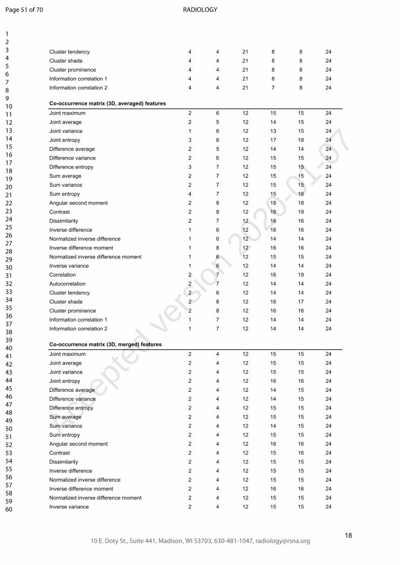
18






Co-occurrence matrix (3D, averaged) features








Sum average 2 7 12 15 15 24

Sum variance 2 7 12 15 15 24

Sum entropy 4 7 12 15 16 24


Contrast 2 8 12 18 19 24














Co-occurrence matrix (3D, merged) features








Sum average 2 4 12 15 15 24

Sum variance 2 4 12 14 15 24

Sum entropy 2 4 12 15 15 24


Contrast 2 4 12 15 16 24







Page 51 of 70


RADIOLOGY

123456789101112131415161718192021222324252627282930313233343536373839404142434445464748495051525354555657585960

Accep

ted ve

rsion

2020

-01-07

19








Run length matrix (2D, averaged) features

Short runs emphasis 1 2 12 10 10 24

Long runs emphasis 1 2 12 10 10 24

Low grey level run emphasis 1 2 12 10 10 24

High grey level run emphasis 1 2 12 10 10 24

Short run low grey level emphasis 1 2 12 10 10 24

Short run high grey level emphasis 1 2 12 10 10 24

Long run low grey level emphasis 1 2 12 10 10 24

Long run high grey level emphasis 1 2 12 10 10 24

Grey level non-uniformity 1 2 12 10 10 24

Normalized grey level non-uniformity 1 1 12 10 10 24

Run length non-uniformity 1 2 12 10 10 24

Normalized run length non-uniformity 1 1 12 10 10 24

Run percentage 1 2 12 10 10 24

Grey level variance 1 2 12 10 10 24

Run length variance 1 2 12 10 10 24

Run entropy 1 2 12 10 10 24

Run length matrix (2D, slice-merged) features
















Run entropy 1 1 12 9 9 24

Run length matrix (2.5D, direction-merged) features








Page 52 of 70


RADIOLOGY

123456789101112131415161718192021222324252627282930313233343536373839404142434445464748495051525354555657585960

Accep

ted ve

rsion

2020

-01-07

20










Run length matrix (2.5D, merged) features

















Run length matrix (3D, averaged) features
















Run entropy 4 5 12 14 14 24

Run length matrix (3D, merged) features






Page 53 of 70


RADIOLOGY

123456789101112131415161718192021222324252627282930313233343536373839404142434445464748495051525354555657585960

Accep

ted ve

rsion

2020

-01-07

21











Run entropy 4 4 12 12 12 24

Size zone matrix (2D) features

Small zone emphasis 1 2 12 9 9 24

Large zone emphasis 1 2 12 9 9 24

Low grey level emphasis 1 2 12 9 9 24

High grey level emphasis 1 2 12 9 9 24

Small zone low grey level emphasis 1 2 12 9 9 24

Small zone high grey level emphasis 1 2 12 9 9 24

Large zone low grey level emphasis 1 2 12 9 9 24

Large zone high grey level emphasis 1 2 12 9 9 24



Zone size non-uniformity 2 2 12 9 9 24

Normalized zone size non-uniformity 1 1 12 9 9 24

Zone percentage 1 2 12 9 9 24


Zone size variance 1 2 12 9 9 24

Zone size entropy 2 2 12 9 9 24

Size zone matrix (2.5D) features

















Size zone matrix (3D) features




Page 54 of 70


RADIOLOGY

123456789101112131415161718192021222324252627282930313233343536373839404142434445464748495051525354555657585960

Accep

ted ve

rsion

2020

-01-07

22














Distance zone matrix (2D) features

Small distance emphasis 1 1 12 7 7 24

Large distance emphasis 1 1 12 7 7 24



Small distance low grey level emphasis 1 1 12 7 7 24

Small distance high grey level emphasis 1 1 12 7 7 24

Large distance low grey level emphasis 1 1 12 7 7 24

Large distance high grey level emphasis 1 1 12 7 7 24



Zone distance non-uniformity 1 1 12 7 7 24

Normalized zone distance non-uniformity 1 1 12 7 7 24



Zone distance variance 1 1 12 7 7 24

Zone distance entropy 1 1 12 7 7 24

Distance zone matrix (2.5D) features

















Distance zone matrix (3D) features


Page 55 of 70


RADIOLOGY

123456789101112131415161718192021222324252627282930313233343536373839404142434445464748495051525354555657585960

Accep

ted ve

rsion

2020

-01-07

23
















Neighborhood grey tone difference matrix (2D) features

Coarseness 1 2 12 8 8 24

Contrast 1 2 12 8 8 24

Busyness 1 2 12 8 8 24

Complexity 1 2 12 8 8 24

Strength 1 2 12 8 8 24

Neighborhood grey tone difference matrix (2.5D) features

Coarseness 3 4 21 7 7 24

Contrast 3 4 21 7 7 24

Busyness 3 4 21 6 7 24

Complexity 4 4 21 6 7 24

Strength 3 4 21 6 7 24

Neighborhood grey tone difference matrix (3D) features

Coarseness 2 7 12 18 18 24

Contrast 2 7 12 17 18 24

Busyness 2 7 12 16 18 24

Complexity 2 7 12 14 17 24

Strength 2 7 12 14 17 24

Neighboring grey level dependence matrix (2D) features

Low dependence emphasis 1 1 12 7 7 24

High dependence emphasis 1 1 12 7 7 24

Low grey level count emphasis 1 1 12 7 7 24

High grey level count emphasis 1 1 12 7 7 24

Low dependence low grey level emphasis 1 1 12 7 7 24

Low dependence high grey level emphasis 1 1 12 7 7 24

High dependence low grey level emphasis 1 1 12 7 7 24

High dependence high grey level emphasis 1 1 12 7 7 24



Dependence count non-uniformity 1 1 12 7 7 24

Normalized dependence count non-uniformity 1 1 12 7 7 24

Dependence count percentage 1 1 12 6 6 24


Page 56 of 70


RADIOLOGY

123456789101112131415161718192021222324252627282930313233343536373839404142434445464748495051525354555657585960

Accep

ted ve

rsion

2020

-01-07

24

Dependence count variance 1 1 12 7 7 24

Dependence count entropy 1 1 12 7 7 24

Dependence count energy 1 1 14 7 7 24

Neighboring grey level dependence matrix (2.5D) features


















Neighboring grey level dependence matrix (3D) features


















Table N9: Details regarding the number of radiomic feature implementations and consensus on the validity of tentative reference values at the initial and final time points for the digital phantom in phase I. Note that while at the final time point the number of research teams is the same for every feature, this is not the case at the initial time point as some radiomics features were introduced later during the iterative process.

Page 57 of 70


RADIOLOGY

123456789101112131415161718192021222324252627282930313233343536373839404142434445464748495051525354555657585960

Accep

ted ve

rsion

2020

-01-07

25

Supplementary note K: Feature reproducibility in the validation cohort

For validation, research teams extracted features from CT, 18F-FDG-PET and T1-weighted MR images of 51 patients according to the configurations in supplementary note B. Standardization of each feature by a team was first assessed by determining whether the team could demonstrate that they were able to reproduce the respective reference values under configurations C, D and E (established in phase II). If this was the case, the standardized feature was then used to compute a two-way random effects, single rater, absolute agreement intraclass correlation coefficient (ICC). These ICC values and their 95% confidence intervals are shown in Table N10 below.

CT PET MRI

Morphological features

Volume (mesh) 0.976 [0.964, 0.985] 0.976 [0.964, 0.985] 0.968 [0.952, 0.980]

Volume (voxel counting) 1.000 [1.000, 1.000] 1.000 [1.000, 1.000] 0.999 [0.999, 1.000]

Surface area (mesh) 1.000 [1.000, 1.000] 1.000 [1.000, 1.000] 0.999 [0.999, 0.999]

Surface to volume ratio 1.000 [1.000, 1.000] 1.000 [1.000, 1.000] 0.999 [0.999, 1.000]

Compactness 1 1.000 [1.000, 1.000] 1.000 [0.999, 1.000] 0.995 [0.993, 0.997]

Compactness 2 1.000 [0.999, 1.000] 0.999 [0.999, 1.000] 0.994 [0.990, 0.996]

Spherical disproportion 1.000 [1.000, 1.000] 1.000 [0.999, 1.000] 0.995 [0.993, 0.997]

Sphericity 1.000 [1.000, 1.000] 1.000 [0.999, 1.000] 0.995 [0.992, 0.997]

Asphericity 1.000 [1.000, 1.000] 0.999 [0.999, 1.000] 0.995 [0.992, 0.997]

Centre of mass shift 1.000 [1.000, 1.000] 0.999 [0.998, 0.999] 0.989 [0.984, 0.993]

Maximum 3D diameter 0.997 [0.996, 0.998] 0.997 [0.995, 0.998] 0.990 [0.984, 0.994]

Major axis length 1.000 [1.000, 1.000] 0.999 [0.999, 1.000] 0.993 [0.990, 0.996]

Minor axis length 1.000 [0.999, 1.000] 0.999 [0.999, 1.000] 0.997 [0.996, 0.998]

Least axis length 1.000 [1.000, 1.000] 1.000 [1.000, 1.000] 1.000 [1.000, 1.000]

Elongation 0.999 [0.999, 1.000] 0.999 [0.998, 0.999] 0.995 [0.993, 0.997]

Flatness 1.000 [0.999, 1.000] 0.999 [0.999, 1.000] 0.992 [0.988, 0.995]

Volume density (AABB) 0.999 [0.998, 0.999] 0.989 [0.984, 0.993] 0.973 [0.959, 0.983]

Area density (AABB) 0.998 [0.997, 0.999] 0.989 [0.983, 0.993] 0.974 [0.961, 0.984]

Volume density (OMBB) NS NS NS

Area density (OMBB) NS NS NS

Volume density (AEE) 1.000 [1.000, 1.000] 1.000 [0.999, 1.000] 1.000 [1.000, 1.000]

Area density (AEE) 1.000 [1.000, 1.000] 0.999 [0.999, 0.999] 1.000 [1.000, 1.000]

Volume density (MVEE) NS NS NS

Area density (MVEE) NS NS NS

Volume density (convex hull) 1.000 [1.000, 1.000] 1.000 [1.000, 1.000] 1.000 [1.000, 1.000]

Area density (convex hull) 1.000 [1.000, 1.000] 1.000 [0.999, 1.000] 1.000 [1.000, 1.000]

Integrated intensity 0.942 [0.915, 0.963] 0.987 [0.980, 0.992] 0.981 [0.971, 0.988]

Moran's I index NA NA NA

Geary's C measure NA NA NA

Local intensity features

Local intensity peak 1.000 [1.000, 1.000] 0.967 [0.949, 0.980] 0.971 [0.955, 0.982]

Global intensity peak 1.000 [1.000, 1.000] 0.999 [0.999, 1.000] 1.000 [1.000, 1.000]

Intensity-based statistics featuresMean 0.999 [0.999, 1.000] 0.999 [0.999, 1.000] 0.997 [0.995, 0.998]

Variance 1.000 [1.000, 1.000] 0.999 [0.999, 1.000] 0.997 [0.995, 0.998]

Skewness 1.000 [1.000, 1.000] 0.997 [0.996, 0.998] 0.992 [0.988, 0.995]

(Excess) kurtosis 0.994 [0.992, 0.996] 0.997 [0.996, 0.998] 0.990 [0.986, 0.994]

Page 58 of 70


RADIOLOGY

123456789101112131415161718192021222324252627282930313233343536373839404142434445464748495051525354555657585960

Accep

ted ve

rsion

2020

-01-07

26

Median 0.998 [0.998, 0.999] 0.999 [0.999, 1.000] 0.997 [0.995, 0.998]

Minimum 0.990 [0.985, 0.994] 0.972 [0.958, 0.982] 0.983 [0.975, 0.989]

10th percentile 1.000 [1.000, 1.000] 0.999 [0.998, 0.999] 0.997 [0.996, 0.998]

90th percentile 0.999 [0.999, 1.000] 0.999 [0.999, 1.000] 0.998 [0.997, 0.999]

Maximum 0.998 [0.997, 0.999] 0.991 [0.986, 0.994] 0.993 [0.990, 0.996]

Interquartile range 0.999 [0.999, 0.999] 0.999 [0.999, 0.999] 0.996 [0.994, 0.997]

Range 0.994 [0.990, 0.996] 0.990 [0.986, 0.994] 0.990 [0.985, 0.994]

Mean absolute deviation 1.000 [1.000, 1.000] 0.999 [0.999, 1.000] 0.996 [0.994, 0.998]

Robust mean absolute deviation 1.000 [0.999, 1.000] 0.928 [0.895, 0.954] 0.995 [0.993, 0.997]

Median absolute deviation 1.000 [1.000, 1.000] 0.999 [0.999, 1.000] 0.996 [0.994, 0.998]

Coefficient of variation 1.000 [1.000, 1.000] 1.000 [0.999, 1.000] 0.997 [0.995, 0.998]

Quartile coefficient of dispersion 1.000 [1.000, 1.000] 0.998 [0.997, 0.999] 0.998 [0.997, 0.999]

Energy 1.000 [1.000, 1.000] 1.000 [1.000, 1.000] 1.000 [1.000, 1.000]

Root mean square 0.999 [0.998, 0.999] 0.999 [0.999, 0.999] 0.997 [0.995, 0.998]

Intensity histogram featuresMean 1.000 [0.999, 1.000] 0.999 [0.999, 1.000] 0.997 [0.995, 0.998]

Variance 1.000 [1.000, 1.000] 0.999 [0.999, 1.000] 0.997 [0.995, 0.998]

Skewness 1.000 [1.000, 1.000] 0.999 [0.999, 0.999] 0.998 [0.997, 0.999]

(Excess) kurtosis 1.000 [1.000, 1.000] 0.998 [0.997, 0.999] 0.998 [0.997, 0.999]

Median 1.000 [0.999, 1.000] 0.999 [0.999, 0.999] 0.997 [0.996, 0.998]

Minimum 0.992 [0.989, 0.995] 0.940 [0.912, 0.962] 0.984 [0.977, 0.990]

10th percentile 1.000 [1.000, 1.000] 0.996 [0.993, 0.997] 0.997 [0.995, 0.998]

90th percentile 0.977 [0.965, 0.985] 0.998 [0.996, 0.998] 0.993 [0.990, 0.996]

Maximum 0.996 [0.995, 0.998] 0.989 [0.984, 0.993] 0.993 [0.990, 0.996]

Mode 1.000 [1.000, 1.000] 1.000 [0.999, 1.000] 1.000 [0.999, 1.000]

Interquartile range 1.000 [1.000, 1.000] 0.997 [0.996, 0.998] 0.982 [0.973, 0.989]

Range 0.994 [0.991, 0.996] 0.990 [0.984, 0.993] 0.990 [0.985, 0.994]

Mean absolute deviation 1.000 [1.000, 1.000] 0.999 [0.999, 1.000] 0.996 [0.994, 0.998]

Robust mean absolute deviation 1.000 [1.000, 1.000] 1.000 [0.999, 1.000] 0.996 [0.993, 0.997]

Median absolute deviation 1.000 [1.000, 1.000] 0.999 [0.999, 1.000] 0.996 [0.995, 0.998]

Coefficient of variation 1.000 [1.000, 1.000] 1.000 [0.999, 1.000] 0.997 [0.995, 0.998]

Quartile coefficient of dispersion 1.000 [1.000, 1.000] 0.981 [0.971, 0.988] 0.993 [0.990, 0.996]

Entropy 1.000 [1.000, 1.000] 0.999 [0.999, 1.000] 0.995 [0.993, 0.997]

Uniformity 1.000 [1.000, 1.000] 1.000 [0.999, 1.000] 0.996 [0.994, 0.997]

Maximum histogram gradient 1.000 [1.000, 1.000] 0.987 [0.981, 0.992] 0.999 [0.998, 0.999]

Maximum histogram gradient intensity 0.999 [0.999, 1.000] 0.897 [0.847, 0.934] 0.999 [0.999, 1.000]

Minimum histogram gradient 1.000 [1.000, 1.000] 0.992 [0.987, 0.995] 0.999 [0.999, 0.999]

Minimum histogram gradient intensity 0.999 [0.999, 0.999] 1.000 [1.000, 1.000] 0.999 [0.998, 0.999]

Intensity-volume histogram featuresVolume fraction at 10% intensity 1.000 [1.000, 1.000] 0.989 [0.983, 0.994] 1.000 [1.000, 1.000]

Volume fraction at 90% intensity 0.882 [0.829, 0.923] 0.830 [0.760, 0.889] 0.872 [0.816, 0.917]

Intensity at 10% volume 0.999 [0.999, 1.000] 0.999 [0.999, 0.999] 0.998 [0.997, 0.999]

Intensity at 90% volume 1.000 [1.000, 1.000] 0.995 [0.992, 0.997] 1.000 [1.000, 1.000]

Volume fraction difference between 10% and 90% intensity

1.000 [1.000, 1.000] 0.985 [0.978, 0.991] 1.000 [1.000, 1.000]

Intensity difference between 10% and 90% volume 1.000 [1.000, 1.000] 0.998 [0.997, 0.999] 0.997 [0.996, 0.998]

Area under the IVH curve NS NS NS

Co-occurrence matrix featuresJoint maximum 1.000 [1.000, 1.000] 0.999 [0.999, 1.000] 0.997 [0.996, 0.998]

Joint average 0.999 [0.999, 1.000] 0.999 [0.999, 1.000] 0.997 [0.995, 0.998]

Page 59 of 70


RADIOLOGY

123456789101112131415161718192021222324252627282930313233343536373839404142434445464748495051525354555657585960

Accep

ted ve

rsion

2020

-01-07

27

Joint variance 1.000 [1.000, 1.000] 0.999 [0.999, 1.000] 0.996 [0.995, 0.998]

Joint entropy 1.000 [1.000, 1.000] 0.999 [0.999, 1.000] 0.996 [0.994, 0.997]

Difference average 1.000 [1.000, 1.000] 0.999 [0.999, 0.999] 0.996 [0.995, 0.998]

Difference variance 1.000 [1.000, 1.000] 0.999 [0.998, 0.999] 0.998 [0.996, 0.998]

Difference entropy 1.000 [1.000, 1.000] 0.999 [0.999, 0.999] 0.997 [0.995, 0.998]

Sum average 0.999 [0.999, 1.000] 0.999 [0.999, 0.999] 0.997 [0.995, 0.998]

Sum variance 1.000 [1.000, 1.000] 0.999 [0.999, 1.000] 0.996 [0.994, 0.998]

Sum entropy 1.000 [1.000, 1.000] 0.999 [0.999, 1.000] 0.996 [0.993, 0.997]

Angular second moment 1.000 [1.000, 1.000] 1.000 [1.000, 1.000] 0.995 [0.992, 0.997]

Contrast 1.000 [1.000, 1.000] 0.999 [0.999, 1.000] 0.997 [0.996, 0.998]

Dissimilarity 1.000 [1.000, 1.000] 0.999 [0.999, 0.999] 0.996 [0.995, 0.998]

Inverse difference 1.000 [1.000, 1.000] 0.999 [0.999, 1.000] 0.998 [0.996, 0.998]

Normalized inverse difference 0.999 [0.998, 0.999] 0.975 [0.963, 0.984] 0.996 [0.994, 0.998]

Inverse difference moment 1.000 [1.000, 1.000] 0.999 [0.999, 1.000] 0.998 [0.996, 0.999]

Normalized inverse difference moment 0.997 [0.995, 0.998] 0.969 [0.955, 0.981] 0.994 [0.991, 0.996]

Inverse variance 1.000 [1.000, 1.000] 0.999 [0.999, 0.999] 0.994 [0.992, 0.997]

Correlation 1.000 [1.000, 1.000] 0.999 [0.999, 0.999] 0.995 [0.992, 0.997]

Autocorrelation 0.999 [0.999, 1.000] 0.999 [0.999, 0.999] 0.997 [0.995, 0.998]

Cluster tendency 1.000 [1.000, 1.000] 0.999 [0.999, 1.000] 0.996 [0.994, 0.998]

Cluster shade 1.000 [1.000, 1.000] 0.999 [0.999, 1.000] 0.996 [0.994, 0.997]

Cluster prominence 1.000 [1.000, 1.000] 0.999 [0.999, 1.000] 0.997 [0.995, 0.998]

Information correlation 1 1.000 [1.000, 1.000] 0.999 [0.999, 0.999] 0.997 [0.996, 0.998]

Information correlation 2 1.000 [1.000, 1.000] 0.999 [0.999, 1.000] 0.999 [0.998, 0.999]

Run length matrix featuresShort runs emphasis 1.000 [1.000, 1.000] 0.999 [0.998, 0.999] 0.997 [0.996, 0.998]

Long runs emphasis 1.000 [1.000, 1.000] 0.999 [0.999, 1.000] 0.998 [0.998, 0.999]

Low grey level run emphasis 1.000 [1.000, 1.000] 0.999 [0.998, 0.999] 0.999 [0.998, 0.999]

High grey level run emphasis 0.999 [0.999, 1.000] 0.999 [0.999, 0.999] 0.996 [0.995, 0.998]

Short run low grey level emphasis 1.000 [1.000, 1.000] 0.998 [0.997, 0.999] 0.999 [0.998, 0.999]

Short run high grey level emphasis 1.000 [1.000, 1.000] 0.999 [0.999, 0.999] 0.997 [0.995, 0.998]

Long run low grey level emphasis 1.000 [1.000, 1.000] 0.999 [0.999, 0.999] 0.998 [0.997, 0.999]

Long run high grey level emphasis 1.000 [1.000, 1.000] 0.999 [0.999, 0.999] 0.994 [0.991, 0.996]

Grey level non-uniformity 1.000 [1.000, 1.000] 0.999 [0.999, 1.000] 0.999 [0.998, 0.999]

Normalized grey level non-uniformity 1.000 [1.000, 1.000] 0.999 [0.999, 1.000] 0.996 [0.993, 0.997]

Run length non-uniformity 1.000 [1.000, 1.000] 1.000 [1.000, 1.000] 0.993 [0.990, 0.996]

Normalized run length non-uniformity 1.000 [1.000, 1.000] 0.999 [0.998, 0.999] 0.998 [0.996, 0.998]

Run percentage 1.000 [1.000, 1.000] 0.999 [0.999, 1.000] 0.998 [0.997, 0.999]

Grey level variance 1.000 [1.000, 1.000] 0.999 [0.999, 1.000] 0.997 [0.995, 0.998]

Run length variance 1.000 [1.000, 1.000] 0.999 [0.999, 1.000] 0.999 [0.998, 0.999]

Run entropy 1.000 [1.000, 1.000] 0.999 [0.999, 1.000] 0.995 [0.992, 0.997]

Size zone matrix featuresSmall zone emphasis 0.998 [0.997, 0.999] 0.962 [0.944, 0.976] 0.979 [0.968, 0.987]

Large zone emphasis 0.999 [0.999, 1.000] 0.999 [0.998, 0.999] 0.986 [0.979, 0.991]

Low grey level emphasis 1.000 [1.000, 1.000] 0.992 [0.988, 0.995] 0.999 [0.998, 0.999]

High grey level emphasis 0.999 [0.999, 1.000] 0.999 [0.998, 0.999] 0.996 [0.993, 0.997]

Small zone low grey level emphasis 1.000 [1.000, 1.000] 0.977 [0.965, 0.985] 0.995 [0.992, 0.997]

Small zone high grey level emphasis 0.999 [0.999, 0.999] 0.995 [0.992, 0.997] 0.999 [0.998, 0.999]

Large zone low grey level emphasis 0.998 [0.997, 0.999] 0.999 [0.998, 0.999] 0.992 [0.988, 0.995]

Large zone high grey level emphasis 0.999 [0.998, 0.999] 0.998 [0.997, 0.999] 0.975 [0.963, 0.984]


Page 60 of 70


RADIOLOGY

123456789101112131415161718192021222324252627282930313233343536373839404142434445464748495051525354555657585960

Accep

ted ve

rsion

2020

-01-07

28


Zone size non-uniformity 0.998 [0.997, 0.999] 0.996 [0.995, 0.998] 0.944 [0.919, 0.964]

Normalized zone size non-uniformity 0.998 [0.997, 0.999] 0.971 [0.957, 0.982] 0.973 [0.959, 0.983]

Zone percentage 1.000 [1.000, 1.000] 0.998 [0.997, 0.999] 0.993 [0.989, 0.995]


Zone size variance 0.999 [0.999, 1.000] 0.999 [0.998, 0.999] 0.986 [0.979, 0.991]

Zone size entropy 0.998 [0.997, 0.999] 0.991 [0.986, 0.994] 0.938 [0.909, 0.960]

Distance zone matrix featuresSmall distance emphasis 1.000 [1.000, 1.000] 0.998 [0.997, 0.999] 0.994 [0.991, 0.996]

Large distance emphasis 1.000 [1.000, 1.000] 0.999 [0.999, 1.000] 0.999 [0.998, 0.999]

Low grey level emphasis 1.000 [1.000, 1.000] 0.996 [0.995, 0.998] 1.000 [1.000, 1.000]

High grey level emphasis 1.000 [1.000, 1.000] 0.999 [0.998, 0.999] 0.996 [0.993, 0.997]

Small distance low grey level emphasis 1.000 [1.000, 1.000] 0.996 [0.994, 0.997] 1.000 [1.000, 1.000]

Small distance high grey level emphasis 1.000 [0.999, 1.000] 0.999 [0.998, 0.999] 0.999 [0.998, 0.999]

Large distance low grey level emphasis 1.000 [1.000, 1.000] 0.998 [0.997, 0.999] 1.000 [0.999, 1.000]

Large distance high grey level emphasis 1.000 [1.000, 1.000] 0.999 [0.999, 1.000] 0.998 [0.997, 0.999]



Zone distance non-uniformity 1.000 [1.000, 1.000] 0.998 [0.997, 0.999] 0.995 [0.993, 0.997]

Normalized zone distance non-uniformity 1.000 [1.000, 1.000] 0.998 [0.997, 0.999] 0.995 [0.992, 0.997]

Zone percentage 1.000 [1.000, 1.000] 0.999 [0.999, 1.000] 0.997 [0.995, 0.998]


Zone distance variance 1.000 [1.000, 1.000] 1.000 [1.000, 1.000] 0.999 [0.999, 0.999]

Zone distance entropy 1.000 [1.000, 1.000] 1.000 [0.999, 1.000] 0.992 [0.988, 0.995]

Neighborhood grey tone difference matrix featuresCoarseness 1.000 [1.000, 1.000] 1.000 [1.000, 1.000] 0.997 [0.995, 0.998]

Contrast 0.999 [0.998, 0.999] 1.000 [1.000, 1.000] 0.999 [0.999, 0.999]

Busyness 0.999 [0.998, 0.999] 0.999 [0.998, 0.999] 1.000 [0.999, 1.000]

Complexity 0.998 [0.997, 0.999] 0.998 [0.998, 0.999] 0.997 [0.996, 0.998]

Strength 0.999 [0.998, 0.999] 0.999 [0.998, 0.999] 0.999 [0.998, 0.999]

Neighboring grey level dependence matrix featuresLow dependence emphasis 1.000 [0.999, 1.000] 0.998 [0.997, 0.999] 0.993 [0.990, 0.996]

High dependence emphasis 1.000 [1.000, 1.000] 0.999 [0.998, 0.999] 0.999 [0.998, 0.999]

Low grey level count emphasis 0.993 [0.989, 0.995] 0.999 [0.999, 1.000] 0.982 [0.973, 0.989]

High grey level count emphasis 0.996 [0.994, 0.997] 0.999 [0.999, 0.999] 0.979 [0.969, 0.987]

Low dependence low grey level emphasis 1.000 [1.000, 1.000] 0.989 [0.984, 0.993] 0.990 [0.985, 0.994]

Low dependence high grey level emphasis 1.000 [1.000, 1.000] 0.999 [0.998, 0.999] 0.997 [0.995, 0.998]

High dependence low grey level emphasis 0.999 [0.999, 1.000] 0.999 [0.998, 0.999] 0.993 [0.990, 0.996]

High dependence high grey level emphasis 0.999 [0.999, 1.000] 0.997 [0.995, 0.998] 0.978 [0.967, 0.986]



Dependence count non-uniformity 0.986 [0.979, 0.991] 0.999 [0.999, 1.000] 0.885 [0.836, 0.925]

Normalized dependence count non-uniformity 1.000 [1.000, 1.000] 0.998 [0.996, 0.998] 0.992 [0.988, 0.995]

Dependence count percentage 1.000 [1.000, 1.000] 1.000 [1.000, 1.000] 1.000 [1.000, 1.000]


Dependence count variance 1.000 [1.000, 1.000] 0.992 [0.988, 0.995] 0.994 [0.992, 0.996]

Dependence count entropy 0.997 [0.995, 0.998] 0.997 [0.996, 0.998] 0.964 [0.947, 0.977]

Dependence count energy 0.997 [0.995, 0.998] 0.997 [0.995, 0.998] 0.971 [0.957, 0.982]

Page 61 of 70


RADIOLOGY

123456789101112131415161718192021222324252627282930313233343536373839404142434445464748495051525354555657585960

Accep

ted ve

rsion

2020

-01-07

29

Table N10: Reproducibility of standardized features on the validation cohort, organized by feature and modality. A two-way random effects, single rater, absolute agreement intraclass correlation coefficient (ICC) and its 95% confidence interval were used to assess reproducibility. NA: the feature was standardized but values were computed by less than two team; NS: the feature was not standardized.

Page 62 of 70


RADIOLOGY

123456789101112131415161718192021222324252627282930313233343536373839404142434445464748495051525354555657585960

Accep

ted ve

rsion

2020

-01-07

30

Supplementary note L: Causes of deviations

We identified several causes of deviations from the reference values for standardized features, including:

● The image interpolation grid required careful definition (see IBSI reference manual sections 2.4 and 5.2.1) to make radiomics features in phase II reproducible.

● Interpolation was sometimes conducted at half precision (16-bit), which led to deviations in interpolated intensities.

● The absence of mesh-based volume representation caused associated morphological features to deviate noticeably for smaller regions of interest, such as the digital phantom (see section 3.1 of the IBSI reference manual). This was mostly because surface area would be computed in different ways.

● Inconsistent use of distance units (e.g. cm instead of mm). This was an issue for morphological features that are not dimensionless.

● The indexation of the rows and columns in texture matrices needed to be consistent and include rows and columns that only contain zero-valued elements. For example, intensities 2 and 5 are missing in the digital phantom. Dropping associated rows or columns from a texture matrix is incorrect and caused deviations.

● In the early stages, names of contributed features were occasionally difficult to match to the same feature definition, which was also reported previously (17–19). We recommend using names and nomenclature presented in the IBSI reference manual.

● Prior to the definition of morphological and intensity ROI masks, intensity-based re-segmentation of the ROI mask would lead to deviations. Some teams attempted to close small holes prior to computing morphological features, whereas others would leave them as is.

● Intensity-histogram entropy was sometimes computed directly from the image intensities, without binning.

● Neighbourhood grey tone difference matrix based features busyness, complexity and strength were sometimes computed without excluding discretized grey level probabilities equal to zero.

Page 63 of 70


RADIOLOGY

123456789101112131415161718192021222324252627282930313233343536373839404142434445464748495051525354555657585960

Accep

ted ve

rsion

2020

-01-07

31

References

1. Tustison NJ, Avants BB, Cook PA, et al. N4ITK: improved N3 bias correction. IEEE Trans Med Imaging. 2010;29(6):1310–1320.

2. Zwanenburg A, Leger S, Agolli L, et al. Assessing robustness of radiomic features by image perturbation. Sci Rep. 2019;9(1):614.

3. Zwanenburg A, Leger S, Starke S, Löck S. Medical Image Radiomics Processor. https://github.com/oncoray/mirp.

4. Vallières M, Freeman CR, Skamene SR, El Naqa I. A radiomics model from joint FDG-PET and MRI texture features for the prediction of lung metastases in soft-tissue sarcomas of the extremities. Phys Med Biol. 2015;60(14):5471–5496.

5. Vallières M, Kay-Rivest E, Perrin LJ, et al. Radiomics strategies for risk assessment of tumour failure in head-and-neck cancer. Sci Rep. 2017;7(1):10117.

6. Zhou H, Vallières M, Bai HX, et al. MRI features predict survival and molecular markers in diffuse lower-grade gliomas. Neuro Oncol. 2017;19(6):862–870.

7. Götz M, Nolden M, Maier-Hein K. MITK Phenotyping: An open-source toolchain for image-based personalized medicine with radiomics. Radiother Oncol. 2019;131:108–111.

8. van Griethuysen JJM, Fedorov A, Parmar C, et al. Computational Radiomics System to Decode the Radiographic Phenotype. Cancer Res. 2017;77(21):e104–e107.

9. Apte AP, Iyer A, Crispin-Ortuzar M, et al. Technical Note: Extension of CERR for computational radiomics: A comprehensive MATLAB platform for reproducible radiomics research. Med Phys. 2018;45(8):3713–3720.

10. Cid YD, Castelli J, Schaer R, et al. QuantImage: An online tool for high-throughput 3D radiomics feature extraction in PET-CT. Biomedical Texture Analysis. Elsevier; 2017. p. 349–377.

11. Echegaray S, Bakr S, Rubin DL, Napel S. Quantitative Image Feature Engine (QIFE): an Open-Source, Modular Engine for 3D Quantitative Feature Extraction from Volumetric Medical Images. J Digit Imaging. 2018;31(4):403–414.

12. Pfaehler E, Zwanenburg A, de Jong JR, Boellaard R. RaCaT: An open source and easy to use radiomics calculator tool. PLoS One. 2019;14(2):e0212223.

13. Rathore S, Bakas S, Pati S, et al. Brain Cancer Imaging Phenomics Toolkit (brain-CaPTk): An Interactive Platform for Quantitative Analysis of Glioblastoma. In: Crimi A, Bakas S, Kuijf H, Menze B, Reyes M, editors. Brainlesion: Glioma, Multiple Sclerosis, Stroke and Traumatic Brain Injuries. Cham: Springer International Publishing; 2018. p. 133–145.

14. Davatzikos C, Rathore S, Bakas S, et al. Cancer imaging phenomics toolkit: quantitative imaging analytics for precision diagnostics and predictive modeling of clinical outcome. J Med Imaging. 2018;5(1):011018.

15. Nioche C, Orlhac F, Boughdad S, et al. LIFEx: A Freeware for Radiomic Feature Calculation in Multimodality Imaging to Accelerate Advances in the Characterization of Tumor Heterogeneity. Cancer Res. 2018;78(16):4786–4789.

16. Ashrafinia S. Quantitative nuclear medicine imaging using advanced image reconstruction and radiomics. Johns Hopkins University; 2019.

17. Buvat I, Orlhac F, Soussan M. Tumor Texture Analysis in PET: Where Do We Stand? J. Nucl. Med. 2015. p. 1642–1644.

Page 64 of 70


RADIOLOGY

123456789101112131415161718192021222324252627282930313233343536373839404142434445464748495051525354555657585960

Accep

ted ve

rsion

2020

-01-07

32

18. Hatt M, Tixier F, Pierce L, Kinahan PE, Le Rest CC, Visvikis D. Characterization of PET/CT images using texture analysis: the past, the present… any future? Eur J Nucl Med Mol Imaging. 2017;44(1):151–165.

19. Foy JJ, Robinson KR, Li H, Giger ML, Al-Hallaq H, Armato SG. Variation in algorithm implementation across radiomics software. J Med Imaging. 2018;5(4):044505.

Page 65 of 70


RADIOLOGY

123456789101112131415161718192021222324252627282930313233343536373839404142434445464748495051525354555657585960

Accep

ted ve

rsion

2020

-01-07

1

IBSI guidelines for reporting onradiomics studies

Checklist - Version 1.0 (October 2019)

This checklist focuses specifically on in-depth reporting of studies involving radiomics. Other reporting guidelines may be applicable as well, e.g. STROBE (observational studies), CONSORT (randomised trials).

Not all items may be applicable. Indicate only applicable items.

Topic Item Description PagePatient

Region of interest1 1 Describe the region of interest that is being imaged.

Patient preparation 2a Describe specific instructions given to patients prior to image acquisition, e.g. fasting prior to imaging.

2b Describe administration of drugs to the patient prior to image acquisition, e.g. muscle relaxants.

2c Describe the use of specific equipment for patient comfort during scanning, e.g. ear plugs.

Radioactive tracer PET, SPECT 3a Describe which radioactive tracer was administered to the patient, e.g. 18F-FDG.

PET, SPECT 3b Describe the administration method.

PET, SPECT 3c Describe the injected activity of the radioactive tracer at administration.

PET, SPECT 3d Describe the uptake time prior to image acquisition.

PET, SPECT 3e Describe how competing substance levels were controlled.2

Contrast agent 4a Describe which contrast agent was administered to the patient.

4b Describe the administration method.

4c Describe the injected quantity of contrast agent.

4d Describe the uptake time prior to image acquisition.

4e Describe how competing substance levels were controlled.

Comorbidities 5 Describe if the patients have comorbidities that affect imaging.3

Acquisition4

Acquisition protocol 6 Describe whether a standard imaging protocol was used, and where its description may be found.

Scanner type 7 Describe the scanner type(s) and vendor(s) used in the study.

Imaging modality 8 Clearly state the imaging modality that was used in the study, e.g. CT, MRI.

Static/dynamic scans 9a State if the scans were static or dynamic.

1 Also referred to as volume of interest.2 An example is glucose present in the blood which competes with the uptake of 18F-FDG tracer in tumour tissue. To reduce competition with the tracer, patients are usually asked to fast for several hours and a blood glucose measurement may be conducted prior to tracer administration.3 An example of a comorbidity that may affect image quality in 18F-FDG PET scans are type I and type II diabetes melitus, as well as kidney failure.4 Many acquisition parameters may be extracted from DICOM header meta-data, or calculated from them.

Page 66 of 70


RADIOLOGY

123456789101112131415161718192021222324252627282930313233343536373839404142434445464748495051525354555657585960

Accep

ted ve

rsion

2020

-01-07

2

Dynamic scans 9b Describe the acquisition time per time frame.

Dynamic scans 9c Describe any temporal modelling technique that was used.

Scanner calibration 10 Describe how and when the scanner was calibrated.

Patient instructions 11 Describe specific instructions given to the patient during acquisition, e.g. breath holding.

Anatomical motion correction

12 Describe the method used to minimise the effect of anatomical motion.

Scan duration 13 Describe the duration of the complete scan or the time per bed position.

Tube voltage CT 14 Describe the peak kilo voltage output of the X-ray source.

Tube current CT 15 Describe the tube current in mA.

Time-of-flight PET 16 State if scanner time-of-flight capabilities are used during acquisition.

RF coil MRI 17 Describe what kind RF coil used for acquisition, incl. vendor.

Scanning sequence MRI 18a Describe which scanning sequence was acquired.

MRI 18b Describe which sequence variant was acquired.

MRI 18c Describe which scan options apply to the current sequence, e.g. flow compensation, cardiac gating.

Repetition time MRI 19 Describe the time in ms between subsequent pulse sequences.

Echo time MRI 20 Describe the echo time in ms.

Echo train length MRI 21 Describe the number of lines in k-space that are acquired per excitation pulse.

Inversion time MRI 22 Describe the time in ms between the middle of the inverting RF pulse to the middle of the excitation pulse.

Flip angle MRI 23 Describe the flip angle produced by the RF pulses.

Acquisition type MRI 24 Describe the acquisition type of the MRI scan, e.g. 3D.

k-space traversal MRI 25 Describe the acquisition trajectory of the k-space.

Number of averages/ excitations

MRI 26 Describe the number of times each point in k-space is sampled.

Magnetic field strength MRI 27 Describe the nominal strength of the MR magnetic field.

Reconstruction5

In-plane resolution 28 Describe the distance between pixels, or alternatively the field of view and matrix size.

Image slice thickness 29 Describe the slice thickness.

Image slice spacing 30 Describe the distance between image slices.6

Convolution kernel CT 31a Describe the convolution kernel used to reconstruct the image.

CT 31b Describe settings pertaining to iterative reconstruction algorithms.

Exposure CT 31c Describe the exposure (in mAs) in slices containing the region of interest.

Reconstruction method PET 32a Describe which reconstruction method was used, e.g. 3D OSEM.

PET 32b Describe the number of iterations for iterative reconstruction.

PET 32c Describe the number of subsets for iterative reconstruction.

Point spread function modelling

PET 33 Describe if and how point-spread function modelling was performed.

Image corrections PET 34a Describe if and how attenuation correction was performed.

PET 34b Describe if and how other forms of correction were performed, e.g. scatter correction, randoms correction, dead time correction etc.

5 Many reconstruction parameters may be extracted from DICOM header meta-data.6 Spacing between image slicing is commonly, but not necessarily, the same as the slice thickness,.

Page 67 of 70


RADIOLOGY

123456789101112131415161718192021222324252627282930313233343536373839404142434445464748495051525354555657585960

Accep

ted ve

rsion

2020

-01-07

3

Reconstruction method MRI 35a Describe the reconstruction method used to reconstruct the image from the k-space information.

MRI 35b Describe any artifact suppression methods used during reconstruction to suppress artifacts due to undersampling of k-space.

Diffusion-weighted imaging

DWI-MRI 36 Describe the b-values used for diffusion-weighting.

Image registration

Registration method 37 Describe the method used to register multi-modality imaging.

Image processing - data conversion

SUV normalisation PET 38 Describe which standardised uptake value (SUV) normalisation method is used.

ADC computation DWI-MRI 39 Describe how apparent diffusion coefficient (ADC) values were calculated.

Other data conversions 40 Describe any other conversions that are performed to generate e.g. perfusion maps.

Image processing - post-acquisition processing

Anti-aliasing 41 Describe the method used to deal with anti-aliasing when down-sampling during interpolation.

Noise suppression 42 Describe methods used to suppress image noise.

Post-reconstruction smoothing filter

PET 43 Describe the width of the Gaussian filter (FWHM) to spatially smooth intensities.

Skull stripping MRI (brain) 44 Describe method used to perform skull stripping.

Non-uniformity correction7

MRI 45 Describe the method and settings used to perform non-uniformity correction.

Intensity normalisation 46 Describe the method and settings used to normalise intensity distributions within a patient or patient cohort.

Other post-acquisition processing methods

47 Describe any other methods that were used to process the image and are not mentioned separately in this list.

Segmentation

Segmentation method 48a Describe how regions of interest were segmented, e.g. manually.

48b Describe the number of experts, their expertise and consensus strategies for manual delineation.

48c Describe methods and settings used for semi-automatic and fully automatic segmentation.

48d Describe which image was used to define segmentation in case of multi-modality imaging.

Conversion to mask 49 Describe the method used to convert polygonal or mesh-based segmentations to a voxel-based mask.

Image processing - image interpolation

Interpolation method 50a Describe which interpolation algorithm was used to interpolate the image.

50b Describe how the position of the interpolation grid was defined, e.g. align by center.

50c Describe how the dimensions of the interpolation grid were defined, e.g. rounded to nearest integer.

50d Describe how extrapolation beyond the original image was handled.

Voxel dimensions 51 Describe the size of the interpolated voxels.

Intensity rounding CT 52 Describe how fractional Hounsfield Units are rounded to integer values after interpolation.

Image processing - ROI interpolation

7 Also known as bias-field correction.

Page 68 of 70


RADIOLOGY

123456789101112131415161718192021222324252627282930313233343536373839404142434445464748495051525354555657585960

Accep

ted ve

rsion

2020

-01-07

4

Interpolation method 53 Describe which interpolation algorithm was used to interpolate the region of interest mask.

Partially masked voxels 54 Describe how partially masked voxels after interpolation are handled.

Image processing - re-segmentation

Re-segmentation methods

55 Describe which methods and settings are used to re-segment the ROI intensity mask.

Image processing - discretisation

Discretisation method8 56a Describe the method used to discretise image intensities.

56b Describe the number of bins (FBN) or the bin size (FBS) used for discretisation.

56c Describe the lowest intensity in the first bin for FBS discretisation.9

Image processing - image transformation

Image filter10 57 Describe the methods and settings used to filter images, e.g. Laplacian-of-Gaussian.

Radiomics feature computation

Feature set 58 Describe which set of radiomics features is computed and refer to their definitions or provide these.

IBSI compliance 59 State if the software used to extract the set of features is able to reproduce the IBSI feature reference values.11

Robustness 60 Describe how robustness of the features was assessed, e.g. test-retest analysis.

Software availability 61 Describe which software and version was used to compute features.

Radiomics feature computation - texture parameters

Texture matrix aggregation

62 Define how texture-matrix based features were computed from underlying texture matrices.

Distance weighting 63 Define how CM, RLM, NGTDM and NGLDM weight distances, e.g. no weighting.

CM symmetry 64 Define whether symmetric or asymmetric co-occurrence matrices were computed.

CM distance 65 Define the (Chebyshev) distance at which co-occurrence of intensities is determined, e.g. 1.

SZM linkage distance 66 Define the distance and distance norm for which voxels with the same intensity are considered to belong to the same zone for the purpose of constructing an SZM, e.g. Chebyshev distance of 1.

DZM linkage distance 67 Define the distance and distance norm for which voxels with the same intensity are considered to belong to the same zone for the purpose of constructing a DZM, e.g. Chebyshev distance of 1.

DZM zone distance norm

68 Define the distance norm for determining the distance of zones to the border of the ROI, e.g. Manhattan distance.

NGTDM distance 69 Define the neighbourhood distance and distance norm for the NGTDM, e.g. Chebyshev distance of 1.

NGLDM distance 70 Define the neighbourhood distance and distance norm for the NGLDM, e.g. Chebyshev distance of 1.

NGLDM coarseness 71 Define the coarseness parameter for the NGLDM, e.g. 0.

8 Discretisation may be performed separately to create intensity-volume histograms. If this is indeed the case, this should be described as well.9 This is typically set by range re-segmentation.10 The IBSI has not introduced image transformation into the standardised image processing scheme, and is in the process of benchmarking various common filters. This section may therefore be expanded in the future.11 A software is compliant if and only if it is able to reproduce the feature reference values for the digital phantom and for one or more image processing configurations using the radiomics CT phantom. Reviewers may demand that you provide the IBSI compliance spreadsheet for your software.

Page 69 of 70


RADIOLOGY

123456789101112131415161718192021222324252627282930313233343536373839404142434445464748495051525354555657585960

Accep

ted ve

rsion

2020

-01-07

5

Machine learning and radiomics analysis

Diagnostic and prognostic modelling

72 See the TRIPOD guidelines for reporting on diagnostic and prognostic modelling.

Comparison with known factors

73 Describe where performance of radiomics models is compared with known (clinical) factors.

Multicollinearity 74 Describe where the multicollinearity between radiomics features in the signature is assessed.

Model availability 75 Describe where radiomics models with the necessary pre-processing information may be found.

Data availability 76 Describe where imaging data and relevant meta-data used in the study may be found.

The reporting guidelines presented above are a copy of the guidelines found in section 4.1 of the IBSI reference manual (see online supplemental materials).

Page 70 of 70


RADIOLOGY

123456789101112131415161718192021222324252627282930313233343536373839404142434445464748495051525354555657585960

Accep

ted ve

rsion

2020

-01-07

the image biomarker standardization initiative

Documents