DI

SC

US

SI

ON

P

AP

ER

S

ER

IE

S

Forschungsinstitut zur Zukunft der ArbeitInstitute for the Study of Labor

The Intergenerational Persistence of Human Capital:An Empirical Analysis of Four Generations

IZA DP No. 6463

April 2012

Mikael LindahlMårten PalmeSofia Sandgren MassihAnna Sjögren

The Intergenerational Persistence

of Human Capital: An Empirical Analysis of Four Generations

Mikael Lindahl

Uppsala University, CESifo, IFAU, UCLS and IZA

Mårten Palme Stockholm University and IZA

Sofia Sandgren Massih

Uppsala University

Anna Sjögren IFAU and SOFI, Stockholm University

Discussion Paper No. 6463 April 2012

IZA

P.O. Box 7240 53072 Bonn

Germany

Phone: +49-228-3894-0 Fax: +49-228-3894-180

E-mail: iza@iza.org

Any opinions expressed here are those of the author(s) and not those of IZA. Research published in this series may include views on policy, but the institute itself takes no institutional policy positions. The Institute for the Study of Labor (IZA) in Bonn is a local and virtual international research center and a place of communication between science, politics and business. IZA is an independent nonprofit organization supported by Deutsche Post Foundation. The center is associated with the University of Bonn and offers a stimulating research environment through its international network, workshops and conferences, data service, project support, research visits and doctoral program. IZA engages in (i) original and internationally competitive research in all fields of labor economics, (ii) development of policy concepts, and (iii) dissemination of research results and concepts to the interested public. IZA Discussion Papers often represent preliminary work and are circulated to encourage discussion. Citation of such a paper should account for its provisional character. A revised version may be available directly from the author.

IZA Discussion Paper No. 6463 April 2012

ABSTRACT

The Intergenerational Persistence of Human Capital: An Empirical Analysis of Four Generations*

Most previous studies of intergenerational transmission of human capital are restricted to two generations – parents and their children. In this study we use a Swedish data set which enables us link individual measures of lifetime earnings for three generations and data on educational attainments of four generations. We investigate to what extent estimates based on income data from two generations accurately predicts earnings persistence beyond two generations. We also do a similar analysis for intergenerational persistence in educational attainments. We find two-generation studies to severely under-predict intergenerational persistence in earnings and educational attainment over three generations. Finally, we use our multigenerational data on educational attainment to estimate the structural parameters in the Becker-Tomes model. Our results suggest a small or no causal effect of parental education on children’s educational attainment. JEL Classification: D31, J62 Keywords: intergenerational income mobility, human capital transmission,

multigenerational income mobility Corresponding author: Mårten Palme Department of Economics Stockholm University SE-106 91 Stockholm Sweden E-mail: Marten.Palme@ne.su.se

* We thank Anders Björklund, Susan Dynarski, Peter Fedriksson, Björn Öckert as well as seminar participants at Uppsala, SOFI (Stockholm University), Trondheim, the CESifo 2011 meeting in Munich, the 2011 Nordic Summer Institute in Labor Economics at the Faroe Islands and the Conference on the Economics of the Family (INED) in Paris 2011 for valuable comments on previous drafts and Eskil Forsell, Erika Karlenius and Arvid Olovsson for excellent research assistance. Special thanks to Adrian Adermon for help with the data construction and programming. Mikael Lindahl is a Royal Swedish Academy of Sciences Research Fellow supported by a grant from the Torsten and Ragnar Söderberg Foundation, the Scientific Council of Sweden and the European Research Council [ERC starting grant 241161]. Mårten Palme gratefully acknowledges financial support from the Swedish Council of Social Research. Swedbank has provided financial support for the construction of the dataset.

2

1 Introduction Although most families have close connections with their grandparent or even great-

grandparent generations and most individuals would admit strong influences and transmission

of different resources beyond their parent generation, economic analysis of intergenerational

links is almost exclusively concerned with the relation between the parent and child

generations. Dynamic macroeconomic models of human and physical capital investments,

fertility and inequality, as well as models of cultural transmission, focus on the link between

two consecutive generations (Diamond, 1965, Becker, Murphy and Tamura, 1990, Galore and

Zeira, 1993, Bisin and Verdier, 2000, Mulligan, 1997, and Saez-Marti and Sjögren, 2008).

Moreover, empirical studies on intergenerational income mobility, as surveyed in Solon

(1999) and Black and Devereux (2010), are with few exceptions restricted to two

generations.1 The Becker-Tomes model - the by far most important model for

intergenerational transmission of human capital – relates financial and other resources of the

parent generation to the outcome of the child generation.

The fact that generations beyond the parent generation influence individual outcomes has

important implications for how we view income inequality at a given point in time, as well as

how we interpret intergenerational transmission of human capital. Income inequality in a

mobile society is commonly regarded as more justifiable since an individual’s relative

economic position is to a larger extent linked to the individual’s own choices and economic

performance, rather than inheritance from previous generations. A frequently cited example,

as in Borjas (2009), is based on an initial income difference on 20 percent between two

families. If there is an intergenerational correlation on 0.3, we expect only 30 percent of this

difference, or 6 percentage points, are expected to remain in the second generation. In the

third generation, the difference is almost entirely eliminated, since only 1.8 percent is

expected to remain. However, this example relies critically on the assumption that the

intergenerational transmission process of human capital has a memory of only one period. If

this is not the case, income convergence will take longer.

Extensions of the empirical analysis of intergenerational transmission of human capital

beyond two consecutive generations relate to at least two additional strands in the literature on

1 Examples of some studies that focus on estimating the relationship between outcomes (education or occupation) for grandparents and grandchildren are Behrman and Taubman (1985), Maurin (2002), Sacerdote (2004, 2005), Sauder (2006) and Warren and Hauser (1997).

3

equality of opportunity and socio-economic mobility across generations. First, as pointed out

in Solon (1999) or Björklund et al. (2010), the “explained” variation in models based on

siblings correlations is in general much higher than in models based on intergenerational

correlations (around 0.3 compared to around 0.1). A plausible interpretation of this difference

is that siblings share more characteristics than just parents. The potential influence of

grandparents – and great-grandparents – is obviously one of these characteristics in addition

to the influence of neighborhoods during adolescence, schools, and other environmental

factors that siblings in most cases share, which may affect their economic position as adults.

Second, extension of the analysis of intergenerational transmission beyond two generations

relates to a recent literature which, following Roemer (1993), aims to measure the degree of

equality of opportunity; see e.g. Aaberge et al. (2010) or Björklund et al. (2012). Generations

beyond the parental generation constitute an obvious “circumstance” that may influence the

economic position of the child generation in addition to the investment decisions and

endowments of the parent generation, as suggested in the Becker-Tomes model.

In this paper, we investigate whether there are independent effects of the grandparent and

the great-grandparent generation in the intergenerational transmission of human capital. Is the

AR(1) process used in most studies on intergenerational income mobility sufficient to

describe the income process across generations and to predict the income distribution for

future generations? To answer this question, we use an exceptional data set containing

measures of lifetime earnings for three consecutive generations and data on educational

attainments for four generations. The data set is based on a survey of all third graders in

Sweden’s third largest city, Malmö, and its suburbs, in 1938. This index generation has

subsequently been followed until retirement and information on parents, spouses, children and

grandchildren have been added. The first generation was, on average, born in the late

nineteenth century and the fourth generation typically completed their education in the early

twenty-first century. Altogether there are 901 complete families, i.e., families where

education data are available on at least one individual in each of four consecutive generations.

The empirical analysis is carried out in two steps. First, we estimate AR(1) models using

OLS to investigate whether or not the analysis based on data from two consecutive

generations can predict the correlations between the incomes of the child and grandparent

generations for lifetime income and between the child and the great-grandparent generations

for educational attainments. We explore heterogeneity in the intergenerational links in

different parts of the income and educational distribution using transition matrices. We

conclude that grandparents and even great-grandparents influence child earnings and

4

education more than predicted by the correlation between two consecutive generations. In

fact, the earnings correlation across three generations is more than 70 percent larger than

predicted by the consecutive two-generation earnings correlations and the correlation in

educational attainments across four generations is almost three times larger than predicted

from the three consecutive generation correlations.

As a second step, we estimate the structural intergenerational parameters in the Becker-

Tomes model. We use great-grandparent generation educational attainments as instrumental

variable for parent education. This approach was suggested already in Becker and Tomes

(1986), but due to lack of data on four generations, has never been implemented. The

identifying assumption is that there is no direct effect of great-grandparents on the outcome of

the child, conditional on the grandparental and parental outcomes. We believe this assumption

to be credible since it is rare for great-grandparents to meet and interact with their great-

grandchildren. Our results suggest no causal effect of parental education on childrens’

educational attainment, conditional on intellectual, cultural and genetic transmission. This is

in line with previous findings from recent studies based on outcomes from compulsory school

reforms, twins and adoption data (see e.g. Holmlund, Lindahl and Plug, 2011, or Black and

Devereux, 2010, for overviews).

At first sight, the results from the two parts of our empirical analysis may seem

contradictory. Our first results tell us that mean reversion in intergenerational association in

both educational attainments and labor earnings takes more time than was previously known

from studies on two consecutive generations. Our second set of results suggests an

insignificant effect of parental education on the educational attainments of the offspring.

However, taken together, our results suggest that the intergenerational transmission of factors

that we cannot directly measure - such as genetic, cultural or social factors – is significant and

lasts more than two generations.

The paper proceeds as follows. In Section 2 we introduce the data set, discuss the

construction of variables and provide some descriptive statistics of the variables used in this

study. In Section 3 we present descriptive estimations from associating outcomes of children

with those of parents, grandparents (income and education) and great-grandparents

(education). In Section 4 we outline the simple Becker-Tomes model of intergenerational

transmission and test it using data on education spanning four generations. Section 5

concludes.

5

2 Data and Descriptive Statistics

Figure 1 shows a schematic overview of the data set consisting of information on individuals

from four generations of the same family. The data set originally stems from the so called

Malmö Study, a survey initiated in 1938 by a team of Swedish educational researchers.2 All

pupils attending third grade (normally at age 10) in any school in the Malmö metropolitan

area (n=1,542) were part of the original survey and constitute the index generation, which is

the second generation included in the data set. The original purpose was to analyze the

correlation between social surroundings and cognitive ability. Hence, a host of family

background information was collected, including parental earnings for several years and

father’s education. Over the years, the Malmö Study has been extended with information from

both several rounds of follow-up surveys and register data. The last collection of data using

questionnaires to the children initially sampled was conducted 55 years after the first survey,

i.e., in 1993.3 By that time, most of the individuals had reached retirement age.

2 The material was originally collected by Siver Hallgren and developed by Torsten Husén. 3 In 1993, 38% of the third and fourth generations still lived in Malmö, an additional 31% lived elsewhere in the county of Skåne, which is where Malmö is situated, 8% lived in the county of Stockholm, and the rest were quite evenly spread out in the rest of Sweden.

6

Figure 1 Schematic overview of the GEMS database.

TIndex generation

*1925-1930n=1542

T-1 generationmothers: *1880-1912

n=1488

TIndex spouse*1905-1957

n=1453

T+1 spouse*1925-1985

n=2535

T+1 generation*1943-1992

n=2859

G4*1962-2005

f=2519, m=2381n=4900

T-1 generationfathers: *1865-1910

n=1379

1850

1900

1950

2000

T-1 parents

mothers: *1880-191n=1488

T-1 parents

fathers: *1865-1910n=1379

T+1 spouse*1925-1985

n=2535

T+1 generation*1943-1992

n=2859

G3 (spouse)*1925-1985

f=1285, m=1229n=2535

G3 *1943-1992

f=1435, m=1366n=2859

G1 n=2916

G2:n=2935

G3:n=5315

G4:n=4900

n total 16066

The GEMS Database* = year of birthn = number of individualsf=female, m=male

G1 mothers: *1880-1912

n=1489

G1 fathers: *1865-1910

n=1427

G2 (index gen)*1925-1930

f=708, m=834n=1542

G2 (spouse)*1905-1957

f=611, m=782n=1393

7

We have extended the data in several ways. We have added parish-register information on

date of birth and death of the parents of the index generation. These parents constitute the first

generation and were born between 1865 and 1912. We have also added register information

on the second generation’s children and grandchildren, as well as information on the spouses

of the index generation, i.e., the second parent of these children and of the grandchildren. The

resulting data set consists of information on four generations of the same families. The

average birth year of the first generation (G1) is 1898. The second generation (G2), i.e. the

index generation, is on average born in 1928; the third generation (G3), the children of the

index generation, in 1956; and, finally, the fourth generation (G4), the grandchildren of the

index generation, in 1985.

In the Appendix we provide a short historical overview on Malmö and Sweden, focusing

on the evolvement of institutions of likely importance to intergenerational mobility and the

welfare state in Sweden during the relevant time period.

2.1 Data on Educational Attainment

The measure of educational attainments for the first generation was constructed by

educational scientists and based on occupational classification of fathers from a survey in

1938. For the second to fourth generations, we have obtained data on educational attainments

from the national education register. We mainly use data from 1985 for the second generation

and from 2009 for the third and fourth generations. We transform the educational level

measure for all generations into years of schooling based on the required number of years that

has to be completed for each level.4 In order to avoid the problem that some children in the

youngest generation may still have been in school at the time of data collection, we restrict

the analysis of years of education to individuals who were at least 25 years of age in 2009,

hence excluding those born after 1984.

So as to further increase the sample size for the analysis of education transmission, we

construct a measure of whether or not an individual has completed an academic track in high

school. This is a strong predictor of whether or not the individual continues on to higher

4 With detailed information on completed level of education, we construct years of schooling as follows: 7 for (old) primary school, 9 for (new) compulsory schooling, 9.5 for (old) post-primary school (realskola), 11 for short high school, 12 for long high school, 14 for short university, 15.5 for long university, and 19 for a PhD. For those few individuals in the second generation where registry information for 1985 is missing, we use survey information from 1964. The education information from 1964 is in 6 levels, and probably of lower quality than for 1985 or 2009. The conversion is done by imputing years of schooling by regressing the years of schooling variable in 1985 on indicators for 1964 using all individuals for whom educational information is available in both years. For individuals in the third generation with missing education data, we instead draw on registry information from 2005 and 1985.

8

education. We are then able to include children born until 1990. This increases the sample by

about 35 percent.

2.2 Measures of Lifetime Earnings

Detailed earnings information allows us to construct measures of lifetime earnings for men in

the first three generations. The fourth generation is not included in the analysis of earnings

transmission since a large fraction of these individuals are too young to allow the construction

of meaningful measures of lifetime earnings. Although the amount of earnings information

differs across generations, available data from local and national tax registers cover the most

important years of working life for all generations.

As regards the first generation, born on average in 1896, we have annual income

information from local tax registers for the years 1929, 1933, 1937, 1938 and 1942. This

implies that income is typically observed between ages 33 and 46. The income measure is the

sum of capital and labor income.

The second generation, most of whom were born in 1928 (the original Malmö population)

or around 1928 (the other parent of the Malmö children), is covered from age 20 by at least 15

observations of annual earnings. The first observations of labor earnings stem from 1948.5

From then on, there is information on earnings every third-fifth year until 1984. After 1984,

we have annual observations of earnings.

As for the third generation, typically born in the mid-1950s, earnings data start in 1968.

Like the second generation, information on earnings was collected every third-fifth year until

1984, after which there are annual observations.

We compute our earnings measure in two steps. First, using all earnings data available,6 we

regress log-earnings on a cubic in birth year as well as year dummies, i.e.,7

log(������) � = � + �����ℎ���� + �����ℎ���� � + �����ℎ����

� + ����� + � �. (1)

5 Prior to 1968, information on earnings is from local tax registers. As of 1968, the earnings data are from national registers. For individuals in the second generation who were not part of the original sample, i.e. the other parent of the third generation individuals, we have earnings information from 1948 if they cohabited with the Malmö-parent and from 1968 if they did not. 6 We include all years for which we observe positive earnings, but exclude the observations when the individual was very young: 19 years of age for the first generation, 23 for the second and 27 for the third. 7 This is the approach taken in e.g. Haider and Solon (2006) and Böhlmark and Lindquist ( 2006). Life-cycle bias should hence not be an issue here, as we have access to reasonable lifetime income measures for both parents and children. See also Lee and Solon (2009).

9

Second, we obtain the residual for each individual-year cell it, and then compute the mean

residual for each individual, i.e., the stable part of individual earnings, which is used as a

measure of lifetime earnings.

2.3 Descriptive Statistics

We have information on educational attainments for 901 complete families, i.e., with data

available on at least one individual in each generation, for four consecutive generations.8 For

earnings, there are 730 families with earnings information available for one male member of

the family in three consecutive generations. The main reason for attrition of families is that

the individual has no children. There are, however, some individuals with missing

information on earnings and/or education. Since earnings data are less informative for women

in the earlier years, we restrict the analysis of earnings associations to sons, fathers and

grandfathers. Note that for roughly half of the earnings sample, the male family member in

the second generation (the father) is not the biological son of the male member of the family

in the first generation (the grandfather), but is instead the son-in-law. This almost doubles the

earnings sample.9

Table 1 reports descriptive statistics by generation and gender for the samples used in this

study. We show statistics corresponding to the individuals in our estimation sample for

education (four generations separated by gender) and earnings (three generations of men). The

first column shows means and standard deviations for the fathers of the children in the index

generation (generation 2). These 905 fathers were on average born in 1896 and had 7.3 years

of schooling. The next two columns show descriptive statistics for those in the index

generation (first interviewed in 1938 and typically born in 1928) as well as mothers and

fathers of the children in the third generation. For this second generation typically born in

1928, there are 470 men who acquired 10.2 years of schooling and 435 women who acquired

9.5 years, on average.10

The earnings figures for men in the second and third generations pertain to sons and

grandsons of the first generation of men as well as the male spouse of the daughters and

8 We have 901 complete families with four generations when we include fourth generation children born un until 1990. For this sample, the education measure used for the fourth generation is academic high-school track. In order to obtain a meaningful measure of years of education for the fourth generation, we restrict the analysis to children born before 1986, resulting in 673 complete families. 9 As a check, we also estimated transmission coefficients for education using these sample restrictions. The estimates are then very similar to those using only individuals who are biologically related across the four generations (which are the estimates reported in Table 2). 10 On average, earnings increased from about SEK 86,000 (calculated in 1933) for the men in the first generation to SEK 311,000 (in 2000) for the men in the third generation, all expressed in 2010 prices.

10

granddaughters belonging to the index and the next generations. Hence, the dispersion in the

year-of-birth variable is much higher for the men in the index generation. The last two

columns show descriptive statistics for the descendants of the three earlier generations who

are old enough to be included in the regressions: 27 years in 2008 for earnings regressions; 25

years in 2009 for education estimations; and, finally, 19 years for the academic high-school

track regressions. The average residual of log earnings, with means and standard deviations

reported in the third row, summarizes the earnings measure actually used the in estimations.11

11 These numbers are based on averages across years and are negative because those with fewer years of earnings data have lower earnings.

11

Table 1 Descriptive statistics

Generation 1

(great-grandparents)

Generation 2

(grandparents)

Generation 3

(parents)

Generation 4 (children)

Great-grandfather Grandmother Grandfather Mother Father Daughter Son Variable (1) (3) (4) (5) (6) (7) (8) Years of schooling 7.30 9.53 10.15 12.05 12.11 12.95 12.42 (1.60) (2.67) (2.96) (2.47) (2.59) (1.98) (2.13) [5.14] [7.19] [7.20] [7.20] [7.20] [7.20] [7.20] Academic high-school track 0.55 0.44 (0.50) (0.50) [0.1] [0.1] Average residual log earnings -0.047 -0.018 -0.121 (0.529) (0.637) (0.763) [-1.74,2.76] [-2.71,2.26] [-4.11,1.90] Year of birth (Education) 1896.12 1927.91 1927.87 1954.67 1954.53 1981.45 1981.49 (7.20) (0.40) (0.40) (4.90) (4.46) (6.30) (6.35) [1859,1910] [1925,1930] [1926,1929] [1944,1970] [1943,1969] [1962,1990] [1962,1990] Year of birth (Earnings) 1895.70 1926.73 1956.69 (7.48) (3.27) (5.54) [1865,1910] [1888,1947] [1943,1981] Number of observations (Education) 905 435 470 831 722 1,451 1,548 Number of observations (Earnings) 803 1,174 1,174

Notes: The education numbers are calculated for the observations used in Table 2 (column 1) and Table 3 (columns 1-2) and the earnings numbers are calculated for the observations used in Table 5. The statistics for year of schooling for generation 4 is calculated for those born before 1985 (887 daughters and 936 sons).

12

3 Results: intergenerational Persistence in Educational Attainments and Earnings

3.1 Intergenerational Persistence in Educational Attainments

The first set of results, the estimated transmission coefficients for education across the four

generations under study, is shown in Table 2. All estimates are results from the bivariate

regression model

�� = � + ����� + ��, (2)

where � ≥ 1, �� is the outcome of the child and ���� is outcome of the parent (j=1),

grandparent (j=2) or great-grandparent (j=3). Since many members of the last generation had

not yet completed their education at the date of data collection, we use completion of an

academic track in secondary school as a proxy for educational aspiration. The last row in

Table 2 reports linear probability model estimates of the relation between the probability of

having completed an academic high-school track and earlier generations’ educational

attainments measured in years of education. The estimates (standard errors) are outcomes

from regressions using unstandardized variables. We report standardized estimates in

brackets.

Table 2 reveals two interesting results. First, there is a statistically significant estimate for

the association between great-grandfather’s educational attainment and that of great-

grandchildren. This result shows that there is a persistent correlation despite the fact that there

are two generations, or on average 75 years, between the births of these generations. Second,

the association between educational outcomes of the great-grandparent generation and the

child generation, as well as between the great-grandparent generation and the parent

generation is stronger than what would be expected if we were to predict these correlations

based on the correlation between the adjacent generations involved.

The second result is easily obtained by multiplying the diagonal elements in Table 2. For

example, multiplying the coefficient estimate between the first and second generations, 0.607,

by that between the second and third, 0.281, yields a prediction for the association between

the first and third generations of 0.171. By applying the delta method we obtain approximate

13

bounds for the standard error of this prediction of between 0.023 and 0.033.12 These

approximate bounds enable us to formally test and reject that the prediction obtained is equal

to the coefficient between the first and the third generation, which was estimated to be 0.375.

12The approximation of the variance for the product of 1β and 2β , where 1β is the estimate between generation

one and two and 2β is the estimate between generation two and three, is 2121 21

221

222 2 ββββ σββσβσβ ++ .

Since we are not able to estimate the covariance term 21ββσ , we instead use the estimates of

1βσ , 2βσ and the

fact that the maximum correlation coefficient value is 1 to obtain an upper bound for 21ββσ . The lower bound

21ββσ is set to 0.

14

Table 2 Matrix of estimated transmission coefficients across generations: Education

Years of Schooling – great grandparent

(1)

Years of Schooling – grandparent

(2)

Years of Schooling – parent

(3)

Years of Schooling – grandparent

0.607*** (0.065) [0.334] N=905

Years of Schooling – parent

0.375*** (0.043) [0.229] N=1553

0.281*** (0.024) [0.312] N=1553

Years of Schooling – child

0.145*** (0.046) [0.123] N=1823

0.131*** (0.023) [0.202] N=1823

0.296*** (0.021) [0.412] N=1823

Academic HS track (=1) – child

0.032*** (0.007) [0.104] N=2999

0.028*** (0.004) [0.163] N=2999

0.066*** (0.004) [0.343] N=2999

Notes: Each reported estimate is from a separate regression of the education of members of one generation on the education of members of an older generation. All regressions control for a quadratic in the birth year of the member of both generations. The reported standard errors (in parentheses) are clustered on families. Standardized estimates are reported in brackets.

Table 3 reports the results from estimations of the intergenerational transmission

coefficients separately by gender of offspring and ancestor. The most striking feature of these

estimates is that the intergenerational correlation in educational attainments seems to be

independent of the gender of both ancestor and offspring. For example, the correlation

between the first and third generations is almost the same for males and females in the first

generation.

15

Table 3 Matrix of estimated transmission coefficients across generations: Years of education

Great-grandfather Grandmother Grandfather Mother father

Years of Schooling – grandmother

0.565*** (0.076) [0.311] N=435

Years of Schooling – grandfather

0.661*** (0.118) [0.364] N=470

Years of Schooling – mother

0.344*** (0.049) [0.210] N=831

0.287*** (0.047) [0.319] N=415

0.273*** (0.039) [0.303] N=416

Years of Schooling – father

0.409*** (0.060) [0.250] N=722

0.322*** (0.057) [0.357] N=335

0.249*** (0.048) [0.277] N=387

Years of Schooling – daughter

0.159*** (0.062) [0.135] N=887

0.135*** (0.043) [0.208] N=461

0.117*** (0.040) [0.181] N=426

0.305*** (0.039) [0.425] N=556

0.228*** (0.041) [0.318] N=331

Years of Schooling – son

0.133** (0.052) [0.113] N=936

0.118*** (0.041) [0.183] N=483

0.146*** (0.042) [0.226] N=453

0.306*** (0.042) [0.426] N=521

0.328*** (0.035) [0.458] N=886

Academic HS track – daughter

0.035*** (0.009) [0.112] N=1451

0.022*** (0.008) [0.129] N=713

0.030*** (0.007) [0.172] N=738

0.069*** (0.007) [0.358] N=815

0.055*** (0.008) [0.289] N=636

Academic HS track – son

0.029*** (0.010) [0.093] N=1548

0.030*** (0.008) [0.176] N=747

0.028*** (0.007) [0.160] N=801

0.066*** (0.007) [0.343] N=829

0.071*** (0.006) [0.368] N=719

Notes: Each reported estimate is from a separate regression of the education of members of one generation on the education of members of an older generation. All regressions control for a quadratic in the birth year of the member of both generations. The reported standard errors (in parentheses) are clustered on families. Standardized estimates are reported in brackets.

16

Changes in education distributions, changes in the meaning of a particular number of years

of education over time and possible non-linearities in the transmission process are not fully

captured in the linearly estimated transmission coefficients. We therefore compute

intergenerational transmission probabilities across education categories and corresponding

odds ratios. The results are reported in Tables 4a-4d. For each generation we define four

levels of education, from compulsory to university education.

Transition probabilities and odds ratios confirm the main result from Table 2, namely that

there is substantial persistence across generations in the education level attained. In particular,

Table 4c shows that there is a much higher probability of an individual belonging to the same

education level as his ancestor even after four generations than belonging to any other

education category. In addition, these transition probabilities indicate a presence of non-

linearities: there is higher persistence in the upper end of the education distribution. Those

with more than compulsory education in the first generation are on average between 49 and

67 percent more likely, compared to random assignment, to have university educated great-

grandchildren, whereas those with only compulsory schooling are only 3 percent more likely

than random assignment to have great grandchildren with compulsory schooling.

Table 4a Education of children (generation 2) conditional on education of parents (generation 1), transition probabilities and odds ratios

Education of children (generation 2) All Education of

parents (generation 1)

Compulsory Post compulsory:

short or vocational

High school University Pi. Obsi.

Compulsory P1j 0.50 0.32 0.14 0.04 0.85 P1j/P.j 1.12 1.01 0.86 0.54 765

Post compulsory: P2j 0.23 0.31 0.31 0.16 0.08 Some vocational P2j/P.j 0.50 0.99 1.85 2.19 75

Post compulsory: P3j 0.08 0.32 0.30 0.30 0.04 Academic (short) P3j/P.j 0.18 1.04 1.79 4.08 37

High school/ P4j 0.11 0.18 0.25 0.46 0.03 University P4j/P.j 0.24 0.58 1.51 6.37 28 All P.j 0.45 0.31 0.17 0.07 Obs.j 408 281 150 66 905 Notes: Education generation 1: compulsory max 8 years, post-compulsory: vocational 9 years, post-compulsory: academic (Realskola) 10 years, high school or university: min 12 years Education generation 2: compulsory max 9 years, post-compulsory: short academic or vocational high-school track (Realskola or short high-school track) 10-11 years, academic high-school track 12-14 years, university: min 15 years.

17

Table 4b Education of grandchildren (generation 3) conditional on education of grandparents (generation 1), transition probabilities and odds ratios

Education of grandchildren (generation 3) All Education of grandparents (generation 1)

Compulsory Post compulsory:

short or vocational

High school University Pi. Obsi.

Compulsory P1j 0.20 0.40 0.26 0.15 0.85 P1j/P.j 1.08 1.09 0.98 0.79 1317

Post compulsory: P2j 0.13 0.23 0.30 0.34 0.08 Some vocational P2j/P.j 0.69 0.64 1.11 1.84 128

Post compulsory: P3j 0.10 0.15 0.33 0.42 0.04 Academic (short) P3j/P.j 0.55 0.41 1.24 2.23 60

High school/ P4j 0.02 0.13 0.29 0.56 0.03 University P4j/P.j 0.12 0.34 1.09 3.01 48 All P.j 0.18 0.37 0.27 0.19 Obs.j 280 567 416 290 1553 Notes: Education generation 1: compulsory max 8 years, post-compulsory: vocational 9 years, post-compulsory: theoretical (Realskola) 10 years, high school or university: min 12 years. Education generation 3: compulsory max 9 years, post-compulsory: short academic or vocational high-school track (Realskola or short high-school) 10-11 years, academic high-school track, 12-14 years, university: min 15 years.

Table 4c Education of great-grandchildren (generation 4) conditional on education of great-grandparents (generation 1), transition probabilities and odds ratios. (families with 4th generation born before 1985)

Education of great-grandchildren (generation 4) All Education of

great- grandparents (generation 1)

Compulsory Post compulsory:

short or vocational

High school University Pi. Obsi.

Compulsory P1j 0.10 0.16 0.50 0.24 0.89

P1j/P.

j 1.03 1.05 1.01 0.93 1620

Post compulsory: P2j 0.09 0.07 0.46 0.38 0.07

Some vocational P2j/P.

j 0.93 0.43 0.94 1.49 121

Post compulsory: P3j 0.04 0.13 0.40 0.43 0.03

Academic (short) P3j/P.

j 0.43 0.82 0.82 1.67 47

High school/ P4j 0.06 0.11 0.43 0.40 0.02

University P4j/P.

j 0.58 0.74 0.87 1.57 35 All P.j 0.10 0.16 0.49 0.25

Obs.j 179 283 897 464 1823 Notes: Education generation 1: compulsory max 8 years, post-compulsory: vocational 9 years, post-compulsory: academic (Realskola) 10 years, high school or university: min 12 years. Education generation 4: compulsory max 9 years, post-compulsory: short academic or vocational high-school track (Realskola or short high-school) 10-11 years, Academic high-school track 12-14 years, university: min 15 years.

18

Table 4d Education of great-grandchildren (generation 4) conditional on education of great-grandparents (generation 1), transition probabilities and odds ratios. (families with 4th generation born before 1990 )

Education of great-grandchildren (generation 4) All Education of

great- grandparents (generation 1)

Compulsory or vocational high-school

track

Academic high-school track Pi.

Obsi.

Compulsory P1j 0.53 0.47 0.86 P1j/P.j 1.04 0.95 2567

Post compulsory: P2j 0.40 0.60 0.08 Some vocational P2j/P.j 0.79 1.22 238

Post compulsory: P3j 0.38 0.62 0.04 Theoretical (short) P3j/P.j 0.75 1.26 111

High school/ P4j 0.29 0.71 0.03 University P4j/P.j 0.57 1.44 83 0.51 0.49 All P.j 1521 1478 2999 Obs.j 0.53 0.47 0.86 Notes: Education generation 1: compulsory max 8 years, post-compulsory: vocational 9 years, post-compulsory: theoretical (Realskola) 10 years, high school or university: min 12 years Education generation 4: Compulsory or vocational high-school track, academic track measured at earliest age 19

3.2 Intergenerational persistence in earnings Table 5 shows the estimates of intergenerational earnings mobility between the first and

second generations, the second and third generations as well as between the first and third

generations, respectively. Although Swedish society has undergone extensive and important

changes in different dimensions between the most active period of the first generation born

around 1900 and the third generation mostly born in the 1950s and 1960s, the elasticities in

earnings between consecutive generations seem to be quite stable: 0.356 between the first and

second generations and 0.303 between the second and third. The latter elasticity is only

slightly larger compared to estimates in previous studies for Sweden for children born in

similar years (see e.g. Björklund, Lindahl and Plug, 2006).

The results in Table 5 allow us to predict the earnings mobility between the first and third

generations from the two two-generation mobility measures. This gives us a prediction of

0.108, which is substantially lower than the estimate of 0.184 obtained from data. Again

applying the bounding exercise for the delta method (as explained in footnote 11) gives an

estimate of the standard error ranging from 0.020 to 0.027. A t-test of equality between the

predicted and the estimated three-generation mobility measure gives a t-statistic between 1.47

and 1.58, i.e., indicating a marginally significant difference.

19

Table 5 Matrix of estimated transition coefficients across generations: log earnings of male offspring regressed on log earnings of male ancestor

Offspring Ancestor

grandparent

Parent

Log(Earnings) – parent .

0.356*** (0.040) [0.307] N=803

Log(Earnings) – child

0.184*** (0.044) [0.141] N=1174

0.303*** (0.043) [0.268] N=1174

Notes: Each reported estimate is from a separate regression of the son’s residual log earnings on residual log earnings of the ancestor. The earnings measures are average residual log-earnings from a regression of log earnings on a cubic in birth year and year dummies (see section 2). The reported standard errors (in parentheses) are clustered on families. Standardized estimates are reported in brackets.

As in the case of education, it is interesting to explore a presence of non-linearities in the

transmission of earnings across generations. We examine this by means of transition matrices.

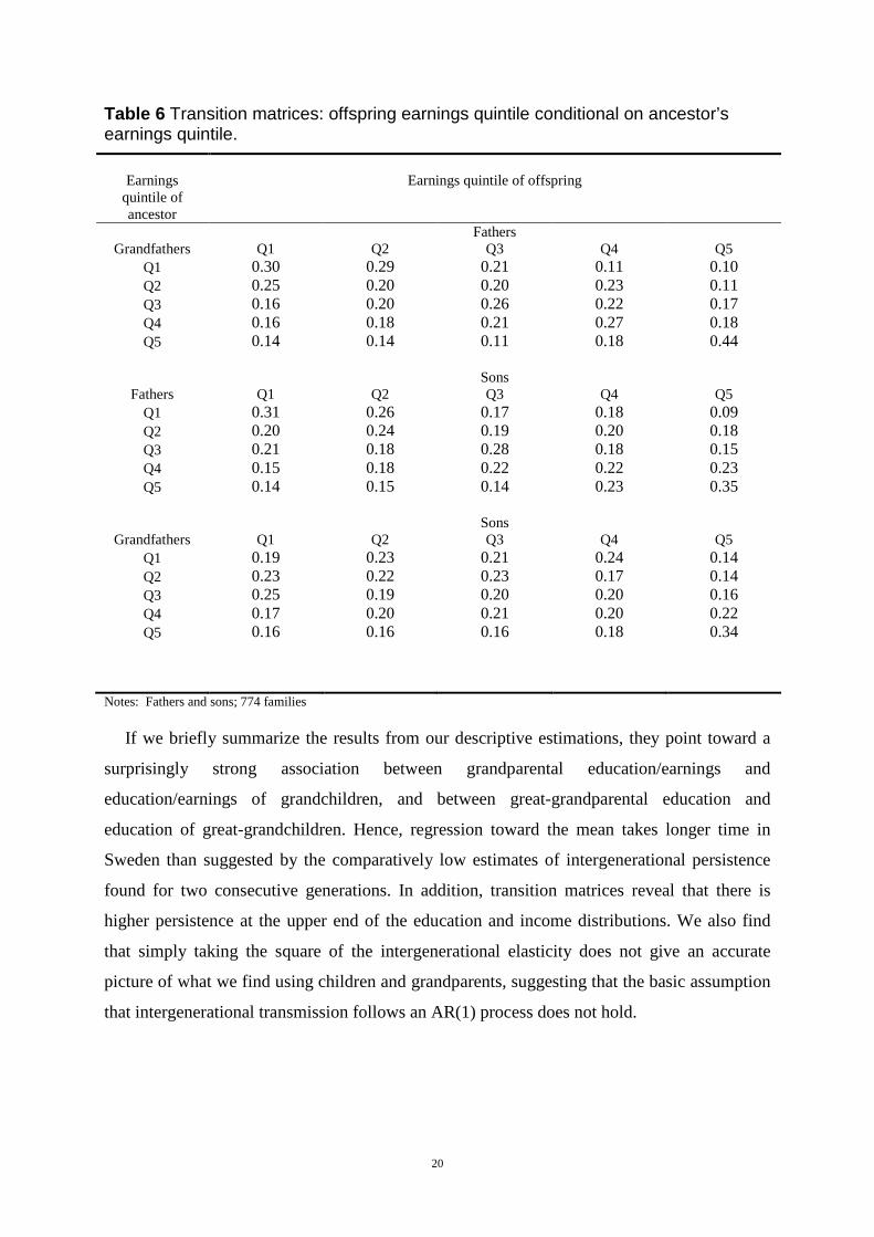
Table 6 shows transition matrices for income quintiles across generations. The first panel

reports the transition probabilities between the first and second generations; the second panel

the corresponding figures for the second and third generations; finally, the third panel shows

the transitions between the first and third generations.

There is one result of particular interest revealed in Table 6: the persistence across two

consecutive generations is higher at the higher end of the income distribution. The highest

persistence in all of three panels is found for the fifth quintile, i.e. the top 20 percent of the

earnings distribution. As many as 34 percent of the grandchildren of those in the fifth quintile

remain at the very top of the income distribution. Interestingly, the persistence in this cell is

almost as high when we compare grandfathers and grandsons (first and third generations) as

when the grandsons are instead compared to their fathers (second and third generations).

20

Table 6 Transition matrices: offspring earnings quintile conditional on ancestor’s earnings quintile.

Earnings

quintile of ancestor

Earnings quintile of offspring

Fathers Grandfathers Q1 Q2 Q3 Q4 Q5

Q1 0.30 0.29 0.21 0.11 0.10 Q2 0.25 0.20 0.20 0.23 0.11 Q3 0.16 0.20 0.26 0.22 0.17 Q4 0.16 0.18 0.21 0.27 0.18 Q5 0.14 0.14 0.11 0.18 0.44 Sons

Fathers Q1 Q2 Q3 Q4 Q5 Q1 0.31 0.26 0.17 0.18 0.09 Q2 0.20 0.24 0.19 0.20 0.18 Q3 0.21 0.18 0.28 0.18 0.15 Q4 0.15 0.18 0.22 0.22 0.23 Q5 0.14 0.15 0.14 0.23 0.35 Sons

Grandfathers Q1 Q2 Q3 Q4 Q5 Q1 0.19 0.23 0.21 0.24 0.14 Q2 0.23 0.22 0.23 0.17 0.14 Q3 0.25 0.19 0.20 0.20 0.16 Q4 0.17 0.20 0.21 0.20 0.22 Q5 0.16 0.16 0.16 0.18 0.34

Notes: Fathers and sons; 774 families

If we briefly summarize the results from our descriptive estimations, they point toward a

surprisingly strong association between grandparental education/earnings and

education/earnings of grandchildren, and between great-grandparental education and

education of great-grandchildren. Hence, regression toward the mean takes longer time in

Sweden than suggested by the comparatively low estimates of intergenerational persistence

found for two consecutive generations. In addition, transition matrices reveal that there is

higher persistence at the upper end of the education and income distributions. We also find

that simply taking the square of the intergenerational elasticity does not give an accurate

picture of what we find using children and grandparents, suggesting that the basic assumption

that intergenerational transmission follows an AR(1) process does not hold.

21

4 Estimating the Becker-Tomes model of intergenerational

transmission of human capital

4.1 The model and its predictions

From the Becker‐Tomes (BT) model of intergenerational human capital transmission follows

that the earnings of a child is positively related to the earnings of the parent, the endowment

of the child and an error term referred to as “market luck”. The positive impact of parental

earnings on the earnings of the child can be derived from utility maximization where parents

optimize between own consumption and investment in children’s human capital (as in Becker

and Tomes, 1979) or because of the existence of borrowing constraints (as in Becker and

Tomes, 1986).13

The model can be modified to explicitly describe the relationship for education instead of

earnings.14 This result in a link between schooling for children and parent specified as:

�� = � + !���� + "���� + ��, (3)

i.e., education (s) of the child-generation t is a linear additive function of education in the parental

generation t-1, unobserved endowment or ability (e) and an error term (�) capturing any exogenous

shocks affecting ��. By construction, �� is uncorrelated with ���� and ����. ! is expected to be

positive because of positive returns to parental investments in human capital.

BT also postulates that transmission of endowments from one generation to the next can be

described as an AR(1) process:

�� = � + #���� + $�, (4)

where the random error $� is assumed to be uncorrelated with ����, �� and ����. Note that

endowments include not only genetically determined ability, but also culture and behavioral factors.15

An immediate implication of this model is that a bivariate regression of children’s

education on parent’s education leads to an upward bias in the estimation of !, since those

13 See also Solon for an alternative derivation. 14 See Holmlund, Lindahl and Plug, 2008, Plug and Vijverberg, 2005, and Sauder, 2006. 15 Plug and Vijverberg, 2003 attempts to decompose the endowment transmission, #, into genetic and non-genetic parts using data on adoptees and their rearing parents. They find that 50-70% is genetically transmitted.

22

with higher endowment also have higher education. This implication has received empirical

support in several studies (see e.g. Holmlund, Lindahl and Plug, 2011).16

The BT model as, expressed in equation (3) and (4), does not allow for a direct effect of

grandparents’ education on the education of grandchildren. Grandparents affect the education

of grandchildren only indirectly through the inheritance of endowments. In the presence of

credit constraints, grandparents also influence grandchildren's education through their

investment in the human capital of the parent generation.

We can use (3) and (4) to obtain:17

�� = �% + (! + #)���� − !#���� + "$��� + �� − #����. (5)

The BT model, hence, implies a negative effect of grandparents’ education on children’s

education conditional on parent’s education. The intuition for this negative coefficient on

����, is that high grandparental education, ����, implies low parental endowment, ����, for a

given level of parental education, ����. From (5) it is also clear that an OLS regression of

children’s outcome on parent’s and grandparent’s outcome generates biased estimates: the

coefficient on parent’s education, ! + #, is estimated with a negative bias and the coefficient

on grandparents education, – !#, is estimated with a positive bias. The reason is that a first-

order lagged version of (3) implies that ()$(����, ����) > 0. To get consistent estimates we

therefore need an alternative approach.

The first attempt to estimate equation (5), addressing the endogeneity problem of parental

education, is provided in Behrman and Taubman (1985). Using a sample of descendents of

twins, they first estimate (5) with OLS and find that grandparent’s education is insignificantly

related to grandchildren’s education. Their IV-estimation, using the education of the

grandfather's twin brother as an instrument for father’s education, yields a significantly

positive estimate of the effect of grandparent's education on child outcomes. As a result, they

conclude that they cannot find support for the prediction of the BT model.

A limitation of their study is, however, that the sample is only generalizable to a rather

restrictive population consisting of the offspring of twins, in particular the offspring of white

16 There is also some evidence that a bivariate regression of children’s income on parent’s income gives an overestimate of the causal intergenerational income effect (see Björklund, Lindahl, and Plug, 2006, and Lefgren, Lindquist and Sims, 2011) 17 Equation (5) follows from equation (3) and (4) simply because the latter two equations constitute an AR(1) model with an autocorrelated error term, which can be rewritten as an AR(2) model, where the coefficient on the first lagged variable will be positive and the coefficient on the second lagged variable will be negative. Also, note that for the constant in equation (5) we have that �% = �(1 − #) + "�.

23

male twins who served in the military during WWII. Furthermore, although novel and

creative, the IV approach makes the questionable assumption that the education of a twin has

no impact on educational attainment of the co-twin’s child. This would not hold if the twins,

who are often close to one another as adults, influence each other’s children.

An alternative approach is used in a study by Sauder (2006) on U.K. data. He finds

positive impact of grandparent’s education using OLS, but no effect using IV. The IV

approach exploits i) two distinct schooling reforms that took place in 1947 and 1973 in the

U.K. and ii) mothers’ birth order as instruments for parent’s and grandparent’s education.

However, both instruments are problematic. First, it is difficult to separate cohort effects from

reform effects when a reform, as was the case here, is introduced simultaneously in the whole

country. Second, birth-order may affect post-education outcomes also through other channels

than educational attainment, as is found in Black, Devereux and Salvanes (2005).

Our approach, suggested already by Becker and Tomes, is to use great-grandparents

education as an instrument for parent’s education, in a regression of children’s education on

parent’s and grandparent’s education. The identifying assumption is that great-grandparent’s

education has no impact on great-grandchildren’s education, over and above the impact

through parent’s and grandparent’s education. This assumption necessarily holds in the simple

Becker-Tomes model as expressed above. Since we have access to four generations of data

for education, we can implement this strategy here.

4.2 Empirical test

Table 7 shows the results from regression of education of a child on the education of parents

and grandparents. The first two columns show results for years of schooling as outcome

variable and the last two columns show results for the probability of graduating from an

academic high-school track. Columns 1 and 3 show results from OLS-regressions and

columns 2 and 4 the IV-results. The lower panel of Table 7 shows the first stage results

corresponding to the IV-estimates.

The results from both first stage regressions are highly significant and the F-statistics for

education of great-grandparents is 30.9 in column 2 and 47.9 in column 4. This suggests that

we have strong instruments. Moving to the IV-estimates, we find that they are positive and

not significantly different from the corresponding OLS-estimates.18 Since a 95 percent

18 We have also checked for non-linear effects of schooling of ancestors in the OLS and IV regressions, but quadratic terms are never statistically different from zero.

24

confidence interval covers a negative value of grandparents’ education, we cannot reject the

Becker-Tomes prediction of a negative coefficient.

25

Table 7 OLS and IV regressions of children’s education on parent’s and grandparent’s education

Years of Schooling Academic high-school track OLS IV OLS IV

Main equation: Education of child Schooling of parent 0.264***

(0.023) [0.368]

0.234 (0.196) [0.327]

0.060*** (0.004) [0.311]

0.045 (0.038) [0.236]

Schooling of grandparent 0.060***

(0.021) [0.092]

0.068 (0.057) [0.105]

0.011*** (0.004) [0.061]

0.015 (0.011) [0.085]

Cluster 673 673 901 901 N 1,823 1,823 2,999 2,999 R2 0.194 0.194 0.126 0.122 First stage equation: Schooling of parent Schooling of grandparent 0.241***

(0.023) [0.268]

0.236*** (0.017) [0.263]

Schooling of great-grandparent

0.224*** (0.040) [0.137]

0.203*** (0.029) [0.124]

Cluster 673 901 N 1,823 2,999 R2 0.177 0.220

Notes: standard errors are clustered at the family.

From the point estimates of the influence of parents and grandparents reported in Table 7,

we get that either ! or #, but not both, is greater than zero. As there is abundant and

convincing evidence that genetic traits are positively transmitted across generations, we

assume that the endowment transmission coefficient # is greater than zero. This would imply

that !, the causal effect of parent’s education on the education of the child, is negative. In

fact, using the estimates in column 2 of Table 7, ! + #=0.234 and –!#=0.068 we can solve

for ! and #. This gives ! =-0.169 and #=0.403.

These estimates are, however, fairly imprecise and in order to investigate how large a

positive value of ! that we can exclude with reasonable statistical confidence we use the delta

method to obtain standard errors. Assuming independence of estimates of ! and #, we get that

26

the standard error for the estimate of ! is 0.127.19 Hence, a 95% confidence interval around

our estimated ! would reject that the causal effect of parental education on the education of

the child is larger than 0.08.

This back of the envelope calculation suggests an estimate much smaller in magnitude than

typical OLS-estimates, including the estimate of 0.296 reported in Table 2 of this paper, but

more in line with recent estimates of the causal effect of education based on outcomes from

compulsory school reforms, twins and adoption data (see Holmlund, Lindahl and Plug, 2011,

for an overview).20

5 Conclusions

We have explored intergenerational transmission of economic status across adjacent and

distant generations over the span of a century. Our data enable us to link great-grandparents

born at the end of the nineteenth century to great-grandchildren who finished their education

in the early twenty-first century. We estimate intergenerational correlations in educational

attainments between these generations and income correlations between the first generation

and their grandchildren. We use the well-known Becker-Tomes model on intergenerational

transmission of human capital to estimate the causal effect of parental education on child

outcomes, using educational attainments of the first generation as an instrumental variable.

We find striking persistence in economic outcomes across generations. There is significant

correlation between the educational attainments of the first generation and their great-

grandchildren. This is also true for the intergenerational earnings correlation. Individuals in

the highest earnings quintile are more than twice as likely to have grandchildren in the highest

income quintile as the rest of the population. From the estimates of the intergenerational

correlations in both educational attainments and earnings we can reject the validity of simple

extrapolations from correlations between adjacent generations to more distant generations as

suggested in elementary text books on labor economics, such as Borjas (2009). Our findings

imply that the persistence of inequality across generations is stronger than we would expect

from the numerous studies on mobility in earnings and educational attainments based on only

19The standard error for the estimate of !, ./, is obtained by solving the two-equation system ./

�+.0�=0.1962

and #�./�+(−!)�.0

�=0.0572. 20 Some might argue that the most convincing evidence of intergenerational education effects comes from rolled out compulsory schooling reforms. Evidence for both Norway (Black, Devereux, and Salvanes, 2005b) and Sweden (Holmlund, Lindahl and Plug, 2011) suggest small local average treatment effects. An exception is Oreopoulos, Page and Huff Stevens (2003) who find large effects on the grade-repetition of children.

27

two generations. We therefore conclude that intergenerational mean reversion takes longer

time than we previously knew from numerous two-generation studies.

In the final part of the empirical analysis, we use the Becker-Tomes model to estimate the

causal effect of parental education on the educational attainments of their children. Based on

our results we cannot reject absence of a causal relation. This result suggests that

intergenerational persistence in economic outcomes, which we found to be stronger than

expected from previous two-generation studies, is generated in some other way. Aspects of

family that are not measured in the data – such as genetic factors, family traditions and social

networks – are possible candidates.

28

References Aaberge, R., M. Mogstad and V. Peragine (2010), “Measuring Long-term Inequality of

Opportunity”, Journal of Public Economics 95, 193-204.

Becker, G. S. and N. Tomes (1979), “An Equilibrium Theory of the Distribution of Income and Intergenerational Mobility”, Journal of Political Economy 87(6), 1153-89.

Becker, G. S. and N. Tomes (1986), “Human Capital and the Rise and Fall of Families” Journal of Labor Economics 4(3), S1-39.

Becker, G. S., K. M. Murphy, and R. Tamura (1990), “Human Capital, Fertility, and Economic Growth”, Journal of Political Economy 98(5), S12-37.

Behrman, J. R. and P. Taubman (1985), “Intergenerational Earnings Mobility in the US and a Test of Becker’s Intergenerational Endowments Model”, Review of Economics and Statistics 67, 144-151.

Bentzel, R. (1952), Inkomstfördelningen i Sverige [The Income Distribution in Sweden], Stockholm: IUI.

Bisin A. and T. Verdier (2000), “Beyond the Melting Pot: Cultural Transmission, Marriage and the Evolution of Ethnic and Religious Traits”, Quarterly Journal of Economics CXV, 955-88.

Björklund, A. and K. G. Salvanes (2011), “Education and Family Background: Mechanisms and Policies”, Handbook in Economics of Education, Amsterdam: Elsevier, 201-247.

Björklund, A., L. Lindahl and M. J. Lindquist (2010), “What More Than Parental Income, Education and Occupation? An Exploration of What Swedish Siblings Get from Their Parents”, The B.E. Journal of Economic Analysis & Policy 10(1), article 102.

Björklund, A., M. Jäntti and R. E. Roemer (2012), “Equality of Opportunity and the Distribution of Long-Run Income in Sweden”, Social Choice and Welfare, forthcoming.

Björklund, A., M. Lindahl and E. Plug (2006), “The Origins of Intergenerational Associations: Lessons from Swedish Adoption Data”, Quarterly Journal of Economics 121(3), 999–1028.

Black S., P. Devereux and K. G. Salvanes, (2005a), “The More the Merrier? The Effect of Family Size and Birth Order on Children’s Education”, Quarterly Journal of Economics 120(2), 669-700.

Black, S. and P. Devereux (2010), “Recent Developments in Intergenerational Mobility”, in O. Ashenfelter and D. Card (eds.), Handbook of Labor Economics, Vol. 4B, Ch. 16, Amsterdam: Elsevier.

Black, S., P. Devereux and K. G. Salvanes (2005b), “Why the Apple Doesn’t Fall Far: Understanding Intergenerational Transmission of Human Capital”, American Economic Review 95(1), 437-449.

29

Böhlmark, A. and M. J. Lindquist (2006), “Life-Cycle Variations in the Association between Current and Lifetime Income: Replication and Extension for Sweden”, Journal of Labor Economics 24(4), 879-900.

Borjas, G. J. (2009), Labor Economics, 5th edition. New York: Irwin/McGraw-Hill.

Diamond, P. A. (1965), “National Debt in a Neoclassical Growth Model”, American Economic Review, 55, 1126–1150.

Galor, O. and J. Zeira (1993), “Income Distribution and Macroeconomics”, Review of Economic Studies 60(1), 35-52.

Haider, S. and G. Solon (2006), “Life-Cycle Variation in the Association between Current and Lifetime Earnings”, American Economic Review 96(4), 1308-1320.

Holmlund, H., M. Lindahl and E. Plug (2008), “The Causal Effect of Parents' Schooling on Children's Schooling: A Comparison of Estimation Methods”, IZA Discussion Paper 3630.

Holmlund, H., M. Lindahl and E. Plug (2011), “The Causal Effect of Parents' Schooling on Children's Schooling: A Comparison of Estimation Methods”, Journal of Economic Literature 49(3), 614-650.

Lee, C. and G. Solon (2009), “Trends in Intergenerational Income Mobility”, Review of Economics and Statistics 91(4), 766-772.

Lefgren, L., M Lindquist, and D. Sims, “"Rich Dad, Smart Dad: Decomposing the Intergenerational Transmission of Income," Mimeo, SOFI, Stockholm University, October 2011.

Maurin, E. (2002), “The Impact of Parental Income on Early Schooling Transitions: A Re-examination Using Data over Three Generations”, Journal of Public Economics 85(3), 301-332.

Mulligan, C. B. (1997), Parental Priorities and Economic Inequality, Chicago: University of Chicago Press.

Oreopoulos, Philip, Marianne Page and Anne Huff Stevens. 2006. “The Intergenerational Effects of Compulsory Schooling.” Journal of Labor Economics, 24(4): 729-760.

Plug, E. and W. Vijverberg (2003), “Schooling, Family Background, and Adoption: Is it

Nature or Is it Nurture”, Journal of Political Economy 111(3), 611--41.

Plug, E. and W. Vijverberg (2005), “Does Family Income Matter for Schooling Outcomes? Using Adoptees as a Natural Experiment”, Economic Journal 115(506), 880-907.

Roemer, J. E. (1993), “A Pragmatic Theory of Responsibility for the Egalitarian Planner”, Philosophy & Public Affairs 22, 146-166.

Sacerdote, B. (2004), “What Happens When We Randomly Assign Children to Families?”, NBER Working Paper No. 10894.

Sacerdote, B. (2005), “Slavery and the Intergenerational Transmission of Human Capital”, Review of Economics and Statistics 87(2), 217-234.

30

Saez-Marti M. and A. Sjögren (2008), “Peers and Culture”, Scandinavian Journal of Economics 110(1), 73-92.

Sauder, U. (2006), “Education Transmission across Three Generations - New Evidence from NCDS Data”, Mimeo, University of Warwick.

Solon, G. (1999), “Intergenerational Mobility in the Labor Market”, in O. Ashenfelter and D. Card (eds.), Handbook of Labor Economics, vol. 3, ch. 29, 1761-1800, Amsterdam: Elsevier.

Warren, J. R. and R. M. Hauser (1997), “Social Stratification across Three Generations: New Evidence from the Wisconsin Longitudinal Survey”, American Sociological Review 62(4), 561–572.

Appendix: Institutional Background

The four generations studied in this paper span a century during which Swedish society was

transformed from early industrialization to present day welfare society. While subsidized

childcare, generous child allowances, free schooling through high school, generous grants and

loans for higher education, social security, unemployment benefits, free health care and

pensions constitute today’s welfare system, Malmö in the beginning of the 20th century had

some, but not all of these institutions in place, when the parents of the initially sampled index

generation grew up.

Malmö is located in the southern part of Sweden. It was and is by population size

Sweden’s third city. At the beginning of the 20th century Malmö grew at a rapid pace and

tripled its population from 61,000 to 192,000 between 1900 and 1950, compared to today’s

300,000. Much of the population growth was a result of rapid urbanization. Malmö was early

on one of the most industrialized cities in Sweden. When the original data collection of the

Malmö study was initiated, in 1938, three large employers dominated.21 After 1960, an

increasing fraction was employed within the public sector and by 1980, 20% of the men and

50% of the women held public sector jobs.

In the early 20th century, Swedish compulsory schooling was only six years, but a seventh

year of was introduced already in 1914 in Malmö. Yet, many children kept leaving school

after six years. Seven years of schooling only become the norm around 1920 when a

municipal grant was introduced to compensate poor families for the lost earnings during the

seventh year of school. This grant existed until 1936 when compulsory schooling was

extended to 7 years throughout Sweden. In the late 1930’s almost a third of all Malmö

21 Kockums, a shipbuilding company and mechanical workshop, with 2,300 employees; Skånska Cement, a construction company, with almost 2,000 employes; and Malmö strumpfabrik, a stocking factory, with more than 1,000 employees.

31

children continued beyond compulsory schooling. School enrolment, was hence higher than

in the rest of Sweden. Malmö was also the first large municipality to extend compulsory

schooling to 9 years in 1962. Arguably, basic educational infrastructure was well developed

and accessible already to the index-generation studied here.

Since the 1920’s, loans to help finance higher education were in principle available to the

tiny fraction of young people qualified to studying at Universities. In the late 1950’s student

loans were also made available for studies at the high school level. The present day generous

grant and loans program for university students was introduced in 1964. Since then, credit

constraints are arguably unlikely to play a role for higher education choices.

Although our sample is not a random sample from the Swedish population, Malmö was

(and is) a fairly representative city in Sweden. This can be seen if we compare the earnings

distribution for our first generation from Malmö (using our sample) with the earnings

distribution for the entire county. To do this we use estimates of the earnings distribution

obtained by Bentzel (1952), who used tax registers to construct measures of the Swedish

income distribution. Figure 2 compares the earnings distribution of the first generation in our

data in 1937 with those obtained by Bentzel for the years 1935 and 1945. It is interesting to

note that the income distribution among the Malmö families does not deviate drastically from

the national income distribution.

32

Figure 2 A comparison of earnings distribution for the first generation in the Malmo

data for 1937 with those obtained by Bentzel (1952) for Sweden in 1935 and 1945.

Source: Own computation based on Malmo data and Bentzel (1952).

0

10

20

30

40

50

60

70

80

90

100

1 2 3 4 5 6 7 8 9 10

Acc

um

ula

ted

in

com

e s

ha

re %

Accumulated income share by decile of the

income distribution

1935 Nation 1937 Malmo 1945 Nation