DI

SC

US

SI

ON

P

AP

ER

S

ER

IE

S

Forschungsinstitut zur Zukunft der ArbeitInstitute for the Study of Labor

Personality, IQ, and Lifetime Earnings

IZA DP No. 8235

June 2014

Miriam Gensowski

Personality, IQ, and Lifetime Earnings

Miriam Gensowski University of Copenhagen

and IZA

Discussion Paper No. 8235 June 2014

IZA

P.O. Box 7240 53072 Bonn

Germany

Phone: +49-228-3894-0 Fax: +49-228-3894-180

E-mail: iza@iza.org

Any opinions expressed here are those of the author(s) and not those of IZA. Research published in this series may include views on policy, but the institute itself takes no institutional policy positions. The IZA research network is committed to the IZA Guiding Principles of Research Integrity. The Institute for the Study of Labor (IZA) in Bonn is a local and virtual international research center and a place of communication between science, politics and business. IZA is an independent nonprofit organization supported by Deutsche Post Foundation. The center is associated with the University of Bonn and offers a stimulating research environment through its international network, workshops and conferences, data service, project support, research visits and doctoral program. IZA engages in (i) original and internationally competitive research in all fields of labor economics, (ii) development of policy concepts, and (iii) dissemination of research results and concepts to the interested public. IZA Discussion Papers often represent preliminary work and are circulated to encourage discussion. Citation of such a paper should account for its provisional character. A revised version may be available directly from the author.

IZA Discussion Paper No. 8235 June 2014

ABSTRACT

Personality, IQ, and Lifetime Earnings* Talented individuals are seen as drivers of long-term growth, but how do they realize their full potential? In this paper, I show that even in a group of high-IQ men and women, lifetime earnings are substantially influenced by their education and personality traits. I identify a previously undocumented interaction between education and traits in earnings generation, which results in important heterogeneity of the net present value of education. Personality traits directly affect men’s earnings, with effects only developing fully after age 30. These effects play a much larger role for the earnings of more educated men. Personality and IQ also influence earnings indirectly through educational choice. Surprisingly, education and personality skills do not always raise the family earnings of women in this cohort, as women with very high education and IQ are less likely to marry, and thus have less income through their husbands. To identify personality traits, I use a factor model that also serves to correct for prediction error bias, which is often ignored in the literature. This paper complements the literature on investments in education and personality traits by showing that they also have potentially high returns at the high end of the ability distribution. JEL Classification: J24, I24, J16 Keywords: personality traits, social skills, cognitive skills, returns to education,

life-time earnings, Big Five, human capital, factor analysis Corresponding author: Miriam Gensowski Department of Economics University of Copenhagen Øster Farimagsgade 5 Office 26.2.39 1353 Copenhagen K Denmark E-mail: Miriam.Gensowski@econ.ku.dk

* I am deeply grateful to James J. Heckman, Steven N. Durlauf, and Gary S. Becker for their continued support of this research, which was produced during my time at the University of Chicago. Peter Savelyev greatly facilitated my work with the Terman data by generously sharing his experience and detailed knowledge of the survey, and Min Ju Lee and Molly Schnell provided outstanding research assistance in data preparation. I would like to thank everyone who provided helpful feedback, individually or during presentations, especially Mathilde Almlund, Katarína Borovičková, Deborah Cobb-Clark, Philipp Eisenhauer, Rémi Piatek, Pia Pinger, Stefanie Schurer, Jeffrey Smith, and Lucas Threinen. A Web Appendix with additional material and a description of the data can be found at http://www.econ.ku.dk/gensowski/research/Terman/TermanApp.pdf.

1 Introduction

Talented individuals are seen as drivers of long-term growth (Hughes, 1986; Jones, 2011;

Murphy et al., 1991). But it is not clear why some highly talented individuals realize their

potential and others do not. For example, one would expect individuals with IQs above 140,

who are in the top 0.5% of the ability distribution, to excel in life, to be over-achievers and to

contribute to society by the sheer power of their talent. In a cohort study that follows men

and women of this promise, however, we see that while many of them fulfil this expectation,

their life outcomes and earnings vary greatly. This paper argues that a substantial amount

of this variation can be attributed to differences in education and personality traits. The

data for this analysis followed high-ability men and women over their lifetimes, and is called

the Terman study.1

While a growing literature documents effects of personality traits on earnings, these stud-

ies are typically limited to cross-sectional observations, point-in-time measures, or longitudi-

nal datasets with few years of follow-up. Many datasets contain only one or two measures of

personality, whereas the Terman study provides measures that map into the well-established

comprehensive taxonomy of the Big Five (McCrae and John, 1992). Using the full life-cycle

earnings data of the Terman study, I show how personality traits affect earnings differently

over the course of a working life. The direct effects of personality traits on earnings are not

detectable in the early years of a career—they only develop fully later in a person’s work-

ing life (after age 30). Furthermore, these effects vary across education levels. Men with

post-graduate education benefit from traits such as Conscientiousness or Extraversion more

than twice as much than men with a bachelor’s degree or less. Most of the existing studies

do not allow for this trait-education interaction, and therefore over- or under-estimate the

direct effects of personality traits.

Ignoring this heterogeneity is particularly consequential for women. Women might benefit

from a given trait if they hold at most a bachelor’s degree, but suffer from the same trait

when they hold a master’s degree or more.

I also analyze how women’s family earnings, as opposed to just their own earnings,

are differentially affected by personality traits and IQ.2 Only about half of the women of

this cohort are securely attached to the labor force, and many women rely on husbands as

bread-winners. Own earnings and husband’s earnings react differently to personality traits.

1The American psychologist Lewis Terman initiated this study with boys and girls born around 1910.It is the longest prospective cohort study in existence (Friedman et al., 1995a), and is described in Terman(1925, 1926, 1930, 1947, 1959).

2To obtain family earnings, the full length of the earnings data is supplemented with complete marriagehistories, and the corresponding husband’s earnings.

1

Conscientiousness, for example, increases own earnings and decreases spousal earnings for

highly educated women.

The finding of strong influences of personality traits on lifetime earnings complements

the literature on early childhood interventions, or other programs with a focus on social

skill-building activities. Most of these are targeted at disadvantaged, and sometimes low-

IQ, populations (examples are Grossman and Tierney, 1998; Heckman et al., 2010, 2013;

University of Chicago Crime Lab, 2012). These interventions’ attractiveness lies in the

greater malleability of social skills than “hard skills” or IQ, which is generally thought fixed

after age 10. It is not clear from the literature, however, whether high-IQ children would

also benefit from improving these social skills, or whether their life outcomes would even be

altered. I show that social skills matter, at least for men, to orders of magnitude that are

about half of the impact of education.

I further establish that the effects of intelligence on earnings are still positive even at very

high levels of IQ for men. This is not only due to higher educational attainment but also to

a direct impact of ability on earnings. For women, in contrast, having a higher IQ results in

lower lifetime earnings if they are at the top of the educational attainment spectrum.

Personality traits and IQ also have an indirect effect on lifetime earnings, through ed-

ucational attainment. They might increase the level of education achieved, and thus also

increase earnings through positive rates of return to education. In order to identify the rate

of return to education, I estimate the causal effect of education on earnings through match-

ing on personality traits, as well as a rich set of background variables that are available in

the Terman data. This technique does not rely on instruments and addresses “ability bias”

by explicitly accounting for cognitive and “non-cognitive” ability. In computing the internal

rates of return, this paper fills in two gaps in the literature on returns to schooling.

First, it bypasses the ad hoc methods widely used to approximate the rate of return from

cross sections of data (Mincer, 1974). By using lifetime earnings histories, it presents ex-post

estimates of the internal rate of return to schooling. For most pairwise comparisons, the

return is substantial. For example, a bachelor’s degree over high school diploma yields a

return of 12.5% for men. A standard Mincer regression with years of schooling produces

estimates that are very different from pairwise returns.

Second, this paper explores the rate of return to education for highly able students.

Researchers are interested in contrasting rates of return for the “average student” with

the “valedictorian.” In representative datasets, the number of observations of these high-IQ

individuals is so small that any statement about returns at the high end would be unreliable.

With the fairly large number of individuals in the Terman study (total of 1528), I can

establish that even at the high end of the cognitive spectrum, education has positive returns.

2

A simple comparison with the 1950 census shows that the average earnings difference between

men with a bachelor’s versus high school degree is slightly higher for the Terman men than

the average man (11.4% versus 10.7%). But when the Terman men’s earnings are top coded

as they would have been in the census, their earnings difference decreases to 8.6%.

The cohort studied here was born in the early years of the last century, when women had a

fundamentally different role in the labor market and society than women do today (Goldin,

1992). The marriage market determined whether these women benefited from education,

or if instead they decreased their family earnings by obtaining post-graduate education. In

terms of own earnings, women had low rates of return to education up to a bachelor’s degree.

Less educated women were unlikely to work, and their skills and education only marginally

affected their own earnings. Women with postgraduate degrees, however, saw earnings gains

that were similar to men’s in terms of signs and relative magnitudes.

But education differentially affected family earnings, which are the sum of own earnings

and any husband’s earnings (which were zero if no husband was present). On the one hand,

education increased spousal earnings through assortative mating—the correlation between

the spouses’ years of education is 0.36 in the Terman sample. Seventy percent of Terman

females with a bachelor’s degree married men with a bachelor’s degree or more, who had

accordingly higher earnings.3 On the other hand, the most highly educated women were

much less likely to be married. This lower propensity to marry represents an additional cost

to post-graduate education for women of this cohort.

The paper proceeds in the following way. Section 2 discusses the rich data analyzed in

this paper. Section 3 decomposes the effects of psychological traits on total lifetime earnings

into the direct and indirect channels. Section 4 breaks down the direct effects by education,

and shows results by age. The educational sorting is discussed in Section 5, and the rate of

return to education in Section 6. Section 7 concludes.

2 The Terman Survey

The analysis in this paper is based on a survey initiated by the prominent psychologist

Lewis Terman to study the life outcomes of high IQ children. The criterion for inclusion

in the sample was having a Stanford-Binet IQ score of 140 or higher, which corresponds

to approximately 0.5% of the population. These high IQ children were identified through

a procedure that canvassed all school grades 1-8 in California in 1921-1922. The Terman

sample consists of 856 boys and 672 girls, born around 1910. The cohort was followed until

3The comparable number in the 1940 census is 56-60% (and increases over time), as reported in Mare(1991) and Pencavel (1998).

3

1991, with surveys every 5–10 years.4 It is the longest prospective cohort study that also

has data on earnings.

The Terman data has rich information about its participants. Information is available

on their IQs, their personality traits, their early and current health, their background and

conditions when growing up, and other aspects of their lives, including marriage, children,

and other life events.5 The educational status and attainment data as well as earnings data

is very detailed, allowing me to construct trajectories by age.

The Terman data have been used extensively by psychologists to study health and

longevity outcomes in relation to the personality trait of Conscientiousness and parental

divorce or marriage.6 Only a few economists have worked with the data, and they mainly

analyzed family outcomes such as marriage, divorce, or fertility (Becker et al., 1977; Michael,

1976; Tomes, 1981). The Terman retirement behavior is analyzed by Hamermesh (1984),

and Savelyev (2012) investigates the effects of education and Conscientiousness on longevity.

Earnings outcomes were only studied by Leibowitz (1974), but she did not exploit the lon-

gitudinal feature of the data.

Earnings Histories. I construct a full lifetime earnings history, as well as education and

marriage profiles, for each participant. The earnings measures for computing the rates of

return to schooling are annual earnings after tuition, in 2010 U.S. Dollars.7 Tuition costs

are estimated from data on tuition rates at each of the colleges or universities attended by

the Terman participants. Tuition is subtracted from earnings at each year that college is

attended, at both the undergraduate and graduate level. For inactive workers, as well as for

the deceased, earnings are zero. Full life cycle profiles can thus include zeros. Except where

specified, all estimations use earnings that are truncated at the 97th percentile, so that the

observed effects are not driven by extreme earnings values.

4Its attrition rate is less than 10%. Those who dropped out do not differ in terms of income, education,and demographic factors (Sears, 1984), or psychological measures (Friedman et al., 1993).

5All survey items are listed in the codebooks Terman and Sears (2002a); Terman et al. (2002a) andTerman and Sears (2002b); Terman et al. (2002b).

6Friedman (2000, 2008); Friedman and Martin (2011); Friedman et al. (1995b, 1993); Martin et al. (2007,2002) and Martin et al. (2005); Tucker et al. (1997, 1996, 1999).

7Web Appendix A, found at http://www.econ.ku.dk/ gensowski/research/Terman/TermanApp.pdf., de-scribes how the earnings profiles were constructed and specifies how tax rates or tuition costs are obtained.The estimations in Section 4 and Section 6 are on pre-tax earnings. For comparability with papers suchas Becker (1964) and Heckman et al. (2006), Web Appendix Section C.4 shows all corresponding figuresand tables for after-tax earnings. Tax rates there reflect the marital status obtained from the Terman mar-ital histories. Section C.5 presents alternative tuition imputations. The price series used for all inflationadjustments is the CPI.

4

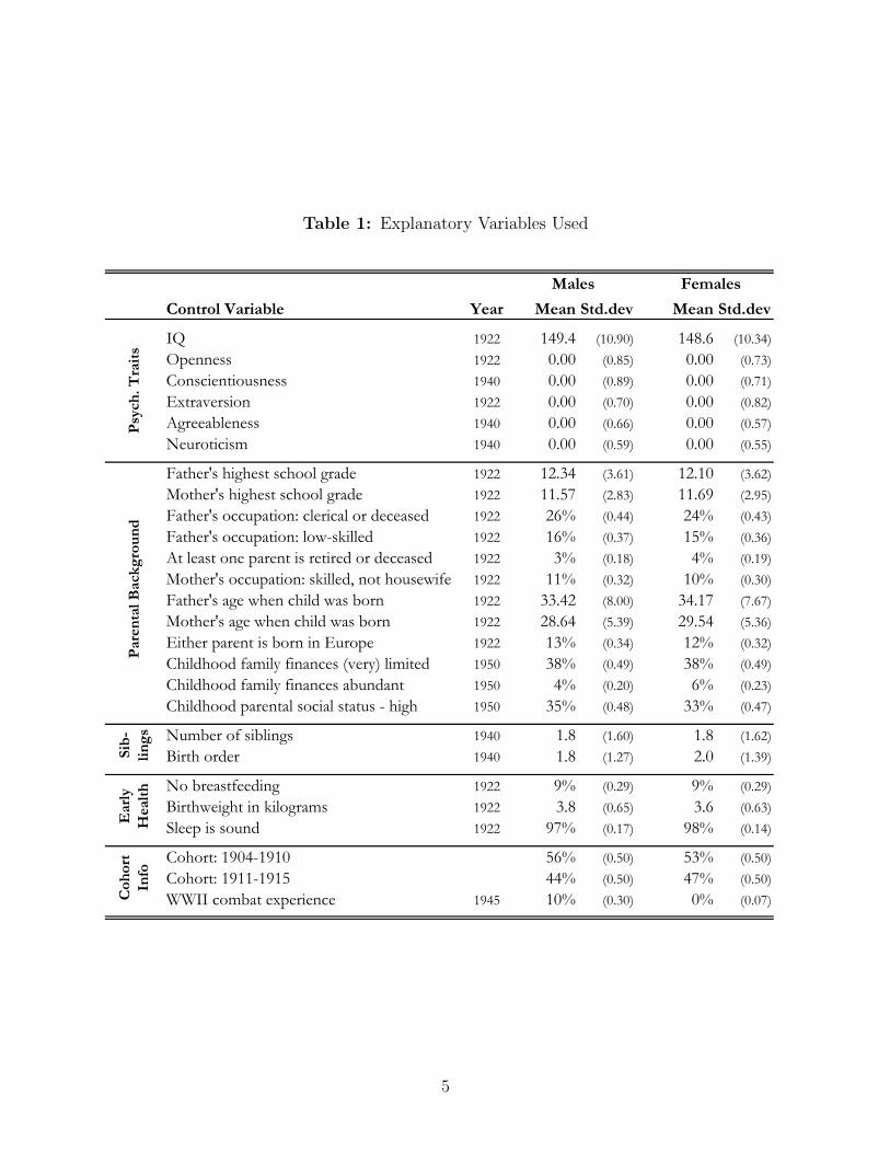
Table 1: Explanatory Variables Used

Control Variable Year Mean Std.dev Mean Std.dev

IQ 1922 149.4 (10.90) 148.6 (10.34)

Openness 1922 0.00 (0.85) 0.00 (0.73)

Conscientiousness 1940 0.00 (0.89) 0.00 (0.71)

Extraversion 1922 0.00 (0.70) 0.00 (0.82)

Agreeableness 1940 0.00 (0.66) 0.00 (0.57)

Neuroticism 1940 0.00 (0.59) 0.00 (0.55)

Father's highest school grade 1922 12.34 (3.61) 12.10 (3.62)

Mother's highest school grade 1922 11.57 (2.83) 11.69 (2.95)

Father's occupation: clerical or deceased 1922 26% (0.44) 24% (0.43)

Father's occupation: low-skilled 1922 16% (0.37) 15% (0.36)

At least one parent is retired or deceased 1922 3% (0.18) 4% (0.19)

Mother's occupation: skilled, not housewife 1922 11% (0.32) 10% (0.30)

Father's age when child was born 1922 33.42 (8.00) 34.17 (7.67)

Mother's age when child was born 1922 28.64 (5.39) 29.54 (5.36)

Either parent is born in Europe 1922 13% (0.34) 12% (0.32)

Childhood family finances (very) limited 1950 38% (0.49) 38% (0.49)

Childhood family finances abundant 1950 4% (0.20) 6% (0.23)

Childhood parental social status - high 1950 35% (0.48) 33% (0.47)

Number of siblings 1940 1.8 (1.60) 1.8 (1.62)

Birth order 1940 1.8 (1.27) 2.0 (1.39)

No breastfeeding 1922 9% (0.29) 9% (0.29)

Birthweight in kilograms 1922 3.8 (0.65) 3.6 (0.63)

Sleep is sound 1922 97% (0.17) 98% (0.14)

Cohort: 1904-1910 56% (0.50) 53% (0.50)

Cohort: 1911-1915 44% (0.50) 47% (0.50)

WWII combat experience 1945 10% (0.30) 0% (0.07)

FemalesMales

Ear

ly

Hea

lth

Coh

ort

Info

Psy

ch. T

rait

sP

aren

tal B

ackg

rou

nd

Sib-

ling

s

5

IQ and Personality Measures in the Terman Sample. IQ is measured at study entry

in 1922. The personality traits collected in this early survey are remarkably similar to the

modern Big Five taxonomy, even though the measures were collected some 70 years before

the Big Five were codified.8 The dedicated items for each personality factor were determined

with exploratory factor analysis. Web Appendix Section B.2 provides details on the measures

and the factor analysis that operationalizes the traits.

Openness and Extraversion are measured in 1922 by ratings from teachers and parents

(taking the average). Extraversion is indicated by the subject’s “fondness for large groups,”

“leadership,” and “popularity with other children”, and Openness is extracted from ratings

of the subject’s “desire to know,” “originality,” and “intelligence.”9 The other three traits

Conscientiousness, Agreeableness, and Neuroticism are based on self-ratings in 1940. The

dedicated items for each are either from a personality inventory,10 where questions about

usual behavior and feelings can be answered “yes,” “no,” and “?,” or self-ratings of per-

sonality traits on an 11-point scale. Examples of Conscientiousness items are self-ratings of

“How persistent are you in the accomplishment of your ends?” or “In your work do you

usually drive yourself steadily?”, and an example of an Agreeableness item is “In general,

how easy are you to get on with?”. Neuroticism is based on questions such as “Are you

moody?”. The reverse of Neuroticism is called Emotional Stability.

The personality traits are summarized by factor scores (Joreskog and Sorbom, 1979;

Mulaik, 2010; Thurstone, 1935). Factor scores are predicted using the estimates of a standard

linear factor model, using the Bartlett method (Bartlett, 1937; Thomson, 1938). These

factors scores will then be used in the regressions.

Even though the Terman survey is very selective in terms of IQ, it is not selective in terms

of personality, as Martin and Friedman (2000) show. Generally, personality traits correlate

only weakly with IQ (see Dauber and Benbow, 1990; Eysenck, 1993). The only trait that is

moderately positively correlated with IQ is Openness to experience. In the Terman sample,

the correlation coefficient is r = 0.2.

8See Goldberg (1993). The Big Five traits are Openness, Conscientiousness, Extraversion, Agreeableness,and Neuroticism (OCEAN). While the traits from the Terman data are conceptually very close to the BigFive personality traits, they are not measured using the same inventory. Martin and Friedman (2000)have established that the personality factors based on the Terman questionnaires correspond closely to theanalogous Big Five traits, as measured by the NEO PI-R: The correlations are high.

9Since “intelligence” is a facet of Openness, it might seem as if Openness and IQ measure the sameunderlying trait (see the discussion in Almlund et al., 2011). Note that the IQ test is a direct measureof the subject’s cognitive ability, while the parents’ and teachers’ ratings describe their impressions of thechild. Furthermore, several measurements of these impressions combine to generate the factor defined bypsychologists as “Openness.” Hogan and Hogan (2007) define Openness as the degree to which a personneeds intellectual stimulation, change, and variety.

10The Bernreuter scale is described in Terman et al. (2002a).

6

Education and Background Variables. The covariates that are used as control vari-

ables include father’s and mother’s background information (education, occupation, social

status, region of origin, age at birth of subject), family environment (family’s finances when

growing up, number of siblings, birth order), and early childhood health (birthweight, breast-

feeding, sleep quality in 1922). Descriptive statistics of these variables are given in Table 1.

Sample. The sample used to conduct the analysis does not include the youngest and oldest

participants, since their selection into the sample was non-standard.11 Only respondents

with valid education information are included. Non-Caucasian children and those with rare

genetic diseases are excluded. In order to have full earnings histories from age 18 to 75, only

individuals with 10 or fewer years of missing earnings information are retained in the sample.

Individuals lacking all personality information are excluded. The few individuals who lack

only a subset of items remain in the sample, as long as at least two traits are observed.

Regressions are then augmented with a multiple imputation routine to impute the missing

values on the basis of the observed traits. The full estimation sample thus consists of 595

men and 422 women.

3 Effects of Psychological Traits on Lifetime Earnings

IQ and personality traits influence the lifetime earnings of men and women in the Terman

sample. Over a lifetime, how much more will more conscientious men earn? Scoring one

standard deviation higher will lead to about 18% higher lifetime earnings. But different

channels might be responsible for this effect. Personality traits could influence wages di-

rectly in the marketplace, through pricing of the traits in a hedonic model. Alternatively,

it is known that personality traits influence educational attainment—if there is a positive

return to education, traits might thus have an indirect effect on lifetime earnings through

educational attainment. This section estimates the total marginal effects of traits on the

sum of lifetime earnings and decomposes them into direct and indirect effects.

3.1 Estimation Procedure

All effects of education and personality traits on earnings are identified using a “selection

on observables” or “matching” assumption (Heckman and Robb, 1985), based on a full set

11While most students were identified through the canvassing of schools, a few other students were includedin the sample because the researchers were made aware of these intelligent children through other means—forexample, by their siblings (Terman, 1925). It is standard practice to exclude them. See Web Appendix A.6for a detailed description of the estimation sample and how it differs from the complete Terman sample.

7

of covariates. The exact link to the standard Roy model of counterfactuals is presented

in Section B.1. The specific implementation of this assumption here is Ordinary Least

Squares,12 as in the following estimation with a linear specification for earnings at age t:

Yt = θJ∑j=1

δj,tDj +J∑j=1

κj,tDj +Xtβt + ρt t = 1, . . . , T ; j = 1, . . . , J. (1)

θ is a vector of traits (IQ and personality factors), δj,t the corresponding vector of coefficients

by schooling level j, and Dj an indicator matrix of the same dimension as δj,t. κt,j is the

average treatment effect of schooling level j, or the causal effect of schooling given the

matching assumption. Xt is a vector of background variables with coefficients βt, and ρt is

a mean-zero error term. Equation (1) is estimated separately for men and women.

Since the factor scores for personality traits are estimated on the basis of factor model

estimates, their predicted values contain prediction uncertainty and the variance of these

scores is higher than of the true factors. Simply including factor scores in a least squares

regression leads to attenuation bias in the coefficients. This bias is usually ignored by

economists using predicted factor scores, which might explain frequent insignificant effects

of these factor scores. In this paper, I correct for this estimation error with the method

described by Croon (2002). This method was developed for the simple model where factor

scores enter in levels only. Thus, the bias correction has to be expanded to account for the

interaction terms between the predicted factor scores and education in Eq. (1). Section B.3

in the Appendix provides the details of this adjustment is performed. It is standard practice

to bootstrap the standard errors or estimate them with other Monte Carlo methods (Bolck

et al., 2004), because regular standard errors do not take account of the prediction variance

and the fact that the measurement system is estimated. All standard errors presented are

bootstrapped non-parametrically and all estimates, unless otherwise noted, condition on

personality traits (using extracted factors), IQ and family background variables.

As described in Section 2, the measures of personality traits are obtained when the Ter-

man participants were around 12 - 30 years old. While levels of psychological traits change

systematically with maturation, personality throughout adulthood is very stable over time

in terms of rank order. As numerous studies have shown, the rank order correlation of traits

within one person over very long time spans is remarkably high,13 and even from adolescence

to adulthood there is “more stability than change” (Roberts et al., 2001). Judge et al. (1999)

12The results presented here do not depend on the assumption of linearity — other models, includinga nonparametric one, yield the same effects of education on earnings. The description of these, and acomparison of the results, is in Web Appendix Section C.8.

13See Costa and McCrae (1994); Leon et al. (1979); Roberts and DelVecchio (2000); Roberts et al. (2006);Robins et al. (2001).

8

show that the correlations of Big Five traits with adult income and occupational status are

practically identical between childhood personality measures and measures taken in adult-

hood. Thus, the present identification of effects of personality traits relies on the assumption

that the rank in traits which are measured relatively early in the Terman participants’ lives

are representative of what their rank will be later on. At the same time, this stability does

not extend to childhood. On the contrary, personality has been shown to be more malleable

than IQ throughout childhood. In this sense, this paper exploits the duality of changeability

and stability of traits at the same time.

As a first overview, the effects of personality traits on total lifetime earnings, defined

as Y Ti =

∑75t=18 Yit, are analyzed. (The Web Appendix presents corresponding results for

discounted lifetime earnings.) Based on an equation similar to Eq. (1), define conditional

average lifetime earnings as

E[Y T |θ,Xt

]= θ

J∑j=1

δj,TE [Dj|θ,X] +J∑j=1

κj,TE [Dj|θ,X] +XβT (2)

3.2 Decomposing the Effect of Personality and IQ on Total Life-

time Earnings

The marginal average effect of trait θk can be decomposed into a direct effect and two indirect

effects:

∂E[Y T |θ,Xt

]∂θk

=J∑j=1

δk,j,TE [Dj|θ,X]︸ ︷︷ ︸direct

+ θJ∑j=1

δj,T∂E [Dj|θ,X]

∂θk︸ ︷︷ ︸indirect(alt.direct)

+J∑j=1

κj,T∂E [Dj|θ,X]

∂θk︸ ︷︷ ︸indirect(education)

(3)

Here, δk,j,T is the entry corresponding to trait θk in the vector δj,T . The magnitude of the

direct effect of traits depends on educational attainment, since the specification in (1) allows

for heterogeneous effects. The indirect effects both arise because trait θk alters educational

attainment. At a different educational attainment, the direct effects of all personality traits

are altered (indirect(alt.direct)), and naturally there is a different return to education (indi-

rect(education)). Educational choice, and thus E [Dj|θ,X], is estimated with a generalized

ordered logit model (see also the results in Section 5).

Figure 1 presents the decomposition of these marginal effects of personality and IQ on

total lifetime earnings of men and women in the Terman sample. Personality traits and IQ

clearly play a large role in determining lifetime earnings of males (first row). Ceteris paribus,

lifetime earnings are higher if the men are more conscientious and extraverted, and if they

9

Figure 1: Decomposition of Marginal Effects of Psychological Traits on Lifetime Earnings

Own Earnings, Men

Own Earnings, Women

Family Earnings, Women

−250

0

250

500

750

−250

0

250

500

750

−250

0

250

500

750

Openn. Consc. Extrav. Agree. Neurot. IQ

Effe

cts

in 1

000

US

D (

2010

)

Indirect Effect through Education Direct Effect of Trait

Notes: Stacked marginal effects showing how much an increase of one standard deviation in each personality

trait influences total lifetime earnings (results from estimation Eq. (3), evaluated at mean values of all

covariates and personality traits). Total lifetime earnings are the sum of earnings in thousand US Dollars

from age 18 to 75, after tuition. One indirect effect is not shown, indirect(alt.direct) in Eq. (3), because the

traits are centered around zero, making this particular indirect effect zero as well.

10

are less agreeable. The combined effect of Conscientiousness, at around $750,000, means that

a man with one standard deviation higher Conscientiousness will have about 22% higher net

lifetime earnings than his otherwise equal peer. Lifetime earnings are also increasing in IQ.

The decomposition reveals two facts. First, the direct effect of traits on earnings out-

weighs the indirect effects through education. This implies that researchers who find associ-

ations between traits and earnings should focus on interpretations that relate traits directly

to earnings rather than to education. It also raises the question of why the indirect effects

are relatively smaller. It might be because the marginal effects of the traits on educational

attainment are small, or because returns to schooling are small. Sections 5 and 6 will show

that the returns to schooling are substantial, but that some traits have a limited influence

on educational attainment. Second, direct and indirect effects do not have to be of the

same sign. As demonstrated by Openness to experience, personality traits that increase

educational attainment might not be rewarded in the marketplace directly.

Women’s own lifetime earnings (second row) are affected differentially by traits — the

effects are much smaller and not even of the same sign as for men. The family earnings

of women (third row) are only meaningfully related to Conscientiousness and Extraversion,

which have positive direct effects. Generally, the effects of personality traits on life-time

earnings are much smaller for women, even accounting for their spousal earnings.

4 Direct Effects of Psychological Traits on Earnings

Given the importance of direct effects on lifetime earnings, we should ask how these direct

effects vary by educational attainment (Section 4.1). The direct effects of traits on women’s

family earnings are decomposed into the direct effect on own earnings and on husbands’

earnings in Section 4.2. When do gains or losses occur? Section 4.3 shows how the effects

vary over the life cycle for men. The largest effects (both positive and negative) occur later

in the working life.

4.1 Effects on Lifetime Earnings by Education for Men

Table 2 shows the direct effects of traits on total lifetime earnings for two different levels of

education j, “Bachelor’s or less” and “Master’s or more.” These are the δj,T of equation (2).

The bottom half of Table 2 tests whether the effects are in fact equal, or δj,T − δk,T = 0.

Since many of the differences are statistically significant, it highlights the importance of

accounting for heterogeneous effects of the personality traits by educational attainment.

For men, the direct effect of IQ is positive, but when estimated separately by education

11

Table 2: The Direct Effects of Personality and IQ on Lifetime Earnings by Education

Men Women

(1) (2) (3) (4)Direct Coefficients Own Earn. Own Earn. Husband’s Family

IQ:- BA or less 158.9 (0.17) 0.6 (0.48) 78.7 (0.28) 76.8 (0.26)- MA or more 162.0 (0.11) 12.8 (0.47) −490.4∗∗ (0.03) −474.5∗∗ (0.02)Openness:- BA or less −120.4 (0.24) 20.3 (0.41) −367.3∗∗ (0.03) −364.4∗∗ (0.02)- MA or more −221.9 (0.15) 45.3 (0.37) 503.0 (0.12) 498.2∗ (0.08)Conscientiousness- BA or less 233.3∗ (0.06) 54.0 (0.15) 247.9∗ (0.08) 292.3∗∗ (0.04)- MA or more 571.6∗∗∗(0.00) 355.6∗∗ (0.02) −372.2 (0.17) −45.4 (0.45)Extraversion- BA or less 266.9∗∗ (0.04) 1.7 (0.48) 468.9∗∗ (0.01) 510.8∗∗∗(0.01)- MA or more 694.4∗∗∗(0.00) −122.7 (0.18) −250.4 (0.23) −299.9 (0.14)Agreeableness- BA or less −184.4 (0.14) −61.5 (0.20) 277.9 (0.11) 195.9 (0.18)- MA or more −420.7∗∗ (0.02) 31.8 (0.40) −188.0 (0.29) −189.6 (0.28)Neuroticism- BA or less −160.9∗ (0.07) −37.9 (0.25) 87.5 (0.32) 33.8 (0.42)- MA or more 133.1 (0.20) −135.8 (0.12) 30.8 (0.46) −68.7 (0.36)

Men Women

(1) (2) (3) (4)Difference: MA - BA Own Earn. Own Earn. Husband’s Family

IQ 3.2 (0.45) 12.3 (0.47) −569.1∗∗ (0.02) −551.2∗∗ (0.01)

Openness −71.4 (0.34) 19.5 (0.41) 680.2∗∗ (0.04) 674.1∗∗ (0.02)

Conscientiousness 259.8∗ (0.09) 251.4∗∗ (0.05) −516.8∗ (0.06) −281.4 (0.18)

Extraversion 427.5∗∗ (0.03) −124.4 (0.20) −719.3∗∗ (0.03) −810.7∗∗∗(0.01)

Agreeableness −307.8 (0.19) 112.0 (0.29) −559.0 (0.14) −462.5 (0.16)

Neuroticism 417.8∗ (0.06) −125.3 (0.23) −72.5 (0.42) −131.1 (0.34)

Mean Lifetime Earnings 3390.5 696.2 2098.1 2807.3Observations 595 422 422 422

Notes: The dependent variable is total lifetime earnings in thousand USD, ages 18 to 75. The top table

shows standardized coefficients δj from Eq. (1), by education level. The bottom table shows the difference

between the coefficients by education. The p-values in parentheses, ∗p < .1,∗∗ p < .05,∗∗∗ p < .01, correspond

to the bootstrap estimated probability of observing an absolutely larger value of the test statistic under a

Null hypothesis of no effect on average.

12

level, not statistically significant. When the δj,T are estimated as δT only, the effect is

significant (not reported). Therefore, the lifetime effect of IQ on earnings is driven both by

higher educational attainment associated with higher IQ, and also through a direct impact

on earnings. IQ impacts earnings in a similar fashion across education levels.

Conscientiousness and Extraversion are strongly associated with higher earnings—but

the reward to being more conscientious and extraverted is greater for more highly educated

men. This difference is statistically significant. At the bachelor’s level, an increase of Consci-

entiousness by one standard deviation increases net lifetime earnings by about 7%. Possibly

additionally, such an increase in Extraversion would result in another 8% higher lifetime

earnings. At the postgraduate level, however, these increases would be 17% and 20.5%,

respectively. For these highly educated men, the individual effects are about half the value

of a college degree (in comparison to high school). If a man combines these two traits, his

lifetime earnings would increase by more than the college degree value, of course in addition

to the value of his actual schooling.

Extraversion should have a positive effect on earnings because this trait has been found

to increase job performance, particularly in management and sales occupations (Barrick and

Mount, 1991). Extraversion showed positive effects on wages in more recent and represen-

tative samples, in Heineck and Anger (2010); Judge et al. (1999) and O’Connell and Sheikh

(2011). Nyhus and Pons (2005) find an interaction between Extraversion and education,

similar to what Table 2 shows: more positive effects for more highly educated men. Using a

cross-section of Dutch households, they estimate a Mincer-regression of wages that includes

personality and education interactions. For men, Extraversion and “Autonomy” (a person-

ality factor not measured in Terman) are the only personality traits with differential effects

by education. The base-level effect of Extraversion, however, is negative for men in the

low education category (which roughly corresponds to secondary education and vocational

training at most). Heineck (2011) showed insignificant results for Extraversion.

Conscientiousness has consistently been found to be associated with better job perfor-

mance (Barrick and Mount, 1991; Mount et al., 1998; Salgado, 1997). With job performance

indicating productivity on the job, we should expect a positive association between Consci-

entiousness and wages as well. Indeed, this is shown by Heineck and Anger (2010); Judge

et al. (1999); O’Connell and Sheikh (2011), and nonlinearly in Heineck (2011). Only in

Nyhus and Pons (2005) does Conscientiousness not have a significant effect on wages.

More agreeable men earn less if they have a Master’s or a doctorate degree. This might be

surprising when we think about which personality traits are likely to be valued by employers

because they align incentives between them and their employees, such as Bowles et al. (2001).

More agreeable employees are less antagonistic and more likely to act towards others’ interests

13

instead of their own, therefore they are more likely to cooperate with the employer. They

also perform better in teamwork situations (Barrick and Mount, 1991; Mount et al., 1998;

Salgado, 1997; Tett et al., 1991). However, these workers might not be rewarded for their

agreeableness because they are also less aggressive in wage bargaining. It is also possible

that agreeable individuals select into lower-paying occupations, or that they have lower

manipulative power, or ‘Machiavellian intelligence’ (Turner and Martinez (1977), pointed

out by Nyhus and Pons, 2005). The finding of lower earnings for less antagonistic men is not

unique to the cohort studied here, or to high-IQ men: Wage penalties to agreeableness have

previously been found by Muller and Plug (2006) for the Wisconsin Longitudinal Study,14

Boudreau et al. (2001) for a sample of executives from the US and EU in 1995/1996, Heineck

(2011) for a 2005 UK sample (BHPS), O’Connell and Sheikh (2011) for a 2008 UK sample

(NCDS), and Heineck and Anger (2010) using the representative German panel data GSOEP

in the years 1991-2006.

Neuroticism is expected to have a negative effect on earning. Emotional stability, the

reverse of Neuroticism, has a positive association with wages in Boudreau et al. (2001); Hei-

neck (2011); Judge et al. (1999); Muller and Plug (2006); Nyhus and Pons (2005); O’Connell

and Sheikh (2011). More secure, independent, and less anxious workers have better job

performance (Barrick and Mount, 1991; Mount et al., 1998; Salgado, 1997; Tett et al., 1991).

There are well-known results for self-esteem (measured with the Rosenberg scale in the NLSY

1979), and “evidence suggests that self-esteem and locus of control indicate the same factor

as Neuroticism” (Judge et al., 1998). Goldsmith et al. (1997); Murnane et al. (2001) find

positive effects of self-esteem on wages at age 27-28 in the NLSY 79.15 This is confirmed

by lifetime earnings effects in the Terman data, but only for men with at most a bachelor’s

degree. Men with low emotional stability (high scores of Neuroticism) are not punished

when they are highly educated. While the estimate is not significant, the positive difference

to less educated men is significant. Nyhus and Pons (2005), the only study that explicitly

allows for interaction effects with education, also find that men with a university education

benefit significantly less from emotional stability than men with medium or low education.

Openness to Experience is not statistically significant in the Terman data. Previous

studies also show mixed results for this trait: It increases earnings in Muller and Plug (2006)

and O’Connell and Sheikh (2011), even controlling for cognitive ability, but is negative

14Interestingly, these authors also show that the effect of Conscientiousness is not significantly differentfrom zero for men in the Wisconsin Longitudinal Study; whereas it is clearly so in Terman.

15Goldsmith et al. (1997) cite evidence that workers with higher self-esteem are more productive. Heckmanet al. (2006) average the Rosenberg scale with the Rotter Internal-External Locus of Control Scale. This“noncognitive measure” has strong wage effects for both men and women at age 30, holding educationconstant.

14

in Heineck and Anger (2010). Because of its positive correlation with IQ, Openness is

often found to have a positive effect on earnings in analyses that do not control for IQ

(such as Heineck, 2011). These results are upwardly biased. Controlling for IQ, Openness

does not have a clear effect on earnings in the Terman study. While in Terman, the IQ-

Education interaction is not significant, Hause (1972) establishes significant interactions

between schooling and AFQT or ability in two different data sets (NBER-Thorndike, and

Project Talent), of which at least the latter is a representative sample. In Terman’s very

restricted IQ range, this can not be identified.

What could explain the finding that traits have larger effects on earnings for more edu-

cated men? First, it could reflect true human capital differences. Social skills are inputs into

the human capital production function just as cognitive skills are. Without participation in

class, interactions with teachers and peers, dedication and preparation, little will be learned

at school. Thus, the more conscientious and extraverted men acquire more human capital

in school, and thus have a higher stock of human capital at the end than the less conscien-

tious and extraverted. This difference in human capital might be reflected in the additional

positive effect of these traits on wages.

The second reason why some traits would be rewarded more highly in more educated

men is related to occupational differences by schooling classes. Choice sets from which in-

dividuals choose their occupations will differ by education. It is thus possible that more

highly educated men are better able to choose occupations that reward their traits than less

educated men. Take executives as an example. The prevalence of executive positions is much

higher in the higher education group. Conscientiousness, Extraversion, and Emotional Sta-

bility are significantly associated with “executive strengths” (Holland et al., 1993), and they

are positively correlated with leader emergence and leader effectiveness (Judge et al., 2002).

Thus, if education opens access to these occupations that would reward the conscientious

and extraverted more, there is a higher trait reward in high education groups.

Due to the sample size in Terman, it is difficult to determine whether the wage effect

differentials could be explained by differential occupational sorting? But evidence from other

studies shows that effects of non-cognitive skills on earnings persist even when occupation

dummies are included. For example, in Kuhn and Weinberger (2002), leadership skills have

positive wage effects even within very narrowly-defined occupational groups.

4.2 Effects on Lifetime Earnings by Education for Women

For women, accounting for the heterogeneity of the direct effects of personality traits is even

more important than for men. In many cases, the effects have opposite signs. Analyses that

15

ignore these interactions over- or under-state the effects of these traits when considering

the average impacts only. Furthermore, one needs to distinguish between own earnings and

family earnings (combined with husbands’ earnings), because the effects of psychological

traits are different between these two earnings sources.

As column (2) of Table 2 shows, women only benefit directly (in terms of own earnings)

from the trait of Conscientiousness, and only if they are highly educated. In this sense, only

the highly educated women receive rent on their human capital as the men of this sample do.

They are not pulling equal to men, however, since the absolute magnitude of the effect of

Conscientiousness for women with post-graduate education is closer to the effect for men with

a bachelor’s degree or less, or about 60% of men with equal education. In the generation

immediately following the Terman women, Conscientiousness is generally associated with

higher earnings, as Muller and Plug (2006) show for women born around 1940.

The highly educated women in Terman do not benefit in terms of family earnings

from higher Conscientiousness, because Conscientiousness seems to have a negative effect

on husband’s earnings (column 4 of Table 2). For women with a bachelor’s degree, Consci-

entiousness does lead to higher family earnings overall, through higher husband’s earnings

(column 3). But we do not know a priori whether this means that these conscientious women

marry more frequently, or rather higher earning husbands, or both. Formally, family earn-

ings Y F consist of the sum of a woman’s own earnings, Y W , and her husband’s earnings

Y H , if a husband is present (year subscripts omitted for readability). Her own earnings are

defined by Eq. (1). Assume that her husband’s earnings, conditional on being married, are

governed by a similar process.

Y H (X, θ, s) = θJ∑j=1

Dj (X, θ) δj +J∑j=1

Djκj +Xβ + ε

Let the indicator for being married be DM , and the probability of being married depend on

covariates X, psychological traits θ, and education level s. Then

E [DM |X, θ] =J∑j=1

E [DM |X, θ, s = j]E [Dj|X, θ]

and

E[Y F |X, θ

]= E

[Y W |X, θ

]+ E

[Y H |X, θ

]E [DM |X, θ]

= E [Y |X, θ] + E[Y H |X, θ

]{ J∑j=1

E [DM |X, θ, s = j]E [Dj|X, θ]

}

16

The overall partial effect of psychological trait θk on family earnings is

∂E[Y F |X, θ

]∂θk

=∂E [Y |X, θ]

∂θk+∂E[Y H |X, θ

]∂θk

{J∑j=1

E [Dj|X, θ]E [DM |X, θ, s = j]

}

+ E[Y H |X, θ

]{ J∑j=1

∂E [Dj|X, θ]∂θk

E [DM |X, θ, s = j]

+J∑j=1

E [Dj|X, θ]∂E [DM |X, θ, s = j]

∂θk

}(4)

The derivatives of earnings expectations (such as term ∂E[Y |X,θ]∂θk

) are equal to Eq. (3), for

women’s own earnings and husband’s earnings. Note that husband’s earnings, as a function

of observables, are always based on the conditional wage distributions of husbands given that

they are married to women in the sample. We are not interested in extrapolating these effects

out to the non-married men’s population. The additional terms in Eq. (4) stem from the role

of θ in determining not only husband’s earnings when married, but also the probability of

being married E [Dj|X, θ] . The direct effect of θk, holding constant schooling s, is simpler:%

∂E[Y F |X, θ, s

]∂θk

=∂E [Y |X, θ, s]

∂θk+∂E[Y H |X, θ, s

]∂θk

E [DM |X, θ, s] (5)

+E[Y H |X, θ

] ∂E [DM |X, θ, s]∂θk

= δj,k︸︷︷︸own

+ δj,kE [DM |X, θ, s]︸ ︷︷ ︸husb.earn.

+∂E [DM |X, θ, s]

∂θk

{θδs + κs +Xβ

}︸ ︷︷ ︸

prob.married

(6)

Conscientiousness, in fact, has a negative effect on the probability of marrying for women

with a Master’s degree or more.16 At the same time, personality traits do not affect Y H at

all at this education level. Therefore, the overall effect on husband’s earnings is negative,

completely offsetting the positive effect on own earnings Y W . More conscientious women are

more likely to be in a high-wage job for an extended time. Thus, these women might have

had more trouble finding a husband who would agree to such non-traditional behavior in his

wife. Yet the causality is unclear: if a woman was unable to find a spouse to begin with, she

had more incentives to obtain a full-time professional job to support herself. At this point,

it is impossible to distinguish between these two hypotheses. At the Bachelor level or less,

Conscientiousness has a double role in offsetting directions: more conscientious women at

the Bachelor level marry higher earning husbands, but they are much less likely to marry.

16Results from separate estimations not shown.

17

The overall effect is not distinguishable from zero.

In the effects of IQ, Openness, and Extraversion, the strong differential effects by ed-

ucation come to play. More extraverted women with at most a college education benefit

greatly in terms of family earnings, coming from two positive effects: more extravert women

are more likely to marry than introverts, and if they do they marry husbands with higher

earnings. Women with a Master’s degree or more, however, have statistically insignificant

effects of extraversion on their husbands’ earnings.

IQ is strongly negatively related to lifetime family earnings for women with a Master’s

or doctorate degree, but not for women with a bachelor’s or less. Women of this highly

select sample who obtained high education have lower earnings through husbands when

their IQs are in the highest ranges as opposed to “just above 140.” The large and surprising

negative effect is actually not associated to the women’s labor supply. Being of the highest

IQ in this high-IQ group reduces a woman’s probability of being married if she also has

a post-graduate education, and thereby reduces husband’s earnings, without increasing the

probability of work.

Women with a bachelor’s education who score higher on Openness will have lower spousal

earnings, but their highly educated counterparts will have significant gains from this trait.

This result stands in contrast to men, where Openness does not have significant direct effects

on lifetime earnings.

4.3 The Direct Effects by Age for Men

When Eq. (1) is estimated age-by-age with education-varying coefficients δj,t, the estimates

are noisy and not significantly different from zero, or different from each other.17 Whereas

the null hypothesis δj = δ can be rejected for several coefficients in the regression on lifetime

earnings Y T , it can not be rejected for all individual δj,t. The main reason for the wide

confidence bands of the estimates is that the number of observations is not very high (even

though it is high given the unique high-IQ sample). Therefore, a sparser model that does

not estimate the δj,t by education level is a valid benchmark for men, showing the effect of

traits averaged over education levels. In the common coefficient model, all δj,t are forced to

δj,t = δt:

Yt = θδt +J∑j=1

κj,tDj +Xtβt + ρt, t = 1, . . . , T ; j = 1, . . . , J, (7)

Figure 2 shows the estimates according to this common coefficient model.

17See Fig. C-5 in Web Appendix Section C. Figure C-6 shows the difference between the coefficients.

18

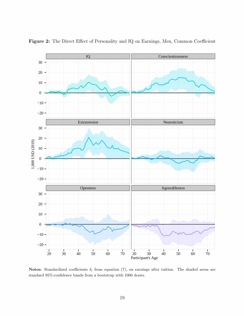
Figure 2: The Direct Effect of Personality and IQ on Earnings, Men, Common Coefficient

IQ Conscientiousness

Extraversion Neuroticism

Openness Agreeableness

−20

−10

0

10

20

30

−20

−10

0

10

20

30

−20

−10

0

10

20

30

20 30 40 50 60 70 20 30 40 50 60 70Participant's Age

1,00

0 U

SD

(20

10)

Notes: Standardized coefficients δt from equation (7), on earnings after tuition. The shaded areas are

standard 95%-confidence bands from a bootstrap with 1000 draws.

19

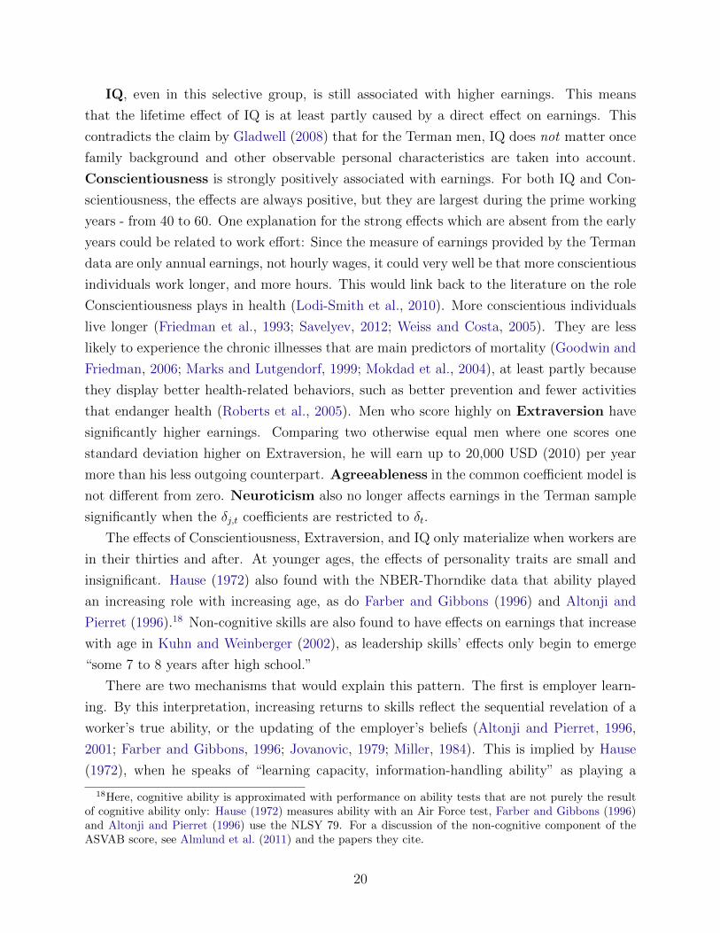
IQ, even in this selective group, is still associated with higher earnings. This means

that the lifetime effect of IQ is at least partly caused by a direct effect on earnings. This

contradicts the claim by Gladwell (2008) that for the Terman men, IQ does not matter once

family background and other observable personal characteristics are taken into account.

Conscientiousness is strongly positively associated with earnings. For both IQ and Con-

scientiousness, the effects are always positive, but they are largest during the prime working

years - from 40 to 60. One explanation for the strong effects which are absent from the early

years could be related to work effort: Since the measure of earnings provided by the Terman

data are only annual earnings, not hourly wages, it could very well be that more conscientious

individuals work longer, and more hours. This would link back to the literature on the role

Conscientiousness plays in health (Lodi-Smith et al., 2010). More conscientious individuals

live longer (Friedman et al., 1993; Savelyev, 2012; Weiss and Costa, 2005). They are less

likely to experience the chronic illnesses that are main predictors of mortality (Goodwin and

Friedman, 2006; Marks and Lutgendorf, 1999; Mokdad et al., 2004), at least partly because

they display better health-related behaviors, such as better prevention and fewer activities

that endanger health (Roberts et al., 2005). Men who score highly on Extraversion have

significantly higher earnings. Comparing two otherwise equal men where one scores one

standard deviation higher on Extraversion, he will earn up to 20,000 USD (2010) per year

more than his less outgoing counterpart. Agreeableness in the common coefficient model is

not different from zero. Neuroticism also no longer affects earnings in the Terman sample

significantly when the δj,t coefficients are restricted to δt.

The effects of Conscientiousness, Extraversion, and IQ only materialize when workers are

in their thirties and after. At younger ages, the effects of personality traits are small and

insignificant. Hause (1972) also found with the NBER-Thorndike data that ability played

an increasing role with increasing age, as do Farber and Gibbons (1996) and Altonji and

Pierret (1996).18 Non-cognitive skills are also found to have effects on earnings that increase

with age in Kuhn and Weinberger (2002), as leadership skills’ effects only begin to emerge

“some 7 to 8 years after high school.”

There are two mechanisms that would explain this pattern. The first is employer learn-

ing. By this interpretation, increasing returns to skills reflect the sequential revelation of a

worker’s true ability, or the updating of the employer’s beliefs (Altonji and Pierret, 1996,

2001; Farber and Gibbons, 1996; Jovanovic, 1979; Miller, 1984). This is implied by Hause

(1972), when he speaks of “learning capacity, information-handling ability” as playing a

18Here, cognitive ability is approximated with performance on ability tests that are not purely the resultof cognitive ability only: Hause (1972) measures ability with an Air Force test, Farber and Gibbons (1996)and Altonji and Pierret (1996) use the NLSY 79. For a discussion of the non-cognitive component of theASVAB score, see Almlund et al. (2011) and the papers they cite.

20

“larger role in earnings differentials over time as employers see improvement in the perfor-

mance of people as they gain experience.” These are opposed to skills that can be identified

from school transcripts (compare to Spence, 1973). Initially, as employers do not yet ob-

serve a person’s character traits or social skills, they cannot price these skills into wages.

But while this explanation of rising returns to skills over time is a sound economic argument,

the empirical evidence for this hypothesis in the context of personality traits is rather weak.

The coefficients on interactions of skills with actual tenure are insignificant in Heineck and

Anger (2010), Heineck (2011), and Nyhus and Pons (2005).

The second hypothesis that could explain the evolution of effects of social skills on wages

with increasing experience is related to occupational sorting and hierarchies. Possibly, social

skills start to matter meaningfully only once the worker has climbed the lowest rungs of the

ladder and is in a leadership position himself. While being extraverted and conscientious is

appreciated by his superiors at all levels, even while he is just an unimportant team member,

these traits have a reasonably larger impact on other team members and, therefore, overall

productivity, once he supervises others himself. This explanation is more directly related to

the nature of these non-cognitive skills.

Having access to data that combines measures of personality traits and IQ with long

follow-up is essential to pick up on this shape of effects by age. One can only describe the

effects of these traits in a satisfying manner with earnings measures that extend well into the

prime working years. Researchers who only have access to earnings observations for the early

working life would likely find that these personality traits have no significant association, or

very small ones, with earnings.19

For women, the estimates of direct effects of personality traits and IQ on earnings are

generally more noisy than for men. The effect estimates are never statistically significant in

19A caveat about causality is in order. In contrast to the estimated effect of education on earnings, whichcan be interpreted as causal under the assumptions of this paper, the estimated effect of personality should beinterpreted with caution. Researchers have debated whether reverse causality is a serious threat to validity inthe analysis of the effect of personality on earnings. They are concerned with the possibility that personalitytraits in mid-life are affected by past earnings and labor market experiences. Then, an association of acertain trait with earnings is not necessarily causal. Most researchers use early measures of personality, sothat these pre-date the outcome measures. This timing of measurements makes the interpretation of traitscausing outcomes more credible. Yet, early traits are not hypothesized to cause outcomes, but concurrenttraits. Thus, this method comes at the cost of not using the measure of personality that drives observedearnings (see Almlund et al., 2011).This paper follows the approach of using early measures of IQ, Openness and Extraversion. However, theother personality traits are measured in 1940 — when the Terman participants are 25-35 years old. Whileclaims of causality have to be guarded, the results can be interpreted as showing earnings gains due topersonality and IQ. A robustness analysis was performed to test whether the 1940 measures of personalitytraits are a function of early labor market success. The personality factors were extracted conditionally onwages prior to 1940, wages at age 25, education, and age. The estimated effects of these conditional factorson wages are very similar to those of unconditional factors (see Web Appendix C, Section C.7).

21

the age-by-age version. The full set of figures for own and husband’s earnings separately are

therefore relegated to the Web Appendix, Section C.1.

5 Educational Attainment as a Function of Psycholog-

ical Traits

Academic achievement and educational attainment have long been linked to IQ, motivation,

and personality traits. An emerging economic literature has also shown psychological traits

to be linked to educational attainment (Heckman et al., 2006). A summary is provided

by Almlund et al. (2011), who report on findings from representative datasets in the U.S.,

The Netherlands, and Germany. Conscientiousness is consistently found to have a strong

association with years of education. Its effect is the strongest among the psychological

traits, and its magnitude exceeds that of IQ. More conscientious individuals stay in school

longer. Extraversion, Agreeableness, and Neuroticism have weaker associations with edu-

cation. Openness exhibits a positive association, but is known to be moderately correlated

with IQ. Hence this finding could reflect the role of IQ rather than an own independent

relation to schooling if IQ is not controlled for.

Based on a generalized ordered logit model of education choice, presented in Table 3,

psychological traits in Terman play roles similar to those in the literature, but the effects

differ substantially by level of education, and by gender.

Conscientiousness is generally associated with higher schooling attainment, even con-

trolling for all background factors and other psychological traits. It is often found to be the

strongest predictor of academic achievement, as in the survey by Noftle and Robins (2007).

Conscientiousness likely enhances education through lowering the psychic costs of education,

lowering the discount rate, and helping to imagine the future better. The “hard working”

element of Conscientiousness implies that a conscientious person perceives the effort needed

to achieve a higher educational attainment as less costly. The “future planning” element of

Conscientiousness can be associated with lower discount rates for deferred gains. A greater

propensity to plan for the future could decrease the effort needed to imagine future out-

comes and to correctly evaluate the costs and gains involved in the long-term investments of

obtaining higher education.

Openness is also significantly associated with higher education levels in the Terman

sample, even conditioning on IQ. The effects of other psychological traits differ by gender.

IQ significantly increases the chances of obtaining at least some college for Terman men.

The associations between education and Extraversion, Agreeableness, and Neuroti-

22

Table 3: The Role of Psychological Traits on Education

Marginal Effects of Generalized Ordered Logit

Males Females

HSIQ −0.034

∗∗∗(−3.13) −0.008 (−1.16)

Openness 0.004 (0.46) −0.000 (−0.02)Conscientiousness −0.018

∗∗(−2.48) −0.003 (−0.26)

Extraversion −0.021∗

(−1.93) 0.024∗∗

(2.30)Agreeableness −0.005 (−0.52) 0.040

∗∗(2.49)

Neuroticism 0.005 (0.50) 0.050∗∗∗

(2.81)

Some CollegeIQ −0.003 (−0.16) −0.034 (−1.38)Openness −0.051

∗∗(−2.55) −0.011 (−0.35)

Conscientiousness −0.062∗∗∗

(−3.65) −0.059∗

(−1.78)Extraversion 0.017 (0.77) 0.022 (0.74)Agreeableness 0.031 (1.41) −0.016 (−0.41)Neuroticism −0.060

∗∗(−2.44) −0.027 (−0.64)

BAIQ 0.008 (0.36) 0.050 (1.41)Openness 0.014 (0.48) −0.048 (−1.17)Conscientiousness −0.038 (−1.42) −0.025 (−0.59)Extraversion −0.007 (−0.22) −0.046 (−1.29)Agreeableness −0.042 (−1.31) −0.009 (−0.19)Neuroticism 0.024 (0.64) −0.011 (−0.22)

MAIQ 0.016 (0.86) 0.005 (0.06)Openness −0.009 (−0.38) 0.033 (0.19)Conscientiousness 0.028 (1.05) 0.080 (1.42)Extraversion 0.003 (0.11) 0.020 (0.15)Agreeableness −0.016 (−0.54) −0.003 (−0.03)Neuroticism 0.046 (1.31) 0.005 (0.04)

PhDIQ 0.012 (0.59) −0.013 (−0.15)Openness 0.042 (1.62) 0.026 (0.15)Conscientiousness 0.091

∗∗∗(3.55) 0.007 (0.15)

Extraversion 0.008 (0.28) −0.020 (−0.15)Agreeableness 0.032 (1.05) −0.012 (−0.15)Neuroticism −0.016 (−0.45) −0.017 (−0.15)

Notes: Marginal effects from a generalized ordered logit model, evaluated at means of all covariates

(standard errors in parentheses). Estimated using Williams (2006) with standard controls in Table 1, of

which a number are constrained to equal coefficients without rejecting H0 of proportional odds. Asterisks

denote statistical significance based on a two-sided asymptotic test;* p < .1, ** p < .05, *** p < .01.

23

cism for Terman females are similar to findings in previous studies, where representative

samples of men and women were used. All effects are negative. One expects a negative

effect from extraversion as socializing takes time away from studies. This has been found by

O’Connell and Sheikh (2011), for example. The associations for Terman males diverge from

previous studies, as they are now treated separately instead of pooling them with women.

For Terman men, extraversion has no significant effect on educational attainment, and neu-

roticism even seems to have a positive impact on education. Both of these findings contradict

established knowledge from representative pooled samples.

6 The Rate of Return to Schooling

Having established that psychological traits determine educational choice, we can ask how

education translates into lifetime earnings. One common way of summarizing this informa-

tion is through the internal rate of return (IRR).20 Standard procedures developed by Becker

and Chiswick (1966) and Mincer (1974) make strong assumptions to use cross sectional data

to estimate life-cycle rates of return.21 Because the Terman data provides complete life-cycle

earnings data, these assumptions are not necessary here. Also, instead of relying on years

of schooling as the regressor, I contrast different levels of education in pairwise comparisons.

This yields a richer picture of the different trade-offs that individuals face when choosing

one education level over another. The Mincer specification performs poorly in comparison.

Furthermore, a drastic departure from the traditional rate-of-return analysis results from

the interactions established in Section 4. The rate of return to education is significantly

higher for men who are highly extroverted, conscientious, and emotionally stable.

6.1 The Mincer Coefficient

Most rates of return in the literature are not actually estimates of the internal rate of return.

It is common practice to estimate a Mincer equation and interpret the coefficient on years

of schooling as the rate of return. Even though the Terman data are longitudinal, one can

estimate the Mincer equation as if the data were cross-sectional. Regressing log wages on

years of schooling, experience and its square, the Terman Mincer rate of return for males is

7.5%. For women, it is 6.0%, and for their family earnings it is only 3.6%.22

20This is the discount rate that would make an individual indifferent between two options: obtaining more

education or remaining at a baseline level (j vs. k). It is the ρ that solves the polynomial∑75t=18

(κj,t−κk,t)

(1+ρ)t= 0.

From Eq. (1), we have the causal effects of education κj,t at all ages t = 18, ..., 75.21Heckman et al. (2006) review the literature which is based on this approach.22For this comparison, all observations in the treatment-estimation sample are used, ages 18-65, as if they

were from a cross-section. Years of schooling are imputed from degrees and experience is approximated

24

The standard Mincer regression does not include other covariates, but if personality traits

are included as regressors, the Mincer coefficient for men drops to 6.5%, and it drops further

to 6.3% when IQ is controlled for. This decrease is commonly associated with “ability bias”

(Griliches, 1977) - even though most researchers have only cognitive ability or IQ in mind

and not other aspects of ability. In comparison to Blackburn and Neumark (1995), the

decrease in the Terman data from including IQ is much smaller than their 40%. In this

sample with a restricted IQ range, omitting non-cognitive abilities or personality traits is of

greater importance.

In comparison to the numbers one typically expects for Mincer coefficients, the 7.5% for

men is at the OECD average during the 1990s (Psacharopoulos and Patrinos, 2004), but

lower than typical US figures (Card, 1999). Of course, these well-known Mincer estimates

are for more recent cohorts and a comparison with estimates from the 1950 census23 is more

appropriate. The Mincer coefficient for synthetic cohorts from the 1950 census is 9%, which

is still higher than the Terman estimate. In fact, if the Terman earnings were top-coded as

in the census, the Mincer rate of return would only be 3.9%. These comparisons might lead

us to conclude that returns to education at the very high end of IQ are low, that “geniuses”

do not need formal training. This conclusion would be faulty, however, as the Mincer return

does not correspond to the true pairwise rates of return, and masks a large variation in

returns that can be observed for the different education levels.

6.2 The IRR for Men

The average treatment effect of education level j vs. k at each age t corresponds to κj,t−κk,tfrom Eq. (1). At the mean, factor scores are zero, therefore in these average effects, the

impact of psychological traits drops out.24

The pairwise estimates of average treatment effects are plotted in the top graphs of

Table 4. Schooling always has a negative effect on annual earnings in the early years of

a working life since individuals who are obtaining more education are still in school while

their peers with less education are already out of school and working. The following positive

effect of education is substantial during the prime working years, a standard result in the

literature (Becker, 1964).

by subtracting six and the number of years of schooling from the participant’s current age. Log wages areregressed on years of schooling, experience, and its square. In a second estimation, the regressors are enrichedby the set of psychological traits and background variables as in our standard estimation.

23The IPUMS sample, described by Ruggles et al. (2010), was used.24This means that the second term, θ(δj,t−δk,t), evaluates to zero at the mean, since the θ have mean zero.

In the limit, the average treatment effect of education as estimated from Eq. (1) is equal to the estimatesfrom Eq. (7), as the personality traits and IQ are normalized to have mean zero.

25

Table 4: Select Pairwise Average Treatment Effects on Earnings, Males

IRR = 11.3C.I. = [−18.5, 27.1]Sum = 340.912

IRR = 12.5C.I. = [4.8, 18.7]Sum = 1106.151

IRR = 8.5C.I. = [3.8, 13.4]Sum = 1027.799

IRR = 9.3C.I. = [5.9, 12.7]Sum = 1701.446

Some College vs High School Bachelor's vs High School

Master's vs High School Doctorate vs High School−50

0

50

100

−50

0

50

100

20 30 40 50 60 70 20 30 40 50 60 70Age

Tre

atm

ent E

ffect

, 1,0

00 U

SD

Some Coll. Bachelor Master Doctorate Some Coll. Bachelor Master Doctorate

High School 11.3 12.5 8.5 9.3 116.5 379.2 302.2 497.6[-18.5, 27.1] [4.8, 18.7] [3.8, 13.4] [5.9, 12.7] [-165, 385] [113, 645] [20, 584] [233, 787]

Some College 13.4 7.5 8.9 264.8 187.8 383.2[-0.3, 21.4] [2.4, 13.7] [5.4, 12.6] [39, 480] [-51, 431] [155, 644]

Bachelor -2.3 5.9 -75.0 120.5[-13.8, 63.8] [1.5, 11.6] [-286, 139] [-90, 335]

Master 13.0 197.4[-4.2, 23.7] [-4, 413]

Internal Rate of Return Net Present Value, discounted at 3%

Notes: The graphs show age-by-age treatment effects from Eq. (1), with 95% confidence bands, and list

the net (undiscounted) lifetime effect of education in “Sum,” whereas the table lists the net present value

discounted at 3%. The effects are evaluated for males with average personality traits, and confidence bands

are from 1000 bootstrap draws. Earnings are annual earnings after tuition in 2010 U.S. Dollars, with the top

3% of values truncated. Covariates are IQ, factor scores for personality traits, parental background, family

environment, childhood health, and controls for WWII and cohort. The full set of treatment effect curves

are available in Web Appendix Section C.1.

26

Each graph lists the IRR corresponding to the estimated average effects, and the effect

of schooling on the (undiscounted) sum of lifetime earnings. The complete set of IRRs and

discounted net present values are then given in the bottom of Table 4. 25

The pairwise treatment effects are clearly different from each other and cannot be sum-

marized in a single “rate of return” as one would obtain from the Mincer coefficient. In

comparison to having a high school diploma, obtaining a bachelor’s degree increases the Ter-

man males’ earnings by a total of $1,106,151 over a lifetime, or $379,200 if the difference in

earnings is discounted at 3%. The corresponding IRR is 12.5%. This estimate implies that

even for the highly talented Terman men with IQs above 140, going to school substantially

contributed to increasing their lifetime earnings, and the rate of return to this investment

exceeds that of the return on equity.26

How does this compare to an estimate from the census? If we estimate the differences

between schooling levels nonparametrically as in Heckman et al. (2006), and treat the Terman

data as census data (including top-coding), we obtain Fig. 3. With this methodology, the

average wage gain from a bachelor’s degree in Terman is lower than from the matching

methodology (where earnings are not top-coded, either). The Terman IRR is now smaller

than the census return, despite the higher earnings of Terman men. The reason is that at

both education levels, Terman earnings are higher - therefore, education makes a smaller

relative difference. Since Terman men with a high school diploma earn substantially more

than the average man from the census, the opportunity cost of schooling is much higher.

If we had not top-coded the Terman earnings, the IRR from this methodology would have

been closer to the census, at 11.4% Of course, in this exercise none of the rich background

variables or human capital measures from the Terman survey are used.

Returning to the causal estimates from the matching procedure, Table 4 shows that the

average return to a doctoral degree in comparison to a bachelor’s increases lifetime earnings,

but has an IRR of only 5.9%. And for the person with average levels of all psychological

traits, obtaining a master’s degree over a bachelor’s has a negative IRR at -2.3%..

Looking at IRRs only could lead us to the conclusion that post-graduate degrees are

worse investments than a simple college degree, but the IRRs hide the net lifetime values

which accurately reflect the large absolute gains that outweigh the long up front investments.

25In principle, an IRR should be compared to the market interest rate to determine the optimality ofschooling. IRRs are not suited to compare three alternative investments to each other (Ross et al., 2001).For example, the IRR of “some college” over high school is very similar to that of a bachelor’s over highschool— but this is a result only of the small up front costs, combined with small absolute gains later on.The net present value is better suited to compare several alternatives, and it shows that the bachelor’s is aninvestment that is more attractive (net gains of $379,200 rather than $116,400).

26The S&P 500 annualized return from 1928 to 1985 (when the Terman men were on average 18–75 yearsold), is about 6%.

27

Figure 3: IRR and Mean Earnings by Education in Terman and Census, Males

IRR Terman = 8.6NPV Terman = 173,147

-IRR Census = 10.7

NPV Census = 146,865

010

2030

4050

6070

LLR

Est

imat

e of

Ear

ning

s, in

100

0 U

SD

(20

10)

20 25 30 35 40 45 50 55 60 65 70

Age

Terman, High School Terman, College level

Census, High School Census, College level

Notes: Local linear regression estimates of earnings in Terman and 1950 census, as in Heckman et al. (2006),

comparing census men with 12 and 16 years of schooling to Terman men with a high school diploma only

(no college) and a bachelor’s degree. Terman earnings are treated as census data, and are topcoded at the

1950 values. All earnings are set to zero during college. Net present values are discounted at 3%.

28

At IRRs of 8.5% and 9.3%, the doctoral degree leads to even higher lifetime earnings gains

than the master’s degree (about $1.7 million vs $1.0 million ).

Furthermore, these are average effects in the sense that they are the effect of education

on earnings evaluated at average levels of all psychological traits. The significant interaction

between education and these traits means that a man with certain traits stands to gain

substantially from obtaining a postgraduate degree, as it will enable him to reap the higher

reward to his traits. For example, a man at the 80th percentile of Extraversion would expect

a lifetime return from obtaining a master’s degree (versus high school) of $ 1.4 million, but

someone at the 20th percentile only $0.7 million.

Even in a high ability group, education adds skills that are valued on the marketplace.

The returns to schooling are real, and ability bias cannot be responsible for the type of

returns we find.

6.3 The IRR for Women, Family Earnings Decomposed

The women in the Terman sample belonged to a generation in which the role of the woman

was still mainly that of a homemaker, mother, and wife. Society defined very strictly what

type of occupations were deemed “suitable” for a woman, and a woman’s freedom to choose

her career or define her own lifestyle was not what it is today. Thus, a high share of house-

wives should be expected among the Terman women. About half of the Terman women did

not engage in paid work, despite their extraordinary abilities and talents. Many housewives

did not earn a market wage, but these women could still benefit from education by finding

a better match, a husband with higher educational achievement and earnings, and thus in-

crease their potential family earnings. A Terman woman with postgraduate education was

more likely to be in gainful employment and less likely to be married than her peers with at

most a Bachelor’s degree, as Fig. 4 shows. Whether this relationship between education and

labor supply or marital status is causal is far from clear. For example, a highly educated

woman might have chosen to focus her energy on a career early on, and with own earnings

would have been less dependent on finding a husband. Also, her high education and career

aspirations may have made her less attractive as a marriage partner. It is also possible that

causality moves in the other direction. For example, she might not have found a husband

initially, and thus decided to obtain more schooling in order to support herself.

Women with post-graduate education greatly improved their own earnings (see Fig. 5).

The treatment effect of a master’s degree is positive but remains small and is not statistically

significant. For women with a doctorate degree, the returns to education are substantial,

and even higher in terms of IRRs than men’s.

29

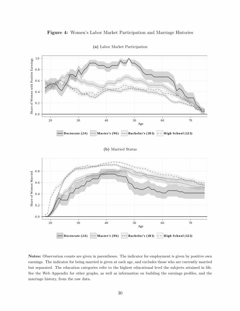
Figure 4: Women’s Labor Market Participation and Marriage Histories

(a) Labor Market Participation

0.0

0.2

0.4

0.6

0.8

1.0

20 30 40 50 60 70Age

Shar

e of

Wom

en w

ith

Pos

itiv

e E

arn

ings

Doctorate (24) Master's (96) Bachelor's (181) High School (121)

(b) Married Status

0.0

0.2

0.4

0.6

0.8

20 30 40 50 60 70Age

Shar

e of

Wom

en M

arri

ed

Doctorate (24) Master's (96) Bachelor's (181) High School (121)

Notes: Observation counts are given in parentheses. The indicator for employment is given by positive own

earnings. The indicator for being married is given at each age, and excludes those who are currently married

but separated. The education categories refer to the highest educational level the subjects attained in life.

See the Web Appendix for other graphs, as well as information on building the earnings profiles, and the

marriage history, from the raw data.

30

Figure 5: Pairwise Treatment Effects on Own Earnings, Females

IRR = NAC.I. = [NA, NA]Sum = −58.634

IRR = 18.4C.I. = [9, 27]Sum = 1037.775

IRR = 16.5C.I. = [7.1, 30.1]Sum = 195.975

IRR = 22.1C.I. = [5.4, 77.5]Sum = 1096.44

IRR = 27.7C.I. = [−0.1, 81.2]Sum = 254.64

IRR = 20.0C.I. = [5.4, 73.6]Sum = 842.223

Bachelor's vs High School Doctorate vs High School

Master's vs High School Doctorate vs Bachelor's

Master's vs Bachelor's Doctorate vs Master's

−25

0

25

50

75

−25

0

25

50

75

−25

0

25

50

75

20 30 40 50 60 70 20 30 40 50 60 70Age

Tre

atm

ent E

ffect

, 1,0

00 U

SD

Notes: Average treatment effects of education on own earnings, from the estimation of Eq. (1). Correspond-

ing to these lifetime effects are the internal rate of return (IRR) with bootstrapped 95% confidence bands

(1000 draws), and the net effect on total lifetime earnings (Sum). The effects are evaluated for females with

average personality traits, earnings are annual earnings after tuition in 2010 U.S. Dollars, with the top 3%

of values truncated. See the appendix for effects on discounted earnings (NPV).

31

Figure 6 decomposes the effect of education on women’s family earnings into its effect

on their own earnings and on their husband’s earnings (which is the effect through marriage).

The combined effect of education on family earnings is shown in the solid black line, and

the corresponding IRRs are shown in the box. The treatment effect on family earnings is

dominated by the very large effect on their own earnings for women with a doctoral degree

— it completely washes out the slightly negative effect that education has on husband’s

earnings. But these women were very special cases. They worked in high-ranking jobs, had

high earnings, and did not rely on their husbands to provide their earnings.

The returns to education in terms of family earnings are also positive for women with

a bachelor’s degree, because they benefit from the marriage market. Again, the gains

from education through marriage through husband’s earnings can be decomposed into

the effect of education on the probability of being married, and on conditional husband’s

earnings.

The gains from education are positive for women with a bachelor’s degree over high

school. Yet for education levels beyond the bachelor’s, higher education is associated with

slightly lower earnings through marriage. The more highly educated women are less likely to

be married, and thus lose the opportunity to bolster their own earnings with their husband’s.

Thus, the rate of return is negative because the return through own earnings is not enough

to offset the losses in the marriage market.27

Figure 7 explores these different effects: It shows two counterfactual treatment effects

of education on the women’s gains through marriage. The first counterfactual describes

the case when the propensity to be married did not differ by education. Say, it is one for

all education groups. The solid line represents this case where education only affects the

quality of matches. For women with a bachelor’s or doctorate degree, education improves

match quality. Women with a master’s were not able to find higher-earning husbands than

less-educated women, leading to a negative return through match quality.

The second counterfactual describes the environment where the propensity to be married

is influenced by education, but the match quality is not. In that case, husbands’ earnings

were the same regardless of the woman’s education.

The dashed line corresponding to this second counterfactual shows that marriage prospects

clearly declined increasingly with education past a bachelor’s degree. The lower marriage

propensity outweighs the effect of education on match quality, leading to negative returns

to education through husbands.

27The rate of return of a master’s degree over the high school diploma cannot be computed because thereare multiple crossings with the zero line, and there might simply not exist a rate of return that would setthe net present value of this investment to zero.

32

Figure 6: Pairwise Treatment Effects on Earnings and Decomposition, Females

Family Earnings: IRR = 17.3CI = [6.6, 34.1]Sum = 144.431

Family Earnings: IRR = 17.3CI = [6.6, 34.1]Sum = 144.431

Family Earnings: IRR = 17.3CI = [6.6, 34.1]Sum = 144.431

Family Earnings: IRR = 12.5CI = [1.6, 44.1]Sum = 566.563

Family Earnings: IRR = 12.5CI = [1.6, 44.1]Sum = 566.563

Family Earnings: IRR = 12.5CI = [1.6, 44.1]Sum = 566.563

Family Earnings: IRR = −0.5CI = [−18.4, 37.7]Sum = −7.293

Family Earnings: IRR = −0.5CI = [−18.4, 37.7]Sum = −7.293

Family Earnings: IRR = −0.5CI = [−18.4, 37.7]Sum = −7.293

Family Earnings: IRR = 9.9CI = [−38.3, 49.5]Sum = 422.435

Family Earnings: IRR = 9.9CI = [−38.3, 49.5]Sum = 422.435

Family Earnings: IRR = 9.9CI = [−38.3, 49.5]Sum = 422.435

Family Earnings: IRR = −3.4CI = [−86.7, 32]Sum = −151.421

Family Earnings: IRR = −3.4CI = [−86.7, 32]Sum = −151.421

Family Earnings: IRR = −3.4CI = [−86.7, 32]Sum = −151.421

Family Earnings: IRR = 20.0CI = [−22.1, 63]Sum = 574.678

Family Earnings: IRR = 20.0CI = [−22.1, 63]Sum = 574.678

Family Earnings: IRR = 20.0CI = [−22.1, 63]Sum = 574.678

Bachelor's vs High School Doctorate vs High School

Master's vs High School Doctorate vs Bachelor's

Master's vs Bachelor's Doctorate vs Master's

−40

−20

0

20

40

60

80

−40

−20

0

20

40

60

80

−40

−20

0

20

40

60

80

20 30 40 50 60 70 20 30 40 50 60 70Participant's Age

Tre

atm

ent E

ffect

, in

1,00

0 U

SD

(20

10)

Treatment Effect Family Earnings w 95% Conf.Int. Husband's Earn. Own Earn.

Notes: Average treatment effects from estimation Eq. (1), on three measures of annual earnings in 2010 U.S.

Dollars: Terman female’s earnings, their husband’s earnings, and the combined family earnings (solid black

line, light grey area is the 95% confidence band from 1000 bootstrap draws). Corresponding to these lifetime

effects are the internal rate of return (IRR) with bootstrapped 95% confidence bands, and net present value

(NPV) at a 3% discount rate.

33

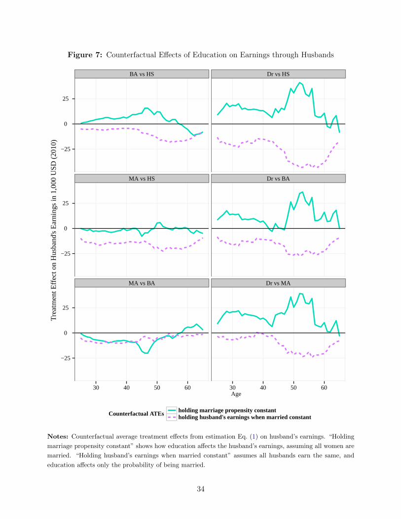
Figure 7: Counterfactual Effects of Education on Earnings through Husbands

BA vs HS Dr vs HS

MA vs HS Dr vs BA

MA vs BA Dr vs MA

−25

0

25

−25

0

25

−25

0

25

30 40 50 60 30 40 50 60Age

Tre

atm

ent E

ffect

on

Hus

band

's E

arni

ngs

in 1

,000

US

D (

2010

)

Counterfactual ATEs holding marriage propensity constantholding husband's earnings when married constant

Notes: Counterfactual average treatment effects from estimation Eq. (1) on husband’s earnings. “Holding

marriage propensity constant” shows how education affects the husband’s earnings, assuming all women are

married. “Holding husband’s earnings when married constant” assumes all husbands earn the same, and

education affects only the probability of being married.

34

Most interestingly, the exceptional women who obtained a doctorate degree did not suffer

significantly in the marriage market, as one might have anticipated. Even though they were

significantly less likely to be married, conditional on being married, their husbands had

higher-than-average earnings, so the overall impact of their high education on the returns to

marriage are not statistically different from zero.

In the lifetimes of the Terman cohort, women’s opportunities to increase their earnings

through education were more limited for women than they were for men. Women’s own

earnings mostly fell short of the earnings of men with the same level of education and ability;

not only due to the choice of occupation, but also within occupation. At the same time,

marriage prospects were not always boosted by higher education, and only increased earnings

sufficiently for women with a college education to offset their smaller market returns. For

them, the rates of return to education were similar to those of Terman men.

7 Conclusion

This paper estimates the effects of personality traits and IQ on lifetime earnings of the high-

achieving men and women of the Terman study. Personality traits and IQ affect the levels

of earnings, especially in the prime working years. They also affect educational sorting and

thus command an indirect effect on lifetime earnings. Furthermore, there is a significant

interaction between education and traits in producing earnings. Therefore, the treatment

effect of schooling is a function of personality traits. By the unique access to the full lifetime

earnings histories, these heterogeneous effects can be disentangled, whereas in an age-by-age

estimation, they fail to be statistically significant.

Psychological traits are rewarded directly in the marketplace for men, but not for women

of this cohort. Men gain from traits such as Conscientiousness, Extraversion, and IQ. Women

with up to a Bachelor’s degree are able to gain from Extraversion by matching to higher-

earning partners.

The presented estimates of the internal rate of return to education do not rely on the

strong assumptions that are standard in the literature to estimate the “rates of return.”

Instead, the returns are based on causal effects, obtained by matching on an unusually

extensive list of covariates, including IQ and personality. The analysis of the returns to

education for persons at the high end of the IQ distribution is unique.

The returns for the Terman men are sizeable. For women at education levels below the

doctoral level, the rates of return are low. But there are gains through sorting in the marriage

market for women with a college education. Women with a doctorate degree have very high

earnings on their own, and their rates of return are even higher than those of men.

35

The findings presented here contribute to the literature on childhood interventions that

focus on social skills. Social skills or personality traits have profound influences on life out-

comes and they are more malleable past early childhood than, for example, IQ. Therefore,

they point to a promising avenue of reducing inequality and providing development oppor-

tunities, which actually circumvent the traditional efficiency-equity tradeoff due to their

positive rates of return. The literature has not yet analyzed whether personality traits play

a similarly important role for children at the other end of the spectrum (i.e., high-ability

children). This paper shows that indeed, men earn substantially more if they possess strong

social skills. The increase in discounted lifetime earnings corresponds to about half of the

effect of obtaining a bachelor’s degree over high school only. Highly-able individuals are

therefore also likely to benefit from interventions targeted at improving their social skills.

36

References

Almlund, M., A. L. Duckworth, J. J. Heckman, and T. Kautz (2011). Personality Psychologyand Economics. In E. A. Hanushek, S. Machin, and L. Woessmann (Eds.), Handbook ofthe Economics of Education, Vol. 4, Volume 4, Chapter 1, pp. 1–181. Elsevier B.V.

Altonji, J. G. and C. R. Pierret (1996). Employer Learning and the Signaling Value ofEducation. NBER Working Paper Series (5438).

Altonji, J. G. and C. R. Pierret (2001). Employer Learning and Statistical Discrimination.The Quarterly Journal of Economics 116 (1), 313–350.

Barrick, M. R. and M. K. Mount (1991). The Big Five Personality Dimensions and JobPerformance: A Meta-Analysis. Personnel Psychology 44 (1), 1–26.

Bartlett, M. (1937). The Statistical Conception of Mental Factors. British Journal of Psy-chology 1 (28), 97–104.

Becker, G. S. (1964). Human Capital: A Theoretical and Empirical Analysis, With SpecialReference to Education. New York: National Bureau of Economic Research.

Becker, G. S. and B. R. Chiswick (1966). Education and the Distribution of Earnings. TheAmerican Economic Review 56 (1/2), 358–369.

Becker, G. S., E. M. Landes, and R. T. Michael (1977). An Economic Analysis of MaritalInstability. Journal of Political Economy 85 (6), 1141–1187.

Blackburn, M. L. and D. Neumark (1995). Are OLS Estimates of the Return to SchoolingBiased Downward? Another Look. The Review of Economics and Statistics 77 (2), 217–230.

Bolck, A., M. Croon, and J. Hagenaars (2004). Estimating Latent Structure Models withCategorical Variables: One-Step Versus Three-Step Estimators. Political Analysis 12 (1),3–27.

Boudreau, J. W., W. R. Boswell, and T. A. Judge (2001). Effects of Personality on ExecutiveCareer Success in the United States and Europe. Journal of Vocational Behavior 58 (1),53–81.

Bowles, S., H. Gintis, and M. Osborne (2001). Incentive-Enhancing Preferences: Personality,Behavior, and Earnings. The American Economic Review 91 (2), 155–158.

Card, D. (1999). The Causal Effect of Education on Earnings. In O. Ashenfelter andD. Card (Eds.), Handbook of Labor Economics, Vol. 3, Volume 3, Chapter 30, pp. 1801–1863. Elsevier Science B.V.

Costa, P. T. J. and R. R. McCrae (1994). Set like Plaster? Evidence for the Stability ofAdult Personality. In T. F. Heatherton and J. L. Weinberger (Eds.), Can personalitychange?, pp. 21–40. Washington, D.C., U.S.A.: American Psychological Association.

37

Croon, M. (2002). Using Predicted Latent Scores in General Latent Structure Models. InG. A. Marcoulides and I. Moustaki (Eds.), Latent Variable and Latent Structure Models,Chapter 10, pp. 195–223. Lawrence Erlbaum Associates, Inc.

Dauber, S. L. and C. P. Benbow (1990). Aspects of Personality and Peer Relations ofExtremely Talented Adolescents. Gifted Child Quarterly 34 (1), 10–14.

Eysenck, H. J. (1993). The Relationship between IQ and Personality. In G. L. Van Heck,P. Bonaiuto, I. J. Deary, and W. Nowack (Eds.), Personality psychology in Europe (Vol.4). Tilburg, The Netherlands: Tilburg University Press.

Farber, H. S. and R. Gibbons (1996). Learning and Wage Dynamics. Quarterly Journal ofEconomics (November), 1007–1047.

Friedman, H. S. (2000). Long-Term Relations of Personality and Health: Dynamisms, Mech-anisms, Tropisms. Journal of Personality 68 (6), 1089–107.

Friedman, H. S. (2008). The multiple linkages of personality and disease. Brain, Behavior,and Immunity 22 (5), 668–675.

Friedman, H. S. and L. R. Martin (2011). The Longevity Project: Surprising Discoveriesfor Health and Long Life from the Landmark Eight-Decade Study (1 ed.). Hudson StreetPress.

Friedman, H. S., J. S. Tucker, J. E. Schwartz, L. R. Martin, C. Tomlinson-Keasey, D. L.Wingard, and M. H. Criqui (1995a). Childhood Conscientiousness and Longevity: HealthBehaviors and Cause of Death. Journal of Personality and Social Psychology 68 (4), 696–703.

Friedman, H. S., J. S. Tucker, J. E. Schwartz, L. R. Martin, C. Tomlinson-Keasey, D. L.Wingard, and M. H. Criqui (1995b). Childhood Conscientiousness and Longevity: HealthBehaviors and Cause of Death. Journal of Personality and Social Psychology 68 (4), 696–703.

Friedman, H. S., J. S. Tucker, C. Tomlinson-Keasey, J. E. Schwartz, D. L. Wingard, andM. H. Criqui (1993). Does Childhood Personality Predict Longevity? Journal of Person-ality and Social Psychology 65 (1), 176–85.

Gladwell, M. (2008, November). Outliers: The Story of Success. New York, NY: Little,Brown and Company.

Goldberg, L. R. (1993). The Structure of Phenotypic Personality Traits. American Psychol-ogist 48 (1), 26–34.

Goldin, C. (1992). Understanding the Gender Gap: An Economic History of AmericanWomen. NBER Series on Long-Term Factors in Economic Development, Oxford UniversityPress.

38

Goldsmith, A. H., J. R. Veum, and W. J. Darity (1997). The Impact of Psychological andHuman Capital on Wages. Economic Inquiry XXXV (October), 815–829.

Goodwin, R. D. and H. S. Friedman (2006). Health Status and the Five-factor PersonalityTraits in a Nationally Representative Sample. Journal of Health Psychology 11 (5), 643–54.

Griliches, Z. (1977). Estimating the Returns to Schooling: Some Econometric Problems.Econometrica 45 (1), 1–22.

Grossman, J. B. and J. P. Tierney (1998). Does Mentoring Work? An Impact Study of theBig Brothers Big Sisters Program. Evaluation Review 22 (3), 403–426.

Hamermesh, D. S. (1984). Life-Cycle Effects on Consumption and Retirement. Journal ofLabor Economics 2 (3), 353–370.

Hause, J. C. (1972). Earnings Profile: Ability and Schooling. Journal of Political Econ-omy 80 (3, Part 2: Investment in Education: The Equity-Efficiency Quandary), S108–S138.

Heckman, J. J., L. J. Lochner, and P. E. Todd (2006). Earnings Functions, Rates of Returnand Treatment Effects: The Mincer Equation and Beyond. In E. A. Hanushek and F. Welsh(Eds.), Handbook of the Economics of Education, Vol. 1, Volume 1, Chapter 7, pp. 307–458. Elsevier B.V.

Heckman, J. J., S. H. Moon, R. Pinto, P. A. Savelyev, and A. Yavitz (2010). The rate ofreturn to the HighScope Perry Preschool Program. Journal of Public Economics 94 (1-2),114–128.

Heckman, J. J., R. Pinto, and P. A. Savelyev (2013). Understanding the MechanismsThrough Which an Influential Early Childhood Program Boosted Adult Outcomes. TheAmerican Economic Review 103 (6), 2052–2086.

Heckman, J. J. and R. Robb (1985). Using longitudinal data to estimate age, period andcohort effects in earnings equations. In W. M. Mason and S. E. Fienberg (Eds.), CohortAnalysis in Social Research: Beyond the Identification Problem. New York: Springer-Verlag.

Heckman, J. J., J. Stixrud, and S. Urzua (2006). The Effects of Cognitive and Noncog-nitive Abilities on Labor Market Outcomes and Social Behavior. Journal of Labor Eco-nomics 24 (3), 411–482.

Heineck, G. (2011). Does it Pay to be Nice? Personality and Earnings in the UnitedKingdom. Industrial and Labor Relations Review 64 (5), 1020–1038.

Heineck, G. and S. Anger (2010). The returns to cognitive abilities and personality traits inGermany. Labour Economics 17 (3), 535–546.

Hogan, R. and J. Hogan (2007). Hogan Personality Inventory Manual (3rd ed.). Tulsa, OK:Hogan Assessment Systems.

39

Holland, J. L., J. A. Johnston, N. F. Asama, and S. M. Polys (1993). Validating and Usingthe Career Beliefs Inventory. Journal of Career Development 19 (4), 233–244.

Hughes, J. (1986). The Vital Few. Oxford University Press, USA.

Jones, G. (2011). IQ and National Productivity. In S. N. D. Blume and L. E. (Eds.), TheNew Palgrave Dictionary of Economics (Online ed.)., pp. 1–6. Palgrave Macmillan.

Joreskog, K. and D. Sorbom (1979). Advances in Factor Analysis and Structural EquationModels. Cambridge, Massachusetts: Abt Books.

Jovanovic, B. (1979). Job Matching and the Theory of Turnover. The Journal of PoliticalEconomy 87 (5), 972–990.

Judge, T. A., J. E. Bono, R. Ilies, and M. W. Gerhardt (2002). Personality and Leadership:A Qualitative and Quantitative Review. Journal of Applied Psychology 87 (4), 765–780.

Judge, T. A., C. A. Higgins, C. J. Thoresen, and M. R. Barrick (1999). The Big FivePersonality Traits, General Mental Ability, and Career Success Across the Life Span.Personnel Psychology 52 (3), 621–652.

Judge, T. A., E. A. Locke, C. C. Durham, and A. N. Kluger (1998). Dispositional Effectson Job and Life Satisfaction: The Role of Core Evaluations. Journal of Applied Psychol-ogy 83 (1), 17–34.

Kuhn, P. and C. Weinberger (2002). Leadership Skills and Wages. IZA Discussion PaperSeries (482).

Leibowitz, A. (1974). Home Investments in Children. Journal of Political Economy 82 (2,Part 2: Marriage, Family Human Capital and Fertility (Mar.-Apr.)), S111–S131.

Leon, G. R., B. Gillum, R. Gillum, and M. Gouze (1979). Personality Stability and ChangeOver a 30-Year Period—Middle Age to Old Age. Journal of consulting and clinical psy-chology 47 (3), 517–24.

Lodi-Smith, J., J. Jackson, T. Bogg, K. Walton, D. Wood, P. Harms, and B. W. Roberts(2010). Mechanisms of health: Education and health-related behaviours partially mediatethe relationship between conscientiousness and self-reported physical health. PsychologicalHealth 25 (3), 305–319.

Mare, R. D. (1991). Five Decades of Educational Assortative Mating. American SociologicalReview 56 (1), 15–32.

Marks, G. R. and S. K. Lutgendorf (1999). Perceived Health Competence and PersonalityFactors Differentially Predict Health Behaviors in Older Adults. Journal of Aging andHealth 11 (2), 221–239.

Martin, L. R. and H. S. Friedman (2000). Comparing Personality Scales Across Time: AnIllustrative Study of Validity and Consistency in Life-Span Archival Data. Journal ofPersonality 68 (1), 85–110.

40

Martin, L. R., H. S. Friedman, K. M. Clark, and J. S. Tucker (2005). Longevity followingthe experience of parental divorce. Social Science and Medicine 61 (10), 2177–2189.

Martin, L. R., H. S. Friedman, and J. E. Schwartz (2007). Personality and mortality riskacross the life span: The importance of conscientiousness as a biopsychosocial attribute.Health Psychology 26 (4), 428–436.

Martin, L. R., H. S. Friedman, J. S. Tucker, C. Tomlinson-Keasey, M. H. Criqui, and J. E.Schwartz (2002). A Life Course Perspective on Childhood Cheerfulness and its Relationto Mortality Risk. Personality and Social Psychology Bulletin 28 (9), 1155–1165.

McCrae, R. R. and O. P. John (1992). An Introduction to the Five-Factor Model and ItsApplications. Journal of Personality 60 (2), 175–215.

Michael, R. T. (1976). Factors Affecting Divorce: A Study of the Terman Sample. NBERWorking Paper Series (147).

Miller, R. A. (1984). Job Matching and Occupational Choice. Journal of Political Econ-omy 92 (6), 1086.

Mincer, J. (1974). Schooling, Experience and Earnings. New York: Columbia UniversityPress for National Bureau of Economic Research.

Mokdad, A. H., J. S. Marks, D. F. Stroup, and J. L. Gerberding (2004). Actual Causesof Death in the United States, 2000. JAMA : The Journal of the American MedicalAssociation 291 (10), 1238–45.

Mount, M. K., M. R. Barrick, and L. Stewart (1998). Five-Factor Model of Personality andPerformance in Jobs Involving Interpersonal Interactions. Human Performance 11 (2-3),37–41.

Mulaik, S. A. (2010). Foundations of Factor Analysis (2nd ed.). Boca Raton, FL: Chapman& Hall/ CRC.

Muller, G. and E. Plug (2006). Estimating the Effect of Personality on Male and FemaleEarnings. Industrial and Labor Relations Review 60 (1), 3–22.

Murnane, R. J., J. B. Willett, M. J. Braatz, and Y. Duhaldeborde (2001). Do differentdimensions of male high school students’ skills predict labor market success a decadelater? Evidence from the NLSY. Economics of Education Review 20 (4), 311–320.

Murphy, K. M., A. Shleifer, and R. W. Vishny (1991). The Allocation of Talent: Implicationsfor Growth. The Quarterly Journal of Economics 106 (2), 503–530.

Noftle, E. E. and R. W. Robins (2007). Personality Predictors of Academic Outcomes:Big Five Correlates of GPA and SAT Scores. Journal of Personality and Social Psychol-ogy 93 (1), 116–30.

Nyhus, E. K. and E. Pons (2005). The effects of personality on earnings. Journal of EconomicPsychology 26 (3), 363–384.

41

O’Connell, M. and H. Sheikh (2011). Big Five personality dimensions and social attainment:Evidence from beyond the campus. Personality and Individual Differences 50 (6), 828–833.

Pencavel, J. (1998). Assortative Mating by Schooling and the Work Behavior of Wives andHusbands. The American Economic Review: Papers and Proceedings 88 (2), 326–329.

Psacharopoulos, G. and H. A. Patrinos (2004). Returns to investment in education: a furtherupdate. Education Economics 12 (2), 111–134.

Roberts, B. W., A. Caspi, and T. E. Moffitt (2001). The Kids Are Alright: Growth and Sta-bility in Personality Development From Adolescence to Adulthood. Journal of Personalityand Social Psychology 81 (4), 670–683.

Roberts, B. W. and W. F. DelVecchio (2000). The Rank-Order Consistency of Personal-ity Traits From Childhood to Old Age: A Quantitative Review of Longitudinal Studies.Psychological Bulletin 126 (1), 3–25.

Roberts, B. W., K. E. Walton, and T. Bogg (2005). Conscientiousness and Health Acrossthe Life Course. Review of General Psychology 9 (2), 156–168.

Roberts, B. W., K. E. Walton, and W. Viechtbauer (2006). Patterns of Mean-Level Changein Personality Traits across the Life Course: A Meta-Analysis of Longitudinal Studies.Psychological Bulletin 132 (1-25).

Robins, R. W., R. C. Fraley, B. W. Roberts, and K. H. Trzesniewski (2001). A LongitudinalStudy of Personality Change in Young Adulthood. Journal of Personality 69 (4), 617–40.

Ross, S. A., R. W. Westerfield, and J. Jaffe (2001). Corporate Finance (6th ed.). McGraw-Hill College.

Ruggles, S., J. T. Alexander, K. Genadek, R. Goeken, M. B. Schroeder, and M. Sobek(2010). Integrated Public Use Microdata Series: Version 5.0 [Machine-readable database].Minneapolis: University of Minnesota.

Salgado, J. F. (1997). The Five Factor Model of Personality and Job Performance in theEuropean Community. The Journal of Applied Psychology 82 (1), 30–43.

Savelyev, P. A. (2012). Conscientiousness, Education, and Longevity of High-Ability Indi-viduals. Unpublished manuscript, Vanderbilt University .

Sears, R. R. (1984). The terman gifted children study. In S. Mednick, M. Harway, andK. Finello (Eds.), Handbook of Longitudinal Research, Volume 1, pp. 398–414. New York:Praeger.

Spence, M. (1973). Job Market Signaling. The Quarterly Journal of Economics 87 (3),355–374.

Terman, L. M. (Ed.) (1925). Genetic Studies of Genius, Vol I: Mental and Physical Traitsof a Thousand Gifted Children. Stanford University Press.

42

Terman, L. M. (Ed.) (1926). Genetic Studies of Genius, Vol II: The Early Mental Traits ofThree Hundred Geniuses. Stanford University Press.

Terman, L. M. (Ed.) (1930). Genetic Studies of Genius, Vol III: The Promise of Youth:Follow-Up Studies of a Thousand Gifted Children. Stanford University Press.

Terman, L. M. (Ed.) (1947). Genetic Studies of Genius, Vol. IV: The Gifted Child GrowsUp, Twenty-Five Years’ Follow-Up of a Superior Group. Stanford University Press.

Terman, L. M. (Ed.) (1959). Genetic Studies of Genius, Vol V: The Gifted Group at Mid-Life, Thirty-Five Years’ Follow-Up of the Superior Child. Stanford University Press.

Terman, L. M. and R. R. Sears (2002a). The Terman Life-Cycle Study of Children with HighAbility, 1922-1986, Volume 1, 1922-1928. Ann Arbor, MI: Inter-University Consortiumfor Political and Social Research.

Terman, L. M. and R. R. Sears (2002b). The Terman Life-Cycle Study of Children with HighAbility, 1922-1986, Volume 3, 1950-1986. Ann Arbor, MI: Inter-University Consortiumfor Political and Social Research.

Terman, L. M., R. R. Sears, L. J. Cronbach, and P. S. Sears (2002a). The Terman Life-CycleStudy of Children with High Ability, 1922-1986, Volume 2, 1936-1945. Ann Arbor, MI:Inter-University Consortium for Political and Social Research.

Terman, L. M., R. R. Sears, L. J. Cronbach, and P. S. Sears (2002b). The Terman Life-CycleStudy of Children with High Ability, 1922-1986, Volume 4, 1991, Parts 69 and 70. AnnArbor, MI: Inter-University Consortium for Political and Social Research.

Tett, R. P., D. N. Jackson, and M. Rothstein (1991). Personality Measures as Predictors ofJob Performance: A Meta-Analytic Review. Personnel Psychology 44 (4), 703–742.

Thomson, G. H. (1938). Methods of Estimating Mental Factors. Nature 141 (Feb. 5), 246.

Thurstone, L. (1935). The Vectors of Mind. Chicago, IL: University of Chicago Press.

Tomes, N. (1981). A Model of Fertility and Children’s Schooling. Economic Inquiry 19 (2),209.

Tucker, J. S., H. S. Friedman, J. E. Schwartz, M. H. Criqui, C. Tomlinson-Keasey, D. L.Wingard, and L. R. Martin (1997). Parental Divorce: Effects on Individual Behavior andLongevity. Journal of Personality and Social Psychology 73 (2), 381–391.

Tucker, J. S., H. S. Friedman, D. L. Wingard, and J. E. Schwartz (1996). Marital Historyat Midlife as a Predictor of Longevity: Alternative Explanations to the Protective Effectof Marriage. Health Psychology 15 (2), 94–101.

Tucker, J. S., J. E. Schwartz, K. M. Clark, and H. S. Friedman (1999). Age-related changesin the associations of social network ties with mortality risk. Psychology and Aging 14 (4),564–571.

43

Turner, C. F. and D. C. Martinez (1977). Socioeconomic Achievement and the MachiavellianPersonality. Sociometry 40 (4), 325–336.

University of Chicago Crime Lab (2012). BAM - Sports Edition.

Weiss, A. and P. T. J. Costa (2005). Domain and Facet Personality Predictors of All-CauseMortality Among Medicare Patients Aged 65 to 100. Psychosomatic medicine 67 (5),724–33.

Williams, R. (2006). Generalized Ordered Logit/ Partial Proportional Odds Models forOrdinal Dependent Variables. The Stata Journal 6 (1), 58–82.

44