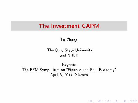
The Investment CAPM

Lu Zhang

The Ohio State Universityand NBER

KeynoteThe EFM Symposium on �Finance and Real Economy�

April 8, 2017, Xiamen

Theme

A new class of capital asset pricing models arises from the �rstprinciple of real investment for individual �rms

SetupA two-period stochastic general equilibrium model

Three de�ning characteristics of neoclassical economics:

Rational expectations

Consumers maximize utility, and �rms maximize market value

Markets clear

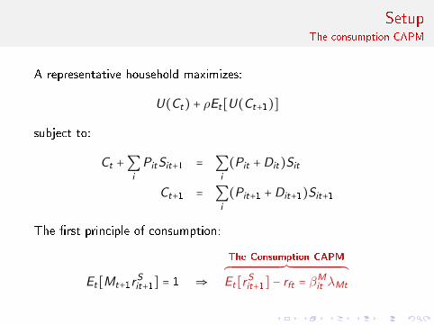
SetupThe consumption CAPM

A representative household maximizes:

U(Ct) + ρEt[U(Ct+1)]

subject to:

Ct +∑i

PitSit+1 = ∑i

(Pit +Dit)Sit

Ct+1 = ∑i

(Pit+1 +Dit+1)Sit+1

The �rst principle of consumption:

Et[Mt+1rSit+1] = 1 ⇒

The Consumption CAPM³¹¹¹¹¹¹¹¹¹¹¹¹¹¹¹¹¹¹¹¹¹¹¹¹¹¹¹¹¹¹¹¹¹¹¹¹¹¹¹¹¹¹¹¹¹¹¹¹¹¹¹¹¹¹¹¹¹¹¹¹¹¹¹¹¹¹·¹¹¹¹¹¹¹¹¹¹¹¹¹¹¹¹¹¹¹¹¹¹¹¹¹¹¹¹¹¹¹¹¹¹¹¹¹¹¹¹¹¹¹¹¹¹¹¹¹¹¹¹¹¹¹¹¹¹¹¹¹¹¹¹¹¹¹µ

Et[rSit+1] − rft = β

Mit λMt

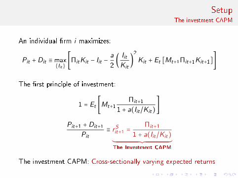
SetupThe investment CAPM

An individual �rm i maximizes:

Pit +Dit ≡ max{Iit}

[ΠitKit − Iit −a

2(IitKit

)

2

Kit + Et [Mt+1Πit+1Kit+1]]

The �rst principle of investment:

1 = Et [Mt+1Πit+1

1 + a(Iit/Kit)]

Pit+1 +Dit+1Pit

≡ rSit+1 =Πit+1

1 + a(Iit/Kit)´¹¹¹¹¹¹¹¹¹¹¹¹¹¹¹¹¹¹¹¹¹¹¹¹¹¹¹¹¹¹¹¹¹¹¹¹¹¹¹¹¹¹¹¹¹¹¹¹¹¹¹¹¹¹¹¹¸¹¹¹¹¹¹¹¹¹¹¹¹¹¹¹¹¹¹¹¹¹¹¹¹¹¹¹¹¹¹¹¹¹¹¹¹¹¹¹¹¹¹¹¹¹¹¹¹¹¹¹¹¹¹¹¹¹¶The Investment CAPM

The investment CAPM: Cross-sectionally varying expected returns

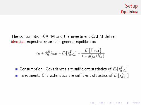
SetupEquilibrium

The consumption CAPM and the investment CAPM deliveridentical expected returns in general equilibrium:

rft + βMit λMt = Et[r

Sit+1] =

Et[Πit+1]1 + a(Iit/Kit)

Consumption: Covariances are su�cient statistics of Et[rSit+1]

Investment: Characteristics are su�cient statistics of Et[rSit+1]

Outline

1 The q-Factor Model

2 The Multiperiod Investment CAPM

3 The Big PictureA Historical PerspectiveComplementarity with the Consumption CAPMThe Aggregation CritiqueAn E�cient Markets CounterrevolutionRevisiting the Joint-Hypothesis Problem

Outline

1 The q-Factor Model

2 The Multiperiod Investment CAPM

3 The Big PictureA Historical PerspectiveComplementarity with the Consumption CAPMThe Aggregation CritiqueAn E�cient Markets CounterrevolutionRevisiting the Joint-Hypothesis Problem

The q-Factor ModelHou, Xue, and Zhang (2015, RFS)

E [rit−rft] = βiMKT E [MKTt]+β

iME E [rME,t]+β

iI/A E [rI/A,t]+βiROE E [rROE,t]

MKTt , rME,t , rI/A,t , and rROE,t are the market, size, investment,and pro�tability (return on equity, ROE) factors, respectively

βiMKT

, βiME, βi

I/A, and βiROE

are factor loadings

The q-factor model largely summarizes the cross section of averagestock returns, capturing most (but not all) anomalies that plaguethe Fama-French 3-factor model and Carhart 4-factor model

The q-Factor ModelIntuition: The investment premium

q and high investment, and high discount rates give rise to low marginal q and low investment. This

discount rate intuition is probably most transparent in the capital budgeting language of Brealey,

Myers, and Allen (2006). In our setting capital is homogeneous, meaning that there is no difference

between project-level costs of capital and firm-level costs of capital. Given expected cash flows,

high costs of capital imply low net present values of new projects and in turn low investment, and

low costs of capital imply high net present values of new projects and in turn high investment.12

Figure 1. The Investment Mechanism

-X-axis: Investment-to-assets

6Y -axis: The discount rate

0

High investment-to-assets firms

SEO firms, IPO firms, convertible bond issuers

High net stock issues firms

Growth firms with low book-to-market

Low market leverage firms

Firms with high long-term prior returns

High accrual firms

High composite issuance firms

���

����

Low investment-to-assets firms

Matching nonissuers

Low net stock issues firms

Value firms with high book-to-market

High market leverage firms

Firms with low long-term prior returns

Low accrual firms

Low composite issuance firms

The negative investment-expected return relation is conditional on expected ROE. Investment

is not disconnected with ROE because more profitable firms tend to invest more than less prof-

itable firms. This conditional relation provides a natural portfolio interpretation of the investment

mechanism. Sorting on net stock issues, composite issuance, book-to-market, and other valuation

ratios is closer to sorting on investment than sorting on expected ROE. Equivalently, these sorts

12The negative investment-discount rate relation has a long tradition in economics. In a world without uncertainty,Fisher (1930) and Fama and Miller (1972, Figure 2.4) show that the interest rate and investment are negativelycorrelated. Intuitively, the investment demand curve is downward sloping. Extending this insight into a world withuncertainty, Cochrane (1991) and Liu, Whited, and Zhang (2009) demonstrate the negative investment-expectedreturn relation in a dynamic setting with constant returns to scale. Carlson, Fisher, and Giammarino (2004)also predict the negative investment-expected return relation. In their real options model expansion options areriskier than assets in place. Investment converts riskier expansion options into less risky assets in place. As such,high-investment firms are less risky and earn lower expected returns than low-investment firms.

23

The q-Factor ModelIntuition: The pro�tability premium

High ROE relative to low investment means high discount rates:

Suppose the discount rates were low

Combined with high ROE, low discount rates would imply highnet present values of new projects and high investment

So discount rates must be high to counteract high ROE toinduce low investment

Price and earnings momentum winners and less �nanciallydistressed �rms have higher ROE and earn higher expected returns

The q-Factor Model�Endorsement� from Fama and French (2015)

The Fama-French 5-factor model:

E [rit − rft] = bi E [MKTt] + si E [SMBt] + hi E [HMLt]

+ri E [RMWt] + ci E [CMAt]

MKTt ,SMBt ,HMLt ,RMWt , and CMAt are the market, size,value, pro�tability, and investment factors, respectively

bi , si ,hi , ri , and ci are factor loadings

The q-Factor ModelPredating the Fama-French 5-factor model by 3�6 years

Neoclassical factors July 2007

An equilibrium three-factor model January 2009Production-based factors April 2009A better three-factor model June 2009

that explains more anomaliesAn alternative three-factor model April 2010, April 2011

Digesting anomalies: An investment approach October 2012 , August 2014

Fama and French (2013): A four-factor model for June 2013the size, value, and pro�tabilitypatterns in stock returns

Fama and French (2014): November 2013 , September 2014

A �ve-factor asset pricing model

The q-Factor ModelA quote from John B. S. Haldane

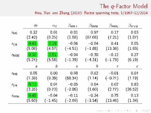
The q-Factor ModelHou, Xue, and Zhang (2016): Factor spanning tests, 1/1967�12/2014

m αC βMKT βSMB βHML βUMD

rME 0.32 0.01 0.01 0.97 0.17 0.03(2.42) (0.25) (1.08) (67.08) (7.21) (1.87)

rI/A 0.43 0.29 −0.06 −0.04 0.41 0.05(5.08) (4.57) (−4.51) (−1.88) (13.36) (1.93)

rROE 0.56 0.51 −0.04 −0.30 −0.12 0.27(5.24) (5.58) (−1.39) (−4.31) (−1.79) (6.19)

a b s h r c

rME 0.05 0.00 0.98 0.02 −0.01 0.04(1.39) (0.39) (68.34) (1.14) (−0.21) (1.19)

rI/A 0.12 0.01 −0.05 0.04 0.07 0.82(3.35) (0.73) (−2.86) (1.60) (2.77) (26.52)

rROE 0.45 −0.04 −0.11 −0.24 0.75 0.13(5.60) (−1.45) (−2.69) (−3.54) (13.46) (1.34)

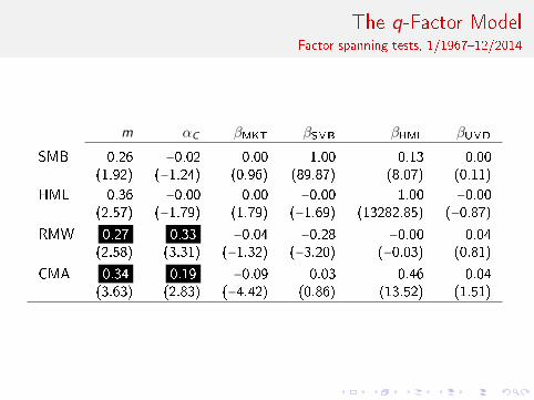
The q-Factor ModelFactor spanning tests, 1/1967�12/2014

m αC βMKT βSMB βHML βUMD

SMB 0.26 −0.02 0.00 1.00 0.13 0.00(1.92) (−1.24) (0.96) (89.87) (8.07) (0.11)

HML 0.36 −0.00 0.00 −0.00 1.00 −0.00(2.57) (−1.79) (1.79) (−1.69) (13282.85) (−0.87)

RMW 0.27 0.33 −0.04 −0.28 −0.00 0.04(2.58) (3.31) (−1.32) (−3.20) (−0.03) (0.81)

CMA 0.34 0.19 −0.09 0.03 0.46 0.04(3.63) (2.83) (−4.42) (0.86) (13.52) (1.51)

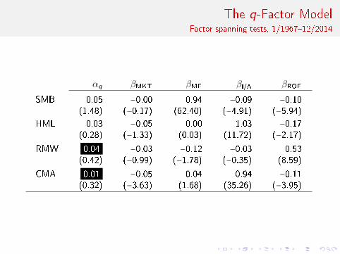
The q-Factor ModelFactor spanning tests, 1/1967�12/2014

αq βMKT βME βI/A βROE

SMB 0.05 −0.00 0.94 −0.09 −0.10(1.48) (−0.17) (62.40) (−4.91) (−5.94)

HML 0.03 −0.05 0.00 1.03 −0.17(0.28) (−1.33) (0.03) (11.72) (−2.17)

RMW 0.04 −0.03 −0.12 −0.03 0.53(0.42) (−0.99) (−1.78) (−0.35) (8.59)

CMA 0.01 −0.05 0.04 0.94 −0.11(0.32) (−3.63) (1.68) (35.26) (−3.95)

Outline

1 The q-Factor Model

2 The Multiperiod Investment CAPM

3 The Big PictureA Historical PerspectiveComplementarity with the Consumption CAPMThe Aggregation CritiqueAn E�cient Markets CounterrevolutionRevisiting the Joint-Hypothesis Problem

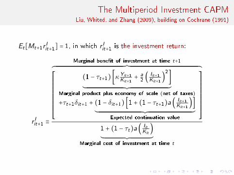
The Multiperiod Investment CAPMLiu, Whited, and Zhang (2009), building on Cochrane (1991)

Et[Mt+1r Iit+1] = 1, in which r Iit+1 is the investment return:

r Iit+1 ≡

Marginal bene�t of investment at time t+1³¹¹¹¹¹¹¹¹¹¹¹¹¹¹¹¹¹¹¹¹¹¹¹¹¹¹¹¹¹¹¹¹¹¹¹¹¹¹¹¹¹¹¹¹¹¹¹¹¹¹¹¹¹¹¹¹¹¹¹¹¹¹¹¹¹¹¹¹¹¹¹¹¹¹¹¹¹¹¹¹¹¹¹¹¹¹¹¹¹¹¹¹¹¹¹¹¹¹¹¹¹¹¹¹¹¹¹¹¹¹¹¹¹¹¹¹¹¹¹¹¹¹¹¹¹¹¹¹¹¹¹¹¹¹¹¹¹¹¹¹¹¹¹¹¹¹¹¹¹¹¹¹¹¹¹¹¹¹¹¹¹¹¹¹¹¹¹¹¹¹¹¹·¹¹¹¹¹¹¹¹¹¹¹¹¹¹¹¹¹¹¹¹¹¹¹¹¹¹¹¹¹¹¹¹¹¹¹¹¹¹¹¹¹¹¹¹¹¹¹¹¹¹¹¹¹¹¹¹¹¹¹¹¹¹¹¹¹¹¹¹¹¹¹¹¹¹¹¹¹¹¹¹¹¹¹¹¹¹¹¹¹¹¹¹¹¹¹¹¹¹¹¹¹¹¹¹¹¹¹¹¹¹¹¹¹¹¹¹¹¹¹¹¹¹¹¹¹¹¹¹¹¹¹¹¹¹¹¹¹¹¹¹¹¹¹¹¹¹¹¹¹¹¹¹¹¹¹¹¹¹¹¹¹¹¹¹¹¹¹¹¹¹¹¹¹µ⎡⎢⎢⎢⎢⎢⎢⎢⎢⎢⎢⎢⎣

(1 − τt+1) [κYit+1Kit+1+ a2(

Iit+1Kit+1

)2

]

´¹¹¹¹¹¹¹¹¹¹¹¹¹¹¹¹¹¹¹¹¹¹¹¹¹¹¹¹¹¹¹¹¹¹¹¹¹¹¹¹¹¹¹¹¹¹¹¹¹¹¹¹¹¹¹¹¹¹¹¹¹¹¹¹¹¹¹¹¹¹¹¹¹¹¹¹¹¹¹¹¹¹¹¹¹¹¹¹¹¹¹¹¹¹¸¹¹¹¹¹¹¹¹¹¹¹¹¹¹¹¹¹¹¹¹¹¹¹¹¹¹¹¹¹¹¹¹¹¹¹¹¹¹¹¹¹¹¹¹¹¹¹¹¹¹¹¹¹¹¹¹¹¹¹¹¹¹¹¹¹¹¹¹¹¹¹¹¹¹¹¹¹¹¹¹¹¹¹¹¹¹¹¹¹¹¹¹¹¹¹¶Marginal product plus economy of scale (net of taxes)+τt+1δit+1 + (1 − δit+1) [1 + (1 − τt+1)a ( Iit+1

Kit+1)]

´¹¹¹¹¹¹¹¹¹¹¹¹¹¹¹¹¹¹¹¹¹¹¹¹¹¹¹¹¹¹¹¹¹¹¹¹¹¹¹¹¹¹¹¹¹¹¹¹¹¹¹¹¹¹¹¹¹¹¹¹¹¹¹¹¹¹¹¹¹¹¹¹¹¹¹¹¹¹¹¹¹¹¹¹¹¹¹¹¹¹¹¹¹¹¹¹¹¹¹¹¹¹¹¹¹¹¹¹¹¸¹¹¹¹¹¹¹¹¹¹¹¹¹¹¹¹¹¹¹¹¹¹¹¹¹¹¹¹¹¹¹¹¹¹¹¹¹¹¹¹¹¹¹¹¹¹¹¹¹¹¹¹¹¹¹¹¹¹¹¹¹¹¹¹¹¹¹¹¹¹¹¹¹¹¹¹¹¹¹¹¹¹¹¹¹¹¹¹¹¹¹¹¹¹¹¹¹¹¹¹¹¹¹¹¹¹¹¹¹¹¶Expected continuation value

⎤⎥⎥⎥⎥⎥⎥⎥⎥⎥⎥⎥⎦

1 + (1 − τt)a (IitKit

)

´¹¹¹¹¹¹¹¹¹¹¹¹¹¹¹¹¹¹¹¹¹¹¹¹¹¹¹¹¹¹¹¹¹¹¹¹¹¹¹¹¹¹¹¹¹¹¹¹¸¹¹¹¹¹¹¹¹¹¹¹¹¹¹¹¹¹¹¹¹¹¹¹¹¹¹¹¹¹¹¹¹¹¹¹¹¹¹¹¹¹¹¹¹¹¹¹¹¹¶Marginal cost of investment at time t

The Multiperiod Investment CAPMThe �rst principle of investment

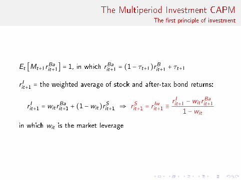
Et [Mt+1rBait+1] = 1, in which rBait+1 = (1 − τt+1)rBit+1 + τt+1

r Iit+1 = the weighted average of stock and after-tax bond returns:

r Iit+1 = witrBait+1 + (1 −wit)r

Sit+1 ⇒ rSit+1 = r Iwit+1 ≡

r Iit+1 −witrBait+1

1 −wit

in which wit is the market leverage

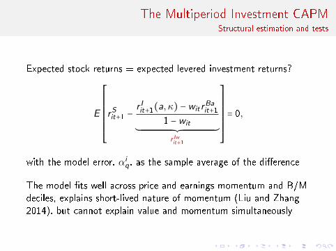
The Multiperiod Investment CAPMStructural estimation and tests

Expected stock returns = expected levered investment returns?

E

⎡⎢⎢⎢⎢⎢⎢⎢⎢⎢⎣

rSit+1 −r Iit+1(a, κ) −witr

Bait+1

1 −wit´¹¹¹¹¹¹¹¹¹¹¹¹¹¹¹¹¹¹¹¹¹¹¹¹¹¹¹¹¹¹¹¹¹¹¹¹¹¹¹¹¹¹¹¹¹¹¹¹¹¹¹¹¹¹¹¹¸¹¹¹¹¹¹¹¹¹¹¹¹¹¹¹¹¹¹¹¹¹¹¹¹¹¹¹¹¹¹¹¹¹¹¹¹¹¹¹¹¹¹¹¹¹¹¹¹¹¹¹¹¹¹¹¹¶

r Iwit+1

⎤⎥⎥⎥⎥⎥⎥⎥⎥⎥⎦

= 0,

with the model error, αiq, as the sample average of the di�erence

The model �ts well across price and earnings momentum and B/Mdeciles, explains short-lived nature of momentum (Liu and Zhang2014), but cannot explain value and momentum simultaneously

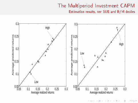
The Multiperiod Investment CAPMEstimation results, ten SUE and B/M deciles

0.05 0.1 0.15 0.2 0.25 0.30.05

0.1

0.15

0.2

0.25

0.3

Average realized returns

Ave

rag

e p

red

icte

d r

etu

rns

Low

High

0.05 0.1 0.15 0.2 0.25 0.30.05

0.1

0.15

0.2

0.25

0.3

Average realized returns

Avera

ge p

redic

ted r

etu

rns

Low

High

Outline

1 The q-Factor Model

2 The Multiperiod Investment CAPM

3 The Big PictureA Historical PerspectiveComplementarity with the Consumption CAPMThe Aggregation CritiqueAn E�cient Markets CounterrevolutionRevisiting the Joint-Hypothesis Problem

The Big PictureA historical perspective: Böhm-Bawert (1891, The positive theory of capital)

1st generation Austrian Schooleconomists, with Carl Mengerand Friedrich von Wieser

Why the interest rate > 0?

1. The falling marginal utility ofincome over time

2. Consumers tend tounderestimate future needs

3. �Roundabout� production:Production per worker rises withthe production length

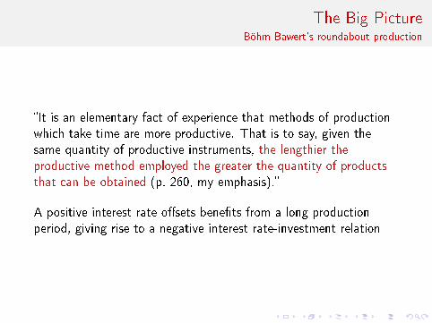
The Big PictureBöhm-Bawert's roundabout production

�It is an elementary fact of experience that methods of productionwhich take time are more productive. That is to say, given thesame quantity of productive instruments, the lengthier theproductive method employed the greater the quantity of productsthat can be obtained (p. 260, my emphasis).�

A positive interest rate o�sets bene�ts from a long productionperiod, giving rise to a negative interest rate-investment relation

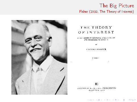
The Big PictureFisher (1930, The Theory of Interest)

The Big PictureThe Fisherian equilibrium

up in the production process. This effect is exactly the negative relation between real investment

and the discount rate (Figure 1), albeit without uncertainty.

Fisher (1930) studies the economic determinants of the real interest rate by constructing the

first general equilibrium model with both intertemporal exchange and production. His model also

shows the Fisher Separation Theorem, which justifies the maximization of the present value as the

objective of the firm, without any direct dependence on shareholder preferences. Figure 6, which

is adapted from Chart 38 in Fisher (p. 271), shows the key insights.

Figure 6. The Fisherian Equilibrium

✲C0

✻C1

0

tQ

tP❏❏❏❏❏❏❏❏❏❏❏❏❏❏❏❏❏❏❏❏❏❏❏❏❏

tO

K0

❏❏❏❏❏❏❏❏❏❏❏❏❏❏❏❏❏❏

(1 + r)K0

U0

U1

K1

In the figure, the horizontal axis labeled C0 represents consumption in date 0, and the vertical

axis C1 represents consumption in date 1. Endowed with an amount of resources, K0, in date 0,

the agent’s problem is to choose an optimal time pattern of consumption. The agent’s preferences

are represented by indifference curves, such as U0 and U1. There are two available ways to transfer

81

The �rst general equilibriummodel with both intertemporalconsumption and production

Fisher Separation Theorem:Maximizing the present value offree cash �ows as the objectiveof the �rm, without anydependence on shareholderpreferences

The Big PictureJack Hirshleifer's (1958, 1965, 1966, 1970) seminal work

Revives and extends Fisher's(1930) general equilibriumanalysis to uncertainty

A pioneer in applying theArrow-Debreu state-preferenceapproach in �nance, includingcapital budgeting and capitalstructure

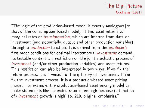
The Big PictureCochrane (1991)

�The logic of the production-based model is exactly analogous [tothat of the consumption-based model]. It ties asset returns tomarginal rates of transformation, which are inferred from data oninvestment (and potentially, output and other production variables)through a production function. It is derived from the producer's

�rst order conditions for optimal intertemporal investment demand.Its testable content is a restriction on the joint stochastic process ofinvestment (and/or other production variables) and asset returns.This restriction can also be interpreted in two ways. If we �x thereturn process, it is a version of the q theory of investment. If we�x the investment process, it is a production-based asset pricingmodel. For example, the production-based asset pricing model canmake statements like `expected returns are high because (a functionof) investment growth is high' (p. 210, original emphasis).�

The Big PictureModern asset pricing thoroughly dominated by the consumption CAPM

In hindsight, thanks to Arrow-Debreu, asset pricing theory is justthe standard price theory extended to uncertainty and over time

Fisher (1930) did the extension over time; Debreu (1959),Arrow (1964), and J. Hirshleifer (1970) did uncertainty

Asset pricing theorists, led by Markowitz (1952), started withinvestors' problem under uncertainty, and never looked back

Markowitz (1952); Roy (1952)

Treynor (1962); Sharpe (1964); Lintner (1965); Mossin (1966)

Merton (1973); Long (1974)

Empirical work reinforced the investors-centered CAPM, by favoringthe mean variance approach over the state-preference approach

Fama and Miller (1972); Fama (1976)

The Big PictureBöhm-Bawert's, Fisher's, and J. Hirshleifer's investment opportunity approach to the

interest rate/discount rate all disappeared from modern asset pricing

Rubinstein (1976); Lucas(1978); Breeden (1979)

Hansen and Singleton (1982);Breeden, Gibbons, andLitzenberger (1989)

Cochrane (2005): �All assetpricing models amount toalternative ways of connectingthe stochastic discount factor todata (p. 7, original emphasis).�

Bodie, Kane, and Marcus; Berkand DeMarzo

The Big PictureInspired by Cochrane (1991), I recognize in Zhang (2005a) that the neoclassical q-theory

of investment allows a di�erent reduction of the general equilibrium problem

NBER WORKING PAPER SERIES

ANOMALIES

Lu Zhang

Working Paper 11322http://www.nber.org/papers/w11322

NATIONAL BUREAU OF ECONOMIC RESEARCH1050 Massachusetts Avenue

Cambridge, MA 02138May 2005

I acknowledge helpful comments from Rui Albuquerque, Yigit Atilgan, Jonathan Berk, Mike Barclay, MarkBils, Robert Bloom eld, Murray Carlson, Huafeng Chen, John Cochrane, Evan Dudley, Joao Gomes, JeremyGreenwood, Zvi Hercowitz, Leonid Kogan, Pete Kyle, Xuenan Li, Laura Liu, John Long, Lionel McKenzie,Roni Michaely, Sabatino Silveri, Bill Schwert, TaoWang, JerryWarner, DavidWeinbaum, Joanna Wu, MikeYang, and seminar participants at Haas School of Business at University of California at Berkeley, SloanSchool of Management at Massachusetts Institute of Technology, Johnson School of Management at CornellUniversity, Simon School of Business and Department of Economics at University of Rochester, NBERAsset Pricing meeting, and Utah Winter Finance Conference. The usual disclaimer applies. The viewsexpressed herein are those of the author(s) and do not necessarily reflect the views of the National Bureauof Economic Research.

©2005 by Lu Zhang. All rights reserved. Short sections of text, not to exceed two paragraphs, may be quotedwithout explicit permission provided that full credit, including © notice, is given to the source.

I was intrigued by anomalies butdisturbed by behavioral �nance

The investment CAPMexpresses expected returns interms of �rm characteristicswithout any dependence onshareholder preferences, thelatest incarnation of FisherSeparation Theorem

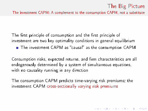
The Big PictureThe investment CAPM: A complement to the consumption CAPM, not a substitute

The �rst principle of consumption and the �rst principle ofinvestment are two key optimality conditions in general equilibrium

The investment CAPM as �causal� as the consumption CAPM

Consumption risks, expected returns, and �rm characteristics are allendogenously determined by a system of simultaneous equations,with no causality running in any direction

The consumption CAPM predicts time-varying risk premiums; theinvestment CAPM cross-sectionally varying risk premiums

The Big PictureMarshall's �scissors:� Marshall (1890, Principles of Economics)

The Big PictureMarshall's �scissors:� History tends to repeat itself?

Ricardo and Mill: Costs of production determine value, but Jevons,Menger, and Walras: Marginal utility determines value

The water versus diamond example

�We might as reasonably dispute whether it is the upper or underblade of a pair of scissors that cuts a piece of paper, as whethervalue is governed by utility or costs of production. It is true thatwhen one blade is held still, and the cutting is a�ected by movingthe other, we may say with careless brevity that the cutting is doneby the second; but the statement is not strictly accurate, and is tobe excused only so long as it claims to be merely a popular and nota strictly scienti�c account of what happens (Marshall 1890 [1961,9th edition, p. 348], my emphasis).�

The Big PictureThe ubiquitous representative investor

If the investment CAPM and the consumption CAPM arecomplementary, why does the former perform better in the data?

What explains the empirical failure of the consumption CAPM?

Most consumption CAPM studies assume a representative investor

The Sonnenschein-Mantel-Debreu theorem in general equilibriumtheory: The aggregate excess demand function is not restricted bythe standard rationality assumption on individual demands

The Big PictureKirman's (1992) four objections to a representative investor

Individual maximization does not imply collective rationality;collective maximization does not imply individual rationality

The response of the representative to a parameter changemight not be the same as the aggregate response of individuals

It is possible for the representative to exhibit preferenceorderings that are opposite to all the individuals'.

The aggregate behavior of rational individuals might exhibitcomplicated dynamics, and imposing these dynamics on oneindividual can lead to unnatural characteristics of the individual

The Big PictureA case in point

Is it possible to assign rational preferences to �the representativevoter� in the U.S. that picked Trump after Obama?

Insisting on assigning would yield highly irrational preferences

Analogously, assigning irrational preferences on the representativeinvestor is not particularly illuminating

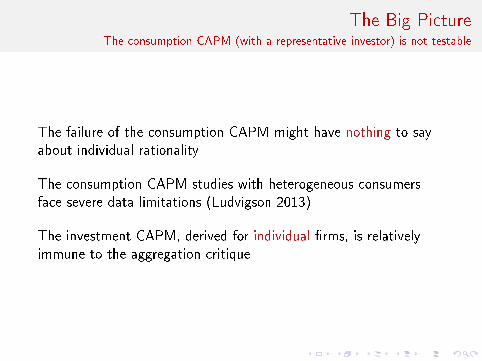
The Big PictureThe consumption CAPM (with a representative investor) is not testable

The failure of the consumption CAPM might have nothing to sayabout individual rationality

The consumption CAPM studies with heterogeneous consumersface severe data limitations (Ludvigson 2013)

The investment CAPM, derived for individual �rms, is relativelyimmune to the aggregation critique

The Big PictureAn e�cient markets counterrevolution

The investment CAPM o�ers a powerful defense of e�cient markets

The Big PictureA �dark age� of �nance

�Research in experimental psychology suggests that, in violation ofBayes' rule, most people tend to `overreact' to unexpected anddramatic news events. This study of market e�ciency investigateswhether such behavior a�ects stock prices. The empirical evidence,based on CRSP monthly return data, is consistent with theoverreaction hypothesis. Substantial weak form marketine�ciencies are discovered (De Bondt-Thaler 1985, p. 793).�

�[It] is possible that the market underreacts to information abouttheir short-term prospects of �rms but overreacts to informationabout their long-term prospects. This is plausible given that thenature of the information available about a �rm's short-termprospects, such as earnings forecasts, is di�erent from the nature ofthe more ambiguous information that is used by investors to assessa �rm's longer-term prospects (Jegadeesh-Titman 1993, p. 90).�

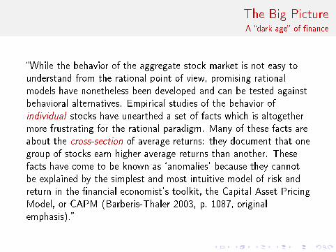
The Big PictureA �dark age� of �nance

�While the behavior of the aggregate stock market is not easy tounderstand from the rational point of view, promising rationalmodels have nonetheless been developed and can be tested againstbehavioral alternatives. Empirical studies of the behavior ofindividual stocks have unearthed a set of facts which is altogethermore frustrating for the rational paradigm. Many of these facts areabout the cross-section of average returns: they document that onegroup of stocks earn higher average returns than another. Thesefacts have come to be known as `anomalies' because they cannotbe explained by the simplest and most intuitive model of risk andreturn in the �nancial economist's toolkit, the Capital Asset PricingModel, or CAPM (Barberis-Thaler 2003, p. 1087, originalemphasis).�

The Big PictureA defense of e�cient markets

The argument for ine�cient markets based on the failure of theCAPM represents, to paraphrase Shiller (1984), �one of the mostremarkable errors in the history of economic thought�

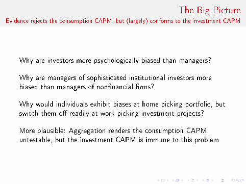
The Big PictureEvidence rejects the consumption CAPM, but (largely) conforms to the investment CAPM

Why are investors more psychologically biased than managers?

Why are managers of sophisticated institutional investors morebiased than managers of non�nancial �rms?

Why would individuals exhibit biases at home picking portfolio, butswitch them o� readily at work picking investment projects?

More plausible: Aggregation renders the consumption CAPMuntestable, but the investment CAPM is immune to this problem

The Big PictureSome evidence on the cross-country variation of anomalies

The investment e�ect is stronger in developed than emergingmarkets, as shown in Titman, Wei, and Xie (2013)

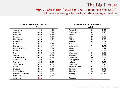
The Big PictureGri�n, Ji, and Martin (2003) and Chui, Titman, and Wei (2010):

Momentum stronger in developed than emerging markets

Panel A: Developed markets Panel B: Emerging markets

WML t WML t

Australia 1.08 4.76 Argentina 0.08 0.12Austria 0.63 2.70 Bangladesh 1.68 2.75Belgium 0.89 5.50 Brazil 0.46 0.96Canada 1.35 6.29 Chile 0.99 3.60Denmark 0.96 4.29 China 0.26 0.92Finland 0.98 2.62 Greece 0.59 1.49France 0.94 4.68 India 1.14 2.91Germany 0.99 4.41 Indonesia 0.14 0.30Hong Kong 0.77 3.18 Israel 0.32 1.19Ireland 0.88 3.06 Korea −0.34 −0.81Italy 0.90 4.47 Malaysia 0.10 0.26Japan −0.04 −0.18 Mexico 0.69 2.00Netherlands 0.83 4.40 Pakistan 0.46 1.05New Zealand 1.58 5.01 Philippines 0.37 0.68Norway 1.05 3.77 Poland 1.76 3.33Singapore 0.14 0.47 Portugal 0.31 0.93Spain 0.63 2.24 South Africa 0.94 3.29Sweden 0.71 2.27 Taiwan −0.20 −0.48Switzerland 0.82 4.39 Thailand 0.48 1.10United Kingdom 1.13 7.08 Turkey −0.41 −0.96United States 0.79 3.44Average 0.86 Average 0.49

The Big PictureCross-country variation of anomalies, explanations?

Why are U.S. investors more biased than Chinese investors? Whydoes the U.S. have higher limits to arbitrage than China?

Behavioral �nance relies on dysfunctional, ine�cient markets forbiases and limits to arbitrage to work, contradicting the evidence

The investment CAPM relies on well functioning, e�cient marketsfor its mechanisms to work, consistent with the evidence

The Big PictureA tribute to Fama and French (1993)

The three-factor model has served its historical purpose, admirably.

Filled the vacuum left by the CAPM after its rejection in Fama andFrench (1992) as the workhorse model in e�cient markets

Alas, ad hoc, vulnerable to the data mining critique

The relative distress interpretation refuted by the distress anomaly

The risk factors interpretation in the ICAPM-APT unconvincing

The Big PictureInterpreting factors: The investment CAPM perspective

Characteristics-based factor models as linear approximations to theinvestment CAPM

The investment CAPM predicts all kinds of relations betweencharacteristics and expected returns:

Characteristics forecasting returns not necessarily mispricing

No need to insist on risk factors to defend e�cient markets

Time series and cross-sectional regressions are two di�erent ways ofsummarizing correlations, largely equivalent in economic terms

The Big PictureThe �risk doctrine�

�Most of the available work is based only on the assumption thatthe conditions of market equilibrium can (somehow) be stated interms of expected returns. In general terms, like the two parametermodel such theories would posit that conditional on some relevantinformation set, the equilibrium expected return on a security is afunction of its `risk.' And di�erent theories would di�er primarily inhow `risk' is de�ned (Fama 1970, p. 384, my emphasis).�

The Big PictureChallenging the �risk doctrine�

Only describes the consumption CAPM

Does not apply to the investment CAPM, in which characteristicsare su�cient statistics for expected returns, and aftercharacteristics are controlled for, risks should not matter

Neither risks nor characteristics �determine� expected returns

Risks as driving forces: A relic and illusion from the CAPM

The Big PictureMoving from the consumption CAPM to the investment CAPM

�[The] really pressing problems, e.g., a cure for cancer and thedesign of a lasting peace, are often not puzzles at all, largelybecause they may not have any solution. Consider the jigsaw puzzlewhose pieces are selected at random from each of two di�erentpuzzle boxes. Since that problem is likely to defy (though it mightnot) even the most ingenious of men, it cannot serve as a test ofskill. In solution in any usual sense, it is not a puzzle at all.Though intrinsic value is no criterion for a puzzle, the assuredexistence of a solution is (Kuhn 1962, p. 36�37, my emphasis).�

Conclusion

Like any prices, asset prices are equilibrated by supply and demand

The consumption CAPM and behavioral �nance, both of which aredemand-based, cannot possibly be the whole story

Anomalies doom the consumption CAPM, but behavioral �nance isnot the answer; the investment CAPM as a new paradigm

Conclusion

Make Finance Great Again!

,