RESEARCH ARTICLE

The use of mesoscale eddies by juvenile

loggerhead sea turtles (Caretta caretta) in the

southwestern Atlantic

Peter Gaube1¤*, Caren Barcelo2, Dennis J. McGillicuddy, Jr.1, Andres Domingo3,

Philip Miller4, Bruno Giffoni5, Neca Marcovaldi5, Yonat Swimmer6

1 Department of Applied Ocean Physics and Engineering, Woods Hole Oceanographic Institution, Woods

Hole, Massachusetts, United States of America, 2 College of Earth, Ocean and Atmospheric Sciences,

Oregon State University, Corvallis, Oregon, United States of America, 3 Direccion Nacional de Recursos

Acuaticos, Montevideo, Uruguay, 4 Centro de Investigacion y Conservacion Marina (CICMAR), El Pinar,

Canelones, Uruguay, 5 Projecto TAMAR, Fundacão Pro Tamar / ICMBio, Salvador, Bahia, Brazil, 6 NOAA

Fisheries, Long Beach, California, United States of America

¤ Current address: Air-Sea Interaction and Remote Sensing Department, Applied Physics Laboratory—

University of Washington, Seattle, Washington, United States of America

* pgaube@apl.washington.edu

Abstract

Marine animals, such as turtles, seabirds and pelagic fishes, are observed to travel and con-

gregate around eddies in the open ocean. Mesoscale eddies, large swirling ocean vortices

with radius scales of approximately 50–100 km, provide environmental variability that can

structure these populations. In this study, we investigate the use of mesoscale eddies by 24

individual juvenile loggerhead sea turtles (Caretta caretta) in the Brazil-Malvinas Confluence

region. The influence of eddies on turtles is assessed by collocating the turtle trajectories to

the tracks of mesoscale eddies identified in maps of sea level anomaly. Juvenile loggerhead

sea turtles are significantly more likely to be located in the interiors of anticyclones in this

region. The distribution of surface drifters in eddy interiors reveals no significant association

with the interiors of cyclones or anticyclones, suggesting higher prevalence of turtles in anti-

cyclones is a result of their behavior. In the southern portion of the Brazil-Malvinas Conflu-

ence region, turtle swimming speed is significantly slower in the interiors of anticyclones,

when compared to the periphery, suggesting that these turtles are possibly feeding on prey

items associated with anomalously low near-surface chlorophyll concentrations observed in

those features.

Introduction

Mesoscale eddies have been identified as “hot spots” of biological activity, spanning trophic

levels from primary producers [1–4] to zooplankton and small fish [5], up to large pelagic fish

[6]. Recent advances in satellite oceanography have allowed the automated identification and

tracking of mesoscale ocean eddies globally [7]. These advances in our ability to observe and

track eddies has enabled us to analyze their impact on marine biota, revealing rich regional

variability in how eddies influence near-surface chlorophyll (CHL) distributions [8, 9] and

structure populations of animals (e.g., [10]).

PLOS ONE | DOI:10.1371/journal.pone.0172839 March 1, 2017 1 / 19

a1111111111

a1111111111

a1111111111

a1111111111

a1111111111

OPENACCESS

Citation: Gaube P, Barcelo C, McGillicuddy DJ, Jr.,

Domingo A, Miller P, Giffoni B, et al. (2017) The

use of mesoscale eddies by juvenile loggerhead

sea turtles (Caretta caretta) in the southwestern

Atlantic. PLoS ONE 12(3): e0172839. doi:10.1371/

journal.pone.0172839

Editor: Elliott Lee Hazen, University of California

Santa Cruz, UNITED STATES

Received: July 13, 2016

Accepted: February 10, 2017

Published: March 1, 2017

Copyright: This is an open access article, free of all

copyright, and may be freely reproduced,

distributed, transmitted, modified, built upon, or

otherwise used by anyone for any lawful purpose.

The work is made available under the Creative

Commons CC0 public domain dedication.

Data Availability Statement: This work uses a

combination of primary and third-party data. The

turtle location data are the only primary data and

have been made available as a Supporting

Information file. The third-party data can all be

freely-accessed via the URLs listed within the

manuscript. For more information: Contact person

for Uruguay and Brazil turtle tracking data: Yonat

Swimmer (yonat.swimmer@noaa.gov); Contact for

eddy analysis and satellite data: Peter Gaube

(pgaube@apl.washington.edu).

Furthering our understanding of how ocean current influence the distribution of marine

animals, however, remains a major challenge in the field of pelagic ecology. Significant progress

can now be gained via the development of analysis techniques that aim to elucidate how animals

use oceanographic features, such as eddies and fronts, which has only recently been possible

with the advent of mesoscale feature tracking techniques described above. For example, in the

Atlantic Ocean, Mansfield et al. [11] affixed small solar powered satellite transmitters to neonate

logger head turtles (carapace length 11–18 cm) observing migrations that spanned thousands of

kilometers with individuals spending on average nearly 70% of their time swimming in meso-

scale eddies shed from the Gulf Stream. In the northwestern Pacific, along the Kuroshio Exten-

sion, Polovina et al. [12] observed juvenile loggerhead turtles interacting with the peripheries of

eddies, at times swimming against the prevailing current. The authors suggested that the forag-

ing advantage associated with eddy currents exceed the energetic demand associated with swim-

ming against the current. A series of studies of the post nesting migration of loggerhead sea

turtles revealed that in the Gulf of Mexico, North Pacific, and North Atlantic, turtles displayed a

preference for the periphery of open-ocean eddies, suggesting that these turtles were foraging in

those areas [13, 14]. The aforementioned studies were conducted in a turtle-centric frame of ref-

erence, collocating satellite observations to the turtle trajectories. In a region of high abundance

between Taiwan and China (referred to as a turtle “hotspot”), Kobayashi et al. [10] analyzed the

trajectories of 34 non-reproductive loggerhead sea turtles by collocating their locations to both

the centers and peripheries of mesoscale eddies. Their study revealed that the turtles avoided

the peripheries of cyclonic eddies, in contrast to what was observed in other regions.

The studies described above conclude that turtles use different parts of eddies depending

on their geographic location or life stage. In this study, we investigate the use of eddies by juve-

nile loggerhead sea turtles in the Brazil-Malvinas Confluence (BMC) region by collocating the

daily positions of 24 individual turtles with eddies identified and tracked in maps of sea level

anomaly (SLA). Our investigation aims to: 1) characterize the distributions of eddy polarity,

amplitude, radius, and lifetime in the BMC region; 2) investigate the influence of eddies on

CHL and sea surface temperature (SST) in this region; and 3) compare the distribution of tur-

tles relative to passive Lagrangian drifters in regard to eddies, which has been shown to allow

for the determination of the relative roles of active changes in turtle swimming behavior to

passive advection of turtles by the ambient ocean surface currents [15]. Specifically, we seek to

understand if loggerhead turtles in this region are modifying their behavior to interact with

and remain in eddies, or whether their distribution is the result of the passive advection.

Methods

Sea level anomaly, geostrophic velocities and rddy identification

This investigation of the use of mesoscale eddies by juvenile loggerhead sea turtles was based

on eddies with lifetimes of 12 weeks (84 days) and longer that have been identified and tracked

based on their signatures in SLA [7]. The altimeter-tracked eddy dataset used in this analysis is

available online at http://cioss.coas.oregonstate.edu/eddies. The SLA fields were obtained from

Collecte Localis Satellites (CLS/AVISO, http://www.aviso.altimetry.fr) at 7-day intervals on a 1/

4˚ latitude by 1/4˚ longitude grid. Prior to the identification and tracking of mesoscale eddies,

the SLA fields were high-pass filtered to remove the effects of seasonal heating and cooling [7].

In order to infer swimming behavior of the turtles (see 2.2 below), geostrophic current

velocities were estimated by centered finite differencing of the SLA fields:

ug ¼ �gf@SLA

@yð1Þ

Turtles in eddies

PLOS ONE | DOI:10.1371/journal.pone.0172839 March 1, 2017 2 / 19

Funding: Support was provided by: Woods Hole

Oceanographic Institution [www.whoi.edu] to PG;

National Aeronautics and Space Administration

[www.nasa.gov] NNX13AE47G to PG and DJM;

and National Science Foundation [www.nsf.gov]

1314109 to CB.

Competing interests: The authors have declared

that no competing interests exist.

vg ¼gf@SLA

@xð2Þ

where g is the gravational constant and f = 2O sin F is the Coriolis parameter for latitude F

and Earth rotation rate O and x and y are the zonal and meridional coordinate, respectively.

As described in detail in Appendix B of [7], mesoscale eddies were identified and tracked

based on closed contours of SLA. The eddy amplitude at each weekly time step along its trajec-

tory was defined as the difference between the SLA at the eddy centroid and around the outer-

most closed contour of SLA. The characteristic rotational speed of each eddy (U) was defined

as the average geostrophic speed along the SLA contour around which U is maximum, and

was computed at each point along the eddy trajectory. The horizontal speed-based radius scale

of the eddy (Ls) was defined to be the radius of a circle with area equal to that enclosed by this

SLA contour. The eddy propagation speed was estimated at each point along the eddy trajec-

tory from centered differences of the x and y coordinates of successive eddy SLA centroid

locations.

In order to avoid the complexities of coastal habitats, we considered areas with water depth

in excess 3,000 m, as defined by the National Oceanic and Atmospheric Administration

(NOAA), National Geophysical Data Center, 2-minute Gridded Global Relief Data (ETO-

PO2v2, https://www.ngdc.noaa.gov/mgg/global/etopo2.html) (Fig 1B).

Tracking turtles

Scientific observers of PNOFA-DINARA (the Uruguayan National Program of Scientific

Observers Onboard the Tuna Fleet) [16, 17] and Projeto TAMAR-ICMBio (the national Bra-

zilian sea turtle conservation program) [18] deployed satellite transmitters on loggerhead sea

turtles incidentally captured in Brazilian and Uruguayan pelagic long-line fisheries operating

in the southwestern Atlantic Ocean between July of 2006 and November of 2009. The turtle

trajectories used in this study span a 5-year period between July 2006 and December 2011(Fig

1E) and are available in S1 File.

As described in [16] satellite transmitters were attached to the turtles on the second central

carapacial scute using quick-drying two-part epoxies, PoxipolTM (Uruguay) and DurepoxiTM(Brazil), and allowed to dry for 30 minutes to one hour on deck before release. A total of 24

tracked loggerheads with mean curved carapace length of 61.8 ± 6.9 cm (range: 49 to 83 cm,

see Table 1 of [15]) that transmitted more than 30 days are included in this study. ARGOS-

linked Telonics (Mesa, AZ, USA) platform transmitter terminals (PTTs), models ST-18 and

ST-20, were attached to 4 and 5 turtles, respectively, on Brazilian vessels. ARGOS-linked Wild-life Computers (Redmond, WA, USA) PTTs, models SPLASH and SPOT 5, were attached to 5

and 10 turtles, respectively, on Uruguayan vessels. See [16] for further turtle tracking details.

The first ten days (3% of total points) of tracking data were excluded from each turtle in

order to avoid including immediate post-release behavior that may have been affected by the

capture event. We only considered individual turtle locations with ARGOS estimated errors of

<1500 m of the tag’s actual position (location classes 1–3, ARGOS 2008). Tracking data were

downloaded and filtered using the Satellite Tracking and Analyst Tool [19]. We used single

daily locations in order to reduce spatial autocorrelation [20–22]. Only daily turtle locations

that had observed turtle propagation speed of< 5 km h-1 from one day to the next are retained

[20, 21]. The speed-based thresholding results in the removal of 1% of the total turtle locations.

Turtle trajectories represent the summation of both turtle swimming behavior and ocean

surface currents [23]. The total vector turtle velocity (ut, vt) was defined as the velocity

Turtles in eddies

PLOS ONE | DOI:10.1371/journal.pone.0172839 March 1, 2017 3 / 19

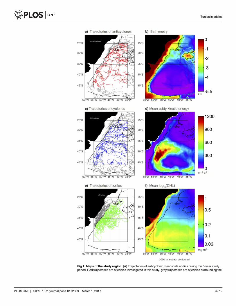
Fig 1. Maps of the study region. (A) Trajectories of anticyclonic mesoscale eddies during the 5-year study

period. Red trajectories are of eddies investigated in this study, grey trajectories are of eddies surrounding the

Turtles in eddies

PLOS ONE | DOI:10.1371/journal.pone.0172839 March 1, 2017 4 / 19

components estimated from the distance an individual turtle travels between successive daily

locations. Similar to Putman and Mansfield (24), the turtle swimming speed Vs was defined as

Vs ¼

ffiffiffiffiffiffiffiffiffiffiffiffiffiffiffiffiffiffiffiffiffiffiffiffiffiffiffiffiffiffiffiffiffiffiffiffiffiffiffiffiffiffiffiffi

ðut � ugÞ2þ ðvt � vgÞ

2

q

: ð3Þ

This formulation assumes that the fluid motions are purely geostrophic. Of course there are

departures from geostrophy, but in the open ocean ageostrophic flows tend to be much weaker

than the geostrophic component. In the near-surface region where the turtles reside, the larg-

est source of ageostrophic flow is wind-driven motion. Across the BMC region, the long-term

average wind-driven surface currents estimated from scatterometer data, as described in [8],

range from 8 cm s-1 to 16 cm s-1 (not shown) and the wind direction is highly variable (see Fig

12 in [8]). Typical geostrophic flows are several times larger and more persistent in time, thus

the wind-driven component can be thought of as high-frequency noise on the signal of inter-

est. Moreover, the average magnitude of the turtle movement vectors is ~70 cm s-1, suggesting

that to first order the approximation in Eq (3) is valid: Vs is a function of turtle behavior, and

not passive advection by wind-driven currents.

Drifters

The surface drifter data set was acquired from NOAA’s Atlantic Oceanographic and Meteoro-

logical Laboratory (ftp://ftp.aoml.noaa.gov/pub/phod/buoydata/hourly_product). A total of 282

drifters were extracted within the study region during the 5-year study period. Drifters are

equipped with an approximately 5m long holey-sock drogue that is centered at 15m which

allows the drifter to follow near-surface currents with minimal wind slip. Zonal and meridio-

nal root-mean-square errors in the satellite location fix are 630 m and 270 m, respectively (see

overview of the global drifter program by [25]). Poor ARGOS locations were removed from the

dataset and the trajectory of each drifter was created by optimal interpolation at uniform 6hour intervals following AOML procedures [26]. The four-times-a-day drifter locations were

then averaged to once-per-day to match the temporal resolution of the turtle tracks.

Near-surface chlorophyll concentration

This study uses the merged SeaWiFS, MODIS-Aqua and MERIS ocean color measurements.

Near-surface chlorophyll pigment concentrations (CHL) were estimated from ocean color

measurements using the Garver-Siegel-Maritorena (GSM) semi-analytical ocean color algo-

rithm [27–29] with data available at ftp://ftp.oceancolor.ucsb.edu//pub/org/oceancolor/MEaSUREs/MergedSAM/. The detailed description of the processing details of the CHL obser-

vations can be found in [30]. Chlorophyll anomaly fields (CHL’) were defined as:

CHL0 ¼ CHL � hCHLi ð4Þ

where hCHLi denotes 6˚ × 6˚ spatially smoothed fields that are removed from the total fields

to create the anomalies.

Ambient CHL varies by more than an order of magnitude over the region of interest (Fig

1F), resulting in inhomogeneities of the CHL anomalies. To help mitigate the effects of

region of interest, but not used in the analysis. (B) Bathymetric map of the study region. (C) Same as panel a,

but for cyclonic eddies. (D) Mean eddy kinetic energy from satellite SLA observations. (E) Tracks of the 24

turtles. Grey trajectories indicate when the turtles were observed to be shallower than 3,000m, and were

excluded from the analysis here. (F) Mean of the log10 transformed CHL. The 3,000 m isobath is contoured in

all panels.

doi:10.1371/journal.pone.0172839.g001

Turtles in eddies

PLOS ONE | DOI:10.1371/journal.pone.0172839 March 1, 2017 5 / 19

geographical inhomogeneity in the anomaly fields, we normalized the anomalies at longitude xand latitude y by the long-term averaged background fields CHLðx; yÞ at the same location,

CHL} ¼CHL0ðx; yÞCHLðx; yÞ

: ð5Þ

The normalized CHL anomalies are denoted by the double-primes and henceforth referred

to as CHL’’.

Sea surface temperature observations

The sea surface temperature (SST) fields used here are the optimally interpolated SST analyses

produced by the NOAA National Climatic Data Center. Microwave and infrared satellite

observations are combined with in situ measurements of SST to obtain daily, global fields on a

1/4˚ latitude by 1/4˚ longitude grid [31]. The data is publically available at ftp://eclipse.ncdc.noaa.gov/pub/OI-daily-v2/IEEE/. To isolate variability predominantly at the oceanic mesoscale,

the daily SST fields were spatially filtered. SST anomaly fields (SST’) were computed as:

SST0

¼ SST � hSSTi ð6Þ

where hSSTi denotes 6˚ × 6˚ spatially smoothed fields. Unlike CHL, normalization of the

anomaly fields by the mean SST was not necessary because the background varies less (a factor

of two for SST versus an order of magnitude for CHL). It is important to note that the analysis

presented in section 3.2 was repeated on normalized SST anomalies and the results were quali-

tatively very similar (not shown).

Collocating turtles, drifters and CHL to eddy interiors

Prior to collocating the locations of turtles and drifters with mesoscale eddies, the SLA, geo-

strophic velocities and eddy trajectories were interpolated from weekly to daily time steps

using cubic-spline interpolation. Each daily turtle or drifter location was collocated to the clos-

est eddy SLA extremum. To assess differences in the distribution of turtles in cyclonic and

anticyclonic eddies, we constructed histograms of turtle location as a function of radial dis-

tance from the SLA extremum. These histograms were computed from the number of daily

turtle locations per unit area of an annulus defined by the radial distance from the eddy

centers.

To investigate if turtles are more likely to be associated with the core, interior or periphery

of cyclonic or anticyclonic eddies, we defined eddy subregions by the normalized distance r

from the eddy SLA extremum (Fig 2). The eddy inner-core is defined as r� Ls/2. The outer

core is defined as Ls/2< r� Ls and the eddy interior is defined to include both the inner and

outer core (r� Ls). The eddy periphery is defined as Ls < r� 2Ls, and the area outside of an

eddy is defined as r > 2Ls.

To assess the CHL and SST response to mesoscale eddies, composite medians were con-

structed following [30] by interpolating the satellite observations onto a common grid collo-

cated to the eddy SLA extremum with distance scaled by the eddy radius Ls. Each normalized

grid location was then interpolated onto a high-resolution grid with zonal and meridional

coordinates ranging from − 2Ls to 2Ls. This normalization allowed composites to be con-

structed from hundreds to thousands of weekly eddy observations on a common grid defined

by the horizontal size of each individual eddy. We used composite medians rather than com-

posite averages because the latter are sometimes sensitive to occasional outliers in the anoma-

lies of near-surface CHL.

Turtles in eddies

PLOS ONE | DOI:10.1371/journal.pone.0172839 March 1, 2017 6 / 19

Fig 2. Eddy subregions. Schematic representation of the various eddy subregion defined in section 2.6. The x and y axis represent distance from the eddy

center normalized by the eddy radius scale Ls.

doi:10.1371/journal.pone.0172839.g002

Turtles in eddies

PLOS ONE | DOI:10.1371/journal.pone.0172839 March 1, 2017 7 / 19

Results and discussion

Eddies of the Brazil-Malvinas confluence region

Our study area is a region of active eddy generation [7]. The confluence of the Brazil and Mal-

vinas currents spawns large amplitude eddies that propagate west and then south along the

shelf break, with many eddies being advected eastward around the periphery of the Zapiola

Gyre ([32–35]; Fig 1A and 1C). In total, there are 136 and 156 long-lived anticyclones and

cyclones, respectively, during the 5-year study period.

The study region contains two distinct regimes of eddy kinetic energy (EKE) and CHL. The

region to the north of 35S is fairly quiescent and relatively low in CHL (the mean time-aver-

aged CHL is 0.11 mg m-3), whereas the region to the south is more energetic and contains

more CHL (mean CHL of 0.25 mg m-3; Fig 1D and 1F). In light of the regional differences in

the energetics of mesoscale eddies and the ambient CHL, eddies, turtle and drifter trajectories

are analyzed separately for two subregions divided by 35˚S.

A total of 77 and 82 long-lived cyclones and anticyclones, respectively, were observed in the

northern subregion during the 5-year study period (Fig 1A and 1C), resulting in a total of

1,260 and 1,362 weekly eddy observations. Eddies in the northern region were smaller in

amplitude than those south of 35˚S (Fig 3B and 3F). The median amplitude of northern eddies

was 5.3 cm for both polarities (Fig 3B). The amplitude and radial scale of eddies in the north-

ern region of our study domain were similar to the global average for the open ocean [7].

Eddies in this portion of the study region had median life times of 18 weeks and 20 weeks for

cyclones and anticyclones, respectively (Fig 3D). An interesting distinction between anticy-

clonic and cyclonic eddies in this northern region is that the longest-lived eddies (lifetimes�

124 weeks) were nearly all anticyclones (Fig 3D).

South of 35˚S, a total of 79 and 48 long lived cyclones and anticyclones, respectively, were

observed during the 5-year study period, resulting in a total of 1,297 and 796 weekly eddy

observations. Eddies in this southern region were large in amplitude, with cyclones and anticy-

clones having median amplitudes of 20.0 cm and 18.2 cm, respectively (Fig 3F). More cyclones

were observed to have amplitude�25 cm, which results in more cyclonic eddies with rota-

tional velocities exceeding 45 cm s-1 (Fig 3G). Eddies in this southern region were shorter lived

than to the north, with median lifetimes of 16 weeks for eddies of both polarities (Fig 3H).

Eddy-induced perturbations of near-surface chlorophyll and sea surface

temperature

To investigate the influence of eddies on CHL and SST, composites were constructed sepa-

rately for anticyclones and cyclones in the northern and southern subregions. The SST’ and

CHL’’ composites in the northern subregion were characterized primarily as having dipolar

spatial structure (Fig 4A–4D), suggesting that these eddies primarily influence phytoplankton

and the ambient SST fields by the advection of CHL and temperature gradients around their

peripheries [8, 36]. It is important to note that differences between SST and CHL composites

are observed, suggesting distinct mechanisms may dominate eddy-induced perturbations of

SST and CHL in this region.

Composites of northern anticyclones contain a primary pole of positive CHL’’ to the south-

east of the composite eddy center with the largest positive CHL’’ occurring along the periphery

(Fig 4A). A secondary pole of negative CHL’’ extends from the eddy core to the northwest. The

SST anomalies of these anticyclones, however, are characterized by a primary pole of positive

SST’ that extends from the eddy core into the southwestern quadrant with the maximum of

SST’ occurring at a radial distance from the eddy center of 0.75Ls (Fig 4C). A secondary pole of

Turtles in eddies

PLOS ONE | DOI:10.1371/journal.pone.0172839 March 1, 2017 8 / 19

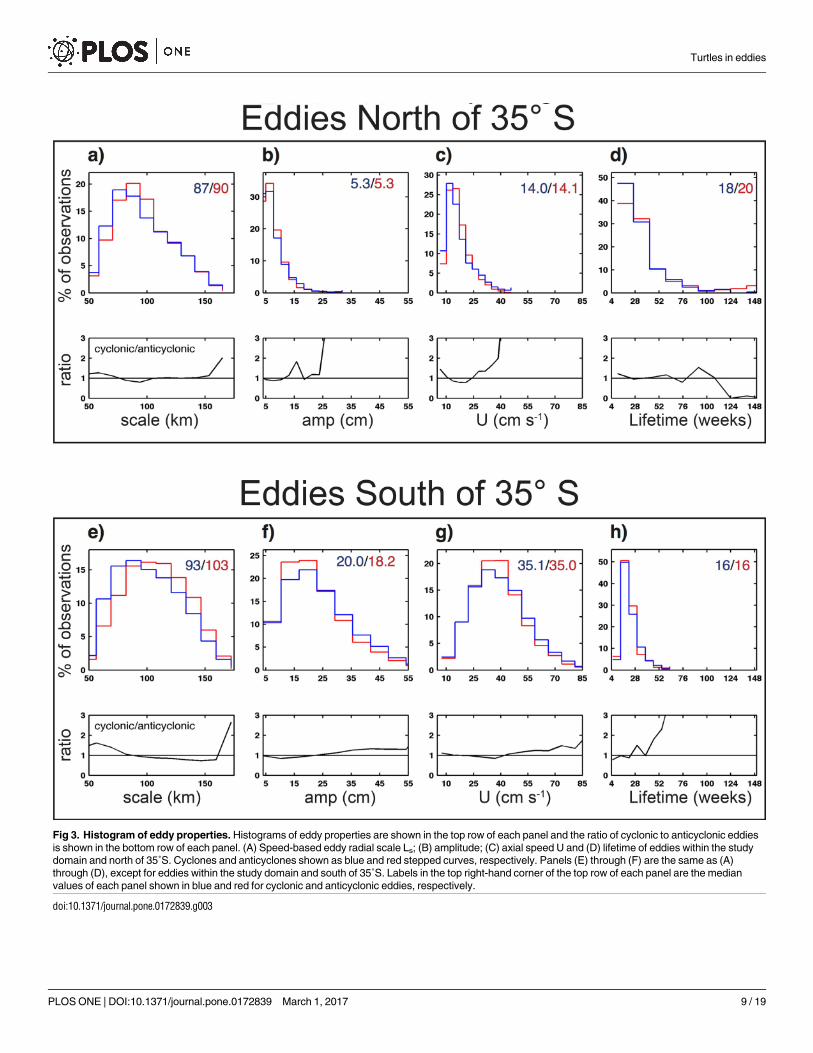
Fig 3. Histogram of eddy properties. Histograms of eddy properties are shown in the top row of each panel and the ratio of cyclonic to anticyclonic eddies

is shown in the bottom row of each panel. (A) Speed-based eddy radial scale Ls; (B) amplitude; (C) axial speed U and (D) lifetime of eddies within the study

domain and north of 35˚S. Cyclones and anticyclones shown as blue and red stepped curves, respectively. Panels (E) through (F) are the same as (A)

through (D), except for eddies within the study domain and south of 35˚S. Labels in the top right-hand corner of the top row of each panel are the median

values of each panel shown in blue and red for cyclonic and anticyclonic eddies, respectively.

doi:10.1371/journal.pone.0172839.g003

Turtles in eddies

PLOS ONE | DOI:10.1371/journal.pone.0172839 March 1, 2017 9 / 19

negative SST’ is located outside of the eddy periphery in the northeast quadrant. Northern

cyclones contain a primary pole of elevated CHL to the north and a region of low CHL to

southeast (Fig 4B). The composite SST’ of these cyclones is characterized by a primary pole of

negative SST’ that extends from the eddy core into the northwest quadrant and a secondary

pole of positive SST’ to the east (Fig 4D). The dipole structure of the composite in the northern

eddies suggests that eddy-induced perturbations of SST and CHL are primarily caused by

advection of ambient gradients around the eddy periphery (“eddy stirring” [37]). It is impor-

tant to note, however, that the anomalies are not zero at the eddy centers, as would be expected

from the influence of eddy stirring alone, suggesting that other mechanisms (i.e. “eddy pump-

ing” [34]) may be important in this region.

In the southern subregion, the observed geographical structure of eddy-induced CHL’’ and

SST’ is best described as a monopole with negative CHL’’ and positive SST’ in the interiors of

anticyclones (Fig 4E and 4G) and positive CHL’’ with negative SST’ within the interiors of

cyclones (Fig 4F and 4H). The exact mechanism generating the observed monopoles of CHL’’

and SST’ in these eddies is ambiguous, as there are at least two processes that could be respon-

sible for the observed patterns. In the case of CHL, Gaube et al. [37] showed that the observed

CHL’’ in these eddies is consistent with trapping of elevated or depressed CHL during forma-

tion of cyclones and anticyclones, respectively. Upwelling and downwelling occurring during

the intensification of cyclones and anticyclones can also generate these same patterns in CHL’’

Fig 4. Eddy-centric composite of CHL and SST. Composite medians of CHL’’ (left two columns) and SST anomalies (right two columns) for eddies in

water depths in excess of 3,000 m. (A,C) Anticyclones and (B,D) cyclones north of 35˚S. (E,G) Anticyclones and (F,H) cyclones south of 35˚S. The x and y

axes if each panel have been scaled by the horizontal speed-based eddy radial scale Ls. The contours overlaid on each composite are the composite median

of SLA at an interval of 3 cm, negative contours shown as dashed curves. Note different colorbar scaling used in the for observations north and south of

35˚S.

doi:10.1371/journal.pone.0172839.g004

Turtles in eddies

PLOS ONE | DOI:10.1371/journal.pone.0172839 March 1, 2017 10 / 19

and SST’ via vertical displacement of the pycnocline and the associated effects on temperature

and nutrient availability.

Observations of juvenile loggerhead sea turtles and surface drifters in

eddies

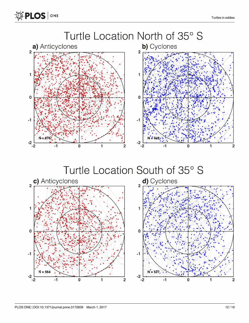
In waters deeper than 3,000 m, turtles were observed to be within eddies (r� 2Ls) 65% of the

time. In the northern subregion, a total of 876 and 948 daily turtle positions were observed

within 2Ls of anticyclones and cyclones, respectively (Fig 5A and 5B). The binning of the daily

positions observations as a function of distance from the eddy centers and normalization by

the area of the annulus defined by each radial bin revealed that turtles were significantly more

likely to be associated with the outer-cores of anticyclones than the outer-cores of cyclones

(Fig 6A). When integrated over the eddy cores (distance r� Ls), the number of daily turtle

locations per unit area was significantly larger in the interiors of anticyclones compared with

cyclones (α = 0.1, not shown). Outside of the eddy core, turtles appeared to be associated more

with the peripheries of cyclones than anticyclones. This raises the question, were turtles modi-

fying their behavior to interact with and remain in these eddy subregions, or is this the result

of the passive advection?

By repeating the above analysis on surface drifters, we were able to address the role of pas-

sive advection in structuring the observed distribution of turtles in different eddy subregions.

It is important to note that drifters are constrained to the surface, whereas turtles are not, an

important caveat noted by other studies [15]. Analysis of the pressure recording tags affixed to

a subset of 5 turtles revealed that when the turtles were below the surface, they attained a maxi-

mum depth between 10 and 100 m 84% of the time (see [16] for a summary of dive depths for

these turtles), suggesting that when diving, turtles often occupy the zone near where the drift-

ers are drogued. Even in light of the differences in drifter configuration and turtle behavior,

the comparison of the passive advection of drifters to the movement of turtles has yielded valu-

able insight into the active movement and foraging behavior of turtles (e.g., [39]).

Histograms of the number of drifters observed as a function of radial distance revealed no

significant difference between the interiors of cyclones and anticyclones (Fig 6B). In the eddy

peripheries, drifters were more likely to occupy anticyclones than cyclones, which was the

opposite of what is observed for turtles (c.f. Fig 6A and 6B). These results suggest that juvenile

loggerhead turtles in the BMC are not passively advected by ocean currents, which is not sur-

prising as previous studies of turtles ranging from the neonatal stage and juveniles have shown

that their trajectories differed substantially from those of passive drifters [24, 40, 41] and the

paths of ambient ocean currents [21].

Another metric analyzed here to investigate if turtles modify their behavior to interact with

or remain in particular regions of eddies is the median turtle swimming speed Vs (Eq 3) when

associated with eddies. Median Vs ranged from ~ 14 cm s-1 to 30 cm s-1 (Fig 6C and 6F), which

is slightly larger than the speeds reported for loggerhead turtle hatchlings [42, 43] and thus

considered to be biologically feasible for juveniles of the same species. Turtles that were ac-

tively feeding, or were choosing to remain within a specific area, were expected to have a

slower Vs than turtles that are seeking suitable foraging habitat. Although there were not sig-

nificant differences in Vs in the inner cores of the two types of eddies, swimming speed was

higher in the outer cores of cyclones (Fig 6C). This behavior may have contributed to the

lower abundance of turtles in the outer cores of cyclones relative to that in anticyclones, given

that the distributions of drifters in those same eddy subregions are equal. Swimming speed

was also significantly elevated along the periphery of anticyclones when compared to cyclones

(Fig 6C; note that the confidence intervals in the inner periphery are just barely distinct from

Turtles in eddies

PLOS ONE | DOI:10.1371/journal.pone.0172839 March 1, 2017 11 / 19

Turtles in eddies

PLOS ONE | DOI:10.1371/journal.pone.0172839 March 1, 2017 12 / 19

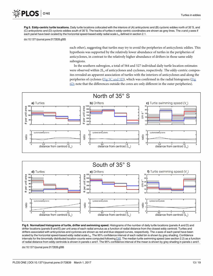
each other), suggesting that turtles may try to avoid the peripheries of anticyclonic eddies. This

hypothesis was supported by the relatively lower abundance of turtles in the peripheries of

anticyclones, in contrast to the relatively higher abundance of drifters in those same eddy

subregions.

In the southern subregion, a total of 564 and 527 individual daily turtle location estimates

were observed within 2Ls of anticyclones and cyclones, respectively. The eddy-centric compos-

ites revealed an apparent association of turtles with the interiors of anticyclones and along the

peripheries of cyclones (Fig 5C and 5D), which was confirmed in the radial histograms (Fig

6D; note that the differences outside the cores are only different in the outer peripheries).

Fig 5. Eddy-centric turtle locations. Daily turtle locations collocated with the interiors of (A) anticyclonic and (B) cyclonic eddies north of 35˚S, and

(C) anticyclonic and (D) cyclonic eddies south of 35˚S. The tracks of turtles in eddy-centric coordinates are shown as grey lines. The x and y axes if

each panel have been scaled by the horizontal speed-based eddy radial scale Ls defined in section 2.1.

doi:10.1371/journal.pone.0172839.g005

Fig 6. Normalized histograms of turtle, drifter and swimming speed. Histograms of the number of daily turtle locations (panels A and D) and

drifter locations (panels B and E) per unit area of each radial annulus as a function of radial distance from the closest eddy centroid. Turtles and

drifters associated with anticyclones and cyclones are shown as red and blue stepped curves, respectively. The x axes of each panel have been

scaled by the horizontal speed-based eddy radial scale Ls. The 95% confidence interval of each radial bin is shown by grey shading. Confidence

intervals for the binomially distributed location counts were computed following [38]. The median turtle swimming speed (see section 2.2) as a function

of radial distance from eddy centroids is shown in panels c and f. The 95% confidence interval of the mean is shown by grey shading in panels c and f.

doi:10.1371/journal.pone.0172839.g006

Turtles in eddies

PLOS ONE | DOI:10.1371/journal.pone.0172839 March 1, 2017 13 / 19

Drifters, on the other hand, were equally likely to be associated with the inner cores of anticy-

clones versus cyclones, and were only 5% more likely to be in the outer-core of anticyclones

than cyclones (Fig 6E). Median Vs was significantly slower in the cores and inner peripheries

of anticyclones, when compared to their outer peripheries (Fig 6F). This suggests that when

turtles were in the cores and inner peripheries of anticyclones, they slowed their swimming,

possibly in an attempt to remain in this eddy subregion. On the other hand, when turtles

found themselves on the outer periphery of anticyclones, they elevated their swimming speed,

possibly to move to a different eddy subregion. It is also interesting to note that median swim-

ming speed was significantly elevated in the cores of cyclones (Fig 6F), which may reflect

avoidance of those features.

A possible bias may have been introduced from the colocation of turtles to eddies with life-

times greater than or equal to 12 weeks. A turtle could have been assigned to a particular long-

lived eddy, when in fact it was closer to an ephemeral eddy, with lifetime shorter than 12

weeks. The analysis presented throughout this section was repeated using an eddy lifetime cut-

off of 4 weeks, which did not yield any significant differences in the results. Therefore, we do

not consider our results to be particularly sensitive to the collocation of turtles with long-lived

eddies instead of ephemeral eddies with lifetimes shorter than 12 weeks.

Possible mechanisms controlling the distribution of turtles in eddies

The most pronounced signal in the eddy-centric distribution of turtles is the apparent prefer-

ence for the interiors of anticyclones in the southern region (Fig 6D), which were associated

with low CHL’’ and warm SST’ (Fig 4E and 4G). We suggest two possible hypotheses for the

association of turtles with the cores of anticyclones south of 35˚S: (1) Turtles were passively

advected south 35˚S in the interiors of anticyclones that propagate south until certain cues

(perhaps temperature or elevated CHL) indicate the need for northward movement on the

part of the turtle. (2) Turtles were actively modifying their behavior to interact with and

remain in anticyclones south of 35˚S possibly because of suitable foraging conditions associ-

ated with low CHL, decreased predation, elevated ambient temperatures which influence turtle

growth rates, feeding behavior, movement speed and physiological and immune competence

[44, 45] or other reasons not discernable from the data analyzed here.

If turtles were passively advected southward inside anticyclones, we expect the proportion

of turtle locations in anticyclones to be higher during southward propagation across the 35˚S

boundary when compared to northward propagation across the boundary. Indeed, turtles are

11% more likely to be in anticyclones while moving southward versus northward. Thus, we

conclude that turtles may be passively advected southward inside anticyclones, however, it is

also possible that turtles modify their behavior to interact with the pelagic ecosystems trapped

within these southern anticyclones.

In the southern subregion, VS was significantly slower in the cores and inner peripheries of

anticyclones, when compared to the outer peripheries (Fig 6F). This leads to the question,

what are the physical and biological characteristics of anticyclones that could cause turtles to

lower their swimming speed? The analysis of eddy-centric CHL and SST anomaly composites

in section 3.2 revealed that south of 35˚S the interiors of anticyclones and periphery of

cyclones are characterized by low CHL and warm SST anomalies.

As turtles do not feed on CHL, they were likely preferentially seeking out some other envi-

ronmental or biological property that is associated with low CHL and warm water observed in

anticyclones in the southern BMC region. Numerous investigations of the stomach contents of

deceased juvenile loggerhead sea turtles (size ranging from 5.2 to 30.0 cm strait carapace

length) report a high concentration of gelatinous organisms contained therein (see review by

Turtles in eddies

PLOS ONE | DOI:10.1371/journal.pone.0172839 March 1, 2017 14 / 19

Bjorndal et al. [46]). Parker at al. [47] found that Janthina sp. (a pelagic gastropod) was the

most common prey item for oceanic stage loggerheads (size ranging from 13.5 to 74.0 cm

curved carapace length) in the North Pacific followed by Carinaria carinaria (a gastropod) and

a colonial hydroid Velella velella. In addition, Bowen et al. [48] found that in the Eastern

Pacific, large aggregations of juvenile loggerhead sea turtles foraged on pelagic red crabs. In

the North Atlantic, investigation of the stomach contents of 12 oceanic-stage loggerhead tur-

tles concluded that the V. velella was the most abundant prey, both in terms of volume and fre-

quency [49].

The particular properties of anticyclones in the southern regions that cue juvenile logger-

head turtles to remain within the eddy cores are not directly discernable from the data ana-

lyzed here. One possible mechanism is that enhanced foraging success in anticyclones, be it

the result of elevated prey or the metabolic advantage associated with warmer water, results in

turtles modifying their behavior to actively remaining in anticyclones.

Comparison to previous investigations of the interaction turtles with

eddies

In an investigation of non-reproductive loggerhead sea turtles in the East China Sea, Kobaya-

shi et al. [10] computed the proximity-probability of turtles to the centers and peripheries of

mesoscale eddies. Using this metric, they concluded that turtles avoided the peripheries of

energetic cyclonic eddies. In the analysis presented here, we normalize the number of turtle

colocations by the area of each radial band (see section 2.6), removing the bias resulting from

the relatively large area encompassed by the eddy periphery compared to the core. Using this

method, we find that turtles in the southern region are significantly more likely to associate

with the interiors of anticyclonic eddies, contrary to what was observed in the East China Sea.

In order to assess the sensitivity of our results to this normalization, we re-analyzed our obser-

vations using the methods of [10] and found the proportion of turtles in proximity to the

peripheries of eddies was greater than eddy centers (not shown). Thus, the results are highly

sensitive to whether or not the relative proportions of turtle populations in the various radial

bands are normalized by area.

The tagging of adult Leatherback turtles (Dermochelys coriacea) has revealed that individu-

als spend considerable time in the interiors of anticyclonic eddies. In the Bay of Biscay in the

Northeastern Atlantic, a single leatherback turtle was observed to circle the center of a large

anticyclonic eddy for 33 days [50]. In the Indian Ocean, two leatherback turtles were observed

to migrate southward from their nesting beaches along the coast of southeastern Africa and

spend multiple days in a series of anticyclonic eddies [51, 52]. In both of these studies the

authors suggested that the anticyclonic eddies were likely regions of elevated foraging success.

Furthermore, the analysis in [37] suggests that anticyclones along the coast of southeastern

Africa have low CHL which is consistent with the results presented here for the BMC south of

35˚S.

Summary and conclusions

By collocating the trajectories of juvenile loggerhead sea turtles with the tracks of mesoscale

eddies, we provided evidence of the preferential use of the interiors of anticyclonic eddies by

juvenile loggerhead turtles in the offshore region of the BMC south of 35˚S. These eddies were

associated with low CHL and warm SST anomalies. We present two possible mechanisms for

the observed affinity of turtles towards anticyclones: (1) turtles were passively advected south

of 35˚S in the interiors of anticyclones, and (2) turtles were actively seeking out water masses

trapped within anticyclones south of 35˚S, possibly because of suitable foraging conditions,

Turtles in eddies

PLOS ONE | DOI:10.1371/journal.pone.0172839 March 1, 2017 15 / 19

decreased predation, elevated SST, or other reasons not discernable from the data analyzed

here. Inferred swimming speeds were lower in the cores and inner peripheries of anticyclones,

and higher in their outer peripheries, which is consistent with a behavioral preference for the

interiors of these features. Swimming speeds were also elevated in the cores of cyclones, which

is suggestive of their avoidance of such features. Further targeted field studies assessing the

interaction of the turtles with their prey are needed to identify the primary mechanisms result-

ing in the observed preference for the cores of anticyclonic eddies.

This study revealed that by combining contemporaneous satellite observations of CHL,

SST, and SLA, with the trajectories of turtles, drifters and eddies, new understanding can be

obtained about association of turtles with mesoscale eddies in the open ocean. This methodol-

ogy can be applied to the investigation of the use of mesoscale eddies by any organism that can

be tracked in space and time with precision sufficient to resolve motions at the oceanic meso-

scale. This knowledge can aid in the identification of critical habitat in the open-ocean, which

could be of use in the protection of endangered or over-harvested species, for example via the

creation of mobile marine protected areas [53].

Supporting information

S1 File. Turtle location data. The turtle location data used in this study. Data are stored in

NetCDF format.

(NC)

Acknowledgments

Thanks to Uruguay’s and Brazil’s scientific observers for deploying satellite transmitters and

providing accompanying information on the bycatch turtles, as well as the skippers and crew

of fishing vessels where turtles were captured and equipped with transmitters. Funding for sat-

ellite transmitters and ARGOS satellite time was made available for this project by NOAA

National Marine Fisheries Service, Pacific Island Fisheries Science Center. We thank Dr. Fran-

cesco d’Ovidio for helpful comments and discussion on an earlier version of the manuscript

and three anonymous reviewers for constructive feedback. We acknowledge Collecte Localis

Satellites, AVISO (http://www.aviso.oceanobs.com) for the SLA observations, NOAA’s Atlantic

Oceanographic and Meteorological Laboratory AOML (http://www.aoml.noaa.gov/phod/index.php) for the drifter observations, NASA MEaSUREs Ocean Color Product Evaluation

Project (ftp://ftp.oceancolor.ucsb.edu) for the CHL observations, NOAA National Climatic

Data Center for the SST observations (data available at ftp://eclipse.ncdc.noaa.gov/pub/OI-

daily-v2/NetCDF), and NOAA National Geophysical Data Center NGDC (http://www.ngdc.noaa.gov/mgg/fliers/06mgg01.html) for the global bathymetric data. A Woods Hole Postdoc-

toral Fellowship awarded to PG and NASA grant NNX13AE47G funded this work. CB is

grateful for support from NOAA and the NSF-GRFP (Grant No. 1314109). DJM gratefully

acknowledges support from NASA and NSF.

Author Contributions

Conceptualization: PG DM CB.

Formal analysis: PG CB.

Resources: CB AD PM BG NM YS.

Supervision: DM.

Turtles in eddies

PLOS ONE | DOI:10.1371/journal.pone.0172839 March 1, 2017 16 / 19

Visualization: PG.

Writing – original draft: PG.

Writing – review & editing: DM YS CB.

References1. Benitez-Nelson CR, Bidigare RR, Dickey TD, Landry MR, Leonard CL, Brown SL, et al. Mesoscale

eddies drive increased silica export in the subtropical Pacific Ocean. Science. 2007; 316(5827):1017–

21. doi: 10.1126/science.1136221 PMID: 17510362

2. Falkowski PG, Ziemann D, Kolber Z, Bienfang PK. Role of eddy pumping in enhancing primary produc-

tion in the ocean. Nature. 1991; 352(6330):55–8.

3. McGillicuddy DJ Jr., Anderson LA, Bates NR, Bibby T, Buesseler KO, Carlson CA, et al. Eddy/wind

interactions stimulate extraordinary mid-ocean plankton blooms. Science. 2007; 316(5827):1021–6.

doi: 10.1126/science.1136256 PMID: 17510363

4. Thompson PA, Pesant S, Waite AM. Contrasting the vertical differences in the phytoplankton biology of

a dipole pair of eddies in the south-eastern Indian Ocean. Deep Sea Research Part II: Topical Studies

in Oceanography. 2007; 54(8–10):1003–28.

5. GodøOR, Samuelsen A, Macaulay GJ, Patel R, Hjøllo SS, Horne J, et al. Mesoscale eddies are oases

for higher trophic marine life. PloS one. 2012; 7(1):e30161. doi: 10.1371/journal.pone.0030161 PMID:

22272294

6. Hobday AJ, Hartog JR. Derived Ocean Features for Dynamic Ocean Management. Oceanography.

2014; 27(4):134–45.

7. Chelton DB, Schlax MG, Samelson RM. Global observations of nonlinear mesoscale eddies. Progress

in Oceanography. 2011; 91(2):167–216.

8. Gaube P, Chelton DB, Samelson RM, O’Neill LW, Schlax MG. Satellite Observations of Mesoscale

Eddy-Induced Ekman Pumping. Journal of Physical Oceanography. 2015; 45:104–32.

9. McGillicuddy DJ Jr. Mechanisms of Physical-Biological-Biogeochemical Interaction at the Oceanic

Mesoscale. Ann Rev Mar Sci. 2016; 8:125–59. doi: 10.1146/annurev-marine-010814-015606 PMID:

26359818

10. Kobayashi DR, Cheng I-J, Parker DM, Polovina JJ, Kamezaki N, Balazs GH. Loggerhead turtle (Caretta

caretta) movement off the coast of Taiwan: characterization of a hotspot in the East China Sea and

investigation of mesoscale eddies. ICES Journal of Marine Science: Journal du Conseil. 2011; 68

(4):707–18.

11. Mansfield KL, Wyneken J, Porter WP, Luo J. First satellite tracks of neonate sea turtles redefine the

‘lost years’ oceanic niche. Proceedings of the Royal Society of London B: Biological Sciences. 2014;

281(1781):20133039.

12. Polovina J, Uchida I, Balazs G, Howell EA, Parker D, Dutton P. The Kuroshio Extension Bifurcation

Region: a pelagic hotspot for juvenile loggerhead sea turtles. Deep Sea Research Part II: Topical Stud-

ies in Oceanography. 2006; 53(3):326–39.

13. Foley AM, Schroeder BA, Hardy R, MacPherson SL, Nicholas M, Coyne MS. Postnesting migratory

behavior of loggerhead sea turtles Caretta caretta from three Florida rookeries. Endangered Species

Research. 2013; 31:129–42.

14. Polovina JJ, Balazs GH, Howell EA, Parker DM, Seki MP, Dutton PH. Forage and migration habitat of

loggerhead (Caretta caretta) and olive ridley (Lepidochelys olivacea) sea turtles in the central North

Pacific Ocean. Fisheries Oceanography. 2004; 13(1):36–51.

15. Fossette S, Putman NF, Lohmann KJ, Marsh R, Hays GC. A biologist’s guide to assessing ocean cur-

rents: a review. Marine Ecology Progress Series. 2012; 457:285–301.

16. Barcelo C, Domingo A, Miller P, Ortega L, Giffoni B, Sales G, et al. High-use areas, seasonal move-

ments and dive patterns of juvenile loggerhead sea turtles in the Southwestern Atlantic Ocean. Marine

Ecology Progress Series. 2013; 479:235–50.

17. Mora O, Domingo A. Informe sobre el Programa de Observadores a bordo de la flota atunera uruguaya

(1998–2004). Collect Vol Sci Pap ICCAT. 2006; 59(2):608–14.

18. Marcovaldi MA, Dei Marcovaldi GG. Marine turtles of Brazil: the history and structure of Projeto

TAMAR-IBAMA. Biological conservation. 1999; 91(1):35–41.

19. Coyne M, Godley B. Satellite Tracking and Analysis Tool(STAT): an integrated system for archiving,

analyzing and mapping animal tracking data. Marine Ecology Progress Series. 2005; 301:1–7.

Turtles in eddies

PLOS ONE | DOI:10.1371/journal.pone.0172839 March 1, 2017 17 / 19

20. James MC, Andrea Ottensmeyer C, Myers RA. Identification of high-use habitat and threats to leather-

back sea turtles in northern waters: new directions for conservation. Ecology letters. 2005; 8(2):195–

201.

21. Mansfield KL, Saba VS, Keinath JA, Musick JA. Satellite tracking reveals a dichotomy in migration strat-

egies among juvenile loggerhead turtles in the Northwest Atlantic. Marine Biology. 2009; 156(12):2555–

70.

22. Solla D, Shane R, Bonduriansky R, Brooks RJ. Eliminating autocorrelation reduces biological relevance

of home range estimates. Journal of Animal Ecology. 1999; 68(2):221–34.

23. Gaspar P, Georges J-Y, Fossette S, Lenoble A, Ferraroli S, Le Maho Y. Marine animal behaviour:

neglecting ocean currents can lead us up the wrong track. Proceedings of the Royal Society of London

B: Biological Sciences. 2006; 273(1602):2697–702.

24. Putman NF, Mansfield KL. Direct evidence of swimming demonstrates active dispersal in the sea turtle

"lost years". Curr Biol. 2015; 25(9):1221–7. doi: 10.1016/j.cub.2015.03.014 PMID: 25866396

25. Lumpkin R, Pazos M. Measuring surface currents with Surface Velocity Program drifters: the instru-

ment, its data, and some recent results. In Lagrangian Analysis and Prediction of Coastal and Ocean

Dynamics. Cambridge University Press; 2007.

26. Hansen DV, Poulain P-M. Quality control and interpolations of WOCE-TOGA drifter data. Journal of

Atmospheric and Oceanic Technology. 1996; 13(4):900–10.

27. Garver SA, Siegel DA. Inherent optical property inverison of ocean color spectra and its biogeochemical

interpertation: I. Time series from the Sargasso Sea. Journal of Geophysical Research: Oceans. 1997;

102:18607–25.

28. Maritorena S, Siegel DA, Peterson R. Optimization of a semianalytical ocean color model for global-

scale applications. Applied Optics. 2002; 41(15):2705–14. PMID: 12027157

29. Siegel D, Maritorena S, Nelson N, Hansell D, Lorenzi-Kayser M. Global distribution and dynamics of col-

ored dissolved and detrital organic materials. Journal of Geophysical Research: Oceans. 2002; 107

(C12):3228.

30. Gaube P, Chelton DB, Strutton PG, Behrenfeld MJ. Satellite Observations of Chlorophyll, Phytoplank-

ton Biomass and Ekman Pumping in Nonlinear Mesoscale Eddies. Journal of Geophysical Research:

Oceans. 2013; 118:1–22. Epub 10/22/2012.

31. Reynolds RW, Smith TM, Liu C, Chelton DB, Casey KS, Schlax MG. Daily high-resolution-blended anal-

yses for sea surface temperature. Journal of Climate. 2007; 20(22):5473–96.

32. Fu L-L. Pathways of eddies in the South Atlantic Ocean revealed from satellite altimeter observations.

Geophysical Research Letters. 2006; 33(14).

33. Matano R, Palma E, Piola A. The influence of the Brazil and Malvinas Currents on the Southwestern

Atlantic Shelf circulation. Ocean Science. 2010; 6(4):983–95.

34. Oliveira LR, Piola AR, Mata MM, Soares ID. Brazil Current surface circulation and energetics observed

from drifting buoys. Journal of Geophysical Research: Oceans. 2009; 114(C10).

35. Palma ED, Matano RP, Piola AR. A numerical study of the Southwestern Atlantic Shelf circulation:

Stratified ocean response to local and offshore forcing. Journal of Geophysical Research: Oceans.

2008; 113(C11).

36. Chelton DB, Gaube P, Schlax MG, Early JJ, Samelson RM. The Influence of Nonlinear Mesoscale

Eddies on Near-Surface Oceanic Chlorophyll. Science. 2011; 334(6054):328–32. doi: 10.1126/science.

1208897 PMID: 21921157

37. Gaube P, McGillicuddy DJ Jr, Chelton DB, Behrenfeld MJ, Strutton PG. Regional Variations in the Influ-

ence of Mesoscale Eddies on Near-Surface Chlorophyll. Journal of Geophysical Research: Oceans.

2014; 119:1–26.

38. Clopper C, Pearson ES. The use of confidence or fiducial limits illustrated in the case of the binomial.

Biometrika. 1934; 26(4):404–13.

39. Putman NF, Mansfield KL. Direct evidence of swimming demonstrates active dispersal in the sea turtle

“Lost Years”. Current Biology. 2015; 25(9):1221–7. doi: 10.1016/j.cub.2015.03.014 PMID: 25866396

40. Mansfield KL, Wyneken J, Porter WP, Luo J. First satellite tracks of neonate sea turtles redefine the

’lost years’ oceanic niche. Proc Biol Sci. 2014; 281(1781):20133039. PubMed Central PMCID:

PMCPMC3953841. doi: 10.1098/rspb.2013.3039 PMID: 24598420

41. Polovina JJ, Kobayashi DR, Parker DM, Seki MP, Balazs GH. Turtles on the edge: movement of logger-

head turtles (Caretta caretta) along oceanic fronts, spanning longline fishing grounds in the central

North Pacific, 1997–1998. Fisheries Oceanography. 2000; 9(1):71–82.

Turtles in eddies

PLOS ONE | DOI:10.1371/journal.pone.0172839 March 1, 2017 18 / 19

42. Salmon M, Wyneken J. Orientation and swimming behavior of hatchling loggerhead turtles Caretta car-

etta L. during their offshore migration. Journal of Experimental Marine Biology and Ecology. 1987; 109

(2):137–53.

43. Wyneken J, Madrak SV, Salmon M, Foote J. Migratory activity by hatchling loggerhead sea turtles (Car-

etta caretta L.): evidence for divergence between nesting groups. Marine biology. 2008; 156(2):171–8.

44. Lutz PL, Musick JA, Wyneken J. The biology of sea turtles: CRC press; 2002.

45. Schmidt-Nielsen K. Animal physiology: adaptation and environment: Cambridge University Press;

1997.

46. Bjorndal KA, Lutz P, Musick J. Foraging ecology and nutrition of sea turtles. The biology of sea turtles.

1997; 1:199–231.

47. Parker DM, Cooke WJ, Balazs GH. Diet of oceanic loggerhead sea turtles (Caretta caretta) in the cen-

tral North Pacific. Fishery Bulletin. 2005; 103(1):142–52.

48. Bowen B, Abreu-Grobois F, Balazs G, Kamezaki N, Limpus C, Ferl R. Trans-Pacific migrations of the

loggerhead turtle (Caretta caretta) demonstrated with mitochondrial DNA markers. Proceedings of the

National Academy of Sciences. 1995; 92(9):3731–4.

49. Frick MG, Williams KL, Bolten AB, Bjorndal KA, Martins HR. Foraging ecology of oceanic-stage logger-

head turtles Caretta caretta. Endang Species Res. 2009; 9:91–7.

50. Doyle TK, Houghton JD, O’Suilleabhain PF, Hobson VJ, Marnell F, Davenport J, et al. Leatherback tur-

tles satellite-tagged in European waters. Endangered Species Research. 2008; 4:23–31.

51. Luschi P, Lutjeharms J, Lambardi P, Mencacci R, Hughes G, Hays G. A review of migratory behaviour

of sea turtles off southeastern Africa: review article. South African Journal of Science. 2006; 102(1 & 2):

p. 51–8.

52. Luschi P, Sale A, Mencacci R, Hughes G, Lutjeharms J, Papi F. Current transport of leatherback sea

turtles (Dermochelys coriacea) in the ocean. Proceedings of the Royal Society of London B: Biological

Sciences. 2003; 270(Suppl 2):S129–S32.

53. Maxwell SM, Hazen EL, Lewison RL, Dunn DC, Bailey H, Bograd SJ, et al. Dynamic ocean manage-

ment: Defining and conceptualizing real-time management of the ocean. Marine Policy. 2015; 58:42–

50.

Turtles in eddies

PLOS ONE | DOI:10.1371/journal.pone.0172839 March 1, 2017 19 / 19