turbulence transport modelling in gas turbine related applications

Turbulence Transport Modellingin Gas Turbine Related Applications

ANDREAS SVENINGSSON

Department of Applied MechanicsCHALMERS UNIVERSITY OF TECHNOLOGYGoteborg, Sweden, 2006

THESIS FOR THE DEGREE OF DOCTOR OF PHILOSOPHY INTHERMO AND FLUID DYNAMICS


ANDREAS SVENINGSSON

Department of Applied Mechanics

CHALMERS UNIVERSITY OF TECHNOLOGY

Goteborg, Sweden, 2006


Andreas SveningssonISBN 91-7291-739-3

c�

Andreas Sveningsson, 2006

Ny serie nr 2421ISSN 0346-718X

Department of Applied MechanicsChalmers University of TechnologyS-412 96 G oteborg, SwedenPhone +46-(0)31-7721400Fax +46-(0)31-180976

This document was typeset using LATEX.

Printed at Chalmers ReproserviceG oteborg, Sweden


Andreas Sveningsson

Division of Fluid DynamicsDepartment of Applied MechanicsChalmers University of Technology

Abstract

Computational fluid dynamics is a cornerstone in gas turbine engine design.It is used to optimize shapes of turbine and compressor airfoils, to predict heattransfer to gas turbine hot parts, to reduce the amount of pollutants that form whenfuel is burnt, to reduce gas turbine noise and so on. There are still, however, areaswhere the computational methods lack in reliability and need further refinement.One is the modelling of turbulence transport effects on mean flow characteristicsand is the main subject of this thesis. The thesis focuses on RANS predictions ofturbulence and heat transfer, where the unknown turbulence transport terms areclosed using turbulence models based on the eddy-viscosity concept.

The potential of using the ��

turbulence model for heat transfer predic-tions in complex flows is illustrated by computing a three-dimensional stator vanepassage flow. It is shown that the �

� ��model is able to predict the effects

of turbulence on the secondary flow field in the stator passage, and, that the sec-ondary flow field is largely what determines the heat transfer to the vane endwalls.The use of the realizability constraint to prevent unphysical growth of turbulencekinetic energy is also thoroughly discussed.

There are however problems with the ��

model as well. It is in principleunable to resolve turbulence anisotropy and furthermore suffers from predictinglaminar to turbulent boundary layer transition too rapidly. It is shown that the for-mer problem can be dealt with by employing the nonlinear eddy-viscosity modelof Pettersson-Reif (2000). This model is tested in the asymmetric diffuser flowand proves to be capable of very accurate Reynolds stress predictions. This studyalso highlights the strong sensitivity of the mean flow to turbulence closure andsuggests that the near wall modelling is of the utmost importance. In an effortto improve the performance of the �

� ��model in transitional flows the ideas

behind the transition modelling approach of Walters & Leylek (2004) are adaptedto the �

� ��model. Also provided is an overview of the existing literature on the

subject of transition modelling.

Keywords: RANS, V2F, realizability, transition, secondary flow, heat transfer

iii

List of Publications

This thesis is based on the work contained in the following papers:

� A. Sveningsson and L. Davidson, 2004, Assessment of Realizability Con-straints in �

� ��Turbulence Models, International Journal of Heat and

Fluid Flow, 25, 785-794

� A. Sveningsson and L. Davidson, 2005, Computations of Flow Field andHeat Transfer in a Stator Vane Passage Using the �

� � �turbulence model,

ASME Journal of Turbomachinery, 127, 627-634

� A. Sveningsson, B. A. Pettersson-Reif and L. Davidson, 2005, Modellingthe Entrance Region in a Plane Asymmetric Diffuser by Elliptic Relaxation,Submitted to International Journal of Heat and Fluid Flow

� A. Sveningsson, 2005, Transition Modelling–A Review

� A. Sveningsson, 2005, Towards an Extension of the ��

Model for Tran-sitional Flows

Division of Work Between Authors

The respondent is the first author of all papers on which this thesis is based, andthe respondent produced all the results.

In the work described in Papers I-II the numerical computations were per-formed with an in-house code, parallelized by Dr. Hakan Nilsson. The respondentimplemented the different versions of the �

� � �model and the coupled TDMA

solver used in these studies. The work of a theoretical nature on the effect ofthe realizability constraint was carried out by the respondent and discussed withProfessor Lars Davidson.

In Paper III most of the modifications to the nonlinear ��

model weresuggested by Anders Pettersson-Reif, who at an early stage believed that the poor

v

modelling performance could be improved by modifying the dissipation rate equa-tion. The respondent carried out most of the analysis of the results, which wasenergetically discussed with the coauthors. All implementations were made bythe respondent.

The work described in Papers IV-V was mainly performed by the respondent.Lars Davidson provided valuable comments throughout the process.

Other Relevant Publications� A. Sveningsson, B. A. Pettersson-Reif and L. Davidson, 2005, Modelling

the Entrance Region in a Plane Asymmetric Diffuser by Elliptic Relaxation,In: Proceedings of the Fourth International Symposium on Turbulence andShear Flow Phenomena, vol 3, 1183-1188, Williamsburg, USA

� A. Sveningsson, 2003, Analysis of the Performance of Different ��

Turbulence Models in a Stator Vane Passage Flow, Licentiate Thesis, Divi-sion of Thermo and Fluid Dynamics, Chalmers University of Technology,Gothenburg

vi

AcknowledgementsThere are several persons without whom this thesis would probably never havebeen written. My supervisor, Professor Lars Davidson, must of course be first inline. Without his encouragement and belief in me as a research student I wouldnot have gotten past the licentiate degree. I am also deeply grateful for all thehours that Lars has spent critically reading my manuscripts, which has certainlyimproved their quality. Thanks also to my co-supervisor, Dr. Hakan Nilsson, forteaching me how to CALC and for helping me with all ICEM pitfalls.

I would also like to express my gratitude to Dr. Anders Petterson-Reif. Thework behind Paper III and the nonlinear model would not have been carried outwithout his devoted support. His appearence at the Department also boosted mymotivation to continue my studies.

I must also mention Docent Gunnar Johansson and Professor Bill George whohave done their best to teach me fractions of what they know about fluid dynamicsin general and turbulence in particular. They have also served as good examplesof fluid dynamics researchers.

Professor Karen Thole, at the Virginia Polytechnic Institute and State Uni-versity, is also gratefully acknowledged for instantly supplying experimental datawhenever needed.

Special thanks also to Dr. Jonas Larsson at Volvo Aero Corporation for all in-struction when I was learning Fluent and for letting me use the computer facilitiesat VAC at the beginning of this project.

The financial and gas turbine technological support of the partners involvedin the Swedish Gas Turbine Center (GTC) is gratefully acknowledged. Specialthanks go to Esa Utriainen for his keen interest in my work and to Sven GunnarSundkvist for the superb management of GTC, from which I learned quite a lot.

Finally, Eva is the oustandingly most important person to this thesis (and notonly the thesis!). Life is easy with You by my side.

A.S.GoteborgJanuary, 2006

vii

Nomenclature

Latin Symbols�true vane chord; turbulence model constant��constant in the realizability constraint�relaxation parameter�turbulent kinetic energy, defined as

�� turbulent length scale�vane pitch��production rate of �� pressure�vane span; source term;

� � � ��mean strain rate tensor,

�� "!$#&% ��'#�"!(�*)+-,Stanton number, defined as .-/10 �32145��67turbulent time scale4mean velocity in 8 -direction45�mean velocity in 8 � -direction� fluctuating velocity in 8 -direction� � fluctuating velocity in 8 � -direction� � � � Reynolds stress tensor9mean velocity in : -direction; secondary velocity; volume;turbulent velocity scale

� fluctuating velocity in : -direction��

turbulence velocity scalar<mean velocity in = -direction> fluctuating velocity in = -direction

ix

Greek Symbols�

boundary layer thickness� � �Kronecker delta� dissipation rate� �� alternating unit tensor� efficiency�eigenvalue of strain rate tensor� dynamic viscosity�� dynamic turbulent viscosity kinematic viscosity� kinematic turbulent viscosity0 density� � turbulent Prandtl number for variable �� fluid propoerty; pressure-strain rate� � vorticity component in 8 � -direction

Subscripts��

inlet�east� external<west> wall

Abbreviations

BFC Boundary Fitted CoordinatesDNS Direct Numerical SimulationGGDH General Gradient Diffusion HypothesisLES Large-Eddy SimulationLKE Laminar Kinetic EnergyRANS Reynolds Averaged Naviers-StokesSMC Second Moment ClosureTDMA Tri-Diagonal Matrix AlgorithTKE Turbulence Kinetic EnergyUDF User-Defined Function

x

Contents

List of Publications v

Acknowledgements vii

Nomenclature ix

1 Introduction 11.1 Motivation . . . . . . . . . . . . . . . . . . . . . . . . . . . . . . 11.2 The Influence of Temperature on Gas Turbine Performance . . . . 41.3 The Need for Endwall Cooling . . . . . . . . . . . . . . . . . . . 71.4 Gas Turbine Secondary Flow Field Structures . . . . . . . . . . . 8

1.4.1 A Secondary Flow Mechanism . . . . . . . . . . . . . . . 81.4.2 The Influence of Secondary Flows on Heat Transfer . . . . 111.4.3 Relevant Past Studies . . . . . . . . . . . . . . . . . . . . 131.4.4 Experimental Test Case for Validation . . . . . . . . . . . 16

1.5 Transition to Turbulence . . . . . . . . . . . . . . . . . . . . . . 171.6 Objectives of the Present Study . . . . . . . . . . . . . . . . . . . 19

2 Turbulence Modelling 212.1 The Closure Problem . . . . . . . . . . . . . . . . . . . . . . . . 212.2 Turbulence Closures . . . . . . . . . . . . . . . . . . . . . . . . 22

2.2.1 Large-Eddy Simulation . . . . . . . . . . . . . . . . . . . 222.2.2 Second Moment Closures . . . . . . . . . . . . . . . . . 232.2.3 The Eddy-Viscosity Concept . . . . . . . . . . . . . . . . 242.2.4 The Standard

� � � Model . . . . . . . . . . . . . . . . . 252.2.5 The �

� � �Model . . . . . . . . . . . . . . . . . . . . . 26

2.2.6 Nonlinear Eddy-Viscosity Models . . . . . . . . . . . . . 292.3 Turbulence Diffusion Models . . . . . . . . . . . . . . . . . . . . 30

2.3.1 The Eddy-Diffusivity Concept . . . . . . . . . . . . . . . 302.3.2 The Generalized Gradient Diffusion Hypothesis . . . . . . 31

xi

2.4 Wall Boundary Conditions for some Turbulent Quantities . . . . . 312.5 Realizability . . . . . . . . . . . . . . . . . . . . . . . . . . . . . 34

2.5.1 Derivation of the Time Scale Constraint . . . . . . . . . . 342.5.2 Alternative Applications of the Constraint . . . . . . . . . 372.5.3 Alternatives to the Realizability Constraint . . . . . . . . 37

3 Numerical Method 413.1 The Solver CALC-BFC . . . . . . . . . . . . . . . . . . . . . . . 413.2 Numerical Domains . . . . . . . . . . . . . . . . . . . . . . . . . 423.3 Boundary Conditions . . . . . . . . . . . . . . . . . . . . . . . . 43

3.3.1 Stator Vane Inlet Boundary Conditions . . . . . . . . . . 443.4 Tri-Diagonal Matrix Algorithms (TDMA) . . . . . . . . . . . . . 45

3.4.1 Segregated TDMA Solver . . . . . . . . . . . . . . . . . 453.4.2 Coupled TDMA Solver . . . . . . . . . . . . . . . . . . . 47

3.5 Notes on the Commercial Software Used . . . . . . . . . . . . . . 49

4 Summary of Papers 514.1 Paper I . . . . . . . . . . . . . . . . . . . . . . . . . . . . . . . . 51

4.1.1 Background . . . . . . . . . . . . . . . . . . . . . . . . . 514.1.2 Discussion of Results . . . . . . . . . . . . . . . . . . . . 52

4.2 Paper II . . . . . . . . . . . . . . . . . . . . . . . . . . . . . . . 524.2.1 Background . . . . . . . . . . . . . . . . . . . . . . . . . 524.2.2 Discussion of Results . . . . . . . . . . . . . . . . . . . . 53

4.3 Paper III . . . . . . . . . . . . . . . . . . . . . . . . . . . . . . . 544.3.1 Background . . . . . . . . . . . . . . . . . . . . . . . . . 544.3.2 Discussion of Results . . . . . . . . . . . . . . . . . . . . 55

4.4 Papers IV and V . . . . . . . . . . . . . . . . . . . . . . . . . . . 564.4.1 Motivation . . . . . . . . . . . . . . . . . . . . . . . . . 564.4.2 Discussion of Results . . . . . . . . . . . . . . . . . . . . 56

5 Concluding Remarks 575.1 Stator Vane Passage Flows . . . . . . . . . . . . . . . . . . . . . 575.2 Separation in the Asymmetric Diffuser . . . . . . . . . . . . . . . 605.3 Transition . . . . . . . . . . . . . . . . . . . . . . . . . . . . . . 605.4 Suggestions for Future Work . . . . . . . . . . . . . . . . . . . . 61

xii

Chapter 1

Introduction

1.1 Motivation

Consider the flow in a breath of air, the mixing of milk in a cup of coffee, the flowbehind any airborne animal or man-made object, the smoke exiting a chimney, theair on the leeward side of a poorly set sail, the water whirls in rills or rivers, oreven the Gulf Stream, the fascinating winds in hurricanes and our ever-changingweather system. They, and the vast majority of all other fluid flows, have one thingin common–they are all of a turbulent nature. Before continuing it is necessary todiscuss what is meant by a flow being turbulent, or perhaps equally important, notturbulent. Trying to explain the differences of a turbulent flow and a nonturbulentflow, hereafter referred to as a laminar flow, in words is useless. Consider insteadthe two pictures in Figure 1.1. The laminar flow in the jet to the left consistsof fluid layers (cylinders) that slide along each other as the jet passes smoothlyby. Initially the laminar jet is completely stable but at some distance downstreamthe jet exit it becomes unstable and begins to form large regular vortices thatentrain surrounding fluid, which enhances the mixing and spreading of the jet.The fluid motion seen in Figure 1.1b is very different from that in the laminarjet. It consists of three-dimensional, irregular motions of fluid elements, usuallyreferred to as eddies, of varying size and intensity. These eddies are characteristicof turbulence.

A most important feature of turbulent flows, as compared with laminar ones, isthat these flows have extremely good mixing properties. Consider for example thecareful pouring of one liquid into another, e.g. milk in coffee. The two fluids willof course be mixed to some extent but the process is fairly slow, especially if theinitial fluid motion ceases and all transport takes place on a molecular level. If thenthe mixture is stirred with a spoon the two fluids will almost instantly mix. This is

1

(a) �� (b) �� Figure 1.1: Two photos illustrating the fundamental difference between laminarand turbulent flows. The (white) jet fluid is exiting in a surrounding at rest.Reprinted with permission from S. Gogineni, C. Shih, and A. Krothapalli, theGallery of Fluid Motion 1993, Paper S6. Copyright 1993, American Institute ofPhysics.

due to the creation of three-dimensional irregular motions on a scale much largerthan the molecular level, i.e. turbulence. The turbulent motions have the potentialto rapidly transport fluid particles over relatively large distances and should becompared with the random process of molecular motions on a far smaller scale.In flows where it is difficult to create turbulence, e.g. if we are to carefully mixtwo buckets of viscous paint, the mixing process will be significantly slower. Wethus understand that if we are interested in a fluid flow’s mixing properties it is ofcrucial importance that the effects of turbulence are included.

This project doesn’t at all deal with paint mixing resulting from turbulence.The question is rather how turbulence mixes a fluid of high temperature with afluid of lower temperature and a fluid of high momentum (velocity) with a fluidof low momentum (velocity). The reader is probably wondering why this shouldbe so difficult. Aren’t there fundamental laws that describe the physics of fluidmotion (and turbulence)? There are, but the problem is that this set of equations,given in their most general form, which is indeed needed to describe turbulence,in highly nonlinear and cannot be solved analytically. Why then, the reader mightthink, can’t we use all the fancy methods of numerical analysis, discretize and

2

solve the governing equations in an approximate manner and make sure that theerrors in the approximation are negligible? This is in fact exactly what an in-creasing part of the turbulence research community is doing and is referred to asDirect Numerical Simulations (DNS). There is however a problem with DNS ofturbulent flows. The problem is that every single eddy of the flow, no matter howsmall, must fit in the numerical grid. Consider again the turbulent jet depicted inFigure 1.1b. A fair requirement on resolution of this flow would be that the verysmallest structures seen in the picture should be covered by, say, three to five gridpoints in all three geometrical dimensions. Johansson & Klingmann (1994) mademeasurements of the smallest scales present in a �� wide air jet ( �� )with an exit velocity of � � � /�� ( � �� ) and found that their sizes were inthe order of

�� , i.e. a size comparable to the thickness of a hair, at about20 jet widths downstream of the exit. If we then assume that we need to storedata at three positions across these structures in a computational domain with a�� cross section that is, say, �� long, we end up with approximately�� computational points. The largest meshes of todaycontain on the order of � �� points and we can thus understand that a fully resolvedDNS of the described jet will not be realistic for a long time1. In the meantime wewill somehow have to model the effect of at least the smaller turbulent motions.This modelling, i.e turbulence modelling, is primarily what this project is about.

Turbulence modelling results in models of turbulence that are approximationsof real physics. Regardless of the accuracy of these models they can, with varyingdegree of difficulties in properly defining the problem, be applied to any turbulentfluid flow. Generally speaking, one may say that the cruder the model approxi-mations the easier the model is to use. It shall therefore come as no surprise thatsome of the most popular turbulence models of today are not very sophisticatedand are being used in applications that they were not first designed for. Surpris-ingly enough, however, these models, in the hands of an experienced user, oftenproduce useful results in a wide variety of complex flows.

One area in which turbulence models of varying complexity are being exten-sively used is the design of gas turbine engines. This field also contains the ap-plications for which the model development presented in this thesis are intended.In turbine parts of gas turbine engines one of the most crucial shortcomings of

1Note that the ratio, � , of the largest turbulent structures, comparable to a chacteristic phys-ical length scale, e.g. the width of the jet, to the smallest turbulent structures depends on theReynolds number, �� !#"�$ , as �&%'�(�*),+.-0/ . Thus, for typical industrial applications, wherethe Reynolds number is often one to two orders in magnitude larger and the geometry is muchmore complex, the requirements on resolution is even worse. Note also that the DNS requirementof time resolution, which is equally severe as the space resolution requirement, has been omittedin the present discussion.

3

turbulence models is their inability to give reliable predictions of the effect of tur-bulence transport of heat (i.e. the mixing of hot and cold fluids). The followingsection highlights the importance to these machines of accurately accounting forheat transfer due to turbulence Of equal importance to the overall efficiency of gasturbine engines are accurate predictions of momentum transport due to turbulence(the mixing of high and low speed fluids). If the effects of momentum traqnsportcannot be accounted for correctly, computations that overpredict it may suggesttoo aggressive designs and lead to great reductions in stage efficiency owing tolarge separated regions. Another consequence would be overpredictions of skinfriction losses, which account for about half the loss in stage efficiency of a com-pressor stage (at its design point).

1.2 The Influence of Temperature on Gas TurbinePerformance

The inventors of gas turbine engines were not very concerned about the efficiencyof their machines. They were happy with the fact that their devices were able totransform the internal energy of a fuel into mechanical power output, and the costof the fuel at that time was probably not an issue. As every car owner of todayknows, that situation has changed quite dramatically. The fuel price is all but lowand even the smallest increase in performance can lead to decisive differenceswhen the gas turbine cost-effectiveness is compared with that of the products ofcompeting manufacturers.

The ever increasing efficiency of gas turbines lies today in the range of 35-40%, which of course is a significant improvement since the early days of gasturbine technology. The prospects of further improvements can be illustrated byanalyzing a real gas turbine using the Brayton cycle, which is the ideal thermody-namic cycle for gas turbines. The efficiency of this cycle, � , is

� � � �� (1.1)

where �� is a constant and��

and� ��

are the high and low pressurelevels in the ideal cycle. We thus see that the only way to increase the efficiencyis to either lower

� ��or raise

�� . As

� ��is coupled to the pressure of the

engine surroundings we must raise��

in order to increase the efficiency ofthe gas turbine. Note that there is no explicit temperature dependence present inthe efficiency expression of the Brayton cycle. Nevertheless the temperature ofthe gas entering the (gas) turbine has increased quite dramatically over the last

4

Figure 1.2: Development of gas turbine inlet temperature illustrating the impactof cooling technology.

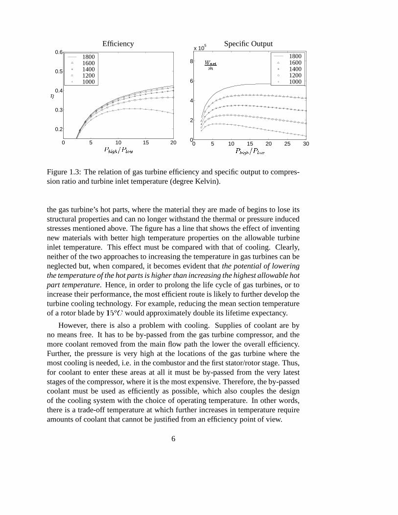
decades as illustrated in Figure 1.2. What then, if not an increase in performance,is the reason for this rise in temperature? In Figure 1.3 the effect of turbine inlettemperature on the performance and specific output (net work output per unitmass flow rate) of a more realistic gas turbine is illustrated. Here a model of asimple cycle gas turbine2 is analyzed and it can be seen that the efficiency, andespecially the specific output, increases with increased inlet temperature. Even ifthe improved efficiency in this cycle is not negligible it is the increase in specificoutput that has been the driving force towards higher temperatures. The benefitfrom an increased specific output is for stationary gas turbines (power plants)simply that a specific engine produces more power as the temperature increasesand for aircrafts that big (heavy) engines may be replaced by smaller ones toincrease the payload. The major problem in further increasing the temperaturesin a gas turbine is that the rise in temperature will increase the heat load on thehot parts of the gas turbine. This increases the thermal stresses in the gas turbinematerial and shortens its lifetime.

An interesting observation can be made in Figure 1.2, which shows the influ-ence of blade cooling on the inlet temperature of the turbine. Without cooling, theturbine’s maximum allowable inlet temperature is restricted by the temperature of

2Isentropic compressor and turbine efficiency of 0.8 and 0.85, respectively.

5

0 5 10 15 20

0.2

0.3

0.4

0.5

0.6

PSfrag replacements

��

�

18001600140012001000

0 5 10 15 20 25 300

2

4

6

8

x 105

PSfrag replacements

��

18001600140012001000

Efficiency Specific Output

��

Figure 1.3: The relation of gas turbine efficiency and specific output to compres-sion ratio and turbine inlet temperature (degree Kelvin).

the gas turbine’s hot parts, where the material they are made of begins to lose itsstructural properties and can no longer withstand the thermal or pressure inducedstresses mentioned above. The figure has a line that shows the effect of inventingnew materials with better high temperature properties on the allowable turbineinlet temperature. This effect must be compared with that of cooling. Clearly,neither of the two approaches to increasing the temperature in gas turbines can beneglected but, when compared, it becomes evident that the potential of loweringthe temperature of the hot parts is higher than increasing the highest allowable hotpart temperature. Hence, in order to prolong the life cycle of gas turbines, or toincrease their performance, the most efficient route is likely to further develop theturbine cooling technology. For example, reducing the mean section temperatureof a rotor blade by �

� �would approximately double its lifetime expectancy.

However, there is also a problem with cooling. Supplies of coolant are byno means free. It has to be by-passed from the gas turbine compressor, and themore coolant removed from the main flow path the lower the overall efficiency.Further, the pressure is very high at the locations of the gas turbine where themost cooling is needed, i.e. in the combustor and the first stator/rotor stage. Thus,for coolant to enter these areas at all it must be by-passed from the very lateststages of the compressor, where it is the most expensive. Therefore, the by-passedcoolant must be used as efficiently as possible, which also couples the designof the cooling system with the choice of operating temperature. In other words,there is a trade-off temperature at which further increases in temperature requireamounts of coolant that cannot be justified from an efficiency point of view.

6

Improving gas turbine cooling is all but a trivial matter and requires a thor-ough understanding of how the complex flow field in the combustor and the firststator/rotor stage develops. For example, the external gas path flow determines theoptimal locations for the injection of coolant. That is, these locations should idellybe chosen such that most of the injected fluid remains close to the parts exposed tothe hottest flow conditions. The thermal load on the turbine is particularly impor-tant as the first stator vanes are hit by an accelerated, very hot and highly turbulentstream of gas causing high heat transfer rates in the stagnation region of the vanes.Another complicating factor is that the conditions around turbine airfoils (i.e. sta-tor vanes or rotor blades) strongly influence the state of the boundary layer. Thatis, even though the free stream downstream of the combustor is highly disturbed,the strong acceleration around the airfoils makes it difficult to tell whether theairfoil boundary layer will be of a laminar, turbulent or transitional nature. Keep-ing the mixing properties of turbulence discussed in the previous section in mindit should come as no surprise that the heat transfer rates in a turbulent boundarylayer can reach levels several hundred percent higher than those in laminar bound-ary layers. Therefore, numerical methods aimed at facilitating the design of thenext generation of gas turbines engines must be able to accurately account for theeffect of turbulent transport on complex free stream flow structures and boundarylayer heat transfer and must thus also be able to determine the state of boundarylayers.

1.3 The Need for Endwall Cooling

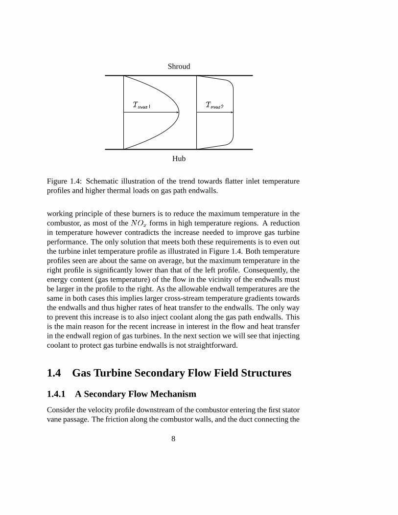
The previous section argued that an efficient way to increase the performance ofgas turbines is to increase the temperature of the gas exiting the combustor. Itwas also shown that this temperature has indeed increased substantially over thelast decades. Further, it was mentioned that the increase in temperature causesthe heat transfer to the turbine airfoil to grow significantly. This is nothing newand, as heat transfer to turbine blades has been studied thoroughly, it is fairlywell understood what is required to keep the temperature of the airfoil surfacessufficiently low. Typically, most of the coolant is injected in the vicinity of theleading edge and remains close to the blade throughout the blade passage as theflow around the blade is, at least when the turbine is operated at design condi-tions, essentially two-dimensional and attached to the blade surface. Recently,however, as energy consumption is continuously growing, increased environmen-tal awareness has led to legislated requirements for reduced levels of pollutantsfrom energy power plants. A consequence of this is the trend of using so calledlow �� ! burners, which substantially reduce the exhaust levels of �� ! . The

7

��

Hub

Shroud

��

Figure 1.4: Schematic illustration of the trend towards flatter inlet temperatureprofiles and higher thermal loads on gas path endwalls.

working principle of these burners is to reduce the maximum temperature in thecombustor, as most of the �� ! forms in high temperature regions. A reductionin temperature however contradicts the increase needed to improve gas turbineperformance. The only solution that meets both these requirements is to even outthe turbine inlet temperature profile as illustrated in Figure 1.4. Both temperatureprofiles seen are about the same on average, but the maximum temperature in theright profile is significantly lower than that of the left profile. Consequently, theenergy content (gas temperature) of the flow in the vicinity of the endwalls mustbe larger in the profile to the right. As the allowable endwall temperatures are thesame in both cases this implies larger cross-stream temperature gradients towardsthe endwalls and thus higher rates of heat transfer to the endwalls. The only wayto prevent this increase is to also inject coolant along the gas path endwalls. Thisis the main reason for the recent increase in interest in the flow and heat transferin the endwall region of gas turbines. In the next section we will see that injectingcoolant to protect gas turbine endwalls is not straightforward.

1.4 Gas Turbine Secondary Flow Field Structures

1.4.1 A Secondary Flow Mechanism

Consider the velocity profile downstream of the combustor entering the first statorvane passage. The friction along the combustor walls, and the duct connecting the

8

Stat

orV

ane

4��

Endwall

Vorticity

� ��(!(�Horseshoe Vortex

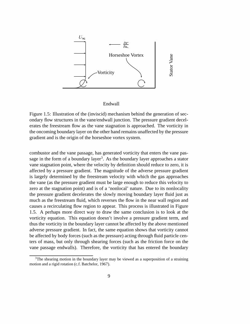
Figure 1.5: Illustration of the (inviscid) mechanism behind the generation of sec-ondary flow structures in the vane/endwall junction. The pressure gradient decel-erates the freestream flow as the vane stagnation is approached. The vorticity inthe oncoming boundary layer on the other hand remains unaffected by the pressuregradient and is the origin of the horseshoe vortex system.

combustor and the vane passage, has generated vorticity that enters the vane pas-sage in the form of a boundary layer3. As the boundary layer approaches a statorvane stagnation point, where the velocity by definition should reduce to zero, it isaffected by a pressure gradient. The magnitude of the adverse pressure gradientis largely determined by the freestream velocity with which the gas approachesthe vane (as the pressure gradient must be large enough to reduce this velocity tozero at the stagnation point) and is of a ‘nonlocal’ nature. Due to its nonlocalitythe pressure gradient decelerates the slowly moving boundary layer fluid just asmuch as the freestream fluid, which reverses the flow in the near wall region andcauses a recirculating flow region to appear. This process is illustrated in Figure1.5. A perhaps more direct way to draw the same conclusion is to look at thevorticity equation. This equation doesn’t involve a pressure gradient term, andthus the vorticity in the boundary layer cannot be affected by the above mentionedadverse pressure gradient. In fact, the same equation shows that vorticity cannotbe affected by body forces (such as the pressure) acting through fluid particle cen-ters of mass, but only through shearing forces (such as the friction force on thevane passage endwalls). Therefore, the vorticity that has entered the boundary

3The shearing motion in the boundary layer may be viewed as a superposition of a strainingmotion and a rigid rotation (c.f. Batchelor, 1967).

9

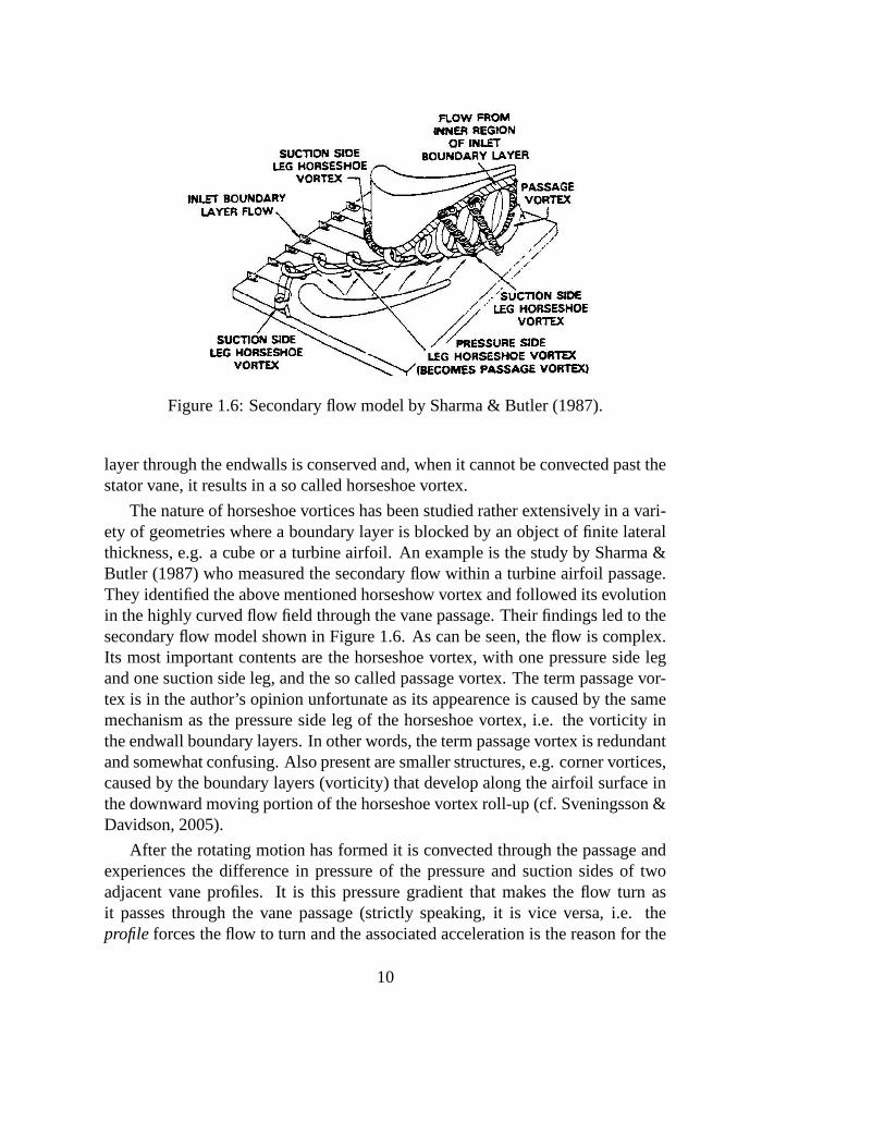
Figure 1.6: Secondary flow model by Sharma & Butler (1987).

layer through the endwalls is conserved and, when it cannot be convected past thestator vane, it results in a so called horseshoe vortex.

The nature of horseshoe vortices has been studied rather extensively in a vari-ety of geometries where a boundary layer is blocked by an object of finite lateralthickness, e.g. a cube or a turbine airfoil. An example is the study by Sharma &Butler (1987) who measured the secondary flow within a turbine airfoil passage.They identified the above mentioned horseshow vortex and followed its evolutionin the highly curved flow field through the vane passage. Their findings led to thesecondary flow model shown in Figure 1.6. As can be seen, the flow is complex.Its most important contents are the horseshoe vortex, with one pressure side legand one suction side leg, and the so called passage vortex. The term passage vor-tex is in the author’s opinion unfortunate as its appearence is caused by the samemechanism as the pressure side leg of the horseshoe vortex, i.e. the vorticity inthe endwall boundary layers. In other words, the term passage vortex is redundantand somewhat confusing. Also present are smaller structures, e.g. corner vortices,caused by the boundary layers (vorticity) that develop along the airfoil surface inthe downward moving portion of the horseshoe vortex roll-up (cf. Sveningsson &Davidson, 2005).

After the rotating motion has formed it is convected through the passage andexperiences the difference in pressure of the pressure and suction sides of twoadjacent vane profiles. It is this pressure gradient that makes the flow turn asit passes through the vane passage (strictly speaking, it is vice versa, i.e. theprofile forces the flow to turn and the associated acceleration is the reason for the

10

pressure difference). The flow turning makes the fluid experience a centripetalforce. This force is greater the higher the velocity of the curved flow. Thus, thefluid close to the endwall, which contains slightly less momentum than fluid inthe freestream, tends to change direction more rapidly than fluid away from thewall. The consequence is that the pressure side leg of the horseshoe vortex movestowards the suction side. This is illustrated in Figure 1.6.

1.4.2 The Influence of Secondary Flows on Heat Transfer

The complex structure of the secondary flow in the gas passage is of great interestin its own right. But let us now return to the problem of cooling the turbineendwalls, or more precisely, endwall cooling under the influence of the secondaryflow depicted above. Consider a boundary layer into which ‘insulating’ coolanthas been injected to protect the endwall from the hot freestream gas, approachinga stator vane. At the location of the horseshoe vortex roll-up, the boundary layer(containing the added coolant) will separate from the endwall surface, which herebecomes exposed to the hot gases of the freestream. That is, downstream of thepoint of separation the efforts spent to cool the endwall surface are more or lesswasted. Recall also the trend of flattening the inlet temperature profiles, whichproduces thin thermal boundary layers. As these layers are thin, only a smallamount of vorticity is needed to bridge the endwall surface at the stagnation pointwith the high temperature freestream fluid.

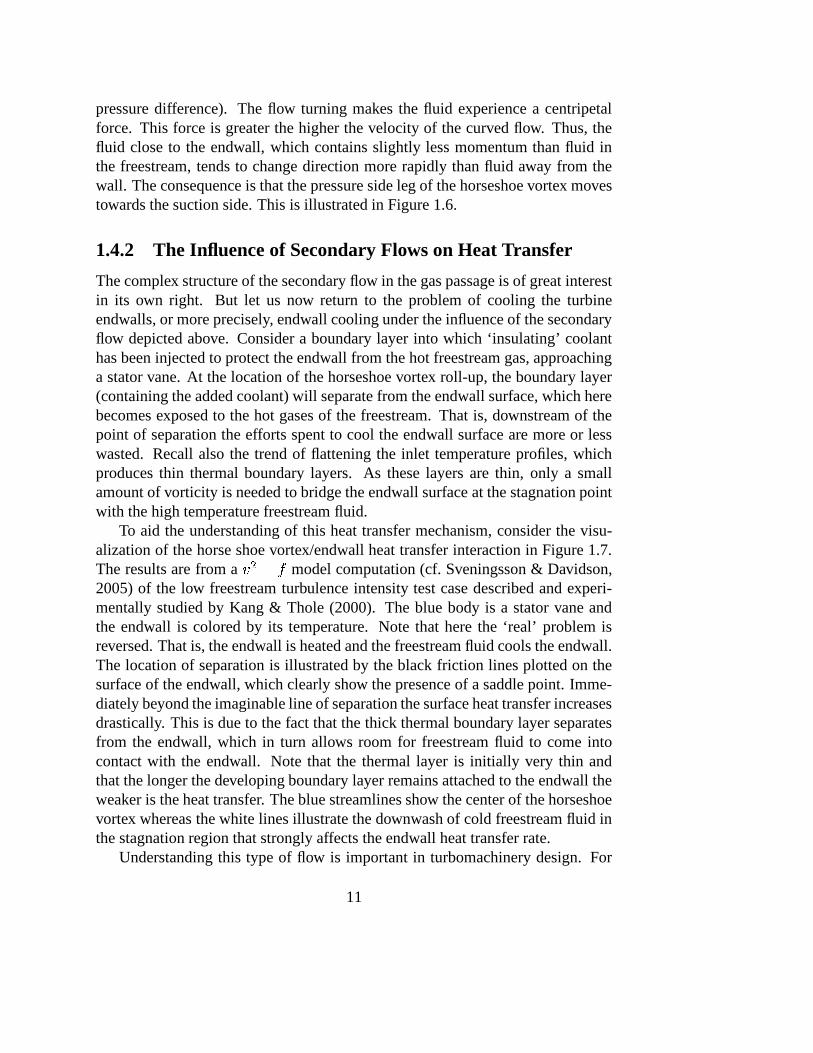
To aid the understanding of this heat transfer mechanism, consider the visu-alization of the horse shoe vortex/endwall heat transfer interaction in Figure 1.7.The results are from a �

� � �model computation (cf. Sveningsson & Davidson,

2005) of the low freestream turbulence intensity test case described and experi-mentally studied by Kang & Thole (2000). The blue body is a stator vane andthe endwall is colored by its temperature. Note that here the ‘real’ problem isreversed. That is, the endwall is heated and the freestream fluid cools the endwall.The location of separation is illustrated by the black friction lines plotted on thesurface of the endwall, which clearly show the presence of a saddle point. Imme-diately beyond the imaginable line of separation the surface heat transfer increasesdrastically. This is due to the fact that the thick thermal boundary layer separatesfrom the endwall, which in turn allows room for freestream fluid to come intocontact with the endwall. Note that the thermal layer is initially very thin andthat the longer the developing boundary layer remains attached to the endwall theweaker is the heat transfer. The blue streamlines show the center of the horseshoevortex whereas the white lines illustrate the downwash of cold freestream fluid inthe stagnation region that strongly affects the endwall heat transfer rate.

Understanding this type of flow is important in turbomachinery design. For

11

Figure 1.7: Visualization of the endwall heat transfer enhancement caused by thepresence of secondary flow structures. The blue body is a stator vane. The con-stant heat flux endwall is colored by its temperature (red is cold, blue is hot). Theblue and white streamlines show the center of the horseshoe vortex pressure sideleg and the downwash of cold freestream fluid that cools the endwall, respectively.The black wall friction lines illustrate the sadde point being formed as a result ofthe horseshoe vortex roll-up.

12

example, any attempt to design an effective cooling of the endwall must take intoaccount the fact that the vortices will lift an ejected insulating cool air film awayfrom the endwall material it is supposed to protect. In such a case the only effectthe coolant will have is to lower the average temperature of the vane passage fluid,i.e. to decrease the efficiency of the turbine. To help our understanding it is highlydesirable to have accurate computational methods that conveniently allow para-metric studies of the influence of geometry, blade loading, freestream turbulence,different cooling concepts, blade counting, inlet flow boundary conditions and soon. The alternative is to perform each such investigation experimentally, whichis expensive. Unfortunately, computations resolving all the flow scales that arepresent are still beyond our scope and we are back at the problem raised in thefirst section–how can we model the influence of turbulent fluctuations?

1.4.3 Relevant Past Studies

For the last fifty years an enormous amount of research has been invested in thearea of gas turbine technology. As discussed in the previous chapter the drivingforce has been requirements for high efficiency and low emissions. The literatureon the subject is vast. The main reason is of course that the subject is very difficult,as almost all the features that make the life of a fluid mechanist hard are present.Some examples are heat transfer itself (which is very difficult both to measure andcompute), three-dimensional flow fields, unsteady interactions between stator andblade rows, high temperatures and pressures, transition, strong compressibilityeffects, high freestream turbulence intensities, streamline curvature, the need foraddition of cooling and so on.

In the world of gas turbine research (as in most other worlds) the standard ap-proach is to try to separate as many of these effects as possible from each otherand study them individually. One disadvantage is that, when dealing with fluidflows, it is difficult to tell what effects can be investigated individually. An exam-ple from this project could be whether is it relevant or not to draw any conclusionsfrom a CFD analysis on how the secondary flow field distributes film cooling air ifthe film cooling itself is not included in the analysis. Another problem is that theresearch area gets split up in many subareas, which makes it difficult to give anoverview of the present research status. Nevertheless, a few studies that highlightthe effect of secondary flows on heat transfer are given below. As the heat trans-fer to endwalls and its dependence on secondary flow structures are of particularinterest in this project, the focus is on studies that include both the flow adjacentto turbine endwalls and the heat transfer to the same.

13

Measurements and Predictions of Gas Turbine Heat Transfer and Flow Field

Much of today’s understanding of the turbine gas path flow field and heat transferstem from experiments carefully conducted during the later decades of the 20thcentury. These experiments not only provide the basic understanding of the un-derlying flow physics but also form a growing data set that can be used to validatethe performance of numerical predictions.

The earliest review of the subject is the paper by Sieverding (1985) that sum-marizes the status of experimental secondary flow research of the time. Of spe-cial interest is the discussion of the development of endwall flow models and thephysics behind the horseshoe vortex system. One of the conclusions is that theproperties of the complex set of vortices depend on the stator vane geometry andthat the leading edge effects are closely related to the incidence angle, which sug-gests variations in the secondary flow field at off design conditions.

Eight years later Simoneau & Simon (1993) made a review of the state of theart in three related areas: configuration specific experiments, fundamental physicsand model development, and code development. All these areas are claimed to beneeded to develop accurate predictive tools for heat transfer in turbine gas paths.A contribution believed to be among the most important is the rotating rig researchby Dunn and coworkers at Calspan, e.g. Dunn (1990), Dunn et al. (1984). Thereasons are that their work includes high time resolution heat flux measurementsobtained using a transient thin film heat flux guage and that theie experimentswere very close to the real world conditions.

Of greater interest to this work is their review of cascade experiments, ofwhich the more important is the work of Langston et al. (1977) and Grazianiet al. (1980), which provides a database suited for code validation. A more recentdatabase covering a range of Reynolds numbers was compiled by Boyle & Russell(1990). Simoneau & Simon (1993) also state that the role of the detailed but lessrealistic cascade experiments is to validate codes and physical models. They alsoincluded a complete list of cascade experiments conducted before 1993.

In the study by Boyle & Russell (1990) local Stanton numbers are determinedfor Reynolds numbers based on inlet velocity and axial chord between 73,000and 495,000 using a uniform heat flux foil and the liquid crystal technique fortemperature measurements. Among their conclusions are that the Stanton numberpatterns are almost independent of both inlet Reynolds number and, which is moresurprising, changes in the inlet boundary thickness and that the secondary flow isstronger for the low Reynolds number cases.

Giel et al. (1998) measured endwall heat transfer in a rotor cascade using thesame method as Boyle & Russell (1990). Measurements are obtained for differ-ent Mach and Reynolds numbers with and without turbulence grid. Eight differ-

14

ent flow conditions were investigated. The endwall heat transfer data presentedhere, along with the aerodynamic data presented by Giel et al. (1996), comprise acomplete set of data suitable for CFD code and model validation. Electronic tab-ulations of all data presented in this paper are available upon request. The sameresearch group also measured the blade heat transfer of the same geometry. Theresults are given in Giel et al. (1999). Kalitzin (1999) computed the heat transferfor this experiment using the �

� ��and Spalart-Allmaras one-equation turbu-

lence models. It was found that the predictions of the Stanton number show mostof the features observed in the experiments but fail to quantitatively predict theheat transfer to the endwall. Similar observations have been made by the turbinecooling group at Siemens, Finspang (Rubensd orffer, private communication).

Another experimental/numerical contribution is the work by Jones and co-workers at the University of Oxford. Their annular cascade facility enables short-duration steady flow to be generated at engine-like conditions for up to one sec-ond. Spencer & Jones (1996) found that the secondary flow field had a greaterinfluence on the casing endwall heat transfer than the hub endwall heat transfer.This was explained by the fact that the hub vortex had lifted from the endwallcloser to the leading edge than the casing endwall vortex. Harvey et al. (1999)found, quite in contradiction to other studies, that the heat transfer rate is stronglyinfluenced by the Reynolds number, an effect that was reproduced in calculations.They also found that the main difference between measurements and calculationsis that the secondary flow effects on the endwall are underestimated.

In the late 1990s a series of experimental and numerical studies by Thole andcoworkes was conducted at the Virginia Polytechnic Institute and State Univer-sity. They investigated the influence of the freestream turbulence level and inletconditions on the flow field and heat transfer in a large scale stator vane passage attwo Reynolds numbers. One finding was that the vane heat transfer is largely de-termined by the level of freestream turbulence, showing augmentations of 80% onthe pressure side, whereas the heat transfer to the endwall depende to a greater ex-tent on the intensity of the secondary flow field. Further, in Hermanson & Thole(2000a) and Hermanson & Thole (2000b), the influence of inlet conditions andMach number effects on the secondary flow is illustrated on the basis of numeri-cal investigations. As detailed measurements of both flow field and heat transferwere available this set of experiment was chosen as test case for the numericalstudy in this project and will be described in Section 1.4.4.

For a more detailed review of gas turbine endwall research, including bothnumerical and experimental investigations, see Rubensd orffer (2002).

15

�

� ��

� � ��

��

�

PSfrag replacements

Splitter plate

Mainflow

Trip wire

Active turbulencegenerator gridb=1.27cm

17.8b

Inlet

16b

measurementlocation

Boundarylayerbleed

Window

Y

XZ

Plexiglass

wall

Shaded area shows thelayout of the heater

Flow removal

17.8b

88b1.9C

4.6C

0.33C

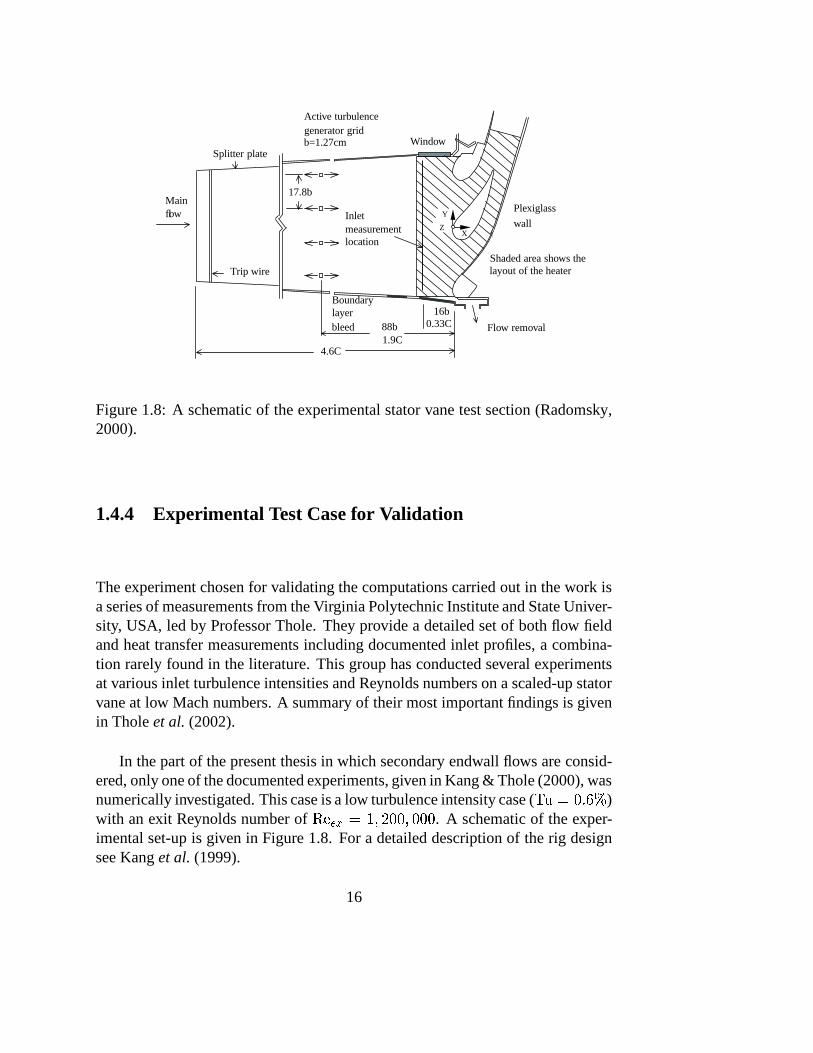
Figure 1.8: A schematic of the experimental stator vane test section (Radomsky,2000).

1.4.4 Experimental Test Case for Validation

The experiment chosen for validating the computations carried out in the work isa series of measurements from the Virginia Polytechnic Institute and State Univer-sity, USA, led by Professor Thole. They provide a detailed set of both flow fieldand heat transfer measurements including documented inlet profiles, a combina-tion rarely found in the literature. This group has conducted several experimentsat various inlet turbulence intensities and Reynolds numbers on a scaled-up statorvane at low Mach numbers. A summary of their most important findings is givenin Thole et al. (2002).

In the part of the present thesis in which secondary endwall flows are consid-ered, only one of the documented experiments, given in Kang & Thole (2000), wasnumerically investigated. This case is a low turbulence intensity case (

�� )

with an exit Reynolds number of �� ! � � � �� . A schematic of the exper-imental set-up is given in Figure 1.8. For a detailed description of the rig designsee Kang et al. (1999).

16

1.5 Transition to Turbulence

Turbulence modelling has for several decades been subject to intense research andhas reached some level of maturity. Today turbulence models exist that are ableto provide accurate predictions of turbulence effects on the mean flow character-istics, given that the mean flow itself is not too complicated. In flows where morecomplex flow features are present, turbulence models still lack in reliability andrequire a more careful (critical) analysis of computed data, at least until new, evenmore powerful methods are developed.

There is however one phenomenon that can cause the most advanced turbu-lence model to fail in flows that are seemingly the most straightforward to com-pute, e.g. the flow over a flat plate. This phenomenon is the transition of a lam-inar flow into a turbulent state and has been studied extensively since OsbourneReynolds, in 1883, was able to relate the parameter 0 9�� / � to the change in flowbehavior as the flow makes a transition to turbulence. The reason for the great in-terest in transition is not only that it plays an important role in many engineeringapplications but also that it raises a more fundamental question about the natureof flow physics and is an example of the problem of determinism and chaos. Itwas only recently, with the aid of Direct Numerical Simulations, that all details ofthe mechanisms behind transition began to become clearer.

A particular field in which there has recently been increased interest in tran-sition physics and its modelling is turbomachinery design. In gas turbines, forexample, transitional phenomena are crucialto the design of the compressor andthe turbines. In the former, about half the loss of stage efficiency at the designpoint owes to skin friction, which is several times larger in a turbulent boundarylayer than in its laminar counterpart. When the compressor is run at off designconditions, however, losses commonly rise rather dramatically as an effect of flowseparation. The extent of the separated regions is largely influenced by the stateof the flow in the separated shear layer. If the separation bubble–which is usuallylaminar at the point of separation–transitions, it will likely reattach to the bladesurface and the loss in efficiency will be limited. Under some circumstances, thetransitional process is slow and the flow reattachment point may move far down-stream on the suction surface and, here, the large separated region causes severelosses in stage efficiency. It thus becomes evident that there is a trade-off betweenthe increase in skin friction losses at design and the risk of massive separation atoff design. The compressor designer must also be aware of the complex interplaybetween separation and transition at off design conditions. These arguments alsoapply to the turbine of the gas turbine engine. Here the situation is further com-plicated by the high temperature environment, and boundary layer transition (toturbulence) dramatically increases the heat load on the turbine airfoils.

17

−0.5 0 0.5 10

5

10

15

PSfrag replacements

�� - � , �� - � , ��Exp. �� Exp. ��

��! #"%$

&('*)#+-,

&('.)0/-,&.'.)21�,

35456

798

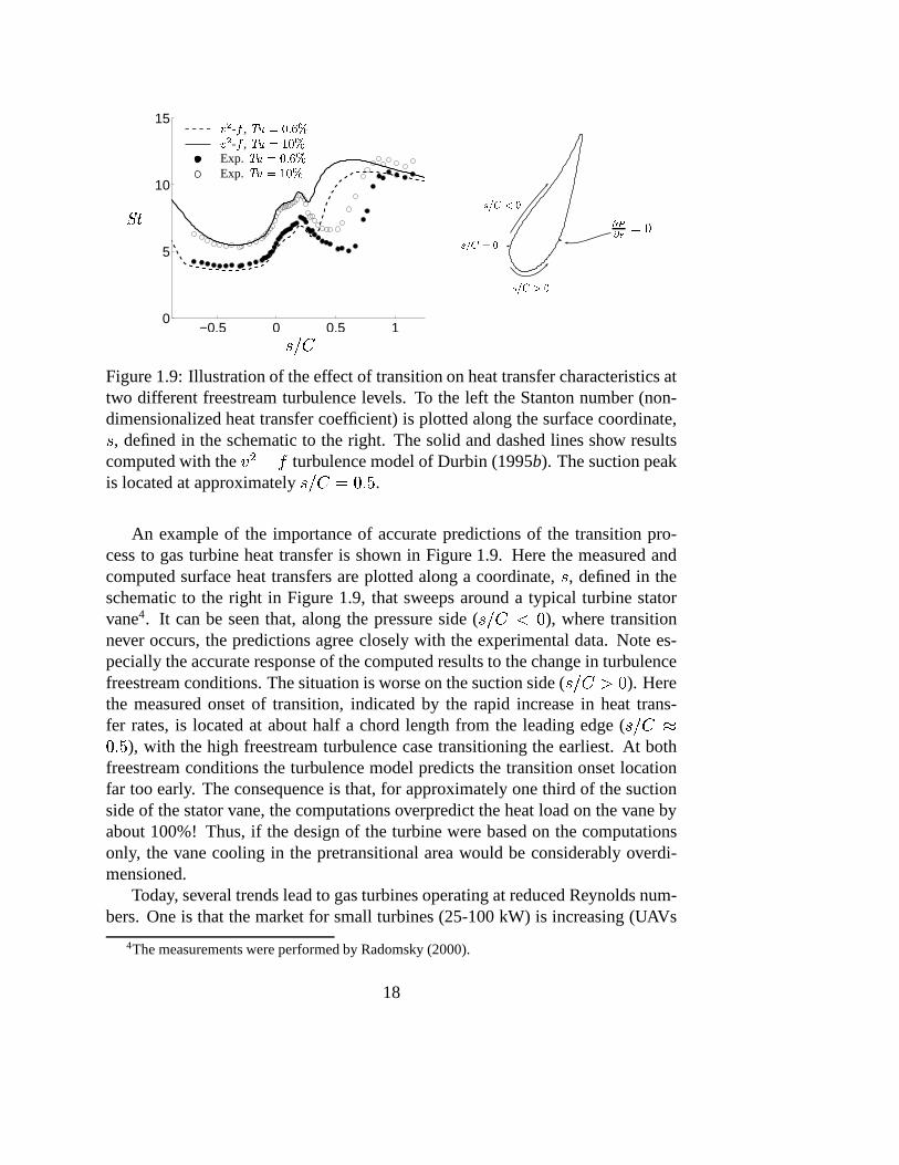
Figure 1.9: Illustration of the effect of transition on heat transfer characteristics attwo different freestream turbulence levels. To the left the Stanton number (non-dimensionalized heat transfer coefficient) is plotted along the surface coordinate,3 , defined in the schematic to the right. The solid and dashed lines show resultscomputed with the :<;0=?> turbulence model of Durbin (1995b). The suction peakis located at approximately 3@4A6CBEDGFIH .

An example of the importance of accurate predictions of the transition pro-cess to gas turbine heat transfer is shown in Figure 1.9. Here the measured andcomputed surface heat transfers are plotted along a coordinate, 3 , defined in theschematic to the right in Figure 1.9, that sweeps around a typical turbine statorvane4. It can be seen that, along the pressure side ( 3@4A6KJLD ), where transitionnever occurs, the predictions agree closely with the experimental data. Note es-pecially the accurate response of the computed results to the change in turbulencefreestream conditions. The situation is worse on the suction side ( 3@4A6NMOD ). Herethe measured onset of transition, indicated by the rapid increase in heat trans-fer rates, is located at about half a chord length from the leading edge ( 3@4A6QPDGFIH ), with the high freestream turbulence case transitioning the earliest. At bothfreestream conditions the turbulence model predicts the transition onset locationfar too early. The consequence is that, for approximately one third of the suctionside of the stator vane, the computations overpredict the heat load on the vane byabout 100%! Thus, if the design of the turbine were based on the computationsonly, the vane cooling in the pretransitional area would be considerably overdi-mensioned.

Today, several trends lead to gas turbines operating at reduced Reynolds num-bers. One is that the market for small turbines (25-100 kW) is increasing (UAVs

4The measurements were performed by Radomsky (2000).

18

powered by gas turbines, intracity Internet links, military vehicles). Another isthe trend towords higher by-pass ratio engines with reduced noise levels. LowerReynolds numbers lead to boundary layers that are less likely to transition to aturbulent state and, when they do, the process is usually slower and the lengthof the transitional part of the boundary layers along the blade surfaces increases.Consequently, the need for accurate predictions of transitional boundary layersalso increases.

1.6 Objectives of the Present Study

Let us conclude this introductory chapter by defining the main objectives of thework presented in this thesis. The overall aim has been to evaluate a specifictype of turbulence modelling, the elliptic relaxation approach suggested by Durbin(1991), in a complex stator vane flow against a suitable set of experimental data,which was to be chosen from the existing literature. As reliable (turbulent) heatflux predictions are of particular interest a requirement for the experimental dataset was that local endwall heat transfer data were documented. Such heat transferdata, together with well documented flow field measurements (including turbu-lence quantities), enable a validation of the chosen turbulence closure’s ability topredict turbulence effects on i) the complex three-dimensional mean flow field ina turbine airfoil passage and ii) airfoil passage heat transfer in general and endwallheat transfer in particular.

A second objective of equal importance has been to investigate how importantthe effects of turbulence really are. For example, are the secondary flow structuressignificantly influenced by the choice of turbulence closure or are the inviscidterms so great that this choice becomes irrelevant? Another question is whetherthe increased heat transfer rates resulting from elevated levels of freestream tur-bulence affect the heat transfer to the endwalls or whether a correct representationof the secondary flow features, which was earlier argued to expose the endwallsto hot freestream fluid, is sufficient?

At the startof this work a relatively new turbulence model began to grow inpopularity. The model, i.e. the �

��model suggested by Durbin (1991), was

claimed to work reasonably well in complex flows involving, for example, flowseparation and seemed also to produce promising results in terms of heat transferpredictions. There was thus great interest on the part of the partners involved inthis project, who were generally rather disappointed with the reliability of turbu-lence heat flux modelling, in investigating this model’s capabilities in the statorflow introduced above and comparing its performance with that of other turbu-lence models in everyday use in industry. Thus a more specific task has been to

19

benchmark the ��

model in gas turbine applications.Even though the �

� � �model has showed promising results, it is, in principle,

unable to account for turbulence anisotropy. This is a problem, as turbulence heattransfer is known to depend rather strongly on the level of anisotropy. It wastherefore decided to investigate the performance of the nonlinear extension to the��

model suggested by Pettersson-Reif (2000). As the model is still underdevelopment it was used only to compute an asymmetric diffuser test case. Theaim of this study was to compare the performance of the nonlinear model withthe original linear version and investigate whether the added model complexityis worthwhile. Note that the linear model does rather well in this flow, which isknown to be extremely sensitive to the turbulence closure, and gets both the largeseparated region and the friction coefficient (which is related to heat transfer)about right. A second objective was therefore to bring clarity to the reason whythe linear �

� ��model produces such good results in this flow and to identify

the underlying mechanisms responsible for the strong sensitivity to turbulenceclosure.

The final, but perhaps most important, subject dealt with in this thesis, at leastif heat transfer is considered, is the problem of determining the state of boundarylayers. Consider for example the perfect turbulence model that always producesexcellent agreement with experimental data in turbulent flows. If this model can-not reliably predict a boundary layer transition from laminar to turbulent (or viceversa) it will not be very useful in predicting5 gas turbine boundary layer flows.Further, the �

� � �model, as almost every other turbulence model, is known to

predict transition too early. Therefore, in an effort to increase the ��

model’sreliability as a gas turbine design tool, the final aim of the work here was to iden-tify a measure to improve its performance in transitional flows. As many attemptshave been made in the past to improve transition modelling it was decided to beginthis modelling effort by making a review of the subject. Thereafter, an approachamong the ones found suitable in the literature survey was to be adopted to the��

model. The aim is then that the resulting turbulence model has the prop-erties of the �

� ��model in turbulent flows and the ability to predict the most

important phenomena in transitional regions.

5There is of course always a possibility to prescribe the location of transition by suppress-ing turbulence in regions where it is known from experience that the boundary layer is likely belaminar. Indeed, this is today a commonly used procedure for dealing with transitional flows.

20

Chapter 2

Turbulence Modelling

2.1 The Closure Problem

As written in the introduction, it is not yet possible to resolve instantaneous tur-bulent fluctuations in flows of industrial importance. However, the industry todayuses numerical simulations of extremely complex fully turbulent flows as an ev-eryday design tool. How is this possible? The answer is that the turbulence itselfis of secondary interest in most applications; only its effect on the mean flowcharacteristics, such as for example the overall drag of a car, is important. This al-lows for computations where the turbulent fluctuations can be accounted for usingstatistical measures of turbulence.

The mean flow equations are obtained by averaging the Navier-Stokes equa-tion. The resulting equations, the so called Reynolds Averaged Navier-Stokesequations, read�� 45�� % 4 � � 45�� 8 �� 0

� �� 8 � % � � 45�� 8 ��

�� 8 �� 4 �� 8 � � �(2.1)

During this procedure all the effects the turbulent fluid motions have on theaveraged flow field are averaged and represented by the additional term � � � � � ,termed the Reynolds stress1.

In the process of averaging we got around the problem of resolving the tinyscales of turbulent motions, which substantially reduces the cost of computingturbulent flows. The great reduction in complexity was not free, however, as

1It should be emphasized here that no modelling has yet been done and that Eqn 2.1 are exact.

21

it generated the unknown Reynolds stress term. This term, which is actually asymmetric tensor with no less than six unknown components, must somehow berelated to other known variables in order to obtain a closed system of equations.This modelling requirement is usually referred to as the turbulence closure prob-lem and some of the suggested closures, in particular the so called eddy-viscositybased closures, will be discussed in the following section.

2.2 Turbulence Closures

The concept of eddy-viscosity modelling is the turbulence modelling approachadopted in this study. Before going into its details, however, two alternative meth-ods to model turbulence will be very briefly discussed for completeness. Theseare Large-Eddy Simulations (LES) and Second Moment Closures (SMC) of whichthe former usually has a clear coupling to eddy-viscosity modelling.

2.2.1 Large-Eddy Simulation

Consider again the discussion given in the introduction on mixing due to turbu-lence. There it was argued that the mixing property of turbulent flows is superiorto that of laminar flows owing to the presence of motions on a much larger scalethan the scale of the molecular motions. The idea behind LES is not that differ-ent. The main concept is that most of the turbulent transport characteristics aregiven by the larger turbulent structures of a flow. The evolution of these ‘large’structures is computed using dynamic equations that are almost identical to theNavier-Stokes equations, i.e. they are described with only a minimal amount ofturbulence modelling. The difference between this approach and DNS is that thesmaller turbulence scales are not resolved and thus require modelling. The eddy-viscosity modelling approach is often adopted for this purpose. As the largerstructures in many fluid flows are indeed the ones that chiefly affect the overallflow picture, the modelling of the smaller scales is only of secondary importance.LES may thus be considered an alternative to DNS in which the computationalfacilities set the bound on the smallest affordable resolved flow structures.

Unfortunately, the dynamic behavior of some flows cannot be characterizedby ‘large’ scale motions alone. The most important examples are flows in whichthe boundary layer development plays a significant role, which includes all ap-plications in which predictions of heat transfer are important. The problem withboundary layers is that the important scales are not significantly larger than thesmallest scales of the flow. Thus, for an LES approach to work properly in a

22

boundary layer, i.e. to fulfill the requirement of resolving its dynamically impor-tant scales, the resolution needs to approach that of a DNS.

A second problem with LES as a numerical tool is its inherent dependence onmesh resolution. Usually, the size of the smallest scales resolved is coupled to theresolution of the numerical grid, i.e. the finer the grid the finer the resolution willbe and, thus, grid dependence becomes an issue. In theory this is not a problem.The mesh size can simply be decoupled from the size of the smallest resolvedscales and the same flow can be computed on a finer grid. The problem is thatthere is a tempting alternative: that is, to use the additional grid points to reducethe need for modelling, i.e. to approach DNS.

2.2.2 Second Moment Closures

Second moment closures constitute the most advanced statistical single point2 tur-bulence closure approach. The modelling basis is the derivation of transport equa-tions for the six individual components of the Reynolds stress tensor by taking the‘second moment’ of the RANS equations (Eqn 2.1). The procedure involves ad-ditional averaging, which results in a large number of additional unknown termsthat require modelling. The conditions for this approach to be more successfulthan directly relating the Reynolds stresses to mean flow quantities are that thenew unknowns are either easy to model or are of subordinate dynamic importanceand that the explicit accessibility of the Reynolds stress components significantlyfacilitates the modelling of turbulence at a reasonable additional computationalexpense.

The strength of this approach is that the Reynolds stresses no longer have to berelated to local flow quantities but are governed by their own transport equations,which allows for nonlocal, or ‘history’, effects. The drawbacks are i) the largenumber of unknown source terms in these transport equations, ii) the fact thatseven transport equations must be solved for the closure of the Reynolds stresses(six equations for the stresses and one to determine a turbulence length scale,usually an equation for the rate of dissipation), iii) that the resulting source termsin the mean momentum equations become large, which has a destabilizing effecton the numerical solution procedure and iv) that the near wall treatment (withimplications for heat transfer predictions) is often problematic.

2The term ‘single point’ refers to the closure of unknown terms using only local mean flow orturbulence quantities.

23

2.2.3 The Eddy-Viscosity Concept

The impact of both large-eddy simulations and second moment closures in indus-try is relatively limited. The reasons are likely that LES is still regarded as beingtoo expensive for everyday industrial use and that SMCs are a bit unreliable interms of numerical stability. Another reason might be a reluctance to abandonwell established procedures, with deficiences the experienced CFD is well awareof, for new, more complex methods with a different set of potential pitfalls. There-fore, the absolutely most commonly used turbulence closures are those based onthe eddy-viscosity concept3. The term is somewhat confusing, however, as it in-fers that the nature of modelled Reynolds stress effects should be similar to thenature of molecular motion, i.e. that Reynolds stress effects are of a diffusive char-acter. This is not at all the case, as the Reynolds stresses stem from the average ofthe nonlinear convective terms in the Navier-Stokes equations.

In a turbulent flow we know from the exact transport equations for the Rey-nolds stresses, � � � � �� , that the generation of Reynolds stresses is proportional tothe mean rate of strain. If we assume that the turbulence responds rather quicklyto changes in the mean flow we would expect the Reynolds stresses themselves tobe related to the mean rate of strain. This means that large Reynolds stresses willgenerally be found in areas of high strain, which most likely makes it easier to findan accurate empirical formula for the ratio of a Reynolds stress to the mean rate ofstrain than a model of the Reynolds stress itself. The most general way to linearlyrelate the Reynolds stresses to the mean rate of strain using this stress/strain rateratio concept would be

� � � � � � � �� 4�� 8 � %� 4�� 8 � � �� (2.2)

where �� is the eddy-viscosity. This fourth order tensor requires modellingfor the RANS equation to be closed. Using certain properties of this tensor thenumber of unknowns can be reduced to the order of 50 (Johansson, 2002), whichis still too high to be of any practical use. Hence, the most commonly used as-sumption is to treat the eddy-viscosity as a scalar quantity (for further discussionon this subject see Bradshaw (1996)). Based on dimensional reasoning the eddy-viscosity can be written as the square of a turbulence velocity scale,

;, muliplied

with a turbulence time scale,7

,

� � ��; � 7

(2.3)

3The term eddy-viscosity originates from the model being a direct analogy to the modelling ofthe viscous stress tensor.

24

�� is usually supposed to be a universal constant, and the Reynolds stresses can

now be calculated using� � � � � �� % �

� � � � � (2.4)

Recall that the eddy-viscosity contains information from both the mean velocityand the turbulence field (cf. Eqn 2.2). Here we have assumed that we can obtainthe eddy-viscosity using two local turbulent scales (Eqn 2.3) that only have im-plicit connections to the mean flow, whereas the stress and the strain rate in Eqn2.2 are different types of quantities (Bradshaw, 1996). Nevertheless, we have nowreplaced the unknown Reynolds stresses with the scalar eddy-viscosity multipliedby the rate of strain tensor. The scalar eddy-viscosity is in turn modelled by intro-ducing two new unknown quantities: a turbulence velocity and a turbulence timescale. Both these scales require modelling, and the following sections give someexamples of how they can be estimated from (known) mean flow variables usingtransport equations for turbulence quantities.

2.2.4 The Standard��

Model

The number of� � � turbulence models that can be found in literature is vast.

The first one suggested is the high Reynolds number model of Jones & Launder(1972), usually referred to as the ‘standard’

� � � model. This model has beenfollowed by many modified versions that often outperform the original. The mainreason why it is introduced here is that it is a cornerstone in the more advanced��

model described in Section 2.2.5, which is used extensively in this work.The

� � � turbulence model is based on the exact transport equations for theturbulent kinetic energy,

�, and its dissipation rate, � (the derivation of the

�equa-

tion can be found in Wilcox (1993), which also outlines the derivation of the �equation).

� � � directly gives the velocity scale needed to close Eqn 2.3. To getthe time scale we can use the same velocity scale together with a length scale, i.e.7 � / � � � . This length scale is given in

� � � models by � �� / � ; hence the� equation is sometimes referred to as a length scale determining equation4.

Without going into any modelling details the modelled�

and � equations read� �� % � � � �� 8 � � �� 8 � � � % �� 8 � % � � � � (2.5)� �� % � � � �� 8 � � �� 8 � � � % �� 8 � % � � � � � � � � �7 (2.6)

4Several turbulence researchers have suggested transport equations for different combinationsof �(!�� in order to determine the turbulent length scale (once the new quantity is known, ! canbe resolved), cf. Wilcox (1993).

25

where7 � � / � .

7goes to zero near walls causing a singularity in the � equation.

To avoid numerical problems owing to this singularity Durbin (1991) suggested alower bound on the time scale using the Kolmogorov variables,

7�� / � .The � wall boundary condition, which will be derived in Section 2.4, used in

the ��

model reads

�� : � �� : � �

(2.7)

The following notation will frequently be used hereafter:

� � � � � � � � � � � ��'�� 45�� 8 � %� 4�� 8 � (2.8)

where� �

is the production of turbulent kinetic energy, i.e. a measure of the rateof conversion of mean flow kinetic energy into turbulent kinetic energy. In realitythis process can also take place in the reverse direction (‘negative’ production),but the assumptions made in deriving the scalar eddy-viscosity (with constant

�� )

only allow for energy transport in one direction. Finally, the standard� � � model

coefficients are�� (2.9)

2.2.5 The ��

Model

The different versions of the ��

turbulence models of today are all based onthe standard

� � � model. That is, the model equations are solved without so calledlow Reynolds number damping functions.

�and � are used to form the turbulent

time scale,7

(cf. Eqn 2.3). The ��

model differs from the family of two-equation models in that here an additional velocity scale, �

�, is provided and used

as the turbulent velocity scale,; �� , i.e. not the usual

� � � . The new scalar,��, which can be regarded as the energy of fluctuations normal to streamlines, is

obtained by solving an additional transport equation.In all, the �

� � �model requires solving the standard

� � � equations to-gether with the additional equation for �

�that in turn has a source term governed

by a fourth differential equation. This of course increases the computational re-quirements by some 30% as compared with two-equation models, as we must findsolutions to, in total, nine instead of seven partial differential equations. Still, it ischeaper than second moment closures, which require solving twelve PDEs.

The increased computational cost can be justified by considering a fully de-veloped turbulent wall boundary layer. By examining the mean flow momentum

26

equation we see that the only Reynolds stress component felt by the mean flowis the shear stress � � � . Hence, in order to predict the mean flow, we must havea sufficiently good model for this stress component. From the exact transportequation for � � � , its production rate,

�� , is given by

�� 4� : (2.10)

As no other term is taken into account in eddy-viscosity modelling we assumethat the shear stress itself divided by some typical turbulent time scale will beproportional to

�� , i.e. � � � 7 � �� (2.11)

Hence, � � � � 7 �� 7 � 4

� : (2.12)

Using the scalar eddy-viscosity approach outlined in Section 2.2 the modelledshear stress component is calculated according to

� � � � � ��; � 7 � 4

� : (2.13)

which is exactly the expression in Eqn 2.12 if the constant of proportionality is�

�

and the velocity scale is chosen to be � � � � � � � . It is thus clear that the proper veloc-ity scale upon which to base the eddy-viscosity model in order to correctly modelthe shear stress in a fully developed channel flow should be � � � � � � � . That thefluctuating velocity component normal to shear layers is important to the genera-tion of turbulence is not a new finding. For example, Phillips (1969) investigatedan eddy-viscosity based generation mechanism of Reynolds stress in an analyt-ical analysis of homogeneous shear flow. He illustrated the nonlocality of theReynolds stresses as well as that the eddy-viscosity can in a sense be considereda local property (in the flow studied) and that the eddy-viscosity is proportionalto the kinetic energy of the vertical fluctuations and the convected time scale ofthese fluctuations.

As mentioned, the standard estimate for the velocity scale is the turbulencekinetic energy,

� � � � � . Section 2.4 will show that, in the vicinity of solid walls,� � : � and � � � � :�� , i.e. the damping of the velocity scale, ��, is much stronger

than the damping of�

due to the kinematic blocking of the wall. Thus models withvelocity scales

� � � � � are generally expected to require additional near wall damp-ing to be able to reproduce the dependence of � � � on the distance to the wall. To

27

0 50 100 1500

5

10

15

20

25

30

35

PSfrag replacements

:��

��

��

Figure 2.1: Normalized turbulent viscosity for different � closures computedfrom DNS data

illustrate this further we may scrutinize the different relations by explicitly eval-uating them using DNS data. Figure 2.1 plots the normalized eddy-viscosity forthe plane channel DNS data of (Moser et al., 1999). The DNS eddy-viscositywas computed according to its definition, � � � � � � /�� , while the

� � � and��

eddy-viscosities were obtained from � � �� / � and � � �

� � � � � / � ,respectively. As pointed out by Durbin (1991), the standard

� � � model failsto reproduce the true eddy-viscosity simply because the : dependence of

� � / � iswrong (in low Reynolds number

� � � models this is fixed by introducing a damp-ing function defined as the ratio between

�� / � and � ). We also see in Figure

2.1 that if we somehow have the ��

distribution we can get a very good estimate of� , especially in the important near wall region, without using damping functions.The ideas described in short above led to a modelled �

�equation, suggested

by Durbin (1991, 1993, 1995b), of the following form (additional modelling ar-guments are given in Sveningsson (2003) )�

�� % � � � � �� 8 � � �� 8 � � � % �

� � �� 8 � % � � � � �� (2.14)

At first sight there is no evidence of how this equation can have any of the nearwall properties that we wanted it to have. The key is the flow variable,

�, which

is related to the pressure-strain redistribution term and is governed by a modified

28

Helmholtz equation of an elliptic nature

� � � �� 8 ��

� � ��

��

� � � � ��

��

� ��

� � �� (2.15)

As� �

is the modelled effect of the pressure-strain term, � � � , in the ��

equation,�can be interpreted as � � � / � . Launder et al. (1975) disusses different models for� � � . Terms � � � � � and � � � � � in Eqn 2.15 are the so called slow and rapid pressure-

strain terms discussed in this paper. The last term on the right hand side was addedto ensure correct farfield behavior, whereas the ellipticity is introduced via the lefthand side differential operator.

Modelling the pressure-strain term in the ��

equation with� �

is argued toaccount in part for the nonlocal kinematic blocking of the wall normal stress com-ponent. This important feature of wall bounded turbulent flows is usually notcaptured using single point closure models without the use of ad hoc dampingfunctions. Note that the pressure in a fluid flow is of an elliptic nature, and there-fore the correlation of fluctuating pressure and fluctuating velocity gradient (thepressure-strain) is therefore also elliptic. A thorough discussion of this subject isgiven in Manceau et al. (2001), who investigated how pressure-strain is affectedby inhomogeneity and anisotropy.

2.2.6 Nonlinear Eddy-Viscosity Models

Section 2.2.3 discussed the most general way to linearly relate the Reynolds stresstensor to the mean rate of strain and how this relation had to be simplified toresult in a practically ameanable closure model. It is however possible to extendlinear models by introducing higher order terms, as suggested by Pope (1975). Heshowed that the most general way to relate the Reynolds stress tensor to the meanstrain rate and rotation rate tensors could be expressed as a finite sum of linearlyindependent tensors (formed from the strain and rotation rate tensors) that eachare multiplied with coefficients that are functions of a finite number of tensorinvariants.

In the framework of eddy-viscosity modelling, the most general constitutiveequations for two-dimensional mean flows that relate the a priori unknown com-ponents of the Reynolds stress tensor � � � � � to the mean flow field are given inthe form (cf. e.g. Pope, 1975):

��

� � � �� % � �� % �� (2.16)

29

where �� / � � � / � � �� is the turbulence anisotropy tensor and��

and� ��

are the components of the mean rate of strain and local mean vorticity tensors,respectively. Coefficients

� ��

are related to known turbulence quantities and thetensor invariants mentioned above (

� � �� and

�� in two dimensions).

Under the condition that the transport of the Reynolds stresses can be accu-rately modelled using

�� (2.17)

Pope (1975) showed that a nonlinear eddy-viscosity approach would predict thesame Reynolds stresses as full second moment closures, which is a great improve-ment as compared with linear eddy-viscosity models. Note that no additionaltransport equation has to be solved and the computational cost is therefore ap-proximately of the same order as that of linear eddy-viscosity models. Paper IIIillustrates the potential of this type of modelling.

2.3 Turbulence Diffusion Models

2.3.1 The Eddy-Diffusivity Concept

The exact transport equations for all turbulence quantities involve divergenceterms that must be modelled. As an example, consider the turbulence kineticenergy equation (turbulence) divergence terms, �

,

� � �� 8 � � � �0 � � � � � �� (2.18)

In all turbulence models based on eddy-viscosity these divergence terms are mod-elled in the same way that the diffusion caused by molecular motions is modelled,that is, by introducing a new viscosity, the eddy-viscosity, and arguing that theflux of the transported quantity (here

�) due to the unclosed terms in Eqn 2.18

will always be directed from regions of high levels of�

towards regions of lowerlevels of

�. The rate at which this transport proceeds is given by the eddy-viscosity

divided by a quantity specific Prandtl number. Thus, the model adopted for �is

� �� 8 � � �

� �� 8 � (2.19)

This approximation is very crude. The whole idea of modelling transport by tur-bulence motion, which is always due to convective transport, with a diffusivity

30

based concept is inauspicious. However, considering the persistence of this clo-sure concept, more physically realistic models based on the limited flow informa-tion provided by eddy-viscosity closures are not likely to appear. It is thereforefortunate that the turbulence equations when applied to many flows of engineeringinterest are dominated by their source terms and that here diffusion plays only asubordinate role.

Finally, it is worth mentioning that the Prandtl number that varies the mostfrom one numerical study to another is that used to model turbulent transport ofheat. It usually lies in the range of 0.6-0.9; in this study a value of 0.89 has beenadopted.

2.3.2 The Generalized Gradient Diffusion Hypothesis

In cases where an accurate representation of the individual Reynolds stresses isavailable (i.e. more accurate than (linear) eddy-viscosity models offer), it is oftenbeneficial to use this anisotropy information to improve the turbulent transportmodel. The by far most commonly used ‘higher order’ model is the GeneralizedGradient Diffusion Hypothesis (GGDH) of Daly & Harlow (1970),

� � �� 8 � � � � � � � 6 � � �� 8 6 � (2.20)

where � represents any flow variable,�

is a turbulence time scale, usually� / � ,

and� �

is a model constant. This model was investigated in Paper III, where afairly accurate representation of � � � � � was available from the nonlinear eddy-viscosity model used in that study.

2.4 Wall Boundary Conditions for some TurbulentQuantities

In this section the wall boundary conditions for the modelled dissipation rate, � ,and the relaxation parameter,

�, are derived. For a review of near wall turbu-

lence modelling including analysis of near wall behavior of turbulent quantitiesthe reader is referred to Patel et al. (1985).

The � wall boundary condition

The boundary value of turbulent kinetic energy on a solid wall is zero due to theno-slip concept. In order to obtain the boundary condition for the dissipation rate

31

of turbulent kinetic energy, the fluctuating velocities are expanded according to� � �� % : % � : � �� % � : % � � : � ��> � � � % � : % � � : � � �� (2.21)

The coefficients can be functions of anything but : , and they are zero if averaged.The no-slip condition gives ��

. Continuity and the fact that� � � / � 8 � �� > / � = � �� (no-slip) gives� � � / � : � ��

. Therefore� too

must be equal to zero and the behavior of the wall normal and tangential Reynoldsstresses is found by squaring and averaging the expressions for the fluctuatingvelocities. The sum of these three stresses gives twice the turbulent kinetic energy.

� � � � � � � � : � % � � : � �� : � % � � : �� > � � � � � � � : � % � � : � �� % � � � �� : � % � � : � � (2.22)

The modelled (homogeneous) dissipation rate is defined as:

� � � � � �� 8 �� 8 � (2.23)

We will now show that we can express the near wall dissipation rate in terms ofthe kinetic energy itself and use this relation as a boundary condition for � .

In the vicinity of walls, all� / � 8 and

� / � = terms are negligible compared tothe

� / � : terms and we can use the Taylor expansions for the fluctuating velocitiesin Eqn 2.21 to estimate the dissipation rate near walls. We get

� �� : ��

% � � � >� : ��

� � � � � % � � � �� % � � : � (2.24)

The same quantity as for the kinetic energy (Eqn 2.22), � � % � � � , appears, whichallows us to express the near wall behavior of � in terms of

�according to

� � � �: � �� : � �

(2.25)

Hence, the two wall boundary conditions used are� � �

and that � / and� � /1: �

must have the same limit (i.e. � � % � � � ) as walls are approached. The correct

32

0 1 2 3 4 50.1

0.12

0.14

0.16

0.18

0.2

0.22

PSfrag replacements

: �

� �

Durbin (1995b)Kalitzin (1999)Lien & Kalitzin (2001)DNS

Figure 2.2: Near-wall dissipation rate for DNS data and two versions of the : ; = >model. The models of Kalitzin (1999) and Lien & Kalitzin (2001) differ only inmodel constants and have a > BED wall boundary condition. The model of Durbin(1995b) uses the more unstable > boundary condition given in Eqn 2.29.

lilmit is enforced by forcing � to take this value at the first interior computationalnode.

Note that in this derivation we have assumed that the higher order terms inthe Taylor expansion of � can be neglected compared to the zero order term �� ,i.e. that � really is constant for �� values lower than the �� value of the firstnode, which is typically in the order of 1. In Figure 2.2 the � profiles from DNSdata and two : ; = > models (the model of Durbin (1995b) and the model ofLien & Kalitzin (2001) with two different sets of model constants) are plottedfor D J � J H . Clearly, the assumption of � being constant at �� P � canbe questioned. Therefore the � boundary condition is always specified at the firstinterior node. If � really was approaching a constant value at the first interior node,the natural boundary condition that should be specified would be �� 4 �� BED .

The > Boundary Condition

The no-slip boundary condition for the velocity scalar, : ; , is : ; BED . To get a wallboundary condition for > we must study the :G; equation, which at a small distancefrom walls reads

� ; : ; �� ; =?: ; �� > B D (2.26)

33

In this equation�

is replaced using Eqn 2.25 (assuming it is valid) and the equationcan be written as � �

�� : � � � �

�

: � % � �� : � �� (2.27)

Close to walls (very close)�

and � are constant with respect to : and the ordinarydifferential equation can be solved. The solution is

�� : � % � : � � � : �� (2.28)

and for ��

to behave as� � :�� the integration constants,

�and�

, must be equalto zero. Hence, the boundary condition for

�is

� � ��

: � �� : � �(2.29)

Unfortunately, this boundary condition makes the ��

model numericallyunstable. The stability can be improved by solving the �

�and

�equations in

a coupled manner (Section 3.4.2 will describe the implementation of a coupledTDMA solver used in this project). Another more popular method to circumventthis problem is to redefine the

�variable such that the wall boundary condition

for�

becomes� � �

. The performance of the two different approaches wasinvestigated in a stator vane flow field by Sveningsson (2003), where the exactdetails of the models are given.

2.5 Realizability

A common deficiency in turbulence models based on eddy-viscosity is that theyoverpredict the turbulent kinetic energy (TKE) in stagnation point flows. Durbin(1995a) suggested the use of a “realizability” constraint,

� � � � � �� , in

order to limit the growth of TKE in regions where standard eddy-viscosity basedexpressions for the Reynolds stresses take erroneous values. Durbin expressedthis constraint in terms of a limit on the turbulent time scale,

7, which greatly

improves TKE predictions.

2.5.1 Derivation of the Time Scale Constraint

Most eddy-viscosity based turbulence models use the following expression whencalculating the Reynolds stresses appearing in the RANS equations

� � � � �� % �� (2.30)

34

It is well known that this model gives abnormal levels of TKE in stagnation re-gions. This problem can be dealt with in several ways, of which the Kato &Launder (1993) ‘

� �� ’ (cf. Section 2.5.3) and the Durbin (1995a) time scale

approaches are the most commonly used.Durbin showed that the constraint � � � � � can be used to derive a bound on

the turbulent time scale,7

(e.g.� / � in

�- � models). This constraint is imposed

by finding the eigenvectors of��

, i.e. rotating the coordinate system so that thestrain rate tensor,

� ��, becomes diagonal with eigenvalues

��, � � � � � �� . In

this worst case coordinate system (our constraint � � � � � must be fulfilled in anycoordinate system), all strains are normal and Eqn 2.30 can be written as

� � �� % �� (2.31)

Imposing our constraint � � � � � gives

� � �� (2.32)

Solving the characteristic equation for��

we have that � �� / � in twodimensions and that � �� / � (2.33)

in three dimensions. Equations 2.32 and 2.33 may now be used to obtain a lowerlimit on �

� � �� (2.34)

Now insert Eqn 2.3 for � to obtain��; � 7 � �

� �� (2.35)

Division by�

�; �

gives the constraint that Durbin uses, i.e.7 � ��

�; � � �� (2.36)

For�

- � models this implies7 � ��

� �� (2.37)

whereas for ��-�

models7 � ��

��

��

� �� (2.38)

35

and for�- � models 7 � ��

� � �� (2.39)

The above idea originates from investigating the turbulent time scale near stag-nation points where it is argued that

7becomes very large. The too high values of7

lead to an underestimation of the modelled production of the dissipation rate inthe � equation. The consequence will be too low an estimate of � , which explainsthe high levels of TKE. However, this argument seems to be wrong, which can beseen at a closer look at the source terms in the � equation that read� � � � �� 7 (2.40)

or� � � � � �

� �� 7 (2.41)

where Eqn 2.8 and 2.3 have been used to replace the TKE production term,� �

, inthe � equation.

Now it is obvious that the effect that a limitation of the time scale has in the �equation is not to increase the production of � but to increase its dissipation. Theincrease in dissipation of � will lower the level of � , i.e. decrease the dissipationrate of TKE, and lead to higher levels of TKE. As the time scale bound wasintroduced in order to decrease the TKE, the effect of limiting

7in the � equation

cannot be the reason why the time scale bound idea works so well.The reason why the realizability constraint works is the effect of the time scale

limitation in the expression for the turbulent viscosity, Eqn 2.3. This relation usedin the formula for production of TKE gives� � ��

� �� 7 ��

(2.42)

Obviously a decrease in7

will also decrease the production rate of�. Hence, this

must be the explanation for the improvement in the predictions of the turbulentkinetic energy levels.

Of even greater practical importance is that the use of the realizable time scaleconstraint in the

�equation has a potential to cause numerical problems (cf. Sven-

ingsson & Davidson, 2004). These numerical problems, which were attributed tothe use of the time scale constraint, were in fact the reason why the constraint wasanalyzed in this project in the first place.

Finally, it should be mentioned that a constant is usually added to the realiz-ability constraint to allow for tuning against experimental data, i.e.

� � �� (2.43)

The most commonly used value of��

is 0.6.

36

2.5.2 Alternative Applications of the Constraint

It is clear from the above discussion on the working principles of the realizabilityconstraint that it is sufficient to use the constraint in terms of an upper limit of thecomputed eddy-viscosity, i.e.

� � ��

� � � (2.44)

where the latter equality is valid for three-dimensional computations and is themost frequently used. Note that the limitation in two-dimensional computationsis not equally strong ( � � � / � �� ).

In the present study it was also found that the numerical stability of the ��

model could sometimes be improved by deriving a constraint on the �� / � ratio

from Eqn 2.44 to be used in the ��

and�

equations. Inserting the definition of �gives

��

�� (2.45)

with

� � ��

� � � (2.46)

Finally, Lien & Kalitzin (2001) suggested a similar bound on the turbulentlength scale,

, appearing in the

�equation only, according to

� ��

� �� (2.47)

Computations of a the flow in a stator vane passage indicate that the level of TKE,once the solution is fully converged, is not very sensitive to how realizability isused in the �

�and�

equations. Worth noting, however, is that the order in whichthe different limits (the realizability and Kolmogorov limits) are implemented isof importance. It has to be decided which of the limits is the most important andthis limit should be executed last in order. Note also that Eqn 2.38 and 2.47 arenot consistent in this respect.

2.5.3 Alternatives to the Realizability Constraint

The Kato-Lauder Modification

In linear eddy-viscosity based turbulence models the production of turbulencekinetic energy needs no modelling once the eddy-viscosity closure of the Reynolds

37

stresses is adopted and the expression for these models may be written as� � � � � � � � �� 45�� 8 � � � � �� (2.48)

In regions of irrotational strain the presence of the modulus of the strain ratetensor often causes problems. Consider for example a nearly isotropic ( � � � � � � � > � ) two-dimensional flow approaching a stagnation point. The exactcontributions of the normal Reynolds stress components to the production will be

� � � � � � � � � � 4� 8 % �� 9� : (2.49)

Thus, since � � � � � � and, from continuity,� 4 / � 8 � � � 9 / � : , the contribu-

tions from these two terms should cancel. The eddy-viscosity expression on theother hand gives

� � �� 4� 8 � % � � 9� : � �

(2.50)

and the squares of the velocity gradients make them both contribute to a rise inturbulence kinetic energy.

To avoid this problem Kato & Launder (1993) suggested a modification of theexpression for

� �according to � � � � � � � (2.51)

where� � � � �� 4�� 8 � �

� 4 �� 8 � (2.52)

As the diagonal terms of��

are zero (unless any system rotation is imposed!) thismodification improves the prediction of

�in stagnation regions, even though it is

wrong in principle (it is within the model of � � � � �� that the error lies). In addition,there are studies that suggest that this modification might worsen production ratepredictions in flows with curvature (cf. Craft, 2002).

Neglecting Production by Irrotational Mean Strain Rates

A different way to address the problem of having individual irrotational strainrates producing turbulence kinetic energy when they should approximately cancelis simply to neglect them. This can be done by locally transforming the strain rate

38

tensor,� � �

, to a coordinate system with one basis aligned with the velocity vector.The transormed tensor,

�� , is then used to evalute the modified production by

neglecting the contribution of its normal components.The transformation matrix,

�, tested in this project was computed in the fol-

lowing way: � �� (2.53)

with

�� 4 � % 9 � % < � � 49<

��

�� 4 � % 9 � � 9� 4�

�� (2.54)

and then the transformed tensor,��

, is given by� �� $� �� (2.55)

Finally, the modified production rate is computed as� � � � � � �� (2.56)

Preliminary tests of this modification in two-dimensional computations of the sta-tor vane geometry described in Section 1.4.4 showed significant improvementswhen compared with the use of the standard production rate expression. It washowever not as efficient as the realizability contraint in reducing the overproduc-tion of turbulence in the stagnation region. Thus it can be concluded that theerroneus predictions of

� �are not only due to the error in the irrotational strain

contributions but are in part also caused by the mean shear contributions.

A Limit on the Production to Dissipation ratio

To prevent numerical oscillations in the iterative procedure towards a convergedsolution, Menter (1993) suggested that a limit on the production rate may be re-lated to the computed dissipation rate according to� � � �� (2.57)

with��

. It was also argued that this limit eliminates the build-up ofeddy-viscosity in stagnation regions. Later Menter et al. (2003) used a model

39

constant value of� � � � � � � to improve the performance in stagnation regions. In

both cases this limit was used together with the SST� � � model described by

Menter (1993). The limit may however be used with any turbulence model and itwas therefore decided to compare this upper limit on

� �with the realizability

constraint of Durbin (1995b) in other turbulence models and to find out whatconstant value will give reductions in growth comparable to the reductions ofthe realizability constraint. This study was carried out by Moran (2004), whocomputed an impinging jet flow and found that a value as low as

� � � � � �� was required to reduce the production in �

� � �model computations to about

the same levels as achieved with the realizability constraint. It was also foundthat use of the realizability constraint produced somewhat better agreement withexperimental data than did the upper limit of the production to dissipation ratio.Similar conclusions were also drawn by Narasimhamurthy (2004), who comparedthe two approaches in a turbulent trailing edge flow, containing perodic vortexshedding, computed with the low Reynolds number

� � � model of Abe et al.(1994). It is worth noting that a reduction of the kinetic energy production wasnecessary to have any unsteady effect at all in the wake behind the trailing edge.The strong need to reduce the production in this flow was somewhat surprising, asthis flow, when averaged, does not contain regions with strong irrotational strains.

40

Chapter 3

Numerical Method

3.1 The Solver CALC-BFC

CALC-BFC by Davidson & Farhanieh (1995) is a CFD code based on the fi-nite volume discretization technique described in e.g. Versteeg & Malalasekera(1995). It solves the incompressible RANS equations for structured boundaryfitted computational meshes of arbitrary shape. It employs the SIMPLEC pres-sure correction scheme and a co-located grid arrangement with Rhie and Chowinterpolation. The Tri-Diagonal Matrix Algorith (TDMA) is used to solve the dis-cretized set of equations in a segregated manner. For a more detailed descriptionsee Nilsson (2002), who added multi-block facilities to allow for large, parallelcomputations in complex domains. The exchange of information between theprocessors is handled using the Message Passage Interface, MPI.

In the discretization procedure it is assumed that the computational grid isorthogonal, i.e. that non-orthogonal contributions to diffusive fluxes can be ne-glected. This limitation should be of minor importance in the flows considered inthis thesis. In the stator vane flow the grid is more or less orthogonal in regionswhere diffusion might be of importance, i.e. in the boundary layers. The asym-metric diffusor grid is close to orthogonal in the entire domain and the flat plategrid is orthogonal.

Several discretization schemes are available in CALC-BFC. For most of thecomputations the van Leer scheme, which is second order accurate except at lo-cal minima and maxima , was used in discretizing the momentum equations. Noschemes of higher order have been tested, with the exception of the central dif-ferencing scheme used in Paper III, which is usually more accurate than the vanLeer scheme even if it also is second order accurate. The equations governing theturbulence have been discretized with either the van Leer or the hybrid scheme, of

41

which the latter is first order accurate. The differences between the two schemeswhen used to discretize the turbulence equations have only had a minor influenceon the converged solutions in the flows computed in this project.

Due to convergence problems, false time-stepping was often employed to en-hance the numerical stability. The reasons for the poor convergence often en-countered are believed to be: i) the use of the TDMA solver, which is not verysophisticated ii) the segregated solution procedure and iii) that, in computationsin which the multi-block version has been used, the code is parallelized on a globallevel whereas the TDMA solver is not parallelized.

3.2 Numerical Domains

The Flat Plate Domain (Paper V)

This domain is straightforward and needs no further comments than those givenin Paper V, where the grid is also plotted.

The Asymmetric Diffuser Domain (Paper III)

This mesh was generated with a FORTRAN code, specific for this particular ge-ometry, written by D. D Apsley at the University of Manchester. The code gen-erates a single block mesh with grid clustering by geometrical expansions andcontractions in both the streamwise and cross-streamwise directions.

The Three-Dimensional Stator Vane Domain (Papers I and II)

The structured computational mesh was created using the ICEM pre-processor.This mesh generator is well suited for creating complex structured grids as thedomain can be split into several subdomains in a top-down approach allowing forgood control of each subdomain of the mesh. When the mesh is complete thesubdomains can be clustered in larger blocks for output.

In most of the simulations the computational domain is a four block domain asillustrated in Figure 3.1. It consists of an O-grid around the stator vane, ensuringhigh quality cells in the important near wall region, onto which additional cellswere added so that one period of an infinite row of stator vanes could be modelled(a part of the O-grid is included in block 2). As the experiment consisted of onlytwo vane passages (cf. Figure 1.8) the assumption of the flow in the measurementsbeing periodic can be questioned. It seems from measured velocities, however,that sufficiently good periodicity is achieved (Radomsky & Thole, 2000).

42

Figure 3.1: The computational domain with boundary conditions and block struc-ture. The blocks are numbered from 1 to 4.

Also shown in Figure 3.1 are the boundary conditions. The inlet of the domainis located one chord length upstream of the stator vane stagnation point. Thisdistance has been used by other investigators (Radomsky & Thole, 2000) and hasproved to be sufficient. Finally, as the geometry is symmetric, only one half ofthe vane passage is analyzed and a symmetry boundary condition is applied at thevane midspan.

Figure 3.2 shows some regions of the grid in detail. It can be seen that use ofthe O-grid around the vane gives high quality cells close to the vane but there aresome abrupt changes in e.g. cell size at block-to-block interfaces at various loca-tions around the O-grid. This problem could in part have been solved by addingan additional O-grid around the present one. The additional outer O-grid couldthen have been stretched to fit the geometry between the two blades, whereas theinner O-grid would handle the near wall grid clustering. Using this approach thepoor cell regions seen in Figure 3.2 could have been moved further out in thefreestream, where gradients are generally lower.

3.3 Boundary Conditions

In the asymmetric diffuser all boundary conditions, with the exception of that for� , which was analyzed in Section 2.4, are straightforward and are described in Pa-per III. In the flat plate computations there are some uncertainties regarding whichboundary conditions to set to match the experimental set-up as closely as possi-

43

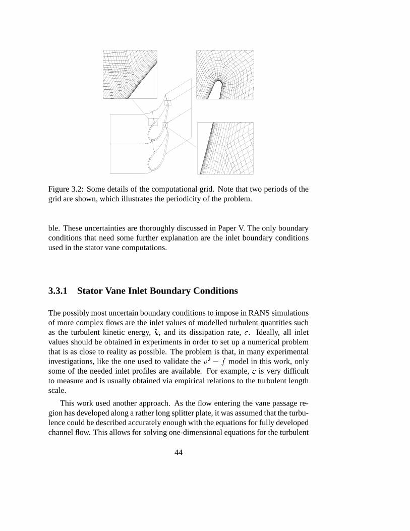
Figure 3.2: Some details of the computational grid. Note that two periods of thegrid are shown, which illustrates the periodicity of the problem.

ble. These uncertainties are thoroughly discussed in Paper V. The only boundaryconditions that need some further explanation are the inlet boundary conditionsused in the stator vane computations.

3.3.1 Stator Vane Inlet Boundary Conditions

The possibly most uncertain boundary conditions to impose in RANS simulationsof more complex flows are the inlet values of modelled turbulent quantities suchas the turbulent kinetic energy,

�, and its dissipation rate, � . Ideally, all inlet

values should be obtained in experiments in order to set up a numerical problemthat is as close to reality as possible. The problem is that, in many experimentalinvestigations, like the one used to validate the �

� � �model in this work, only

some of the needed inlet profiles are available. For example, � is very difficultto measure and is usually obtained via empirical relations to the turbulent lengthscale.

This work used another approach. As the flow entering the vane passage re-gion has developed along a rather long splitter plate, it was assumed that the turbu-lence could be described accurately enough with the equations for fully developedchannel flow. This allows for solving one-dimensional equations for the turbulent

44

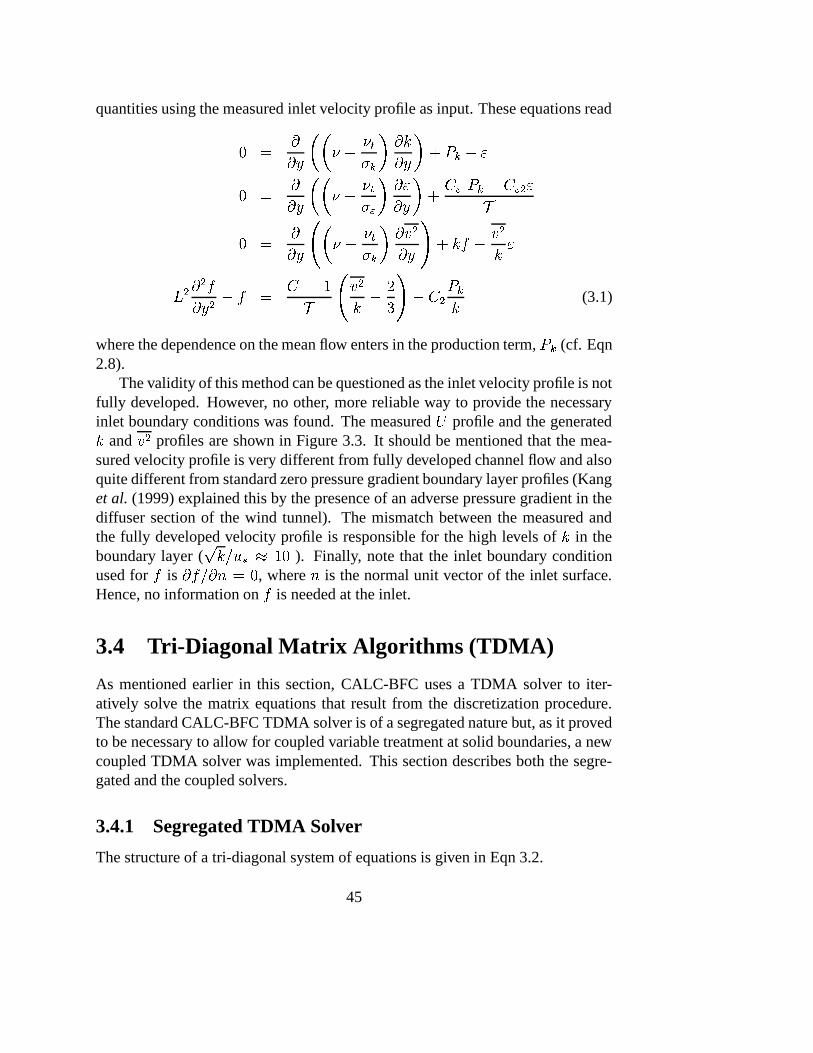
quantities using the measured inlet velocity profile as input. These equations read

� � �� : � � % �� : % � � � �

� � �� : � � % �� : % � � � � � � � � �7

� � �� : � � % ��

�� :�

% � � � � ��

� � � �� : � � � � � � �7 � � �� (3.1)

where the dependence on the mean flow enters in the production term,� �

(cf. Eqn2.8).

The validity of this method can be questioned as the inlet velocity profile is notfully developed. However, no other, more reliable way to provide the necessaryinlet boundary conditions was found. The measured

4profile and the generated�

and ��

profiles are shown in Figure 3.3. It should be mentioned that the mea-sured velocity profile is very different from fully developed channel flow and alsoquite different from standard zero pressure gradient boundary layer profiles (Kanget al. (1999) explained this by the presence of an adverse pressure gradient in thediffuser section of the wind tunnel). The mismatch between the measured andthe fully developed velocity profile is responsible for the high levels of

�in the

boundary layer (� � / � � � � ). Finally, note that the inlet boundary condition

used for�

is� � / � � � �

, where�

is the normal unit vector of the inlet surface.Hence, no information on

�is needed at the inlet.

3.4 Tri-Diagonal Matrix Algorithms (TDMA)

As mentioned earlier in this section, CALC-BFC uses a TDMA solver to iter-atively solve the matrix equations that result from the discretization procedure.The standard CALC-BFC TDMA solver is of a segregated nature but, as it provedto be necessary to allow for coupled variable treatment at solid boundaries, a newcoupled TDMA solver was implemented. This section describes both the segre-gated and the coupled solvers.

3.4.1 Segregated TDMA Solver

The structure of a tri-diagonal system of equations is given in Eqn 3.2.

45

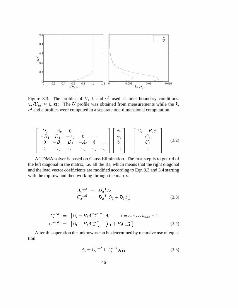
0 0.2 0.4 0.6 0.8 1 1.20

0.1

0.2

0.3

0.4

0.5

PSfrag replacements

��

�

0 0.005 0.01 0.015

PSfrag replacements

� ��

��

Figure 3.3: The profiles of4

,�

and ��

used as inlet boundary conditions.� � / 45��6 �� . The

4profile was obtained from measurements while the

�,

��

and � profiles were computed in a separate one-dimensional computation.

��

� � � � � ��

� � � ��

� �� ...

. . . . . . . . . . . . . . .

�� ...

��

�� % � � � � ��

�...

�� (3.2)

A TDMA solver is based on Gauss Elimination. The first step is to get rid ofthe left diagonal in the matrix, i.e. all the Bs, which means that the right diagonaland the load vector coefficients are modified according to Eqn 3.3 and 3.4 startingwith the top row and then working through the matrix.

�� % � � � �� (3.3)

�� ! � �� % � � � ��

�� (3.4)

After this operation the unknowns can be determined by recursive use of equa-tion

� � � � �� % � �� (3.5)

46

3.4.2 Coupled TDMA Solver

To enhance numerical stability it is sometimes beneficial to solve the equationscoupled. The coupled equations approach enables implicit formulation of, forexample, boundary conditions, where one flow field variable can be expressedin terms of another variable. An example is the boundary condition for

�in the

turbulence model suggested by Durbin (1995b)

�� : � � ��

(3.6)

In this expression for the wall value of�

we see a coupling with two other flowfield variables (if is a constant). When using the standard segregated approachwhere �

�and � have been recalculated separately a change in �

� / � is multipliedby a factor of

� �� /1: � . In the vicinity of wall boundaries the latter quantity isin my computations in the order of � � � and it is obvious that even a small changein �� / � undergoing this strong amplification can lead to oscillations, or worse,

divergence in the�

-equation.Now imagine that the �

�and�

sets of equations are combined into one systemof equations. This allows implicitly removing the sensitivity of

�at boundaries to

changes in ��

by adding coefficients in the left hand side matrix. The new, largermatrix is arranged as described in Eqn 3.7 (suggested by Eriksson (2002)) for aTDMA sweep in the

�-direction without introducing any coupling between �

�and�

(for definitions of coefficients � , � , . . . see Versteeg & Malalasekera (1995)).

��

� ��

� � � � � � � � � � � � � � � � � �� ...

. . . . . . . . . . . . . . . . . .

�� ...

��

� �� % � � � � �

�� $� �� % � ��

� � � �� ...

�� (3.7)

Now the�

boundary condition and the source term in the ��

equation canbe introduced implicitly. For example, if our

� � � boundary is a wall, we canimplement the boundary condition given by Eqn 3.6 by adding coefficient

��at

47

the matrix position giving the connection of the first interior�

value with the�

wall value. Implicit treatment of source term� � �

in the ��

equation correspondsto adding coefficient

�� . ��and

�� are given by Eqn 3.8

�� 8 �6 � � � � � � � 0 � 9 (3.8)

��

� �� ...

. . . . . . . . . . . . . . . . . .

�� ...

��

� �� % � � � � �

�� $� �� ...

�� (3.9)

This approach has two main disadvantages. The memory requirement in-creases as we must be able to handle matrices of size

� � �� ! by� � �� ! instead

of� � � ! by

� � � ! . The other drawback is that the matrix is now penta diagonal,which means that it is not possible to use a standard TDMA solver. Not muchcan be done to deal with the first problem, whereas it is fairly easy to rewrite aTDMA solver so that it can handle penta diagonal systems of equations. This isdone by changing the scalar coefficients in the standard TDMA matrix (Eqn 3.2)to two by two matrices and the unknown variable values and the load vector val-ues to vectors of two elements. In this way we get exactly the same structure ofthe TDMA matrix and can adopt the same solution methodology as for the scalar(special) case with the only difference that all operations are now matrix or vectoroperations. This is also the reason why, for example, � / � � in Eqn 3.3 is writtenin the more general form

� � � � . The arrangement of the coefficients for the newTDMA matrix equation is given in Eqn 3.10 and 3.11.

48

� � � � ��

� � � � � � � � � ��

� � � � � � � � ��

� � � � � � � � �� (3.10)

� � � ��

� � � (3.11)

3.5 Notes on the Commercial Software Used

Throughout the work here the computations made with the in-house code CALC-BFC have occasionally been complemented with computations performed withthe Fluent commercial software. There are several benefits in taking this approachand the effort needed to get acquainted with an additional software was consideredworthwhile. The complementary use of a commercial software allowed establish-ing a database with results for a wide range of commonly used turbulence models,whose implementations have been extensively benchmarked against experimentsin a wide range of flow conditions. Parts of this set of data have been publishedin Papers I & II to give an overview of the performance of different turbulencemodels in the flow considered. Another opportunity was the possibility to use anearly version of the �

� � �turbulence model that had been implemented in Fluent

by the use of so called User-Defined Functions (subroutines). The imlementationemployed was a trial version of the CASCADE Technologies Inc. V2F

��

modulefor Fluent 5. The use of this module allowed comparison of the results of exactlythe same turbulence model (the �

� � �model) on exactly the same computational

grid with exactly the same boundary conditions using two different CFD codes.The numerical features (e.g. solver and disctretization scheme) of the two codeswere chosen to be as equal as possible. Results of this comparison are also in-cluded in Papers I & II. The comparison would of course also instantly reveal anysevere error in the implementation of the �

� � �model in the CALC-BFC code.

A final purpose of using a commercial software was to increase the availabilityof recent progress in, for example, turbulence model development to the industrialpartners involved in this project. The reason behind industry’s dissatisfaction was

49

of course that any model development carried out within the project would not beavailable until the research community accepted the new ideas and the distributorsof the specific CFD code used implemented them in their software. And, whenfinally available, the ideas are also available to any competitor using the same soft-ware. To illustrate the potential of overcoming this problem using User-DefinedFunctions, a version of the �

� � �model was implemented in Fluent using this

approach and distributed to the partners involved.

50

Chapter 4

Summary of Papers

4.1 Paper I

This paper was based on a contribution to the 4��

International Symposium onTurbulence, Heat and Mass Transfer held in Antalya, Turkey, 2003. It was later,together with some 25 other contributions, selected for publication in an Int. Jour-nal of Heat and Fluid Flow Special Issue.

4.1.1 Background

Early in this project it was decided to implement the ��

model in the CFD codedescribed in Section 3 and evaluate its performance in a gas turbine stator vaneflow. The progress was initially very slow as it proved difficult to get the compu-tations with the new turbulence model running smoothly. As the respondent wasfairly new in the area of turbulence modelling it was hard to pinpoint the directcause of the problems encountered. Were they due to errors in the numerical grid?Or, which was more likely, errors in the implementation of the new model? Iteventually turned out to be neither of these candidates. Instead it was the formu-lation of the model itself that was not at all stable, at least not when used in theCALC-BFC framework. After about three months of debugging it was realizedthat the numerics could be substantially improved by avoiding the use of the real-izability constraint in the

�equation. The motivation for Paper I was therefore to

analyze why the realizability could have such a strong influence on the numericalproperties and, more importantly, how strongly the results of the �

� � �model

depend on the use of the same constraint. A second purpose was to compare twodifferent versions of the �

� � �model to see whether the modified version given

in e.g. Lien & Kalitzin (2001) gave the same results as the original version of the

51

model.

4.1.2 Discussion of Results

As mentioned, it was found that the use of the realizability constraint on the tur-bulence time scale can cause problems when used in the

�equation. The reason

was attributed to a positive feedback loop where a decrease in the time scale givenby the realizability constraint led to an increase in the modelled production of �

�,

which further reduced the upper bound on the time scale. Three alternative routesto using the realizability constraint in the

�and �

�equations, where one was not

to use it at all, were tested and all proved to improve the numerical stability ofthe model. It was also shown, by applying several modified formulations of therealizability constraint, that its use in the �

�and�

equations, at least in the flowcomputed, had only a minor influence on the converged solution.

Further, the effect of the model constant,� � � �

(cf. Eqn 2.43), introduced to-gether with the realizability constraint was investigated. By tuning this constantagainst measured turbulence kinetic energy profiles it was found that a value of0.6 gave the overall best agreement. This was very satisfying since this is thesame value that has been found suitable by other authors, which suggests someuniversality of this constant.

Finally, it was shown that the original version of the ��

model, i.e. theversion with the numerically cumbersome

�wall boundary condition, produced

the overall best agreement with experimentally obtained stator vane heat transferdata.

4.2 Paper II

This paper was based on a contribution to the TURBO EXPO Conference in Vi-enna, Austria, 2004. It was later, by people involved in the organization of theconference, recommended for publication in ASME Journal of Turbomachinery.

4.2.1 Background

The motivation for this paper is the true motivation as to why the stator vane flowwas to be computed with the �

� � �model in the first place (Paper I may be consid-

ered more of a side track). That is, we were interested in the model’s performancein a complex flow not too different from real flows found in gas turbine engines.Again, both versions of the �

� ��model were considered. A second objective

was to improve the understanding of the secondary flow mechanism responsible

52

for the strong increase in endwall heat transfer in the passage between two statorvanes. Also of interest was the response of the model’s heat transfer predictionsto increased levels of freestream turbulence. Two-dimensional midspan compu-tations were performed for this purpose. The evaluation was to be done by: i)comparing the computed results with experimental data of Kang & Thole (2000)and ii) comparing the models’ performance with that of turbulence models avail-able in the Fluent commercial software. At the time these computations wereperformed Fluent had just released a �

� ��module of their own that was made

available for testing at VAC.1 A problem with the module was that the details ofthat particular version of the �

� ��model were never given, which of course was

rather annoying, especially since there had been so many difficulties in getting themodel to work in the CALC-BFC code. Nevertheless, here was an opportunityto identify which version of the �

� � �model the Fluent module actually solved,

and to compare the performance of our in-house code with the commercial codeusing exactly the same grid and the same (?) turbulence model. Note that todayFluent give the details of the model they have implemented. They may be foundin Cokljat et al. (2003).


It was found that the two versions of the ��

model gave very similar re-sults, particularly in terms of predicting the secondary flow originating from thevane/endwall junction, known as the horseshoe vortex system. The �

� � �model

was found to be able to predict the presence of some of the vane passage vor-tices but in general gave somewhat too low intensities of the swirling motion ascompared with experimental data. A very close coupling between the endwallheat transfer and the secondary motion was illustrated. The heat transfer pre-dictions with both versions of the model responded fairly accurately to increasesin freestream turbulence intensity, with the original model performing somewhatbetter in the vane stagnation midspan region.

Of the models available in Fluent, the ��

model, followed by the RNG� � �

model, was found to give the best agreement with measurements. The poorest re-sults in terms of predicting the secondary flow were obtained with the Realizable� � � model. It was also found that the Fluent �

� ��version and the versions

implemented in CALC-BFC gave almost identical results, which was an encour-aging result. Further, it was illustrated that turbulence models without a fix for

1All the Fluent computations were performed at Volvo Aero Corporation, Trollh attan, Sweden,and the respondent wishes to acknowledge Dr. Jonas Larsson who made the time spent at VAC avery valuable experience.

53

the stagnation point anomaly, including the ��

with the realizability constraintdeactivated, suffer from massive overpredictions in stagnation point regions. Oneexample of a model that failed in this aspect was the Fluent implementation of theSST

� � � model. According to Dr. Fredrik Carlsson, Fluent, Sweden (privatecommunication), this problem has been dealt with in the latest version of Fluent.

Finally, the FLUENT predictions of the endwall stagnation region heat trans-fer were compared with experiments. All models gave similar estimates of theheat transfer in the region upstream of the vane. As the vane is approached, theinfluence of the horseshoe vortex, which significantly increases the heat transferto the endwall, is clear. It was found, however, that when the intensity of thepredicted vortex was close to the measured data the models tended to overpredictthe heat tranfer to the endwall. This, and the fact that the measured heat transfersignature of the vortex was not as clear in the experimental data as in the com-putations, suggests that the measured heat flux signal might have been affectedby heat leakage within the endwall or that the measured flow field was unsteady.Both phenomena would smear out the measured heat transfer profile.

Finally, the endwall stagnation region heat transfer results also suggest that themodel implemented in Fluent was very similar to the modified version of the �

� � �

model (the version with a stable�

wall boundary condition). The results of thesetwo implementations produced an almost perfect match, whereas the original �

� ��

model captures the heat transfer somewhat better.

4.3 Paper III

This paper is a modified and substantially extended version of a contribution to theTurbulence Shear Flow Phenomena in Williamsburg, USA, 2005, now submittedto the International Journal of Heat and Fluid Flow.

4.3.1 Background

Predicting separated flows with eddy-viscosity based closures is difficult. Onesuch flow that has been extensively studied is the asymmetric diffuser first con-sidered by Obi et al. (1993). The main reason why it is commonly used as atest case for turbulence models is its well-defined boundary conditions and its ap-parent simplicity. The flow physics is all but simple, however, and constitute anexceptionally difficult test case. In spite of the fact that the flow has been com-puted by a number of CFD researchers, the underlying reason as to why it is sodifficult to predict using RANS closures is not well understood. Some studieshave suggested that the near wall behavior is of great importance (e.g. Apsley &

54

Leschziner, 1999), which suggests that the ability of the ��

model to representnonlocal wall effects might be decisive. The main purpose of this study was toshed additional light on the subject and to identify the flow features that are ofdynamic importance. The LES data of Kaltenbach et al. (1999) were used forvalidation purposes.

Even though the ��

model has shown promising results in this flow, it isin principle unable to account for turbulence anisotropy. It was therefore decidedto investigate the performance of the nonlinear extension to the �

� ��model

suggested by Pettersson-Reif (2000). Note that the nonlinear model has provedcapable of accurate predictions of anisotropy driven effects and that it is of interestto investigate whether the extended model still performs as well in separated flowsas the less sophisticated linear model.


This study showed that the dynamically most important flow region is the nearwall region in close vicinity to the diffuser entrance. Here exists a delicate bal-ance between the Reynolds stresses and it is required that the evolution of all threecomponents ( � � � , � � � and � � � ) is correctly modelled. Several interesting ob-servations were made. One was that the reason why the linear �

�� model gets

this flow about right is not that it is particularly good, but rather that it producestwo errors that happen to cancel each other. Another was that the nonlinear �

� � �

model, at least in the beginning of the diffuser, did a very good job in representingthe complex flow anisotropy, but did substantially worse than the linear model interms of mean velocity profiles. The reason for this puzzling result turned out tobe that one of the errors the linear model produced was improved a great deal withthe consequence that the other error was left unbalanced.

It was also shown that the performance of the nonlinear model could be im-proved with a slight modification of the

� � coefficient. This modification seemedalso to fix the unbalanced error. It could therefore also be concluded that the non-linear constitutive equation suggested by Pettersson-Reif (2000) is sufficiently ac-curate for the purpose of computing the complex flow field in the asymmetricdiffuser.

The effect of a more elaborate turbulence diffusion model in the�

and � equa-tions was also tested, and the results seem to suggest that the turbulence transportmodel does not play a primary role in this particular flow and that the

�and �

equations are dominated by their source terms.A final conclusion was that the flow in the asymmetric diffuser, at least in the

first half of the diffusing section, is largely of a parabolic nature. A consequenceis that errors in the early part of the diffuser rather severely affect the flow de-

55

velopment in downstream portions of the diffuser. It seems thus to be of littlevalue to optimize a turbulence model to perform well in the separated region ofthe diffuser if the upstream flow is not correctly captured.

4.4 Papers IV and V

4.4.1 Motivation

The ��

model, as almost every other turbulence model, is known to predicttransition too early. Therefore, in an effort to increase the �

� � �model’s reliability

as a gas turbine design tool, the overall aim of Papers IV-V was to identify ameasure to improve its performance in transitional flows.

Paper IV is a review of transitional modelling that includes a variety of ap-proaches to the problem suggested in the second half of the 20th century. Asby-pass transition is probably the transition mode that suits a statistical modellingapproach best, this mode, and its modelling, is the one that is most thoroughlydiscussed. Included are also the latest findings on the nature of by-pass transition.The main purpose of the review was to search the existing literature for a mod-elling approach that could be coupled to the, in fully turbulent flows, reasonblyaccurate �

� � �turbulence model. A second purpose was of course to provide a

reference text where most relevant earlier work on the subject is collected.


It was decided to adopt the modelling concept of Mayle & Schultz (1997), refinedby Walters & Leylek (2004), i.e. to introduce an additional transport equationgoverning the evolution of a laminar kinetic energy. It is well known that streaksof laminar � -component fluctuations are somehow created in the pretransitionalboundary layer and that these streaks are precursors to the formation of turbulentspots. It was thus believed that modelling statistics of these streaks (their fluctuat-ing energy) would be an approach to modelling transitional phenomena that stoodon a reasonably firm ground. The coupling of most of the concepts introducedby Walters & Leylek (2004) with a modified version of the �

� � �model is what

Paper V is about.This work has led to the conclusion that the model of Walters & Leylek (2004)

is very sensitive; the freestream turbulence length scale and a few of their conceptshave to be reconsidered.

56

Chapter 5

Concluding Remarks

This thesis has dealt with the closure, or modelling, of turbulence transport effectson averaged flow properties of turbulent flows. The main applications have allbeen related to turbomachinery components with a focus on flow or modellingfeatures particularly important to heat transfer in gas turbine engines. The mostimportant findings will be given below in three separate sections. Section 5.1summarizes the results of the two and three-dimensional computations reportedin Papers I & II. Also included in this section are the results of the realizabilityconstraint study and a few comments on the present computational approach ingeneral. Section 5.2 gives some comments on the potential of using nonlineareddy-viscosity models together with findings on the subtle subject of turbulencemodelling in separating flows. Section 5.3 is a summary of the conclusions drawnin the effort to improve the transition modelling capability of the �

� � �turbulence

model. The final section contains some guidelines for future work in the area ofturbulence modelling for gas turbine applications.

5.1 Stator Vane Passage Flows

Two-dimensional Passage Flow Computations

All computations of the two-dimensional stator vane flow produced attached ve-locity fields with very small overall differences in behavior among the differ-ent turbulence models investigated. The largest differences are found within theboundary layers. More specifically, the flow property that differs the most is thelocation of transition onset. It was found that no model was able to predict the on-set location but, by judging the performance in terms of heat transfer predictions,the �

� � �model of Durbin (1995b) must be regarded as the most reliable model.

57

In stagnation point flows it is important that the model used for turbulence clo-sure is able to handle the so called stagnation point anomaly (large overpredictionof turbulence kinetic energy). Models that do not handle this problem predict toohigh heat transfer rates and the elevated levels of turbulence tend also to acceleratethe laminar to turbulence transition process. It was found that an efficient way toreduce the erroneous growth of fluctuating energy was to employ the realizabilityconstraint of Durbin (1995a). However, this constraint, when expressed in termsof an upper bound on the turbulence time scale, proved to destabilize the path to aconverged solution. A mechanism behind the instabilities was suggested togetherwith some alternative ways to employ the constraint that all improved the numer-ical stability. The most straightforward alternative to reduce the overprediction ofturbulent kinetic energy is simply to express the constraint in terms of a bound onthe predicted eddy-viscosity.

Three-dimensional Passage Flow Computations

The three-dimensional computations of the stator vane passage flow illustrated thecrucial dependence of endwall heat transfer on the secondary flow structures ema-nating from the stator vane/endwall junction. The origin of these so called horse-shoe vortices is the vorticity contained in the oncoming boundary layer. In theflow computed, the boundary layer is thick, which causes strong secondary mo-tions. It therefore turned out that accurately capturing the roll-up of these vorticesis particularly important. The presence of this vortex causes the relatively thickoncoming boundary layer to separate from the endwall. This is unfortunate sincethe boundary layer fluid should act as an insulating layer, protecting the endwallfrom the hot freestream fluid. The vortex also effectively replaces the boundarylayer fluid (that separated from the endwall) with hot fluid from the freestreamthat, owing to the rotating motion of the vortex, impinges on the endwall surfacewhich severely increases the rate of heat transfer to the endwall.

The results thus indicate that the endwall heat transfer rate primarily dependson a correct prediction of the secondary flow structures present. Of secondaryimportance is the prediction of the heat transfer due to turbulence1. However, ofcrucial importance is the effect of turbulence on the secondary flow field. Thatis, if for some reason the predicted effect of turbulence erroneously affects thesecondary motion, this error will also ruin the heat transfer prediction in the vanepassage.

Of the different turbulence models investigated, the two versions of the ��

model tested performed better than the turbulence closures available in the Fluent

1This was also verified by varying the inlet turbulence boundary conditions which only slightlymodified the computed heat transfer data.

58

commercial software with the possible exception of the RNG� � � model. It was

also found that the in-house CALC-BFC code and the trial version of a ��

module (cf. Section 3.5) implemented with User-Defined Functions gave iden-tical results. That is, with the same turbulence model, the same numerical gridand boundary condition, CALC-BFC and Fluent give identical results. Finally,of the two versions of the �

� � �model tested in this flow, the version in Durbin

(1995b) did somewhat better in terms of heat transfer, a trend also seen in thetwo-dimensional vane computations. Both models, however, perform less satis-factorily, as compared with the results in the stagnation region, some distance intothe stator vane passage. It is believed that this is due to an inaccurate representa-tion of the secondary vortices as they are convected through the vane passage. Inall computations the intensity of the secondary motions and the net flow towardsthe suction side of the adjacent stator vane were underpredicted.

All ��

model computations performed with the in-house CALC-BFC codewere problematic from a numerical stability point of view. The main source of in-stability is believed to be the

�equation, which is an equation of an elliptic nature

describing the evolution of a turbulence quantity with large source terms creatinga strong coupling to other turbulence quantities. There is thus room for oscilla-tions not seen in the other turbulence equations that are not convected through thenumerical domain.

In the computations made with the Durbin (1995b) model the stability prob-lems were even worse owing to the extremely strong coupling of the

�wall bound-

ary condition to other near wall turbulence quantities. These computations werenever even close to converging without the use of the coupled TDMA solver de-scribed in Section 3.4.22. With the coupled solver the stability of the Durbin(1995b) model was improved and the code behaved as when the modified morestable version of the �

� � �model was used. There was initially some hope that

the coupled solver would also improve the stability of the code-friendly versionof the �

� ��model, as this solver allows implicit treatment of the �

�equation

source term (� �

) and the�

equation sink term (� � ), but no conclusions on de-

cisive improvements could be drawn. It is interesting to note, however, that thecode-friendly version of the �

� � �model seems not to have any additional nu-

merical difficulties, as compared with other turbulence models available, whenimplemented in Fluent.

2This model was also implemented in Fluent (version 6.2.16) using User-Defined Functionsand did, after considerable effort, produce a converged solution for a one-dimensional, fully de-veloped channel flow computation. The stability seems however not to be significantly better thanwith the CALC-BFC solver.

59

5.2 Separation in the Asymmetric Diffuser

The linear ��

model is argued to be among the better models in flows involv-ing separation. It is however unable to make correct representations of turbulenceanisotropy. In this study the potential of using a nonlinear eddy-viscosity turbu-lence model was therefore investigated. The model tested was the nonlinear ex-tension to the �

� � �model suggested by Pettersson-Reif (2000). When compared

with the linear version of the model, all the components of the Reynolds stress ten-sor, and especially its normal components, were substantially improved in almostthe entire numerical domain. On the other hand, the prediction of the mean flowwas worse than with the linear model. This somewhat surprising finding, giventhe quality of the Reynolds stresses, could be explained in a careful analysis ofthe momentum equation source terms, i.e. the Reynolds stress derivatives, in theclose vicinity of the curved wall in the diffuser entrance region. Here a delicatebalance between the Reynolds stresses exists and it turned out that the reason whythe linear model produced results in close agreement with LES data was that twoerrors of equal magnitude cancelled each other. The nonlinear extension provedto solve one of the two problems, which left the other error unbalanced.

A few modifications to the nonlinear model were preliminarily assessed in aneffort to further improve its performance. All modifications involved changes ofthe � equation coefficient

� � , which controls the production rate of � . One of themodifications tested was found to significantly improve the model performance inthe diffuser entrance and also improved the predicted mean velocity field. Thismodification reduced the unbalanced near wall error mentioned above, which fur-ther supports our reasoning that the near wall behavior is of utmost importance tothe flow in the diffuser.

Finally, it was concluded that the choice of diffusion model for the turbulencekinetic energy and its dissipation rate was of subordinate importance and, thus,that these equations are dominated by their source terms in the asymmetric dif-fuser flow.

5.3 Transition

The subject of transition modelling was reviewed in Paper IV. The main purposeof that study was to examine existing ideas and to find a basis for extending thecapabilities of the �

� � �model to also include transitional flows. After consider-

ing a few concepts in more detail it was decided to adopt the modelling frameworksuggested by Walters & Leylek (2004). Here an additional transport equation for alaminar kinetic energy is solved together with a typical turbulence model. Walters

60

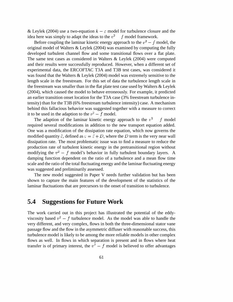
& Leylek (2004) use a two-equation� � � model for turbulence closure and the

idea here was simply to adapt the ideas to the ��

model framework.Before coupling the laminar kinetic energy approach to the �

� � �model, the

original model of Walters & Leylek (2004) was examined by computing the fullydeveloped turbulent channel flow and some transitional flows over a flat plate.The same test cases as considered in Walters & Leylek (2004) were computedand their results were successfully reproduced. However, when a different set ofexperimental data, the ERCOFTAC T3A and T3B test cases, was considered itwas found that the Walters & Leylek (2004) model was extremely sensitive to thelength scale in the freestream. For this set of data the turbulence length scale inthe freestream was smaller than in the flat plate test case used by Walters & Leylek(2004), which caused the model to behave erroneously. For example, it predictedan earlier transition onset location for the T3A case (3% freestream turbulence in-tensity) than for the T3B (6% freestream turbulence intensity) case. A mechanismbehind this fallacious behavior was suggested together with a measure to correctit to be used in the adaption to the �

� � �model.

The adaption of the laminar kinetic energy approach to the ��

modelrequired several modifications in addition to the new transport equation added.One was a modification of the dissipation rate equation, which now governs themodified quantity

�� , defined as � � �� % , where the term is the very near walldissipation rate. The most problematic issue was to find a measure to reduce theproduction rate of turbulent kinetic energy in the pretransitional region withoutmodifying the �

� � �model’s behavior in fully turbulent boundary layers. A

damping function dependent on the ratio of a turbulence and a mean flow timescale and the ratio of the total fluctuating energy and the laminar fluctuating energywas suggested and preliminarily assessed.

The new model suggested in Paper V needs further validation but has beenshown to capture the main features of the development of the statistics of thelaminar fluctuations that are precursors to the onset of transition to turbulence.

5.4 Suggestions for Future Work

The work carried out in this project has illustrated the potential of the eddy-viscosity based �

� ��turbulence model. As the model was able to handle the

very different, and very complex, flows in both the three-dimensional stator vanepassage flow and the flow in the asymmetric diffuser with reasonable success, thisturbulence model is likely to be among the more reliable models in other complexflows as well. In flows in which separation is present and in flows where heattransfer is of primary interest, the �

��model is believed to offer advantages

61

over other eddy-viscosity based closures.There appears, however, to exist two weaknesses in the model. It is more or

less unable to account for turbulence anisotropy and predicts the onset of transitionto occur too early. Both problems have been addressed in this thesis. The non-linear extension to the �

� � �model appears to offer substantial improvements in

the representation of turbulence anisotropy. However, two important weaknessessof the nonlinear model have been pinpointed and need further attention. One isthe modelling of the dissipation rate equation. A modification that improved themodel’s performance has beed suggested but needs to be more extensively testedin other applications. The other is that the nonlinear terms added tend to makethe model numerically unstable. A continuation of the development of the non-linear model will therefore require implementation of state-of-the-art numericalmethods to increase the model’s reliability.

The subject of transition is of crucial importance to the design of turbomachin-ery components, especially those for which heat transfer is of primary importance,and cannot be neglected. The effort described here to improve the �

� � �model’s

performance in transitional flows needs further work on both model developmentand validation. Of the two ‘missing links’, that of transition is by far the mostimportant to turbomachinery design.

62

Bibliography

ABE, K., KONDOH, T. & NAGANO, Y. 1994 A new turbulence model for pre-dicting fluid flow and heat transfer in separating and reattaching flows–1. Flowfield calculations. Int. J. of Heat and Mass Transfer 37, 139–151.

APSLEY, D. & LESCHZINER, M. 1999 Advanced turbulence modelling of sepa-rated flow in a diffuser. Flow, Turbulence and Combustion 63, 81–112.

BATCHELOR, G. K. 1967 An introduction to fluid dynamics. Cambridge Univer-sity Press.

BOYLE, R. & RUSSELL, L. 1990 Experimental determination of stator endwallheat transfer. Journal of Turbomachinery 112, 547–558.

BRADSHAW, P. 1996 Turbulence modelling with application to turbomachinery.Proc. Aerospace Science 32, 575–624.

COKLJAT, D., KIM, S., IACCARINO, G. & DURBIN, P. 2003 A comparativeassessment of the �

� � �model for recirculating flows. AIAA-2003-0765.

CRAFT, T. J. 2002 Modelling of separating and impinging flows. In ClosureStrategies for Turbulent and Transitional Flows (ed. B. E. Launder & N. D.Sandham), pp. 341–360. Cambridge University Press.

DALY, B. J. & HARLOW, F. H. 1970 Transport equations in turbulence. Interna-tional Physics of Fluids 13, 2634–2649.

DAVIDSON, L. & FARHANIEH, B. 1995 CALC-BFC: A finite-volume code em-ploying collocated variable arrangement and cartesian velocity components forcomputation of fluid flow and heat transfer in complex three-dimensional ge-ometries. Rept. 95/11. Dept. of Thermo and Fluid Dynamics, Chalmers Univer-sity of Technology, Gothenburg.

63

DUNN, M. 1990 Phase and time-resolved measurements of unsteady heat transferand pressure in a full-stage rotating turbine. Journal of Turbomachinery 112,531–538.

DUNN, M., RAE, W. & HOLT, J. 1984 Measurement and analyses of heat fluxdata in a turbine stage: Part ii—discussion of results and comparison with pre-dictions. Journal of Engineering for Gas Turbines and Power pp. 234–240.

DURBIN, P. 1991 Near-wall turbulence closure modeling without ’damping func-tions’. Theoretical and Computational Fluid Dynamics 3, 1–13.

DURBIN, P. 1993 Application of a near-wall turbulence model to boundary layersand heat transfer. International Journal of Heat and Fluid Flow 14, 316–323.

DURBIN, P. 1995a On the� � � stagnation point anomaly. International Journal

of Heat and Fluid Flow 17, 89–90.

DURBIN, P. 1995b Separated flow computations with the� � � � � � model. AIAA

Journal 33, 659–664.

ERIKSSON, L. 2002 private communication. Dept. of Thermo and Fluid Dynam-ics, Chalmers University of Technology, G oteborg, Sweden.

GIEL, P., FOSSEN, R. V., BOYLE, R., THURMAN, D. & CIVINSKAS, K. 1999Blade heat transfer measurements and predictions in a transonic turbine cas-cade. NASA/TM—1999-209296.

GIEL, P., THURMAN, D., FOSSEN, R. V., HIPPENSTEELE, S. & BOYLE, R.1998 Endwall heat transfer measurements in a transonic turbine cascade. Jour-nal of Turbomachinery 120, 305–313.

GIEL, P., THURMAN, D., LOPEZ, I., BOYLE, R., FOSSEN, R. V., JETT, G.,CAMPERCHIOLI, T. & LA, H. 1996 Three-dimensional flow field measure-ments in a transonic turbine cascade. ASME paper No. 96-GT-113 .

GRAZIANI, R., BLAIR, M., TAYLOR, J. & MAYLE, R. 1980 An experimentalstudy of endwall and airfoil surface heat transfer in a large scale turbine bladecascade. Journal of Engineering for Power 102, 257–267.

HARVEY, N., ROSE, M., COUPLAND, J. & JONES, T. 1999 Measuremementand calculation of nozzle guide vane end wall heat transfer. Journal of Turbo-machinery 121, 184–190.

64

HERMANSON, K. & THOLE, K. 2000a Effect of inlet conditions on endwallsecondary flows. Journal of Propulsion and Power 16, 286–296.

HERMANSON, K. & THOLE, K. 2000b Effect of Mach number on secondary flowcharacteristics. International Journal of Turbo and Jet Engines 17, 179–196.

JOHANSSON, G. & KLINGMANN, J. 1994 An LDA based method for accuratemeasurements of the dissipation rate tensor with application to a circular jet. In7th Int. Symp. on Applications of Laser Techniques to Fluid Mechanics. Lisbon.

JOHANSSON, T. 2002 private communication. Dept. of Thermo and Fluid Dy-namics, Chalmers University of Technology, G oteborg, Sweden.

JONES, W. & LAUNDER, B. 1972 The prediction of laminarization with a two-equation model of turbulence. Int. J. of Heat and Mass Transfer 15, 301–314.

KALITZIN, G. 1999 Application of the ��

model to aerospace configurations.Center for Turbulence Research Annual Research Breifs.

KALTENBACH, H., FATICA, M., MITTAL, R., LUND, T. & MOIN, P. 1999 Studyof flow in a planar asymmetric diffuser using large-eddy simulation. Journal ofFluid Mechanics 390, 151–185.

KANG, M., KOHLI, A. & THOLE, K. 1999 Heat transfer and flowfield measure-ments in the leading edge region of a stator vane endwall. Journal of Turboma-chinery 121, 558–568.

KANG, M. & THOLE, K. 2000 Flowfield measurements in the endwall region ofa stator vane. Journal of Turbomachinery 122, 458–466.

KATO, M. & LAUNDER, B. 1993 The modelling of turbulent flow around sta-tionary and vibrating square cylinders. In Ninth Symposium on Turbulent ShearFlows, pp. 10–4–1–10–4–6.

LANGSTON, L., NICE, M. & HOOPER, R. 1977 Three-dimensional flow withina turbine cascade passage. Journal of Engineering for Power 99, 21–28.

LAUNDER, B., REECE, J. & RODI, W. 1975 Progress in development of aReynolds-stress turbulence closure. Journal of Fluid Mechanics 68, 537–566.

LIEN, F. & KALITZIN, G. 2001 Computations of transonic flow with the ��-�

turbulence model. International Journal of Heat and Fluid Flow 22, 53–61.

65

MANCEAU, R., WANG, M. & LAURENCE, D. 2001 Inhomogeneity and isotropyeffects on the redistribution term in Reynolds-Averaged Navier-Stokes mod-elling. Journal of Fluid Mechanics 438, 307–338.

MAYLE, R. & SCHULTZ, A. 1997 The path to predicting bypass transition. Jour-nal of Turbomachinery 119, 405–411.

MENTER, F. 1993 Zonal two equation� � � turbulence models for aerodynamic

flows. Tech. Rep.. Eloret Institute, Sunnyvale, CA.

MENTER, F., KUNTZ, M. & LANGTRY, R. 2003 Ten years of industrial expe-rience with the SST

� � � � � � � � � � � � � �� . In 4th Int. Symp. on TurbulenceHeat and Mass Transfer. Antalya, Turkey.

MORAN, A. G. B. 2004 Prediction of the axisymmetric impinging jet with dif-ferent

� � � turbulence models. Report 04/29. Dept. of Thermo and Fluid Dy-namics, Chalmers University of Technology, G oteborg, Sweden, mSc Thesis.

MOSER, R., KIM, J. & MANSOUR, N. 1999 Dns of turbulent channel flow up tore �

��. Physics of Fluids 11, 943–945.

NARASIMHAMURTHY, V. D. 2004 Unsteady-rans simulation of turbulent trailing-edge flow. Report 04/31. Dept. of Thermo and Fluid Dynamics, Chalmers Uni-versity of Technology, G oteborg, Sweden, mSc Thesis.

NILSSON, H. 2002 Numerical investigations of turbulent flow in water turbines.PhD thesis, Dept. of Thermo and Fluid Dynamics, Chalmers University ofTechnology, G oteborg, Sweden.

OBI, S., AOKI, K. & MASUDA, S. 1993 Experimental and computational studyof turbulent separating flow in an asymmetric plane diffuser. In Ninth Sympo-sium on Turbulent Shear Flows, Kyoto, Japan, p. 305.

PATEL, C., RODI, W. & SCHEUERER, G. 1985 Turbulence models for near-walland low Reynolds number flows: A review. AIAA Journal 23, 1308–1319.

PETTERSSON-REIF, B. A. 2000 A nonlinear eddy-viscosity model for near-wallturbulence. AIAA paper 2000-0135.

PHILLIPS, O. M. 1969 Shear-flow turbulence. Annual Review of Fluid Mechanics1, 245–264.

POPE, S. B. 1975 A more general eddy-viscosity hypothesis. Journal of FluidMechanics 72, 331–340.

66

RADOMSKY, R. 2000 High freestream turbulence studies on a scaled-up statorvane. PhD thesis, University of Wisconsin-Madison.

RADOMSKY, R. & THOLE, K. 2000 Measurements and predictions of a highlyturbulent flowfield in a turbine vane passage. Journal of Fluids Engineering122, 666–676.

RUBENSDORFFER, F. 2002 Literature survey: Vane and blade secondary flow andendwall heat transfer. Rept. kth-hpt-37/02. Dept. of Energy Technology, RoyalInsitue of Technology, Stockholm.

SHARMA, O. & BUTLER, T. 1987 Predictions of endwall losses and secondaryflows in axial flow turbine cascades. Journal of Turbomachinery 109, 229–236.

SIEVERDING, C. 1985 Recent progress in the understanding of basic aspect ofsecondary flows in turbine blade passages. Journal of Engineering for Gas Tur-bines and Power 107, 248–257.

SIMONEAU, R. & SIMON, F. 1993 Progress towards understanding and predict-ing heat transfer in the turbine gas path. International Journal of Heat and FluidFlow 14, 106–128.

SPENCER, M. & JONES, T. 1996 Endwall heat transfer measurements in an annu-lar cascade of nozzle guide vanes at engine representative Reynolds and Machnumbers. Journal of Heat and Fluid Flow 17, 139–147.

SVENINGSSON, A. 2003 Analysis of the performacne of different ��

turbu-lence models in a stator vane passage flow. Licentiate thesis. Dept. of Thermoand Fluid Dynamics, Chalmers University of Technology, Gothenburg, Swe-den.

SVENINGSSON, A. & DAVIDSON, L. 2004 Computations of flow field and heattransfer in a stator vane passage using the �

� ��turbulence model. In ASME

Turbo Expo 2004. To appear in conference publication. Vienna, Austria.

SVENINGSSON, A. & DAVIDSON, L. 2005 Computations of flow field and heattransfer in a stator vane passage using the �

�-�

turbulence model. Journal ofTurbomachinery 127, 627–634.

THOLE, K., RADOMSKY, R., KANG, M. & KOHLI, A. 2002 Elevated freesteamturbulence effects on heat transfer for a gas turbine vane. International Journalof Heat and Fluid Flow 23, 137–147.

67

VERSTEEG, H. & MALALASEKERA, W. 1995 An Introduction to ComputationalFluid Dynamics. Addison Wesley Longman Ltd.

WALTERS, D. & LEYLEK, J. 2004 A new model for boundary layer transitionusing a single-point rans approach. Journal of Turbomachinery 126, 193–202.

WILCOX, D. 1993 Turbulence Modeling for CFD. Griffin Printing, Glendale.

68

turbulence transport modelling in gas turbine related applications

Documents