understanding ecohydrological connectivity in savannas… · understanding ecohydrological...

ECOHYDROLOGYEcohydrol.Published online in Wiley Online Library(wileyonlinelibrary.com) DOI: 10.1002/eco.245

Understanding ecohydrological connectivity in savannas:a system dynamics modelling approach

Gretchen R. Miller,1* Jessica M. Cable,2 Alyson K. McDonald,3 Barbara Bond,4

Trenton E. Franz,5 Lixin Wang,5,6 Si Gou,1 Anna P. Tyler,7 Chris B. Zou8 and Russell L. Scott9

1 Department of Civil Engineering, Texas A&M University, College Station, TX, USA2 International Arctic Research Center, University of Alaska, Fairbanks, AK, USA

3 Department of Ecosystem Science and Management, Texas AgriLife Extension Service, Texas A&M University, Fort Stockton, TX, USA4 Department of Forest Ecosystems and Society, Oregon State University, Corvallis, OR, USA

5 Department of Civil and Environmental Engineering, Princeton University, Princeton, NJ, USA6 School of Civil and Environmental Engineering, University of New South Wales, Sydney, NSW, Australia

7 Department of Ecology and Evolutionary Biology, University of Arizona, Tucson, AZ, USA8 Department of Natural Resource, Ecology and Management, Oklahoma State University, Stillwater, OK, USA

9 Southwest Watershed Research Center, Agricultural Research Service, USDA, Tucson, AZ, USA

ABSTRACT

Ecohydrological connectivity is a system level property that results from the linkages in the networks of water transport throughecosystems, by which feedbacks and other emergent system behaviours may be generated. We created a system dynamicsmodel that represents primary ecohydrological networks to examine how connectivity between ecosystem components impactsecosystem processes. Here, we focused on the savanna ecosystems, although the analyses may be expanded to other ecosystemtypes in the future. To create the model, a set of differential equations representing ecohydrological processes was programmedinto the dynamic solver Vensim. Stocks of water storage (e.g. atmospheric and soil moisture) were linked by flows [e.g.precipitation and evapotranspiration (ET)] that were in turn dynamically controlled by the amount of water stored. Precipitationwas forced stochastically, and soil moisture and potential ET controlled actual ET. The model produced extended, probabilistictime series of stocks and flows, including precipitation, soil moisture, runoff, transpiration, and groundwater recharge. It wasused to describe the behaviour of several previously studied savanna ecosystems in North America and Africa. The modelsuccessfully reproduced seasonal patterns of soil moisture dynamics and ET at the California site. It also demonstrated morecomplex, system level behaviours, such as multiyear persistence of drought and synergistic or antagonistic responses todisconnection of system components. Future improvements to the model will focus on capturing other important aspects oflong-term system behaviour, such as changes in physiology or phenology, and spatial heterogeneity, such as the patchworknature of savannas. Copyright 2011 John Wiley & Sons, Ltd.

KEY WORDS cross-scale interactions; feedbacks; resilience; disturbance; system dynamics; soil moisture dynamics;evapotranspiration

Received 25 August 2010; Accepted 26 May 2011

INTRODUCTION

The ‘connectivity’ between components of an ecosys-tem influences overall system function and stability. Theconcept of ecosystem connectivity originated with stud-ies in animal population dynamics in the 1970s, whereit represents the ‘degree to which the landscape facil-itates or impedes movement among resource patches’(Tischendorf and Fahring, 2000). In other disciplines,connectivity has been defined and utilized inconsistently(Calabrese and Fagan, 2004), as it has been used todescribe processes related to both structure and functionof landscapes (Tischendorf and Fahring, 2000). We sug-gest that connectivity is a system level characteristic thatdescribes networks of a medium or transport vectors, suchas wind, water, and animals, which link patchworks of

* Correspondence to: Gretchen R. Miller, Department of Civil Engineer-ing, Texas A&M University, College Station, TX, USA.E-mail: [email protected]

resources or organisms. Connectivity essentially resultsfrom a network–patchwork association.

More recently, the concept of connectivity has beenapplied to physical (soil) and biological (plant) processeswithin and across ecosystems, specifically the exchangeof matter and energy at multiple temporal and spatialscales (Peters et al., 2006). Connectivity can occur inthe vertical or horizontal plane and there may be avariety of connecting media. In semi-arid ecosystems,water is the primary medium of connectivity because itcontrols physical and biological processes across scales(Austin et al., 2004; Wang et al., 2009). Rates of move-ment and exchange of water depend upon the char-acteristics and connectivity of pathways, such as thesoil–plant–atmosphere continuum (vertical connectiv-ity), soil properties (both vertical and horizontal connec-tivity), and the distribution of plants on the landscape(horizontal connectivity), as shown in Figure 1.

Quantifying connectivity can be challenging, and evi-dence of connectivity is clear in some situations but

Copyright 2011 John Wiley & Sons, Ltd.

5, 200–220 (2012) 7 July 2011

Figure 1. A conceptual diagram depicting the horizontal and vertical connectivity of an ecosystem with water as the primary medium. The poolsbetween which the water is moving include different layers of soil, vegetation, and atmosphere. The vertical connections occur at several levels. Thefirst is the upward movement of water via the soil–plant–atmosphere continuum (plant transpiration, evaporation from soil, and plant interception)or just the soil–atmosphere continuum (soil evaporation). The second is downward movement of water in the soil via infiltration of rainfall, waterexfiltration, percolation, and recharge. The horizontal connections occur on the soil surface as overland flow and in subsurface layers as lateral flow.

only suggestive in others. Adding to the complexity,connectivity can be cyclic or unidirectional. Rainfallrecycling from evapotranspiration (ET) is an exampleof cyclic connectivity, where the connection betweenwater in the soil, plants, and the atmosphere results inwater retention within the system (Richards and Cald-well, 1987; Sala et al., 1989; Dawson and Ehleringer,1991; Trenberth, 1999). A clear example of unidirec-tional connectivity is overland water flow, or run-on andrunoff, where water moves downslope and redistributesto a different location, such as a depression or vegetatedpatch (Reid et al., 1999; Dunkerley, 2002; Ludwig et al.,2005), and transports with it soil nutrients in the formof litter or dissolved inorganic chemicals (Belnap et al.,2005; Wang et al., 2011).

Modelling connectivity at the ecosystem level is also acomplex problem, largely due to cross-scale interactions(Peters et al., 2008) and the ‘paradox of scale’ (Wilcoxet al., 2006), wherein organ-, organism-, or plot-levelprocesses tend not to scale to the ecosystem level. Thissuggests that whole ecosystems behave differently—withregard to controls over water and carbon fluxes—thanthe sum of the individual parts (Osmond et al., 2004).Thus, small-scale measurements are not likely to cap-ture the connectivity occurring on different temporal andspatial scales. Time lags in plot- or leaf-level processescan create temporal discontinuities, while variations inmicro-scale soil texture, interplant variability, and patch-iness in soil microbial distributions can induce spatialdifferences. Essentially, by capturing spatial and/or tem-poral ‘snapshots’ of physical and biological activitiesvia spot measurements, the connectivity between differ-ent ecosystem components is likely to be missed, andthe network–patchwork dynamic of fluxes will not be

captured. This limits our ability to predict how broadchanges in climate or land use may impact ecosystemprocesses (Tang and Bartlein, 2008).

A more robust understanding of ecosystem connec-tivity may contribute to predicting the effects of envi-ronmental change, from land use to climate change, onecosystems. For example, there may be an optimum leveland type of connectivity that creates resilience and sta-bility in ecosystem function (Haydon, 2000; Sole andMontoya, 2001; Peters et al., 2004). Loss or creationof connectivity could lead to state transition (Briskeet al., 2005). Widespread shrub encroachment into grass-lands (Schlesinger et al., 1990; Archer, 1994; Van Auken,2000) is a significant example of a change in connec-tivity. The resulting fragmentation of grasslands causesa shift from a homogeneous to heterogeneous distri-bution of water and soil nutrients, whereby resourcesbecome concentrated around woody plants (‘islands offertility’), leaving exposed soil in adjacent interspacesformerly occupied by grasses (Schlesinger et al., 1990;Bhark and Small, 2003; Okin et al., 2009; Ravi et al.,2010). This ‘patchiness’ also drives spatial variation insoil and ecosystem processes, and can decouple ecosys-tem processes, such as plant production, from climatedrivers, such as precipitation (Scott et al., 2006).

Savanna ecosystems occur in semi-arid climates andare ecotones that have different plant functional types(shrubs, trees, and grasses), which create high spatialheterogeneity of woody canopy cover and have differ-ent rooting distributions (Wiegand et al., 2006). Giventhis inherent patchiness, savanna ecosystems are idealfor exploring the network–patchwork dynamics of con-nectivity and studying the propensity of an ecosystemto shift from grass to shrub dominated. Additionally,


201

MODELLING CONNECTIVITY IN SAVANNA ECOSYSTEMS

MODELLING CONNECTIVITY IN SAVANNA ECOSYSTEMS

Ecohydrol. 5, 200–220 (2012)DOI: 10.1002/eco

these ecosystems are useful for identifying thresholds ofconnectivity required to maintain a grassland componentwithin the savanna ecosystem.

Various metrics to quantify and further describe spatialarrangement of patches have been developed to under-stand urbanization, desertification, organism dispersal,and changes in viable wildlife habitat (Calabrese andFagan, 2004). Strongly connected systems are more likelyto exhibit nonlinear spatial dynamics (Peters et al., 2008),and feedbacks complicate interpretation and predictionof system behaviour. Rather than emphasizing the qual-ity and quantity of connectivity, we suggest that systemdynamics (SD) models can be employed to advance ourunderstanding of nonlinear systems and their behaviours.

SD was borne out of feedback control systems devel-oped during World War II (Forrester, 2007) and laterexpanded to aid in analyzing dynamic systems withcomplex feedbacks. More recently it has been appliedto studies from various natural and agricultural envi-ronments, such as developing reservoir operation pro-cedures (Ahmad and Simonovic, 2000), modelling soilsalinization of irrigated croplands (Saysel and Barlas,2001), and evaluating surface–groundwater interactions(Khan et al., 2009). SD models efficiently produce majordynamic patterns such as exponential growth, thresholds,and other emergent system level behaviours (Khan et al.,2009). While SD models are not appropriate for forecast-ing, they are a useful tool in validating system structureand understanding of processes and patterns (Saysel andBarlas, 2001).

An SD approach is especially appropriate for connec-tivity studies because it is able to eliminate the artificialseparation of processes that is inherent to most modelsand that prevents feedbacks from being adequately stud-ied. For instance, we know that atmospheric moistureis closely connected to other hydrological processes: itboth controls and is controlled by precipitation and ETrates. However, it is not typically included as a statevariable in modelling efforts, rather atmospheric mois-ture and precipitation are prescribed in a top-down fash-ion, using time series of weather data that cannot beinfluenced by internal system processes. Thus, ecologicaland hydrological models that resolve behaviours arisingfrom land–atmosphere interactions, such as the influenceof antecedent soil moisture on subsequent precipitation(D’Odorico and Porporato, 2004) are rare.

In this study, we ask, are there emergent behaviours ofconnected versus disconnected ecosystems and can thesebehaviours be quantified? We aimed to illuminate theproperties and consequences of connectivity across sev-eral different savanna ecosystems varying in soil, climate,and vegetation composition. This was accomplished bycreating a relatively simple SD model to explore howconnectivity via water pathways might affect savannaecohydrological responses, primarily ET flux, to environ-mental presses and pulses related to water availability,such as drought and declining groundwater levels. Weconstructed three ecosystem ‘disturbance scenarios’ toask questions such as: How do water flows from differing

savannas behave in response to environmental pressesand pulses and how is this related to connectivity? Howdoes the degree and nature of ecohydrological connec-tivity impact land surface–atmosphere moisture interac-tions, such as rainfall recycling? Do the connections insavanna ecosystems create synergistic effects, such asbuffering the system from drought or enhancing precipi-tation?

METHODS

Model development

We created the model itself using the simulation softwarepackage Vensim 5Ð8a (Ventana Systems Inc., Harvard,MA, USA). Vensim is designed to simultaneously solvea series of differential equations, each representing thechange in material held within a stock and its depletionor replenishment by flow into and out of the stock(Ventana Systems, 2007a,b). Here, stocks represent themass of water within a given reservoir in the naturalenvironment, while the flows represent the fluxes ofwater. While this model was created on the full version ofthe software (Vensim DSS), it also runs on Vensim PLE,which is available freely to the academic community foruse in education and research. The model formulationdeveloped, including the equations used to calculatethe stocks and the flows, is described in detail in theAppendix.

Model runs were conducted using a one-day time-step, with state variables reported at every interval. Allstock (storage) terms were given in millimetres (to rep-resent a ‘column’ of water over a unit area), and flowterms were given in millimetres per day. Throughout themodel construction, certain assumptions and simplifica-tions were made, in order to make the modelling efforttenable. These include (1) using monthly, site-based esti-mates of ET potential, rather than actual time seriesor process-driven predictions, such as vapor pressuredeficit (VPD) dependent ET, (2) holding the phenologyof woody vegetation constant and not including vegeta-tion growth or dispersal, (3) using one, multilayered soilmoisture ‘bucket’ for both the grassy and woody veg-etation, instead of creating a patchwork soil system toseparate understory and open area grass, and (4) that soiltype and fraction of overstory coverage were homoge-nous over a stand-scale area, as reflected by the use ofeddy covariance data for model testing.

Site descriptions

Data from four savannas, which represent the widerange of characteristics found in these biomes, werecompiled for use as modelling parameters (Table I,Figures 2 and 3). These systems range between sitesin the Kenyan highlands, the Kalahari transect (KT)in southern Africa, a riparian area within the SonoranDesert, and a California savanna. Each ecosystem isdominated by different species of shrubs and grasses. Thefollowing are brief descriptions of each site, along with


202 G. R. MILLER et al.


Table I. Model parameters for savanna sites used in this study.

Symbol Definition Units Tshane Pandamatenga KenyaRed

KenyaBlack

Arizona California

� Mean time betweenrainfall events

day TD TD TD TD TD TD

˛ Mean rainfall depth mm TD TD TD TD TD TDSleaf,max Interception mm 1Ð2 2Ð3 0Ð5 0Ð75 1Ð0a 1Ð2Satmos,sat Precipitable water column mm TD TD TD TD TD TDfr Recycling factor Percent 2 2 7 7 20 4z1 Soil 1 thickness mm 800 795 500 500 400 250z2 Soil 2 thickness mm 2000 50 500 1000 400 300Ss1,max Maximum soil water

storage, layer 1mm 368 350 232Ð5 250 152 135

Ss2,max Maximum soil waterstorage, layer 2

mm 920 22 232Ð5 500 152 159

Sfc,s1 Field capacity, layer 1 - j mm 0Ð093 j 34Ð2 0Ð095 j 33Ð25 0Ð66 j 153Ð5 0Ð78 j 195 0Ð46 j 69Ð9 0Ð70 j94Ð5

Sfc,s2 Field capacity, layer 2 - j mm 0Ð093 j 85Ð6 0Ð090 j 1Ð98 0Ð66 j 153Ð5 0Ð78 j 390 0Ð32 j 48Ð6 0Ð80 j127Ð2

Sh Hygroscopic point, layer1

- j mm 0Ð015 j 5Ð52 0Ð020 j 7Ð00 0Ð32 j 74Ð4 0Ð47 j 117Ð5 0Ð12 j 18Ð2 0Ð10 j13Ð5

Ks1 Saturated hydraulicconductivity, layer 1

mm/day 16 000 14 000 450 50 1600 400

Ks2 Saturated hydraulicconductivity, layer 2

mm/day 6400 14 000 450 10 1000 400

frun Runoff coefficient — 0Ð96a 0Ð94a 0Ð94a 0Ð94a 0Ð98 0Ð94fse Fraction of Emax from

soil evaporationPercent 0Ð02a 0Ð01a 0Ð05 0Ð05 TD TD (0Ð05

–0Ð1)SgŁ,s1 Point of incipient stress,

grass, layer 1- j mm 0Ð040 j 14Ð7 0Ð085 j 29Ð8 0Ð48 j 111Ð6 0Ð62 j 155 0Ð20 j 30Ð4 0Ð45 j

60Ð75SwŁ,s1 Point of incipient stress,

woody, layer 1- j mm 0Ð078 j 28Ð7 0Ð085 j 29Ð8 0Ð48 j 111Ð6 0Ð62 j 155 0Ð28 j 42Ð6 0Ð43 j

58Ð1SwŁ,s2 Point of incipient stress,


76Ð3Sgc,s1 Stomatal closure point,

grass, layer 1- j mm 0Ð035 j 12Ð9 0Ð035 j 12Ð3 0Ð39 j 90Ð7 0Ð57 j 142Ð5 0Ð17 j 25Ð8 0Ð30 j

40Ð5Swc,s1 Stomatal closure point,


35Ð1Swc,s2 Stomatal closure point,


57Ð2Emax,grass Maximum ET, grass

vegetationmm/day TD TD TD TD TD TD

Emax,woody Maximum ET, woodyvegetation

mm/day TD TD TD TD TD TD

fg,s1 Grass root fraction, soillayer 1

Fraction 1 1 1 1 1 1

fg,s2 Grass root fraction, soillayer 2

Fraction 0 0 0 0 0 0

fw,s1 Woody vegetation rootfraction, soil layer 1

Fraction 0Ð8 0Ð9 0Ð7 0Ð8 0Ð21 0Ð34

fw,s2 Woody vegetation rootfraction, soil layer 2

Fraction 0Ð2 0Ð1 0Ð3 0Ð2 0Ð11 0Ð42

fw,g Woody vegetation rootfraction, groundwater

Fraction 0 0 0 0 0Ð68 0Ð24

TD, time-dependent parameter shown in Figures 2 and 3. For soil saturation values, the values on the left indicate water saturation (e.g. saturation atthe soil’s hygroscopic point) while the values on the right is the total water stored (e.g. the ‘height’ of the water column in the soil at the hygroscopicpoint).a parameters unknown for sites and estimated based on information from other sites.

the methods used to collect the data and the duration ofthe monitoring conducted. Photographs of each site maybe found in Figure 4.

California savanna. California’s natural vegetationgently grades from grasslands near the very dry cen-ter of the state, through savannas on the moderately

dry foothills, to woodlands and montane forests aselevation and precipitation increase. The Tonzi Ranchsite (38Ð4311 °N, 120Ð966 °W,177 m above sea level)is a tree-grass savanna (Figure 4e), and the climate issemi-arid and Mediterranean. Mean annual precipitation(MAP) is approximately 560 mm, with rainfall primarily


203MODELLING CONNECTIVITY IN SAVANNA ECOSYSTEMS


Figure 2. Plots of time-dependent rainfall parameters. (a) Average depth of rainfall per event, (b) maximum rainfall per event, (c) average timebetween rainfall events, and (d) average monthly precipitable water column. Values were calculated on a monthly basis for the Kenya Red Soil andBlack Cotton sites (27 and 29 years available, respectively) and on a monthly to seasonal basis for California (7 years) and Arizona (5 years), as

constrained by the records available.

confined to the wet season, from October to May (Bal-docchi et al., 2004). The overstory covers approximately45% of the landscape and is dominated by deciduousblue oaks (Quercus douglassi), with grey pines (Pinussabiniana) scattered throughout. The understory consistsof non-native herbs and grasses, including Brachypodiumdistachyon, Bromus hordeaceus, Erodium cicutarium,and Hypochaeris glabra (Baldocchi et al., 2010). Datacollection has occurred continuously since 2001; mea-surements include standard meteorological variables, soilmoisture from both time-domain reflectometer and capac-itance probes, and fluxes of carbon and water from eddycovariance. An ecohydrological, cross-comparison studyreported soil, precipitation, and ET parameters for the site(Miller et al., 2007). At the site, the depth to groundwaterranges from 7 to 12 m, depending on season and loca-tion. In 2007 and 2008, uptake of groundwater by the oaktrees at the site resulted in an average of 76 mm of tran-spiration per year, 20% of total ET (Miller et al., 2010).

Arizona savanna. The research site is a riparian shrub-land (Figure 4f) located on an old alluvial terrace of the

San Pedro River in southeastern Arizona, near SierraVista (1200 m above sea level), where mean summertemperature is 26 °C and the climate is semi-arid withan MAP ¾360 mm. Rainfall has a bimodal distributionthroughout the year; 60% falls during the monsoon(June to September) and about 30% falls betweenDecember and March. The site is a medium denseshrub–grass ecosystem with a mix of velvet mesquite(Prosopis velutina) (1–4Ð5 m tall) and sacaton bunch-grass (Sporobolus wrightii ). The mesquite shrubs vary inheight; those between 1Ð5 and 3 m tall were categorizedas medium-sized and those more than 3 m tall as large-sized. Depth to groundwater is estimated to be 6Ð5 m,making it accessible only to the medium- to large-sizemesquites (Potts et al., 2008). The primary microsites andtheir relative ground cover on the landscape are medium-sized mesquite (31Ð1%), large-sized mesquite (20Ð4%),bunchgrass (22Ð3%), open ground with litter (11Ð8%),open ground without litter (11Ð0%), and other types ofground cover (5Ð1%). Measurements include standardmicrometeorological variables (precipitation, air temper-ature, soil moisture and temperature, relative humidity,




Figure 3. Plots of Emax as a function of time. The term Emax represents the theoretical maximum transpiration that would occur if the vegetation ata site had unlimited soil moisture available. In the model, it is divided into an Emax,grass for grasses (a) and an Emax,woody for woody vegetation (b).Emax is calculated within the program, using the inputs of potential evaporation (Epot), fraction of woody canopy coverage (fcanopy), and a phenology

indicator, which is equal to one when the vegetation type is active and zero after it has senesced.

Figure 4. Photographs of each savanna site, from left to right, by row: (a) Kenya—Black Cotton soils, (b) Kenya—Red soils, (c) Kalahari—Tshane(dry), (d) Kalahari—Pandamatenga (wet), (e) California—Tonzi Ranch, and (f) Arizona—San Pedro River.




solar radiation), eddy covariance (ecosystem fluxes ofCO2 and H2O vapor, LiCor 7500), soil respiration (LiCor820), and leaf-level gas exchange (LiCor 6400, LiCor,Lincoln, NE, USA) (Scott et al., 2006).

Kenya savannas. The central Kenya highlands are aclassical tree-grass savanna that spans a large elevationand precipitation gradient (Franz et al., 2010). The basinis composed of a variety of soil textures that leads toa heterogeneous mosaic of vegetation. The basin is sit-uated at the equator so rainfall comes in two wet sea-sons, the long rains (March–May) and the short rains(October–December). While very little rainfall occursduring the hot dry season (January–February), the colddry season (June–September) may produce additionalrainfall. Two sites in the basin were chosen to comparethe potential connections and feedbacks within the sys-tem. The first, referred to as the Kenya Black Cottonsite (0Ð28 °N, 36Ð87 °E), is home to the Kenya Long-term Experimental Enclosure (KLEE) project (Younget al., 1998) and receives ¾520 mm MAP. Clay ver-tisol or ‘black cotton’ soils support a homogeneouswoody canopy (Figure 4a) of Acacia drepanolobium(Young et al., 1998). Understory vegetation is composedprimarily of five perennial grass species Pennisetumstramineum, Lintonia nutans, Themeda triandra, Pennise-tum mezianum, and Brachiaria lachnanth (Young et al.,1998). From July to August 2009, a portable micromete-orological and eddy covariance tower (10 m) were placedat the site.

The second, called the Kenya Red Soil site (0Ð50 °N,36Ð92 °E), is located on communal Maasai lands andreceives ¾465 mm MAP. The vegetation community onthe sandy clay loam red soils is more diverse and vari-able (Figure 4b), with the dominant woody genus beingAcacia (sp. tortilis, mellifera, etbaica, seyal, nilotica) andthe herbaceous community comprised of various grassesfrom the genera Cynodon, Pennisetum, Digitaria, andSporobolus (Young et al., 1995). Beginning in 2006, wequantified soil properties (texture, porosity), and temporal(time domain reflectometry) and spatial patterns (electro-magnetic induction) of soil moisture in the near surface(0–100 cm) (Franz et al., 2011). A permanent microm-eteorological and eddy covariance station (25 m) wasinstalled in February 2010. Climate, soil, and vegetationparameters for the different study sites are summarized byFranz et al. (2010). No evidence for groundwater uptakehas been found at either of these sites.

Kalahari savannas. The north–south transect of theKalahari (known as the KT) in southern Africa is one ofa set of International Geosphere–Biosphere Programme(IGBP) ‘megatransects’. Two sites (Tshane and Panda-matenga) along the KT were chosen to compare thehydrological connectivity under different climate condi-tions, with Tshane occurring at the dry end of the transect(¾300 mm MAP) and Pandamatenga occurring at the wetend (¾700 mm MAP). Rainfall at both sites is concen-trated between November and April (wet season), and

the rest of time is dry season. The Tshane site (24Ð17 °S,21Ð89 °E) is classified as open savanna dominated by Aca-cia species such as Acacia luederitzii Engl. and Acaciamellifera Benth., and grass species, such as Eragrostislehmanniana and Schmidtia pappophoroides (Figure 4c).The Pandamatenga site (18Ð16 °S, 25Ð50 °E) is classifiedas woodland savanna dominated by tree species suchas Kirkia Africana (Figure 4d). The common observedgrass species are Panicum maximum, Schmidtia pap-pophoroides and Pogonarihria squarrosa. Most of thetree species in these systems are C3 plants and grasses areC4 plants. Soil properties such as porosity, field capacity,saturated hydraulic conductivity, as well as soil and lit-ter carbon/nitrogen ratios were determined for these twosites from samples collected from the 2005 and 2006wet seasons at both ‘tree’ (less than 10% of grass cover)and ‘grass’ microsites (Wang et al., 2007). Direct rain-fall measurements at the Kalahari sites are not available.We estimated the rainfall parameters (e.g., average rain-fall depth and average rainfall frequency) based on valuesfrom similar savanna vegetation types and the parameterswere validated with continuous field soil moisture mea-surements; for details please refer to Wang et al. (2009).No evidence for groundwater uptake has been found ateither of these sites.

Model testing and sensitivity analysis

Site-specific parameter sets were implemented within themodel, with each separate simulation representing one ofsix different savanna ecosystems. Both ‘stock’ and ‘flow’values were recorded at daily and yearly intervals for a10-year time-span, with special focus being placed onsoil moisture, woody ET, grass ET, and total ET as theimportant ecohydrological response variables.

Two of these simulations, that from the Californiaoak savanna and the Arizona riparian shrubland, wereselected to test model response as compared to availableET and soil moisture data. To conduct these site-specifictest, the simulation was forced with actual precipitationdata (rather than randomly generated values), collectedover the span of 4 years, 2005–2008 for California and2004–2007 for Arizona. The model simulation for theCalifornia site was calibrated against the 2005 and 2007data in order to achieve a better fit with the observedwater balance data. This calibration was accomplishedby altering the following uncertain parameters, within therange of reasonable values for the site: soil field capacity,plant stress and stomata closure points, hydraulic conduc-tivity, root fraction within the saturated zone, and runoffcoefficient. The model results were then evaluated againstthe actual data from 2006 and 2008, in order to performan unbiased comparison. After calibration, the simula-tion was run using a randomly generated precipitationseries, and the rainfall recycling factor for the systemwas adjusted until the 100-year average of annual pre-cipitation matched the actual annual average for the site.The final parameter values are displayed on Table I. The




same calibration procedure was conducted for the Ari-zona site model, using the 2004/2006 data for calibrationand 2005/2007 data for testing.

Multiple simulations were constructed in order to studythe three disturbance scenarios. Although a wide rangeof investigations were possible using the model, weselected scenarios that would demonstrate the uniquefeatures of this modelling approach, particularly inexamining the consequences of connectivity in thesesystems. As a result, ‘bottom-up’ connectivity withthe atmosphere, as represented by recycling of ET,figures prominently in these scenarios. While eco-hydrological models do not typically address it, theET–atmospheric moisture–precipitation link could beimportant to savanna systems or during periods when theweather is not dominated by advecting storm fronts.

In order to illustrate the importance of the groundwater–soil–plant–atmosphere connection, the first set of dis-turbance scenario tests ‘lowered’ the groundwater tableson the phreatophytic sites (California and Arizona). Twomethods were used: (1) the groundwater uptake fromdeep roots was ‘turned off’ while keeping the root dis-tributions constant, in order to simulate immediate dis-connection, (2) the root distribution was altered so thatno deep roots were present, as might happen if vegeta-tion was able to adapt to the absence of groundwater. Wehypothesized (H1) that disconnection from groundwaterwould result in synergistically lower ET (i.e. ET ratesthat are lower than that accounted for by groundwaterwater) and that the effect would be exacerbated in siteswith high land-atmosphere connectivity.

To assess the importance of the atmospheric feed-back to system behaviour, the connection between ETand atmospheric moisture was removed by setting therecycling factor to zero. We wanted to determine if vege-tation could rely only on atmospheric moisture conveyedinto the area from outside the system. This disturbancescenario could be interpreted as gauging the impact ofloss of connectivity in the land–atmosphere interactions.We hypothesized (H2) that severing the land-atmosphere

connection in the model would synergistically reduceboth precipitation and ET; again, the effect would beexacerbated in sites with high land-atmosphere connec-tivity.

Finally, the third set of tests addressed the response ofeach savanna to a drought period. In these simulations, weexamined the initial response of ET and precipitation toa drought, followed by the drought’s internal persistenceafter inputs to the system returned to normal. To elimi-nate consideration of natural variability, we created syn-thetic time series and perturbed them appropriately. Foreach site, a 365-day time series of atmospheric moistureimports, representative of a year with average precipita-tion, was selected from the randomly generated data. Thistime series was repeated for three initialization years toensure the system was in equilibrium. In the fourth andfifth years, the same inputs were reduced by 50% to sim-ulate the drought. In the sixth through tenth years, thenormal time series was again used, to determine when thesystem would return to its initial state. We hypothesized(H3) that when multiyear droughts were simulated, theecosystems would show progressively lower ET in suc-cessive years, with full recovery not occurring until sev-eral growing seasons after precipitation returns to normal,and that sites with stronger connections to the atmosphereand the groundwater would show a more muted response.

RESULTS

Model and measurement comparisons

Available data ranged from 4 years of daily precipitation,ET, and soil moisture at the California and Arizonasites to 2 years of daily soil moisture data at the KenyaRed Soil site and to no available data at the Kalahari(except one growing season of soil moisture data) andKenya Black Cotton sites. This allowed us to test themodel results from the Arizona and California sitesusing actual precipitation as a forcing and comparing theresults to the measured values. These models were then

Table II. Comparison of modelled and measured data at the California site.

Average Measured Value(2006, 2008)

Modeled Value2 years

Actual Precipitation

Modeled Value10 years

Random Precipitation

Precipitation (mm) 551 551 (0%) 563 (2%)Runoff C rechargea C storage (mm) 157 179 (14%) 158 (1%)Groundwater uptake (mm) 75.9 76Ð3 (0Ð4%) 67 (�12%)Tgrass C Esoil (ETunder, mm) 187 178 (�5%) 209 (12%)Twoody C Ecan (ETover, mm) 208 195 (�6%) 203 (�2%)ETtotal (mm) 395 373 (�6%) 412 (5%)

Soil layer 1 water content (�) 0.227 0Ð216 (�5%) 0Ð232 (2%)Soil layer 2 water content (�) 0.261 0Ð285 (9%) 0Ð292 (12%)

Ratio ETover/ETtotal 47% 52% 49%Ratio ETtotal/P 72% 68% 73%Ratio RR/P 32% 55% 26%

a Net recharge is the total yearly volume of water exiting the lower soil layer minus the groundwater uptake by vegetation.




0

1

2

3

4

5

To

tal

ET

[m

m d

-1]

Measured

Modeled

2005 2006 2007 2008

y = 0.91xR2 = 0.66

0

1

2

3

4

5

0 1 2 3 4 5M

od

eled

ET

[m

m d

-1]

Measured ET [mm d]-1

00.10.20.30.40.50.6

Vo

lum

etri

c W

ater

Co

nte

nt

00.10.20.30.40.50.6

Measured

Modeled

10 c

mA

vg 2

0 an

d 50

cm

J F M A M J J A S O N D J F M A M J J A S O N D2007 2008

(a)

(b)

Figure 5. Comparison of (a) volumetric water content and (b) ET results from initial testing to data from the California oak savanna. In this testcase, the model was driven by the actual precipitation data, rather than a random time series, to demonstrate its validity. The model was calibrated

using the 2005 and 2007 data and tested against the 2006 and 2008 data.

calibrated based on a subset of data and tested against theremaining data, as described in the Methods section. Atthe Kenya Red site, daily soil moisture measurementswere available, so the results found using randomlyforced precipitation were compared statistically to theactual measurements.

California savanna. Modelled soil moisture and ETmatched the annual data measured at the Californiaoak savanna reasonably well, for simulations using theactual precipitation time series (Table II). The modelslightly underpredicted the measured total ET (by 5–6%,or 22 mm), within the 5–20% error expected fromthe eddy covariance tower measurements (Wilson et al.,2002). Predicted volumetric soil water content was within0Ð011 m3 m�3 for layer 1 and 0Ð024 m3 m�3 for layer 2,both well within the anticipated error range for calibrated,capacitance style soil moisture probes (š0Ð03 m3 m�3).The remaining portions of the water balance (runoff,recharge, and soil water storage) were summed intoone value for comparison, as insufficient site data existsto resolve them. The modelled value of the combinedterms was 179 mm, as compared to a measured value of156 mm, for a difference of 22 mm (14%). The excessrecharge, runoff, and storage were equivalent to thedifference in total ET, indicating successful closure ofthe water balance equation.

The model was also able to accurately predict theseasonal and yearly trends in the time series of soil

moisture and ET (Figure 5a). The model effectivelysimulated the decline in soil moisture and ET due tolow rainfall during 2008, the peak ET to within severaldays of the measured peaks, and spikes in grass andsoil transpiration after winter rainfall events (Figure 5a).The date of grass senescence, inferred from soil moisturecontent, ranged from 25 May to 2 June (Day of Year(DOY) 145–153) in the model, while the date of grass‘green-up’ varied from 22 October to 28 November(DOY 295–332). The observed ranges were wider, from10 May 10 to 23 June (DOY 130–174) and from 23October to 13 December (DOY 296–347). Measuredand modelled dates were typically within 2 weeks ofeach other, again reflecting the models ability to exhibitinterannual variability in grass ET and its ability tocapture monthly to annual variations in soil moistureconditions.

As anticipated, the day-to-day variations inherent inthe measured data were not captured (Figure 5b), becausedaily net radiation was not included as a model compo-nent. The plot of daily measured versus modelled ET(Figure 5b) indicated a positive correlation between thetwo (r2 D 0Ð67), with the model slightly underpredict-ing ET (ETmodelled D 0Ð91 ð ETmeasured). Soil moistureresults displayed similar characteristics, with the modelunable to reproduce fine, daily-to-weekly variations inmoisture, particularly in the lower layer, but capturingthe low frequency, seasonal and annual trends.




Table III. Comparison of modelled and measured data at the Arizona site.

Average Measured value(2005, 2007)

Modelled value2 years

Actual precipitation

Modelled value10 years

Random precipitation

Precipitation (mm) 288 288 (0%) 360 (25%)Runoff C recharge C storage (mm) N/A �272 �298Groundwater uptake (mm) 281a 281 (0%) 300 (7%)Tgrass C Esoil (ETunder, mm) N/A 223 294Twoody C Ecan (ETover, mm) N/A 338 364ETtotal (mm) 569 561(�1%) 658 (16%)

Soil layer 1 water content (�) 0.0857 0Ð0821 (�4%) 0Ð0838 (�2%)Soil layer 2 water content (�) 0.0953 0Ð0875 (�8%) 0Ð0817 (�14%)

Ratio ETover/ETtotal N/A 60% 55%Ratio ETtotal/P 198% 195% 183%Ratio RR/P N/A �89% �79%

N/A, not applicable.a Assumed to equal ETtotal –P.

Arizona savanna. Modelled soil moisture and ETmatched the annual data measured at the Arizona shrub-land site reasonably well, for simulations using the actualprecipitation time series (Table III). For 2005 and 2007,the model predicted an average annual ET of 561 mm,1% less than the measured value of 569 mm. Predictedvolumetric soil water content was within 0Ð0036 m3 m�3

for layer 1 and 0Ð0078 m3 m�3 for layer 2, both within

the range of measurement error. Groundwater uptake wasassumed to be equal to the difference between ET andprecipitation, an average of 281 mm per year, and themodel results matched this value. No data was avail-able on the partitioning of ET between transpiration andsoil evaporation or of the water balance between runoff,recharge, and storage at this site. However, Yepez et al.(2007) studied a nearby, denser riparian woodland with

0.00

0.05

0.10

0.15

0.20

0.25

Vo

lum

etri

c W

ater

Co

nte

nt

Measured

Modeled

0 -4

0 cm

40-8

0 cm

0.00

0.05

0.10

0.15

0.20

0.25

2004 2005 2006 2007

(a)

0

1

2

3

4

5

6

7

8

To

tal

ET

[m

m d

-1]

Measured Modeled

2004 2005 2006 2007

(b)

y = 0.97xR2 = 0.69

0

1

2

3

4

5

6

7

0 1 2 3 4 5 6 7

Mo

del

ed E

T [

mm

d-1

]

Measured ET [mm d-1]

Figure 6. Comparison of (a) volumetric water content and (b) ET results from initial testing to data from the Arizona riparian shrubland. In this testcase, the model was driven by the actual precipitation data, rather than a random time series, to demonstrate its validity. The model was calibrated

using the 2004 and 2006 data and tested against the 2005 and 2007 data.




0.15 0.2 0.25 0.3 0.35 0.40

0.1

0.2

0.3

0.4

0.5

0.6

0.7

0.8

0.9

1

Volumetric Water Content

Cum

ulat

ive

prob

abili

ty

VWC observed

95% condence bounds

VWC modeled

95% condence bounds

Figure 7. Comparison of modelled and observed volumetric water content under an Acacia tortilis collected over nearly a 2-year period at the KenyaRed Soil site, February 2007 through November 2008 (Franz, 2011). The comparison performs well over a wide range of the cumulative distribution

function with model and/or observational errors only significantly affecting the distribution near rare, fully saturated conditions.

Table IV. Modelling results for site intercomparison.

Modelled averageannual values

Tshane Pandamatenga Kenya Red Kenya Black Arizona California

Precipitation (P) 294 661 500 556 360 563Runoff (RO) 12Ð3 32Ð2 28Ð9 71Ð9 6Ð2 32Ð5Net recharge (R) 9Ð2 22Ð2 0Ð1 0 �289 11Groundwater uptake 0 0 0 0 300 66Ð9Tgrass C Esoil (ETunder) 158 157 232 183 294 210Twoody C Ecan (ETover) 119 449 239 300 364 203ETtotal 277 606 471 483 658 413

Soil layer 1 water content 0Ð015 0Ð019 0Ð21 0Ð29 0Ð084 0Ð23Soil layer 2 water content 0Ð021 0Ð018 0Ð17 0Ð26 0Ð082 0Ð29

Ratio ETover/ETtotal 43% 74% 51% 62% 55% 49%Ratio ETtotal/P 94% 92% 94% 87% 183% 73%Ratio (ROCR)/P 7% 8% 6% 13% �79% 27%

a fractional overstory cover of 0Ð75; they found a ratioof tree transpiration to total ET of 0Ð75. In comparison,the Arizona site in this study had a fractional coverageof 0Ð50 and a transpiration to ET ratio of 0Ð49, indicat-ing that when scaled to account for differences in theircanopies, the sites had very similar behaviour.

As with the California site, the model captured the sea-sonal trends in total ET well, but could not capture day-to-day variability due to its structure (Figure 6b). Mod-elled and measured values showed a positive correlation(r2 D 0Ð69), with the model again slightly underpredict-ing ET (ETmodelled D 0Ð97 ð ETmeasured). The modelledalso described soil moisture in layer 1 well, predictingthe response to individual rain events (Figure 6a). Somediscrepancies were noted for layer 2, particularly duringthe beginning of 2005. In this case, layer 1 stayed wetterthan indicated by the data, while layer 2 did not experi-ence recharge.

Kenya Red Soil. Data at the Kenya Red Soil sitewere much more scarce than at the American savannasand were limited from monthly to annual precipitation

rates, annual runoff to precipitation ratios, and daily soilmoisture values over the span of 2 years. When forcedwith a stochastic precipitation time series, the modelfound an average annual runoff fraction of 5Ð8%, closeto the 1–5% range measured at the site (Franz, 2007).

Modelled daily volumetric water content values werestatistically similar to those measured at the site (Franz,2011). Figure 7 shows a comparison of their cumulativeprobability distributions for a 2 year period from Febru-ary 2007 to November 2008. The model peforms wellover the range of soil moisture conditions, with somedifferences appearing on the fully saturated end of thecontiuum.

Simulations with 10-year stochastic rainfall forcing

Once the model was validated against the available data,10-year simulations were conducted for each of thesavanna sites, using randomly generated time series ofatmospheric moisture inputs. Table IV shows the modelresults for each site, including the average annual valuesof each water balance component, the average soil watercontent, and the ratios of ET and runoff to precipitation.




Figure 8. Modelling results for each of the sites. Values shown are averaged over the 10-year period and represent (a) soil moisture in layer 1, (b) soilmoisture in layer 2, and (c) total ET.

Table V. Decrease in average annual values with no evapotranspiration recycling.

Water budgetcomponent

Tshane Pandamatenga Kenya Red Kenya Black Arizona California

Initial fr (%) 2 2 7 7 20 4Initial ETtotal ð fr 5Ð5 12Ð1 33Ð0 33Ð8 132 17

Precipitation (mm) 5Ð6 12Ð0 32Ð9 34Ð0 132 16Runoff (mm) �0Ð03 0Ð6 1Ð8 3Ð3 2Ð1 0Ð5Recharge (mm) 0Ð5 0Ð1 0Ð1 0Ð0 0Ð1 4Ð9ETtotal (mm) 5Ð0 11Ð4 31Ð0 30Ð4 129 11

Negative values indicate increase in water balance component.

Average daily values of soil moisture and ET are showngraphically in Figure 8.

Modelled average annual ET ranged from 277 mmat the Kalahari Tshane site to 658 mm at the Arizonasite (Table IV). However, higher precipitation (P) didnot necessarily correspond to higher ET; the highestmodelled ET to P ratio, 183%, was found at the seconddriest site, in Arizona. Here, deeply rooted vegetationcould access groundwater, which contributed an extra300 mm per year to woody transpiration. This uptake wascoupled with very low leakage from the bottom soil layer,resulting in a net negative value for recharge and runoff.In comparison, the lowest ET/P ratio, 73%, was found atthe California site, which had precipitation out-of-syncwith maximum ET demand.

Peak ET rates ranged from 3 to 6 mm day�1 forthe sites (Figure 8). The two sites along the Kalaharishowed similar ET peak periods but different ET peakmagnitude; the average ET values more than doubledat the wetter site (Figure 8, Table IV). The Kenya sites

had very similar seasonal patterns and peak rates, withtwo peaks in ET during the wet seasons from March toMay (3Ð2 mm day�1) and October to December (2Ð8 mmday�1).

Given the diversity of precipitation time series gen-erated, the 10-year simulations were able to capture theaverage annual values of the water balance componentswell. Using the randomly generated atmospheric inputs,the modelled values for precipitation, ET, and soil mois-ture at the California site matched the measured annualaverages to within 2, 5, and 12%, respectively (Table II).At the Arizona site, predicted annual average valueswithin 25, 16, and 14% of the data measured from 2004to 2007 (Table III); however, all 4 years received belowaverage rainfall. The average from the 10-year simu-lations (360 mm) compared much more favourably tothe MAP (358 mm), with a 2% difference. All othersites had precipitation values within 6% of their annualaverages.




0

1

2

3

4

5

6

7

8

9

Ari

zon

aT

ota

l ET

[m

m d

-1]

Normal

No Groundwater Uptake

1 2 3 4

Simulation Year

0.00

0.05

0.10

0.15

0.20

Vo

lum

etri

c W

ater

Co

nte

nt

0.00

0.05

0.10

0.15

0.20

Top

Lay

erB

otto

m L

ayer

Top

Lay

erB

otto

m L

ayer

1 2 3 4

Simulation Year

0

1

2

3

4

5C

alif

orn

iaT

ota

l ET

[m

m d

-1]

NormalNo Groundwater Uptake

1 2 3 4

Simulation Year

0.00.10.20.30.40.50.6

Vo

lum

etri

c W

ater

Co

nte

nt

0.00.10.20.30.40.50.6

1 2 3 4

Simulation Year

Figure 9. Impact of severing groundwater connection at phreatophytic sites: California (top) and Arizona (bottom). In both cases, the moisture in thelower soil layer is depleted more quickly or does not refill, while the total evapotranspiration is reduced, to near zero levels, during the drier months.

Disturbance scenario

For Disturbance Scenario 1, the fraction of roots intogroundwater was set to zero for both the California andArizona sites, simulating a sudden disconnection betweenthe vegetation and the water table. The California andArizona sites initially had groundwater uptake rates of67 and 300 mm per year, respectively. When subjectedto the complete, rapid disconnection of the roots fromthe groundwater source, the modelled rates were reduced,as anticipated, to zero (Figure 9). Tree transpiration wasreduced correspondingly at the California savanna, by68 mm, but the reduction was disproportionate at theArizona site, which had a 319 mm reduction in treetranspiration and a 54 mm reduction in grass and soilET. The higher degree of atmospheric connectivity at theArizona site (with a 20% recycling ratio) led to a 74 mmreduction in precipitation, whereas the lower connectivityat the California site (4% recycling) yielded only a 3 mmdecline in annual precipitation.

For Disturbance Scenario 2, the recycling ratio at eachsite was set to zero, to test the hypothesis that severing theland-atmosphere connection would synergistically reduceprecipitation and ET. In all cases, changing the recyclingfactor to zero reduced the overall precipitation by anamount directly corresponding to the initial ETtotal ratemultiplied by the initial recycling factor (Table V). Forinstance, the Kenya Black Soil site had an initial fr D7% and ETtotal D 483 mm, for a recycled precipitationamount of 34 mm; after reducing the recycling factor tozero, the precipitation was reduced by a corresponding

34 mm. The change in total ET did not have a one-to-onecorrespondence to rainfall reduction; it was consistentlylesser than the change in precipitation (34 mm lowerprecipitation produced 30 mm lower ET). The remainingreductions were allocated to runoff (�3Ð3 mm).

In Disturbance Scenario 3, multiyear droughts weresimulated for each site by reducing the fourth and fifthyear atmospheric inputs by 50%. This reduction resultedin decrease of rainfall and ET at all four savanna ecosys-tems (Figure 10). The magnitudes in rainfall reduction atfour regions varied from 39 to 51%, and the ET reduc-tions varied from 11 to 50%, depending on the site.For all but the Kenya sites, precipitation was slightly(1–3%) lower after atmospheric inputs returned to nor-mal, indicating only very short-term persistence of thedrought. For the African sites, the reductions were iden-tical (49% in the first year and 50% in the second),showing a linear relationship between reductions in atmo-spheric inputs, rainfall, and ET. The sites with groundwa-ter uptake showed the lowest ET reductions, 11 and 21%in the first year and 19 and 20% in the second, for Cali-fornia and Arizona, respectively. Arizona experienced thefull effect of the drought sooner due to its lower initialvolumetric soil water storage (0Ð1 vs 0Ð4 m3 m�3).

DISCUSSION

The model accurately captured the ecohydrological pro-cesses of interest: ET from the soil, grass, and woodyvegetation and soil moisture storage within the rooting




Figure 10. Impact of 2-year drought pulse on (a) evapotranspiration and (b) precipitation. To simulate a drought, the atmospheric imports of moisturewere held constant at each site’s average for years 1–3 and 6–10, while they were decreased by 50% in years 4 and 5, respectively. Most sitesshowed a larger decrease in ET for the second year of the drought (year 5), and several showed lowered ET for the year after imports returned to

normal (year 6).

zone. The results demonstrate the model’s ability to suc-cessfully depict both seasonal patterns and short-term,year-to-year variability. Monthly inputs in average evap-orative demand and two soil moisture stocks providedsufficient temporal and spatial resolution to produce anearly 1 : 1 ratio between measured and modelled ET datafor the California and Arizona sites. However, becausethe model was not intended to predict ET on any givenday, its application at a daily time-step resulted in a sig-nificant amount of scatter (Figures 5 and 6). Temporalpatterns in mean soil moisture storage were well capturedat all three tested sites. However, differences were mostpronounced under two conditions: when soil was close tosaturation and when water was being transferred betweenlayers (Figures 6–8). This finding suggests that a dailytime-step may be insufficient to fully capture infiltrationprocesses and that a finer resolution of the soil layers(such as more than four depths), both in the model andfield measurements, may result in a better fit.

The results also showed interannual variability inplant transpiration, which is a characteristic not normallyrevealed by ecohydrological models. At the Californiasite, the length of the grass growing season notably dif-fered depending on how long the wet season extendedinto the spring months. Both green-up and senescenceoccured when the soil moisture time series crossed thegrass stomatal closure point (Sgc); for example, senes-cence occured when the actual soil moisture becamelower than the value of Sgc. Both modelled and measuredtranspiration by woody vegetation showed less annualvariability than that of grasses, due to woody plant accessto deeper soil moisture and groundwater stores, whichprovided a more continuous water supply (Scott et al.,2008).

Model simulations with stochastically generated timeseries illustrate the similarities and differences in theecohydrology of the sites and provide a baseline fordisturbance scenario testing. In general, the relative

timing of precipitation and evaporative demand wasperhaps the largest influence on a site’s ecohydrology,followed by soil texture. Comparing the modelled ET(Figure 8) with the rainfall inputs (Figure 2) and plots ofEmax (Figure 3), three savanna paradigms emerge:

(1) Constant evaporative demand but seasonal peak pre-cipitation. These conditions occur at the Kenya sitesgiven their equatorial location, which results in ETrates reflective of high water availability during thewet seasons (March to May and October to Decem-ber). Here, grass is active during the two wet seasons,resulting in two annual peaks in ET. The more deeplyrooted trees are active year round, which allows forcontinued, but suppressed, ET from June to Septem-ber.

(2) Peak evaporative demand and peak precipitation aresynchronous. These conditions occur at the Kalaharisites, where the high demand summer months coin-cide with the wet season, resulting in both high ETand soil moisture. Grass and trees are both activeyear round, but their Emax values are significantlysuppressed in the winter due to low demand.

(3) Peak evaporative demand and peak precipitation areasynchronous for all or part of the growing season.These conditions are most apparent at the Californiasite, which has a Mediterranean climate; here, thepeak demand of summer occurs when precipitationis lowest, resulting in a late spring ET peak, quickdepletion of soil moisture, and ET that is onlysustained through groundwater uptake. The Arizonasite, with its monsoonal climate, showed a morecomplex pattern with three distinctive phases: alow moisture/low demand period (November–April)where little ET occurred, a low moisture/high demandphase (May–early July) where groundwater providedfor ET, and a high moisture/high demand phasein the monsoon season (July–October) where both




groundwater availability and elevated soil moisturecombined to produce maximum ET rates.

As anticipated, soil texture strongly affected averagesoil moisture content, with lower soil moisture storagecapacities in sandier soils (Kalahari and Arizona sites)(Figure 8). The effect on ET was more challenging todetermine; the Kenya Black and Kenya Red sites werethe only two paired sites in the study with similar climatesbut significantly different soil types and rooting depths.As a result, modelled ET was higher for the Black Soilsite during the winter months (May through September)and lower during the spring months (October throughJanuary).

By testing three disturbance scenarios, we illustratedthe potential uses of the SD approach and to assess theeffects of vertical connectivity on processes in savannaecosystems. H1 was partially supported by the resultsshown in Disturbance Scenario 1 (disconnection from thegroundwater). At the Arizona and California sites, wherewoody vegetation accesses groundwater, disconnectionfrom this source of water dropped ET to near zero fora portion of the growing season. However, the totalchange in annual ET was roughly proportional at theCalifornia site (67 mm lower uptake, 64 mm lower ET)and synergistic at the Arizona site (300 mm lower uptake,373 mm lower ET). The effect was exacerbated at the sitewith higher rates land-atmosphere moisture recycling, ashypothesized, but the difference between the sites wasalso due to the relative differences in the timing andmagnitude of the decrease. In the case of the Arizonasite, 75 mm (373 mm ð 0Ð2) of water was eliminatedfrom the atmosphere during a time when precipitationevents were relatively frequent (an average of 15 daysbetween events). This contrasts with the California site,where 2Ð7 mm (67 mm ð 0Ð04) was removed fromcirculation at a time of infrequent rainfall (100C daysbetween events). These results suggest that a higherdegree of land-atmosphere connectivity is necessary tosee the synergistic effect, or that processes that may leadto the effect are insufficiently modelled, e.g. die-off ofvegetation due to inadequate water supplies. The modelwas not designed to consider the long-term consequencesof this disconnection, as little to no data exists to informit. As a result, trees which stopped transpiration earlyin the summer did not have changes in their physiologyor behaviour in subsequent years, which is an unlikelyoutcome. Clearly, more data on tree mortality followinggroundwater disconnection, which is species or functionaltype specific, is needed.

H2 was not supported; severing the land-atmosphereconnection in the model did not synergistically reduceboth precipitation and ET, as shown by the results ofDisturbance Scenario 2. When the recycling factor wasreduced to zero, all sites responded with nearly pro-portionate reductions in precipitation and slightly lowerreductions in ET. All sites displayed behaviour similar tothat of the Kenya Black Soil site, described in the previ-ous section. The components of the water balance were

not altered in proportionate ways, which demonstrates themodel’s ability to show negative feedback loops throughthe soil–plant–atmosphere continuum. In this instance, itshows the feedbacks between soil moisture, runoff, andET. When runoff is created by a saturation excess mech-anism, slightly lower soil moisture during wet periodsmay lead to more infiltration and lower runoff, creat-ing a negative feedback that returns soil moisture levelscloser to their original states. This action prevents thedrier atmosphere and lower precipitation from havingas dramatic of an impact on ET. Clearly, although, theextent to which this mechanism is protective is limitedand strongly depends on runoff generation processes.

The results of Disturbance Scenario 3 partially sup-ported H3—when multiyear droughts were simulated, theecosystems showed progressively lower ET in successiveyears, with full recovery occurring between one to twogrowing seasons after precipitation returned to normal.Initial soil water storage and groundwater availabilityboth reduced the initial ET response to drought. Theeffect was most prominent at the California site, whereloamy soil texture and initially high (winter) storage con-ditions combined with groundwater uptake to provide abuffer for vegetation. For all the four savanna ecosys-tems, rainfall and ET values recovered to normal withinthe first 3 years after the drought. This recovery sug-gested that no long-term persistence in drought occurred,as soil storage stocks were quickly refilled.

The disturbance scenarios did not model the possibil-ity of simultaneous system stressors causing permanent,catastrophic changes in system state. For example, onepossible scenario: during a drought, groundwater levelsare lowered considerably, creating conditions that resem-ble those found in both Disturbance Scenarios 1 and 3.Under these conditions, woody vegetation cannot sur-vive, and the ecosystem begins to resemble a grasslandrather than a savanna. Drought persistence could be muchgreater, as the system is knocked into a new stable equi-librium. In this case, key data, such as the relationshipbetween groundwater levels and recharge and the mor-tality rates of trees under severe drought conditions, aremissing. However, given the right inputs, the model couldbe used to simulate such catastrophic events.

CONCLUSIONS AND FUTURE WORK

This study demonstrated the utility and application ofa dynamic systems model approach to understand eco-hydrological connectivity in savannas. It revealed thesystem level consequences of disconnecting portions ofthe soil–plant–atmosphere continuum and changing theecohydrology of savannah ecosystems. In landscapesthat rely on groundwater uptake and recycle a moder-ate to high amount of ET as precipitation, disruptingeither of these connections can create a positive feedbackeffect that reduces overall moisture availability. Modelresults suggested that savannas are more resistant to land-atmosphere disconnection than previously surmised and




implied that the ecohydrological effects of short-termdroughts are also short-lived. Hydrologic mechanismswithin the ecosystems, namely soil water storage, allowthem to cope with short-term loss of groundwater con-nections or decreased connectivity with the atmosphere.However, thresholds may be reached with long-term lossof connectivity with the atmosphere (e.g. reductions inrainfall), as observed with the slower recovery of somesystems from multiyear drought. These results highlightthe need to further explore mechanisms associated withresilience and recovery from changes in water supply(either from below or above).

Tremendous opportunity exists for the further devel-opment and use of this type of modelling approach. Thisstudy only touched on the issue of patchiness in savan-nas. Future work will involve making the model morespatially detailed by (1) segregating the soil moisturecomponents into true understory and overstory stocksand (2) creating a framework for representing patchesof savanna vegetation by laterally linking multiple iter-ations of the model, with each iteration representing adifferent soil, vegetation, and terrain combination. Thesesteps will be necessary to better understand the proper-ties of the network–patchwork dynamic of connectivity,answer questions related to scaling fluxes in ecosys-tems, show the interaction between runoff and vege-tation patches, remove the assumption of homogene-ity across landscape scales, and allow for upscaling toregional levels. Such a model could help bridge the gapbetween simple dynamic ecosystem models and com-plex, but spatially explicit, land-atmosphere-subsurfacecodes such as PARFLOW.CLM (Maxwell and Miller,2005).

To fully address questions of climate and land usechange, we envision a model that ultimately incorporatesthe following processes: biogeochemical cycling, changesin phenology and physiology in response to system statechanges, such as VPD-dependent ET, and dispersal anddieback of vegetation. Although they would increasethe parameter requirements of the model, and thus theuncertainty, these additions could produce a new depthof complexity in the feedbacks observed and a richerunderstanding of savanna ecosystems.

ACKNOWLEDGEMENTS

The authors acknowledge the PIs of the followingmicrometeorological observation sites for use of theirdata in this research: Dennis Baldocchi (Tonzi Ranch OakSavanna, US Department of Energy Terrestrial CarbonProject, Grant No DE-FG02-03ER63638), Russell Scott(USDA-ARS, San Pedro woody plant encroachment gra-dient), Kelly Caylor (Kenya sites, NSF OISE-0854708and NSF CAREER award to K. Caylor EAR-847368,Princeton University, Grand Challenges, Walbridge Fund,and Technology for Developing Regions Fellowship),and Hank Shugart, Paolo D’Odorico, Greg Okin, andStephen Macko (Kalahari Transect, NASA-IDS2, Grant

No NNG-04-GM71G). Lixin Wang greatly appreciatesthe teamwork and field assistance from Kelly Caylor,Todd Scanlon, Natalie Mladenov, Lydia Ries, and Tho-ralf Meyer. NCEP Reanalysis Derived data provided bythe NOAA/OAR/ESRL PSD, Boulder, Colorado, USA,from their website at http://www.esrl.noaa.gov/psd/. Wealso thank two anonymous reviewers for their helpful andconstructive feedback.

REFERENCES

Ahmad S, Simonovic SP. 2000. System dynamics modeling ofreservoir operations for flood management. Journal of Computingin Civil Engineering 14(3): 190–198, DOI:10.1061/(ASCE)0887–3801(2000)14 : 3(190).

Archer S. 1994. Woody plant encroachment into southwestern grasslandsand savannas: rates, patterns and proximate causes. In EcologicalImplications of Livestock Herbivory in the West , Vavra M, Laycock W,Pieper R (eds). Society for Range Management: Denver, CO; 13–68.

Austin AT, Yahdjian L, Stark JM, Belnap J, Porporato A, Norton U,Ravetta DA, Schaeffer SM. 2004. Water pulses and biogeochemicalcycles in arid and semiarid ecosystems. Oecologia 141(2): 221–235,DOI:10.1007/s00442-004-1519-1.

Baldocchi DD, Chen Q, Chen X, Ma S, Miller GR, Ryu Y, Xiao J,Wenk R. 2010. The dynamics of energy, water and carbon fluxesin a blue oak (Quercus douglasii ) savanna in California, USA. InEcosystem Function in Global Savannas: Measurement and Modelingat Landscape to Global Scales , Hill MJ, Hanan NP (eds). CRC Press:Boca Raton, FL; 135–151.

Baldocchi DD, Xu LK, Kiang N. 2004. How plant functional-type,weather, seasonal drought, and soil physical properties alter waterand energy fluxes of an oak-grass savanna and an annualgrassland. Agricultural and Forest Meteorology 123(1–2): 13–39,DOI:10.1016/j.agrformet.2003.11.006.

Belnap J, Welter JR, Grimm NB, Barger N, Ludwig JA. 2005. Linkagesbetween microbial and hydrologic processes in arid and semiaridwatersheds. Ecology 86(2): 298–307.

Bhark EW, Small EE. 2003. Association between plant canopies andthe spatial patterns of infiltration in shrubland and grassland ofthe Chihuahuan Desert, New Mexico. Ecosystems 6(2): 185–196,DOI:10.1007/s10021-002-0210-9.

Briske DD, Fuhlendor SD, Smeins EE. 2005. State-and-transition mod-els, thresholds, and rangeland health: a synthesis of ecological conceptsand perspectives. Rangeland Ecology and Management 58(1): 1–10,DOI:10.2111/1551-5028(2005)58<1:SMTARH>2.0.CO;2.

Calabrese JM, Fagan WF. 2004. A comparison-shopper’s guideto connectivity metrics. Frontiers in Ecology and the Envi-ronment 2(10): 529–536, DOI:10.1890/1540-9295(2004)002[0529:ACGTCM]2.0.CO;2.

D’Odorico P, Porporato A. 2004. Preferential states in soil moisture andclimate dynamics. Proceedings of the National Academy of Sciences ofthe United States of America 101(24): 8848–8851.

Dawson TE, Ehleringer JR. 1991. Streamside trees that do not use streamwater. Nature 350(6316): 335–337.

Dirmeyer PA, Schlosser CA, Brubaker KL. 2009. Precipitation, recy-cling, and land memory: An integrated analysis. Journal of Hydrome-teorology 10(1): 278–288, DOI:10.1175/2008JHM1016.1.

Dominguez F, Kumar P, Vivoni ER. 2008. Precipitation recyclingvariability and ecoclimatological stability—a study using NARR data.Part II: North American Monsoon Region. Journal Of Climate 21(20):5187–5203, DOI:10.1175/2008JCLI1760.1.

Dunkerley DL. 2002. Infiltration rates and soil moisture in a grovedmulga community near Alice Springs, arid central Australia:evidence for complex internal rainwater redistribution in a runoff-runon landscape. Journal of Arid Environments 51(2): 199–219,DOI:10.1006/jare.2001.0941.

Feddes RA, Kowalik PJ, Zaradny H. 1978. Simulation of Field Water Useand Crop Yield . Wiley: New York.

Forrester JW. 2007. System dynamics—a personal view of thefirst fifty years. System Dynamics Review 23(2–3): 345–358DOI:10.1002/sdr.382.

Franz T. 2007. Ecohydrology of the Upper Ewaso River Basin, Kenya .Princeton University: Princeton, NJ.




Franz T. 2011. Characterizing Dryland Surface Hydrological DynamicsUsing Ecohydrological Modeling and Geophysical Observations .Princeton University: Princeton, NJ.

Franz TE, Caylor KK, Nordbotten JM, Rodrı́guez-Iturbe I, Celia MA.2010. An ecohydrological approach to predicting regional woodyspecies distribution patterns in dryland ecosystems. Advances in WaterResources 33(2): 215–230.

Franz TE, King EG, Caylor KK, Robinson DA. 2011. Couplingvegetation organization patterns to soil resource heterogeneity in acentral Kenyan dryland using geophysical imagery. Water ResourcesResearch doi:10.1029/2010WR010127.

Haydon DT. 2000. Maximally stable model ecosystems can be highlyconnected. Ecology 81(9): 2631–2636.

Kalnay E, Kanamitsu M, Kistler R, Collins W, Deaven D, GandinL, Iredell M, Saha S, White G, Woollen J, Zhu Y, LeetmaaA, Reynolds R, Chelliah M, Ebisuzaki W, Higgins W, JanowiakJ, Mo KC, Ropelewski C, Wang J, Jenne R, Joseph D. 1996.The NCEP/NCAR 40-year reanalysis project. Bulletin of theAmerican Meteorological Society 77: 437–470, DOI:10.1175/1520-0477(1996)077<0437:TNYRP>2.0.CO;2.

Khan S, Yufeng L, Ahmad A. 2009. Analysing complex behaviourof hydrological systems through a system dynamics approach.Environmental Modelling and Software 24: 1363–1372, DOI:10.1016/j.envsoft.2007.06.006.

Ludwig JA, Wilcox BP, Breshears DD, Tongway DJ, Imeson AC. 2005.Vegetation patches and runoff-erosion as interacting ecohydrologicalprocesses in semiarid landscapes. Ecology 86(2): 288–297,DOI:10.1890/03-0569.

Maxwell RM, Miller NL. 2005. Development of a coupled landsurface and groundwater model. Journal of Hydrometeorology 6(3):233–247.

Miller GR, Baldocchi DD, Law BE, Meyers T. 2007. An analysis ofsoil moisture dynamics using multi-year data from a network ofmicrometeorological observation sites. Advances in Water Resources30(5): 1065–1081, DOI:10.1016/j.advwatres.2006.10.002.

Miller GR, Chen X, Baldocchi D, Rubin Y. 2010. Groundwater uptakeby woody vegetation in a Mediterranean oak savanna. Water ResourcesResearch 46: W10503, DOI:10.1029/2009WR008902.

Okin GS, D’Odorico P, Archer SR. 2009. Impact of feedbackson Chihuahuan desert grasslands: transience and metastability.Journal of Geophysical Research—Biogeosciences 114: G01004,DOI:10.1029/2008jg000833.

Osmond B, Ananyev G, Berry J, Langdon C, Kolber Z, Lin GH,Monson R, Nichol C, Rascher U, Schurr U, Smith S, Yakir D. 2004.Changing the way we think about global change research: scalingup in experimental ecosystem science. Global Change Biology 10(4):393–407, DOI:10.1111/j.1529–8817.2003.00747.x.

Peters DPC, Groffman PM, Nadelhoffer KJ, Grimm NB, Coffins SL,Michener WK, Huston MA. 2008. Living in an increasinglyconnected world: a framework for continental-scale environmentalscience. Frontiers in Ecology and the Environment 6(5): 229–237,DOI:10.1890/070098.

Peters DPC, Pielke RA, Bestelmeyer BT, Allen CD, Munson-McGee S,Havstad KM. 2004. Cross-scale interactions, nonlinearities, and fore-casting catastrophic events. Proceedings of the National Academy ofSciences of the United States of America 101(42):15130–15135.

Peters DPC, Yao J, Gosz JR. 2006. Woody plant invasion at a semi-arid/arid transition zone: importance of ecosystem type to colonizationand patch expansion. Journal of Vegetation Science 17(3): 389–396.

Potts DL, Scott RL, Cable JM, Huxman TE, Williams DG. 2008.Sensitivity of mesquite shrubland CO2 exchange to precipitationin contrasting landscape settings. Ecology 89(10): 2900–2910,DOI:10.1890/07-1177.1.

Ravi S, Breshears DD, Huxman TE, D’Odorico P. 2010. Land degra-dation in drylands: interactions among hydrologic-aeolian ero-sion and vegetation dynamics. Geomorphology 116(3–4): 236–245,DOI:10.1016/j.geomorph.2009.11.023.

Reid KD, Wilcox BP, Breshears DD, MacDonald L. 1999. Runoff anderosion in a pinon-juniper woodland: influence of vegetation patches.Soil Science Society of America Journal 63(6): 1869–1879.

Richards JH, Caldwell MM. 1987. Hydraulic lift: substantial nocturnalwater transport between soil layers by Artemisia tridentata roots.Oecologia 73(4): 486–489, DOI:10.1007/bf00379405.

Rodrı́guez-Iturbe I, Porporato A. 2004. Ecohydrology of Water-controlledEcosystems: Soil Moisture and Plant Dynamics . Cambridge UniversityPress: Cambridge, UK.

Sala OE, Golluscio RA, Lauenroth WK, Soriano A. 1989. Resourcepartitioning between shrubs and grasses in the Patagonian steppe.Oecologia 81(4): 501–505, DOI:10.1007/bf00378959.

Saysel AK, Barlas Y. 2001. A dynamic model of salinization on irrigatedlands. Ecological Modelling 139(2–3): 177–199, DOI:10.1016/S0304-3800(01)00242-3.

Schlesinger WH, Reynolds JF, Cunningham GL, Huenneke LF, Jar-rell WM, Virginia RA, Whitford WG. 1990. Biological feed-backs in global desertification. Science 247(4946): 1043–1048,DOI:10.1126/science.247.4946.1043.

Scott RL, Cable WL, Huxman TE, Nagler PL, Hernandez M, GoodrichDC. 2008. Multiyear riparian evapotranspiration and groundwateruse for a semiarid watershed. Journal of Arid Environments 72(7):1232–1246, DOI:10.1016/j.jaridenv.2008.01.001.

Scott RL, Huxman TE, Williams DG, Goodrich DC. 2006. Ecohydro-logical impacts of woody-plant encroachment: seasonal patternsof water and carbon dioxide exchange within a semiaridriparian environment. Global Change Biology 12(2): 311–324,DOI:10.1111/j.1365–2486.2005.01093.x.

Sole RV, Montoya JM. 2001. Complexity and fragility in ecologicalnetworks. Proceedings of the Royal Society B—Biological Sciences268(1480): 2039–2045, DOI:10.1098/rspb/2001.1767.

Tang GP, Bartlein PJ. 2008. Simulating the climatic effects on vegetation:approaches, issues and challenges. Progress in Physical Geography32(5): 543–556, DOI:10.1177/0309133308100443.

Tischendorf L, Fahring L. 2000. On the usage and measurement oflandscape connectivity. Oikos 90(1): 7–19, DOI:10.1034/j.1600-0706.2000.900102.x.

Trenberth KE. 1999. Atmospheric moisture recycling: role of advectionand local evaporation. Journal of Climate 12(5): 1368–1381.

Trenberth KE, Dai A, Rasmussen RM, Parsons DB. 2003. The changingcharacter of precipitation. Bulletin of the American MeteorologicalSociety 84(9): 1205–1217, DOI:10.1175/BAMS-84-9-1205.

Van Auken OW. 2000. Shrub invasions of North American semiaridgrasslands. Annual Review of Ecology and Systematics 31: 197–215,DOI:10.1146/annurev.ecolsys.31.1.197.

Ventana Systems. 2007a. Vensim Reference Manual . Ventana Systems:Harvard, MA.

Ventana Systems. 2007b. Vensim Version 5 User’s Guide. VentanaSystems: Harvard, MA.

Wang L, D’Odorico P, Manzoni S, Porporato A, Macko S. 2009. Soilcarbon and nitrogen dynamics in southern African savannas:the effect of vegetation-induced patch-scale heterogeneities andlarge scale rainfall gradients. Climatic Change 94(1–2): 63–76,DOI:10.1007/s10584-009-9548-8.

Wang L, D’Odorico P, Ringrose S, Coetzee S, Macka SA. 2007.Biogeochemistry of Kalahari sands. Journal of Arid Environments71(3): 259–279, DOI:10.1016/j.jaridenv.2007.03.016.

Wang L, Zou C, O’Donnell F, Good S, Franz T, Miller GR, Caylor KK,Cable JM, Bond B. 2011. Characterizing ecohydrological andbiogeochemical connectivity across multiple scales: a new conceptualframework. Ecohydrology this issue, DOI:10.1002/eco.187.

Wiegand K, Saitz D, Ward D. 2006. A patch-dynamics approach tosavanna dynamics and woody plant encroachment—insights from anarid savanna. Perspectives in Plant Ecology, Evolution and Systematics7(4): 229–242, DOI:10.1016/j.ppees.2005.10.001.

Wilcox BP, Owens MK, Dugas WA, Ueckert DN, Hart CR. 2006.Shrubs, streamflow, and the paradox of scale. Hydrological Processes20(15): 3245–3259, DOI:10.1002/hyp.6330.

Wilson K, Goldstein A, Falge E, Aubinet M, Baldocchi D, Berbigier P,Bernhofer C, Ceulemans R, Dolman H, Field C, Grelle A, Ibrom A,Law BE, Kowalski A, Meyers T, Moncrieff J, Monson R, Oechel W,Tenhunen J, Valentini R, Verma S. 2002. Energy balance closure atFLUXNET sites. Agricultural and Forest Meteorology 113(1–4):223–243, DOI:10.1016/S0168-1923(02)00109-0.

Yepez E, Scott RL, Cable WL, Williams DG. 2007. Intraseasonalvariation in water and carbon dioxide flux components in a semiaridriparian woodland. Ecosystems 10: 1100–1115, DOI:10.1007/s10021-007-9079-y.

Young TP, Okello BD, Kinyua D, Palmer TM. 1998. KLEE: a long-term multi-species hervivore exclusion experiment in Laikipia,Kenya. African Journal of Range and Forage Science 14(3):94–102.

Young TP, Patridge N, Macrae A. 1995. Long-term glades in Acaciabushland and their edge effects in Laikipia, Kenya. EcologicalApplications 5(1): 97–108, DOI:10.2307/1942055.




Figure A1. Diagram representing the implementation of the conceptual model (Figure 1) into a dynamic systems model, generated directly in themodelling software. Boxes indicate storage stocks while black arrows indicate flows. Blue arrows denote that a flow is dependent on a given

parameter; parameters in dark blue have constant values and parameters in green are time-dependent.

APPENDIX: MODEL FORMULATION

SD models are represented by (1) stocks, or state vari-ables, such as total available soil moisture, (2) flows,or flux rates, representing activities that add or depletestocks, such as ET, and (3) connectors used to direction-ally link the variables, for instance, ET can only movewater from the soil and vegetation surface to the atmo-sphere. Additionally, converters can be used to calculateintermediate variables, such as hydraulic conductivity ata certain soil moisture state. The structure of the modelmay be tested or verified using extreme conditions, suchas drought, or behaviour sensitivity tests.

The model (Figure A1) developed in this study consistsof a stock–flow loop connecting seven stocks: atmo-spheric moisture, water stored on the leaf surface, waterstored on the ground surface, moisture in two layers ofsoil, groundwater, and plant tissue water. The differen-tial equations describing the storage of water in each of

these stocks can be found in Table AI, along with notesdescribing the details of their implementation. The sym-bol S is used to denote the storage variable, with thesubscript indicating the type (e.g. Ssoil1 for the first soillayer) and the units given as a depth of the water col-umn (mm). Each of these stocks has a maximum storagecapacity denoted by Sstock,max. For example, the max-imum water stored in Soil layer 1 (Ssoil1,max) is equalto the depth of that layer multiplied by its porosity. Inthis implementation, all Smax values are held constant;however, variable sizes may be appropriate for the planttissue, leaf, and groundwater stocks, given sufficient data.

Flows of water in the model include (Table AII)imports and exports into the atmospheric column abovea given area (Pimport, Pexport), precipitation (P), canopythroughfall (F), evaporation from the leaf surface (Ecan),infiltration into the soil (Isoil1), percolation into the lowersoil layer (Isoil2), recharge to groundwater (Isoil3), uptake




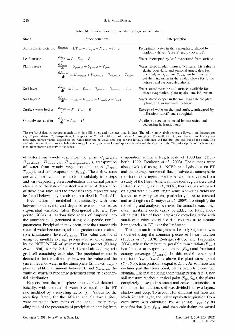
Table AI. Equations used to calculate storage in each stock.

Stock Stock equations Interpretation

Atmospheric moisture dSatmosdt D ETtotal C Pimport � Pexport � Pevent Precipitable water in the atmosphere, altered by

randomly driven ‘events’ and by local ET.

Leaf surface dSleafdt D P � Ecan � F Water intercepted by leaf, evaporated from surface.

Plant tissuesdSgrass

dt D Ugrass,s1 C Ugrass,s2 � Tgrass

dSwoody

dt D Uwoody,s1 C Uwoody,s2 C Uwoody,gw � Twoody

Water stored in plant tissues. Typically, this value iselastic over daily and seasonal timescales. Forthis analysis, Sgrass and Swoody are held constant,but their inclusion in the model allows for futurenutrient and carbon calculations.

Soil layer 1 dSsoil1dt D Isoil1 � Esoil1 � Ugrass,s1 � Uwoody,s1 � Isoil2 Water stored near the soil surface, available for

direct evaporation, plant uptake, and infiltration.

Soil layer 2 dSsoil2dt D Isoil2 � Ugrass,s2 � Uwoody,s2 � Isoil3 Water stored deeper in the soil, available for plant

uptake, and groundwater recharge.

Surface water bodies dSsurfdt D F � Isoil1 � R Storage of water on the land surface, influenced by

infiltration, runoff, and throughfall.

Groundwater aquiferdSgw

dt D Isoil3 � G Aquifer storage, as reflected by increasing anddecreasing hydraulic heads.

The symbol S denotes storage in each stock, in millimetres, and t denotes time, in days. The following symbols represent flows, in millimetres perday: P, precipitation; T, transpiration; E, evaporation; U, root uptake; I, infiltration; F, throughfall; R, runoff; and G, groundwater flow. For a giventime-step, storage values depend on the value from the previous time-step (or the initial conditions) and the flux into and out of the stock. Theanalysis presented here uses a 1-day time-step; however, the model could quickly be adapted for short periods. The subscript ‘max’ indicates themaximum storage capacity of the stock.

of water from woody vegetation and grass (Ugrass,soil1,Uwoody,soil1, Uwoody,soil2, Uwoody,groundwater), transpirationof water from woody vegetation and grass (Tgrass,Twoody), and soil evaporation (Esoil1). These flow ratesare calculated within the model at subdaily time-stepsand vary depending on a combination of external param-eters and on the state of the stock variables. A descriptionof these flow rates and the processes they represent maybe found below; they are also summarized in Table AII.

Precipitation is modelled stochastically, with timebetween both events and depth of events modelled asexponential variables (after Rodrı́guez-Iturbe and Por-porato, 2004). A random time series of ‘imports’ intothe atmosphere is generated using site-specific rainfallparameters. Precipitation may occur once the atmosphericstock of water becomes equal to or greater than the atmo-spheric saturation level, Satmos,sat. This value was foundusing the monthly average precipitable water, estimatedby the NCEP/NCAR 40-year reanalysis project (Kalnayet al., 1996), for the 2Ð5 ð 2Ð5 degree latitude/longitudegrid cell containing each site. The precipitation rate isdeemed to be the difference between this value and thecurrent level of water in the atmosphere (Satmos –Satmos,sat)plus an additional amount between 0 and Satmos,sat, thevalue of which is randomly generated from an exponen-tial distribution.

Exports from the atmosphere are modelled determin-istically, with the rate of water loss equal to the ETrate modified by a recycling factor (fr). Values for therecycling factor, for the African and California sites,were estimated from maps of the ‘annual mean recy-cling ratio of the percentage of precipitation coming from

evaporation within a length scale of 1000 km’ (Tren-berth, 1999; Trenberth et al., 2003). These maps werealso developed using the NCEP reanalysis data on ETand the average horizontal flux of advected atmosphericmoisture over a region. For the Arizona site, values froma study of the North American monsoon region were usedinstead (Dominguez et al., 2008); these values are basedon a grid with a 32-km length scale. Recycling ratios areknown to vary by season, particularly in snow-coveredand arid regions (Dirmeyer et al., 2009). To simplify themodelling and analysis, we used the annual mean; how-ever, variability could easily be added for future mod-elling tests. Use of these large-scale recycling ratios withsmall-scale eddy covariance data requires us to assumehomogeneity in ET over the landscape.

Transpiration from the grass and woody vegetation wasmodelled using the common piecewise linear function(Feddes et al., 1978; Rodrı́guez-Iturbe and Porporato,2004), where the maximum possible transpiration (Emax)is a function of evaporative demand (Epot) and fractionalcanopy coverage (fcanopy). In this model, when soilmoisture (Ssoil1, Ssoil2) is above the plant stress point(SgŁ , SwŁ), transpiration is equal to Emax. As soil moisturedeclines past the stress point, plants begin to close theirstomata, linearly reducing their transpiration rate. Oncesoil moisture reaches a critical point (Sgc, Swc), the plantscompletely close their stomata and cease to transpire. Inthis model formulation, soil was divided into two layers,shallow and deep. To account for different soil moisturelevels in each layer, the water uptake/transpiration fromeach layer was calculated by weighting Emax by itsroot fraction (e.g. fg,s1) and then calculating the actual




Table AII. Equations used to calculate flows to and from each stock.

Water flow Flow equations Interpretation

Totalevapotranspiration

ETtotal D Ecan C Esoil C Tgrass C Twoody The total ET for the model is equal to theevaporation from the leaves and the soilplus the transpiration of the understory andoverstory vegetation.

Evaporation from leafsurface

Ecan D min�Steaf, Epot� Over the course of 1 day, all water presenton leaves evaporates, unless that rate ishigher than the potential ET rate.

Soil evaporation Esoil D{

Epot ð fse, if Ssoil1 ½ Sh

0, if Ssoil1 < Sh

}Soil evaporation is a fraction of the potential

ET.

Grass (understory)uptake

Woody (overstory)uptake

Ugrass,si D Emax,grass�1 � fcanopy�fg,sið

1, if Ssoil i ½ SgŁ,si

�Ssoil i � Sgc,si��SgŁ,si � Sgc,si�

, if Sgc,si < Ssoil i < SgŁ,si

0, if Ssoil i � Sgc,si

Uwoody,si D Emax,woodyfcanopy fw,sið

1, if Ssoil i ½ SwŁ,si�Ssoil i � Swc,si��SwŁ,si � Swc,si�

, if Swc,si < Ssoil i < SwŁ,si

0, if Ssoil i � Swc,si

Transpiration is a piecewise linear functiondynamically dependent on soil moisturestatus (after Rodriquez-Iturbe andPorporato, 2004). The subscripts soil i andsi represents the soil layer; here i D 1 to2. Emax, which represents the averagetranspiration rate under well waterconditions, changes depending on theseason (see text and charts). The fractionsfw,mi and fg,si represent the percentage ofroots present in each soil layer, wherefw,s1 C fw,s2 C fw,g D 1 andfg,s1 C fg,s2 D 1. These values areconstant in this implementation, but couldbe altered to change monthly if enoughdata are available. The fraction fcanopy

indicates the fraction of woody vegetationcanopy coverage.

Uptake fromgroundwater

Uwoody,g D{Emax,woody ð fw,gw, if Ssoil1 � SwŁ,s1 and Ssoil2 � SwŁ,s2

0, otherwise

}The uptake rate of groundwater by woodyvegetation, assumed to be equal to thewell-watered ET, multiplied by the fractionof roots reaching the groundwater table.Uptake is assumed to occur only when thesoil in both layers is below the stress point

Transpiration Tgrass D Ugrass,s1 C Ugrass,s2

Twoody D Uwoody,s1 C Uwoody,s2 C Uwoody,g

Understory transpiration equals the rootwater uptake of the grasses from bothlayers. Overstory transpiration equals theroot water uptake of the woody vegetation,from both soil layers and from thesaturated zone.

Moisture imports andexports

Pimport D fxn[�min, �max, �avg, fxn

(˛min, ˛max, ˛avg

)]Pexport D ETtotal ð �1 � frc�

Import of atmospheric moisture is astochastic function based on the frequency(�) and depth (˛) of rain events observedat the sites. Their occurrence is based on aPoisson arrival process, and their depth israndom and distributed exponentially. Theexport function includes a recycling factor,frc, which states what fraction of theevapotranspired water stays in the system.

Precipitation events Pevent D{Satoms � Satmos,sat � Satmos,sat ð fp, if Satmos > Satmos,sat

0, if Satmos � Satmos,sat

}Precipitation events occur when the totalatmospheric storage of water is above thesaturation point. The amount ofprecipitation can be higher than theamount needed to return to saturation, by afactor of fp. This factor is a random valueranging from 0 to 1, generated by anexponential function.




Table AII. (Continued ).

Water flow Flow equations Interpretation

Infiltration,percolation, andrecharge

Isoil1 D{ min

(Ksoil1, Ssurface,Ssoil1,max � Ssoil1

), if Ssoil1 < Ssoil1,max

0, if Ssoil1 ½ SsoilmaxWater infiltrates from the surface to soil layer

1, percolates from soil layer 1 to 2, andrecharges the groundwater from layer 2.

Isoil2 D{

max(Ksoil1, Ssoil1 � Sfc,s1

),if Sfc,s1 < Ssoil1

0, if Sfc,s1 ½ Ssoil1

0, if Ssoil2 ½ Ssoil2,max

Igw D{

max(Ksoil2, Ssoil2 � Sfc,s2

),if Sfc,s2 < Ssoil2

0,if Sfc,s2 ½ Ssoil2

Runoff R D Ssurf � Isoil1 Runoff is the net difference between theamount that can be stored on the groundsurface and the rate of infiltration into thetop layer of soil.

Throughfall F D{

Pevent � Sleaf,max,if Pevent > Sleaf,max � Sleaf

Pevent, otherwiseThroughfall is the difference between the

amount of rain intercepted and the depthof the precipitation event.

Groundwater G D Sgw � Sgw,max In this model version, G is adjusted so thataquifer storage is constant. However, theframework is adaptable to allow forchanging water table levels.

All flows are measured in depth per time, in the case of the analysis presented here, millimetres per day. When a flow is equal to a storage term, itis implied that this loss occurs over the span of 1 day, so that it is equivalent to a depth/time.

uptake from that layer (Ug,s1) based on the appropriateparameters (SgŁ,soil1, Sgc,soil1, Emax,grass). If vegetationcan reach the underlying saturated zone, the woodyplant uptake from groundwater (Uw,g) is equal to Emax

multiplied by the fraction of roots present in this zone(fw,gw).

Evaporation from the top soil layer was modelled in thesame piecewise linear fashion as transpiration: a fraction(fsc) of Epot, constant when soil moisture is above theplant stomatal closure point and linearly decreasing untilthe soil hygroscopic point (Sh) is reached and evaporationdrops to zero. Additionally, evaporation from the canopysurface on any given day is assumed to be equal to eitherEpot or the amount of water stored on the leaf surfacedue to interception (Sleaf), whichever is lower.

Infiltration into the soil occurs when moisture con-tent in the top layer is lesser than capacity (Ssoil1,max)and a rainfall event occurs. The amount of water infil-trating in 1 day is equal to the remaining soil storagecapacity (Ssoil1,max –Ssoil1) or the conductivity of the soillayer (Ksoil1), whichever is smaller. When soil moistureexceeds field capacity (Sfc,s1, Sfc,s2), infiltration into thelayer below occurs at a daily rate equal to the minimum

of the excess moisture in the leaking layer (Ssoil –Ssoil,fc)and hydraulic conductivity (Ksoil).

Runoff occurs when the rate of water reaching the soil(F) is greater than the infiltration rate into the shallowsoil layer; it can be due to either infiltration excess(Ksoil1 < F) or saturation excess (Ssoil1,max � Ssoil1). Theactual value of F is equal to the precipitation measuredabove the canopy minus canopy and litter interceptionplus stemflow; however, no data on litter interception andstemflow are available for the modelled sites. Instead,we assume that the value of stemflow minus litterinterception is negligible, making F functionally equalto the throughfall rate. The model includes a runoffcoefficient (frun) and a depression storage reservoir (Ssurf)that can be adjusted to account for topographical orother physical factors not otherwise included. Since thecurrent model is not spatially explicit and it is operatedat ecosystem scale, the run-on process was not included.

Finally, the groundwater flow (G) is calculated suchthat groundwater storage remains constant; however, thiscan be adjusted according to the available data or tomeet the desired modelling needs, such as changinggroundwater availability.




understanding ecohydrological connectivity in savannas… · understanding ecohydrological...

Documents