unit 4 marine productivity - cengage · pdf fileth us, scientists ... chlorophyll contained in...

Data Detectives: The Ocean Environment Unit 4 – Marine Productivity

131

Unit 4

Marine ProductivityIn this unit, you will • Discover patterns in global primary productivity.

• Compare terrestrial and marine productivity.

• Explore the key resources required for productivity.

• Correlate variations in marine productivity with limiting resources.

• Investigate sources of marine nutrients.

• Synthesize observations to evaluate the causes of dead zones.

NO

AA

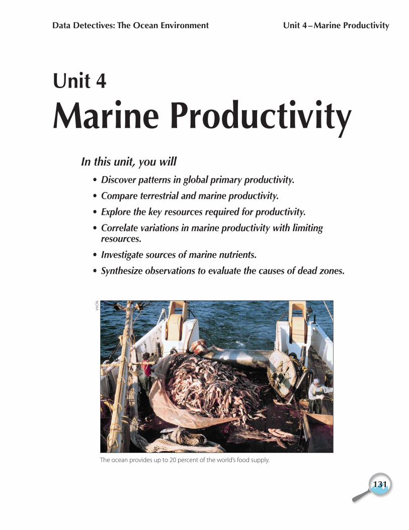
The ocean provides up to 20 percent of the world’s food supply.


132


Bounty from the sea 133

Seafood makes up 20 percent of the world’s food supply, with over one billion people depending on its resources for survival. As seafood harvests have increased over the past two centuries, populations of some species of marine life have decreased and have even become extinct. Given the ocean’s vast area, it is diffi cult to locate, monitor, and track changes in stocks of commercially important fi sh and shellfi sh. Th us, scientists frequently use satellites to indirectly assess the health of fi sheries and the ocean ecosystem.

A key indicator of the ocean’s health is primary productivity, or the rate at which new organic material is produced through photosynthesis (Figure 1 at left ). Photosynthesis is the process by which plant cells containing the green pigment chlorophyll use sunlight to convert water and carbon dioxide into the food (sugars and starches) and oxygen needed by most other organisms. Satellites can measure the amount of chlorophyll contained in single-celled plants in the ocean’s surface layer, from which we can estimate primary productivity.

Food chains (Figure 2) and more complex food webs (Figure 3) illustrate feeding relationships among organisms in biological communities. At the base of food chains and webs are autotrophs, which produce their own food for growth and reproduction through photosynthesis. In the ocean, the primary autotrophs are phytoplankton, microscopic single-celled

Figure 3. A marine food web.

sharksmarine mammals

jellyfish

predatory fish

filter-feeding invertebrates

phytoplankton

filter-feeding fish

baleen whales

zooplankton

seabirds

Bounty from the seaWarm-up 4.1

Autotroph — (“self-feeder”) organism that makes its own food rather than consuming other organisms.

Heterotroph — (“other-feeder”) organism that consumes other organisms.

Figure 2. Simple marine food chain. Arrows represent the transfer of energy from one organism to another through consumption.

marine mammals

fish

zooplankton

phytoplankton

Figure 1. Photosynthesis and respiration.

Photosynthesis by primary producers

Sun

Light

Nutri

ents

Waste heat

Respiration by consumers,

decomposers, and plants

Carbon Dioxide

Water

Organic materials (carbohydrates, etc.)Oxygen


134 Bounty from the sea

plants that drift near the ocean surface. Th e remaining organisms in food webs are heterotrophs, which obtain food by feeding on other organisms.

Th e preservation of each link in a food web is critical for maintaining diverse and healthy biotic communities. However, certain organisms are more critical than others.

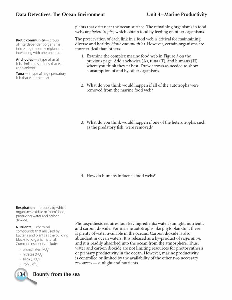
1. Examine the complex marine food web in Figure 3 on the previous page. Add anchovies (A), tuna (T), and humans (H) where you think they fi t best. Draw arrows as needed to show consumption of and by other organisms.

2. What do you think would happen if all of the autotrophs were removed from the marine food web?

3. What do you think would happen if one of the heterotrophs, such as the predatory fi sh, were removed?

4. How do humans infl uence food webs?

Photosynthesis requires four key ingredients: water, sunlight, nutrients, and carbon dioxide. For marine autotrophs like phytoplankton, there is plenty of water available in the oceans. Carbon dioxide is also abundant in ocean waters. It is released as a by-product of respiration, and it is readily absorbed into the ocean from the atmosphere. Th us, water and carbon dioxide are not limiting resources for photosynthesis or primary productivity in the ocean. However, marine productivity is controlled or limited by the availability of the other two necessary resources — sunlight and nutrients.

Nutrients — chemical compounds that are used by bacteria and plants as the building blocks for organic material. Common nutrients include:

• phosphates (PO4

-)

• nitrates (NO3

-)

• silica (SiO4

-)

• iron (Fe3+)

Biotic community — group of interdependent organisms inhabiting the same region and interacting with one another.

Respiration — process by which organisms oxidize or “burn” food, producing water and carbon dioxide.

Anchovies — a type of small fi sh, similar to sardines, that eat zooplankton.

Tuna — a type of large predatory fi sh that eat other fi sh.


Bounty from the sea 135

5. How do you think the availability of limiting resources might vary in the ocean? (Where or when would they be high or low?)

6. Considering the availability of limiting resources, where would you expect phytoplankton to be most productive or least productive? (Near the equator or near the poles? Near the coast or in the open ocean?)

7. How is the productivity of autotrophs important to society? Describe three diff erent ways in which a severe decrease in primary productivity would aff ect society.

a.

b.

c.


136 Bounty from the sea


The life-giving ocean 137

Phytoplankton are tiny — several of them could fi t side-by-side across the width of a human hair — but collectively, they pack a wallop. Phytoplankton are primary producers, serving as the fi rst link in almost every food chain in the ocean. Th ey transform water and carbon dioxide into carbohydrates, which they use for producing energy for growth and reproduction. Phytoplankton, in turn, are food for other organisms, passing carbohydrates and other nutrients up the food chain. Because phytoplankton release oxygen during photosynthesis, they also play a signifi cant role in maintaining the proper balance of Earth’s atmospheric gases. Phytoplankton produce about half of the world’s oxygen and, in doing so, remove large amounts of carbon dioxide from the atmosphere.

Given the central role of phytoplankton in stabilizing the mixture of gases in Earth’s atmosphere and in providing food for other organisms, it is important to monitor their location and rate of productivity. Although it is impossible to directly measure the productivity of phytoplankton on a global scale, there are several ways of making indirect calculations. One method relies on the distinctive way that chlorophyll, the green pigment in phytoplankton and other plants, refl ects sunlight. By using satellites to measure the chlorophyll concentration of the ocean surface layer, scientists can estimate the rate at which phytoplankton produce carbohydrates (Figure 1). Because carbon is the key element in the process, productivity is measured in terms of kilograms of carbon converted per square meter of ocean surface (kgC/m2) per year.

Global primary productivityIn this exercise you will examine global primary productivity and its relation to the factors that support phytoplankton growth.

Launch ArcMap, and locate and open the ddoe_unit_4.mxd fi le.

Refer to the tear-out Quick Reference Sheet located in the Introduction to this module for GIS defi nitions and instructions on how to perform tasks.

In the Table of Contents, right-click the Primary Productivity data frame and choose Activate.

Expand the Primary Productivity data frame.

Th is data frame shows the average annual primary productivity for terrestrial and marine environments. During their respective winters, regions near the north and south poles receive little or no sunlight, making satellite measurements impossible. Nonetheless it is reasonable to assume that, with no sunlight during winter, there is relatively little primary productivity in these regions .

The life-giving oceanInvestigation 4.2

Primary productivity — the rate at which new organic material is formed by photosynthesis.

PhotosynthesisThe general chemical equation for photosynthesis is:

carbondioxide

water glucose(carbohydrate)

oxygen

sunlight

6 CO2 + 6 H

2O C

6H

12O

6 + 6 O

2

Figure 1. The MODIS (MODerate-resolution Imaging Spectrometer) instrument on the Terra satellite is the latest tool for measuring primary productivity from space.

NA

SA


138 The life-giving ocean

1. What colors represent areas of highest and lowest productivity?

a. Highest.

b. Lowest.

2. On Map 1, circle the land areas with the highest productivity using solid lines, and the land areas with the lowest productivity using dashed lines.

Map 1 — Areas of highest and lowest productivity

Turn off the Terrestrial Productivity layer.

Using the Zoom In tool , examine, in detail, the areas with the highest marine productivity.

When you are fi nished, click the Full Extent button to zoom back out to view the entire map.

3. Mark the ocean areas with highest productivity on Map 1 using the label H (high), and the ocean areas of lowest productivity using the label L (low).

4. Where is marine productivity generally

a. highest?

b. lowest?



5. Compare the locations of regions of high terrestrial and marine productivity on Map 1. Describe any geographic patterns or similarities in their distribution.

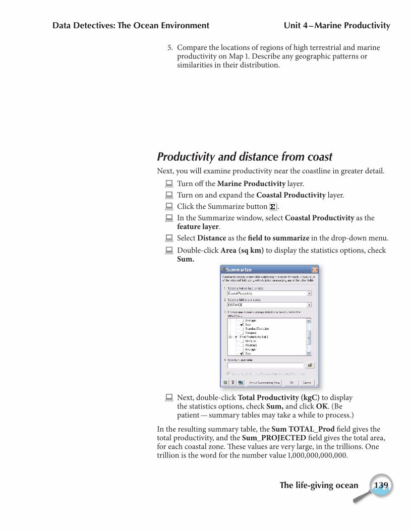
Productivity and distance from coastNext, you will examine productivity near the coastline in greater detail.

Turn off the Marine Productivity layer.

Turn on and expand the Coastal Productivity layer.

Click the Summarize button .

In the Summarize window, select Coastal Productivity as the feature layer.

Select Distance as the fi eld to summarize in the drop-down menu.

Double-click Area (sq km) to display the statistics options, check Sum.

Next, double-click Total Productivity (kgC) to display the statistics options, check Sum, and click OK. (Be patient — summary tables may take a while to process.)

In the resulting summary table, the Sum TOTAL_Prod fi eld gives the total productivity, and the Sum_PROJECTED fi eld gives the total area, for each coastal zone. Th ese values are very large, in the trillions. One trillion is the word for the number value 1,000,000,000,000.



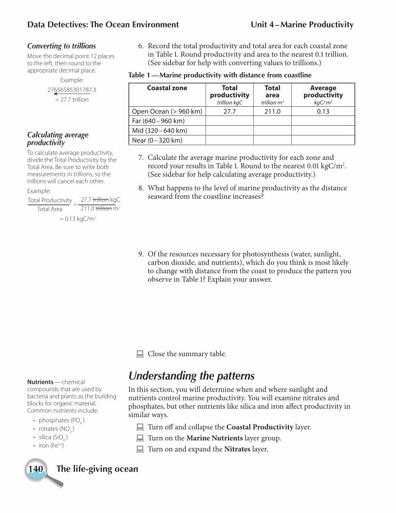
6. Record the total productivity and total area for each coastal zone in Table 1. Round productivity and area to the nearest 0.1 trillion. (See sidebar for help with converting values to trillions.)

Table 1 — Marine productivity with distance from coastline

Coastal zone Total productivity

trillion kgC

Total area

trillion m2

Average productivity

kgC/ m2

Open Ocean (> 960 km) 27.7 211.0 0.13

Far (640 – 960 km)

Mid (320 – 640 km)

Near (0 – 320 km)

7. Calculate the average marine productivity for each zone and record your results in Table 1. Round to the nearest 0.01 kgC/m2. (See sidebar for help calculating average productivity.)

8. What happens to the level of marine productivity as the distance seaward from the coastline increases?

9. Of the resources necessary for photosynthesis (water, sunlight, carbon dioxide, and nutrients), which do you think is most likely to change with distance from the coast to produce the pattern you observe in Table 1? Explain your answer.

Close the summary table.

Understanding the patternsIn this section, you will determine when and where sunlight and nutrients control marine productivity. You will examine nitrates and phosphates, but other nutrients like silica and iron aff ect productivity in similar ways.

Turn off and collapse the Coastal Productivity layer.

Turn on the Marine Nutrients layer group.

Turn on and expand the Nitrates layer.

Nutrients — chemical compounds that are used by bacteria and plants as the building blocks for organic material. Common nutrients include:

• phosphates (PO4

-)

• nitrates (NO3

-)

• silica (SiO4

-)

• iron (Fe3+)

Converting to trillionsMove the decimal point 12 places to the left, then round to the appropriate decimal place.

Example:

27656585301787.3

= 27.7 trillion

Calculating average productivityTo calculate average productivity, divide the Total Productivity by the Total Area. Be sure to write both measurements in trillions, so the trillions will cancel each other.

Example:

= 0.13 kgC/m2

Total Productivity

Total Area

27.7 trillion kgC

211.0 trillion m2=



Latitude bandsLow latitudes

0° – 30° N and Snear equator

Middle latitudes

30° – 60° N and Sbetween equator and poles

High latitudes

60° – 90° N and Snear poles

Nitrates and phosphates are important nutrients that are used by autotrophs for building complex molecules needed for growth and development. Th e Nitrates layer displays the average annual level of nitrates in the world’s oceans in terms of micromolarity, or millionths of a mole of nitrate per liter of seawater (see sidebar).

10. Which latitude bands have the highest and lowest concentrations of nitrates? (See Latitude bands sidebar for help.)

a. Highest.

b. Lowest.

Turn off and collapse the Nitrates layer.

Turn on and expand the Phosphates layer.

Th e Phosphates layer shows the average annual concentration of phosphates in the world’s oceans in terms of micromolarity.

11. Which latitude bands have the highest and lowest concentration of phosphates?

a. Highest.

b. Lowest.

12. Are the patterns for both nutrients similar? If not, how do they diff er?

Turn off and collapse the Phosphates layer.

Turn on the Solar Radiation Flux layer.

Th is layer shows the average annual solar radiation that strikes Earth’s surface, in watts per square meter (W/sq m).

Click the Media Viewer button and open the Solar Flux Movie.

Th is animation shows changes in solar radiation throughout the year. Th e time of year and the legend appear at the bottom of the image.

View the movie several times.

MicromolesMicromolarity is a measure of concentration used to describe very weak solutions. The metric prefi x micro represents one millionth. A mole is 6.02 × 1023 molecules (or atoms), so a micromole is one millionth of a mole, or 6.02 × 1017 molecules. That seems like a lot, but when dissolved in a liter of water (55.5 moles, or about 3.34 × 1025 water molecules) it’s only one molecule of nutrient for every 200 million water molecules. That’s a weak solution.



Use the Solar Radiation Flux layer and the Solar Flux Movie to answer the following questions.

13. Near what latitude is the average solar radiation throughout the entire year

a. highest?

b. lowest?

14. How does the pattern of nutrient concentration you noted in questions 10 and 11 compare to the pattern of solar radiation? Explain your answer.

Close the Media Viewer window.

Click the Media Viewer button , and open the Productivity Movie.

Th is animation shows marine productivity throughout the year. Th e time of year is indicated at the top of the image, and the legend appears at the bottom. Black areas at high latitudes are where there was no sunlight during the winter; you may assume these areas have relatively little productivity.

Study the movie to examine how productivity changes throughout the year. Focus on only the extreme high and low levels of productivity. You will need to play the movie several times to fi ll in Table 2.

15. In Table 2, enter the months and season when productivity is highest and lowest in each hemisphere. (See sidebar for help with the seasons.)

Table 2 — Productivity extremes by hemisphere

Hemisphere Months of high productivity

Season Months of low productivity

Season

Northern

Southern

Close the Media Viewer window.

Earth’s Seasons are • Caused by the tilt of Earth’s

axis.

• Opposite in the Northern and Southern Hemispheres.

Dates(typical)

Hemisphere

N S

Dec 21 –

Mar 20Winter Summer

Mar 20 –

Jun 21Spring Fall

Jun 21 –

Sep 22Summer Winter

Sep 22 –

Dec 21Fall Spring



Th ere is very little seasonal variability in nutrients in the high-latitude oceans because the thermocline, or temperature gradient between shallow and deep water, is small, due to low solar-radiation input. Th is allows free circulation between deep nutrient-rich water and shallow nutrient-poor water. Th e year-round strong solar radiation in equatorial regions creates a strong thermocline (warm shallow water and cold deep water), which inhibits shallow- and deep-water circulation. Equatorial upwelling does bring nutrients to the surface in some areas, but nutrient levels are generally low at low latitudes, particularly during the summer when the air is very stable and winds are weak.

16. Discuss the infl uence that each of the following factors has on productivity at high latitudes, and how productivity in high-latitude regions may change with the seasons.

a. Sunlight.

b. Nutrients.

17. Discuss how sunlight and nutrient levels contribute to the productivity pattern at low latitudes, and how productivity in that region may change with the seasons.

a. Sunlight

b. Nutrients



In the next activity, you will learn more about marine productivity, the sources of marine nutrients, and the processes that bring nutrients to the surface near the coastlines and in the open ocean.

Quit ArcMap and do not save changes.


Resources for productivity 145

Mean, green food-making machinesWith few exceptions, life on Earth depends on photosynthesis, the biological process that converts solar energy and inorganic compounds into food. Only autotrophs or “producers,” including green plants and phytoplankton, are capable of photosynthesis. Th ey contain the pigment chlorophyll, which uses solar energy to convert carbon dioxide and water into carbohydrates (Figure 1). Th e amount of carbon converted to food by autotrophs is referred to as primary productivity. Autotrophs use some of this food immediately, and store the remainder for later use, to be converted back to energy through the process of respiration. Phytoplankton are consumed by other organisms which are, in turn, consumed by other organisms up the food chain. Collectively, these consumer organisms are called heterotrophs.

Exceptions to the ruleGreen plants and phytoplankton are not the only organisms capable of synthesizing their own food. In the last 40 years, scientists have discovered biological communities that are not based on the sun’s energy. Th e autotrophs in these communities are microbes that convert carbon dioxide and water into food using chemicals rather than sunlight. Th is process is called chemosynthesis (Figure 2). Chemosynthetic bacteria thrive in the high temperatures and pressures of environments like deep-sea volcanic vents. Th ey synthesize food using the chemical energy of sulfur compounds emerging from the vents. Chemosynthesis supports a diverse community of organisms (Figure 3).

Food for thought—bottoms up!Food webs illustrate the feeding relationships among organisms in a biotic community. Th e arrows represent the transfer of energy from one organism to another through consumption (Figure 4). Autotrophs produce most of Earth’s atmospheric oxygen as a by-product of photosynthesis, and are

Resources for productivityReading 4.3

Figure 2. Process of chemosynthesis.

carbon dioxide (COcarbon dioxide (CO2 2

))+ water (H+ water (H

22O)O)

+ hydrogen sulfide (H+ hydrogen sulfide (H22S)S)

+ oxygen (O+ oxygen (O2 2

))==

carbohydrate (CHcarbohydrate (CH22O)O)

+ sulfuric acid (H+ sulfuric acid (H22SOSO

4 4 ))

NO

AA

Figure 3. Tube worms at hydrothermal vents consume chemosynthetic bacteria.

NO

AA

Figure 4. Marine food web.

sharksmarine mammals

jellyfish

predatory fish

filter-feeding invertebrates

phytoplankton

filter-feeding fish

baleen whales

zooplankton

seabirds

Figure 1. Photosynthesis and respiration.

Photosynthesis by primary producers

Sun

Light

Nutri

ents

Waste heat

Respiration by consumers,

decomposers, and plants

Carbon Dioxide

Water

Organic materials (carbohydrates, etc.)Oxygen


146 Resources for productivity

the foundation of nearly all terrestrial and aquatic food chains. Th us, primary productivity in terrestrial and marine environments is a key indicator of the overall health of the environment. Our ability to monitor primary productivity has profound economic and environmental importance.

1. Compare and contrast the two processes that autotrophs use to synthesize food.

2. What does the number of arrows leading from one organism to others suggest about that organism’s importance in the food web?

3. What does the number of arrows leading to an organism suggest about that organism’s likelihood of becoming endangered or extinct?

Resources for photosynthesisPrimary productivity levels vary with season and geographic location. You have identifi ed and examined regions of extremely high and low productivity on land and in the ocean. Th ese patterns of productivity are dictated by the availability of the resources necessary for photosynthesis. Autotrophs require carbon dioxide, water, sunlight, and nutrients to photosynthesize (Figure 1 on the previous page). When these resources are not present in adequate amounts for photosynthesis, they are referred to as limiting factors. Below, you will examine the likelihood of each resource being a limiting factor in productivity.

Carbon dioxideCarbon dioxide is not likely to be a limiting factor in terrestrial or marine photosynthesis because it is plentiful in the atmosphere, as a result of respiration and human activities. As organisms convert food into energy, they release carbon dioxide (Figure 1). When humans burn fossil fuels like petroleum, coal, and natural gas, huge quantities of carbon dioxide are released into the atmosphere. Carbon dioxide is readily absorbed into the ocean from the atmosphere, so it is in good supply there as well.



WaterWater is oft en a limiting factor for productivity in terrestrial environments. Productivity in deserts is very low because deserts lack the water needed to sustain many plants. In the ocean, water is never a limiting factor.

SunlightIn the context of productivity, the sun’s most important role is providing the light energy that drives photosynthesis. Th e availability of light to autotrophs varies, depending on latitude, season, and time of day. Th erefore, there are places and times where sunlight is a limiting factor.

NutrientsAutotrophs use inorganic compounds containing nitrogen, phosphorus, potassium, calcium, silicon, and iron to build organic molecules. Th e concentrations of these nutrients vary throughout the environment. Nitrogen and phosphorus are particularly important because they are required in large quantities and play a critical role in growth and reproduction. Inorganic forms of nitrogen are the building blocks for amino acids, proteins, and genetic material (DNA, RNA). Similarly, phosphorus is an essential component of energy transport molecules (ATP), genetic material, and structural materials (bone, teeth, shell).

Despite the abundance of nitrogen gas in the atmosphere, it is oft en a limiting resource because it can be utilized by autotrophs only in certain forms. In the nitrogen cycle, nitrogen gas is converted to its most useful form, nitrate, through a series of reactions carried out by bacteria and fungi in the soil (Figure 5). Nitrates may be utilized by land plants, or may be carried to the ocean in groundwater or runoff and used by phytoplankton.

Unlike nitrogen, phosphorus never exists as a gas. Phosphorus originates in rocks in Earth’s crust in the form of phosphate salts, which are liberated from rocks by weathering (Figure 6 on the following page). Phosphates are also an ingredient in some detergents and fertilizers. Precipitation carries phosphates into the soil, and runoff and ground water transport them to the ocean.

Organic or inorganic?The terms organic and inorganic originally came from the idea that chemical compounds could be divided into two categories: those coming from or composed of plants or animals (organic), and those extracted from minerals and ores (inorganic).

Chemists now think of organic compounds as those that contain carbon. This defi nition works well for many compounds, but there are exceptions. For example, carbon dioxide is a carbon-based compound, but it is not considered organic.

Figure 5. The nitrogen cycle.

Ammonium, nitrates, and nitrites in soil

and rock.

Decomposition

Bacteria

Decomposition

Organisms Organisms

Bacteria

BacteriaBacteriaBacteria

Plant and animal wastes

Plant and animal wastes

Ammonium, nitrates, and

nitrites dissolved in seawater.

River transport

Dissolved N2

N2

ATMOSPHERE

OCEANLAND Nitrogen in sediments



4. Various human activities contribute additional nutrients to the ocean ecosystem. How might these additions infl uence marine productivity?

Sources of nutrientsMost of the nutrients utilized by phytoplankton in surface waters originate on land. Nitrates and phosphates in the soil dissolve easily in water. Th ese nutrients are easily leached or removed from the soil by precipitation and runoff , and are carried by groundwater, streams, and rivers to the ocean. Near the coasts, phytoplankton thrive on the nutrients entering the ocean from land, resulting in high productivity. However, large portions of the nutrients entering the ocean are not utilized and eventually sink to the ocean fl oor, accumulating in the sediment.

Not all nutrients enter the ocean from land. When marine plants and animals die they sink to the bottom, where decomposition liberates the nutrients, making them available for use again. However, except in shallow waters over the continental shelf, the nutrients on the ocean bottom can be utilized only when they are brought from the depths to the surface via upwelling, the upward movement of deep, cold bottom water to the surface. Coastal upwelling occurs in nearshore environments where strong winds blow parallel to the shore (Figure 7). Ekman transport causes the surface currents to defl ect away from the shore, which pulls deep, cold, nutrient-rich water toward the surface. As you learned in Investigation 2.2 and Reading 2.3, Ekman transport is an off set between a current direction and its associated wind. In the Northern Hemisphere Ekman transport is defl ected to the right, and in the Southern Hemisphere Ekman transport is defl ected to the left . Th is phenomenon is caused by the Coriolis eff ect and by the slowing and defl ection of water due to friction among successively deeper layers of water.

Figure 6. The phosphorus cycle.

Organisms

Upwelling

Dissolved phosphates

River transport to

oceans

Phosphorus in soil

Phosphorus in organisms

Phosphorus in sediments

Phosphorus in crustal rocks

Weathering, soil formationMining &

AgricultureMinor onshore transport of phosphates by seabirds, fishing

Phosphorus returned to biosphere via uplift

or volcanism

Figure 7. Coastal upwelling.

Wind parallel to shore

Water moving offshore due to Ekman transport



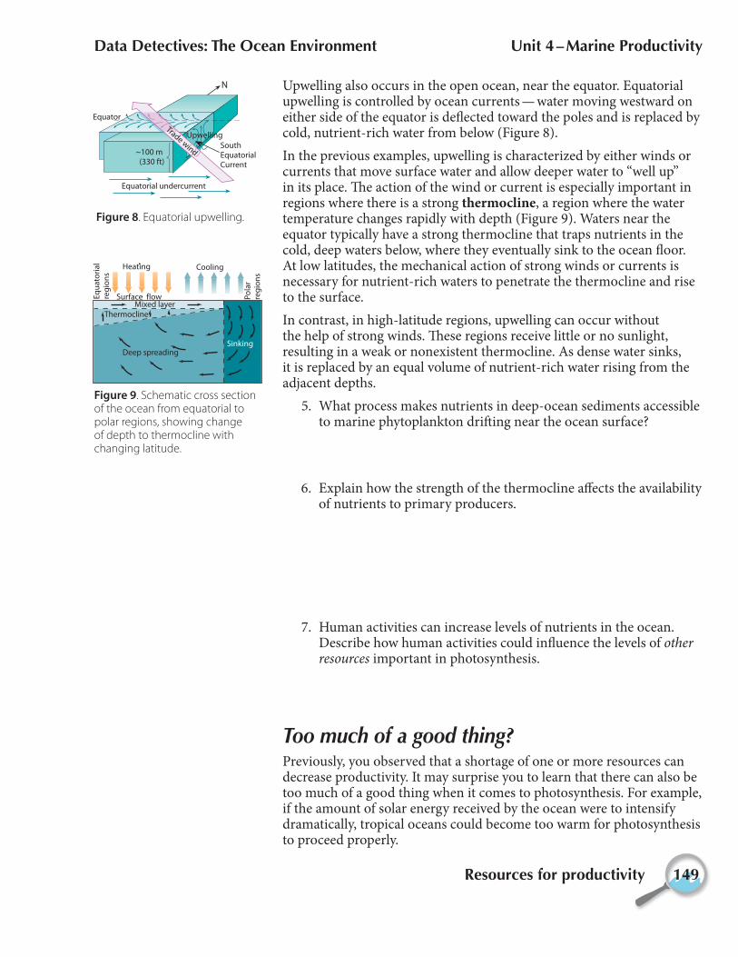
Upwelling also occurs in the open ocean, near the equator. Equatorial upwelling is controlled by ocean currents — water moving westward on either side of the equator is defl ected toward the poles and is replaced by cold, nutrient-rich water from below (Figure 8).

In the previous examples, upwelling is characterized by either winds or currents that move surface water and allow deeper water to “well up” in its place. Th e action of the wind or current is especially important in regions where there is a strong thermocline, a region where the water temperature changes rapidly with depth (Figure 9). Waters near the equator typically have a strong thermocline that traps nutrients in the cold, deep waters below, where they eventually sink to the ocean fl oor. At low latitudes, the mechanical action of strong winds or currents is necessary for nutrient-rich waters to penetrate the thermocline and rise to the surface.

In contrast, in high-latitude regions, upwelling can occur without the help of strong winds. Th ese regions receive little or no sunlight, resulting in a weak or nonexistent thermocline. As dense water sinks, it is replaced by an equal volume of nutrient-rich water rising from the adjacent depths.

5. What process makes nutrients in deep-ocean sediments accessible to marine phytoplankton drift ing near the ocean surface?

6. Explain how the strength of the thermocline aff ects the availability of nutrients to primary producers.

7. Human activities can increase levels of nutrients in the ocean. Describe how human activities could infl uence the levels of other resources important in photosynthesis.

Too much of a good thing?Previously, you observed that a shortage of one or more resources can decrease productivity. It may surprise you to learn that there can also be too much of a good thing when it comes to photosynthesis. For example, if the amount of solar energy received by the ocean were to intensify dramatically, tropical oceans could become too warm for photosynthesis to proceed properly.

Figure 8. Equatorial upwelling.

Equatorial undercurrent

Trade wind

Equator

N

Upwelling

South Equatorial Current

~100 m (330 ft)

Figure 9. Schematic cross section of the ocean from equatorial to polar regions, showing change of depth to thermocline with changing latitude.

Mixed layerSurface flow

Heating Cooling

Eq

ua

tori

al

reg

ion

s

Sinking

Thermocline

Po

lar

reg

ion

s

Deep spreading



Similarly, nutrients can be present in quantities so high that they become harmful. High levels of nutrients in coastal waters may cause a sharp increase in phytoplankton, which reduces light penetration, clogs the gills of marine organisms, and pollutes the water with waste products, some of which are toxic to other marine life. Th is may lead to hypoxia, a dramatic decrease in dissolved oxygen, or even anoxia, a total absence of dissolved oxygen, which can drive away mobile organisms and kill sedentary organisms.

Two conditions contribute to hypoxia in subsurface waters.

• Stratifi cation, or layering of the water column. Nutrient-laden runoff fl owing into the ocean is less dense than salt water and fl oats on the surface. In summer, warm weather and calm seas inhibit mixing of the shallow, warm water with deeper, colder water. As a result, the oxygen from photosynthesis remains at the surface.

• Increased decomposition at depth, due to higher surface productivity. Phytoplankton die or are eaten by other organisms, creating large amounts of organic waste that sinks to the ocean fl oor. As the waste decomposes, nutrients are recycled but oxygen is also consumed, creating hypoxic conditions.

Th e Gulf of Mexico is an important U.S. commercial fi shery. In 2002, the Gulf accounted for 16.9 percent by weight (771,000 metric tons [850,000 U.S. tons]) and 24.7 percent by dollar value ($693 million) of the entire U.S. fi sh and shellfi sh catch. Each summer, a large hypoxic region known as the Mississippi River dead zone forms off the coast of Louisiana (Figure 10). Th e lack of dissolved oxygen in this region causes both the quantity and the diversity of economically important marine life to decrease dramatically, with potentially dire economic consequences.

8. Describe how an increase in nutrient levels can actually lower marine productivity in the marine ecosystem.

9. Name two human activities that could result in an overabundance of nutrients being delivered to coastal waters. Explain your answer.

Figure 10. Location and extent of the 1993 Mississippi River dead zone.

Louisiana

Gulf of Mexico

Texas

Mississippi

Deadzone

Sedentary organisms — organisms that are attached to a surface and cannot move freely.

Is the Mississippi River dead zone unique?In the U.S. alone, more than half of the estuaries experience hypoxia during the summer; up to a third experience anoxia.



10. How might reduced light penetration aff ect primary producers as well as other animals higher up the food chain?

In the next investigation, you will examine changes in the Mississippi River dead zone from 1986 to 1993, and investigate patterns in the distribution of dead zones around the world.


Dead zones 153

Dead zonesInvestigation 4.4

Th ere are parts of the ocean where no fi sh swim, and where the bottom may be littered with the remains of bottom-dwelling crabs, clams, and worms. Th ese areas, known as dead zones, pose a growing environmental concern. Th e causes of dead zones are complex and involve pollution in the form of excess nutrients from agriculture, industry, urbanization, and other sources.

Creating a dead zoneOne of the largest dead zones in the world occurs in the northern Gulf of Mexico, where the Mississippi River fl ows into the open ocean off the coast of Louisiana. Starting in the 1950s, the waters of the Mississippi River began to show signs of elevated nutrient levels, particularly nitrogen compounds from agricultural runoff in the Mississippi River basin. At the same time, a dead zone began to form adjacent to the Mississippi delta in the Gulf of Mexico.

In this investigation, you will look at the size of the Mississippi River dead zone over time, and compare it to dead zones on the east coast of the U.S. and around the world. Th is will help you to better understand how and where dead zones form, and to predict where they may develop in the future.



In the Table of Contents, right-click the Mississippi River Dead Zone data frame and choose Activate.

Expand the Mississippi River Dead Zone data frame.

The Mississippi River dead zoneTh is data frame shows the Mississippi River and the Mississippi River watershed. Th e 31 states that are either partially or completely within the Mississippi River watershed boundary are shown in gray.

Th e Mississippi River watershed covers are large part of the 48 contiguous states, and many activities aff ect the quality of the water before it empties into the Gulf of Mexico. Next, you will examine how water is used, to identify possible sources of the excess nutrients in the Mississippi River dead zone.

Turn on the Water Consumption layer.

Watershed — the total area of land drained by a river and its tributaries.


154 Dead zones

Th is layer consists of pie charts for the 48 contiguous states, each showing the percentage of water consumed by six major water-use sectors (see sidebar). Th e overall size of each pie represents the total amount of water consumed by that state, and the slices represent the percentage of water used by each water-use sector.

1. Which activities are the primary consumers of water in states within the Mississippi River watershed?

a. Eastern portion of the watershed.

b. Western portion of the watershed.

2. How might these activities contribute to nutrient enrichment of the Mississippi River?

Turn off and collapse the Water Consumption layer.

Turn on the Precipitation layer.

Th is layer shows average precipitation, in centimeters per year. Areas with low precipitation are shown in yellow and brown, and areas with high precipitation in blue.

3. Where is precipitation in the Mississippi River watershed

a. highest?

b. lowest?

Runoff from the land is one mechanism for transporting nutrients from farms and fi elds to the river.

Water-use sectors • Commercial — facilities and

institutions including hotels, restaurants, hospitals, and schools.

• Domestic — household use.

• Industrial — producing steel, chemicals, paper, plastics, minerals, petroleum, and other products.

• Power — steam-driven electric generators. (Does not include hydroelectric power.)

• Mining — extracting minerals, oil, and natural gas.

• Agriculture — raising animals and irrigating crops.


Dead zones 155

4. Study the precipitation patterns, then predict where you would expect runoff to be highest in the Mississippi River watershed.

Turn off the Precipitation layer.

Turn on the Runoff layer.

Th is layer shows average runoff within the Mississippi River watershed, in centimeters per year. Dark blue represents high runoff and light blue represents low runoff .

5. Which part of the Mississippi River watershed has the highest annual runoff ?

6. Describe any relationships you observe between the precipitation and the runoff patterns.

7. How might levels of precipitation and runoff infl uence the size of the Mississippi River dead zone?

Turn off the Runoff and Mississippi River System layers.

Development of the Mississippi River dead zoneIn this section, you will look at the extent of the dead zone during four diff erent time periods, and compare the size of the dead zone to the climate data for the Mississippi River watershed during those four periods.

Click the QuickLoad button .

Select Spatial Bookmarks, choose Gulf of Mexico, and click OK.

In 1985, scientists began sampling water off the Louisiana coast to monitor the extent and characteristics of the Mississippi River dead zone.

Turn on the Mississippi River Dead Zone layer group.

Turn on the 1986 Dead Zone layer.

Click the Identify tool .


156 Dead zones

In the Identify Results window, select the 1986 Dead Zone layer from the list of layers.

Click inside the dead-zone to display the area of the dead zone for that year.

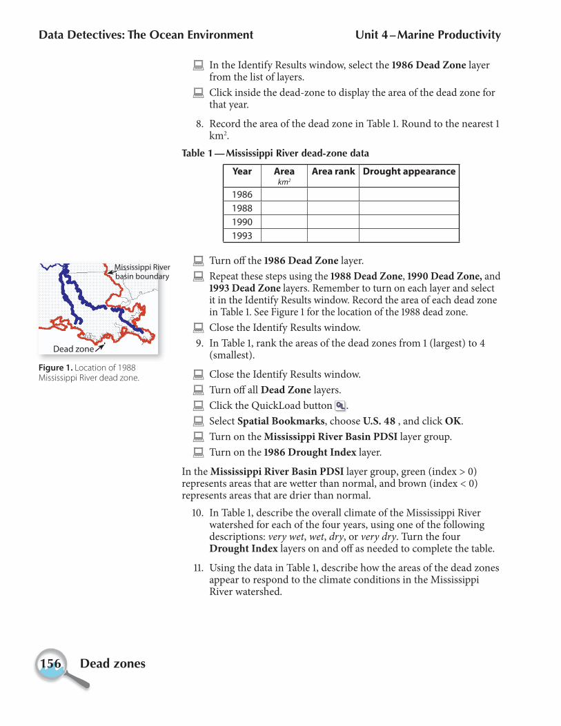
8. Record the area of the dead zone in Table 1. Round to the nearest 1 km2.

Table 1 — Mississippi River dead-zone data

Year Area km2

Area rank Drought appearance

1986

1988

1990

1993

Turn off the 1986 Dead Zone layer.

Repeat these steps using the 1988 Dead Zone, 1990 Dead Zone, and 1993 Dead Zone layers. Remember to turn on each layer and select it in the Identify Results window. Record the area of each dead zone in Table 1. See Figure 1 for the location of the 1988 dead zone.

Close the Identify Results window.

9. In Table 1, rank the areas of the dead zones from 1 (largest) to 4 (smallest).


Turn off all Dead Zone layers.

Click the QuickLoad button .

Select Spatial Bookmarks, choose U.S. 48 , and click OK.

Turn on the Mississippi River Basin PDSI layer group.

Turn on the 1986 Drought Index layer.

In the Mississippi River Basin PDSI layer group, green (index > 0) represents areas that are wetter than normal, and brown (index < 0) represents areas that are drier than normal.

10. In Table 1, describe the overall climate of the Mississippi River watershed for each of the four years, using one of the following descriptions: very wet, wet, dry, or very dry. Turn the four Drought Index layers on and off as needed to complete the table.

11. Using the data in Table 1, describe how the areas of the dead zones appear to respond to the climate conditions in the Mississippi River watershed.

Figure 1. Location of 1988 Mississippi River dead zone.

Dead zone

Mississippi River basin boundary


Dead zones 157

12. Explain the changes in the area of the dead zone in terms of runoff and nutrients in the Gulf of Mexico.

Th e Mississippi River dead zone is not the only one in the U.S. or the world. Next, you will examine potential factors that may contribute to the formation of other dead zones.

Global dead zones Click the QuickLoad button .

Select Data Frames, choose Global Dead Zones, and click OK.

Th e Global Dead Zones data frame shows the locations of dead zones throughout the world.

13. Describe the locations of the two primary clusters of dead zones.

Dead zones and populationSome scientists have noted that dead zones are related to the density of human populations of the adjacent continents. Many believe that dead zones may become the most signifi cant human impact on oceans and ocean ecosystems in the 21st century. In this section, you will investigate this idea and the ways in which increasing populations infl uence the size and number of dead zones.

14. If dead zones are related to areas with high population density, where on the map would you expect to fi nd areas with high population density?

You can test your prediction by looking at the global population distribution, and see how it relates to the current distribution of dead zones.

Turn on the Global Population layer.

Th e Global Population layer shows the population for 1°× 1° cells (approximately rectangular regions within a grid) over Earth’s surface.

How large an area is a 1° x 1° cell?The spacing between latitude lines is fairly constant, but the spacing between longitude lines decreases with distance from the equator. Thus, the areas of 1° x 1° cells get smaller with increasing distance from the equator.

At the equator, a 1° x 1° cell has an area of about 12,500 km2. At 60° latitude, the area of a 1° x 1° cell is only half that size, about 6200 km2.


158 Dead zones

15. Some scientists argue that high population density cause dead zones. Examine the global patterns of population density and dead zones. Describe any observations that

a. support (provide evidence in favor of) the idea that high population density causes dead zones.

b. refute (provide evidence against) the idea that high population density causes dead zones.

Th ere appears to be a connection between high population density and the formation of dead zones, but it is not a clear or consistent relationship. One possibility is that there is some important diff erence (other than size) between the populations adjacent to the regions where dead zones form and those near regions where dead zones do not form. Next, you will explore the possibility that economic diff erences among populations are a factor in the formation of dead zones.

Turn off the Global Population layer.

Turn on the Gross Domestic Product layer.

Gross Domestic Product (GDP) is the total value of goods and services produced by a nation within that nation’s boundaries. Indirectly, it is a measure of the resources (energy, raw materials, people) available to and utilized by that nation.

Now you will determine the average GDP of countries adjacent to dead zones and compare it to the average GDP of countries without dead zones.

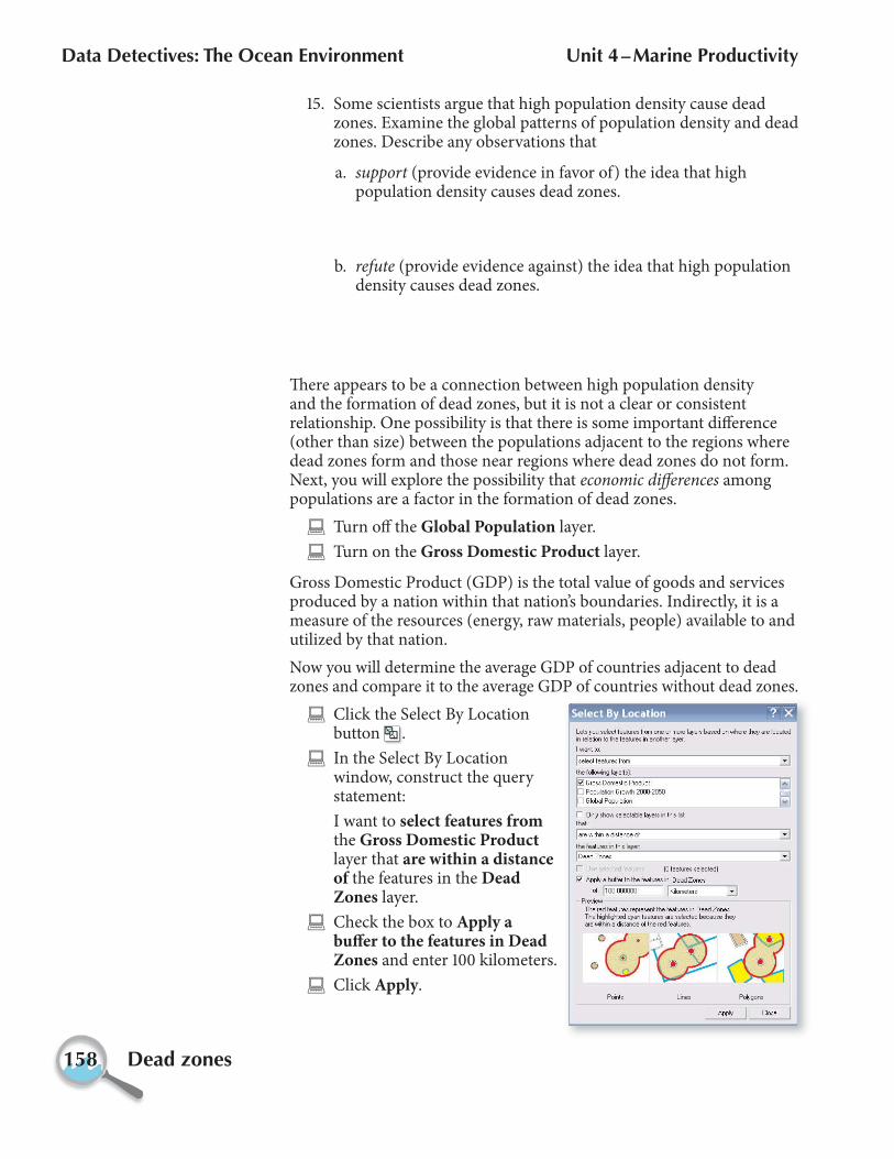
Click the Select By Location button .

In the Select By Location window, construct the query statement:

I want to select features from the Gross Domestic Product layer that are within a distance of the features in the Dead Zones layer.

Check the box to Apply a buff er to the features in Dead Zones and enter 100 kilometers.

Click Apply.


Dead zones 159

Close the Select By Location window.

Th e countries that are near dead zones will be outlined. Next you will calculate statistics on the selected data.

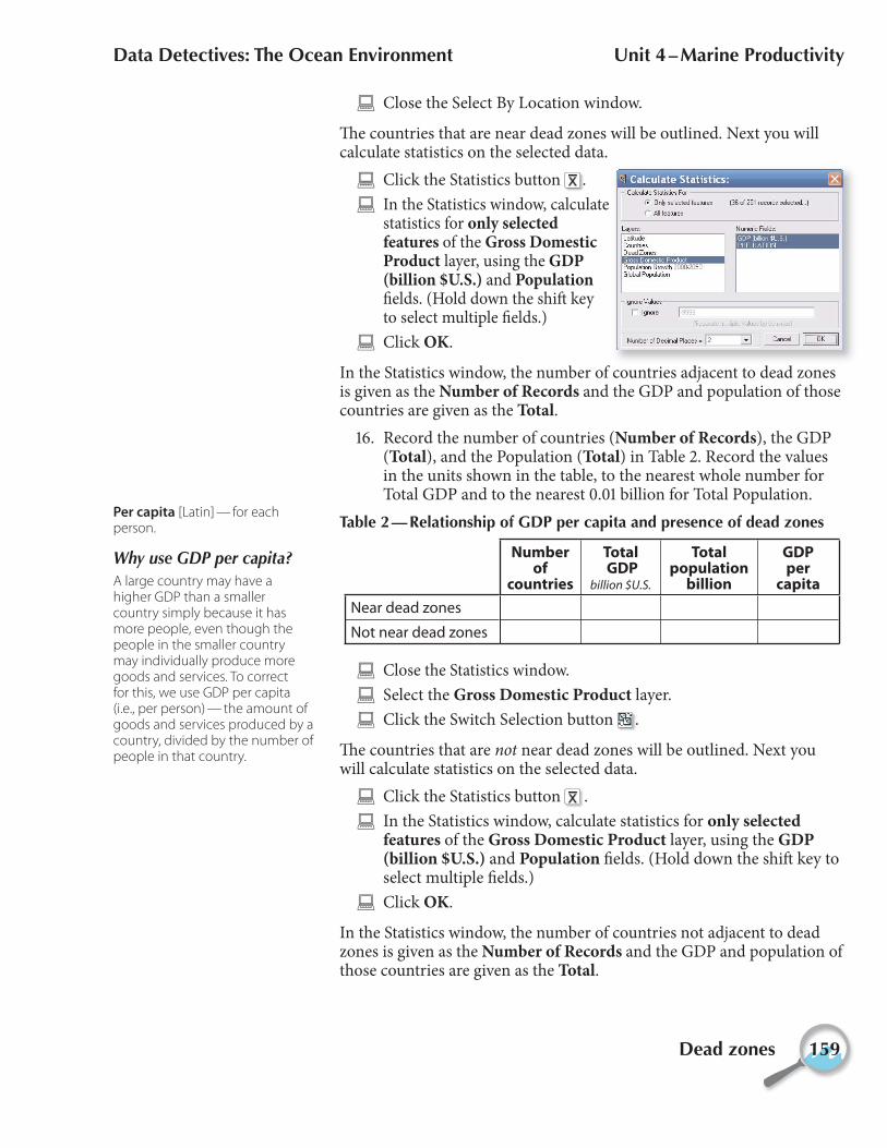
Click the Statistics button .

In the Statistics window, calculate statistics for only selected features of the Gross Domestic Product layer, using the GDP (billion $U.S.) and Population fi elds. (Hold down the shift key to select multiple fi elds.)

Click OK.

In the Statistics window, the number of countries adjacent to dead zones is given as the Number of Records and the GDP and population of those countries are given as the Total.

16. Record the number of countries (Number of Records), the GDP (Total), and the Population (Total) in Table 2. Record the values in the units shown in the table, to the nearest whole number for Total GDP and to the nearest 0.01 billion for Total Population.

Table 2 — Relationship of GDP per capita and presence of dead zones

Number of

countries

Total GDP

billion $U.S.

Total population

billion

GDPper

capita

Near dead zones

Not near dead zones

Close the Statistics window.

Select the Gross Domestic Product layer.

Click the Switch Selection button .

Th e countries that are not near dead zones will be outlined. Next you will calculate statistics on the selected data.

Click the Statistics button .

In the Statistics window, calculate statistics for only selected features of the Gross Domestic Product layer, using the GDP (billion $U.S.) and Population fi elds. (Hold down the shift key to select multiple fi elds.)

Click OK.

In the Statistics window, the number of countries not adjacent to dead zones is given as the Number of Records and the GDP and population of those countries are given as the Total.

Why use GDP per capita?A large country may have a higher GDP than a smaller country simply because it has more people, even though the people in the smaller country may individually produce more goods and services. To correct for this, we use GDP per capita (i.e., per person) — the amount of goods and services produced by a country, divided by the number of people in that country.

Per capita [Latin] — for each person.


160 Dead zones

17. Record the number of countries, GDP, and population values for countries not adjacent to dead zones in Table 2 on the previous page.


18. Calculate the GDP per capita both for the countries near dead zones and for the countries not near dead zones, and record them in Table 2. (Divide the Total GDP by the Total Population.)

19. How do the GDP per capita values diff er for the two groups of countries?

20. How might GDP be a better indicator than population for the future development of dead zones?

In 2005, the world’s population was about 6.1 billion people. By 2050, it is expected to increase to 8.9 billion, with the largest growth in countries having low GDP per capita.

21. If the total global GDP — the sum of all the goods and services produced by all nations — increases at a similar rate, what eff ect do you think it will have on the size and location of dead zones?




Searching for solutions 161

Searching for solutionsWrap-up 4.5

Th e Gulf of Mexico is suff ering from the eff ects of industrial and agricultural pollution, population growth, and urban development. Th e Gulf receives 1.1 trillion m3 (300 trillion gallons) of runoff each year that contains a vast collection of pollutants originating from factories, hog-waste ponds, heavily fertilized farms, golf courses, and residential lawns, as well as oily grime from urban runoff .

Although these chemicals pose serious health hazards, the added nutrients pose the biggest problem, triggering a series of events leading to the formation of the Mississippi River dead zone. Excess nutrients have also been implicated in the deaths of coral reefs, decline of sea-grass beds, occurrence of red tides, and declining health of estuaries around the Gulf of Mexico.

1. Describe the cascade of events that leads to the formation of a dead zone, beginning with the addition of excess nutrients. Be sure to discuss how the presence of excess nutrients aff ects primary producers and other consumers in the food web.

Although the Mississippi River dead zone is the largest in the U.S., it is not the only one. Next you will determine the eff ect your community has on dead zones off the U.S. coasts.

What are red tides?Red tides are caused by seasonal reproductive surges, or blooms, of certain species of marine algae. During a bloom, colored pigments in these tiny one-celled plants discolor the ocean surface, giving it a reddish-brown appearance.

Most of these algae species are harmless, but a few produce potent chemical neurotoxins (poisons that aff ect the nervous system). These toxins cause widespread fi sh kills, contaminate shellfi sh, and can be deadly to humans and other animals that eat contaminated seafood.

Estuary — body of water where a river meets the ocean, mixing fresh river water with ocean water.


162 Searching for solutions



In the Table of Contents, right-click the U.S. Dead Zones data frame and choose Activate.

Expand the U.S. Dead Zones data frame.

Th is data frame shows the major rivers and watersheds in the contiguous U.S. Find the approximate location of your city or town on the map.

Using the Zoom In tool , locate and zoom in on the region you live in.

Click the Identify tool .

In the Identify Results window, select the Major Rivers layer from the drop-down menu.

Next, click on the major river nearest to your town.

2. What major river carries runoff from your region to the ocean?

In the Identify Results window, select the Major Watersheds layer from the drop-down menu.

Click on the watershed in which your town is located.

3. What is the name of the major watershed in which your town is located?


Science can tell us a lot about how dead zones are created and their impact on the environment. However, cleaning up dead zones requires signifi cant changes in our behavior as a society.

Search the Internet to learn more about the sources of pollution, the economic impact of dead zones, and the technological solutions to the problem; then answer the questions on the following page. Some example Web sites are provided on page 164 to help you begin.


Searching for solutions 163

4. Discuss how your city or town contributes to the formation of a dead zone. Th ink about local residential, commercial, agricultural, and industrial practices.

5. Discuss how you might mitigate the negative impact of some of these activities.

Mitigate — to make less severe.


164 Searching for solutions

Web sites on the Gulf of Mexico dead zonePotential Solutions for Gulf of Mexico’s “Dead Zone” Explored Discusses the impact of the dead zone as well as ecological and

technological approaches to reducing the nutrient fl ow into the ocean.

http://researchnews.osu.edu/archive/hypoxia.htm

Environmental Literacy Council Provides an overview of the problem and links to major

government and research groups investigating the problem and solutions.

http://www.enviroliteracy.org/article.php/1128.html

National Center for Appropriate Technology (NCAT) Discusses causes of hypoxia and the human activities that

contribute to it. Also discusses approaches to reducing nutrient fl ow to the ocean.

http://www.ncat.org/nutrients/map.html

The Gulf of Mexico Dead Zone and Red Tides Discusses the eff ect of the dead zone on the quality and quantity

of fi sh and seafood stocks in the Gulf of Mexico.

http://www.tulane.edu/~bfl eury/envirobio/enviroweb/DeadZone.htm

Deep Trouble — The Gulf in Peril Series of articles in the Naples (Florida) Daily News outlining all

the issues facing the Gulf of Mexico and potential solutions.

http://web.naplesnews.com/deeptrouble/index.html


Media Viewer shortcutsTo open these Web pages from within ArcMap, click the Media Viewer button and choose the appropriate entry from the list of Web sites.

Exploring Solutions

Dead Zone Research

Hypoxia

Red Tides

Gulf in Peril

unit 4 marine productivity - cengage · pdf fileth us, scientists ... chlorophyll contained in...

Documents