university of southampton research repository eprints...
TRANSCRIPT

University of Southampton Research Repository
ePrints Soton
Copyright © and Moral Rights for this thesis are retained by the author and/or other copyright owners. A copy can be downloaded for personal non-commercial research or study, without prior permission or charge. This thesis cannot be reproduced or quoted extensively from without first obtaining permission in writing from the copyright holder/s. The content must not be changed in any way or sold commercially in any format or medium without the formal permission of the copyright holders.
When referring to this work, full bibliographic details including the author, title, awarding institution and date of the thesis must be given e.g.
AUTHOR (year of submission) "Full thesis title", University of Southampton, name of the University School or Department, PhD Thesis, pagination
http://eprints.soton.ac.uk
University of Southampton
Faculty of Engineering and the Environment
Investigation of Hybrid Systems for Diesel Powered Ships
By
Eleftherios K. Dedes
Thesis submitted for the Degree of Doctorate of Philosophy
July 2013


Abstract
I
Abstract
The combination of a prime mover and an energy storage device for reduction of fuel
consumption has been successfully used in the automotive industry. The potential of a load
levelling strategy and the energy management optimisation through the use of a Hybrid
Diesel propulsion system for ocean going ships is investigated. The goal of Diesel Hybrid
systems is to reduce exhaust gas emissions by reducing fuel oil consumption though an
introduction of an energy storage medium. Part of the research is based on operational
data for a shipping fleet containing all types of bulk carriers. The engine loading and energy
requirements are estimated and the sizing of suitable propulsion and the battery storage
system is proposed. The changes in overall emissions are estimated and the potential for
fuel savings is identified. The emission estimation is made by applying a bottom up
approach, and the use of fuel based factors. The thesis includes an assessment of the
calculation error imposed by the usage of fuel-based factors, and a determination of the
uncertainty in the approximation of global shipping emissions is made. Constructional and
volume constraints are identified and a concept feasibility is performed.
The thesis demonstrates the use of developed ship voyage simulator, which is a
time domain quasi-steady simulation tool. The system components of the Hybrid and the
conventional machinery system are modelled, the weather characteristics and the hull-
fluid interaction are implemented in a modular, scalable and expandable manner. Using
the simulation tool, an assessment of simulated bottom up approach with the results of the
IMO formula is presented for a number of examined voyages. Moreover, simulator outputs
of the propulsive demand are fed to the optimisation algorithm, which is based on the
equivalent cost minimisation strategy. In addition, a pseudo multi-objective optimisation
algorithm for CO2 and PM reduction is also presented. The results indicate that the ship
simulator estimates shipping emissions with a significantly smaller error than the adopted
formulae of the IMO.
The hybrid solution for diesel powered ships is under specific scenarios financially
viable, and the fuel savings based on the statistical analysis are notable when ageing of the
engines and performance deterioration models are included. Nevertheless, when the
optimised performance of the Hybrid power layouts is compared to optimally tuned
engines at ISO conditions, instead of the actual prime mover performance, the the fuel
saving potential for auxiliary loads is reduced and also leads to non-feasible results for
propulsive loads. Nonetheless, the Hybrid power systems permit the use of sophisticated
prime mover energy management for both propulsive and auxiliary loads. This proved to
lead to notable fuel savings for the combined shipboard power trains.

II
(Page left intentionally blank)

Table of Contents
III
Table of Contents
Abstract ................................................................................................................................ I
List of Figures .................................................................................................................. VII
List of Tables ...................................................................................................................... XI
Nomenclature ................................................................................................................... XV
Abbreviations ............................................................................................................... XXIII
Declaration of Authorship ............................................................................................. XXV
Acknowledgements ..................................................................................................... XXVII
1 Introduction ........................................................................................... 1
1.1 Background ........................................................................................................... 1
1.2 Aim and Objectives ............................................................................................... 4
1.3 Dry bulk sector ...................................................................................................... 6
1.4 Layout of thesis ..................................................................................................... 8
2 Shipping Emissions, Policy and Energy Efficiency ................................. 11
2.1 Diesel engine operation ....................................................................................... 12
2.2 Methods for estimating ship emissions .............................................................. 17
2.3 Improving the energy efficiency of the vessels ...................................................28
2.4 Operational and port methods to reduce emissions ........................................... 29
2.5 Technical measures to reduce emissions ............................................................ 31
Rudder modifications .................................................................................. 31
Improvement of propeller up flow and down flow ...................................... 31
Minimisation of ship total resistance .......................................................... 33
Improvements in the propulsion machinery ............................................... 35
2.6 Chapter summary ............................................................................................... 40
3 Hybrid Power Systems .......................................................................... 41
3.1 Implementation of Hybrid Power Systems ......................................................... 41
Selection of suitable prime movers .............................................................. 42
Selection of suitable energy storage medium .............................................. 44

Table of Contents
IV
Selection of miscellaneous electrical components ....................................... 49
Hybrid power system layouts ...................................................................... 52
Hybrid power system component efficiency ............................................... 55
3.2 Conceptual case based on voyage statistical analysis ......................................... 64
Statistical power analysis ............................................................................. 64
Sizing the Hybrid power system .................................................................. 70
3.3 Feasibility analysis .............................................................................................. 73
Operational feasibility based on voyage analysis ........................................ 73
Financial feasibility based on voyage analysis ............................................. 76
Technical feasibility assessment .................................................................. 79
3.4 Chapter summary ............................................................................................... 88
4 Mathematical Modelling ....................................................................... 89
4.1 Ship – Environment interaction modelling ........................................................89
Calm water resistance approximation .........................................................89
Added resistance due to wind and waves .................................................... 94
Hydrodynamic induced forces ................................................................... 101
Wind induced resistance ............................................................................ 104
The Propulsor and Governor models ......................................................... 106
Main Engine simple model ........................................................................ 110
Miscellaneous calculations ........................................................................ 110
Generation of environmental parameters .................................................. 112
4.2 Energy storage system........................................................................................ 115
4.2.1 Sizing of battery banks ................................................................................ 115
4.2.2 Battery models ............................................................................................ 117
4.3 Optimisation of Machinery Operation ............................................................... 121
4.3.1 Pseudo multi-objective optimisation algorithm ........................................ 123
4.3.2 Equivalent Cost Minimisation Strategy (ECMS) ....................................... 136
4.4 Implementation example – Mathematical representation ............................... 146
4.4.1 Ship – Environment interaction ................................................................ 146

Table of Contents
V
4.4.2 Coupling power profile and Hybrid system Optimisation ......................... 149
4.5 Chapter summary .............................................................................................. 150
5 Ship Voyage Simulator......................................................................... 151
5.1 Simulation implementation .............................................................................. 152
5.1.1 Input data blocks ....................................................................................... 155
5.1.2 Calm water resistance block ...................................................................... 157
5.1.3 Propeller block ........................................................................................... 160
5.1.4 Wind induced resistance blocks ................................................................. 161
5.1.5 Added resistance blocks ............................................................................. 163
5.1.6 Rudder and Drift resistance block ............................................................. 166
5.1.7 Engine interpolation block ........................................................................ 168
5.1.8 Kinetic Battery Model block ...................................................................... 170
5.1.9 LP Optimisation block ................................................................................ 171
5.1.10 Weather routing capability ........................................................................ 172
5.2 Simulink block and optimisation algorithm test cases ..................................... 173
5.2.1 Calm water resistance block test ................................................................ 173
5.2.2 Propeller block test .................................................................................... 176
5.2.3 Wind induced loads block test ................................................................... 180
5.2.4 Added resistance block test ....................................................................... 182
5.2.5 Non-linear optimisation test...................................................................... 187
5.3 Implementation example – Simulation representation ................................... 188
5.4 Chapter summary .............................................................................................. 193
6 Simulation and Optimisation Results ................................................. 195
6.1 Ship Voyage simulation ..................................................................................... 195
Voyage simulation using 24 hour time step .............................................. 197
Voyage simulation using 2h time step ...................................................... 203
6.2 Optimisation of propulsive and auxiliary machinery ...................................... 206
Prime movers operating at normal running conditions ........................... 206
Sensitivity analysis for D-A1 and D-B layouts ........................................... 214

Table of Contents
VI
Prime movers operating at special running conditions ............................. 218
6.3 Chapter summary .............................................................................................. 222
7 Conclusions ........................................................................................ 225
7.1 Discussion ......................................................................................................... 232
7.2 Implications for future application ................................................................... 234
References ........................................................................................................................ 235
Appendix I ............................................................................................................................. i
Appendix II ......................................................................................................................... vi
Appendix III ......................................................................................................................... x
Appendix IV ...................................................................................................................... xiii

List of Figures
VII
List of Figures
Chapter 1
Figure 1.1: World fleet CO2 emission share in m. tonnes per vessel category, year............ 2
Chapter 2
Figure 2.1: Specific Fuel Oil Consumption curves and specific NOx curves for 2-stroke and
4-stroke Diesel engines ...................................................................................................... 15
Figure 2.2: Comparison of ‘Activity’ method of power based factors and fuel based factors
with LMT assumptions, for CO2 emissions ....................................................................... 22
Figure 2.3: Comparison of ‘Activity’ method of power based factors and fuel based factors
with LMT assumptions, for SOx emissions ........................................................................ 23
Figure 2.4: Comparison of ‘Activity’ method of power based factors and fuel based
factorswith LMT assumptions, for NOx emissions ............................................................ 23
Chapter 3
Figure 3.1: Required propulsive power and propeller RPM for resistance profiles .......... 42
Figure 3.2 Hybrid Diesel-Mechanical System, layouts D-A, D-B or D-C .......................... 53
Figure 3.3: Hybrid- All Electric Ship Propulsion layout (D-A2 concept) .......................... 54
Figure 3.4: Line Diagram of the proposed D-A2 concept .................................................. 54
Figure 3.5: Experimental Sodium Nickel-Chloride battery efficiency mesh versus Depth of
Discharge and Discharge Current ...................................................................................... 58
Figure 3.6: Experimental curve of Sodium Nickel-Chloride battery efficiency versus charge
current................................................................................................................................ 59
Figure 3.7: Electric Motor/ Generator efficiency versus loading ..................................... 60
Figure 3.8: Specific Fuel Oil Consumption of Auxiliary generator sets ........................... 60
Figure 3.9: Specific Fuel Oil Consumption curves for Full, Part and Normal Loads ........ 62
Figure 3.10: Estimated engine loading for laden and ballast voyages............................... 66
Figure 3.11: Mean engine loading for laden and ballast voyage ........................................ 67
Figure 3.12: Requested energy per day for every vessel and voyage type .........................68
Figure 3.13: Example of energy fluctuation difference for laden and ballast Voyage ....... 69
Figure 3.14: Energy charging/discharging during at sea operation, from voyage’s working
point and application of regression analysis ..................................................................... 72

List of Figures
VIII
Chapter 4
Figure 4.1: Wave and wind angles of attack in degrees and description terminology ...... 97
Chapter 5
Figure 5.1: Ship Voyage Simulator flow chart.................................................................. 153
Figure 5.2: Simulation block minimum response time ................................................... 154
Figure 5.3: Data input blocks and signal generators in Simulink environment.............. 156
Figure 5.4: Representation of Holtrop Mennen resistance and approximation of
hydrodynamic coefficients block in Simulink environment ............................................ 158
Figure 5.5: Representation of the Hollenbach resistance block in Simulink .................. 159
Figure 5.6: Representation of Propeller block in Simulink .............................................. 161
Figure 5.7: Representation of Wind induced forces block in Simulink ........................... 162
Figure 5.8: Representation of Added resistance block in Simulink ................................ 163
Figure 5.9: Representation of Series 60 added resistance block in Simulink ................. 165
Figure 5.10: Representation of Rudder and Drift resistance block in Simulink ............. 167
Figure 5.11: Representation of Engine interpolation block in Simulink ......................... 169
Figure 5.12: Representation of KiBaM battery model block in Simulink ........................ 170
Figure 5.13: Representation of Linear Programming optimisation block in Simulink .... 171
Figure 5.14: Comparative analysis of multiple approximation methods and full scale
resistance model data ...................................................................................................... 174
Figure 5.15: Comparative analysis of resistance approximation and model test results for
design draft and speed range of 11 – 16 knots ................................................................. 175
Figure 5.16: Comparative analysis of B-series approximation and actual propeller data176
Figure 5.17: Propeller engine interaction for 2 resistance methods and for B-series
approximation compared to actual propeller performance data .....................................177
Figure 5.18: Simulink representation for Calm water resistance, propeller and propeller-
engine interaction comparative analysis ......................................................................... 179
Figure 5.19: Comparative analysis of wind induced loads methods ................................ 180
Figure 5.20: Simulink representation for wind induced loads comparative analysis ..... 181
Figure 5.21: Comparative analysis of Aertssen and Kwon added resistance models for
constant speed, head waves and increasing sea state ...................................................... 182
Figure 5.22: Comparative analysis of Towsin and Kwon and Aertssen models for head
waves, increasing Beaufort number and progressively increased speed. ........................ 183
Figure 5.23: Daily mean Beaufort Number and vessel speed versus voyage day ............ 184
Figure 5.24: Added Resistance comparative analysis of Kwon and Series 60 methods . 185
Figure 5.25: Detail of Added Resistance comparative analysis ....................................... 185
List of Figures
IX
Figure 5.26: Simulink representation for added resistance comparative analysis ......... 186
Figure 5.27: Comparison of Conventional, Hybrid engine outputs and battery power .. 187
Figure 5.28: Battery Depth of Discharge versus simulation time ................................... 188
Chapter 6
Figure 6.1: Ship Simulator representation in Simulink environment ............................. 196
Figure 6.2: Resistance breakdown for a 32 laden voyage ................................................ 198
Figure 6.3: Simulated versus ‘as measured’ fuel consumption ....................................... 199
Figure 6.4: Simulated propeller efficiency ..................................................................... 200
Figure 6.5: Simulated main engine loading ..................................................................... 201
Figure 6.6: Comparison of resistance curves for design laden condition ....................... 201
Figure 6.7: Simulated M/E loads in re-analysed ballast voyages ................................... 202
Figure 6.8: Simulated Main Engine loading using 2h weather generation model ......... 204
Figure 6.9: Vessel speed and significant wave height correlation applying 2h weather
generation model ............................................................................................................ 204
Figure 6.10: Simulated Wind direction using 2h weather generation model .................205
Figure 6.11: Propulsive power versus speed for laden and ballast voyages .................... 206
Figure 6.12: Auxiliary Power demand for 48 hours......................................................... 207
Figure 6.13: Power split and comparison for 14.4MWh capacity ................................... 208
Figure 6.14: Power split and comparison for 2MWh capacity ....................................... 209
Figure 6.15: Operating principle of D-C Hybrid power layout ........................................ 213
Figure 6.16: Power split and comparison for 2MWh capacity and up-scaled output ..... 219
Figure 6.17: Power split and comparison for 2MWh capacity and down-scaled output 220
Appendices
Appendix Figure 1: Energy profile regression analysis for Handysize type ........................ x
Appendix Figure 2: Energy profile regression analysis for HandyMax type ...................... xi
Appendix Figure 3: Energy profile regression analysis for Panamax type ......................... xi
Appendix Figure 4: Energy profile regression analysis for Capesize type......................... xii
Appendix Figure 5: Steam Cycle with superheating and one expander .......................... xxii
Appendix Figure 6: Nuclear steam cycle with two expanders, reheating ........................ xxii
Appendix Figure 7: Nuclear Hybrid AES system ............................................................ xxvi
Appendix Figure 8: Average electric power demand for laden and ballast voyages ....... xxx
Appendix Figure 9: Shipboard energy audit measurements of A/E loads ..................... xxxi
Appendix Figure 10: Battery Depth of Discharge in Hybrid Nuclear layout ................ xxxiv
Appendix Figure 11: Power split for Nuclear Hybrid configuration .............................. xxxv

X
(Page left intentionally blank)

List of Tables
XI
List of Tables
Chapter 1
Table 1.1: Ship type description ........................................................................................... 7
Chapter 2
Table 2.1: Emission factors for low speed engines (TIER I) .............................................. 19
Table 2.2: Comparison and calculation of fuel and power based factors implied error.... 21
Table 2.3: Examined set of voyages for emission factor evaluation ................................. 22
Table 2.4: Compatibility of hydrodynamic devices ........................................................... 36
Table 2.5: Synopsis of operational practices aiming to energy efficiency ......................... 37
Table 2.6: Synopsis of technical practices aiming to energy efficiency ............................. 39
Chapter 3
Table 3.1: Energy density and cost per battery type .......................................................... 46
Table 3.2: Hybrid System component efficiencies ............................................................ 56
Table 3.3: Auxiliary Generator set characteristics ............................................................. 61
Table 3.4: Characteristics of examined ‘parent’ Main Engines. ........................................ 62
Table 3.5: Sample of Daily performance report (‘noon report’) ........................................ 65
Table 3.6: Working Point of equivalent propulsion system .............................................. 69
Table 3.7: Suitable Diesel generator sets (Tier II) ............................................................. 71
Table 3.8: Storage medium required energy capacity and maximum power output ........ 72
Table 3.9: Potential fuel savings, for D-A2 and D-B layouts for static efficiencies ........... 74
Table 3.10: Extrapolated for the global bulker fleet potential emission savings ............... 75
Table 3.11: Internal Rate of Return for conceptual Hybrid power layout ......................... 78
Table 3.12: Hybrid energy requirements according to ship type...................................... 80
Table 3.13: Vessel added weight due to propulsion system retrofitting and installation of
energy storage medium......................................................................................................82
Table 3.14: Loading Conditions of examined Post-Panamax bulk carrier ........................ 83
Chapter 4
Table 4.1: Applicability range of calm water resistance approximation methods ............. 93
Table 4.2: Aertssen values for m and n coefficients .......................................................... 96
Table 4.3: Henschke sea description and correlation with Beaufort number ...................98
List of Tables
XII
Table 4.4: Static and rudder force and yawing moment coefficients estimates .............. 103
Table 4.5: Sample of data interpretation for ship voyage simulation ............................. 147
Chapter 5
Table 5.1: Holtrop Mennen resistance block inputs and outputs .................................... 157
Table 5.2: Hollenbach resistance block inputs and outputs ............................................ 160
Table 5.3: Propeller block inputs and outputs ................................................................. 160
Table 5.4: Wind induced loading block inputs and outputs ............................................. 161
Table 5.5: Aetrssen and Kwon block inputs and outputs ................................................ 164
Table 5.6: Series 60 added resistance approximation block inputs and outputs ............ 165
Table 5.7: Rudder and Drift resistance approximation block inputs and outputs .......... 166
Table 5.8: Engine Interpolation block inputs and outputs.............................................. 168
Table 5.9: Kinetic Battery Model block inputs and outputs ............................................. 171
Table 5.10: LP optimisation block inputs and outputs .................................................... 172
Table 5.11: Percentage of sailing time in specific Beaufort numbers .............................. 184
Table 5.12: Set of geometrical information for heavy ballast draft ................................. 189
Table 5.13: Wind speed regeneration matrix sample ...................................................... 190
Chapter 6
Table 6.1: Ship Simulation examined voyages and cargo quantity present .................... 197
Table 6.2: Simulated versus the ‘as measured’ fuel consumption ................................... 199
Table 6.3: Re-analysis of the ballast voyage fuel consumptions .................................... 203
Table 6.4: Effect of logic and installed capacity on the amount of fuel savings ............. 209
Table 6.5: Effect of tref and sampling time in savings percentage for 24h sample .......... 210
Table 6.6: Effect of tref and sampling time in savings percentage for 48h sample ........... 211
Table 6.7: Power Split for layout D-C for propulsive load demand ................................. 212
Table 6.8: Power Split for layout D-C for propulsive load and auxiliary demand .......... 214
Table 6.9: Fuel savings with battery degradation for 48h sample with Tref = 48h .......... 215
Table 6.10: Fuel savings with battery degradation for 24h sample with Tref = 72h......... 215
Table 6.11: Battery degradation model with marginal subcomponent efficiency ........... 216
Table 6.12: Sensitivity analysis for D-B Hybrid power layout ......................................... 217
Table 6.13: Power split and battery DoD for layout D-B and for downscaled M/E ........ 221

List of Tables
XIII
Appendices
Appendix Table 1: Electric Components in E/R of a modern cruise ship .......................... vi
Appendix Table 2: Comparison of propulsion technologies.............................................. vii
Appendix Table 3: Weight, volumes of machinery equipment, tanks and rooms in engine
room for 2-stroke Diesel propulsion system ..................................................................... vii
Appendix Table 4: Global fleet (until 2007) and power trends per vessel category ........ xvi
Appendix Table 5: Small Modural Reactor principal characteristics ............................. xviii
Appendix Table 6: Characteristics of civil reactor commercial designs ........................... xix
Appendix Table 7: Electric load analysis for Post-Panamax vessels .............................. xxix
Appendix Table 8: Power Split and battery DoD of Nuclear Hybrid system ............... xxxvi

XIV
(Page left intentionally blank)

Nomenclature
XV
Nomenclature
: Displacement volume of the ship [m3]
a : Correction factor for CB and Froude number (Kwon, 2008) [-]
A : Number of fissions [-]
ABT : Transverse area of the bulbous bow [m2]
AE/Ao : Expanded blade area ratio [-]
AF : Frontal projected area [m2]
Ai : Coefficients determined in Isherwood (1974) [-]
AL : Lateral projected area of the ship [m2]
An : Wave amplitude [-]
AR : Rudder area [m2]
AT : Transverse projected area of the ship [m2]
ATR : Immersed transom area [m2]
aw : shape factor of Weibul/ Rayleigh probability density functions [-]
B : Breadth of the ship [m]
Batcap : Battery Energy Capacity [kWh]
be : Specific Fuel Oil Consumption at examined load [g/kWh]
Bi : Coefficients determined in Isherwood (1974) [-]
bkW : Engine’s break Power [kW]
BN : Beaufort number [-]
C : Distance from bow of centroid to the AL [m]
CA : Correlation allowance coefficient in Hotrop (1981) [-]
CB : Block coefficient [-]
CF : Frictional resistance coefficient ITTC 1957 [-]
CF A/E : A/E fuel carbon content [-]
CF M/E : M/E fuel carbon content [-]
CF : Friction coefficient [-]
CFi : Fuel type coefficient [-]
Ci : Coefficients determined in Isherwood (1974) [-]
cKB : Constant dependent on the battery technology [-]
Cn : Coefficient (Oosterveld and Oossanen, 1975) [-]
Cnom : Nominal battery capacity [MWh]
CP : Prismatic coefficient [-]
CRi : Correction factors imposed by engine manufacturers [-]
CRLCVF : Correction for fuel oil low calorific value [-]

Nomenclature
XVI
Cstern : Stern type as described in Holtrop and Mennen (1981) [-]
CV : Viscous resistance coefficient [-]
CWP : Water plane coefficient [-]
D : Drought of the ship [m]
Di : Sailed distance [n. m.]
DoDin : Battery Depth of Discharge at simulation time step [%]
DoDt-1 : Battery Depth of Discharge at previous simulation time step [%]
Dp : Propeller diameter [m]
dV : Voltage drop/ excess during discharging/ charging [V]
DWT : Vessels deadweight [tonnes]
E0 : Electromotive force or open-circuit voltage of cell [V]
Ebat : Installed Battery Energy Density [kWh]
F : Fetch distance [km]
fci : Correction factor to account ship specific design elements [-]
feff : Availability factor of innovative energy saving technology [-]
fi : Coefficients for E/R volume approximation (SNAME, 1990) [-]
fj : Capacity factor for technical/regulatory limitation on capacity [-]
Fn : Froude number [-]
Fni : Froude number based on the immersion [-]
Fo : Oversizing factor and is determined by the designer [-]
FT : Turbulence scale [-]
fw : Non-dimentional deduction coefficient of sea condtions [-]
g : Acceleration of gravity [m/s2]
g(x) : Specific Fuel Oil Consumption curve [g/kWh]
h(x) : SFOC curve for type II Diesel Generator Set [g/kWh]
hB : Vertical position of ABT from the keel plane [m]
hi : Enthalpies at certain temperature and dryness [kJ]
hp : Enthalpy at condenser [kJ]
i : Operating current of battery on load [A]
J : Advance speed [-]
k : Coefficient determined by Hollenbach method [-]
k’ : Coefficient determined by Manwell et al. (2005) [-]
kBoss : Boss coefficient [-]
kBrac : Bracket coefficient [-]
KN : The surface drag coefficient equal [-]
KQ : Non-dimensional propeller torque coefficient [-]
KR : Rudder velocity distance corrective factor [-]

Nomenclature
XVII
kRudd : Rudder coefficient [-]
KT : Non-dimensional propeller thrust coefficient [-]
L : Equivalent ship length (Schneekluth and Bertram, 1998) [-]
LCB : Longitudinal Centre of Buoyancy [m]
lcb : LCB expressed in percentage from amidships [%]
LCG : Longitudinal Centre of Gravity [m]
LF : Engine load factor [-]
LOA : Length overall [m]
LOS : Length over surface determined in Hollenbach method [m]
LPP : Length between perpendiculars [m]
LWL : Length of waterline [m]
m : Steam mass flow [kg/m3]
Maxd.c : Battery Maximum Discharge current [A]
MCRA/E : Maximum Continuous Rating of Auxiliary Diesel Engine [kW]
MCRm : Maximum Continuous Rating of electric machine [kW]
MCRM/E : Maximum Continuous Rating of Main Diesel Engine [kW]
mf : Mass of injected fuel [kg]
MTC : Moment to change trim [tm]
MXG : Gust peak [m/s]
MXR : Ramp maximum value [m/s]
n : Revolutions of the propeller [rps]
N : Number of measurements [-]
N’uuδ : Static non-dimensional yawing moment coefficient [-]
N’uν : Static non-dimensional rudder yawing moment coefficient [-]
NBB : Number of Battery Banks [-]
NBoss : Number of bosses [-]
NBrac : Number of brackets [-]
nbs : Number of batteries in DC bus [-]
NFcons. : Nuclear fuel consumption [tonnes]
Noatoms : Required number of atoms to achieve the number of fissions [-]
NRcons. : Nuclear Reactor specific fuel depletion [g/kWh]
NRmax : Nuclear Reactor maximum power output [kW]
NRudd : Number of rudders [-]
P : Engine Output Power [kW]
p(x) : Power limit curve dictated by the Main Engine [kW]
P/D : Pitch to diameter ratio [-]
PA/E : A/E power output [kW]

Nomenclature
XVIII
PAES : All electric ship power demand [kW]
PB : Emergence of the bow [-]
Pdemand : Demanded power by the propulsion and/ or auxiliary loads [kW]
Peff : 75% Power of the M/E due to innovative technology [kW]
PM/E : M/E power output [kW]
Pprd : Produced Power [kW]
PPTI : Power Take In output power [kW]
PPTI : Power take off (PTI) power output [kW]
Preq. : Required Power [kW]
Ptotal : Required voyage propulsive power [kW]
PWHR : Waste heat recovery (WHR) equivalent power output [kW]
PWHR : Waste Heat Recovery system power output [kW]
q : Dynamic pressure of the apparent wind [Pa]
Q0 : Open water developed torque [Nm]
Q1 : Energy supplied by the nuclear reactor [kW]
QF : Fuel Chemical Power [kW]
R : Uniformly distributed number [0, 1] [-]
RA : Model-ship correlation [N]
RAPP : Appendage resistance [N]
RB : Pressure resistance of bulbous bow [N]
RF : Frictional resistance according to ITTC 1957 [N]
Ri : Internal resistance of the battery [Ω]
RPM : Engine Rotational speed [RPM]
RR : Residual Resistance [N]
RT : Total Resistance [N]
RTR : Pressure resistance of immersed transom stern [N]
RW : Wave-making and wave-breaking resistance [N]
SP : Perimeter of the lateral projection [m]
S : Wetted surface area [m2]
SAPP : Appendage wetted surface area [m2]
SFOCA/E : A/E specific fuel oil consumption [g/kWh]
SFOCM/E : M/E specific fuel oil consumption [g/kWh]
SFOCmin : Minimum SFOC of Auxiliary Engine [g/kWh]
SFOCmin : Minimum SFOC of Diesel Generator Sets [g/kWh]
Sn : Coefficient (Oosterveld and Oossanen, 1975) [-]
SoCref : Reference Battery State of Charge, user defined [%]
SoCt : Battery State of Charge at simulation time t [%]

Nomenclature
XIX
Stotal : Wetted surface area approximated by Hollenbach method [m2]
T : Developed thrust [N]
t : Thrust deduction factor [-]
T0 : Open water developed thrust [N]
T1G : Gust starting time [s]
T1R : Ramp start time [s]
T2R : Ramp maximum time [s]
Tair : Air temperature [oC]
TG : Gust period [s]
tref : Reference time where the SoCt must be equal to SoCref [h]
tsim : Simulation elapsed time [h]
TW : Water temperature [oC]
un : Coefficients (Oosterveld and Oossanen, 1975) [-]
uw : Wind speed [m/s]
V : Vessel speed [m/s]
v : Ship’s lateral velocity [m/s]
V0 : Undisturbed fluid speed at propeller [m/s]
V1 : accelerated speed at the propeller disk [m/s]
V2 : accelerated speed downstream of propeller disk [m/s]
VA : Velocity of advance [m/s]
VBat : Battery Voltage [V]
VEP : Engine Room Volume [m3]
vn : Coefficients (Oosterveld and Oossanen, 1975) [-]
Vnominal : Battery Nominal Voltage [V]
VOP : DC bus voltage [V]
VR : Relative wind speed [m/s]
VR : Relative wind velocity [m/s]
Vref : Vessel desing/ reference speed [knots]
Vref : Vessel reference speed defined by IMO [knots]
VRR : Relative rudder velocity [m/s]
VWB : Base wind velocity [m/s]
VWG : Gust wind component [m/s]
VWN : Noise wind component [m/s]
VWR : Ramp wind component [m/s]
w : Wake friction [-]
w(x) : Battery Discharge/ Charge efficiency curves [-]
Wcargo : Weight of transported cargo [tonnes]

Nomenclature
XX
WFuel : Consumed fuel weight [tonnes]
WP : Work required at pressuriser [kW]
WT : Work in the Turbine [kW]
X : Distance between rudder and propeller [m]
Y’ccδ : Non-dimensional rudder force coefficient [-]
Y’uv δ : Vessel Hydrodynamic coefficient [-]
Y’uν : Non-dimensional static force coefficient [-]
Yi,o : Amount of available and bound charge [Ah]
z : Number of blades [-]
β : scale factor of Weibul probability density function [-]
Γ : Gamma function [-]
Δ : Vessel displacement [tonnes]
δB : Coefficient determined in Blendermann (1994) [-]
Δtsim : Simulation time step [h]
ε : Wind angle of attack [rad]
(ηc)a : Concentration polarisation at anode and cathode [-]
(ηc)c : Concentration polarisation at anode and cathode [-]
(ηct)a : Activation polarisation or charge-transfer overvoltage at anode [-]
(ηct)c : Activation polarisation or charge-transfer overvoltage at cathode [-]
ηc : Propulsion converter efficiency [-]
ηconv. : Propulsion converter efficiency [-]
ηg : Gearbox/ clutch efficiency [-]
ηgen : Electric generator efficiency [-]
ηisHP : High Pressure turbine isentropic efficiency [-]
ηisLP : High Pressure turbine isentropic efficiency [-]
ηloss : Electric conversion losses [-]
ηm : Electric motor efficiency curve [-]
ηmHP : High pressure turbo generator efficiency curve [-]
ηmLP : Low pressure turbo generator efficiency curve [-]
ηoverall : Turbine system overall efficiency [-]
ηR : Relative rotative efficiency [-]
ηRankine : Rankine cycle efficiency [-]
ηreactor : Nuclear reactor efficiency [-]
ηT/F : Propulsion transformer efficiency [-]
ηT/F,inv : Battery Transformer and inverter efficiency [-]
ηtrans : Conversion losses due to power transmission [-]
Θu : Fuel Oil Lower Calorific Value [kJ/kg]

Nomenclature
XXI
μ : Correlation factor defined by Kwon method [-]
μsw : Salt water kinematic viscosity [m2/s]
ξn : Uniformly distributed random variables between [0, 2π] [-]
ρair : Air density [kg/m3]
ρw : Water density [kg/m3]
φi : Random variable with uniform probability density [0, 2π] [-]
ω0 : Encounter frequency [rad/s]
1+k1 : Form factor of hull viscous resistance [-]

XXII
(Page left intentionally blank)
Abbreviations
XXIII
Abbreviations
AC : Alternative current
A/E : Auxiliary Diesel engine
AES : All electric ship
BSRA : British ship research association
BWR : Boiling water reactor
CO : Carbon monoxide
CO2 : Carbon dioxide
CODOG : Combined Diesel or gas
CODAG : Combined Diesel and gas
CPD : Continuous professional development
DC : Direct current
DWT : Deadweight
EC : Elementary carbon
ECA : Emission control area
ECMS : Equivalent cost minimisation strategy
EEDI : Energy efficiency design index
EEOI : Energy efficiency operational indicator
EGR : Exhaust gas recirculation
EPR : European pressurised reactor
E/R : Engine room
FEP : Full electric propulsion
FEU : Fifty-foot equivalent unit container
GCFR : Gas-cooled breeder reactor
GHG : Green house gasses
GTO : Gate turnoff thyristors
GUI : Graphical user interface
HC : Unburnt hydrocarbons
HEU : High enriched Uranium
HFO : Heavy fuel oil
HVAC : Heating, ventilation and air conditioning system
ICE : Internal combustion engine
IFEP : Integrated full electric propulsion
IGCT : Integrated gate-commutated thyristors
IMO : International maritime organisation

Abbreviations
XXIV
IRR : Internal rate of return
ISO : International standardisation organisation
ITTC : International towing tank conference
JIT : Just in time arrival
LCB : Longitudinal centre of buoyancy
LEU : Low enriched Uranium
LMFBR : Liquid metal cooled breeder reactor
LNG : Liquefied natural gas
LWBR : Light-water breeder reactor
M/E : Main Diesel engine
MARPOL : Marine pollution
MCR : Maximum continuous rating
MDO : Marine Diesel oil
MEPC : Marine environmental pollution committee
MSBR : Molten salt breeder reactor
NCR : Nominal continuous rating
NOx : Nitrogen oxides
OC : Organic compounds
OGV : Ocean going vessel
PHEV : Plug-in hybrid electric vehicle
PM : Particulate matter
PTI : Power take-in
PTO : Power take-off
PWR : Pressurised water reactor
RBMK : Reaktor Bolshoy Moshchnosti Kanalniy (Russian)
RPM : Rotations per minute
SCR : Selective catalytic reaction
SCRe : Silicon controlled rectifier
SFOC : Specific fuel oil consumption
SMES : Superconducting Magnetic Energy Storage
SMR : Small modular reactor
SOx : Sulphur oxides
TEU : Twenty-foot equivalent unit container
VSC : Voltage source converter
WED : Wake equalising duct
WIT : Water in Fuel technology
ZEBRA : Zero emission battery research activity

Declaration of Authorship
XXV
Declaration of Authorship
I, Eleftherios K. Dedes declare that the thesis entitled ‘Investigation of Hybrid Systems for
Diesel Powered Ships’ and the work presented in the thesis are both my own, and have
been generated by me as the result of my own original research. I confirm that:
this work was done wholly or mainly while in candidature for a research degree at this
University;
where any part of this thesis has previously been submitted for a degree or any other
qualification at this University or any other institution, this has been clearly stated;
where I have consulted the published work of others, this is always clearly attributed;
where I have quoted from the work of others, the source is always given. With the
exception of such quotations, this thesis is entirely my own work;
I have acknowledged all main sources of help;
where the thesis is based on work done by myself jointly with others, I have made clear
exactly what was done by others and what I have contributed myself;
parts of this work have been published as: E. K. Dedes, D. A. Hudson and S. R. Turnock
Modifications on the Activity based approach for accurate estimation of fuel
consumption from global shipping, Transportation Research Part D: Transport
and Environment, to be submitted, 2013c.
Diesel Hybrid systems for increase of fuel efficiency and reduction of exhaust
emissions from ocean going ships, Journal of Energy, to be submitted, 2013b.
Technical feasibility of Hybrid Powering systems to reduce emissions from bulk
carriers, IJME Transactions of RINA, 2013a.
Design and Simulation of Hybrid Powering Systems for Reduction of Fuel Oil
Consumption and Shipping Emissions, 1rst International MARINELIVE
Conference on ‘All Electric Ship’, NTUA, Athens, Greece, 2012b
Assessing the potential of hybrid energy technology to reduce exhaust emissions
from global shipping, Energy Policy 40, p.p. 204-218, 2012a

Declaration of Authorship
XXVI
…and S. Hirdaris. Possible Power Train Concepts for Nuclear Powered Merchant
Ships. LCS conference, Glasgow, Vol. 1 p.p. 263-273, University of Strathclyde,
2011.
Design of Hybrid Diesel-Electric Energy Storage Systems to Maximize Overall
Ship Propulsive Efficiency, 11th PRADS conference R.J. Brazil, Vol. 1 p.p. 703-713,
COPPE UFRJ, 2010
Signed:
Date: 22/07/2013

Acknowledgements
XXVII
Acknowledgements
Firstly, I want to express my deep appreciation to my academic supervisors Professor
Stephen Turnock and Dr Dominic Hudson who guided me with their expertise and most
importantly who supported me in some difficult decisions. I would like to express my
gratitude as well to Professor Ajit Shenoi for offering me a place at the Fluid Structure
Interactions Group and for his support.
Secondly, I would like to thank my parents Konstantinos and Chrysanthi for
encouraging me to continue my studies, apply for research post-graduate degree and for
supporting my decisions.
I wish to thank Foundation Propondis, Eugenides Foundation, Union of Greek
Ship Owners, Lloyd's Register UK and Lloyd’s Register Educational Trust for the financial
support of the research project throughout the three years of study. Especially I would like
to thank the chairman of Propondis Foundation Mr D. Diamantides and the director Mr
G. Baveas, Dr S. Hirdaris from Lloyds’ Register UK strategic R&D and the regional
manager of Hellenic Lloyds Mr. A. Poulovassilis.
Furthermore I would like to express my gratitude to the Technical and
Operational departments of the Greek shipping company which provided the data,
especially to the Technical Manager Mr P. Provias, to the superintendent engineers Mr A.
Giantsis, Mr P. Triantafylos and Mr G. Gavrilis and to the technical department of Carnival
Corporation and plc.
Additionally, I wish to thank to Dr R. Wills from Faculty of Engineering and the
Environment of University of Southampton, Dr M. Ioannou from Wartsila R&D Swiss and
Professor C. Frangopoulos, Associate Professor J. Prousalidis and Mr G. Georgiou from
National Technical University of Athens.
Personally I would like to thank my friend and superintendent engineer Mr P.
Georgakis for his support and his professional opinion in the aspects of actual shipping
operations. Finally but not of least importance, a special thanks to Ms V. Maseli for her
sincere support and her belief for the successful continuation of my studies.
With the oversight of my main supervisor Professor S. R. Turnock, editorial
advice by Ms D. Kapsali has been sought. No changes of intellectual content were made as
a result of this advice.

XXVIII
(Page left intentionally blank)

XXIX
To my parents
Chrysanthi and Konstantinos

XXX
(Page left intentionally blank)

Chapter 1
1
1 Introduction
1.1 Background
Approximately 80% of world trade by volume is carried by sea (UNCTAD 2008). In 2007
it is estimated that international shipping was responsible for approximately 870 million
tonnes of CO2 emissions, or 2.7% of global anthropogenic CO2 emissions. By way of
comparison, this level of emissions is between those of Germany and Japan for the same
year. Domestic shipping and fishing activity bring these totals to 1050 million tonnes of
CO2, or 3.3% of global anthropogenic CO2 emissions. Despite the undoubted CO2 efficiency
of shipping in terms of grammes of CO2 emitted per tonne-km, it is recognised within the
maritime sector that reductions in these totals must be made (IMO, 2009). Nonetheless,
exhaust emissions from global shipping contribute significantly to the total emissions of
the transportation sector (Corbett et al, 1999; Eyring et al., 2005). Eyring et al., (2010)
mention that NOx emissions are currently estimated to be around 15% of global
anthropogenic NOx emissions and 4-9% of SOx, respectively, and recent legislation is
aimed at reducing these emissions through the introduction of emission control areas and
requirements on newly built marine diesel engines (MARPOL, 2005). The expected
changes in CO2 emissions from shipping from 2007 to 2050 were modelled for the
International Maritime Organisation with reference to the emissions scenarios developed
for the UN IPCC. These scenarios are based on global differences in population, economy,
land-use and agriculture (IMO, 2009). The base scenarios indicate annual increases of CO2
emissions in the range 1.9-2.7%, with the extreme scenarios predicting changes of 5.2%
and -0.8%, respectively. The increase in emissions is related to predicted growth in
seaborne transport. If global emissions of CO2 are to be stabilised at a level consistent with
a 2°C rise in global average temperature by 2050, it is clear that the shipping sector must
find ways to stabilise, or reduce, its emissions – or these projected values will account for
12% to 18% of all total permissible CO2 emissions.
Carbon dioxide and Suplhur oxides emissions from world shipping are directly
related to the fuel consumption of the fleet. In 2007, approximately 277 million tonnes of
fuel were consumed by international shipping. Three categories of ship account for almost
two thirds of this consumption. The liquid bulk sector accounts for ~65 million tonnes
fuel/year, container vessels for ~55 million tonnes fuel/year and the dry bulk sector for
~53 million tonnes fuel/year (IMO, 2009). Figure 1.1 depicts the actual share of Carbon
dioxide per vessel category, which is the most important GHG emitted by ships. In
addition, nitrogen oxides and particulate matter is directly related to the engine fuel
efficiency and working point.

Introduction
2
From a ship-owner/ managing Company perspective, the shipping sector is facing
the severe consequences of global recession. Increased vessel capacity, which affects the
balance between supply and demand, had led the older or the most inefficient vessels to
be unchartered. The ones that remain into the trading play are subject to low income,
affecting the prosperity of the sector. For that reason, the IMO, on the one hand, and
shipping companies on the other (the former for the purpose of lowering emissions), are
seeking ways to further reduce fuel consumption, which is directly related to net income
and to total emissions. Working towards improved ship energy efficiency, shipyards have
adapted their approach to ship design for newly-built ships, mainly under pressure from
the adopted legislation of the IMO, the Energy Efficiency Design Index and from the
shipping companies, which now demand an energy efficient ship in order to maximise
their profit in the longer term.
Figure 1.1: World fleet CO2 emission share in million tonnes per vessel category, year (Psaraftis and Kontovas, 2009)
This thesis, deals with the complex problem of ship fuel consumption which is related to
the total emitted exhaust gasses, the accurate measurement of the emission percentages
and the thermodynamic efficiency of marine Diesel engines. The latter efficiency is directly
related to the operational envelope of each ocean going vessel. Therefore, a suitable
proposal to minimise fuel consumption, reduce fuel emissions and be able to be installed
on current and future designs should be found.
The combination of a prime mover and an energy storage device for the reduction
of fuel consumption has been successfully used in the automotive industry (Mohamed et
al., 2009) and has been shown to contribute to reduced CO2 emissions (Alvarez et al., 2010;

Chapter 1
3
Fontaras et al., 2008). The shipping industry has utilised this for conventional submarines
where no oxygen is present during dive conditions. The question to be raised is whether
the hybrid solution consisting of a Diesel prime movers and batteries is suitable as a
method of increasing fuel efficiency and consequently for emission reduction in marine
applications.
The main reason for investigating a potential solution that uncouples the
production and the demand is primarily because the optimisation of marine diesel engines
is aimed at reducing fuel consumption for a broad range of operations. This implies that
the tuning of engine parameters such as injection and valve timing, the selection of the
turbochargers are made for a wide range of operational conditions, especially for camshaft
controlled engines. However, this range affects the local efficiency and more suitable
components for smaller operational profiles are not installed (Kyrtatos, 1993). Marine
engines operate in changing conditions at sea due to vessel interaction with hydrodynamic
and wind induced loads. In addition, the operations department/ charterer voyage orders,
may include voyage deviations and speed alterations which is another factor that affects
the propulsion system operational point. In order to serve this operational envelope, the
designers optimise engines for a broad operational range; there is, however, a specific
optimised point of minimum fuel consumption for a given speed. Unfortunately, the
operation of the engine at that point or near that point is not always possible. Thus the
specific fuel oil consumption (SFOC) is increased and both the thermodynamic and the
mechanical efficiencies of the engine drop (Klein Woud and Stapersma, 2003).
The efficiencies of marine diesel engines have increased in recent decades
(Kyrtatos, 2009) and efforts are continuing to reduce specific fuel consumption and
exhaust pollutant gases, such as NOx and SOx and shoot (PM and smoke) but still, the
broad range of operational conditions limits their overall efficiency.
The use of work investigates hybrid power system topologies allows the propulsor
(propellers in ocean going fleet) to be uncoupled from the process of the production of
rotational speed and torque by the Diesel prime movers. This concept requires the
existence of an intermediate energy storage medium or a sophisticated energy
management system to deal with the power demand. A preliminary concept for battery
electric propulsion was made in Barabino et al. (2009). The Hybrid propulsion system was
initially discussed by Nilsen and Sørfonn (2009) by coupling a Diesel engine and Diesel
generator set in a system with the Power take off (PTO-PTI) feature, in order to switch
propulsion unit while sailing into emission control areas (ECAs). It was believed that it is
easier to switch fuel type without stopping by having a generator set supplying energy to
the propulsion, burning lighter fuel only. Moreover, de Vos and Versuijs (2010)
investigated the potential for a Hybrid tug vessel to operate at low loads using a fuel cell,
Introduction
4
and to use the installed Diesel engine when in tug operation, for emission reduction and
optimised use of the power trail inside the port.
Grimmelious et al. (2011) state that ships having short-term peaks or long periods
of very low load, benefit the most from Hybrid Power systems. However, it is argued
among the shipping industry that other types of vessels can benefit from hybrid (consisting
of energy storage and Diesel engines) concepts. The primary feasibility analysis of hybrid
power systems for slow speed vessels published by Dedes et al. (2010) demonstrated that
the potential application of Hybrid systems in bulk carrier vessels can be feasible. It has
been determined that Hybrid Power system that can apply load levelling in propulsion
loads, control the energy production by optimally loading the prime mover for the total
duration of the voyage, is promising and has yet to be performed. However, the concept of
retrofit slow speed vessels with All Electric Hybrid propulsion to minimise
electromechanical losses from and to the battery system proved to be inefficient (Dedes et
al., 2012a).
1.2 Aim and Objectives
The aim of this thesis is to investigate the use of a conventional Diesel Mechanical system
for main propulsion, incorporating a PTO/PTI module and an appropriate energy storage
medium. For a conventional ship, the objective is to produce the required energy at near
optimum conditions by finding the optimum power split between the Diesel Engine and
the hybrid module. For the system to have a high energy efficiency, the engine specific fuel
oil consumption (SFOC) has to be near the minimum value. The energy storage system or
the sophisticated energy management is responsible for covering the energy demand and
maintaining the optimum energy production. Energy management and load levelling
result in reductions of the total fuel bill. In addition, a decrease of sea margin, hence a
decrease of the size of the total installed power as the peak demands, can be covered by the
storage medium without affecting the overall fuel efficiency. Nevertheless, to apply load
levelling and/or reduce the power output of the Diesel prime movers, the Hybrid Power
concept uses devices capable of storing large amounts of energy for a non-uniform
charging/discharging time profile. Specific objectives are to:
i. Investigate different storage systems and identifies high temperature batteries
as the most promising solution with their low installation cost, high power
density and high recyclability. For the conventional Diesel or Diesel-electric
propulsion layouts, it is expected that this system will allow a more flexible
approach to the overall propulsion system, permitting further application of
external emission reduction techniques. The application of sustainable

Chapter 1
5
technologies (such as solar panels, wind turbines, etc.) as auxiliary installations
to the charging circuit of the storage system is also feasible.
ii. Process a set of actual operational data which consists of fuel consumption and
the actual vessel operation for a fleet of dry bulk carrier vessels. Calculation of
CO2, NOx and SOx emissions and estimation of the engine loading for laden and
ballast voyages is then possible. The statistical data provided the information
necessary to estimate the size of the storage medium and identify the
optimisation point of the propulsion engines using an overall daily energy
consumption approach.
iii. Consider the connection of batteries and operational parameters using a
suitable modelling and simulation approach using a systematic energy
approach. The selection of the prime mover is crucial for any potential changes
in cargo capacity or vessel displacement. The energy storage media and diesel
generators will not make major changes in the ship weight and longitudinal
distribution that would reduce the carrying capacity of the vessel. Preliminary
economic feasibility of the project is to demonstrated for a Diesel-Hybrid Power
layout.
iv. Develop a ship voyage analysis simulation in Matlab/Simulink® environment
in order to extrapolate the results and investigate the emission profile of the
global fleet for a number of actual and fictional scenarios. The simulator is built
in a modular, scalable and extendable manner so that the simulation library
could be updated with higher complexity models or with updates of the
mathematical implementation of the existing ones.
v. Assess the benefit of Hybrid Power using non-linear optimisation algorithms
based on the Equivalent Cost Minimisation Strategy (ECMS) of Guzzella and
Sciarretta (2005), and a pseudo multi-objective optimisation algorithm, with
the primary target of reducing fuel consumption when the storage medium is
not depleted and minimising the PM emissions while the system is in charging
mode. The algorithm is to incorporate laboratory efficiency data for the main
propulsion marine Diesel engine and for the auxiliary Diesel generator sets.
Moreover, the sea trial and model test data for the thrust deduction factor,
relative rotational efficiency and wake friction coefficient for the examined ships
were inserted in the calculations and the simulation. In addition, detailed
experimental efficiency curves for the selected battery type were used.
Furthermore, for the electrical components, with the exception of the electric
machine efficiency curve, static efficiency factors were used. Due to the fact that
the latter proved to be of the most importance in terms of the feasibility of the

Introduction
6
Hybrid Power system, a sensitivity analysis was performed and the results are
discussed in detail.
1.3 Dry bulk sector
This study concentrates on the dry bulk sector as one of the major contributors to CO2
emissions of international shipping and a key sector underpinning global seaborne trade.
Between 1986 and 2006 average annual growth in the transport of coal and iron ore was
greater than that in the transport of oil and oil products and outstripped global GDP
growth (IMO, 2009). Within the dry bulk sector, the vessel types commonly used may be
classified according to Table 1.1.
It may be noted that the design of Post-Panamax bulk carriers has significant
similarities with liquid carrying tankers of a similar size (commonly referred to as Aframax
tankers) and the conclusions are of relevance to this sector and directly applicable to this
design. Aframax tankers account for approximately one third of all tankers (Lloyds
Maritime Information Services, 2007). Moreover, the Post-Panamax vessel category is
making itself apparent due to the new widened Panama Canal. However, due to this novel
ship sub-category the question of their propulsive efficiency in off design conditions is a
topic of discussion among the designers. For that particular reason, the hybrid layout
presented in this thesis might be for up discussion with the ultimate aim of increasing
propulsive efficiency by focusing on their propeller engine matching.

Chapter 1
7
Table 1.1: Ship type description (Molland et al., 2012)
Bulk carrier type Dimensions Ship size (scantling)
Small Overall ship length up to approx 115 m Up to 10,000 dwt Handysize Scantling draught up to approx 10 m 10,000 – 35,000 dwt
Handymax Overall ship length max 190 m 35,000 – 55,000 dwt Panamax
Ship breadth equal to Overall ship length up to
Passing ship draught up to
32.2 / 32.3 m
289.6 m 12.04 m
60,000 – 80,000 dwt
Post Panamax (Small capes) Breadth approx 43 - 45 m for 120,000 - 180,000 dwt
80,000 – 120.000 dwt
Capesize 120– 200,000 dwt
VLBC – Very Large Bulk Carrier LOA above 300 m > 200,000 dwt
Oil Tanker type Dimensions Ship size (scantling)
Small Overall ship length up to approx. 115 m Up to 10,000 dwt
Handysize Scantling draught up to approx. 10 m 10,000 – 30,000 dwt
Handymax Overall ship length max 180 m 30000 – 50,000 dwt
Panamax Ship breadth equal to
Overall ship length up to Passing ship draught up to
max: 32.2 / 32.3 m
225 m (port facilities) 12.04 m
60,000 – 75,000 dwt
Aframax Breadth approx. 41 - 44 m 80,000 – 120.000 dwt
Suezmax Ship breadth equal to
Drought x Breadth Overall Length up to Ship draught up to
70 m Approx. 820 - 945 m2
500m 21.3 m
120,000 – 200,000 dwt
VLCC – Very Large Crude Carrier LOA above 300 m >250– 320,000 dwt
ULCC – Ultra Large Crude Carrier LOA above 300 m >320,000 dwt
Containership type Dimensions Ship size (scantling)
Small, overall ship length up to approx. 115 m Up to 1,000 Teu Feeder, ship breath up to approx. 23 m 1,000 – 2,800 Teu
Panamax Ship breadth equal to
Overall ship length up to Overall ship length up to (re canal lock chamber)
Passing ship draught up to
max: 32.2 / 32.3 m 225 m
294.1 m 12.04 m
2,800– 5,100 Teu
Post-Panamax (existing), Breadth Approx. 39.8–45.6m 5,500 – 10,000 Teu New Panamax Breadth up to
Draught (TFW) up Length OA up to
48.8m 15.2m
365.8m 12,000 – 14,500 Teu
Introduction
8
1.4 Layout of thesis
This thesis is divided into a total of seven chapters and four appendices. The second
chapter outlines the state of the art work in ship Energy efficiency and attempts to classify
the equivalent measures to hybrid system on the basis of installation cost, implementation
effectiveness and operational simplicity. Furthermore, in accordance with the latest
guidelines of the International Maritime Organisation (IMO), these measures are
connected to the energy efficiency operational indicator (EEOI). The trade-off between the
implied Nitrogen Oxides limits with the adoption of EEDI which targets fuel consumption
is also discussed. This chapter also explains the formation of exhaust pollution of ships
and correlations emissions with the Diesel Engine cycle. For that purpose, it also defines
the scope of work for emission calculation, which outlines the globally adopted formulae
and how these are implemented in this project. A comparison of the assumption of global
emission inventories is made.
Chapter 3 explains in detail the investigated Hybrid power system layouts. The
prime mover types, energy storage and miscellaneous electronic and electrical components
suitable for the Hybrid system are outlined, compared and selected. Detailed explanation
of component efficiency, their potential improvements in the near future and the basic
assumptions are presented. Moreover, vessel energy demand and analysis of the
operational profile is performed for a conceptual test case. For this case analytical
calculations are undertaken in order to assess, constructional and financial feasibility of
the Hybrid system.
Chapter 4 contains the mathematical modelling of every simulation block that
was constructed, as well as a detailed presentation of the adopted mathematical
implementation of the ECMS optimisation algorithm and of the pseudo multi-objective
optimisation for PM, NOx and CO2. This Chapter includes also a methodology example
which starts from this Chapter covering the problem formulation and its mathematical
representation and continues to Chapter 5 and 6.
Chapter 5 includes the library of simulation blocks that was constructed, as they
are implemented in Matlab/ Simulink environment, based on the mathematical modelling
of Chapter 4. Signal inputs and outputs are denoted, and the units that were used are
presented for each block, along with explanation of how each block is connected to the rest.
In this Chapter, the methodology example is continued and presents the procedure on how
to select the suitable mathematical models and how to perform the required simulation.
Chapter 6 comprises test cases that were performed in order to assess the
accuracy of the simulation block, and of results concerning the ship voyage simulator and
the optimisation algorithm for the Hybrid Powerlayout. For demonstration purposes, the
complete procedure of selecting the models, inserting the data and simulating the actual
Chapter 1
9
voyage which then feeds the optimisation algorithm input is undertaken. Thus, the energy
requirement calculations can be performed and a record of power load fluctuations on the
examined voyages can be obtained. As a result, more propulsive and auxiliary power
scenarios are investigated and based on these cases, an attempt to define the actual
required sea margin is endeavoured.
In chapter 7, states the ocnclusions of the work including a discussion of their
implications and likely areas for future investigation.
The thesis comprises of four Appendices. Appendix I presents a set of background
mathematical formulations which support the mathematical models of Chapter 4. In
addition mathematical models that were implemented but were not further used in the
project are also given in this Appendix.
Appendix II contains tables of machinery equipment, vessel constructional data
and tables of machinery layouts, which were used in order to assess the constructional
feasibility of the Hybrid Power concepts.
Appendix III includes the regression analysis of the statistical data obtained from
the examination of the daily performance reports. This analysis was performed for the
sampled fleet in order to size the energy storage system for bulkers for each vessel size
category.
Appendix IV includes the work undertaken for potential Nuclear Hybrid power
concepts. This appendix includes assessment of reactor types suitable for marine
applications, discussion on the constructional and social implications of Nuclear powered
shipping. The goal of this work was to identify if a modular ship type is capable of operating
in a liner ocean going voyage having increased energy storage capacity so the Nuclear
reactor (pusher) can always remain in international waters. For this reason the ECMS
strategy is applied so to minimize the nuclear fuel consumption. The analysis of the power
requirements and the selection of suitable energy storage system are obtained from the
Hybrid Diesel power layouts research. The auxiliary power data have been sampled during
ship board energy audit of a conventional bulk carrier. Furthermore, data regarding the
different types of bulkers have been used after analysing voyage reports. Finally, regarding
the propulsion loads, the developed ship voyage simulator was used.

10
(Page left intentionally blank)

Chapter 2
11
2 Shipping Emissions, Policy and Energy Efficiency
Fuel efficiency on board commercial vessels became the top priority after the first oil crisis
in the 70s. However, rapid economic growth right up to the beginning of the global
recession of 2007 led the ship industry to build deadweight (DWT) optimised vessels,
disregarding the energy efficiency of the ships. In 2000, the IMO published the first
greenhouse emission study, which correlates the effect of vessel operation with its
environmental impact in terms of exhaust gas emissions. This issue is one of the most
important documents in the international environmental agenda. In November 2003, the
IMO adopted Resolution A.963(23) ‘IMO Policies and practices related to the reduction of
Ggreenhouse House Gas emissions from ships’. Furthermore, the IMO marine
environmental protection comitee (MEPC) has developed a package of measures aimed at
reducing the shipping sector’s CO2 emissions. Governments at IMO have also agreed on
key principles for the development of regulations on CO2 emissions from ships so that they
will:
effectively reduce CO2 emissions;
be binding and include all flag states;
be cost effective;
not distort competition;
be based on sustainable development without restricting trade and growth;
be goal-based and not prescribe particular methods;
stimulate technical research and development in the entire maritime sector;
take into account new technology; and
be practical, transparent, free of fraud and easy to administer.
In 2007, the second greenhouse study updated the findings of the first study and
introduced the discussion about Ship Energy Efficiency. The Ship Energy Efficiency
management plan is mandatory for all vessels that are subject to MARPOL from January
2013. This means that the IMO takes the environmental impact of global shipping and fuel
sustainability very seriously.
The energy used for the propulsion and auxiliary loads of each ship comes mainly
from the combustion of fossil fuels. The exhaust gas emissions are carbon monoxide (CO),
carbon dioxide (CO2), sulphur oxides (SOx), nitrogen oxides (NOx), unburnt hydrocarbons
(HxCx) and particulate matter (PM). These emissions have an environmental impact, since
they are known to contribute to global warming, acid rain, eutrophication, and rising levels
of ground level ozone, affecting both ecosystems and human health (Eyring et al., 2010).

12
This chapter is focusing on the problem of shipping emissions and how the
industry up to this date tries to identify the formulation of exhaust gases, measure the
quantity and effectively reduce it. The types of emissions are presented, the trade-offs
between emission reduction and engine efficiency are discussed, the emission estimation
methods are presented and their accurary is questioned. Regarding the trade off between
Nitrogen oxides and Carbon dioxide, the trade off is analytacaly discussed as the energy
efficiency desing index (EEDI) imposed by IMO and MARPOL Tier I – III limits make
complex the emission reduction approach. Finally, in order to compare the Hybrid power
layouts potential fuel savings, all the industry operational and technical measures are
classified based on their type, cost, retrofit capability and their claimed savings.
2.1 Diesel engine operation
In the diesel engine combustion process, high pressured fine droplets of diesel fuel are
mixed with air. The mixture is pressurised by the piston movement and the mixture
spontaneously combusts. A typical turbocharged two-stroke marine Diesel engine with a
normal stroke, controlled by a camshaft, requires 170 grams of fuel per produced kWh at
optimum conditions; 7.8 kg of air is used as the combustion process requires large
amounts of oxygen (21% in volume of air). In the combustion process, volatile carbon
compounds react with oxygen, forming carbon dioxide, carbon monoxide and water, and
simultaneously releasing a significant amount of thermal energy. Diesel engines are not a
major source of Carbon monoxide. The exhaust gas contains approximately 0.5 kg of CO2,
0.2kg of vaporized water and also 1.1kg of excess oxygen (Wright, 2000). Air is mostly
(78%) nitrogen and thus a large amount of nitrogen is involved in the combustion process.
Although Nitrogen is an inert gas, under combustion temperatures, which can
exceed to 2700 degrees Kelvin, it can connect with the Oxygen molecules. The term NOx
usually consists of nitric oxide (NO) and nitrogen dioxide (NO2), but could also consist of
several other oxides of nitrogen, such as dinitrogen oxide (N2O), dinitrogen tetrooxide
(N2O4) and dinitrogen pentoxide (N2O5). In combustion, the amount of NO is normally
dominates followed by a much smaller amount of NO2. The other oxides of nitrogen
normally occur in very small quantities. NOx is produced during combustion and can be
divided into three formation types. These are the thermal NOx formation, which occurs
during the combustion, the fuel NOx formation and, finally, the prompt NOx formation.
Important factors that contribute to the thermal NOx formation are residence time, which
describes how long time the combustion gas remains at the highest temperature,
turbulence and the amount of excess oxygen. A uniform flame contributes to reduced
formulation of thermal NOx. The process is mainly governed by the following three

Chapter 2
13
equations described as the extended Zeldovich mechanism. These are presented here
below in the form of equilibrium reaction equations:
2
2
N O NO N
N O NO O
N OH NO H
(2.1.1)
The mechanism for the fuel NOx formation process is not fully understood yet.
Prompt NOx formation is the last process describing the NOx formation. In this process,
radical hydrocarbons are produced during the combustion of the fuel. These radicals
quickly react with the nitrogen in the combustion air to form transition substances, which
then oxidize to NOx when they react with the oxygen in the combustion air. The formation
of NO depends on excess oxygen and high temperatures. Gas that burns before the time of
peak cylinder pressure is particularly important. After the gas has burned, it is compressed
to a higher pressure and temperature, and so reaches the highest temperature of any
portion of the cylinder charge. Thus, the early part of combustion is important for NOx;
almost all NOx is formed in the first 20° of crank angle after the start of combustion.
Dominating influences in the formation of NOx are temperature and oxygen concentration.
According to measurements, the higher the temperature and the higher the residence time
at high temperature in the cylinder, the greater the amount of thermal NOx that will be
created. The dependence of NOx and temperature can be explained by the following
equation (Heywood, 1988):
690906
2 2
6 10 T
e e
d NOe O N
dt T
(2.1.2)
Concerning NOx emissions, marine engine manufacturers strive to comply with
the standards of MARPOL ANNEX VI at all loads using pre-combustion and combustion
techniques and exhaust after-treatment (Kyrtatos, 2009). For that reason, a NOx cycle
coefficient has been introduced and certain limits are already applied (MARPOL, 2005).
Marine Diesel Engines however, have a significant efficiency problem at low loads,
especially when in transient operation due to air supply mismatch (inefficiency of the
Turbocharger which is not running near the surge line), and low mechanical efficiency,
which decreases significantly by more than 4%. Furthermore, heat recapture is not
performed as before, and significantly less heat is recovered.
Finally, after-treatment technologies, such as scrubbers and Exhaust Gas
Recirculation, have minimum operational exhaust mass flow, which occurs at over 60% of
the MCR. Exhaust gas re-circulation decreases the amount of oxygen that is supplied to
14
the cylinder. The operation of engines at a specific load permits the best match between
turbocharger and EGR system. Furthermore, a two-stage turbocharger can be installed as
the engine can have a higher compressed ratio, which can limit the range of pressure
increase required from combustion, thus reducing latter’s temperature and consequently
NOx formation.
Based on a study by Corbett and Koehler (2003), it can be extracted that the total
amount of NOx (tonnes) drops while the load is higher because the fuel efficiency increases.
However, the combustion temperatures and pressures are higher, leading to higher
specific NOx (g/kWh). However, this can be justified by the fact that external after-
treatment is possible in higher loads and, in addition, higher thermal efficiency exists,
causing a drop in the total emission of NOx in terms of kg per tonne of burnt fuel. In four-
stroke engines, the behaviour of NOx is lower than the two-stroke due to the fact that
combustion time (which is dependent on the engine RPM) is lower, and scavenging and
injection timing are completely different as compared to slow speed engines, hence higher
loads lead to higher NOx, but lower than two-stroke Diesel Engines of the equivalent output
(Woodyard, 2009).
NOx emission abatement targets three areas: fuel, charge air and combustion. Gas
fuels have significantly lower NOx emissions and zero SOx. High Cetane rating also reduces
the ppm values along with emulsified fuels, which is homogenisation of clean water into
the fuel oil, in the form of micronic particles of water dispersed throughout the fuel volume
(Thomson, 1985). Charge air plays a significant role in the formation of NOx as cooler air
keeps the maximum temperature lower after combustion occurs. However, cooling the air
inlet entails the risk of vapour droplets. Charge air Temperature may lower NOx from 5-
15% (Wright, 2000). Two techniques of introducing water are also examined. Air
fumigation concerns the inlet manifold, and direct water injection is performed by
injectors inside the cylinder. Both technologies aim to maintain the temperature at lower
levels than the current developed ones (Chryssakis et al., 2010). The solution proved to
have potential for future applications. However, an increase in specific fuel oil
consumption (SFOC) arose. As seen in this paper, air fumigation is associated with a linear
relation between NO decrease and SFOC increase. The Exhaust Gas recirculation system
is a popular method to reduce NOx. It is reported that a 50% reduction is achieved by using
5 -10% re-circulated and cooled exhaust gas, which lowers the overall availability of O2 for
combustion. Further details can be found in Wright (2000), Abd-Alla (2002), Hountalas
et al. (2008) and Zheng et al. (2004). A typical representation of the NOx and SFOC trade-
off is depicted in Figure 2.1.
The injection system, responsible for how the fuel is sprayed, has a contributing
role in the formation of Nitrogen Oxides. Non-atomised fuel and non-uniform injection

Chapter 2
15
leads to local high flame temperatures, which increase their formation. Research is
performed in novel strategies for combustion (Andreadis et al., 2009). Another method is
the ‘Miller cycle’ system, which reduced the temperature and the maximum pressure
developed in the cylinder by supplying higher-pressure air at the inlet, something that
requires the Turbocharger to have a high pressure ratio. The latter can only occur with
two-stage turbocharger system.
Secondary control methods are applied after the heat recovery systems before the
ambient exhaust, and convert the noxious components into a less polluting and hazardous
waste stream. Selective catalytic reaction (SCR) and scrubbers are used. The SCR system
injects urea instead of ammonia (which is toxic and flammable) under the right conditions
(exhaust temperature) and in the presence of a suitable catalyst, in order to separate NOx
and to convert to N2 and water vapour (Amiridis et al., 1996; Andersson and Winnes, 2011).
Figure 2.1: Specific Fuel Oil Consumption curves and specific NOx curves for 2-stroke and 4-stroke Diesel engines, obtained from shop Trials
In addition to the above, the Sulphur content of the fuel reacts with the excess of
oxygen of the charge air, forming Sulphur Oxides. 95% of SOx are SO2 and the remaining
SO3. SOx are directly related to the percentage of Sulphur in the fuel. Nonetheless, in order
to achieve a drop in SOx, high temperatures (high loads) are required, and the engine
designer has to balance the NOx SOx trade-off.

16
Primary measures to reduce SOx are aimed at improving the quality of marine
fuel. Currently low sulphur oil is to be introduced from 1st of January 2015 inside ECA
zones which brings down SOx emissions to almost zero. From an operational point of view,
higher temperatures, hence engine loading, reduces the production of SOx soot and smoke.
Due to engine lubrication, a percentage of the amount of cylinder oil is burned
during combustion. The lubrication oil may contain heavy and alkaline metals, which are
released in the exhaust gas. Unlike other emissions, which are chemically defined,
particulate matter (PM) is defined by the international standard ISO 8178. PM with
diameter less than 2.5μm from marine emissions is defined to include ash particles,
organic compounds and elementary carbon (EC) and Sulphate and its associated water
molecules. Fuel Sulphur content has been found to significantly affect the amount of PM
emissions, because all of the Sulphate and its associated water molecules originate from
the Sulphur content of the fuel.
A final source of hazardous emissions from Diesel engines is the unburnt
Hydrocarbons, shoot and smoke. IMO has imposed no limits to these pollutant gass.
The formulation is caused by incomplete combustion due to bulk quenching of
the flame, when combustion is especially slow. Such conditions are more likely to occur
during engine transient loads when the air/fuel ratio ignition timing and fraction of
exhaust gas recirculation (EGR, if applicable) for emission control may not be properly
matched (Heywood, 1988). To remove the parameter of EGR system, in marine Diesel
engines, bypass valves are installed and the system is not operational at low loads.
Additionally, the unburnt Hydrocarbon emissions are likely to form due to the increasing
cylinder pressure that forces some of the gas into crevices and narrow volumes that are
connected to the combustion chambers (e.g. volumes between the piston rings and
cylinder walls). As a result, the combustion flame cannot enter. Furthermore, before
reaching the combustion chamber walls, the flame is extinguished and leaves sprayed fuel
unburnt. The existence of a thin layer of cylinder oil remaining on the cylinder wall and/or
the cylinder head can absorb and desorb hydrocarbon components of the fuel. This permits
a fraction of the fuel to escape the combustion process unburnt. The work of Papalambrou
et al. (2007) is aimed at the development of pulse turbocharging, the use of electric blowers
in broad operational range and compressed air systems, which reduced the opacity of
smoke significantly (80-85%). During transient loading, the development of control
strategies has been investigated in Papalambrou and Kyrtatos (2009), in order to reduce
smoke emissions. Concerning the unburnt hydrocarbons, it can be extracted that the
operation of marine Diesel engines at low loads increases the PM and unburnt
Hydrocarbon emissions, while the associated NOx in terms of g/kwh are low; the engine
Chapter 2
17
fuel efficiency, however, is significantly lower, increasing the total engine emissions in
terms of produced energy.
2.2 Methods for estimating ship emissions
Policy makers cannot be effective in reducing health problems caused by marine
operation and traffic near coastal areas without sufficient information about the total fuel
consumption amounts and geographical distribution of the emissions. Therefore
emissions are estimated by means of several different models that produce information
about the location, total emission amounts and pollutant sources. In recent studies of
emissions from global shipping, there are two methods applied to determine greenhouse
gas emissions. The first method relies on knowledge of marine fuel bunker sales in
combination with a fuel-related emissions factor. In principle, this method should be
accurate, but the absence of worldwide fuel sales data, along with unreliable estimates of
the number of marine bunker fuel sales, makes its application problematic (Psaraftis and
Kontovas, 2009). The second method is referred to as a ‘bottom-up’ or ‘activity based’
method and is often considered the more accurate in practice (Corbett and Koehler, 2003;
Eyring, et al., 2010). A comparison of both methods is performed in the recent IMO (2009)
greenhouse gas study, which indicates a difference of 30% between the two approaches,
with the ‘activity based’ method being considered the more accurate. Endresen, et al.
(2003) used an indirect bottom-up approach for emissions calculation. This activity-based
approach calculates the engine power from data entered in the ship registry and the main
ship characteristics, such as deadweight tonnage (DWT) and gross tonnage, and applies a
statistical model for ship operation and fuel consumption. However, the absence of
operational data and engine performance data introduce an uncertainty into the
calculation (Corbett and Koehler, 2003). In determining emissions, it is possible to use
either a ‘power based emission factor’ that relates emitted pollutant (g) to main engine
power (kWh), or to use a ‘fuel based emission factor’ relating emitted pollutant (tonnes) to
daily total fuel consumption (tonnes/day) (Corbett et al., 1999; Corbett and Koehler, 2003;
Endresen et al., 2003, 2007; Eyring et al., 2005; Psaraftis and Kontovas, 2008).
Ship emission inventories have been introduced mainly for arctic regions where
the shipping emissions pose direct threats to the marine environment, especially in terms
of the PM and unburnt Hydrocarbons and their effect on the ice (Corbett et al., 1999, 2010;
Paxian et al., 2010; Eyring et al., 2009). Various regional ship emission inventories have
been introduced (Matthias et al., 2010; De Meyer et al., 2008) and evaluations have shown
that the previously significant uncertainties in the estimated emissions of global ship
traffic have decreased during the last decade (Paxian et al., 2010; Lack et al., 2008).
Although there is no shortage of information concerning the global distribution of
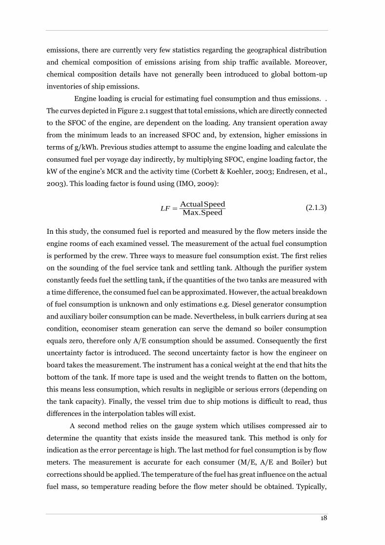
18
emissions, there are currently very few statistics regarding the geographical distribution
and chemical composition of emissions arising from ship traffic available. Moreover,
chemical composition details have not generally been introduced to global bottom-up
inventories of ship emissions.
Engine loading is crucial for estimating fuel consumption and thus emissions. .
The curves depicted in Figure 2.1 suggest that total emissions, which are directly connected
to the SFOC of the engine, are dependent on the loading. Any transient operation away
from the minimum leads to an increased SFOC and, by extension, higher emissions in
terms of g/kWh. Previous studies attempt to assume the engine loading and calculate the
consumed fuel per voyage day indirectly, by multiplying SFOC, engine loading factor, the
kW of the engine’s MCR and the activity time (Corbett & Koehler, 2003; Endresen, et al.,
2003). This loading factor is found using (IMO, 2009):
ActualSpeedMax.Speed
LF (2.1.3)
In this study, the consumed fuel is reported and measured by the flow meters inside the
engine rooms of each examined vessel. The measurement of the actual fuel consumption
is performed by the crew. Three ways to measure fuel consumption exist. The first relies
on the sounding of the fuel service tank and settling tank. Although the purifier system
constantly feeds fuel the settling tank, if the quantities of the two tanks are measured with
a time difference, the consumed fuel can be approximated. However, the actual breakdown
of fuel consumption is unknown and only estimations e.g. Diesel generator consumption
and auxiliary boiler consumption can be made. Nevertheless, in bulk carriers during at sea
condition, economiser steam generation can serve the demand so boiler consumption
equals zero, therefore only A/E consumption should be assumed. Consequently the first
uncertainty factor is introduced. The second uncertainty factor is how the engineer on
board takes the measurement. The instrument has a conical weight at the end that hits the
bottom of the tank. If more tape is used and the weight trends to flatten on the bottom,
this means less consumption, which results in negligible or serious errors (depending on
the tank capacity). Finally, the vessel trim due to ship motions is difficult to read, thus
differences in the interpolation tables will exist.
A second method relies on the gauge system which utilises compressed air to
determine the quantity that exists inside the measured tank. This method is only for
indication as the error percentage is high. The last method for fuel consumption is by flow
meters. The measurement is accurate for each consumer (M/E, A/E and Boiler) but
corrections should be applied. The temperature of the fuel has great influence on the actual
fuel mass, so temperature reading before the flow meter should be obtained. Typically,

Chapter 2
19
engineers obtain temperature measurement at the centrifugal separator or at the service
tank. Therefore uncertainty factor is again introduced. Flow meters are also sensitive to
the quality of the fuel and to the vessel trim. Based on measurements obtained during ship-
board attendances, differences between flow meter reading and soundings that exceed 4%
were observed. Nevertheless, during the sampling of the data, the fuel consumption
between fuel meters and sounding converged with very small difference which was less
than 1.4%. Thus, it is considered in this thesis that the fuel measurement is accurate
enough. Any remaining differences can be explained by sea and air inlet temperatures that
affect the performance of the engine (MAN Diesel, 2007) and the actual operation in non-
laboratory environment, which leads to an increase in the actual fuel consumption of up
to 8% of the initial, assuming the same fuel type is used.
An activity based approach is to be used later in this thesis using actual
operational data for a fleet of dry bulk vessels, together with the ‘noon reports’ of engine
performance and ‘as measured’ main engine fuel consumption, to calculate quantities of
emissions. In determining emissions, it is possible to use either a ‘power based emission
factor’ that relates emitted pollutant (g) to main engine power (kWh), or a ‘fuel based
emission factor’ relating emitted pollutant (tonnes) to daily total fuel consumption
(tonnes/day) (Psaraftis and Kontovas, 2008). These emissions factors are given in Table
2.1.
Table 2.1: Emission factors for low speed engines (TIER I) (IMO, 2009; EMEP/CORINAIR, 2002) for ‘at sea operation’. Static average power based factors and fuel based factors.
Pollutant type Static average Power based factor [g/kWh]
Fuel based factor [tonnes/day]
PM10 1.5 -
PM2.5 1.2 -
DPM 1.5 -
NOx 17 0.087
SOx 10.5 0.02*%Sulphur
CO 1.4 0.0074
HC 0.6 -
CO2 620 3.114
N2O 0.031 -
CH4 0.006 0.0003
The second IMO Greenhouse Gas study (IMO, 2009) used fuel based emission
factors, as each engine map is vessel specific. Where the operational data for the ship are
known, it is possible to account for the fluctuations in loading of the main engine from day
to day by using power based emissions factors for a broad range of loads. Although the key
to the efficiency of the proposed Hybrid Power system is in accurately assessing the effects

20
of fluctuating engine loading in SFOC, limited access to engine pollution maps make it
necessary to adopt a fuel based factor for CO2 emissions as well as NOx emissions and SOx,
since the composition of fuel is known by the bunker analysis. A reasonable modern engine
efficiency of 42% is used, without heat recovery, and judging from the correlation of SFOC
and g/kWh of pollutant gas, it can be surmised that fuel based factors take into account
engine efficiency and remain constant for ‘at sea operation’ and change at ‘at berth’ or ‘in
manoeuvring’ conditions.
An attempt to measure the implied error and the uncertainty to the calculations
by the use of a fuel based factor is presented in Table 2.2 for a modern two-stroke Diesel
Engine. It can be extracted from this table that the fluctuation of error from the engine
tuning point versus load is lower than 0.05%.
However, the fuel based factor for CO2 for this engine is significantly different to
the fuel based factor suggested by the literature and the IMO.
The means by which emissions were calculated for this study may be summarised as
follows:
CO2 emissions depend on engine efficiency, which is directly related to SFOC. The
higher the SFOC, the higher the CO2 emissions. CO2 is dependent on fuel
composition. Marine Fuels are considered to have 86.2 – 86.7 % Carbon. Hence
3.114 tonne/tonne fuel is used as an emission factor, which is within the range of
the study of Corbett & Koehler, (2003) and is adopted by the IMO (2009) for EEOI
and EEDI approximation.
SOx emissions depend on the fuel composition, which is known for each voyage,
thus the total bunker consumption (in tonnes per day) is multiplied by the
percentage of Sulphur times the emission factor.
For NOx emissions, the IMO established propulsion engine standards for Ocean
Going vessels (OGV), in Annex VI of MARPOL (2005). Engine manufacturers have
built engines to comply with that standard. Hence the limit value of 17g/kWh is
used for slow speed engines (MARPOL, 2005) which lead to a fuel based factor of
0.087 tonnes per day, which is empirical and adopted by EMEP/CORINAIR
(2002).
Ageing of engines, poor maintenance and actual operation in non-ISO conditions
result in a decrease of engine efficiency and an increase of the SFOC. Consequently the ‘as
measured’ fuel consumption will still imply a degree of uncertainty for the NOx emissions,
although the real engine is likely to emit more than what is assumed in this study.

Chapter 2
21
Table 2.2: Comparison and calculation of implied error of fuel based factors and power based factors for a Marine Diesel Engine of K98MC-C Tier II
Load SFOC Difference%
CO2 Fuel
Factor
Difference %
SOx NOx
1.00 170.5 2.3 559 3.279 0.039 11.94 0.07003
0.059
13.5 0.079
-10.264
0.90 168.4 1.1 552 3.278 0.018 11.79 0.07001
0.034
14.2 0.0843
-4.434
0.80 167 0.2 547 3.275 -0.057 11.69 0.07000
0.017
14.6 0.0874
-0.918
0.75 166.7 0.1 546 3.275 -
0.060 11.67
0.07001
0.026
14.7 0.0882
-0.060
0.70 166.6 546 3.277 11.66 0.06999
14.7 0.0882
0.65 167 0.2 547 3.275 -0.057 11.69 0.07000
0.017
14.7 0.0880
-0.240
0.60 167.8 0.7 550 3.278 0.012 11.75 0.07002
0.051
14.6 0.0870
-1.391
0.55 168.8 1.3 553 3.276 -0.038 11.82 0.07002
0.051
14.5 0.0859
-2.646
0.50 170 2.0 557 3.276 -0.026 11.9 0.07000
0.017
14.5 0.0853
-3.333
0.45 171.4 2.9 562 3.279 0.047
9 12
0.07001
0.034
14.4 0.0840
-4.784
0.35 174.6 4.8 572 3.276 -0.038 12.2
2 0.06999
0.001
14.4 0.082
5 -6.529
In order to evaluate the effectiveness with the static power based factor and the
fuel based factor, a set of voyages in laden and ballast was evaluated using both types of
factors. Table 2.3 describes the operational routes examined for this study.

22
Table 2.3: Examined set of voyages for emission factor evaluation
Vessel Departure port Arrival port Travelled distance
Quantity (MT)
Vessel condition
PPVSL 1 Rio Grande Marin 5168 60600 Laden
Hong Kong Tubarao 9435 39063 Ballast
PPVSL 2 Tubarao Amsterdam 5045 80000 Laden
Port Talbot Port Cartier 2610 39060 Ballast
PPVSL 3 Dalrymple Bay Taranto 9535 89524 Laden
Luoyan Dalrymple bay 3906 39121 Ballast
Emission calculations are performed for each voyage and for every vessel. As an outcome,
emissions per tonne mile can be calculated by dividing the emitted tonnes by the cargo
capacity and travelled miles (Psaraftis and Kontovas, 2008). Figures 2.2, 2.3 and 2.4 show
the gasses emitted during the voyages, and a comparison of emission studies and factors
is performed.
Figure 2.2: Comparison of ‘Activity’ method of power based factors (PBF) and fuel based factors (FBF) with LMT assumptions, for CO2 emissions
0
2
4
6
8
10
12
14
PBFLDN FBFLDN PBFBLS FBFBLS
C0
2 E
mis
sio
ns
[ g
/to
n*m
iles
] PPVSL1 PPVSL2 PPVLS3

Chapter 2
23
Figure 2.3: Comparison of ‘Activity’ method of power based factors (PBF) and fuel based factors (FBF) with LMT assumptions, for SOx emissions
The calculation of emissions showed differences between fuel based and power
based emission factors. This deviation, along with the general assumption of ship
operation, introduces uncertainty and, as can be seen in the comparison graphs, it
overestimates emissions such as CO2 and underestimates NOx. However, in cases where
daily reports do not exist, the rough assumptions of engine loading and vessel speed can
represent voyage emissions with acceptable accuracy.
Figure 2.4: Comparison of ‘Activity’ method of power based factors (PBF) and fuel based factors (FBF) with LMT assumptions, for NOx emissions
0.0
0.1
0.1
0.2
0.2
0.3
PBFLDN FBFLDN PBFBLS FBFBLS
SO
x E
mis
sio
ns
[g/t
on
*mil
es]
PPVSL1 PPVSL2 PPVLS3
0.0
0.1
0.1
0.2
0.2
0.3
0.3
0.4
PBFLDN FBFLDN PBFBLS FBFBLS
NO
x E
mis
sio
ns
[g/t
on
*mil
es]
PPVSL1 PPVSL2 PPVLS3

24
IMO through the adoption of the MEPC62 and resolution 203 had officially linked
shipping emissions with vessel energy efficiency. For this reason, the IMO adopted a set of
formulae that attempt to estimate the vessels’ environmental impact and in more detail,
their carbon footprint. The latter formulae relate the installed power to the energy
efficiency index, taking into account the auxiliary engines, the specific fuel consumption
curves, the existence of heat recovery systems and push and pull systems that reduce the
propulsive energy (e.g. kites, sails etc.) and innovative sustainable energy devices, such as
wind turbines and photovoltaic systems. In addition, they consider the vessel’s design
speed and the Deadweight and correction factors for sea-vessel interaction and for Ice
Class ships. However, many scientific objections have been raised during last 5 years IMO
MEPC meetings with regards to the EEDI reduction, benchmarking, specific vessel types
applicability, contribution factors of hydrodynamic energy saving devices and the
reduction factors for large vessels and the and applicability dates. Nonetheless, problems
arise when the emission policy and the measures to improve the EEDI are taken into
account. The main problem identified in this formula is measrues in order to decrease the
EEDI, and thus reduce the environmental impact, serious concerns raised for
underpowered ships, with implications on safety and manoeuvrability, weather margin
performance and easy solution to reduce speed instead of optimise the hull forms. In
addition, the shipyards shift towards increasing the DWT, maintaining the same
displacement and reducing the lightweight, which results in a potential decrease of the
vessel’s lifecycle, rasing concerns about the structural ability. During MEPC 62 meeting
Greece opposed to Japan regarding the structural enchacements that proposed in order to
tackle the structural concerns, convincing the committee that structural safety cannot be
compromised.
The formula of EEDI is given by the equation (2.1.4). It can be identified from the
formula (2.1.4) that the fuel type expressed with the coefficient CF inserts the emission
factor into the EEDI formula. The rest combine the vessel’s energy efficiency with the
emissions at the design stage. This formula is due to be updated in order to take into
account the Diesel Electric installations and the Hybrid Power systems.
/
/ /
/
/
/ /
11
/
/ / /
1 1
/
1
M E
A E A E
M E
m nM E
ci F M E M E
ij
nM E nWHR
A E F A E PTI WHR F A E
i i
reff
eff eff F M E
i
j ref w
f C SFOC P
P C SFOC P P C SFOC
f P C SFOC
EEDIf DWT V f
(2.1.4)

Chapter 2
25
where,
fci : Correction factor to account ship specific design elements [-]
CF M/E : M/E fuel carbon content [-]
SFOCM/E : M/E specific fuel oil consumption [g/kWh]
PM/E : M/E power output [kW]
CF A/E : A/E fuel carbon content [-]
SFOCA/E : A/E specific fuel oil consumption [g/kWh]
PA/E : A/E power output [kW]
PPTI : Power take off (PTI) power output [kW]
PWHR : Waste heat recovery (WHR) equivalent power output [kW]
DWT : Vessels deadweight [tonnes]
feff : Availability factor of innovative energy saving technology [-]
Peff : 75% of the M/E power reduction due to application of innovative
technology [kW]
Vref : Vessel desing/ reference speed [knots]
fw : Non-dimentional coefficient indicating decrease due to environmental
condtions [-]
fj : Capacity factor for any technical/regulatory limitation on capacity [-]
Unfortunately, the modern regulations regarding the Nitrogen Oxides, insert a
penalty parameter to the EEDI calculation. In terms of grammes of specific pollutant per
kWh, a trade-off between NOx and SFOC exists. The first marine slow speed Diesel engines
meeting Tier II requirements (NOx less than 14.4g/kwh) in order to reduce the amount of
these oxides, decreased the combustion pressure. This method directly affected the engine
fuel efficiency and thus, the SFOC increased by up to 6g/kWh for camshaft controlled
engines and by 4g/kWh for the electronically controlled engines (MAN Diesel, 2009b).
The observed difference between the electronic and camshaft engines is explained by the
existence of better control of valve timing, injection parameters (rate shaping) and finally
due to design improvements as the electronic engines are newer compared to the camshaft
ones. Nonetheless, in order to meet the nitrogen oxides limits, modifications on the
combustion process are implemented. The introduction of lower combustion temperatures
despite the NOx reduction, the SFOC is increased. In addition, a very promising technology
of exhaust gas recirculation (EGR) which reduces the oxygen content inside the cylinder
during scavenging process also reduces fuel efficiency. Furthermore, the application of
two-stage turbocharging inserts a fuel penalty which is less than the previous depicted
values and is considered as a very promising technology as well. In addition, the water in
fuel technology (WIF) may increase SFOC (in TIER II engines) by up to 5% at the 75%
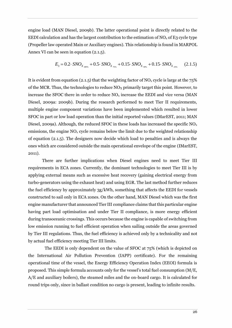
26
engine load (MAN Diesel, 2009b). The latter operational point is directly related to the
EEDI calculation and has the largest contribution to the estimation of NOx of E3 cycle type
(Propeller law operated Main or Auxiliary engines). This relationship is found in MARPOL
Annex VI can be seen in equation (2.1.5).
100% 75% 50% 25%3 0.2 0.5 0.15 0.15X X X XE SNO SNO SNO SNO (2.1.5)
It is evident from equation (2.1.5) that the weighting factor of NOx cycle is large at the 75%
of the MCR. Thus, the technologies to reduce NOX primarily target this point. However, to
increase the SFOC there in order to reduce NOx increase the EEDI and vice versa (MAN
Diesel, 2009a: 2009b). During the research performed to meet Tier II requirements,
multiple engine component variations have been implemented which resulted in lower
SFOC in part or low load operation than the initial reported values (IMarEST, 2011; MAN
Diesel, 2009a). Although, the reduced SFOC in these loads has increased the specific NOx
emissions, the engine NOx cycle remains below the limit due to the weighted relationship
of equation (2.1.5). The designers now decide which load to penalties and is always the
ones which are considered outside the main operational envelope of the engine (IMarEST,
2011).
There are further implications when Diesel engines need to meet Tier III
requirements in ECA zones. Currently, the dominant technologies to meet Tier III is by
applying external means such as excessive heat recovery (gaining electrical energy from
turbo-generators using the exhaust heat) and using EGR. The last method further reduces
the fuel efficiency by approximately 3g/kWh, something that affects the EEDI for vessels
constructed to sail only in ECA zones. On the other hand, MAN Diesel which was the first
engine manufacturer that announced Tier III compliance claims that this particular engine
having part load optimisation and under Tier II compliance, is more energy efficient
during transoceanic crossings. This occurs because the engine is capable of switching from
low emission running to fuel efficient operation when sailing outside the areas governed
by Tier III regulations. Thus, the fuel efficiency is achieved only by a technicality and not
by actual fuel efficiency meeting Tier III limits.
The EEDI is only dependent on the value of SFOC at 75% (which is depicted on
the International Air Pollution Prevention (IAPP) certificate). For the remaining
operational time of the vessel, the Energy Efficiency Operation Index (EEOI) formula is
proposed. This simple formula accounts only for the vessel’s total fuel consumption (M/E,
A/E and auxiliary boilers), the steamed miles and the on-board cargo. It is calculated for
round trips only, since in ballast condition no cargo is present, leading to infinite results.
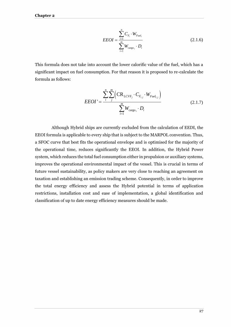
Chapter 2
27
1
cargo
1
i i
i
n
F Fuel
i
m
i
i
C W
EEOI
W D
(2.1.6)
This formula does not take into account the lower calorific value of the fuel, which has a
significant impact on fuel consumption. For that reason it is proposed to re-calculate the
formula as follows:
, ,LCVF
cargo1
CR
'i jj i j
i
n m
F Fueli j
m
ii
C W
EEOI
W D
(2.1.7)
Although Hybrid ships are currently excluded from the calculation of EEDI, the
EEOI formula is applicable to every ship that is subject to the MARPOL convention. Thus,
a SFOC curve that best fits the operational envelope and is optimised for the majority of
the operational time, reduces significantly the EEOI. In addition, the Hybrid Power
system, which reduces the total fuel consumption either in propulsion or auxiliary systems,
improves the operational environmental impact of the vessel. This is crucial in terms of
future vessel sustainability, as policy makers are very close to reaching an agreement on
taxation and establishing an emission trading scheme. Consequently, in order to improve
the total energy efficiency and assess the Hybrid potential in terms of application
restrictions, installation cost and ease of implementation, a global identification and
classification of up to date energy efficiency measures should be made.

28
2.3 Improving the energy efficiency of the vessels
The term ‘system efficiency’ refers to the ability of the energy system to have its output as
close as possible to its input, minimising the losses. For the vessel, the energy efficiency
targets the propulsion system, whose input is the fuel (whether it is petroleum or LNG)
and its output the propulsive power (thrust) and electricity for auxiliary loads. Energy
efficiency is making the best possible use of the energy expended to obtain the maximum
work done in order to achieve fuel savings. Energy efficiency increases either when the
energy input is reduced for a given level of service, or when services are increased and
enhanced for a given amount of energy input. Proposed ways of increasing fuel efficiency
can be broken down into four categories, depending on their targeting area, as follows:
Thus,
Improving vessel operations
Improving the ship’s total resistance
Improving propulsion (hydrodynamic side)
Improving power generation and on-board consumption
With the aim of enhancing ship energy efficiency, the baseline vessel has to be
defined. The baseline vessel is an ideal vessel, which is hydro-dynamically highly
optimised, the coupling of propeller and engine is ideal, and the superstructure design
secures minimum air-drag. This explains the fact that many energy saving devices have
valid savings for initially bad designs, where the aforementioned hydrodynamic vessels
never can reach the claims made about them (VLCC workgroup, 2009). In terms of
machinery efficiency, the vessel is equipped with state of the art technologies, and external
abatement techniques for NOx and SOx reduction are installed. The energy saving devices
that will be presented below do not increase the baseline vessel dramatically. Nevertheless,
as it was stated earlier, modern vessels are DWT optimised and their reference line is well
below the baseline vessel. As a result, the saving potentials should not be summed up and,
of course, the outcome will not lead to an energy independent ship. In order to improve
energy efficiency resulting in the reduction of the power requirement, two categories of
measures/practices have been identified.
Operational practices target ship operations and management. These practices
aim to improve the energy efficiency with zero investment cost. Their implementation
ranges from easy adoption to very hard/impossible implementation by the crew or
impossible for the examined ship type due to constraint parameters, such as the ship
safety, operational restrictions by ports and/or charterers, etc.

Chapter 2
29
Technical measures target vessel retrofitting and installation of energy saving
devices. This category includes the hydrodynamic improvement devices and machinery
optimisation and retrofitting. Usually, these practices have a notable cost and their
selection should be made in accordance with a detailed financial calculation. The
implementation period is during dry-docking, and the crew’s working environment and
procedures after the implementation of these measures is not significantly affected.
In order to evaluate the effectiveness of the adopted measures and practices,
performance monitoring tools should be installed on-board. Performance monitoring is
usually executed by specific electronic software and hardware sensors. The results are
transmitted to the managing company for evaluation. In the event that there are
indications of vessel performance deterioration, the company can take immediate action
within a very short response time, thus ensuring that energy efficiency would remain high.
2.4 Operational and port methods to reduce emissions
‘Slow steaming’ is a term used to describe the method of decreasing the average vessel
sailing speed. The range of operational speeds is determined by the charterers and is
related to the shipping business. When speed is reduced, engine loading decreases by a
cubic relationship, thus the total amount of fuel burnt is significantly lower. However, in
terms of specific fuel oil consumption, slow steaming reduces fuel efficiency. Moreover,
carbon emissions are connected to fuel consumption only. Hence, carbon emissions are a
new parameter in the shipping transportation system. Corbett et al. (2009) and Cariou
(2011) have demonstrated that slow steaming is applicable to container vessels that are
high-speed ships and hence the installed power is high. They have shown that, although it
may require more ships (Psaraftis and Kontovas, 2009; 2010), slow steaming in
containerships has so far led to an 11% decrease of CO2 emissions.
Pollution in ocean going ships is important, however, significant pollution occurs
in high traffic ports. In-port emissions make up a small percentage of the overall emissions
from shipping (Whall et al., 2002; Dalsøren et al., 2009); ports attract shipping traffic and
inevitably constitute points of concentrated ship exhaust emissions. The unified port of
San Diego in the United States has employed Starcrest Consulting (2006) to apply a
bottom-up approach to estimate emissions from all port operations. Furthermore,
Tzannatos (2010) underlines the importance of Piraeus’ harbour shipping operations in
emission percentages, which significantly downgrade the air quality around the harbour
and affect human health. Furthermore, the impact of Los Angeles port on air quality is
discussed in Ault et al. (2009). The examined studies conclude that emission factors are
not accurate for in-port emission estimation, and detailed pollution engine maps are

30
required. Nevertheless, the total amount of local CO2, NOx, SOx and particulate matter
emissions is noteworthy and cannot be excluded from emission inventories.
Following the importance of local ship emissions, technology considerations and
available ways to plug ships with shore power, a method commonly known as ‘cold
ironing’, are presented in Khersonsky et al. (2007). This feature makes it possible to cease
utilising generator engines that burn fuel inside the harbours, making the ship operation
carbon free. However, Hall (2010) demonstrated that shore power leads to a decrease in
emissions only when electricity from the grid is produced and transferred more efficiently
than the power that ships can generate themselves. However, in terms of local emissions
in every port, significant reductions are possible.
Weather Routing is the optimisation of a ship’s course and speed that may reduce
the average added resistance in seaways. IMO (2009) state that fuel savings can be as high
as 5%. However, some experts estimate the saving potential to lower than 1% for more
realistic scenarios. Weather routing should be combined with the tactic of slow steaming
or optimised voyage control, and just in time arrival (JIT). Optimum voyage control refers
to the optimum route, and improved efficiency can be achieved through the careful
planning and execution of the voyages, reducing the total voyage miles, hence fuel
consumption. JIT is a voluntary speed reduction upon agreement with the charterers to
reduce speed and thus the total fuel consumption, because of known delays at the next
port. This approach increases the time spent in laden or ballast and reduces the time spent
in anchorage or alongside.
Based on hydrodynamic performance, the trim is a significant parameter in a
vessel’s fuel consumption. IMO (2009) INTERTANKO and INTERCARGO underline the
importance of the trim and encourage crew performing trials in order to identify the trim
that leads to the lowest fuel consumption under specific weather conditions.
Pumps and fans should be operated according the electric load analysis provided
by the Yard. The crew should use port cooling pumps at port or anchorage, when available.
This minimises the fuel consumption of auxiliaries. Cooling/ventilation systems are not
always under full load/RPM. Installation of a speed/power control unit for engine room
pumps and fans will conserve electrical energy demand, where pumps are not required to
operate at their full-speed rating.
The cargo/voyage-specific heating requirements and the Charterer/Cargo
Receiver requirements should be taken into account when carrying crude oil. Excessive
use of auxiliary boilers leads to significant fuel costs, and managing companies have
established that optimised cargo heating may reduce Auxiliary Boiler consumption by up
to 20%. In addition to the above, it is proposed to perform optimum lighting management
and to promote smart lighting controllers, by turning off all unnecessary lights. Moreover,
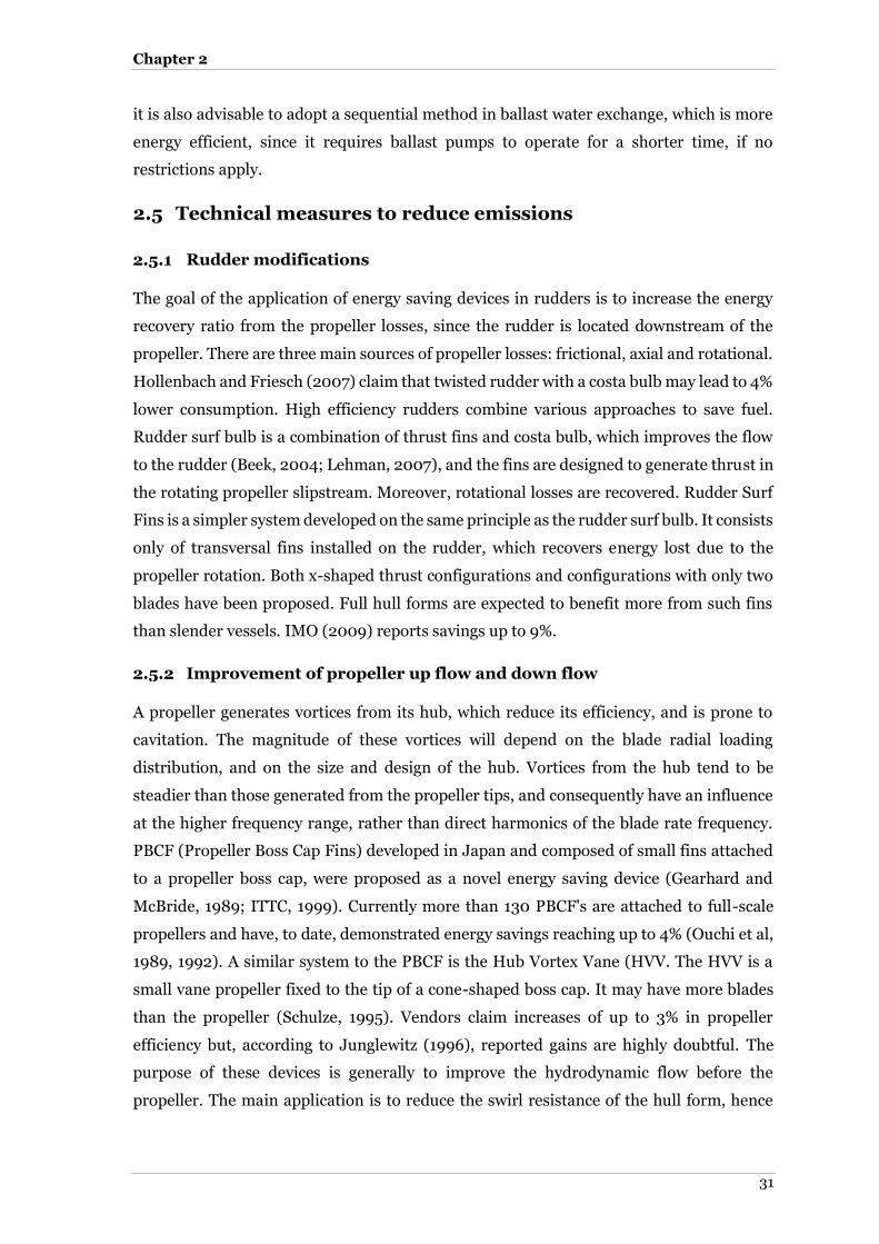
Chapter 2
31
it is also advisable to adopt a sequential method in ballast water exchange, which is more
energy efficient, since it requires ballast pumps to operate for a shorter time, if no
restrictions apply.
2.5 Technical measures to reduce emissions
Rudder modifications
The goal of the application of energy saving devices in rudders is to increase the energy
recovery ratio from the propeller losses, since the rudder is located downstream of the
propeller. There are three main sources of propeller losses: frictional, axial and rotational.
Hollenbach and Friesch (2007) claim that twisted rudder with a costa bulb may lead to 4%
lower consumption. High efficiency rudders combine various approaches to save fuel.
Rudder surf bulb is a combination of thrust fins and costa bulb, which improves the flow
to the rudder (Beek, 2004; Lehman, 2007), and the fins are designed to generate thrust in
the rotating propeller slipstream. Moreover, rotational losses are recovered. Rudder Surf
Fins is a simpler system developed on the same principle as the rudder surf bulb. It consists
only of transversal fins installed on the rudder, which recovers energy lost due to the
propeller rotation. Both x-shaped thrust configurations and configurations with only two
blades have been proposed. Full hull forms are expected to benefit more from such fins
than slender vessels. IMO (2009) reports savings up to 9%.
Improvement of propeller up flow and down flow
A propeller generates vortices from its hub, which reduce its efficiency, and is prone to
cavitation. The magnitude of these vortices will depend on the blade radial loading
distribution, and on the size and design of the hub. Vortices from the hub tend to be
steadier than those generated from the propeller tips, and consequently have an influence
at the higher frequency range, rather than direct harmonics of the blade rate frequency.
PBCF (Propeller Boss Cap Fins) developed in Japan and composed of small fins attached
to a propeller boss cap, were proposed as a novel energy saving device (Gearhard and
McBride, 1989; ITTC, 1999). Currently more than 130 PBCF's are attached to full-scale
propellers and have, to date, demonstrated energy savings reaching up to 4% (Ouchi et al,
1989, 1992). A similar system to the PBCF is the Hub Vortex Vane (HVV. The HVV is a
small vane propeller fixed to the tip of a cone-shaped boss cap. It may have more blades
than the propeller (Schulze, 1995). Vendors claim increases of up to 3% in propeller
efficiency but, according to Junglewitz (1996), reported gains are highly doubtful. The
purpose of these devices is generally to improve the hydrodynamic flow before the
propeller. The main application is to reduce the swirl resistance of the hull form, hence

32
reducing the viscous pressure resistance. Devices aiming to fix the flow to the propeller are
the Sanoyas Tandem Fins, the IHI low Viscous Resistance Fins, the Grotheus Spoilers, the
Oshima Wake Acceleration Fin and the Namura flow Control Fin. Although these vortex
generators have been employed to fix design flaws leading to vibration, it is expected that
they increase fuel consumption rather than lead to any fuel savings.
The purpose of the Pre-swirl Stator system is to produce a swirling flow opposed
to the direction of rotation of the propeller, thereby annulling the swirl induced by the
propeller and, at the same time, increasing the relative tangential velocity of the propeller
blades. Thus, propulsive efficiency is increased and the cavitation of the propeller is
reduced (Linjenberg, 2006).
The Mewis Duct is a novel power saving device which has been developed for
slower ships with full form hull shape, that allows either a significant fuel saving at a given
speed or alternatively for the vessel to travel faster for a given power level. The duct
diameter is smaller than the propeller diameter and the fins chord length only covers part
of the duct’s length. The MD combines the effects of a wake equalizing duct and pre-swirl
fins within a single unit. By pre-correcting the flow into the propeller, the device essentially
reduces the rotational losses and increases the flow velocity towards the inner radii of the
propeller (Hollenbach and Reinholz, 2011). The pre swirl is claimed to reduce rotational
losses and also to contribute to a reduction of energy loss due to generation of hub vorticity.
The achievable power savings from the Mewis Duct are strongly dependent on the
propeller thrust loading, ranging from 3% for small multi-purpose ships to up to 9% for
large tankers and bulk carriers. HSVA denotes that the power saving is about 6.0% at 16
knots sailing speed, which corresponds to a speed increase of 0.27 knots (Hollenbach and
Reinholz, 2011). Ouchi (1989) states that the power saving is virtually independent of ship
draught and speed. The Mewis Duct is ideally suited to both new-builds and retrofit
applications. There are two types of duct that are applicable to marine propellers. The first
type is called accelerating Duct and the second decelerating. The proprietary brand of
accelerating propeller is the Kort nozzle. Attention should be paid to the fact that the
efficiency of ducted propellers when free-running and lightly loaded tends to be less than
that of a non-ducted propeller, because of the additional shrouding which adds drag,
resulting in the Kort nozzles losing their advantage at around 10 knots. Ducted propellers
have been around for many decades and very few ships, mainly tankers, were fitted in the
1970s. The practice was abandoned reportedly due to problems with vibration and
cavitation. According to IMO (2009), potential savings can be as high as 20%.
The wake behind single-screw ships is non-homogenous (i.e. there are very low velocities
at the top of the propeller disc). This induces pressure fluctuations on the propeller and
the ship hull above the propeller, which in turn excite vibrations. The magnitude of these

Chapter 2
33
vibrations poses more or less restrictive constraints on the propeller design. It is assumed
that improving the homogeneity of the wake will improve propulsion efficiency (the results
mainly affect open water propeller efficiency). Optimising the angle of the partial duct to
the stern under load conditions is said to improve the homogeneity of the wake. Wake
equalising devices, such as Schneeklith nozzles (or Wake Equalising Ducts (WED))
(Schneekluth, 1986; Schneekluth and Bertram, 1998), the Sumitomo integrated
Lammeren Duct (SILD) or the Hitachi Zosen Nozzle, may improve propulsion.
Nonetheless, independent analyses result in contradicting evaluations of the effectiveness
of WEDs (Celik (2007; ITTC, 1999).
The above technologies may increase propeller performance, leading to higher
fuel efficiency because of the reduction in required torque. Reduction in friction resistance,
by means of advanced painting or regular cleaning, or by using novel systems, such as air
lubrication, should also be considered. In addition, wave added resistance plays a
significant part in bad weather, or when sailing at high speeds.
Minimisation of ship total resistance
Coatings may effectively reduce frictional resistance. Silicon based antifouling is a new
generation of paints that employ a Foul Release mechanism. ‘Foul release’ is the name
given to the technology that does not use biocides to control fouling, but provides an ultra-
smooth, slippery, low friction, hydrophobic or hydrophobic/hydrophilic combination
surface, onto which fouling organisms have difficulty in settling. The available Foul
Release products contain no added biocides and are based on silicone/fluoro-polymer
technology. Some publications claim improvements in excess of 10%. However, this is
partially true after dry-docking. Over longer periods, this notable effect fades out.
Routine in-service polishing of the propeller reduces its surface roughness caused by
organic growth and fouling. There is evidence that the effects of a poorly maintained
propeller can decrease speed and fuel efficiency by up to 3% compared to that of a propeller
maintaining an ‘A’ finish on the Rupert Scale.
Hull cleaning should be carried out on a condition assessment basis, as the
increased roughness significantly increases the friction resistance. Therefore, in
conjunction with every propeller polishing, the hull should be inspected for damage and
marine growth. If there is significant growth on the hull, an immediate decision to clean
the hull could be made by the Company, taking into account the report/notification by the
Master.
The main components of ship resistance consist of resistance due to wave drag, pressure
drag, and frictional drag. A promising alternative technique to obtain lower frictional
resistance is to use air as a lubricant in order to reduce the wetted surface of the ship. Three

34
distinct approaches are identified: the injection of bubbles, air films, and air cavity ships
(Foeth et al., 2008; Ceccio, 2010).
Hirota et al. (2004), based on model test results, state that the sharpness of the
bow shape above the calm waterline could reduce added resistance. With a blunter bow
shape, such as that of tankers or bulk carriers, waves are mostly reflected forward and so
the resistance increases. The increase in wave resistance acting on such full-form ships
with a blunt bow is therefore larger than that on slender ships. For blunt-bow shaped full-
form ships with a smaller power engine, the speed loss is estimated to be larger than that
for ships with a conventional high power engine. To improve the performance in waves for
ships with a low power engine, the resistance increase in waves needs to be reduced. To
achieve this, the bow should be made less blunt. Results of a study on the effect of bow
bluntness on the resistance increase indicated that the most effective way was to sharpen
the bow shape above the still water level, where the wave surface is elevated and reflected.
By sharpening this part, the incident wave is reflected mostly to the side, not forwards,
thus reducing the wave resistance acting backward. Ax-Bow design may reduce the
resistance increase in waves by 20% to 30% in almost the entire range of wavelength. This
enables a 4 to 6% reduction of horsepower, or fuel consumption, in the case of sea
conditions corresponding to a 20% sea margin. This new bow shape has been applied to
ships already and, according to NKK (2002), trials showed that the Ax-bow indeed leads
to reduced speed loss in waves.
Wind assisted concepts predominantly use other means of power (typically Diesel
Engines), and wind power plays a secondary role to the propulsion. Generally, these
systems may be attractive for slow speed vessels (< 15 knots). For modem vessels, the only
viable solution for wind assisted propulsion is for fully automated systems. Moreover,
additional structural effort for mast support on the ships with sails can be considerable.
Kites and Flettner rotors are generally more efficient than sails per surface area. Optimum
solutions depend on the operational profile of the vessel and the type of vessel. Schenzle
(2010) analysed various advanced sail-assistance options for a Panamax Bulk Carrier.

Chapter 2
35
Improvements in the propulsion machinery
De-rating is one of the available options to reduce the specific fuel oil consumption of
Diesel engines. It is also known as ‘economy’ rating. This means that the operation of the
engines takes advantage of the maximum cylinder pressure for the design continuous
service rating (CSR), while the mean effective pressure and shaft speed is lower, at an
operational point lower of the propeller normal operating curve. Fuel efficiency is
improved when the ratio of Mean Effective pressure and the maximum pressure is
increased (Woodyard, 2009). In combination with de-rating and in order to uncouple the
injectors and the valve timing with the rotational speed of the engine through a camshaft
(camshaft controlled engines), the installation of electronically controlled M/E is
proposed. The main purpose of switching to electronic control is to ensure fuel injection
timing and rate, as well as exhaust valve timing and operation, exactly when and as desired
according to the engine load. As a result, fuel injection, exhaust valve actuating and
starting air systems are controlled electronically and are optimised for all operation loads.
NOx emission can be reduced and smokeless operation can be achieved (Woodyard,
2009).
Although the operation of the engine can be controlled either by the camshaft or
by electronic control systems, the engine speed is crucial in terms of fuel efficiency.
Nowadays it is proposed to install an electronic governor instead of its mechanical
counterpart. The purpose of the governor is to regulate the amount of fuel supplied to the
cylinders so that a predetermined engine speed will be maintained despite variations in
load. Based on ship-board measurements for the purpose of this study, it was found that
fuel savings can be as high as 9% per day in laden condition and 7.5% per day in ballast
condition.
Despite the efforts to improve fuel efficiency at low loads using electronic control,
more radical solutions are needed, especially when vessels are designed to operate at full
load, but the volatile state of the market has forced the shipping companies to operate the
vessels at very low loads. The Turbocharger Cut-out system is designed to lower the fuel
oil consumption and improve the main engine performance during part-load operation by
isolating one, two or three turbochargers, depending on the total number installed.
Another measure to increase the fuel efficiency of a Marine Diesel engine in low
loads is the introduction of the Cylinder cut-out system. The cylinder cut-out system
should be used at RPM below 40% of MCR RPM, allowing the engine to operate with only
half of the cylinders, resulting in increased load on the operating cylinders with improved
operating conditions for the fuel system. As a result, it ensures stable running conditions
down to 20-25% of the nominal RPM.

36
A potential solution to reduce PM and NOx emissions are slide fuel valves. The
latter have also shown significant savings, lower emissions and lower fuel consumption.
The slide fuel valves both optimise the combustion of the fuel and ensure a cleaner engine.
The spray pattern of the fuel is further optimised and therefore leads to an improved
combustion process (Woodyard, 2009).
However, not every measure can be retrofitted to the existing vessels, nor be
applied in combination with others. The following Table 2.4 presents the compatibility of
each hydrodynamic device with each other for potential combination of these technologies
(Carlton, 2008).
Table 2.4: Compatibility of hydrodynamic devices amended from Carlton (2008) and based on previous work by the author performed during training for new-building projects in
shipping company
Compatibility of Technologies C- Fully Compatible N - No
compatibility PC- Partly Compatible
Mew
is D
uct
Pro
pel
ler
Bo
ss C
ap
Fin
s P
re S
wir
l Sta
tor
Pro
pel
ler
No
zzle
Co
ntr
a R
ota
tin
g
Pro
pel
ler
Pro
pel
ler
Ru
dd
er
tran
siti
on
bu
lb
Ru
dd
er P
rofi
le
Wak
e Eq
ual
isin
g
Du
ct
Pro
pel
lers
wit
h
end
-pla
tes
Gri
m v
an w
hee
l
Ru
dd
er b
ulb
fin
s
Ad
dit
ion
al t
hru
st
fin
s
Mewis Duct PC N N N PC C N N N N N
Propeller Boss Cap Fins P C N C C N PC N N C
Pre Swirl Stator PC N PC C N C N C C
Propeller Nozzle N C C N C N N PC
Contra Rotating Propeller
N C N N N N N
Propeller Rudder transition bulb
C N PC N N C
Rudder Profile
C C C C C
Wake Equalising Duct C N N N
Propellers with end-plates C N N
Grim van wheel
N N
Rudder bulb fins
N
Additional thrust fins
Furthermore, a classification attempt of the operational and technical measures
is attempted with respect to implementation ease, initial cost and whether or not the
selected measure is appropriate for retrofitting. The results are presented in Table 2.5 and
Table 2.6. The classification of Energy saving practices and measures in terms of cost is
considered as:
‘Low’ when the annual corresponding amount is between 1 $ and 50,000 $
‘Medium’ when the annual corresponding amount is over 50,000 $ and less than
100,000$
‘High’ when the annual corresponding amount is over 100,000 $
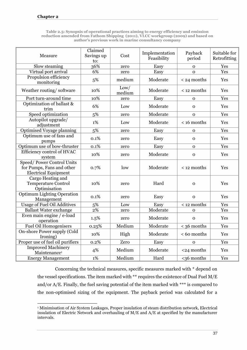
Chapter 2
37
Table 2.5: Synopsis of operational practices aiming to energy efficiency and emission reduction amended from Fathom Shipping (2011), VLCC workgroup (2009) and based on
author’s previous work in marine consultancy company
Measure Claimed
Savings up to:
Cost Implementation
Feasibility Payback period
Suitable for Retrofitting
Slow steaming 36% zero Easy 0 Yes Virtual port arrival 6% zero Easy 0 Yes
Propulsion efficiency monitoring
5% medium Moderate < 24 months Yes
Weather routing/ software 10% Low/
medium Moderate < 12 months Yes
Port turn-around time 10% zero Easy 0 Yes Optimization of ballast &
trim 6% Low Moderate 0 Yes
Speed optimization 5% zero Moderate 0 Yes Autopilot upgrade/
adjustment 1% Low Moderate < 16 months Yes
Optimised Voyage planning 5% zero Easy 0 Yes Optimum use of fans and
pumps 0.1% zero Easy 0 Yes
Optimum use of bow-thruster 0.1% zero Easy 0 Yes Efficiency control of HVAC
system 10% zero Moderate 0 Yes
Speed/ Power Control Units for Pumps, Fans and other
Electrical Equipment 0.7% low Moderate < 12 months Yes
Cargo Heating and Temperature Control
Optimisation 10% zero Hard 0 Yes
Optimum Lighting Operation Management
0.1% zero Easy 0 Yes
Usage of Fuel Oil Additives 5% Low Easy < 12 months Yes Ballast Water exchange 2% zero Moderate 0 Yes
Even main engine / e-load operation
1.5% zero Moderate 0 Yes
Fuel Oil Homogenisers 0.25% Medium Moderate < 36 months Yes On-shore Power supply (Cold
Ironing) 10% High Moderate < 60 months Yes
Proper use of fuel oil purifiers 0.2% Zero Easy 0 Yes Improved Machinery
Maintenance1 4% Medium Moderate <24 months Yes
Energy Management 1% Medium Hard <36 months Yes
Concerning the technical measures, specific measures marked with * depend on
the vessel specifications. The item marked with ** requires the existence of Dual Fuel M/E
and/or A/E. Finally, the fuel saving potential of the item marked with *** is compared to
the non-optimised sizing of the equipment. The payback period was calculated for a
1 Minimisation of Air System Leakages, Proper insulation of steam distribution network, Electrical insulation of Electric Network and overhauling of M/E and A/E at specified by the manufacturer intervals.

38
baseline VLCC vessel with expected operational life of more than 25 years. Furthermore,
savings should be added by multiplying the reduced power consumption. With this
method, the implied error in the case of simple addition is negligible (VLCC workgroup,
2009).
The adoption of energy efficiency measures leads to a total reduction of fuel oil
consumption under favourable conditions for each measure. However, the operational
practices and hull modification target is to decrease the energy demand and not to improve
the production of energy, which leads to the fuel efficiency. For the practices and measures
that minimize the demand, the proposed Hybrid Power system is suitable for installation
as it is aimed at improving the energy production.
When the installed machinery comprises of Diesel Engines, the Hybrid Power
topologies aim to increase the thermodynamic efficiency of the prime movers for the given
operational scenario. However, it must be taken into account that the cost of Hybrid
machinery is considered high, as will be shown in Chapter 3, and the outcome of the
Hybrid Power system might be compensated by cheaper solutions of the current market.
This statement is valid only when the vessel is designed for a specific purpose.
This means that when the ship is designed for ultra-slow steaming, then a better engine
propeller match will be performed at the early design stages and the fuel efficiency will be
tuned by the manufacturer in order to serve the specific operational scenario. The hybrid
system is not recommended for these cases. Nonetheless, when the vessel is designed for
a broad operational range, as the entire fleet that was examined in this study, energy saving
potentials such as turbocharger cut-out, cylinder isolation or engine de-rating maybe
proved very hard or even impossible to implement during specific voyages, as they require
dry-docking or modification to be performed by a special service team dispatched by the
engine manufacturer. Consequently, the Hybrid potential is attractive in terms of real time
applicability. Moreover, due to the optimisation of the Hybrid power plant and the
existence of the proposed smart Hybrid controller, the engine operation may not be
affected if the solution yields to a zero hybridisation degree. Thus, the existence of the
hybrid system on-board does not affect other energy saving measures of the propulsion
machinery while they are in place.
Therefore, it can be concluded that the Hybrid Power system is suitable in
combination with many energy saving options, and is fully compatible with operational
practises, although saving percentages are affected by the vessel operation.

Chapter 2
39
Table 2.6: Synopsis of technical practices aiming to improve energy efficiency and reduce emissions amended from Fathom Shipping (2011), VLCC workgroup (2009) and based on
author’s previous work in marine consultancy company
Measure Claimed
Savings up to:
Cost Implementation
Feasibility Payback period
Suitable for Retrofitting
Rudder Surf Bulb 5% High Moderate < 36 months Yes Rudder Surf Fins 1.3% High* Moderate < 132 months Yes
Propeller Boss Cap Fins 5% Medium Moderate < 14 months Yes Contra Rotating Propellers 3% High* Hard ~ 132 months No
Mewis Duct 5% High* Moderate ~14 months Yes Propeller Duct 3% High* Moderate < 24 months Yes
Wake Equalising Ducts 3% High* Hard < 18 months Yes Pre Swirl Fins 1.5% Medium* Hard < 30 months Yes
Pre Swirl Stator 4% Medium* Moderate < 18 months Yes Silicon Anti-fouling paints 9% High Moderate ~ 9 months Yes
Propeller Polishing 3% Low Easy < 6 months Yes Hull Cleaning 21% Low Easy < 1 months Yes
Ax – Bow Shape 6% High* Hard < 72 months No Air lubrication 4% High Hard < 60 months Yes De-rated M/E 6% High* Easy < 60 months No
Electronic controlled M/E 6% High* Easy < 60 months No Fuel Injection Slide Valves 0.5% Medium Easy < 36 months Yes
Electronic Governors 2% Medium Easy <12 months Yes Part Load Optimisation 3% No* Easy 0 No Turbocharger Isolation 3.5% No* Easy 0 Yes
Cylinder Isolation - No* Easy 0 Yes Waste Heat Recovery with
PTI/PTO 12% High* Hard < 72 months No
Shaft Generator 1.5% High Moderate < 60 months No Installation of optimum sized
Auxiliary Boilers*** 1% High* Hard 0 No
Replacement of Incandescent bulbs with CFLs and TFLs
0.01% Low Easy <2 months Yes
Fuel Cells for Main Propulsion
- - - - No
Use of LNG fuel 20% Medium** Moderate ~ 12 months No Replacement of Incandescent
bulbs with TFLs or CFLs 0.01% Low Easy < 2 months Yes
Solar Panels for auxiliary loads
0.5% High Easy <60 months Yes
Kites and Sails 35% High Hard < 60 months Yes CLT or Kappel Propellers 6% Medium Moderate < 4 months Yes
Grim Vane Wheel 5.5% High Moderate ~ 36 months Yes Asymmetric Hull Aft Body 3.5% High Hard < 72 months No
Minimisation of Wind Resistance
0.8% High Moderate < 96 months No
Bare Hull Optimisation 5% High Hard < 4 months No Minimisation of Resistance
Appendages 0.2% High Hard > vessel’s life Yes
Reduction of HVAC Energy 0.2% zero Moderate < 48 months No Design for 10% lower speed 27% High Hard <30 months No

40
Moreover, there is full compatibility with vessel hydrodynamic improvements.
Nonetheless, the modification of engine components may compromise the effectiveness of
the Hybrid system without reducing the fuel efficiency, as the system is decoupled when
the fuel optimisation solution yields no zero hybridisation degree.
2.6 Chapter summary
This chapter identified the basic pollutants of the operation of Diesel engines. In addition,
a detailed comparison of the fuel power factors and power based factors was performed. It
was found that the fuel based factors are not inferior to the power based factors as the
introduced error is negligible. However, it can be concluded that the fuel based factor
should correspond with the engine fuel efficiency at the optimised operational point.
Moreover, a presentation of the accepted methods to measure emissions was
made. Based on the accuracy of the ‘bottom-up’ approach, this method was selected and
modified accordingly. Furthermore, the trade-offs between fuel efficiency and NOx
formulations have been discussed. In addition, a connection between the policy and the
energy efficiency was made. In order to assess the Hybrid power potential, a detailed
comparison of up to date fuel efficiency measures was presented and the combination of
these technologies with the proposed solution was demonstrated.In the next chapter, the
Hybrid power system will be presented.
Chapter 3
41
3 Hybrid Power Systems
This chapter demonstrates the implementation of Hybrid power system layouts. Suitable
components such as prime movers, energy storage media and electrical components are
identified, compared and selected for the proposed power system. This chapter also
explains in depth the adopted methodology in order to assess whether the Hybrid Power
systems are suitable for slow speed vessels, and to compare the fuel consumption of the
simulated system with the ‘as measured’ values. For the proposed Hybrid Power layouts,
efficiency figures and static efficiency tables for each of the components are given. So that
to demonstrate conceptual feasibility, a case scenario was formed based on actual vessel
operations.
The feasibility assessment is based on actual reported data, and the machinery
operation identification is based on interpolation curves given by the component
manufacturer. The interpolation accuracy relies on the reported values in the ‘noon
reports’ forms transmitted to the company by the crew. The sizing of the battery system is
based on the regression analysis of the energy requirements of the fleet, based on the actual
engine load fluctuations. For the adoption of the Hybrid Power system, two layouts were
examined.
Although fuel savings have been noted, the installation of the batteries reduces
the available vessel free space and alters the Deadweight. Therefore, the technical and
design parameters have been investigated. The approximation of the engine room volume
is made by an accepted formula (SNAME, 1990) and the remaining free/void spaces of the
vessels are based on the acquired vessel drawings. Finally an initial economic assessment
of the Hybrid Power system is made based on a comparison of the actual fuel consumption
and the simulated Hybrid system consumption.
3.1 Implementation of Hybrid Power Systems
Among the shipping industry, it is a common mistake to treat the power problems as M/E
RPM problems. Most of sea-going and shore based personnel, relate the M/E RPM with
power consumption in every voyage condition. The ship due to the constantly changing
environment requires different propulsive power for the same RPM while the ship speed
differs. As a result, it is a typical misunderstanding between the crew and shipping
company that the constant RPM setting the majority of the time leads to higher fuel
consumption than the expected. This is explained by the operational principle of the
governor. This equipment controls the fuel injection to the engine cylinders so that the
engine rotates at the defined speed setting. This is depicted by Figure 3.1. Due to this power
difference, which leads to an increase of fuel consumption, Hybrid systems are

Hybrid Power Systems
42
investigated in order to reduce a percentage of fuel consumption by maintaining at the
highest possible point the thermodynamic efficiency.
Figure 3.1: Required propulsive power and propeller RPM for resistance profiles
Selection of suitable prime movers
The purpose of this section is to identify the technologies available for propulsion,
underline the key facts, present the advantages and disadvantages of their operation and
using a systematic approach, detect their effect on the propulsion system energy flow. The
ultimate goal is to define for the Hybrid Power system, the prime mover and it’s tuning
with the rest propulsion system, as it is recognised as the key component for the successful
implementation of the concept. The prime mover objective is to deliver mechanical energy
by generating torque. It can be a Diesel Engine, a gas turbine or a steam turbine. The
torque is developed due to energy conversion that takes place during combustion of
Hydrocarbons, where chemical energy contained in the fuel is transformed into a force
that moves a moveable component, which can be either blades or a piston.
The Diesel Engine is a reciprocating internal combustion engine. It is installed on
board vehicles, ships, shore generators, etc. It is the most frequently used prime mover in
the marine industry (Kyrtatos, 1993). Marine Diesel engines can be separated into Low
speed (60 – 180RPM), Medium speed (400 – 800RPM) and High speed (>800RPM). The
high speed Diesel engines are not suitable for slow speed vessels as gearbox is required,
high quality fuel (MDO) is required while the SFOC ranges from 170 t0 220g/kWh. Their

Chapter 3
43
thermal efficiency is low. Thus, despite the existence of attractive specific NOX emission
characteristics, this engine solution is rejected because of the high running costs and high
SFOC.
Medium speed engines have compact dimensions as are built in V or in Line
cylinder configuration. Nonetheless, they require they require 1 hour to start from cold so
in the marine applications where nowadays are always on standby the need continuous
preheating. This solution will be investigated for Hybrid power system as it is already
applied in shipping for auxiliary applications. They can have optimised tuning for all
electric ship concept (propulsion) or normal electric generation (auxiliary loads). In
electric propulsion, medium speed engines are coupled with an alternator. Each engine
occupies significantly less space and weighs less than a similar output two-stroke diesel,
although the total mass of required engines and motors may be greater than a single two-
stroke diesel engine. These generator sets can operate across a broad range of loadings,
but it is extremely inefficient to run them at loads less than 50% of MCR, where the
production of NOx, SOx and soot is high and the mechanical efficiency is low. Hence, in the
cases where Diesel generators operate at the design load significant lower NOx emissions
in terms of kg/tonne compared to the two-stroke of the equivalent output are observed due
to shorter combustion time span (Woodyard, 2009). Smaller engines do operate in lower
combustion temperatures as the total power output is less than a larger engine, therefore
lower pressure and temperature are developed inside the cylinders. In the Hybrid power
concepts, smaller engines can be fitted to achieve a scalable power output, while the
remaining peaks and fluctuations can be covered by the energy storage device. However,
exhaust heat recovery is difficult, because exhaust boilers are more efficient at high
exhaust mass flow and in order to prevent back-flow when not all engines are in operation,
complex valve or flaps need to be installed at the exhaust piping before the composite
boiler.
Slow speed Diesel engines are dominant in shipping due to their high thermal
efficiency which dependent on the thermal recovery systems can reach 55%. In addition,
the slow rotation of the shaft, using very high torque (power output can reach 80MW)
enable the use of large Diameter propellers which have high open water efficiency resulting
in increased propulsive efficiency (Shi et al., 2010). Moreover, the SFOC can be reduced to
150g/kWh which is the best among the reciprocating machines, thermal efficiency.
Nonetheless, at low loads there is fuel-air mismatch at the T/C and the fuel efficiency is
low. Due to non-optimised calibration of exhaust valves, smoke is also visible something
that imposes the use of light and expensive fuels in the ports of EU, USA, Australia and
New Zeeland. Furthermore, because of increased combustion span, which is affected by
the engine speed as combustion is connected to the crank angle (Dedes, 2009), NOx

Hybrid Power Systems
44
formulation is increased (Heywood, 1988). Furthermore, waste heat recovery is low and
Scrubber technology operates at higher loads, where exhaust mass flow is significantly
higher. The specific NOx emissions limits are dictated by regulations and means to reduce
and control emissions were discussed in Chapter 2.
Gas turbines can be considered as rotating machines because they consist of solely
rotating components. Nowadays their main application on board vessels is found in
military ships in combined installations along with marine diesel engines. The combined
systems are known as combined Diesel or gas (CODOG) and combined Diesel and gas
(CODAG). The gas turbine is used as an extra energy supplier. The purpose of both layouts
is to increase ship speed or, when propulsion system requirements demand, more power
for constant speed. Although the system has a fast response, as a gas turbine starts within
a minute and can be loaded almost directly, the thermal efficiency is low (31%) and fuel
consumption is high when compared to Diesel engines. On the other hand, they exhibit
high reliability and maintainability (Hockberger, 1976), as they are less prone to gas
leakages. They have higher power density than diesel but they cannot be repaired on site
due to the fact that components are designed to be replaced for maintenance (Klein Wood
and Stapersma, 2002). In addition, in partial load their efficiency is extremely low.
Steam turbine propulsion is not a prime solution nowadays because it has low
power density, is less fuel-efficient than diesel engines and involves a higher initial cost.
Taking into account all the above using the information regarding the differences between
the Diesel topologies of Appendix Table 2, the Hybrid Power concept involves a two-stroke
Diesel Engine and auxiliary four stroke Diesel Generator Sets as prime movers. Due to the
fact that four-stroke Diesel Engines have reduced efficiency in low output powers, as the
basis of the optimisation scenario, a regular Diesel Generator is used.
Selection of suitable energy storage medium
The sea is a dynamic changing environment, driven by stochastic phenomena.
Consequently, this phenomena behaviour implies a dynamic and rapid load change in
power requirements in order to maintain the desired vessel speed (Molland et al., 2012).
The environment-ship interaction is equivalent to the interaction of sustainable energy
equipment with solar emissivity or wind gust. Several storage technologies can be
categorised by their operational mission and by the type of storage. Based on the mission
profile, capacitor and super-capacitors, flywheels and SMES are considered as storage
media oriented to system stability and system reliability. Baker (2008) performed a
general overview of energy storage media. Divya and Østergaard (2009) performed an
evaluation of energy storage media to ensure and improve the stability and performance
of the sustainable energy system. In addition, McDowall (2007) reviewed different types
Chapter 3
45
of electric storage. The combination of storage media (creation of hydrogen and use of
flywheels) for more efficient application is proposed by Wang et al. (2008).
Batteries are oriented to applications for power handling and load levelling and
their operational feasibility has been proven in numerous land based large scale energy
storage projects. Rodriguez (1989) discussed the operational experience of the 40MWh
lead acid storage plant at Chino. Cole (1995) and Wagner (1997) reviewed the developed
state of play and demonstrated that regulated lead acid batteries are suitable for large
energy storage banks and the market is emerging for that application. Sutanto and Lachs
(1998) validated that battery energy storage device is possible and proposed an equivalent
system for Southern Asia. According to the type of stored energy, each device can be
categorised as a mechanical, electrical, chemical or thermal storage medium.
Consequently, in order to apply the aforementioned goals, battery technology that is
mature for these applications and is proved to be applicable for load levelling using battery
only arrays is selected. In addition, the Efficiency issues of batteries installed in this type
of applications are known and regarding the lead acid batteries, which are considered as
low efficiency systems and can form a worst case scenario application are discussed in
Parker (2001). The main reason of rejecting every other potential, except the use of
flywheels, is that the energy production comes from the operation of the Diesel engine
constantly and without any normal disruptions, something that differs the system
significantly from sustainable energy topologies (e.g. solar panel arrays, wind turbines
etc.). Moreover, because this type of systems involves use of electrical components and
electrical energy many conversions are avoided. The conversion refers to the
transformation of kinetic energy from the Diesel engines to electric energy in the case of
flywheels Moreover, in cases of boosting electric power demand, a double transformation
of electric to kinetic and vice versa exists. Hence, by using battery as energy storage
medium, the transformation losses are reduced. The existence of chemical to electrical and
vice versa transformation is still present thought. Thus, the identification of battery
chemistry and of the Coulombic efficiency is crucial for the battery selection.
Besides, the energy availability to the system is determined by the engine
operation, the amount of stored energy has to be set according to statistical analysis of the
voyage and extreme amounts are not required. Judging from the work of Bršlica (2009)
for plug in Hybrid vehicles and in combination with cold ironing facilities, as discussed in
Khersonsky et al. (2007), it can be said that a Hybrid ship containing battery storage
devices can charge the system, offering green operation while entering and exiting the
ports, even inside the ECA zones, dependent on the vessel speed and energy capacity of
the storage system.

Hybrid Power Systems
46
Nonetheless, the question to be raised is if the battery as energy storage system is
financially feasible (investment cost), efficient, safe, reliable and can be recycled. In
automotive industry, the cycle efficiency of the batteries determines the feasibility of
Hybrid applications and the percentage of GHG emissions that can be reduced (Shiau et
al., 2009). How their efficiency determines the feasibility of Hybrid vehicles was initially
discussed in Chalk and Miller (2006). Previous studies of Fontaras et al. (2008) and
Alvarez et al. (2010) demonstrated that recuperated kinetic energy can lead to reduced
emissions by regaining vehicle breaking power. The efficiency of the storage system
determines the amount of reoccupied energy and thus the reduction level of CO2
emissions. As a result, higher efficiency than lead acid batteries had to be investigated
primarily as a result of the unique parameters which apply to marine applications.
Secondly, because there is no reoccupied energy that can be stored but efficient production
of energy from the prime mover. Thirdly, due to volume and weight limitations that exist
also in naval applications due to the large amount of required energy compared to hybrid
vehicle. Thus, lighter and higher energy density batteries had to be identified. In order to
assess the battery types that are suitable or not for large scale marine applications, the
following Table 3.1 summarises the energy density and the cost.
Table 3.1: Energy density and cost per battery type (Linden and Reddy, 2002; Galloway and Dustmann, 2003)
Type Wh/kg Cost
[$/kWh]
Lead Acid 35 90
Vanadium - Bromine 50 300
Silver Cadmium 70 -
Zinc - Bromine 70 -
Sodium/nickel chloride
115 110
Lithium Ion 150 600
From Table 3.1 it is observed that Lithium Ion batteries have by far the highest energy
density. The additional advantages of Lithium Ion cells are the flat characteristic curve of
voltage drop during most of the discharge period, the absence of memory effects and a
superior life, but there are possible environmental and human health implications (Divya
and Østergaard, 2009). The principal disadvantage of Lithium Ion batteries in this
application is their large cost which exceeds 600$/kWh. Lead acid batteries appear to be
a more economical solution. However, the low material resistance in the marine
environment, corrosive failures and the short life period of 400 complete charges and
discharges, make them more expensive in the life cycle of the ship. Lead acid batteries
suffer from a quick voltage drop and in a long period of storage from self-discharging

Chapter 3
47
(Linden and Reddy, 2002). The Sodium Nickel Chloride batteries have a cost that ranges
from 72 -110$/kWh (Galloway and Dustmann, 2003) and they keep demonstrating cycles
over 3500 and at least 11 years life time while the thermal insulation is stable for more than
15 years (Dustmann, 2004). In addition, the attractive characteristics in terms of power
density, energy density and charging efficiency of sodium Nickel-Chloride (commercially
known as ZEBRA) batteries make this type of battery a suitable candidate for Hybrid ship
propulsion. Manzoni et al. 2008 discuss about the application of such type of batteries in
hybrid vehicles and conclude about their feasibility as they demonstrate remarkable round
cycle efficiencies and 100% Coulombic efficiency. Moreover, the Sodium Nickel Chloride
batteries are considered as maintenance-free batteries which improve the return on
investment (ROI) financial coefficient. Furthermore, Sudworth (2001) states that they are
tested and successfully implemented in the marine environment for submarine
propulsion. He concludes that a wide range of battery types can be constructed, matching
almost every application requirement. Dustmann (2004) validated Sudworth’s results and
in his conclusions mentions that a 40MWh array has demonstrated cost reductions and
makes life cycle costs less than those of lead-acid batteries. In terms of material
recyclability, the Sodium Nickel Chloride batteries are consisted of nickel powder that can
be converted to a constituent re-melt alloy which can be used in stainless steel industry.
Moreover, the ceramic and slat contained in the cells, the slag can be used as replacement
for limestone which is used in road construction (Galloway and Dustmann, 2003). These
Life cycle characteristics are attractive when compared to the LCA analysis performed for
other batteries suitable for Hybrid vehicles (Gaines and Singh, 1996; Van de Bosshe et al.,
2010).
In terms of safety, Sodium Nickel Chloride Batteries have been tested for rapid
vertical accelerations, impacts and penetration. In application for the automotive industry,
this type of battery has passed all the safety tests imposed by the European Automotive
industry. The laboratory tests showed remarkable durability in cases of gasoline fire,
immersion in water (Bohm and Sudworth, 1994). The durability of that type of battery is
owned to the fact that has four barriers to safety, a barrier by chemistry, barrier by the cell
case, barrier by the thermal enclosure, and a barrier by the battery controller (Dustmann,
2004). Based on the above, it is allowed to conclude that there are no constraints on the
installation in terms of safety and robustness in marine applications where the risk of
flooding (immersion), collision (impact) or fire is probable.
In terms of battery system redundancy, in cases of small cracks in the β” alumina the salt
and aluminium closes any crack. In cases of large cracks or break of the aluminium form
by chemical reactions shorts the current path, so the cell goes to low resistance. It has been

Hybrid Power Systems
48
noted that even the 10% of cells fails; the battery can continue operation (Dustmann,
2004).
Sodium Nickel Chloride batteries are high temperature batteries that operate at
near 300oC (Sudworth, 2001). In order to exploit the full energy and power density of these
batteries, this temperature must be kept constant and in the range of 280 – 360 degrees
Celsius to keep the electrodes in a liquid state (Dustman, 2004). The battery consumes
energy in order to maintain the minimum temperature when the battery array is not in
operation. The thermal losses though are very small around 0.1% due to the very good heat
conductivity and due to the BMI control unit that accompanies the battery packs (Jarushi,
2010). Nevertheless, the cooling of this type of batteries is more energy consuming.
According to Bohm and Gutmann (1996) and Daniel and Besenhard (ed), (1999), each
battery cell needs approximately up to 10W of cooling power, something that corresponds
to up to 14% of power per installed MWh of energy capacity. Nonetheless, it is observed
that based on the application, the cooling power ranges from 9-13.5%. The cooling occurs
by forced air flow and the system is self-regulating (Sullivan et al., 2006). Nonetheless,
there are applications of oil cooling, but this solution was considered as more expensive
(Gurche (ed), 2009). However, alternatives in marine applications should be investigated,
as the fluid heat exchange (central, sea and fresh water coolers) is very common solution
to high temperature heat exchange problems (e.g. Main engine, auxiliary engines etc).
Ponce de Leon et al. (2006) and followed by work of Mohamed et al. (2009)
investigate the performance of redox flow cells for Hybrid electric vehicles. The potential
of this technology is high and worth further investigation in the marine sector. There are
three types of redox flow batteries. Each type is described by the reactant type. These types
are the Chromium – Iron (Fe/Cr) and Bromine –polysulfide and the vanadium –
vanadium. According to Ponce de Leon et al. (2006), Vanadium – Vanadium type is
investigated for automotive applications. The most efficient in terms of energy efficiency,
output power capability and energy density are the Bromine polysulfide redox flow cells.
The latter are suitable for large scale load levelling which reaches 120MWh with power
output less than 15MW. Furthermore, the reported cycles to date exceed 10000. Thus, in
terms of design energy storage capacity, these are suitable for marine Hybrid power
systems. In addition, these flow cells are not self-discharging, and the reactants are fluids
that can be pumped out of the system for rapid charging, by replacing the electrolytes and
the energy production and storage is possible to occur in different areas. Moreover, the
used fluids do not contain substances considered harmful to the marine environment. The
Vanadium Redox flow batteries store the two reactants in different containers and the flow
of the latter is performed using pumps (Ponce de Leon et al., 2006). The pumping of
reactants though increase the cost of operation and a proportion of the storage energy can
Chapter 3
49
be assumed that it is lost in order to maintain the chemical reaction process. Regarding
the storage of the reactants, in automotive applications, the polypropylene tanks are
considered suitable for safe storage. In marine applications, due to the inexistence of such
application to this date, the construction parameters have to be carefully considered.
Design and construction parameters for the storage of batteries are discussed in section
3.3.3.3. Finally, a vital component for the feasibility of redox flow batteries is the proton
exchange membrane. This component has reduced life cycle. To this date, investigation on
different types of membranes is underway, so to reduce the associated cost and the
replacement interval.
Selection of miscellaneous electrical components
The majority of ocean going merchant ships is powered by two-stroke slow speed Diesel
engines and four-stroke medium speed engines to cover the auxiliary load demand.
However, there are vessel types which use an All Electric Ship concept. Therefore, because
the hybrid system combines traditional power production and also electric energy storage,
the following have to be taken into account.
Full Electric Propulsion (FEP) uses electric motors that transform the electric
energy produced by dedicated-to-propulsion generator sets and rotate propellers. Similar
to the All-Electric Ship (AES) and FEP concepts, the Integrated Full Electric Propulsion
(IFEP) system is found, where the same electric generators cover the auxiliary loads too.
However, the difference in an AES concept is that the latter feeds every single operation of
the ship by the electric distribution network. Nevertheless, these systems have difficulties
in coupling through differing component requirements for AC voltages/frequencies or DC,
as well as transmission issues.
The electrical output is a direct current (DC) flow. In order to couple batteries
with the rest of the energy production system, converters which consist of inverters and
rectifiers are needed. A converter (power electronic) is fulfilling the requirement of
transforming the current of the storage medium to a form that can be coupled with the rest
of the system (DC to AC). Apart from DC to AC coupling and control it is a fast and accurate
controller for both speed and torque of electric motors and an inverter from DC to AC and
is used for controlling the electric motors, in order to achieve the requested rotational
speed. Details about converter technology can be found in Adnanes (2003) and Prousalidis
et al. (2005). Regarding the AC/DC and vice versa conversion, an overview of converter
technology is presented in (Steigerwald, 2001). According to Steigerwald (2001), in higher
voltage areas that the Hybrid power system runs (557VDC battery, 440VAC main
generators), the gate turnoff thyristors (GTOs), insulated gate bipolar transistors (IGBTs),
and integrated gate-commutated thyristors (IGCTs) are the most suitable converter

Hybrid Power Systems
50
devices for AC/DC/AC conversion. Steigerwald (2001) states also that the trend is to take
advantage of the already state converter devices and implement DC/AC inverters using
hard switching, something that reduces the cost and complexity of higher power inverters.
However, the soft switching is more difficult to implement in PWM inverters since the
current in a switching pole does not inherently reverse each cycle (as in most DC/DC
converters) so that it is not always in the proper direction to allow soft switching.
Connection from DC grid to AC grid or vice-versa is typically accomplished by
means of a Voltage Source Converter VSC. AC motors up to 2500kW which describe the
Hybrid propulsion topology require VSC IGBT converter type. The use of a VSC allows
bidirectional power flow and offers a more sophisticated protection and control system.
This means that in the Hybrid topologies, the power electronic converter combines the
energy transfer control and component protection function, (e.g. protection equipment in
separated switchboards are now not necessary). The minimum external protection acts for
faults in the power electronic module, because in normal operation mode the power
electronic unit limits the over-current to a desired and adjustable level. This approach
reduces the size and weight of the total electrical distribution system compared with usual
solutions. (Fratta et al, 2000) taking into account the advantages of DC/DC conversion,
have proposed a unique topology to DC/AC converter which controls an AC motor. The
results are promising and the efficiency of the conversion system when compared to other
converter types is higher. In addition Lee et al. (2009) also proposed a system for AC/DC
charging of batteries for plug in Electric vehicles. However, the Bidirectional AC/DC with
DC/DC converter was applied in lower voltage applications, thus the application for
marine propulsion can be questioned. On the other hand, regarding the coupling of
batteries with the electric motor, elaborating on the work of Nilsen and Sofronn (2008)
DC feeding of DC motor should be further investigated. The DC motor capability of
producing high torque at low speed, the feasibility of varying the characteristic by
adjusting the excitation, and easy reversing of the direction of rotation. A Full-bridge
thyristor rectifier (Silicon Controlled Rectifier (SCRe)) feeds the DC motor with a
controlled armature (rotor winding) current. The field winding (stator) is excited with a
regulated field current. The latter technology is mature and the SCR can reach up to 98%
efficiency (Radan, 2004; Adnanes 2003). However, the DC motor can reach up to 94%
efficiency, so there is a trade-off to compensate before selecting the DC options.
Nevertheless, when selecting converter for the propulsion motor or the battery DC/AC
discharging/charging conversion, the following parameters of inverter/ converter devices
should be taken into account.

Chapter 3
51
Furthermore before implementing them in an electric topology they should be
optimised so to have limited effect on the operation:
- Heat issues (currently there is a limit on the maximum temperature)
- Conduction losses
- Complexity
- Fault redundancy (number of components)
- Weight/ Volume
- Voltage Polarity, Current Noise, and Switching Stress
- Applicability range (type dependent)
- Cost at high power levels
- Efficiency drop due to large scale application
Transformers are used to change the voltage of the subsystem and sometimes to
provide a phase shift. The latter application can be used to feed frequency converters for
variable speed propulsion drives, in order to reduce distorted currents by cancelling the
dominant harmonic currents that result in problems in the electric network (Chatzilau et
al., 2006; Tarasiuk, 2009).
The distribution of electrical energy is achieved through switchboards. These
receive control signals and distribute electrical energy. The most dominant technologies
are the SF6 and vacuum breaker technologies. A ship has multiple switchboards. The main
switchboards receive electric energy directly from the generator sets and, in cases where
‘cold ironing’ facilities exist, from the shore power station. Another use of the switchboards
is the prevention of short circuits. They also tolerate the consequences of one section
failing. In stricter redundancy requirements, one switchboard should withstand failure
due to fire or flooding.
The final, but most important, component of the electric propulsion is the electric
motor. Typically, up to 90% of the load is fed to some type of electric motor. However, in
the scope of this paper only the dominant electric motor technologies for propulsion will
be mentioned.
Asynchronous (induction) motors are most frequently used in conventional
applications. Their main attractive characteristic is their low cost and simple design, which
assures long lifespan, minimisation of breakdown risk and low maintenance Chatzilau et
al. (2006). Main constructional and operational characteristics can be found in Fitzgerald
et al. (2002).
The dominant category type of propulsion electric motors (PEM) is the
synchronous motor type whose efficiency, depending on the excitation method, can reach
up to 98.5%. The nominal voltage varies from 3.3 to 6.6kV and can reach 11kV depending
on the power output of the motor. Synchronous motors are not used for propulsion motors
for power outputs less than 5MW, as asynchronous ones are more cost effective.

Hybrid Power Systems
52
Hybrid power system layouts
In this section the Hybrid Power system layouts are modelled. The terminology of the
Marine Hybrid Power system is explained in order to separate this conceptual design from
the applied systems in the automotive industry. A connection of the Hybrid layouts with
the applicable operational scenarios will be made. The energy storage and the prime
movers that are necessary of the implementation systems were described before. . Finally,
the efficiency of each Hybrid layout component is presented just after the presentation of
the topologies.
3.1.4.1 Parallel Hybrid Power layout
In a parallel hybrid, both the electric motor and the Main Diesel engine operate together
to cover the propulsion power demand. A controller, which takes into account the results
of the optimisation algorithm, decides when to operate the electric machine and when to
absorb stored power from the energy storage medium or when to switch off or maintain
the Main Engine Operation. The energy storage medium is charged by the excess
production of energy from the prime mover and only when the charging criteria specified
by the designer are met.
3.1.4.2 Series Hybrid Power layout
In a series hybrid, the electric motor is solely responsible for producing torque in order to
rotate the propeller. The energy storage medium is charged by the four-stroke Diesel
Generator set, and meanwhile it supplies electricity to the electric motors. No direct
coupling of the Engines to the propulsion shaft takes place. Although this scenario is
commonly used in the automotive industry, this configuration can only be used by the
shipping sector with AES concepts. The main reasons are the low efficiencies of the electric
components and the transformation of electric energy to mechanical and vice versa. Thus,
in AES applications where the trade-off between conversion losses and the remaining
operational benefits yields to the electrification of the propulsion, this layout is applicable.
A controller, which takes into account the optimisation algorithm results, determines the
optimum power split between the produced energy by the Diesel Generator sets and the
stored power of the battery system. The controller can progressively scale down or up the
number of running generators in order to increase the fuel efficiency.
3.1.4.3 Series - Parallel Hybrid Power layout
In the case of marine Hybrid Power topologies, the term series-Parallel Hybrid layout is
altered. In the case of electric vehicles, the Series-Parallel Hybrid system has both the
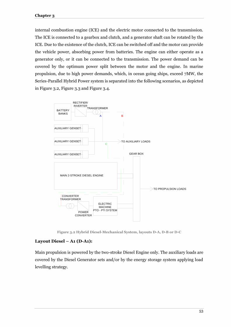
Chapter 3
53
internal combustion engine (ICE) and the electric motor connected to the transmission.
The ICE is connected to a gearbox and clutch, and a generator shaft can be rotated by the
ICE. Due to the existence of the clutch, ICE can be switched off and the motor can provide
the vehicle power, absorbing power from batteries. The engine can either operate as a
generator only, or it can be connected to the transmission. The power demand can be
covered by the optimum power split between the motor and the engine. In marine
propulsion, due to high power demands, which, in ocean going ships, exceed 7MW, the
Series-Parallel Hybrid Power system is separated into the following scenarios, as depicted
in Figure 3.2, Figure 3.3 and Figure 3.4.
Figure 3.2 Hybrid Diesel-Mechanical System, layouts D-A, D-B or D-C
Layout Diesel – A1 (D-A1):
Main propulsion is powered by the two-stroke Diesel Engine only. The auxiliary loads are
covered by the Diesel Generator sets and/or by the energy storage system applying load
levelling strategy.
MAIN 2-STROKE DIESEL ENGINE
AUXILIARY GENSET
AUXILIARY GENSET
AUXILIARY GENSET
ELECTRIC
MACHINE
PTO - PTI SYSTEMPOWER
CONVERTER
CONVERTER
TRANSFORMER
BATTERY
BANKS
GEAR BOX
TO AUXILIARY LOADS
TO PROPULSION LOADS
A B
C
RECTIFIER/
INVERTERTRANSFORMER

Hybrid Power Systems
54
Layout Diesel – A2 (D-A2):
This layout refers to an All Electric Ship concept. No gearbox exists, the generators supply
energy to the electric motors to cover propulsion. The propulsive energy can be fully
covered by the generator sets or can be absorbed by the energy storage medium.
Generators can be either switched off when there is no need for excessive power, or can
charge the battery system. This layout is not suitable for slow speed vessels, as the direct
propulsion has been proven more energy efficient (Molland et al., 2012).
Figure 3.3: Hybrid- All Electric Ship Propulsion layout (D-A2 concept)
Figure 3.4: Line Diagram of the proposed D-A2 concept
AUXILIARY GENSET
AUXILIARY GENSET
AUXILIARY GENSET
PROPULSION
MOTOR
POWER
CONVERTER
CONVERTER
TRANSFORMER
BATTERY
BANKS
GEAR BOX
TO AUXILIARY LOADS
TO PROPULSION LOADS
RECTIFIER/
INVERTERTRANSFORMER
PROPULSION
MOTOR
POWER
CONVERTER
CONVERTER
TRANSFORMER
AUXILIARY GENSET
AUXILIARY GENSET
AUXILIARY GENSET
HYBRID
CONTROLLER
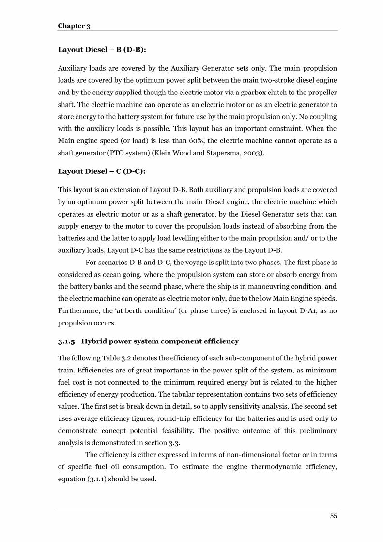
Chapter 3
55
Layout Diesel – B (D-B):
Auxiliary loads are covered by the Auxiliary Generator sets only. The main propulsion
loads are covered by the optimum power split between the main two-stroke diesel engine
and by the energy supplied though the electric motor via a gearbox clutch to the propeller
shaft. The electric machine can operate as an electric motor or as an electric generator to
store energy to the battery system for future use by the main propulsion only. No coupling
with the auxiliary loads is possible. This layout has an important constraint. When the
Main engine speed (or load) is less than 60%, the electric machine cannot operate as a
shaft generator (PTO system) (Klein Wood and Stapersma, 2003).
Layout Diesel – C (D-C):
This layout is an extension of Layout D-B. Both auxiliary and propulsion loads are covered
by an optimum power split between the main Diesel engine, the electric machine which
operates as electric motor or as a shaft generator, by the Diesel Generator sets that can
supply energy to the motor to cover the propulsion loads instead of absorbing from the
batteries and the latter to apply load levelling either to the main propulsion and/ or to the
auxiliary loads. Layout D-C has the same restrictions as the Layout D-B.
For scenarios D-B and D-C, the voyage is split into two phases. The first phase is
considered as ocean going, where the propulsion system can store or absorb energy from
the battery banks and the second phase, where the ship is in manoeuvring condition, and
the electric machine can operate as electric motor only, due to the low Main Engine speeds.
Furthermore, the ‘at berth condition’ (or phase three) is enclosed in layout D-A1, as no
propulsion occurs.
Hybrid power system component efficiency
The following Table 3.2 denotes the efficiency of each sub-component of the hybrid power
train. Efficiencies are of great importance in the power split of the system, as minimum
fuel cost is not connected to the minimum required energy but is related to the higher
efficiency of energy production. The tabular representation contains two sets of efficiency
values. The first set is break down in detail, so to apply sensitivity analysis. The second set
uses average efficiency figures, round-trip efficiency for the batteries and is used only to
demonstrate concept potential feasibility. The positive outcome of this preliminary
analysis is demonstrated in section 3.3.
The efficiency is either expressed in terms of non-dimensional factor or in terms
of specific fuel oil consumption. To estimate the engine thermodynamic efficiency,
equation (3.1.1) should be used.

Hybrid Power Systems
56
6 6 6
3,6 10 3,6 10 3,6 10eng
u f u e u eF
P P P
Q m P b b
(3.1.1)
where,
P : Engine output power [kW]
QF : Chemical output power of fuel [kW]
Θu : Low calorific value of fuel [kJ/kg]
be : Specific fuel consumption of Diesel engine [g/kwh]
The problem of propulsive efficiency is complex, as the engine speed has significant
influence over the efficiency of the propeller (constant pitch) and the thermodynamic
efficiency of the engine. Based on (3.1.1), it is clear that the decreased engine speed leads
to higher SFOC, resulting in lower fuel efficiency.
Table 3.2: Hybrid System component efficiencies (Chatzilau et al. 2006, Prousalidis et al. 2003, Greig and Bucknall, 2012)
Component Description Necessary in
layout Simulation use
Efficiency Conceptual use
Efficiency
Battery Converter and Transformer
All layouts 98%
Total conversion
efficiency 92%
Transmission losses All layouts 99.5%
Gearbox efficiency A1, B, C 98%
Motor Converter Transformer
B, C 99%
Electric Machine Power Converter
A2, B, C 96%
Electric Machine A2, B, C Figure 3.7
Electric generator All layouts Figure 3.8
Sodium Nickel Chloride Battery
All layouts Figure 3.5 Figure 3.6
Round trip 92%
Redox Flow Batteries All layouts - Round trip
85%
Two-stroke Slow Speed Diesel Engine
A1, B, C Figure 3.9 Minimum SFOC
175g/kWh
The second key component of the Hybrid system is the energy storage medium.
This system consisted solely of batteries. Therefore, in order to implement the behaviour
of the battery to the calculations, the terms open voltage, closed voltage and nominal
voltage have to be explained. Thus, the theoretical voltage is dependent only on the
materials of anode and cathode, the composition of the electrolyte and the temperature
Linden and Reddy (2002). This means that it is independent of the operational profile of

Chapter 3
57
the storage system. The open circuit voltage in the battery voltage under no-load is greater
than the nominal voltage, which is the typical operating voltage of the battery. During
discharge, the battery voltage is lower than the theoretical voltage.
This difference arises as electric current passes through the electrodes and polarisation
occurs, which accompanies the electrochemical reactions (Linden and Reddy: Broadhead
and Kuo, 2002). The losses include the activation polarisation, which is an inevitable
process in order to start the reaction at the electrode surface, and concentration
polarisation, which occurs due to the difference in concentration of the reactants. The
product of these effects is waste heat. However, the waste heat is also increased by the
internal impedance of the battery and is referred to as Ohmic polarisation. To summarise,
the useful energy that can be drained out of the battery is given by the following equation
(Linden and Reddy: Broadhead and Kuo, 2002):
0 ct c ct c ia a c cE E i R i R (3.1.2)
where,
E0 : electromotive force or open-circuit voltage of cell
(ηct)a, (ηct)c : activation polarisation or charge-transfer overvoltage a at anode/cathode
(ηc)a, (ηc)c : concentration polarisation at anode and cathode
i : operating current of battery on load
Ri : internal resistance of the battery
The Sodium Nickel Chloride discharge and charge behaviour was presented in Dustman
(2004). The equivalent Ohmic Resistance of equation (3.1.2) can be acquired. However,
for the purpose of this project, detailed laboratory measurements have been supplied. The
battery discharge efficiency had been measured in the laboratory environment of a 557V,
32Ah battery for a set of discharge currents. The voltage drop had been measured until the
state of Charge (SoC) reached zero (fully depleted battery pack) (Manzoni et al., 2008). By
applying equation (3.1.2), the Resistance is then approximated. The voltage drop describes
the energy losses of the battery, thus the discharge efficiency is calculated and Figure 3.5
is introduced. It can be extracted from Figure 3.5 that the discharge efficiency is very high
when the discharge current is less than 2 A. However, the efficiency drop is significant
because of the interpolation between the measured value at 2A discharge current and the
theoretical value at 0A discharge current which is 100%.

Hybrid Power Systems
58
Figure 3.5: Experimental Sodium Nickel-Chloride battery efficiency mesh versus Depth of Discharge and Discharge Current
Based on the observed high efficiency bellow 2A, the sizing of the battery system should be
made in a way that the operational discharge current per battery string is less than this
value. Moreover, the reference State of Charge, where the battery system will maintain its
charging, should be in areas where the discharge efficiency exceeds 94%. Manzoni et al.
(2008) state the cycling should occur around 50% of the battery SoC for cycling purposes.
For load leveling needs, the cycle should be around 100% and 20% of the SoC.
In order to estimate charging efficiency versus charge current, an energy
approach was used and measurements were obtained in the laboratory environment.
Moreover, the charging current was varied from 2A to 15A. Nonetheless, the charging
voltage was set at 2.67V/cell, while the open circuit voltage (VOC) is 2.58V. Therefore,
accounting only for the voltage difference, it can be estimated that the efficiency is around
97%. Theoretically, the charge efficiency reaches 100% when it occurs in ultra- low
currents. Consequently, in order to estimate the charge efficiency in less than 2A, an
interpolation spline between 100% and the measured 97% is proposed. By taking into
account energy losses in charging, Figure 3.6 is introduced.
Chapter 3
59
Figure 3.6: Experimental curve of Sodium Nickel-Chloride battery efficiency versus charge current
Based on the laboratory findings, the State of Charge has negligible effect on the efficiency
and, for simplicity purposes, it can be assumed that the connection between SoC and
charge efficiency is linear. Thus the latter can be implemented as a single curve versus the
discharge current.
The electric machine that is present in Conventional Diesel Hybrid layouts D-B and
D-C has an efficiency that is dependent on the operating load and on the rotational speed.
Assuming that the rotational speed, which is controlled by the converter, remains
practically at the most efficient area, the total motor/generator efficiency is considered
dependent only on the load. As a result, Figure 3.7 is introduced. This curve was acquired
from on board measurements by the author during a shipboard energy audit. However, it
has to be stated that it was expected that the efficiency curve shape between the 75% and
100% would be flatter, increasing the overall motor efficiency. Nevertheless, changes in
efficiencies are crucial for the feasibility of the system and it was for this purpose that a
sensitivity analysis was performed.
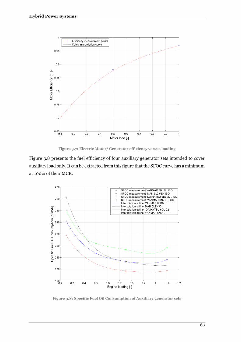
Hybrid Power Systems
60
Figure 3.7: Electric Motor/ Generator efficiency versus loading
Figure 3.8 presents the fuel efficiency of four auxiliary generator sets intended to cover
auxiliary load only. It can be extracted from this figure that the SFOC curve has a minimum
at 100% of their MCR.
Figure 3.8: Specific Fuel Oil Consumption of Auxiliary generator sets
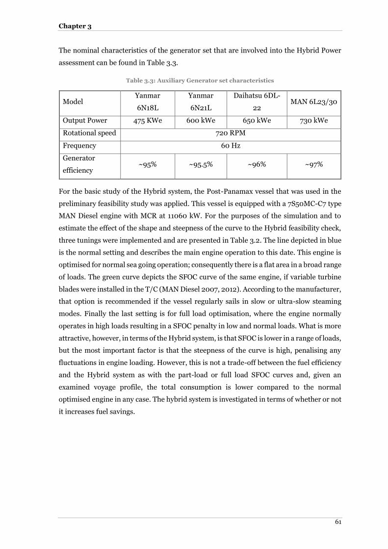
Chapter 3
61
The nominal characteristics of the generator set that are involved into the Hybrid Power
assessment can be found in Table 3.3.
Table 3.3: Auxiliary Generator set characteristics
Model Yanmar
6N18L
Yanmar
6N21L
Daihatsu 6DL-
22 MAN 6L23/30
Output Power 475 KWe 600 kWe 650 kWe 730 kWe
Rotational speed 720 RPM
Frequency 60 Hz
Generator
efficiency ~95% ~95.5% ~96% ~97%
For the basic study of the Hybrid system, the Post-Panamax vessel that was used in the
preliminary feasibility study was applied. This vessel is equipped with a 7S50MC-C7 type
MAN Diesel engine with MCR at 11060 kW. For the purposes of the simulation and to
estimate the effect of the shape and steepness of the curve to the Hybrid feasibility check,
three tunings were implemented and are presented in Table 3.2. The line depicted in blue
is the normal setting and describes the main engine operation to this date. This engine is
optimised for normal sea going operation; consequently there is a flat area in a broad range
of loads. The green curve depicts the SFOC curve of the same engine, if variable turbine
blades were installed in the T/C (MAN Diesel 2007, 2012). According to the manufacturer,
that option is recommended if the vessel regularly sails in slow or ultra-slow steaming
modes. Finally the last setting is for full load optimisation, where the engine normally
operates in high loads resulting in a SFOC penalty in low and normal loads. What is more
attractive, however, in terms of the Hybrid system, is that SFOC is lower in a range of loads,
but the most important factor is that the steepness of the curve is high, penalising any
fluctuations in engine loading. However, this is not a trade-off between the fuel efficiency
and the Hybrid system as with the part-load or full load SFOC curves and, given an
examined voyage profile, the total consumption is lower compared to the normal
optimised engine in any case. The hybrid system is investigated in terms of whether or not
it increases fuel savings.
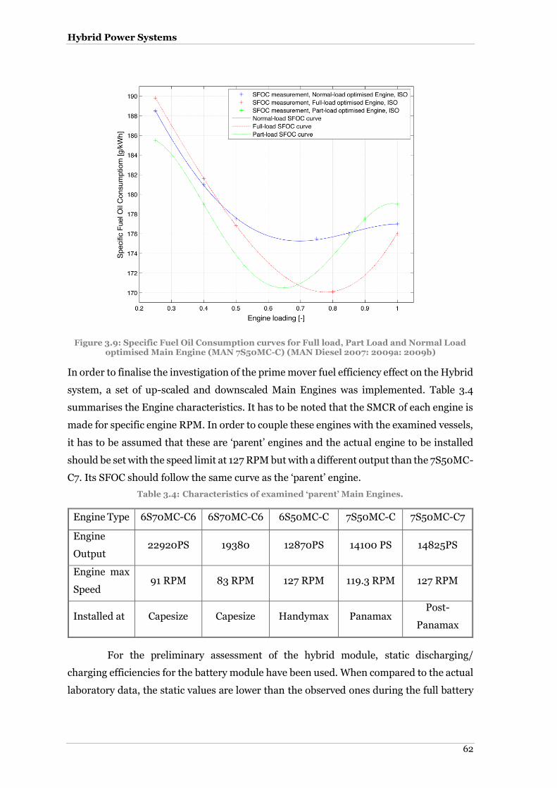
Hybrid Power Systems
62
Figure 3.9: Specific Fuel Oil Consumption curves for Full load, Part Load and Normal Load optimised Main Engine (MAN 7S50MC-C) (MAN Diesel 2007: 2009a: 2009b)
In order to finalise the investigation of the prime mover fuel efficiency effect on the Hybrid
system, a set of up-scaled and downscaled Main Engines was implemented. Table 3.4
summarises the Engine characteristics. It has to be noted that the SMCR of each engine is
made for specific engine RPM. In order to couple these engines with the examined vessels,
it has to be assumed that these are ‘parent’ engines and the actual engine to be installed
should be set with the speed limit at 127 RPM but with a different output than the 7S50MC-
C7. Its SFOC should follow the same curve as the ‘parent’ engine.
Table 3.4: Characteristics of examined ‘parent’ Main Engines.
Engine Type 6S70MC-C6 6S70MC-C6 6S50MC-C 7S50MC-C 7S50MC-C7
Engine
Output 22920PS 19380 12870PS 14100 PS 14825PS
Engine max
Speed 91 RPM 83 RPM 127 RPM 119.3 RPM 127 RPM
Installed at Capesize Capesize Handymax Panamax Post-
Panamax
For the preliminary assessment of the hybrid module, static discharging/
charging efficiencies for the battery module have been used. When compared to the actual
laboratory data, the static values are lower than the observed ones during the full battery
Chapter 3
63
simulation. Thus, the most of the performance aspects are not captured but it valid to
assume that fir at least these static efficiency values, the system is feasible and operational.
It is assumed that the operation of an equivalent Diesel-Electric system has the
minimum SFOC of each vessel’s current propulsion engine. Although the engine shop test
curve shows that the SFOC curve is almost flat near the optimum area, the actual measured
consumption differs significantly due to HFO operation and due to actual engine ship
interaction. In addition, based on shipboard energy audit measurements, the SFOC curve
shape may differ from the one supplied at the engine shop tests. However, when air and
sea and air temperatures are not globally available, no correction is assumed that
introduces error to the calculations. The overall battery performance cycle efficiency
(charging/discharging) is considered constant for a broad range of discharge currents that
the system is likely to operate, and equal to 85% for redox flow batteries (Mohamed et al.,
2009) and 92% for Sodium Nickel Chloride (Dustmann, 2004). These values for high
instantaneous discharge currents will drop, but over an overall cycle (which is denoted as
a battery operation with both discharging and charging modes during the examined time
frame) it should adequately represent the battery behaviour. Moreover, a 4% extra energy
loss is applied to the total battery operation, because the electric current has to be
transformed to mechanical energy at the electric motor and vice versa. In addition to the
hybrid part, the conversion losses from electrical to mechanical energy are typically 8% -
12%. The achieved efficiency values range from 95-97% for generators, 96% for frequency
converters and 95-97% for electric motors with the potential to be increased in the future.
Thus, the overall system efficiency from the diesel engine’s shaft to the propeller varies
from 85-92% dependent on the system load. For the D-A2 conceptual case, the
electromechanical conversion losses are taken equal to 8%.

Hybrid Power Systems
64
3.2 Conceptual case based on voyage statistical analysis
The following procedure is based on actual fleet data for various laden and ballast voyages
for Handysize, Handymax, Panamax, Post-Panamax and Capesize bulk carriers. A
complete Hybrid Power system is proposed based on the average discharging/ charging
efficiencies of the battery system.
Statistical power analysis
Daily ship performance data was collected from the technical department of a Greek
Maritime Corporation. Each technical form includes the daily maintenance and
monitoring logs, together with operational orders for ship routing. These forms are
commonly known as ‘noon reports’ and an example is shown in Table 3.5. Although these
forms contain important information about the ship’s performance, unfortunately, errors
made by the Chief Engineer or captain, due to the rush and repetition of measurements,
do exist and there are cases where values do not represent the actual voyage
characteristics. Thirty-one separate voyages across five vessel types and for a variety of
laden and ballast conditions were collected.
The engine loading, as a percentage of the maximum continuous rating of the
engine (MCR), was calculated by correlation of direct and indirect influence factors with
the shop tests of the propulsion engine. Direct influence parameters are the engine RPM,
the Fuel Admission Lever, the exhaust temperature (which should be corrected for engine
RPM as well) and the rotational speed of the turbochargers. Secondary parameters are the
slip of propeller, the ship’s speed, the wind direction and force, the sea conditions, and the
current strength and direction. These parameters have an indirect influence on the
correlation with the shop tests, but are the main reason why the engine loading varies. In
order to estimate the engine loading, the direct influence factors are interpolated into the
performance curves of the engine 2 . Based on the fuel admission lever, an initial
approximation of the loading is obtained. The fuel admission lever shows the actual
petroleum that is injected per cycle. The estimated load is then compared to the calm water
engine loading, which is described by the load indicator values. The latter shows the
desired engine loading, which displays the percentage of the MCR that the engine should
be operating at. If it is assumed that the engine Turbocharger is operating at the designed
operational envelope, meaning near the surge line, its rotational speed is unique in every
engine load. This actually defines the actual power loading of the engine, because the
rotational speed of the turbocharger is defined by the exhaust gas mass flow and from the
2 Data available at Fluid Structure Interaction research group at University of Southampton.
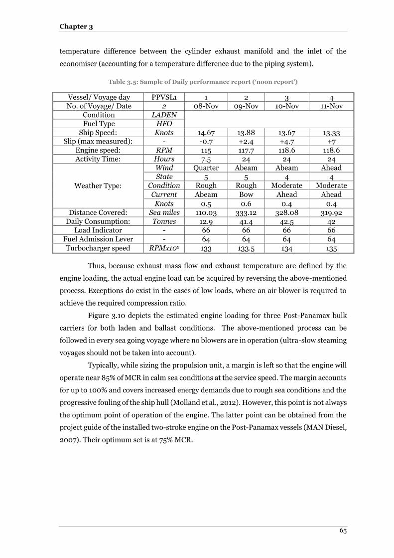
Chapter 3
65
temperature difference between the cylinder exhaust manifold and the inlet of the
economiser (accounting for a temperature difference due to the piping system).
Table 3.5: Sample of Daily performance report (‘noon report’)
Vessel/ Voyage day PPVSL1 1 2 3 4 No. of Voyage/ Date 2 08-Nov 09-Nov 10-Nov 11-Nov
Condition LADEN
Fuel Type HFO
Ship Speed: Knots 14.67 13.88 13.67 13.33 Slip (max measured): - -0.7 +2.4 +4.7 +7
Engine speed: RPM 115 117.7 118.6 118.6 Activity Time: Hours 7.5 24 24 24
Weather Type:
Wind Quarter Abeam Abeam Ahead State 5 5 4 4
Condition Rough Rough Moderate Moderate
Current Abeam Bow Ahead Ahead
Knots 0.5 0.6 0.4 0.4
Distance Covered: Sea miles 110.03 333.12 328.08 319.92
Daily Consumption: Tonnes 12.9 41.4 42.5 42 Load Indicator - 66 66 66 66
Fuel Admission Lever - 64 64 64 64
Turbocharger speed RPMx102 133 133.5 134 135
Thus, because exhaust mass flow and exhaust temperature are defined by the
engine loading, the actual engine load can be acquired by reversing the above-mentioned
process. Exceptions do exist in the cases of low loads, where an air blower is required to
achieve the required compression ratio.
Figure 3.10 depicts the estimated engine loading for three Post-Panamax bulk
carriers for both laden and ballast conditions. The above-mentioned process can be
followed in every sea going voyage where no blowers are in operation (ultra-slow steaming
voyages should not be taken into account).
Typically, while sizing the propulsion unit, a margin is left so that the engine will
operate near 85% of MCR in calm sea conditions at the service speed. The margin accounts
for up to 100% and covers increased energy demands due to rough sea conditions and the
progressive fouling of the ship hull (Molland et al., 2012). However, this point is not always
the optimum point of operation of the engine. The latter point can be obtained from the
project guide of the installed two-stroke engine on the Post-Panamax vessels (MAN Diesel,
2007). Their optimum set is at 75% MCR.

Hybrid Power Systems
66
Figure 3.10: Estimated engine loading for laden and ballast voyages of Post-Panamax ships
From Figure 3.11 it can be observed that in every voyage of the Post-Panamax vessels
within the fleet, the engine mean load varies from 70% to 80% of the MCR. It can also be
observed that the 9-day voyage in ballast condition (marked with blue boxes in Figure
3.10) has the largest fluctuations in the daily engine loading. Based on the reports from
that voyage, the ship faced extreme weather exceeding sea state 6, attempting, however, to
maintain a speed of 13 knots. However, the vessel voluntary reduced speed on the 6th, 8th
and 9th day. Based on the obtained reports, it can be extracted that small length voyages
have consistency in their reports, something that is not the case in long voyages such as
the 32-day voyage denoted with the black reversed triangle. For that reason, it was
attempted to regain the consistency mainly by altering the vessel speed, which normally is
calculated by the crew by dividing the distance by the voyage time without accounting for
the weather conditions, the propeller slip and the underwater current.
During the observation period of the fleet, the vessels were frequently cleaned
underwater during port stay to minimise the frictional resistance due to fouling. This
approach was implied directly by the management of the company. The aim was to
maximise the vessel speeds in order to increase the number of charters per year.
Taking into account the operational envelope, the equivalent Hybrid Power
system should have the main propulsion engine (in case of conventional Hybrid) optimised

Chapter 3
67
near the loads depicted in Figure 3.11. The appropriate sizing of the energy storage medium
in cases of load variations will lead to a zero net energy demand, as in this system the
engine is constantly operating into a single point. The selection of this point is crucial as it
reduces the capacity of installed energy, thus the initial cost of the system. Concerning the
efficiencies of the battery system, it has already been stated that these are taken as
constants and lower than the expected.
Figure 3.11: Mean engine loading for three Post –Panamax sister ships for laden and ballast voyage
Using the reported power requirements shown in Figure 3.10, the equation (3.2.1) is
introduced, as from now; the Hybrid system is examined from an energy approach.
2
1
Energyt
tP t (3.2.1)
Thus, the energy requirements (integration results) are presented in Figure 3.12 for three
Post-Panamax ships used to illustrate the methodology.
The Hybrid system sizing utilises multiple diesel generator sets with different
electrical output and energy storage devices, such as batteries. The operational point of the
Hybrid system is taken as equivalent to the two stroke conventional plant predicted by
average loading in similar routes or by a ‘smart’ controller. The latter will interpret data
such as the state of charge of batteries, number of generators currently in operation, fuel
efficiency of each engine, estimated time of arrival (ETA) at destination port and the sea
state forecast. The decision constraints are the operation with the minimum number of
generators and the likely demanded energy availability at the end or beginning of the
voyage. The mathematical modelling of this controller is performed in Chapter 4.
0.66
0.68
0.7
0.72
0.74
0.76
0.78
0.8
0.82
Mea
n l
oa
d o
f E
ng
ine
[%M
CR
]
Ballast Laden

Hybrid Power Systems
68
Figure 3.12: Requested energy per day for every vessel and voyage type
The operation of the Hybrid system is initially considered to function at discrete loads of
the equivalent conventional propulsion engine. For the D-A2 concept, the total power
output is formed by the algebraic sum of the optimum power output of each generator in
operation. As a result, the energy production is made having the lowest possible SFOC not
for a single load, but for every combination of maxima power outputs. These are referred
to as the ‘working points’ of the Hybrid system. Table 3.6 represents the closest working
point to the mean value of each voyage. Thus, the energy produced by the power output of
the working point is considered to cover the average propulsion energy demand for the
examined period. Nevertheless, it should be noted that, usually, generators intended for
propulsion follow a SFOC curve similar to the two-stroke engine. On the contrary,
generator sets oriented for auxiliary power have their optimised load near 100% of their
MCR. Thus, for this purpose it is imperative for the generators to be optimised for the
100% of the power output. The investigation involves the worst-case scenario of prime
mover selection, therefore the selected generator sets should be considered as propulsion
generators which follow a normal cubic SFOC curve with the minimum value around the
75% of the MCR. Nonetheless, this assumption increases the initial cost of the system as
the 25% of the power output is useless.

Chapter 3
69
Table 3.6: Working Point of equivalent propulsion system to cover the mean power requirements for the three Post-Panamax sister ships
Vessel: Laden Voyage Ballast Voyage 1 80% 80% 2 80% 80%
3 80% 70%
Importing the values from Table 3.6 and combining them with the results of
Figure 3.12, the energy distribution over the examined voyage duration is depicted in
Figure 3.13.
Figure 3.13: Example of energy fluctuation difference for laden and ballast Voyage of a Post-Panamax vessel (optimum point of operation is 75% of MCR) per day
This figure depicts the daily fluctuation of energy requirements for the vessel, if
the Hybrid Power system was in operation. The in operation generators produce a power
output equal to 80% of the conventional two-stroke engine MCR. However, the
requirements of propulsion vary with time, and the working point differs from the actual
energy demand. It should be noted that the working point comes from the statistical
analysis of similar voyages and denotes an operational point that minimises the need for a
large amount of installed energy. This minimisation occurs because the energy production
is made around that point instead of the optimum which can be located even 20% off the
actual operational point. Thus the standard deviation of the power demand is lower than
before, therefore the required energy capacity of the storage medium is reduced
accordingly. Judging from Figure 3.12, the energy storage medium, in order to meet the
propulsive requirement, is forced to supply energy when there is an excess of demand. In

Hybrid Power Systems
70
the opposite scenario, where the system has an excess of production, two potentials are
identified. In the first potential, the system has either to decide to reduce the number of
working generators, thus altering the working point and absorbing or storing energy. In
the second potential, when the fluctuation does not permit the first option, yields to store
energy to the energy storage medium without altering the engine loading. Option two is
applicable to conventional Hybrid system. Therefore, in the ideal operation of the system,
with no conversion losses and assuming a steady state time domain model, the green areas
above and below each working points should be equal. This implies that, after a voyage,
the system will have run in optimum condition and the storage medium will be fully
charged. When battery charge/discharge conversion losses exist, these areas have to be
equal with respect to the conversion losses. This means that the charging area (above the
operational point) is greater that the area below. This difference is equal to the loss of
power times the hours of operation.
Immediate conclusions for the energy storage installation and for the power
output can be extracted. It can be observed from Figure 3.13 that the amount of energy
that is available for storage, or is required to be supplied for the propulsion needs, is closely
related to the working point of the engine as it was previously defined. The selection of this
point can be further optimised and adjusted. Moreover, the installation of a Hybrid Power
unit potentially allows the main engine to be smaller, since in the event of rough weather
the extra amount of energy required for propulsion can be covered by the stored energy.
Sizing the Hybrid power system
The original ship design is assumed to remain constant so that the hull form and the
propeller are unaltered. Further fuel savings by subsequent modification of the hull form
were thoroughly discussed in Chapter 2. Hence, the overall system power delivered to the
propeller remains the same. Potential reductions in the installed power will be a result of
optimised selection of both engines and storage medium.
3.2.2.1 Sizing the Diesel prime movers
The installed engine on-board the examined Post-Panamax vessels is an MAN 7S50MC-
C7 engine with specified Maximum continuous Rating (SMCR) of 11060kW at 127 RPM.
The optimum point of operation is at 75% of the SMCR (MAN Diesel, 2007). In order to
size the Hybrid Power system, two potential layouts will be investigated. The first concept
includes six generator sets. With these six generators, 60% of the power will be supplied
by two identical engines and the remaining 40% by four identical diesel generators. This
selection is made in order to have larger engines which consume less fuel and for which
heat recovery is better. This enables the system to cover the working points as efficiently
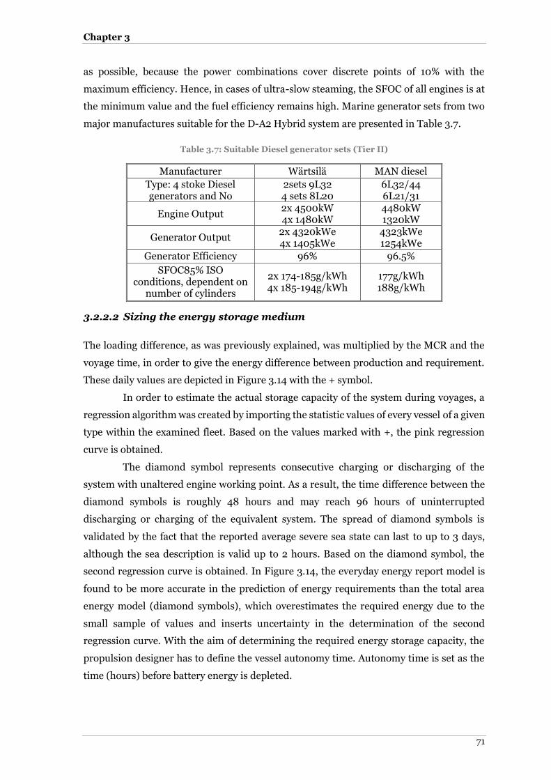
Chapter 3
71
as possible, because the power combinations cover discrete points of 10% with the
maximum efficiency. Hence, in cases of ultra-slow steaming, the SFOC of all engines is at
the minimum value and the fuel efficiency remains high. Marine generator sets from two
major manufactures suitable for the D-A2 Hybrid system are presented in Table 3.7.
Table 3.7: Suitable Diesel generator sets (Tier II)
Manufacturer Wärtsilä MAN diesel
Type: 4 stoke Diesel generators and No
2sets 9L32 4 sets 8L20
6L32/44 6L21/31
Engine Output 2x 4500kW 4x 1480kW
4480kW 1320kW
Generator Output 2x 4320kWe 4x 1405kWe
4323kWe 1254kWe
Generator Efficiency 96% 96.5%
SFOC85% ISO conditions, dependent on
number of cylinders
2x 174-185g/kWh 4x 185-194g/kWh
177g/kWh 188g/kWh
3.2.2.2 Sizing the energy storage medium
The loading difference, as was previously explained, was multiplied by the MCR and the
voyage time, in order to give the energy difference between production and requirement.
These daily values are depicted in Figure 3.14 with the + symbol.
In order to estimate the actual storage capacity of the system during voyages, a
regression algorithm was created by importing the statistic values of every vessel of a given
type within the examined fleet. Based on the values marked with +, the pink regression
curve is obtained.
The diamond symbol represents consecutive charging or discharging of the
system with unaltered engine working point. As a result, the time difference between the
diamond symbols is roughly 48 hours and may reach 96 hours of uninterrupted
discharging or charging of the equivalent system. The spread of diamond symbols is
validated by the fact that the reported average severe sea state can last to up to 3 days,
although the sea description is valid up to 2 hours. Based on the diamond symbol, the
second regression curve is obtained. In Figure 3.14, the everyday energy report model is
found to be more accurate in the prediction of energy requirements than the total area
energy model (diamond symbols), which overestimates the required energy due to the
small sample of values and inserts uncertainty in the determination of the second
regression curve. With the aim of determining the required energy storage capacity, the
propulsion designer has to define the vessel autonomy time. Autonomy time is set as the
time (hours) before battery energy is depleted.

Hybrid Power Systems
72
Figure 3.14: Energy charging/discharging during at sea operation, from voyage’s working point and application of regression analysis
It can be extracted that the data presented with the diamond symbols is related
to the ‘autonomy radius’ of the system. For the Marine Hybrid system, 96 hours autonomy
time of the system is considered sufficient for bulk carrier applications. The results for ‘at
sea operation’ for the bulk carrier fleet are summarised in Table 3.8, while the sizing
graphs can be found in Appendix III.
Table 3.8: Storage medium required energy capacity and maximum power output per vessel type for ‘at sea’ operation
Type of Vessel: Installed MWh: Power Output [kW]
Handysize 8 1
HandyMax 8 1
Panamax 15 2
Post-Panamax 5 2
Capesize 4 1
Although the size of the energy storage medium is presented in Table 3.8, more
aspects of energy availability have to be considered. It was previously mentioned that the
energy storage medium at the end of the voyage has to be fully charged. This requirement
is justified so the storage system has enough energy for sailing inside the Emission Control
Chapter 3
73
Areas (ECAs). In these zones, an ‘emission free’ battery only operation is ideal, something
which increases significantly the amount of stored energy and is dependent on the sailing
speed and distance until the pilot station. Moreover, in certain sizing scenarios, sufficient
stored energy has to be available for departure without engine operation while the cargo
handling had also been performed without ship engine operation. The latter potential is
possible when harbours are equipped with ‘cold ironing’ facilities. More energy demand
scenarios can be identified, however, only some of them can be implemented without
applied case specific storage capacity optimisation. Notwithstanding these variations, this
project the sizing is concentrated on the voyage phase and it is assumed that the battery
system is fully charged at the beginning and end of each voyage and these implications can
be solved by optimally increasing the storage medium in future work.
3.3 Feasibility analysis
The feasibility check of the Hybrid system is made for an AES Hybrid (scenario D-A2) and
a conventional Hybrid (D-B) system. A schematic representation of the investigated
layouts is made in Figure 3.2 and Figure 3.3. Layout D-A2 has as basis the AES concept.
The second scenario can be identified as a two-stroke Hybrid system with gearbox and
electric motor similar to Power Take Off/In (PTO-PTI). The latter systems are constantly
gaining ground in marine propulsion due to advantages in terms of safety and fuel
consumption (Griffiths, 2006). The efficiency of each subcomponent was presented in
section 3.1.5.
Operational feasibility based on voyage analysis
The voyage fuel consumption reported by the actual vessel is compared to the simulated
consumption of the Hybrid Diesel Electric system. The introduced uncertainty regarding
the on board fuel measurements and how the effect in this thesis is reduced was discussed
in Chapter 2.
The system is using the batteries to apply load levelling in propulsion demands,
hence discharge and charge are determined by the same operating loading profile of the
examined voyage. This system was simulated with the constraint of fully charged batteries
at the end of ‘at sea’ operation. Thus extra electricity, hence more fuel, is produced in order
to charge the system, if the net value of energy production is positive at the end of the time
period. The savings in terms of fuel using the Hybrid system are summarised in Table 3.9.
The likely annual fuel savings in terms of total emission contribution to global savings from
the bulk carrier shipping sector are presented in Table 3.10 for the maximum emission
savings related to fuel consumption only and operation of medium speed engines in
scenario D-A2. These values are the result of the projection of the acquired sample over

Hybrid Power Systems
74
the global number of vessels of the same type, and exclude the likely numbers of days in
port. It is clear that the number of vessels plays a significant role in the produced amount
of exhaust gasses (Eyring et al. 2005).
Table 3.9: Potential fuel savings, for D-A2 and D-B layouts per vessel type and for static efficiencies
Type of Vessel:
Number of
Vessels in world
fleet
Voyage Type:
Daily fuel savings
[tonnes/Day]
Voyage fuel savings [%]3
Single ship fuel
savings/year (Fuel: 520$/t)
up to [m.
USD/year]:
D-A2 D-B D-A2 D-B D-A2 D-B
Handysize 1,774 Laden 0.065 1.6 0.3% 7.7 %
0.27 0.50 Ballast 3.7 4.7 22.6% 28%
HandyMax 1,732 Laden 0 0.2 0% 0.7%
0.00 0.03 Ballast 0 0.13 0% 0.5%
Panamax 1,383 Laden 2.6 4.6 8.6% 15%
0.50 0.80 Ballast 2.8 4.8 9.6% 16%
Post-Panamax
98 Laden 5.3 8 12.3% 19%
0.80 1.30 Ballast 3.4 5.9 8.8% 15%
Capesize 722 Laden 0 3.6 0% 7.2%
0.00 0.60 Ballast 0 3.3 0% 7.5%
In order to calculate the emissions from the projected decrease in fuel
consumption through the application of Hybrid technology, the latter values were
multiplied by the corresponding fuel based factor, to give a global projected result of
emission savings per vessel category. As a subsequent step, the emissions savings were
multiplied by the percentage of vessels making up that category in order to give the
emission reduction results for the complete bulk carrier sector.
Finally, these values are multiplied by the percentage that this sector represents
of the world fleet, giving the extrapolated result of a 14% decrease in emissions that could
be achieved in the bulk carrier sector, using the maximum values of savings from the
voyage data analysed. This corresponds to a 1.8% reduction in the emissions of world
shipping. These projected savings are dependent on the voyage type, encountered weather
and desired speed of the vessel and thus represent an upper limit on the likely emissions
reductions that may be achieved through the adoption of Hybrid technology in this sector.
Nonetheless, a larger sample of voyage data should be investigated in order to verify the
projected values.
3 Voyage dependent savings

Chapter 3
75
Likewise, due to the fact that bulkers operate at low speeds and usually the
fluctuation of loading is considered small, faster ships and especially containerships that
share the largest CO2 emission percentage (depicted in Figure 1.1) benefit the most from
the Hybrid Power systems. Hence, if the proposed system is installed on these ships, the
reduction percentage for the global shipping could increase more significantly.
Table 3.10: Extrapolated for the global bulker fleet potential emission savings [m. tonnes/year] assuming 60% laden and 40% ballast voyages
Emission Gas: CO2 [m. tonnes/year] NOx [m.
tonnes/year] SOx [m. tonnes/year]
Voyage Type: Laden Ballast Laden Ballast Laden Ballast D-B
HandySize 1.800 3.500 0.050 0.098 0.030 0.060 HandyMax 0.230 0.095 0.006 0.003 0.004 0.002
Panamax 4.100 2.900 0.110 0.080 0.070 0.050 Post-Panamax 0.510 0.250 0.010 0.007 0.009 0.004
CapeSize 1.600 1.000 0.046 0.028 0.030 0.018
D-A2
HandySize 0.070 2.800 0.210 0.220 0.001 0.050
HandyMax 0.000 0.000 0.250 0.130 0.000 0.000
Panamax 2.300 1.700 0.320 0.210 0.042 0.030
Post-Panamax 0.330 0.140 0.028 0.014 0.006 0.003
CapeSize 0.000 0.000 0.180 0.120 0.000 0.000

Hybrid Power Systems
76
Financial feasibility based on voyage analysis
The type of storage system determines the economic feasibility of the Hybrid ship concept.
As seen in Dedes, et al. (2010) and described in section 3.1.2, the Vanadium Bromine redox
flow cell and the Sodium Nickel Chloride batteries are suitable candidates for Hybrid
power systems. Redox flow cells are reported to have a life period of more than 10000
cycles (Divya and Østergaard, 2009), while Sodium Nickel Chloride batteries have
reported life cycles of over 4000 (Dustman, 2004). Based on the reported estimated engine
loading and operating engines as described in Figure 3.10, ship operations are unlikely to
exceed 2500 cycles (full charging/discharging) over a 25 year period. As a result, no cost
for replacing the storage medium will be assumed. However, sets of complete voyage
simulations will define a mean number of cycles per voyage, which can be extrapolated to
identify vessel life time cycles.
The cost of the equivalent propulsion unit is increased compared to the
conventional two-stroke diesel. Aside from the storage medium cost, a difference in price
exists between large two-stroke diesel engines and smaller Diesel generators. The cost of
a propulsion system using this system is estimated by the Benford equation (3.3.1)
0.7
OTM MC A SHP (3.3.1)
where, AM is a constant and taken as equal to 2050$/kW (Mulligan, 2008).
The man hours of labour are given by equation (3.3.2)
0.30
MMHS 200001000
SHP
(3.3.2)
Where,
SHP : Shaft horse power [kw]
The total cost of the working labour is given by
MW KHRM MC =K ×MHS (3.3.3)
where, KMHRΜ = 30$ which is the man hour cost, (average ship yard labour cost, China is
excluded from the calculation (Mulligan, 2008)).
Such calculations indicate that the cost of the main engine is approximately
250$/kW. However, the typical cost of diesel generator engines is significantly higher than
the main engine. A typical price per kW of diesel generators is 350$/kW (Fragkopoulos,
2007). Although the initial cost of such engines is higher, the advantage of prefabrication

Chapter 3
77
and the modular application of the machinery components leads to savings in construction
man-hours by shortening the overall construction time of the vessel. Thus, the total
construction costs are potentially reduced (Prousalidis et al., 2003), although this
statement is not investigated further here. Furthermore, cost difference exists due to the
installation of electric motors, cabling and other components of the electrical installation.
An overall 6% increase in machinery cost will be assumed as the cost of the electrical
components. The machinery cost is taken to be 30% of the total cost of the ship
(Papanikolaou, 1991). Thus the extra machinery cost represents a 2% increase in the
overall price of the vessel. The market value of the vessels is taken according to the current
market state (Cotzias Shipping Group, 2010). Concerning the fuel price market, an average
value for the year is taken equal to 520$/tonne (Petromedia LTD, 2010). However, the
trend of fuel prices shows that its price is likely to increase in future years. As a result, a
rate of price increase of 10% each year is assumed. It is further assumed that after 25 years
the storage system can be sold for 10% of the original cost.
For an initial evaluation of the economics of the Hybrid concept, the dynamic
index of Internal Return Rate (IRR) is adopted. The income of the investment is that
calculated as fuel savings per year multiplied by the dynamically changing fuel prices.
0 1 11
n nj j
HYBRIDj jj J
FS CCost
( IRR )IRR
(3.3.4)
where, FSj is considered as ‘income’ of the investment and is equal to the calculated and
projected fuel savings per year per vessel and Cj are the maintenance costs as follows:
1
1
hybrid
j j
C OM
C C e
(3.3.5)
Table 3.9 shows the simulated fuel savings obtained by the optimisation of energy flow and
using the Hybrid technology on-board ships. Hence,
1 1 2j jFS FS e e (3.3.6)
where, OM Hybrid is equal to 0.08$/kWh for the Sodium Nickel Chloride batteries. For the
redox flow cell batteries, it is equal to 0.0008$/kWh.
The investment will be funded by a fixed interest rate bank loan. The rate (RL) is
equal to 8% and the loan payback period (NL) is 10 years. Every instalment amount is given
by the equation (3.3.7):

Hybrid Power Systems
78
1 (1 ) L
LLt FF
L
rA L
Nr
(3.3.7)
A Post-Panamax vessel ideally operates for 340 days per year on average and spends 60%
of the time in laden and 40% of the time in ballast condition (Psaraftis and Kontovas,
2008). A five-day period per month on average for charging/discharging is assumed as
port time. As a result maximum 280 days remain for voyages.
The Internal Rate of Return value provides a means to assess whether the initial
investment is worthwhile. A suitable threshold value of IRR is considered to be 10%
(Osborne, 2010). Every scenario above this value is considered worthwhile from a purely
economic perspective. In alternative cases, either the scenario is judged economically
unfeasible or potential improvements in technology, relative to the current state, will
improve the economic criterion of the investment. It should be noted that IRR values
depend on the fluctuating market costs of materials.
It is likely, as the market for large-scale energy storage systems increases, that
there will be corresponding reductions in costs. Table 3.11 presents calculated values of
IRR for each vessel type within the fleet examined and for the two storage media
considered. The results suggest that a system based on Sodium Nickel-Chloride batteries
is economically feasible in most vessel types and the payback period is very attractive.
Vanadium redox flow batteries, on the other have, seem to have potential in the future.
Table 3.11: Internal Rate of Return for conceptual Hybrid power layout
Type of Vessel: Installed
MWh: Storage System:
Internal Rate of Return:
Scenario 1: Scenario 2:
Handysize 8
Sodium Nickel-Chloride
11.5% >100%4
Vanadium Bromine 2.0% 25.1%
Handymax 8
Sodium Nickel-Chloride
0% 0%
Vanadium Bromine 0% 0%
Panamax 15
Sodium Nickel-Chloride
20.0% >100%4
Vanadium Bromine 1.4% 16.6%
Post-Panamax 5
Sodium Nickel-Chloride
71.7% >100%4
Vanadium Bromine 33.0% >100%4
Capesize 4
Sodium Nickel-Chloride
0% 61.6%
Vanadium Bromine 0% 27.6%
4 The value is >100% because in Handysize, Panamax, Post-Panamax, the payback period is 8, 19, 3 and 1 years respectively instead of 25 in other cases.

Chapter 3
79
Technical feasibility assessment
This section investigates the technical feasibility of energy storage devices installed on bulk
carriers through use of a systematic concept design variation. Likely values of energy losses
due to conversion are also considered. Through observation of engine variations and the
operational curves of the engine, the potential fuel savings of the Hybrid system are
compared to the conventional propulsion system. The Hybrid system assumes a scenario
of constant speed operation. Any variance in loading and any peak requirements will be
supplied from the storage system by applying load levelling to the system. Thus, diesel
engines are either switched off to reduce the total fuel consumption or are operated at
constant load resulting in the engine to be always loaded at the optimised consumption
point so to have the minimum Specific Fuel Oil Consumption (SFOC). In order to achieve
significant fuel savings, the variance should exceed a certain percentage determined from
the SFOC curve of the engine. The amount of fuel saving is dependent on the observed
fluctuations.
A system engineering approach is applied (Elliot and Dearsley, 2007), which is
holistic in its attempt to improve the Energy Efficiency Design Index (EEDI) of ships both
in terms of design and operation, although Hybrid ships are currently excluded from the
calculation of IMO. This requires an understanding of the trade-off between system
complexity and resultant new build cost against reductions in operational through-life cost
and exhaust emissions. The adopted methodology is presented and, through this, the
constructional and technical feasibility of the concept are demonstrated. The latter is
examined for new-builds based on a proposed and non-developed concept design together
with an investigation for retrofitting current designs for new-buildings, or on newly built
ships with a short operational life, with the Hybrid technology. In assessing the technical
feasibility, the calculation of engine room volume is critical and is performed first, along
with a record of all free spaces on board existing vessels. In addition, the weight calculation
and distribution are noted so that that any trim issues that might arise can be inserted in
the calculation of major loading conditions of the examined ship type. Finally, the energy
storage devices and the electric components are introduced and their weights and volumes
are inserted in calculations affecting the trim and filling of the free spaces. The new
components and the battery system have known volume and have to fit into the current
compartments as well as maintaining the Ship’s lightweight and with a minimal impact on
cargo capacity and hence economic viability of the initial vessel.
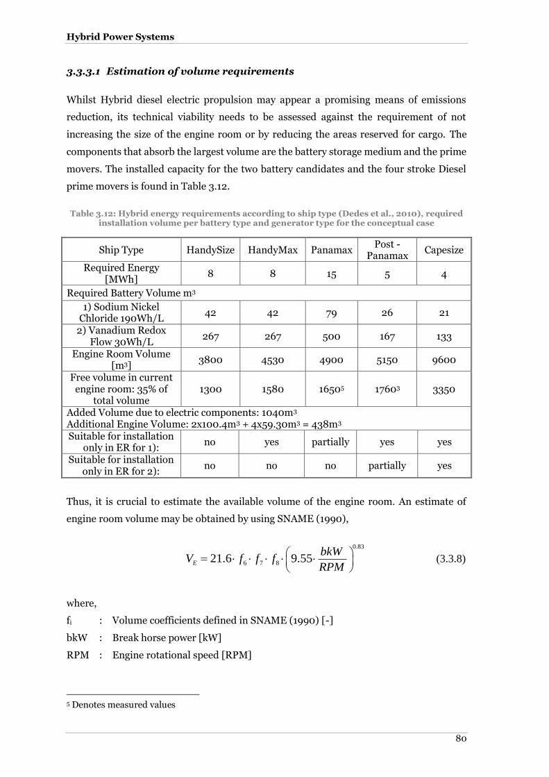
Hybrid Power Systems
80
3.3.3.1 Estimation of volume requirements
Whilst Hybrid diesel electric propulsion may appear a promising means of emissions
reduction, its technical viability needs to be assessed against the requirement of not
increasing the size of the engine room or by reducing the areas reserved for cargo. The
components that absorb the largest volume are the battery storage medium and the prime
movers. The installed capacity for the two battery candidates and the four stroke Diesel
prime movers is found in Table 3.12.
Table 3.12: Hybrid energy requirements according to ship type (Dedes et al., 2010), required installation volume per battery type and generator type for the conceptual case
Ship Type HandySize HandyMax Panamax Post -
Panamax Capesize
Required Energy [MWh]
8 8 15 5 4
Required Battery Volume m3
1) Sodium Nickel Chloride 190Wh/L
42 42 79 26 21
2) Vanadium Redox Flow 30Wh/L
267 267 500 167 133
Engine Room Volume [m3]
3800 4530 4900 5150 9600
Free volume in current engine room: 35% of
total volume 1300 1580 16505 17603 3350
Added Volume due to electric components: 1040m3 Additional Engine Volume: 2x100.4m3 + 4x59.30m3 = 438m3 Suitable for installation
only in ER for 1): no yes partially yes yes
Suitable for installation only in ER for 2):
no no no partially yes
Thus, it is crucial to estimate the available volume of the engine room. An estimate of
engine room volume may be obtained by using SNAME (1990),
0.83
6 7 821.6 9.55E
bkWV f f f
RPM
(3.3.8)
where,
fi : Volume coefficients defined in SNAME (1990) [-]
bkW : Break horse power [kW]
RPM : Engine rotational speed [RPM]
5 Denotes measured values

Chapter 3
81
On account of the fact that equation (3.3.8) does not describe modern designs, a direct
measurement was performed using vessel drawings. By this means, the actual volume of
the engine room for a Panamax type bulk carrier is 88% of that estimated by equation
(3.3.8). For a Post-Panamax type, the corresponding figure is 90%. These figures reflect
the more compact engines installed in modern designs. The volume used in subsequent
calculations is thus taken as 5150 m3.
In Appendix Table 3 of Appendix II, the volume of each engine room component
in a conventional two-stoke installation in a bulk carrier (Panamax and Post-Panamax
types) is presented. Where available, the weights of the components are cited. It can be
seen from this table that many items are not connected to the type of propulsion system
used and are associated with the operation of the vessel. These items are thus accounted
for in equivalent propulsion systems. Concerning the existence of pumps and other
hydraulics, a separation was attempted with the intention of justifying those that can be
replaced in an electric propulsion system, or even neglected.
Appendix Table 1 presents components representative of those installed in a
modern cruise ship with integrated full electric propulsion, equipped with conventional
propulsion shafts instead of podded propulsion units. The power output for propulsion of
such a vessel is four times the power required by a bulk carrier. The examined cruise vessel
is equipped with two Synchronous motors of 21MW rated power. Each one weighs
approximately 150 tonnes. Using this information, an approximation can be made for a
bulk carrier installation.
Recent technological improvements indicate that the weight for the same nominal
output (20MW) could be reduced to only 89 tonnes and with more compact dimensions
(Lewis, 2007). In subsequent calculations, the weight of an electric motor rated at 10MW
is taken as 75 tonnes. Although the extra volume for electric components is presented in
Appendix Table 1, the dimensions of rectifiers, inverters, transformers and other parts of
the circuits are relative to the number of generator sets. A general overview of the
dimensions and weights is given for the equipment list of the fleet of cruise ships that were
examined. The weight of the generator sets is lower that the weight of a conventional two-
stroke diesel. However, for large power outputs and depending on the propulsion system
design, more than two generator sets have to be installed. Hence the total weight of the
engines including the appropriate electrical motor can vary from -10% to +10% of the
equivalent conventional engine weight.
For the examined Post-Panamax type ship, the increase in weight is 1.7% and is
connected to the number of generator sets. The added weight for the propulsion system
also has to account for the added mass of the storage medium. Using the preliminary sizing
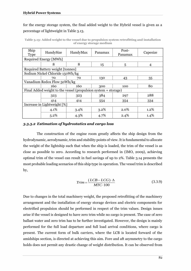
Hybrid Power Systems
82
for the energy storage system, the final added weight to the Hybrid vessel is given as a
percentage of lightweight in Table 3.13.
Table 3.13: Added weight to the vessel due to propulsion system retrofitting and installation of energy storage medium
Ship Type
HandySize HandyMax Panamax Post-
Panamax Capesize
Required Energy [MWh]
8 8 15 5 4
Required Battery weight [tonnes]
Sodium Nickel Chloride 150Wh/kg 70 70 130 43 35
Vanadium Redox Flow 50Wh/kg 160 160 300 100 80
Final Added weight to the vessel (propulsion system + storage)
323 323 384 297 288
414 414 554 354 334 Increase in Lightweight [%]
4.1% 3.4% 3.2% 2.0% 1.2%
5.2% 4.3% 4.7% 2.4% 1.4%
3.3.3.2 Estimation of hydrostatics and cargo loss
The construction of the engine room greatly affects the ship design from the
hydrodynamic, aerodynamic, trim and stability points of view. It is fundamental to allocate
the weight of the lightship such that when the ship is loaded, the trim of the vessel is as
close as possible to zero. According to research performed in (IMO, 2009), achieving
optimal trim of the vessel can result in fuel savings of up to 2%. Table 3.14 presents the
most probable loading scenarios of this ship type in operation. The vessel trim is described
by,
100
LCB LCGTrim
MTC
(3.3.9)
Due to changes in the total machinery weight, the proposed retrofitting of the machinery
arrangement and the installation of energy storage devices and electric components for
electrified propulsion should be performed in respect of the trim values. Design issues
arise if the vessel is designed to have zero trim while no cargo is present. The case of zero
ballast water and zero trim has to be further investigated. However, the design is mainly
performed for the full load departure and full load arrival conditions, where cargo is
present. The current form of bulk carriers, where the LCB is located forward of the
amidships section, is directed at achieving this aim. Fore and aft asymmetry to the cargo
holds does not permit any drastic change of weight distribution. It can be observed from

Chapter 3
83
the Table 3.14 that the full load departure condition has no trim. On the contrary, every
other condition has trim and, most of the time, ballast water. Any future weight
distribution of the current design requires a compromise between the full load departure
condition and the remainder of conditions in order to optimise trim and reduce the
amount of required ballast water.
Table 3.14: Loading Conditions of examined Post-Panamax bulk carrier
Condition Cargo
[tonnes]
Cargo Loss
%
Ballast [tonnes]
LCB [m]
LCG [m]
MTC [tm]
Trim [m]
Normal Ballast Departure
0 0.00 23414.3 117.126 117.189 1040.2 2.08
Normal Ballast Arrival 0 0.00 26061.1 114.757 114.855 1068.1 3.045
Heavy Ballast Departure
16487.1 0.00 23411.7 115.991 116.059 1226.5 2.667
Heavy Ballast Arrival 16487.1 0.00 24476.8 116.88 116.682 1191.4 2.265
Grain Departure SF65 60188.4 0.00 2250.7 116.664 116.702 1346.4 1.674
Grain Arrival SF65 60188.4 0.00 2250.7 118.866 118.879 1298.4 0.514
69990 tonnes DWT cargo Departure
65152.1 0.54 0 115.448 115.501 1364.5 2.323
69990 tonnes DWT cargo Arrival
65152.1 0.54 0 117.517 117.548 1331.3 1.205
Homogenous Design Departure
67858.4 0.52 0 115.656 115.702 1364.6 2.09
Homogenous Design Arrival
67858.4 0.52 0 117.668 117.693 1336.3 0.983
Grain Departure SF42 87866.1 0.40 0 116.837 116.841 1392 0.335
Grain Arrival SF42 87866.1 0.00 939.4 117.483 117.482 1384.9 0
Table 3.14 highlights the minimal cargo loss associated with the additional weight and
volume of the necessary equipment for the proposed Hybrid power installation, expressed
as a percentage of the cargo carried. The extra weight may be subtracted from the ballast
water, as added lightweight reduces this amount and when no ballast is present, this
weight reduces the cargo capacity. The worst case scenario is depicted in bold letters and
considered to be the minimum cargo capacity, with zero ballast, 100% filled fuel and fresh
water tanks, full provisions and minimum trim. The cargo loss is expressed as a percentage
of the initial loaded cargo.
It can be determined from Table 3.14 that cargo loss is related to the cargo
transported and to the presence of ballast water. The lower the cargo capacity of the vessel,
the higher the percentage cargo loss and vice versa (e.g. in Post-Panamax the cargo loss is
0.54% and reaches 0.78% for Panamax in Homogenous Loading).

Hybrid Power Systems
84
3.3.3.3 Design and construction parameters
In order to install the Hybrid power system components in existing ship designs, typical
general arrangements, profile and decks plans and structural drawings have to be studied.
The extra volume of the battery system and components of the fully electrified propulsion
system are given in Table 3.12. A proportion of this volume can be installed in the engine
room (E/R) if there is sufficient space. The major contributors to the required volume are
the components for the electrified propulsion system. It is important that these be installed
inside the engine room. An approximation of the engine room volume following
installation of the components is also presented. If the final available volume is
insufficient, other free and void spaces have to be selected in order to install the energy
storage system. For the battery arrays, the battery volume can be a significant proportion
of the total required volume. For example, in the case of a 15 MWh installation (Panamax
vessel), the required battery volume is almost 25% of the total volume required. A void
space is an enclosed space, with access and/or ventilation below the main bulkhead deck,
astern and forward of the cargo length of bulk carriers excluding spaces for dedicated water
ballast, carriage of cargo, storage of substances (e.g. HFO, provisions), installation of
machinery and space used by crew. This compartment is suitable for energy storage
devices since, being located at the fore peak it improves the zero trim condition. The
volume in certain designs approaches 1200m3. The space is accessible through manholes
from the Bosun’s store and the height of the compartment is sufficient for easy handling
and removal of components and inspection. However, the bow section of the vessel suffers
from movement and slamming, hence the behaviour of batteries subject to such motions
requires further investigation. Nevertheless, Common Structural Rules (CSR) and flooding
scenarios set high standards for the longitudinal strength of the ship in specific damage
conditions. This implies restrictions in weight allocation in forward and aft void or ballast
compartments, as in certain scenarios the calculated bending moments exceed the
maximum allowed value for the structural integrity.
Another potential void space is the lower stool of bulkheads above the double
bottom. The preferable selections have to be made as close to the forward perpendicular
(between cargo holds 5, 6, 7) as possible, in order to create a constant lever around the
amidships point. This space is accessible while cargo is present through manholes or
weather tight hatches on the main deck. However, the manhole openings are located inside
the involved or adjacent cargo hold, something that does not allow any repairs that involve
equipment removal. For the case of Sodium Nickel Chloride batteries, due to the increased
temperature, natural or mechanical ventilation of the energy storage areas should be
available. At the lower or upper stools, mechanical ventilation can be achieved using high

Chapter 3
85
speed electric motors that drive a fan. The heat exchange is proportional to the air mass
flow. Hence, a large number of air changes per hour is required. In bulk carriers that are
certified to carry dangerous goods, mechanical ventilation which is able to change 8 times
the capacity of the hold is installed with success. Thus, it is believed that heat exchange can
be made using this way and the location of the fans to be in mushroom type ventilators
located on top of the mast houses. Cases such as water or oil cooled battery packs can be
achieved mainly in double bottom areas in Forepeak tank and in lower stools. In smaller
vessels, such as handysize and handymax bulkers, a pipe tunnel at the centreline exists.
This pipe duct accommodates the bilge and ballast lines. There is free space to install a 3rd
pipe that will be responsible for energy storage cooling.
However, for maintainability, repair and regular visual control of the system,
potential spaces have to be well thought out. Each compartment has to be easy to inspect
and maintain without any cargo removal. In case of failure, or flooding, a manual
shutdown of the electric system has to be implemented. Meanwhile, each array of batteries
should have the capability of isolation in case of damage. The access of the battery arrays
though the pipe duct enable the inspection capability during the voyage. Moreover, the
access through man holes and the existence of a wagon inside the duct permit excessive
repairs and transfer of spares easily from the E/R.
On the other hand, the already mentioned forepeak void space should be
examined. Unfortunately, a cooling installation can increase the cost of the system and,
above all, limit the space reserved for battery equipment. Moreover, depending on the for
peak design, ventilation ducts may be difficult to install. It should be mentioned though
that additional space is required for the secondary circuits and systems of the battery. In
addition, for protection purposes, it is advisable to have a switchboard panel installed in
every compartment that stores a significant amount of energy, for minimisation of the
short circuit risk and the possibility of overall storage system failure. In addition, the
length of power cables that will run through pipes located on top of the main deck increase
also the cost. Moreover, dependent on the voltage and current, proper screen type cables
should be installed, so to decrease potential interference with the electronic remote control
and sensors of the ship. However, this problem is already covered by classification society’s
rules.
In the case of Redox flow batteries storage can be achieved in a similar manner as
with Heavy Fuel Oil (HFO). Tanks allocated in the double bottoms can be used. However,
these areas are mainly reserved for HFO storage in built vessels. According to the new
MARPOL regulations concerning the storage of heavy fuel oil, the wing side tanks will be
used instead of double bottom tanks. The regulation (Annex I regulation 12A) applies to
all new-buildings delivered after the 1st of August 2010. Thus, the double bottom space will

Hybrid Power Systems
86
be reserved for ballast water. As a result, the designs of new ships with minimum water
ballast influence the storage of the reactants, because these designs with a V shape hull
under the design waterline minimise the void spaces and limit the potential storage areas.
Though a reduction in fuel oil consumption was statistically demonstrated with the Hybrid
system, hence, the requirement to carry more HFO in tanks can be altered and space
reserved for HFO can now be used for the electrolyte reactants allowing a flexible
determination of storage areas. The largest environmental impact of Redox flow batteries
is the polypropylene tanks, the flow frames and the steel stacks (Rydh, 1999). Thus,
additional tank retrofitting should be made, in order to accommodate the reactants. Given
the industrial progress in marine paints, the coating of these tanks does not pose problems.
In addition, the location of the wing tank reserved for HFO is between the cargo hold and
the ballast water top side tank, so in cases of collision, the HFO or the battery reactant has
a penetration protection of a couple of meters. Hence, the risk of damage is significantly
reduced. Nonetheless, energy is required to pump the reactants towards the proton
exchange membrane. The latter should be always positioned inside the E/R so to be easily
monitored and maintained. Thus, area close to the E/R should be ideal positions in terms
of secondary energy loss. For both battery media, an existence of a deep tank forward of
the E/R bulkhead could be the best solution. If the volume of the deep tank would be
reserved for the energy storage system, then the access to this compartment can be made
using watertight doors, simplifying the access problem significantly. Nonetheless, the
weight distribution should be carefully studied.
Given that the allocation of the weight can be performed in an optimum way, a
selection of proposed compartments for housing the systems has to be performed.
However, before discussing these potential arrangements in detail, the following design
constraints affecting the overall ship design have to be examined.
The location and type of propulsor have to be selected, as does the location of the
superstructure. The superstructure and its associated air drag contribute to the overall
resistance of the vessel. Meanwhile, an optimum location of the bridge deck can allow
better navigation if it is located near the bow. In the case of a propeller, a shaft system is
required. The weight and the length of the shaft system are associated with the volume and
compartment arrangement at the stern. It is not optimum to have large shafts and this is
one of the reasons why a conventional two-stroke diesel engine is located as close as
possible to the stern. In that case, the engine room compartment has to be located at the
stern to house the main engine and the exhaust piping, which usually requires the
superstructure to be located on top of the engine room and astern. Therefore, there is no
capability to alter the design and allocate the weights differently.

Chapter 3
87
The potential of electric propulsion allows a different approach in the design of
the stern and overall layout of the ship. Electrified propulsion uses electric cables as the
medium for power transfer instead of mechanical connections, and this allows alternative
locations of the prime movers to be considered, with subsequent optimisation of the hull
form at the stern. However, the location of one or multiple engine rooms must be
combined with the constraints of available space for cargo holds. As a result, the bow and
stern are the most suitable spaces for machinery allocation. For a conventional electric
propulsion system, electric motors and a shaft system are required. Due to the small
dimensions of electric, motors the housing compartment can have limited dimensions in
length.
The combination of diesel electric and energy storage devices permits the use of
the void space above the electric motors for the installation of a part of the storage system,
while housing the steering gear system in the adjacent room. Prime movers can be
vertically installed in a bow compartment, while a boiler room and/or turbine generators
can exploit the rest of the space. Concerning the electric equipment (summarised in
Appendix Table 1), it is recommended that it be located in different rooms, preferably in
separate watertight compartments. For example, electric motors and control inverters
should be in the same watertight compartment. The converters, located in a dedicated
room, have to be situated as close as possible to the motors to reduce the length of the
cables. On the other hand, generators can be placed wherever the ship design allows it.
Concerning the superstructure decks, they can have the same use as before, while the
construction and the design should take into account the aerodynamic drag and the wave
spraying in case of slamming events.
An alternative approach with electric propulsion is the use of podded drives that
combine steering and propulsion capabilities and do not require any space for electric
motors inside the hull. However, a dedicated compartment for steering the pods is
essential. Any free space can be covered by a set of batteries, if an energy storage device is
applicable. On top of this compartment, mooring equipment and bosun store can be
constructed. The rest of the machinery, along with the rest of the battery storage system,
can be installed in the bow section. The discussion on the modifications in existing ship
designs has been presented in Dedes et al. (2013a).

Hybrid Power Systems
88
3.4 Chapter summary
This chapter presented the statistical analysis of a set of laden and ballast bulk carrier
voyages. The adopted energy approach formed the basis of the Hybrid Diesel layouts and
of the appropriate sizing of the Hybrid machinery components. The sizing of the system is
dependent on the statistical sample. It was found that an every-day mean analysis is
suitable for sizing the energy storage medium and the prime movers. Moreover, the sizing
of the battery system is defined by the operational point of the prime movers. For this
reason a detailed table with the proposed energy capacity and the maximum battery power
output was presented. Nonetheless, the statistical analysis revealed the need of a detailed
ship voyage simulation for accurate estimation of power demand. This simulator is
implemented mathematically in Chapter 4 while its representation in computer
environment is made in Chapter 5.
The examined Hybrid scenarios proved to be financially viable with high IRR,
constructively feasible, in terms of added volume and added mass to the vessel
displacement and lightweight respectively. A set of void spaces was considered for the
installation of the battery equipment such as the forepeak void space, the double bottom
tanks and areas inside the engine room. It was proved that the payload reduction is
negligible compared to the overall fuel savings and the vessel trim is reduced in many of
the important loading conditions. In the worst case scenario, the payload capacity was
reduced by 0.54% and the vessel was sailing even-keel during departure condition.
This chapter also demonstrated the complete Hybrid – Diesel. The energy storage
medium which inserts the hybridization degree in the power train is consisted of batteries.
The proposed battery technologies which were demonstrated as feasible for the Hybrid
layouts are the Sodium Nickel Chloride battery type and the Redox flow batteries which is
a novel battery type for Hybrid electric vehicles. Both technologies offer significant
advantages which were described. However, due to the maturity of Sodium Nickel Chloride
batteries and the durability in the marine environment, is used for the further analysis.
A set of auxiliary and propulsion ‘parent’ engines was selected for sizing
purposes. In addition, the machinery component efficiencies were presented in a tabular
or graphical way, in order to form the mathematical models which are presented in
Chapter 4.
Parts of this analysis where published in Energy Policy Journal (Dedes et al.,
2012a) and in Transactions of RINA (Dedes et al., 2013a).
Chapter 4
89
4 Mathematical Modelling
This chapter presents the governing equations that describe the Hybrid Power module and
the ship simulator. The mathematical modelling is separated into two logical parts. The
first part describes the governing equations of the Simulink® environment blocks which
are presented in Chapter 5, while the second part defines the governing equations of the
optimisation algorithm. The latter is responsible for the operation or not of the Hybrid
module. The results of the simulation and optimisation are described in Chapter 6. The
applied models in this thesis are proposed by the literature for this type of studies (Molland
et al. 2012; Schneekluth and Betram, 1998). When applicable, the original publication is
cited. Furthermore, IMO in the second green-house emission studies (IMO, 2009) accepts
the applicability of these models for accurate approximation of ship calm water and added
resistance.
4.1 Ship – Environment interaction modelling
This part defines the governing equations of the ship with the fluids around its hull. This
interaction entails a level of complexity and it is imperative to model the calm water
resistance, the added resistance, the hydrodynamic induced loads, the wind resistance,
and the propeller model. Finally, in order to simulate the marine environment, the
simulator can either import mean reported data, or a generation of environmental
parameters is required. Models and assumptions for the parameter generation are
described.
Calm water resistance approximation
In order to simulate the calm water resistance of a ship, a set of resistance approximation
methods was investigated. The reviewed resistance prediction methods are expressed by
means of a tabular and/or a graphical and/or a mathematical model. The mathematical
model contains the regression analysis equations. Resistance prediction methods using
regression analysis can be directly used for simulations. The other two formats can be
indirectly implemented in a computer environment. Typically, tabular data can be suitably
transformed using statistical methods to derive one or more equations from the data,
which are then utilised in the simulation code. In addition, tabular data can be represented
by interpolation. Graphical data can be treated in the same way as the tabular; however,
the precision depends on the quality of the graph and the number of selected key points.
Data handling is achieved by using interpolation methods such as linear interpolation,
Taylor’s 2nd order interpolation (Aughey, 1968) and Thrilheimer cubic spline (Versluis,
1977). At the higher and lower speed ranges, the resistance curves characteristically tend

Mathematical Modelling
90
to flatten out. Therefore, when extrapolating beyond the bounds of the speed range of any
method, linear extrapolation is assumed to best approximate this trend (Moody, 1996).
The methods examined for simulation are a combination of graphical and tubular,
and one method is based on regression analysis. Each method has restrictions in
applicability. Table 4.1 summarises the applicability of each method and its publication
date in order to determine whether that method is still valid for modern ship forms.
The first method was developed by Hoof and Nicholson (1948), and is intended for fast
vessels with prismatic coefficient lower than 0.80 (CP<0.80).
In 1954, Lap developed a calm water resistance method applicable to single screw
merchant vessels. The method was based on model testing of modern – for that period –
hull forms. Keller, in 1973, updated the method for application in large vessels with a high
block coefficient (CB). This method can be used for most normal and full ships in full load
condition, but with less accuracy for ships in light load condition (Journee, 1976).
In 1940, SSPA published a resistance method not directly applicable to bulk
carriers. It was based on a series of vessels with U hull form. The results were intended for
0.525< CB < 0.725.
Another method intended for bulk carriers is the Japanese single screw vessel
series, developed by the Shipbuilding Research Association of Japan in 1964. It was based
on 35 model tests in a testing basin. This method has been developed for fast slender ships
with CB ≤ 0.84 and the length to beam ratio should be less than or equal to 6.17 (L/B ≤
6.17).
Todd (1963) published a graphical method for resistance approximation for single
screw merchant ships. Adequate data can be derived from the series ‘60’ to calculate the
residual Resistance RR. Restrictions in block coefficient apply, and the applicability of the
method is dependent on the position of the LCB together with the Beam to Draft ratio
(B/T).
Guldhammer and Harvald (1974) published a graphic method that correlated the
data of Taylor, series 60, SSPA and NPL methods. The parent hull form that was used to
export results had no bulbous bow, destroyer stern type and normal shaped form. Due to
its limited applicability because of the ‘parent’ form, the results are corrected in order to
describe modern vessels. The method is intended for 0.15 ≤ Fn ≤ 0.45, 4 ≤ L/V1/3 ≤ 8 and
0.5 ≤ CP ≤ 0.85.
BSRA is a standard method of analysing speed trial results, published in 1964.
The shaft power curve is the basis for corrections, where resistance is added using a
derivative of the power curve (ITTC, 2002). The BSRA series was formed by independent
model sets, which were formed using a geometrically altered ‘parent’ form. To extend its
applicability and in order to interpolate different forms, four series where considered as

Chapter 4
91
basic. In order to apply the method and correlate the examined vessel to one of the ‘parent’
forms, the block coefficient should range from 0.65 ≤ CB ≤ 0.875 (Schneekluth and
Bertram, 1998).
Hollenbach analysed model tank tests during the period of 1980 to 1995. A total
of 433 model tests took place in the Vienna Ship Model Basin with the aim of improving
the reliability of performance prediction of modern cargo ships at the design stage.
Hollenbach’s method gives an envelope of resistance. This envelope gives a minimum
resistance that can be achieved after optimisation, as well as the regular resistance. Ballast
and Laden conditions are separated. The method can be easily computerised. The output
of the method is the residual resistance.
The total resistance is given by:
T F RR R R (4.1.1)
The residual resistance is given by:
2
2 10R R
B TR C V
(4.1.2)
where,
B : Ship’s Breadth [m]
T : Ship’s Depth [m]
V : Ship’s surge speed [m/s]
ρ : Water density [kg/m3]
The determination of Coefficient CR can be found in Schneekluth and Bertram (1998).The
frictional resistance is approximated by the ITTC 1957 formula. Thus,
2
2
0.075
2log 2F totalR V S
Rn
(4.1.3)
where,
Rn : Reynolds number [-]
Stotal : Wetted surface area approximation [m2]
The wetted surface area is approximated by:
2totalS k L B T (4.1.4)
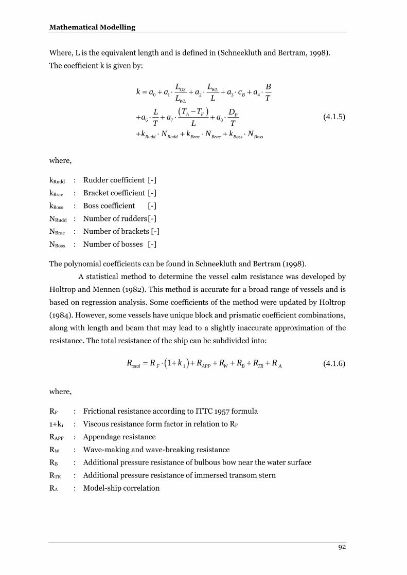
Mathematical Modelling
92
Where, L is the equivalent length and is defined in (Schneekluth and Bertram, 1998).
The coefficient k is given by:
0 1 2 3 4
6 7 8
OS WLB
WL
A F P
Rudd Rudd Brac Brac Boss Boss
L L Bk a a a a c a
L L T
T T DLa a a
T L T
k N k N k N
(4.1.5)
where,
kRudd : Rudder coefficient [-]
kBrac : Bracket coefficient [-]
kBoss : Boss coefficient [-]
NRudd : Number of rudders [-]
NBrac : Number of brackets [-]
NBoss : Number of bosses [-]
The polynomial coefficients can be found in Schneekluth and Bertram (1998).
A statistical method to determine the vessel calm resistance was developed by
Holtrop and Mennen (1982). This method is accurate for a broad range of vessels and is
based on regression analysis. Some coefficients of the method were updated by Holtrop
(1984). However, some vessels have unique block and prismatic coefficient combinations,
along with length and beam that may lead to a slightly inaccurate approximation of the
resistance. The total resistance of the ship can be subdivided into:
11total F APP W B TR AR R k R R R R R (4.1.6)
where,
RF : Frictional resistance according to ITTC 1957 formula
1+k1 : Viscous resistance form factor in relation to RF
RAPP : Appendage resistance
RW : Wave-making and wave-breaking resistance
RB : Additional pressure resistance of bulbous bow near the water surface
RTR : Additional pressure resistance of immersed transom stern
RA : Model-ship correlation

Chapter 4
93
The mathematical expression of the components that form the total Calm water resistance
using the Holtrop and Mennen (1982) method is given in Appendix I.
Table 4.1: Applicability range of calm water resistance approximation methods
Method Publication date Restrictions
Guldhammer-Harvald 1965, 1974 0.5< CP,WL < 0. 8 0.15 ≤ FnWL ≤ 0.44
4 ≤ LWL/1/3 ≤ 0.44
Taggart 1954 0.56< CP < 0.68 0.18 ≤ Fn ≤ 0.42
Danckwardt 1969
50≤ LPP ≤280 6 ≤ L/B ≤8 0.14 ≤ Fn ≤ 0.32 0.525 ≤ CB ≤ 0.825 2≤ B/T ≤3
Taylor-Gertler 1910, 1954, 1964
Fast Cargo Ships, warships Influence of bulb not taken into account Constant CM
Hoof – Nicholson 1948 Fast vessels with CP<0.80 Lap – Keller 1954 updated in 1973 Large slow ships with high CB
SSPA 1948-1959 1.5≤ B/T ≤6.5 0.525< CB < 0.75 0.18 ≤ Fn ≤ 0.32
Japanese single screw series
1964 CB ≤ 0.84 L/B ≤ 6.17
Todd (Series 60) 1963
0.6 ≤ CB ≤ 0.80 1.5%≤LCB≤2.5 from MidShip 2.5 ≤ B/T ≤3 or 0 ≤ B/T ≤3.5
Formdata method combining Todd and Guldhammer-Harvald
1974 0.15 ≤ Fn ≤ 0.45 4 ≤ L/V1/3 ≤ 8 0.5 ≤ CP ≤ 0.85
BSRA 1964 0.65 ≤ CB ≤ 0.875 Hotrop and Mennen 1982 - Hollenbach 1997, 1998 -
On the basis of method-implied restrictions, ease of programming into a
computerised environment and publication date, the Hollenbach and Holtrop-Mennen
methods are selected for simulation modelling.

Mathematical Modelling
94
Added resistance due to wind and waves
Ships operate in a changing environment driven by stochastic phenomena, and, in most
cases, they operate in rough conditions. The calm water resistance does not represent the
actual induced resistance due to wind and waves. Studies to estimate this effect were
performed and then continued mainly for tanker vessels. Maruo (1957; 1960; 1963)
attempted the first approach to added resistance estimation due to the motion of the ship
in waves. His method was used with the addition of the force created due to wave
reflection. Numerous studies on ship performance were performed and published by
Aertssen (1963; 1966), Aertssen et al. (1967), Aertssen and Van Sluys (1972), and detailed
speed performance monitoring using ship logs and satellite data was performed later by
Townsin et al. (1975). Aertssen (1969) introduced an approximate formula for the
calculation of ship speed loss in bad weather conditions. This formula was implemented
for the head weather case only. The formula is only dependent on Beaufort number, length
between perpendiculars, ship speed and constants dependent on Beaufort number.
Gerritsma and Beukelman (1972) used the general idea of Maruo’s approach,
introducing, however, the radiated energy approach for the calculation of the added
resistance of the ship in longitudinal waves. Salvensen et al. (1974) used the seakeeping
strip theory and radiated energy approach to produce more accurate results for the hull
designs. Townsin et al. (1975), after analysing a generalised system for speed performance
and monitoring, presented a simple formula for the speed loss of the vessels in head
weather. The formula was derived by monitoring the performance of large tankers. Fujii
and Takahashi (1975), Faltinsen et al. (1980), and Kwon focused on the issue of added
resistance due to wave reflection.
The Towsin and Kwon (1983) formula for speed loss due to added resistance was
updated by Kwon (2008) for a broader range of block coefficients (CB=0.55-0.85) and
Froude number (FN=0.05-0.30).
An alternative approach to the Kwon (2008) model was made by Grigoropoulos
et al. (2001), who published data of mean added resistance in a tabular form for a set of
seventy-two series 60 models in order to extrapolate the results to vessel specific designs.
The first attempt at tabular representation was made by Shintani and Inoue (1984). The
interpolation to the results is made using the L/B and B/T ratios, the CB the longitudinal
centre of buoyancy concerning the examined hull geometry. The sea condition during the
experiments was described by a two-parameter Bretchshneider spectrum (modal period
and significant wave height required). The results are given for wave angles and are non-
dimensional for the significant wave height.
Faltinsen et al. (1980), using a direct pressure integration approach, came up with
very interesting results, as well as setting a simple added resistance formula for the short

Chapter 4
95
waves added resistance due to the lack of efficiency of the generalised one. An improved
formula of Faltinsen et al. (1980) was published by Ohkusu (1984), which focuses on blunt
bow full hull forms while travelling at low speed. An overview of the methods for added
resistance in seaways was published by Wilson (1985). Naito (2008) calculated the added
resistance based on an improved version of Maruo’s approach, by using the Kochin
function. Kashiwagi (2009) took this further by inserting an enhanced unified theory.
The most recent studies have been performed by Liu et al. (2011), employing a 3D
frequency domain panel and a new Hybrid time domain Rankine source-Green function
method, and based on Mauro’s approach to calculate the added resistance of ship in waves.
Although models of added resistance contain the wind parameter in total
resistance, as in Aertssen (1967) and Towsin and Kwon (1983), dedicated studies have
been performed since the 60s. Shearer et al. (1960) have taken model testing
measurements and compared them to previous works of on-board measurements that
were published to that date. The effect of type and location of the superstructure was
highlighted. Moreover, they underlined that the absence of true wind experiments may
lead to an underestimated effect of wind resistance; hence the experimental setup differs
from the real voyage. Isherwood (1974) reviewed these published methods and proposed
a set of coefficients for roe and aft forces, lateral force and yawing moment. The data was
analysed by multiple regression techniques from model tests. This work was originally
submitted for written discussion; however, these coefficients describe with accuracy
modern designs up to the present day. The investigation of the wind effect was continued,
and van Berlekom et al. (1974) published equations that describe the forces of wind in large
tankers and large bulk carriers for laden and ballast voyages. Model tests were carried out
and the Norrbin mathematical model that described the simulations was used. In this
paper, the effect of rudder movements to keep the course straight was highlighted, as it
increases the total resistance. Furthermore, the rudder propeller interaction was inserted
in the calculations. The wind effect on the overall performance of the ship was later
updated by Willem and van Berlekom (1981). This approach was similar to the publication
of 1974, but contained model tests in modern hull and superstructure geometries, thus a
different set of equations was published. Blendermann (1994) published equations based
on twenty-eight model tests of present-day geometries. With respect to the aerodynamic
loading, there are only three basic ship types classified as rectangular cubes (car carriers,
ferries etc.), multiform shapes (containerships, cargo vessels etc.) and longitudinally
unsymmetrical shapes (supply vessels, tugs etc.). It is believed that these equations
accurately represent the wind effect on modern vessels.

Mathematical Modelling
96
4.1.2.1 The Aertssen model
Aertssen proposed a simple formula for approximation of the speed loss due to wind and
waves. By rearranging the proposed formula, the added resistance percentage is given by
equation (4.2.1)
2
1 1R V
R V
(4.2.1)
where,
ΔR : Added Resistance [N]
ΔV : Speed loss due to added resistance [m/s]The speed loss is determined by
equation (4.2.2)
pp
V mn
V L
(4.2.2)
where,
LPP : Ship’s length between perpendiculars [m]
m, n : Constants defined in Table 4.2 [-]
Table 4.2: Aertssen (1967) values for m and n coefficients
Head sea Beam sea Following sea BN m n m n m n 5 900 2 700 2 100 0 6 1300 6 1000 5 200 1 7 2100 11 1400 8 400 2 8 3600 18 2300 12 700 3
Aertssen considers the speed loss percentage constant in Beaufort numbers less than 5 and
equal to 10%.

Chapter 4
97
ABEAM
AHEAD
ASTERN
BOW
QUARTER
270
30
180
0
90
60
150
120
210
240
300
330
Figure 4.1: Wave and wind angles of attack in degrees and description terminology
4.1.2.2 The Towsin and Kwon model
In 1982, Towsin and Kwon updated the Aertssen formula. Constants have been chosen so
that the suggested formulae can closely represent the results of wind resistance by van
Berlekom (1981), wave reflection by the Kwon method, and ship motion resistance by
Maruo’s (1963) method. Thus the formulae intended to provide an estimate of the
percentage speed loss are given by equations (4.2.3) for tankers in laden, (4.2.4) and for
tankers in ballast and for containerships by equation (4.2.5), updated by Kwon (2008) for
larger range of Cb and Fn. The proposed formulae consist of two parts. The first part
denoted the effect of wind in added resistance and the second the effect of waves. In the
event that a mathematical model to represent the wind is present in the calculations, the
wind effect part must be omitted (Kwon, 2008).
6.5
2/3100% 0.5
2.7
V BNBN
V
(4.2.3)
6.5
2/3100% 0.7
2.7
V BNBN
V
(4.2.4)
6.5
2/3100% 0.7
22
V BNBN
V
(4.2.5)

Mathematical Modelling
98
where,
BN : Beaufort number which is defined by Henschke (1965) shown in Table 4.3
: Volume of displacement in [m3]
α : Correction factor for CB and Froude number given in Kwon (2008) [-]
μ is the correction coefficient of the wind and wave direction. The coefficient is given by
the set of equations described in (4.2.6).
2 0 0
2 0 0
2 0 0
2 1.7 0.03 4 30 60
2 0.9 0.06 6 60 150
2 0.4 0.03 4 150 180
bow
beam
following
BN
BN
BN
(4.2.6)
Table 4.3: Henschke (1965) sea description and correlation with Beaufort number and sea scale
Sea Scale Beaufort Number
(BN) Wind speed range
[m/s] Sea Description
0 0 0 - 0.2 Smooth sea 1 1 0.3 - 1.5 Calm rippling sea
2 2-3 1.6 – 5.4 Gentle sea
3 4 5.5 - 7.9 Light sea 4 5 8.0 - 10.7 Moderate sea 5 6 10.8 - 13.8 Rough sea 6 7 13.9 -17.1 Very rough sea 7 8-9 17.2 – 24.4 High sea 8 10 24.5 – 28.4 Very high sea
9 11-12 28.5 – 36.9 Extremely high sea
In cases where on-board observations are present (usually reported in ‘noon reports’), the
recorded sea description is converted to Beaufort number using the correlation of Table
4.3.
4.1.2.3 Detailed added resistance model
The application of the seakeeping methods discussed above produce response amplitude
operators (RAOs) (or transfer functions) for the examined vessels. As a result, when
running the seakeeping code, the RAO for the added resistance for a given angle of attack
can be acquired. Moreover, in order to produce a loading from the sea, the behaviour of
the latter can be described by a spectrum. The most commonly used sea spectra are the
JONSWAP, Bretschneider and the single parametric spectrum proposed by Pearson and
Moskovich. In order to obtain the response of the vessel to the given spectrum, the
following transformation should be made:

Chapter 4
99
2
AR ARS RAO S (4.2.7)
The sea spectrum Sηη(ω) is corrected for the encounter frequency. The relationship is valid
for deep water (depth> 90m) and is given by the following equation:
1
00
21 cos
VS S
g
(4.2.8)
where,
ω0 : Encounter frequency [rad/s]
For simulation purposes, it is essential to produce a time series of added resistance given
the ship’s speed, the sea spectrum and the wave angle of attack. The model by Pierson (St
Denis and Pierson, 1953) and Longuet-Higgins (1952) is commonly used in the literature.
It is based on the idea that random cosine wave is expressed by a large number of different
amplitude cosine waves of random phase.
1
cosN
n n nARn
R t A t
(4.2.9)
where,
An : Wave amplitude [-]
t : Time [s]
ξn : Uniformly distributed random variables between [0, 2π] [-]
The amplitudes are obtained for each encounter frequency by calculating the slice area
under the added resistance response spectrum SAR(ω) :
2n AR n nA S (4.2.10)
For seakeeping purposes, it is acceptable to create segments greater than 100 and smaller
than 500.
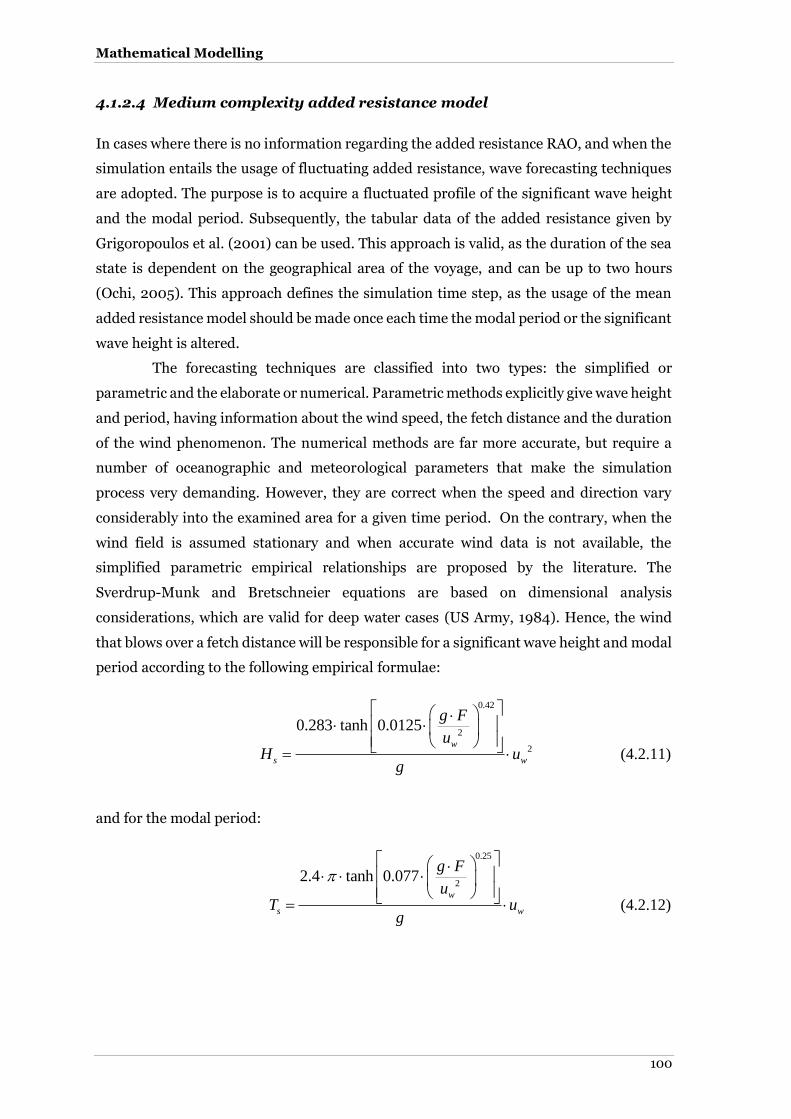
Mathematical Modelling
100
4.1.2.4 Medium complexity added resistance model
In cases where there is no information regarding the added resistance RAO, and when the
simulation entails the usage of fluctuating added resistance, wave forecasting techniques
are adopted. The purpose is to acquire a fluctuated profile of the significant wave height
and the modal period. Subsequently, the tabular data of the added resistance given by
Grigoropoulos et al. (2001) can be used. This approach is valid, as the duration of the sea
state is dependent on the geographical area of the voyage, and can be up to two hours
(Ochi, 2005). This approach defines the simulation time step, as the usage of the mean
added resistance model should be made once each time the modal period or the significant
wave height is altered.
The forecasting techniques are classified into two types: the simplified or
parametric and the elaborate or numerical. Parametric methods explicitly give wave height
and period, having information about the wind speed, the fetch distance and the duration
of the wind phenomenon. The numerical methods are far more accurate, but require a
number of oceanographic and meteorological parameters that make the simulation
process very demanding. However, they are correct when the speed and direction vary
considerably into the examined area for a given time period. On the contrary, when the
wind field is assumed stationary and when accurate wind data is not available, the
simplified parametric empirical relationships are proposed by the literature. The
Sverdrup-Munk and Bretschneier equations are based on dimensional analysis
considerations, which are valid for deep water cases (US Army, 1984). Hence, the wind
that blows over a fetch distance will be responsible for a significant wave height and modal
period according to the following empirical formulae:
0.42
2
2
0.283 tanh 0.0125w
s w
g F
uH u
g
(4.2.11)
and for the modal period:
0.25
22.4 tanh 0.077
w
s w
g F
uT u
g
(4.2.12)

Chapter 4
101
where,
g : Acceleration of gravity [m/s2]
F : Fetch [m]
uw : Wind speed [m/s]
The aforementioned formulae are valid if the duration of the phenomenon is greater than
a minimum value, which is approximated by the following equation:
0.67
2
min
68.8w
w
g F
ut u
g
(4.2.13)
In cases where the time duration of the phenomenon is less than the tmin value, equation
(4.2.13) is solved as F:
2
min0.67
68.8
w
w
u t gF
g u
(4.2.14)
Consequently, the fluctuation of added resistance due to waves is dependent on the
fluctuation of the wind speed over the examined period. Given the modal period and the
significant wave height, which are obtained by the aforementioned formulae (4.2.11) and
(4.2.12), mean added resistance data can be acquired using the tables presented in
Grigoropoulos et al. (2001).
Hydrodynamic induced forces
When the ship is sailing under favourable conditions, e.g. sea state less than 4, the ship is
experiencing lateral and yawing forces that can be neglected due to their small effect. The
rudder movement occurs only to alternate the vessel course. Nonetheless, when the ship
is sailing in sea state higher than 4, and when the relative wind direction is in a position
other than on the bow or stern, the lateral force and a yawing moment can be described by
the equations presented at the wind resistance model. According to Van Berlekom (1981),
if it is assumed that for the examined time step steady wind conditions exist, counteracting
hydrodynamic forces are induced in order to compensate the drift and yaw forces and
moments, respectively, so as to maintain the ship’s heading. These hydrodynamic forces
are expressed as a constant drift angle and a constant rudder angle.
Concerning the drift induced resistance, Van Berlekom (1981) states that Xνν
motion can be evaluated from model tests for small drift angles. The applicability of the

Mathematical Modelling
102
initial study varied for conventional tankers and bulk carriers with deadweight range of
100,000 – 500,000 tonnes (Van Berlekom et al., 1974). The aforementioned study
consisted of model tests in wind tunnels, and results in the following expression, which is
also adopted here.
2 3 210 0.1drift ppX v R L T v (4.3.1)
The lateral ship velocity (v) can be approximated by (4.3.1), that the reported speed is
always in the surge axis and the wave angle is always given relatively to the bow. Thus,
tan V (4.3.2)
Assuming that velocity at the rudder is unaffected by the propeller operation, the rudder
resistance can be expressed according to Norrbin (1972), as follows;
2 21
2Rudder RR f AR V A (4.3.3)
where,
AR : Rudder area [m2]
f(AR) : Function of rudder area which can be assumed equal to 1
δ : Rudder angle [deg]
However, this simplification implies errors in the calculation of rudder resistance.
According to Molland and Turnock (2007), the velocity in a propeller slipstream may be
made using axial momentum theory
Thus, (4.3.3) can be re-determined using the equations presented in Appendix I:
2 21
2RR RRudderR f AR V A (4.3.4)
where,
VRR : Relative rudder velocity [m/s2]
For rudders with aspect ratio 1.5-3.0, the function f (AR) equals to 1 (Van Berlekom, 1981).
The rudder angle δ is given by the following equation in a non-dimensional form:

Chapter 4
103
23
2
N Y a R
cc
C C VL
VY
(4.3.5)
where,
CN : Non-dimensional Yaw coefficient [-]
CY : Non-dimensional Sway coefficient [-]
: Displacement volume of the ship [m3]
Y’uv : Static force coefficient [-]
Y’uv δ : Vessel Hydrodynamic coefficient [-]
VR : Wind relative speed [m/s]
ξδ : N’δ/ Y’ccδ
ξβ : N’uv/ Y’uv
If the non-dimensional coefficients for the examined vessels are not known, the estimates
presented in Table 4.4 are valid for merchant ships (Van Berlekom et al., 1974; Van
Berlekom, 1981). Van Berlekom et al. (1974) proposed the following simplification of the δ
angle if no vessel hydrodynamic coefficients are known:
23
0.18 0.5 RY N
VLC C
V
(4.3.6)
Table 4.4: Static and rudder force and yawing moment coefficients estimates for merchant ships (Van Berlekom et al., 1974; Van Berlekom, 1981)
Coefficient name Coefficient value range
Y’uν -1.5 ~ -1.1
Y’ccδ 0.2 ~ 0.3
ξδ -0.5 ~ -0.4
ξβ 0.3 ~ 0.6
A similar process to account for rudder resistance when correcting the vessel heading due
to induced waves should be followed when the rudder angle is known. However, due to the
absence of reported data, the rudder added resistance movement can be neglected from
the calculation. The implied error to the total resistance determination is negligible, as the
added resistance models incorporate the rudder effect into the calculations.
Mathematical Modelling
104
Wind induced resistance
This section defines the mathematical equations that describe two statistical models of
wind resistance applicable to modern vessels. The first approach is by Isherwood (1974),
which has been proven accurate. The second by Blendermann (1994) is a more detailed
statistical correlation of data of modern hull forms. The resistance is calculated for the
surge (x-axis) movement. However, in manoeuvring condition, the movement effects in all
the vessel’s degrees of freedom are significant; nonetheless any contribution of these
factors during a sea voyage will be neglected. Nonetheless, non-dimensional coefficients
for yaw and sway movements have been approximated in order to make use of the values
at the rudder and drift resistance. It is proposed to use the Isherwood model in designs
before 1985 as the superstructure form was significantly altered after 90s; hence the
statistical analysis of Blendermann is believed to be more accurate for the modern hull
forms that this project is based on.
4.1.4.1 The Isherwood wind model
This method calculates with adequate accuracy the effect of wind in added resistance. It is
based on a statistical analysis of one hundred and seven complete model tests. It is
applicable to various hull superstructure forms for various ship types, such as tankers, bulk
carriers, cargo vessels, passenger ships and ferries, tug boats and stern trawlers. The
published paper includes a table with values of independent variables for the suggested
equations according to ship type, if vessel superstructure information is unavailable.
Although this work has full access to the design characteristics of the examined fleet, the
coupling of the project with the global fleet is possible using this approach. Thus the
equation of the x-axis force is given by:
20.5X X T RF C A V (4.4.1)
The CX coefficient is given from the multiple regression polynomial equation (4.4.2):
50 1 2 3 42 2
2 2 pOAL TX
OA OA OA
SLA A CC A A A A A A
L B B L L
(4.4.2)
where,
C : Distance from bow of centroid of lateral projected area [m]
Sp : Length of lateral projection of vessel excluding waterline, slender bodies [m]
LOA : Ship’s overall length [m]
Chapter 4
105
The non-dimensional sway coefficient is determined by:
0 1 2 32 2
4 5 6
2 2 OAL TY
OA
SS
OA OA L
LA AC B B B B
L B B
AS CB B B
L L A
(4.4.3)
The non-dimensional Yaw coefficient is given by:
0 1 2 3 4 52 2
2 2 OAL TN
OA OA OA
LA A S CC C C C C C C
L B B L L
(4.4.4)
where,
Ass : Lateral projected area of superstructure
AL : Lateral projected area of the ship [m2]
AT : Transverse projected area of the ship [m2]
4.1.4.2 The Blendermann wind model
Blendermann (1994) published a recent study for wind loads on ships using state of-the-
art methods of wind tunnel testing, and treating the data in statistical terms. The analysis
was based on twenty-eight test results, and it is accepted that they sufficiently cover
present-day ship geometries. The equations that have been suggested by Blendermann rely
on basic ship geometry characteristics. The wind force on x-axis is given by (4.4.5):
x AF FF CX q A (4.4.5)
where dynamic pressure of the apparent wind (q) is given by
20.5 wq u (4.4.6)
The coefficient CXAF is given from the following equation:
2
cos
1 1 sin 22
LAF l
F lB
t
ACX CD
A CD
CD
(4.4.7)
CDl is calculated using the linearly interpolated data of CD1AF for 0 and π angles of attack
from Blendermann (1994). Thus,
Mathematical Modelling
106
1 F
Fl A
L
ACD CD
A (4.4.8)
The non-dimensional sway coefficient is determined by:
2
1
sin
1 1 sin 22
Y T
B
T
C CDCD
CD
(4.4.9)
The non-dimensional Yaw coefficient is given by:
0.182
LN Y
OA
SC C
L
(4.4.10)
where,
ε : Wind angle of attack [rad]
δΒ : Cross-force parameter [0-1]
SL : Position of the lateral-plane centroid with respect to the main section [m]
The Propulsor and Governor models
The behaviour of the machinery operation is defined by requirements in torque and
rotational speed. Journee (1976) states that the relation of the engine speed at constant
setting and the increased loading in a seaway is also important. As a result, the
mathematical implementation of the forces acting on the ship due to the operation of the
propeller is necessary and the coupling between the propeller operation and engine is
essential.
4.1.5.1 The Propeller model
The main force that the propeller produces is the thrust, which is always along the x-axis.
Apart from the thrust, another interesting expression of the propeller’s operation is the
torque acting on the main shaft. In practical terms, part of the force due to propeller-hull
hydrodynamic interaction is lost. The percentage of this coefficient is dependent on the
geometry of the hull and the appendages. This is expressed through the thrust-deduction
factor t and the propeller force is given by:
0 1T T t (4.5.1)

Chapter 4
107
In order to have a self-propelled ship (sum of forces equal to zero), T should be equal to
the total ship resistance (RT). Thus by taking into account the thrust deduction due non
open water propeller conditions:
01
TRT
t
(4.5.2)
where,
T0 : Open water developed thrust [N]
t : Thrust deduction factor [-]
The method that was followed by Oosterveld and Oossanen (1975) to calculate the
thrust and torque is based on the Wageningen B-screw series data. The open-water
characteristics are obtained from open-water test results, for about one hundred and
twenty propellers. They are given in a conventional way, in the form of thrust and torque
coefficients KT and KQ, respectively. However, if detailed propeller model tests are
available, the following equations (4.5.3) - (4.5.5) should not be used and the non-
dimensional thrust and Torque coefficients are supplied directly by the KT, KQ, and η0
graph. In the case of the Wageningen B-screw series:
0
2 4T
w p
TK
n D
(4.5.3)
0
2 5Q
w p
QK
n D
(4.5.4)
where,
n : Propeller revolutions per second [rps]
Dp : Propeller diameter [m]
Q0 : Open water developed torque [Nm]
In order to calculate the thrust and the torque, coefficients should be defined. Oosterveld
and Oossanen (1975) have published a polynomial form of the coefficients using non-
dimensional propeller data, such as the number of blades, the expanded blade ratio, the
pitch to diameter ratio and the advance coefficient. The polynomials in the following
equations are valid for Reynolds number, Re=2x10⁶ at 75% of the propeller radius.

Mathematical Modelling
108
39
01
47
01
/ /
/ /
n nn n
n nn n
t us vn pT E
n
t us vn p EQ
n
K C J P D A A z
K C J P D A A z
(4.5.5)
where,
Cn, Sn, un, vn are coefficients determined in (Oosterveld and Oossanen, 1975)
J : Advance speed and given by equation (3.57)
Z : Number of blades
The advance speed is given by:
A
p
VJ
n D
(4.5.6)
Where VA is the advance velocity given by:
1A
V V w (4.5.7)
In order to determine the KT and KQ coefficients for other than Reynolds number equal to
2x10⁶, corrections have to be made as described in Oosterveld and Oossanen (1975).
The shaft horsepower (SHP) in kW required by the prime mover is given by
equation (4.5.8)
3 2 510 2Q w p
tr R
K n D nP
(4.5.8)
where,
ηtr : Shaft losses between the prime mover and the propulsor [-]
ηR : Relative rotative efficiency [-]
w : Wake friction [-]

Chapter 4
109
4.1.5.2 The Governor and Bridge Commands models
The purpose of the Engine Governor is to regulate the fuel consumption so to maintain a
predefined engine speed. In Diesel Engines, due to the excess air that is always present in
combustion, the consumption without the presence of the governor would increase and
the engine speed would not have a limit. As a result, in order to control the engine speed,
a governor regulates the injected fuel (Woodyard, 2009). Consequently, the regulation of
fuel and engine speed defines the ship’s speed, as the available power to the propulsor is
controlled.
The coupling of the propeller is defined mathematically by the following
principle: in the case of desired vessel speed, the torque needed by the propeller must be
in equilibrium with the engine delivered torque and the thrust delivered by the propeller
must be in equilibrium with the total resistance of the ship (Molland et al, 2012: Journee,
1976). As a result, the rotational speed of the propeller is defined by equalising the
developed thrust with the total ship resistance. According to the three-parameter theorem
(Politis, 1991), when there is information regarding the propeller and its operation, the
remaining information can be determined using the KT, KQ graph. In the propulsion
problem, the thrust, the propeller diameter and the desired vessel speed are known. Thus,
the revolutions per second and the power requirement are defined. In the simulation, the
determination of the propeller rotational speed was found by the trial and error method,
which was optimised using numerical analysis techniques (midpoint method) with a
tolerance equal to 10-7. The determination of engine speed and power can be characterised
as an engine governor.
The different application of the simulated engine governor is to maintain constant
power. The controller is now responsible for altering the engine speed in order to meet the
constant power setting when the total ship resistance changes due to added resistance,
imposed by wind and waves. In terms of simulation modelling, the method adopted in the
simulator is trial and error. The algorithm is altering the vessel speed until it reaches the
defined power setting with respect to the resistance thrust equilibrium. The resistance
thrust match is different in each trial step, since the resistance component is mainly
dependent on the vessel speed and has a unique power requirement.

Mathematical Modelling
110
Main Engine simple model
The Diesel engine was modelled using the manufacturer’s engine operational maps. The
acquired data provided information for the complete engine operation, in terms of
temperatures, pressures, turbocharger operation, power-RPM curves for normal loading
and specific fuel oil consumption versus power output. The latter value is corrected
according to the manufacturer. Due to the existence of lube oil pumps, different than ISO
conditions in air temperature and cooling water temperature, the SFOC is increased.
Furthermore, the HFO operation of lower calorific value significantly alters the SFOC
(MAN Diesel, 2007). Thus, the following corrections should be made:
There is a 0.6% increase in fuel consumption due to different than ISO inlet temperature
for every 10oC:
4
1 6 10CR T (4.6.1)
For different lower calorific value fuel (Θu ≠ 42700kJ/Kg):
2
427001
u
CR
(4.6.2)
For marine gas oil (MGO) consumption:
30.02CR (4.6.3)
For lube oil pump operation, the losses leading to CR4 are dependent on engine load.
Hence,
4
corrected ISO
1
1 iSFOC SFOC CR
(4.6.4)
The equations outlined above must be combined with the engine efficiency curves, which
were presented in Figures 3.15 and 3.16.
Miscellaneous calculations
This section covers mathematic transformations and coefficient calculations that are
present on the developed simulation block library.
The kinematic viscosity and water density respectively are given by:
3
2 9
1.023379273 0.001787 10
1 33.408772 0.1681570669 10sw
w wT T
(4.7.1)

Chapter 4
111
2 30.48033168167 7.6223076145 10 104.83sw w wT T g (4.7.2)
where,
TW : Water temperature [C]
g : Acceleration of gravity [m/s]
Tair : Air temperature [C]
The air density is given by:
1.00336360.7782air airT (4.7.3)
The wake, thrust deduction and relative rotation propulsion coefficients are
essential for calculation. The thrust deduction factor is approximated using the following
the expressions of Holtrop and Mennen (1981) and SSPA laboratory, which have better
accuracy versus the actual coefficients of other approximations found in the literature.
For single screw cargo vessels:
0.26840.28956
0.01762
0.25014
0.00151 0.0225
stern
P
B B T
L Dt C
C lcb
(4.7.4)
1.57 2.3 1.5BB
WP
Ct w C
C
(4.7.5)
The wake coefficient is approximated by Holtrop and Mennen (1981) and Kruger (1976),
respectively.
For single screw cargo vessels:
0.3 10 0.1B V B
w C C C (4.7.6)
0.75 0.24B
w C (4.7.7)
The relative rotation efficiency is calculated by the formula proposed by Holtrop and
Mennen (1981).

Mathematical Modelling
112
For single screw cargo vessels:
0
0.9922 0.05908 0.07424 0.0225ER P
AC lcb
A (4.7.8)
where,
D : Ship’s Drought [m]
CP : Prismatic coefficient [-]
CB : Block coefficient [-]
CWP : Water plane coefficient [-]
Cstern : Stern type as described in Holtrop and Mennen (1981) [-]
lcb : Longitudinal centre of buoyancy expressed in percentage from amidships [%]
AE/A0 : Propeller expanded blade area ratio [-]
P/D : Propeller pitch to diameter ratio [-]
Generation of environmental parameters
The wind speed changes continuously and, in order to obtain long-term estimations,
statistical methods are used. In marine applications these areas can be sea areas of large
fetch distance and can be described by geographical coordinates. Hatziargyriou et al.
(1993) state that the Weibull probability density function has been widely used to describe
variations of wind speed for an examined area. The Weibul model is given by the following
relationship:
1
a
wua
w wa uf V e
(4.8.1)
where,
uw : wind speed [m/s]
a : shape factor of Weibul probability density function [-]
b : scale factor of Weibul probability density function [-]
a, β coefficients can be obtained using the following two expressions:
0
11w w w
w
u u f u dva
(4.8.2)
where,
Chapter 4
113
Γ : Gamma function
The variance of the wind measurements is given by:
2 2 2
0
2 11 1w w w
w w
u u f u dva a
(4.8.3)
The mean wind speed value is given by (4.8.4):
1
1 N
w wi
i
u uN
(4.8.4)
where,
N : Total number of wind speed measurements [-]
The standard deviation (σ) can be found using:
2
1
1 N
wi w
i
u uN
(4.8.5)
Equations (4.8.2) and (4.8.3) can be solved simultaneously to obtain a, β coefficients.
However, this process is considered complex and slow, hence the Justus (1978) approach
is used, which defines a as:
1.086
ww
au
(4.8.6)
Thus, the β coefficient can be obtained using (4.8.2).
Hatziargyriou et al. (1993) also proposed a random generation wind model using
the Weibul coefficients obtained from the long-term statistical model. The inverse
transformed method consists of:
1
awwu
RF V e
(4.8.7)
Solving (4.8.7) for R, the pseudo-random number generator is defined:

Mathematical Modelling
114
1
1ln 1 wa
wF R R u (4.8.8)
The Rayleigh distribution is a simplified version of the Weibul distribution. It is globally
accepted that a Normal distribution can accurately describe the wind direction, given the
mean angle value and the standard deviation.
For the approximation of the Wind velocity, the α coefficient of the Rayleigh
distribution should be defined. Usually, in a vessel noon report, only the mean relative
wind speed is reported. Thus, using a Rayleigh random number generator, a statistical
sample of N values can be acquired. Hence,
2
Ww
ua
(4.8.9)
A third model, which is suitable for application in a ship simulator, is defined by
Anderson et al. (1983). This model can properly simulate the spatial effect of wind
behaviour, including gusting, rapid changes and background noises. Consequently, the
wind model is a four-component model and is given by the following equation:
M WB WG WR WNV V V V V (4.8.10)
The mathematical equation set of the (4.8.10) wind model subcomponents is given in
Appendix I.
Chapter 4
115
4.2 Energy storage system
More than 90% of the world’s fleet is powered by Diesel Engines. The majority of ocean-
going ships are propelled by a two-stroke slow speed Diesel Engine directly coupled to the
propulsion shaft. In high Froude number vessels, the propulsion system is broken down
into multiple four-stroke Diesel Engines or into multiple Diesel Generator sets, which
power electric motors that are coupled to the propeller shaft(s) (Klein Wood and
Stapersma, 2003; Bose, 2008).
The hybrid module, as discussed in the previous chapters, consists of a specific
number of battery banks that fulfil two basic requirements. The first is battery voltage,
which is constrained by the battery manufacturer, and the second is the required Capacity,
as found in Table 3.4. In this study, the battery banks are treated as a one, formed by the
appropriate number of strings and parallel units.
4.2.1 Sizing of battery banks
The energy storage system capacity is determined by the vessel type and autonomy radius
of the ship, as it was estimated by correlation of voyage energy requirements. The required
voltage is determined by the designer and is constrained by the transformer capability of
altering voltage. Usually, the propulsion system runs from 0.4 – 13.8kV and alternations
of the voltage are determined by the on-board applications, which can be 220V for hotel
loads, 380V for auxiliary equipment and, dependent on the motor type, up to 1kV for
propulsion.
The total number of batteries (nbs) that should be connected in series in order to
implement one battery string is dictated by the DC-bus voltage (Vop) and the nominal
battery voltage (Vbat). The DC-bus nominal voltage is equal to the DC/AC converter DC
input nominal voltage (Koutroulis et al., 2009). Thus,
op
bs
bat
Vn
V (4.9.1)
The total nominal capacity (Cnom) of the battery bank [MWh], Qnom depends on the nominal
capacity of each battery Qbatmax (Ah) and the total number of strings forming the battery
bank (NBB). Hence,
maxnom BB batC N Q (4.9.2)
The battery manufacturer denotes that sixteen parallel units of Sodium Nickel Chloride
can be connected, offering a nominal voltage of 557V and 0.285 MWh energy density.

Mathematical Modelling
116
Transforming equation (4.9.2) and by constraining the result (value has to be rounded to
the next integer), the number of the Battery Banks is given by:
.Energy
0.285
req
BBN (4.9.3)
In addition, given that the discharge/charge current is one of the most important
parameters of battery efficiency, the current should remain as low as possible. In testing
facilities, these sixteen parallel units that form a large battery bank offer 0.5MW maximum
power. Moreover, with the appropriate connections and converters, multiple banks can be
connected, increasing the energy storage medium capability. Hence, due to the parallel
connection of the batteries, the discharge/charge current is found using the following
relationship:
demand
nominaldischarge/ Charge
16BB
P
VI
N
(4.9.4)
where,
Pdemand : Demanded power by the propulsion and/ or auxiliary loads [W]
Vnominal : Battery Nominal Voltage [V]
NBB : Number of Battery Banks [-]
However, the total number of DC/AC converters (Nc) required to implement the Hybrid
system is calculated by the guaranteed power value (PG) and the nominal AC power rating
of the selected converter. Consequently,
0
0
GC
F PN
P
(4.9.5)
where,
Fo : Oversizing factor and is determined by the designer.

Chapter 4
117
4.2.2 Battery models
This thesis proposes the use of two models that sufficiently describe battery behaviour.
The experimental model requires laboratory measurements that are often not available to
the designer. The second model is a modified version for a quasi-steady condition dynamic
model for the battery operation. This model requires significantly less information
regarding the battery type. However, the battery coefficients are available in the literature
for a range of commercial batteries.
4.2.2.1 Battery experimental model
The model makes use of the information provided by the manufacturer (Manzoni et al.,
2008). Detailed efficiency calculations had been presented in Chapter 3. The following
equation is used to estimate the available energy in the battery per simulation time step.
2
OC OC
t
nom oc nom oc
V i i R t V i dV i tSoC
Q V Q V
(4.9.6)
For the charging and discharging efficiencies, respectively:
2
.
OC OC
ch
oc oc
V i i R V i dV i
V i V i
(4.9.7)
. 2
OC OC
dis
OCOC
V i V i
V i dV iV i i R
(4.9.8)
Using (4.9.6) and (4.9.7), Figures 3.12 and 3.13 are constructed.
where,
VOC : Open circuit voltage [V]
i : battery current [A]
dV : Voltage drop [V]

Mathematical Modelling
118
4.2.2.2 Kinetic Battery Model
The Kinetic batery model (KiBaM) model is called kinetic because the approach is
developed on the basis of a chemical kinetics process (Manwell et al., 2005). Although this
model is dynamic, it can be transformed to a quasi-steady model under appropriate
conditions. The model of the battery charge is distributed in two wells. The first well is the
available-charge and the second is the bound-charge. The first describes the available
energy ready for system supply. The second determines the amount of energy that is
processed in order to fill the available energy well. The rate at which charge flows between
the wells depends on the difference of height of the two wells, defined by parameter k.
Parameter c gives the fraction of the total charge in the battery that is part of the available-
charge well (Manwell et al., 2005). The procedure is described by two differential
equations (4.9.9) and (4.9.10).
12 1
dyI k h h
dt (4.9.9)
22 1
dyk h h
dt (4.9.10)
The initial conditions are:
1 max
2 max
0
0 1
KB
KB
y c Q
y c Q
(4.9.11)
The solution is given by applying Laplace transformation (4.9.12-4.9.13)
0
1 1,0
1 1k t k t
k ty k c I e I c k t e
y y ek k
(4.9.12)
2 2,0 0
1 11 1
k t
k t k tI c k t e
y y e y c ek
(4.9.13)
where
yi,0 is the amount of available and bound charge respectively at the start of each time step.
For t=0 the values are equal to the initial conditions of the problem.
k’ is defined as
1
kk
c c
(4.9.14)
In the energy approach of the Hybrid system, however, the demand of electrical
power and energy from the batteries is described by Power and Capacity and not by

Chapter 4
119
current. Hence, equations (4.9.12), (4.9.13) can be transformed to energy by being
multiplied by the Voltage (Vrettos and Papathanassiou, 2011). If the voltage curve is not
known, it can be assumed as constant until a specific state of charge (SoC) is reached.
However, this procedure introduces errors, as it does not take into account the different
charge or discharge currents. Nonetheless, a proper sizing and a charge-discharge
controller could apply constant current to the battery arrays without affecting the
performance of either the battery or the model.
0
1 1,0
1 1k t k t
k tE k c P e P c k t e
E E ek k
(4.9.15)
2 2,0 0
1 11 1
k t
k t k tP c k t e
E E e E c ek
(4.9.16)
The KiBaM approach offers a voltage model. However, in order to apply curve fitting and
to export a curve that depicts the voltage drop versus current (Manwell et al., 2005), it
requires experimental data from the battery.
OC
XV V A X C
D X
(4.9.17)
Where, the A coefficient is a parameter reflecting the initial linear variation of internal
battery voltage with state of charge. Typically, it is negative when discharging and positive
when charging. C is a parameter that reflects the decrease/increase of voltage when
batteries are progressively discharged/charged. It is negative when discharging and
positive when charging. D is a parameter reflecting the decrease/increase of battery
voltage when the battery is progressively discharged/charged. D is positive and is normally
approximately equal to the maximum capacity. However, the nature of the fitting process
will usually be such that it will not be exactly equal to that value.
X is a normalised maximum capacity at the given current and is defined as follows:
max
qX
Q (4.9.18)
and for discharging X is defined as:
max
max
Q qX
Q
(4.9.19)

Mathematical Modelling
120
The percentage of the energy that the Hybrid system can absorb or give to the energy
storage medium is dependent on the excess or lack of the propulsion energy requirement
in every time step. Thus,
demanddemand
PI
V (4.9.20)
excessexcess
PI
V (4.9.21)
In order to check that the storage medium has sufficient energy to export/import to and
from the Hybrid system, the maximum discharging/charging current has to be calculated.
As a result,
1,0 0
,max
1
1 1
k t k t
demand k t k t
k q e q k c eI
e c k t e
(4.9.22)
max 1
charging,max
1
1 1
k t
k t k t
k c Q k q c eI
e c k t e
(4.9.23)
The energy equations can be found by multiplying constant Voltage with equations
(4.9.22) and (4.9.23), which that introduces error to the calculations, as previously
explained.
According to the kinetic battery model approach, the capacity of the battery is
preserved and any losses during charging/discharging are caused by the voltage change
during these phenomena. In order to calculate the losses, the voltage at each time step is
compared to the nominal voltage of the battery. The value of battery voltage can be found
if the current and State of Charge (SoC) are known. When battery capacity is almost
depleted (Depth of discharge ~100%), the current is ~0A, thus the battery voltage is equal
to the E of the empty battery. During charge, when the battery reaches its nominal
capacity, the current is high and the terminal voltage is different than battery’s E, hence
the losses are high. The losses are given by the equation (4.9.24):
( , )ch nomL I V I t V (4.9.24)
In cases where actual experimental data or manufacturer curves of the battery are not
available, equation (3.25) is not used. Consequently, in order to take into account the
energy losses, the round-trip efficiency can be used instead.

Chapter 4
121
4.3 Optimisation of Machinery Operation
The hybrid configuration implies the existence of an energy management strategy that will
choose the optimum power split between the operation of combustion engines and the
usage of electricity drained out of the batteries. The strategy is developed to achieve system
level objectives, such as fuel economy, low emissions of CO2 and particulate matter, and
battery charge sustenance. According to Xu et al. (2010), the energy management
strategies can be classified into two categories: the rule-based, in combination with fuzzy
logic control if applicable (Schouten et al., 2002), and the optimal. A rule-based strategy
is feasible and can be implemented in real time application based on heuristic methods.
The optimal strategies differ from each other in each time step, e.g. the fuel consumption
is minimised during this time step. A more global solution can be extracted using Dynamic
Programming (DP), which relies on the principle of optimality, where the optimal policy
can be built step by step. This can be achieved by building an optimal control of the tail
sub-problem. It involves the last step and then progresses it towards the front time series
steps by iterating and by involving the last two stages during each control (Rousseau et al.,
2008). For automotive applications, Lin et al. (2001) and Musardo et al. (2005) proposed
the usage of DP, which is well suited to multistage processes, instead of the fuzzy based
approach. Nevertheless, the problem with the application of DP is that the operational
profile of the vessel is not known in advance, as the chartering commands may alter the
speed or, due to unexpected weather change, the forecasted situations may not be
encountered during the voyage. In addition, if the vessel operates at constant speed, it is
not possible to acquire a-priori the propulsor loading, because sea behaviour is stochastic.
In literature, two implementations for describing the power train in combination with the
operator commands are found. The forward facing implementation has as an input the
desired propulsive power, thus the M/E provides the equivalent torque to the propeller
and the vessel speed is subsequently determined. This approach is more complex than the
backward facing model. The latter approach uses a speed profile (in the marine case, the
master speed command), and afterwards the model calculates backward the
corresponding operating point of the M/E (Musardo et al., 2005). The backward approach
is selected and is also proposed by Van Kessel (2007) for the simulation of submarine
battery operation. Thus, the energy strategy has to anticipate a future power demand at
the next simulation time step (Grimmelius et al., 2011). To deal with this problem, Guzzella
and Sciarretta (2005) proposed the implementation of a cost function in combination with
the optimisation routine. ECMS treats the combustion engines as prime cost factors, while
the energy storage system is a secondary cost factor, which costs fuel in the future but is
inserted into the optimisation algorithm in the examined step. Moreover, during charging,

Mathematical Modelling
122
the cost of fuel to charge is reduced from the fuel bill because this will eventually save fuel
in the future. This approach involves a comparison of charging and discharging solutions,
and the optimal one is the minimum of the two. This approach was adopted and
implemented in this project. However, a different pseudo multi-objective optimisation is
also given for reduction of not only of CO2 but of PM. The second approach will be
described firstly in this chapter as it is more complex than the ECMS.
The optimisation algorithm selected in this study is a non-linear medium scale
optimisation algorithm based on a sequential programming method (Hock and
Schittkowski, 1983; Fiacco and Mc Cormick, 1990), which updates the Hessian of the
Lagrangian by applying the Broyden, Fletcjer, Goldfarm and Shanno (BFGS) method
(Shanno, 1985). It is a single objective optimisation, where the selection of the objective
function in all stages of a ship’s voyage is the fuel consumption. This optimisation
algorithm was selected between the Trust region reflective, active set and internal point
algorithms. These algorithms are also proposed by Mathworks® for solving that type
optimisation problems. The main reasons for this adoption are that this algorithm
converges rapidly to the optimal solution, identifies rapidly the local minima and given the
different start points it converges to the global minimum, while active set for example fails.
The algorithm principles and the programming process are presented in Nocedal and
Wright (2006).
For each of the Hybrid Power layouts, an objective function was formed and the
linear and non-linear constraints (equalities and inequalities) were implemented. The set
of equations is separated into two parts because of the fact that, due to layout constraints,
the electric machine can operate either as an electric motor, hence boosting the propulsion,
or act as a shaft generator, thus absorbing energy from the two-stroke Diesel engine in
loads more than 60% of maximum continuous rating (MCR) and producing electricity.
Concerning the global restrictions applied to each scenario, the following variable limits
have been employed. The shape of the objective function has great influence on the
successful identification of the global minimum solution. The non-convex form of the
objective function has many local minima. To guarantee that the solution is for the global
minimum, a commonly suggested method is to change the starting value vector and re-run
the optimisation in order to skip each time the already identified solution of this local
minimum. Once this process is made several times, where the number is denoted by the
degree of the polynomial objective function (e.g. it is a polynomial of n degree, then the
local minima can be up to n-1), the outputs are compared and the minimum is the global
minimum solution.
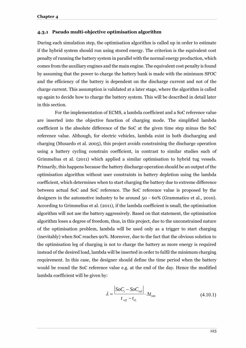
Chapter 4
123
4.3.1 Pseudo multi-objective optimisation algorithm
During each simulation step, the optimisation algorithm is called up in order to estimate
if the hybrid system should run using stored energy. The criterion is the equivalent cost
penalty of running the battery system in parallel with the normal energy production, which
comes from the auxiliary engines and the main engine. The equivalent cost penalty is found
by assuming that the power to charge the battery bank is made with the minimum SFOC
and the efficiency of the battery is dependent on the discharge current and not of the
charge current. This assumption is validated at a later stage, where the algorithm is called
up again to decide how to charge the battery system. This will be described in detail later
in this section.
For the implementation of ECMS, a lambda coefficient and a SoC reference value
are inserted into the objective function of charging mode. The simplified lambda
coefficient is the absolute difference of the SoC at the given time step minus the SoC
reference value. Although, for electric vehicles, lambda exist in both discharging and
charging (Musardo et al. 2005), this project avoids constraining the discharge operation
using a battery cycling constrain coefficient, in contrast to similar studies such of
Grimmelius et al. (2011) which applied a similar optimisation to hybrid tug vessels.
Primarily, this happens because the battery discharge operation should be an output of the
optimisation algorithm without user constraints in battery depletion using the lambda
coefficient, which determines when to start charging the battery due to extreme difference
between actual SoC and SoC reference. The SoC reference value is proposed by the
designers in the automotive industry to be around 50 - 60% (Grammatico et al., 2010).
According to Grimmelius et al. (2011), if the lambda coefficient is small, the optimisation
algorithm will not use the battery aggressively. Based on that statement, the optimisation
algorithm loses a degree of freedom, thus, in this project, due to the unconstrained nature
of the optimisation problem, lambda will be used only as a trigger to start charging
(inevitably) when SoC reaches 90%. Moreover, due to the fact that the obvious solution to
the optimisation leg of charging is not to charge the battery as more energy is required
instead of the desired load, lambda will be inserted in order to fulfil the minimum charging
requirement. In this case, the designer should define the time period when the battery
would be round the SoC reference value e.g. at the end of the day. Hence the modified
lambda coefficient will be given by:
.
t ref
sim
ref el
SoC SoCt
t t
(4.10.1)

Mathematical Modelling
124
where,
SoCt : Battery State of Charge at simulation time t [%]
SoCref : Reference Battery State of Charge, user defined [%]
tref : Reference time where the SoCt must be equal to SoCref [h]
tref : Simulation elapsed time [h]
Δtsim : Simulation time step [h]
Based on equation (4.10.1), it can be extracted that when the simulation time approaches
the time reference value, the charging will be more aggressive than in early simulation
steps. When simulation time exceeds the reference value, the tel. variable is set again to
zero and the process is restarted. Although, this equation maintains the SoC at the desired
level, it is not guaranteed that the charging occurred in an optimum manner. To solve this
problem, instead of producing a Dynamic Programming Code, as no future loading is 100%
known in advance, the following propositions are made:
If the battery SoC is not equal to zero, it is different than the SoCref and at the
current simulation step the Pbat = 0 based on the optimisation algorithm, the following
criteria are applied:
a) Constrain charging if charging current is more than 5A. It can be extracted from
Figure 3.13 that charging efficiency drops significantly in high charging currents.
b) In layouts B and C charging is not possible if engine speed is less than 60% of the
nominal value.
c) The optimisation objective should be changed to operate the engine with the
minimum SFOC. This requirement leads to a pseudo-multivariable optimisation
problem, where, in particular cases, the two objectives are transformed again into
a single objective problem, which is the SFOCmin instead of the minf. When
applying that type of optimisation, a set of assumptions and project-defined
solutions should be applied. Firstly, the optimisation algorithm is programmed to
identify the number of engines operating at low non-zero loads. It also counts the
number of engines that operate at the same low load. Moreover, the algorithm is
programmed to divide the equivalent extra loading by the number of generators, in
order to increase the load of each of these engines into higher efficiency points. The
SFOCmin algorithm is driven by the fact that a parallel goal of this study is to reduce
exhaust emissions. By increasing the load of the engines, the amount of Particulate
Matter is reduced (Wright, 2000).
d) In cases where engine is loaded at a percentage higher than its optimum value, the
c) criterion is not valid, since the engine needs to reduce the load to meet the
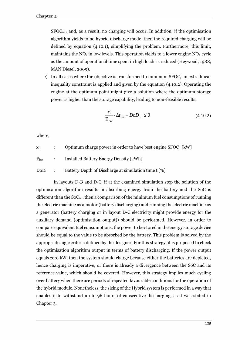
Chapter 4
125
SFOCmin and, as a result, no charging will occur. In addition, if the optimisation
algorithm yields to no hybrid discharge mode, then the required charging will be
defined by equation (4.10.1), simplifying the problem. Furthermore, this limit,
maintains the NOx in low levels. This operation yields to a lower engine NOx cycle
as the amount of operational time spent in high loads is reduced (Heywood, 1988;
MAN Diesel, 2009).
e) In all cases where the objective is transformed to minimum SFOC, an extra linear
inequality constraint is applied and given by the equation (4.10.2). Operating the
engine at the optimum point might give a solution where the optimum storage
power is higher than the storage capability, leading to non-feasible results.
1 0E
isim t
Bat
xt DoD (4.10.2)
where,
xi : Optimum charge power in order to have best engine SFOC [kW]
Ebat : Installed Battery Energy Density [kWh]
DoDt : Battery Depth of Discharge at simulation time t [%]
In layouts D-B and D-C, if at the examined simulation step the solution of the
optimisation algorithm results in absorbing energy from the battery and the SoC is
different than the SoCref, then a comparison of the minimum fuel consumptions of running
the electric machine as a motor (battery discharging) and running the electric machine as
a generator (battery charging or in layout D-C electricity might provide energy for the
auxiliary demand (optimisation output)) should be performed. However, in order to
compare equivalent fuel consumptions, the power to be stored in the energy storage device
should be equal to the value to be absorbed by the battery. This problem is solved by the
appropriate logic criteria defined by the designer. For this strategy, it is proposed to check
the optimisation algorithm output in terms of battery discharging. If the power output
equals zero kW, then the system should charge because either the batteries are depleted,
hence charging is imperative, or there is already a divergence between the SoC and its
reference value, which should be covered. However, this strategy implies much cycling
over battery when there are periods of repeated favourable conditions for the operation of
the hybrid module. Nonetheless, the sizing of the Hybrid system is performed in a way that
enables it to withstand up to 96 hours of consecutive discharging, as it was stated in
Chapter 3.
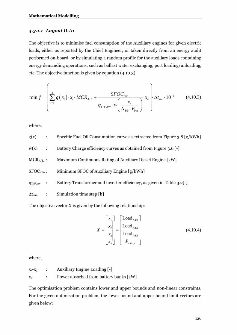
Mathematical Modelling
126
4.3.1.1 Layout D-A1
The objective is to minimise fuel consumption of the Auxiliary engines for given electric
loads, either as reported by the Chief Engineer, or taken directly from an energy audit
performed on-board, or by simulating a random profile for the auxiliary loads containing
energy demanding operations, such as ballast water exchanging, port loading/unloading,
etc. The objective function is given by equation (4.10.3).
3
6min/ 4
1 4/ ,
min 10i i A E sim
i
T F inv
BB bat
SFOCf g x x MCR x t
xw
N V
(4.10.3)
where,
g(x) : Specific Fuel Oil Consumption curve as extracted from Figure 3.8 [g/kWh]
w(x) : Battery Charge efficiency curves as obtained from Figure 3.6 [-]
MCRA/E : Maximum Continuous Rating of Auxiliary Diesel Engine [kW]
SFOCmin : Minimum SFOC of Auxiliary Engine [g/kWh]
ηT/F,inv : Battery Transformer and inverter efficiency, as given in Table 3.2[-]
Δtsim : Simulation time step [h]
The objective vector X is given by the following relationship:
A/E11
A/E22
A/E33
4
Load
Load
Load
battery
x
xX
x
Px
(4.10.4)
where,
x1-x3 : Auxiliary Engine Loading [-]
x4 : Power absorbed from battery banks [kW]
The optimisation problem contains lower and upper bounds and non-linear constraints.
For the given optimisation problem, the lower bound and upper bound limit vectors are
given below:
Chapter 4
127
0 0 0 0lb (4.10.5)
cap.
1
Bat1 1 1 1
t
sim
ub DoDt
(4.10.6)
where,
DoDt-1 : Battery Depth of Discharge at previous time step [%]
Batcap : Battery Energy Capacity, defined at the design stage or by Table 3.8 [kWh]
This non-linear optimisation problem has a linear inequality for the discharge current. The
linear inequality has to be in the following form:
AX b (4.10.7)
Thus,
4 . .
1max
16d c
BB Bat
xN V
(4.10.8)
where,
VBat : Battery Voltage [V]
Maxd.c. : Battery Maximum Discharge current, as presented in Figure 3.5 [A]
The non-linear equality regarding how the hybrid system will meet the power
requirements is given by the following equation:
3
.4/ / , 4
1
req
i A E gen T F inv
i BB Bat loss
Pxx MCR w x
N V
(4.10.9)
where,
ηgen : Auxiliary Engine generator efficiency, as given in Table 3.2 [-]
ηloss : Transmission losses, as given in Table 3.2 [-]
Preq. : Required Power [kW]
For the charging scenario, the number of running generators is known in advance. The
algorithm selects the number of the worst loaded engines and increases their load in order

Mathematical Modelling
128
to minimise their specific fuel oil consumption. Hence, the following non-linear
optimisation constraint has to be satisfied by the process:
3
.4/ / , 2 4
1
req
i A E gen T F inv
i BB Bat loss
Pxx MCR w x
N V
(4.10.10)
4.3.1.2 Layout D-A2
The only difference between Layout D-A1 and Layout D-A2 is that Layout D-A2 will
probably not have identical generator sets. Based on the preliminary study that was
described in Chapter 3, the principle of switching generator sets on and off and running
them at near optimum loading points covering all the demands of the vessel, is investigated
by this optimisation algorithm. Based on the initial analysis, two types of Diesel Generator
Sets will be used. Consequently, the optimisation algorithm of D-A1 layout is altered in
specific parts. The equations describing this system are given bellow:
/ 1 / 2
1 1
6
min4
4/ ,
min 10
n m
i i A E i A E
i i
sim
T F inv loss
BB Bat
g x x MCR h x x MCR
SFOCf tx
xw
N V
(4.10.11)
where,
g(x) : Specific Fuel Oil Consumption curve for type I Diesel Generator Set
obtained from the manufacturer [g/kWh]
h(x) : Specific Fuel Oil Consumption curve for type II Diesel Generator Set
obtained from the manufacturer [g/kWh]
The non-linear equality constraint that defines how the hybrid system will meet the power
requirements is given by the following equation:
/ /
1 1
.1/ , 1
. / .
n m
i A E I gen I i A E II gen II
i i
reqn mT F inv n m
BB Bat m prd loss T F Conv
x MCR x MCR
Pxw x
N V P
(4.10.12)
Chapter 4
129
For the charging scenario, the (4.10.12) is transformed to:
/ /
1 1
.1/ , 1
. / .
n m
i A E I gen I i A E II gen II
i i
reqn mT F inv n m
BB Bat m prd T F loss Conv
x MCR x MCR
Pxw x
N V P
(4.10.13)
where,
Preq. : Required Power [kW]
Pprd. : Produced Power [kW]
ηm : Electric motor efficiency curve, as depicted in Figure 3.7 or supplied by the
motor manufacturer
ηT/F : Propulsion motor transformer efficiency, as given in Table 3.2[-]
ηconv. : Propulsion converter efficiency, as given in Table 3.2 [-]
4.3.1.3 Layout D-B
This layout describes a Hybrid system where the existence of the battery aids only the main
propulsion. The electricity is supplied to an electric motor, which is coupled to a gearbox-
clutch. This motor provides the extra power for the propulsion when needed. Charging
occurs only when the electric machine operates as a generator. In order for the latter to
operate as a generator, constraints apply as described previously. In the simulation, the
voyage phase is a user input. In this case, the controller understands how to treat the
hybrid system. Moreover, in every simulation time step, the propulsion power is divided
by the engine MCR, in order to define the initial operational point of the engine, thus
deciding which optimisation algorithm to apply. The objective is to minimise fuel
consumption. Hence the objective function is given by equation (4.10.14).
1 1 /
6
min2
/ , . 2 2
min 10
M E
sim
T F inv loss g conv m
d x x MCR
f tSFOCx
x w x
(4.10.14)
The optimisation vector X is given by the following relationship:
M/E1
2
Load
battery
XX
PX
(4.10.15)

Mathematical Modelling
130
where,
x1 : Main Engine Loading [-]
x2 : Power absorbed from battery banks [kW]
The optimisation problem contains lower and upper bounds and non-linear
constraints. For the given optimisation problem, the lower bound and upper bound limit
vectors are given below:
0 0lb (4.10.16)
1 cap.min , 1 Bat
m tub p rpm MCR DoD
(4.10.17)
Layout D-B has the same constraints as described by equations (4.10.7) - (4.10.8).
The non-linear equality regarding on how the hybrid system will meet the power
requirements is given by the following equation (4.10.18):
/ 1 / / , 2 2 2 .g M E C T F loss T F inv m reqMCR x x w x x P (4.10.18)
Although equations (4.10.14) - (4.10.18) outline the hybrid controller behaviour
for the main propulsion when the electric machine operates as a motor, for the majority of
the operational period, due to conversion losses, the system is running as a shaft generator,
hence the electric machine acts as generator and the batteries are either charging, or are
decoupled from the system and the propulsion machinery behaves conventionally. The
optimisation objective is once again changed to that of minimum SFOC. The lambda
coefficient is introduced again without any modifications to the equation (4.10.1) and
charging constraints remain intact. However, because this study refers to vessels equipped
with a single propulsion engine (except the AES concept), there is no capability of
optimising the engine with the worst operational loading, as is the case with the Diesel
Generators. The non-linear constraints that the optimisation has to satisfy are given below:

Chapter 4
131
/ 1 / / , 2 2 2 .g M E C T F loss T F inv m reqMCR x x w x x P (4.10.19)
where,
x1 : Main Engine loading [-]
x2 : Optimum battery charging power in order to minimise Main Engine’s SFOC
value [kW]
4.3.1.4 Layout D-C
This layout describes the fully Hybrid vessel. The total power demand (auxiliary loads and
main propulsion) is managed by the controller. The scope of the optimisation algorithm is
set to minimise the total fuel oil consumption of the vessel. The optimisation algorithm is
run for two operational scenarios during sea passage. The first is when the electric machine
operates as an electric motor and the second as an electric generator. The two solutions of
the optimisation algorithm are compared to each other, and the lower of the two yields to
the global optimum solution (Grimmelius et al., 2011). In manoeuvring and in slow
steaming (<60% Main engine load), the problem is covered by the first scenario. Thus, for
the motor condition in discharging mode:
1 1 /
46
m-dis. 4 4 /
2
5 9min M/E
/ , . 5 9 5 9
min 10
M E
i i i i A E sim
i
T F inv conv m
d x x MCR
f g x x x x MCR t
SFOC x x
x x w x x
(4.10.20)
For the scenario where the hybrid system is charged during the motor condition, the
objective is to minimise the SFOC of the Auxiliary engines. The process was described in
layout D-A1.
In cases where the electric machine operates in generator mode, the objective
functions are given by:

Mathematical Modelling
132
1 2 1 2 /
56
gen-dis. /
3
6min M/E
/ , . 6 6
min 10
M E
i i A E sim
i
T F inv conv m
d x x x x MCR
f g x x MCR t
SFOC x
x w x
(4.10.21)
1 2 1 2 /
65
gen,charg.
/
3
min 10
M E
sim
i i A E
i
d x x x x MCR
f tg x x MCR
(4.10.22)
The non-linear constraints for the scenario where the electric machine operates as an
electric motor are defined by equations (4.10.23) -(4.10.26).
For the propulsion load demand it can be extracted that:
4
1 / / 5 / /
2
/ 5 / , 5 10 5
M E g m A E C T F loss i A E
i
g m A E C loss T F inv shaft
x MCR P x x MCR
P x w x x x P
(4.10.23)
For the auxiliary loads in discharging mode, it can be written that:
9
/ / , 5 10 10 .
6
i A E loss T F inv aux
i
x MCR w x x x P
(4.10.24)
For the propulsion load demand in charging mode, it can be extracted that:
1 /g M E shaftx MCR P (4.10.25)
For the auxiliary loads in charging mode, it can be said that:
4
/ / . 5 .
2
i A E T F inv aux
i
x MCR x P
(4.10.26)
The optimisation vector X along with the lower and upper bounds is given by the following
matrix expression:

Chapter 4
133
1
2
3
4
cap.5
6
7
8
9cap.
0.61
01
01
0
min , 1 Bat0
0 1
0 1
0 1
0 1 Bat
m in
in
p rpmX
X
X
X
MCR DoDX X
X
X
X
X DoD
(4.10.27)
where,
x1 : Main Engine load [-]
x2 – x4 : Auxiliary load intended for propulsion [-]
x5 : Battery power intended for propulsion [kW]
x6 – x8 : Auxiliary load intended for hotel loads [-]
x9 : Battery power intended for hotel loads [kW]
The problem consists of linear inequality constraints following the expression (4.10.28)
A X b (4.10.28)
The A vector is given by:
/ / /
1 0 0 0 0 0 0 0 0
0 1 0 0 0 1 0 0 0
0 0 1 0 0 0 1 0 0
0 0 0 1 0 0 0 1 0
0 0 0 0 1 0 0 0 1
0 1 0 0 0 0A E A E A E
A
MCR MCR MCR
(4.10.29)
The b vector is given by:
Mathematical Modelling
134
cap.
1
1
1
1
1 Batin
m
DoD
MCR
b (4.10.30)
The linear constraint expressions (4.10.29) and (4.10.30) constrain the variables that refer
to the engine loads and to the battery discharge power. Due to the complexity of the
problem, each engine load and battery power was divided into two. The first goes to the
propulsion demand and the second goes to the auxiliary demand. The result of the
summation of each ‘sub-loading’ set has to be lower than 100% of the engine’s MCR and
for the battery power, lower than the maximum power capability at the examined
simulation time step.
The non-linear constraints for the scenario where the electric machine operates
as an electric generator are outlined by the following equations.
For both the discharging and charging mode of the battery bank, the propulsion demand
is described by (4.10.31).
1 /g M E shaftx MCR P (4.10.31)
The non-linear constraints for the scenario where the electric machine operates as an
electric generator and the Hybrid system is run in discharging mode, can be expressed as
follows:
5
2 / 2 / /
3
/ , 6 6 .
g m C T F loss M E gen loss i A E
i
loss T F inv aux
x x MCR x MCR
w x x P
(4.10.32)
The non-linear constraints for the scenario where the electric machine operates
as an electric generator and the Hybrid system is run in charging mode, for the auxiliary
and charging loads, can be expressed as follows:
Chapter 4
135
5
2 / 2 / /
3
.
/ ,
1
g m C T F loss M E gen loss i A E
i
Bat
sim Bataux
loss T F inv BB Bat sim
x x MCR x MCR
E
t Ew P
N V t
(4.10.33)
The optimisation vector X along with the lower and upper bounds is given by the matrix
expression (4.10.34):
1
2
/
3
4
5
6
cap.
0
0
01
01
01
01 Bat
m
M E
in
p rpmX
MCRX
MCRX
XX
X
XDoD
(4.10.34)
where,
x1,2 : Main Engine Load [-]
x3-5 : Auxiliary Engine Load [-]
x6 : Power to charge battery [kW]
The problem consists of linear inequality constraints following, once again, the expression
(4.10.28) where the vector A is given by (4.10.35) and the b by (4.10.36).
/ 0 0 0M E mA MCR MCR (4.10.35)
The b vector is given by:
/M EMCRb (4.10.36)
When the system is charging the battery banks, the following constraints and bounds are
applied to the optimisation algorithm.
The lower and upper bounds are given by the following equations, respectively.
Mathematical Modelling
136
cap.0 0 0 0 0 min Bat , Batin
sim
Elb DoD
t
(4.10.37)
cap.
/
1 1 1 1 Batmin
M E
MCRub DoD
MCR
(4.10.38)
The linear inequality matrix is given by:
/ 0 0 0 0M E mA MCR MCR (4.10.39)
And the inequality vector b by:
/M EMCRb (4.10.40)
4.3.2 Equivalent Cost Minimisation Strategy (ECMS)
For the purpose of identifying actual and future fuel savings, the aforementioned layouts
have been transformed using the ECMS strategy. The identified differences are found in
the objective functions, where an equivalent fuel saving replaces the objective function,
which minimises PM emissions. In practical terms, the constraints and the bounds of the
variable vector remain as they have been presented in 4.3.1. To further clarify this
procedure, the following equations outline the ECMS strategy for each scenario.
4.3.2.1 Layout D-A1
When the Hybrid system is in operation, two operational modes are identified. The first
when the batteries are in discharging mode, where their operation has an equivalent fuel
penalty and the second where the batteries charge and their operation has an equivalent
fuel saving. Thus:
Discharging mode:
The objective function while the system is discharging is given by:
3
6min/ 4
1 4/ ,
min 10i i A E sim
i
T F inv
BB bat
SFOCf g x x MCR x t
xw
N V
(4.11.1)
Chapter 4
137
The non-linear equality regarding how the hybrid system will meet the power
requirements is given by the following equation:
3
4/ / , 4 .
1
i A E gen T F inv req
i BB Bat
xx MCR w x P
N V
(4.11.2)
The lower and upper bounds of the optimisation vector is given by:
1
2
3
cap.
14
10
10
10
Bat10 t
sim
x
x
x
DoDxt
(4.11.3)
where,
x1-x3 : Auxiliary Engine Loading [-]
x4 : Power absorbed from battery banks [kW]
Charging mode:
However, the objective function in charging conditions is presented by:
3
/1 6
44/ , min
min 10
i i A Ei
sim
T F inv
BB bat
g x x MCR
f tx
w SFOC xN V
(4.11.4)
The non-linear equality regarding how the hybrid system will meet the power
requirements is given by the following equation:
3
4/ / , 4 .
1
i A E gen T F inv req
i BB Bat
xx MCR w x P
N V
(4.11.5)
Hence, the following non-linear optimisation constraint has to be satisfied by the process:
3
4/ / , 2 4 .
1
i A E gen T F inv req
i BB Bat
xx MCR w x P
N V
(4.11.6)
Mathematical Modelling
138
The lower and upper bounds of the optimisation vector is given by:
1
2
3
cap.
14
10
10
10
Bat0 t
sim
x
x
x
DoDxt
(4.11.7)
Usually, the global solution is found by comparing the fuel consumption of (4.11.1) and
(4.11.4). However, the non-existence of the λ coefficient, which constraints the cycling over
battery, leads to the implication of two more logic criteria. The first criterion is when the
optimisation yields to zero cycling over battery because the optimised solution is for the
system to act as a non-hybrid system. At that point, the system is forced to charge the
battery with a minimum fuel denoted by the time step value of the λ coefficient. Moreover,
a charging forcing criterion is applied when the battery SoC is lower than 20% but higher
than 10%. When, the DoD of the battery reaches 80%, the algorithm imposes a charge
current. The comparison of the solutions is again overwritten and the battery is charged.
4.3.2.2 Layout D-A2
The objective function while the system is discharging is given by (4.10.11). However, for
the objective function in charging conditions:
/ 1 / 2
1 1 6
4/ , min 4
min 10
n m
i i A E i A E
i i
sim
T F inv
BB Bat
g x x MCR h x x MCR
f tx
w SFOC xN V
(4.11.8)
The same logic criteria as in 4.3.2.1 are applied.
Chapter 4
139
4.3.2.3 Layout D-B
This layout describes a Hybrid system where the existence of the battery aids only the main
propulsion. The electricity is supplied to an electric motor, which is coupled to a gearbox-
clutch. This motor provides the extra power for the propulsion when needed. Charging
occurs only when the electric machine operates as a generator.
The objective is to minimise fuel consumption.
Discharging mode:
The objective function is given by equation (4.11.9).
1 1 /
6
min2
/ , . 2 2
min 10
M E
sim
T F inv loss g conv m
d x x MCR
f tSFOCx
x w x
(4.11.9)
The non-linear equality regarding on how the hybrid system will meet the power
requirements is given by the following equation (4.11.10):
/ 1 / / , 2 2 2 .g M E C T F loss T F inv m reqMCR x x w x x P (4.11.10)
where,
x1 : Main Engine Loading [-]
x2 : Power absorbed from battery banks [kW]
The lower and upper bounds of the optimisation vector is given by:
1
2 1 cap.
0
0 min , 1 Batm t
p rpmx
x MCR DoD
(4.11.11)
Charging mode:
The objective function in charging conditions:
1 1 / / , 6
. 2 2 min 2
min 10M E T F inv loss g
sim
conv m
d x x MCRf t
x w x SFOC x
(4.11.12)
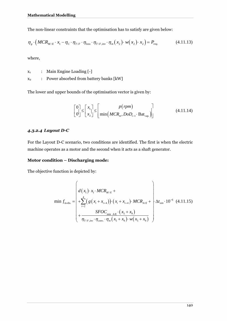
Mathematical Modelling
140
The non-linear constraints that the optimisation has to satisfy are given below:
/ 1 / / , 2 2 2 .g M E C T F loss T F inv m reqMCR x x w x x P (4.11.13)
where,
x1 : Main Engine Loading [-]
x2 : Power absorbed from battery banks [kW]
The lower and upper bounds of the optimisation vector is given by:
1
2 1 cap.
0
0 min , Batm t
p rpmx
x MCR DoD
(4.11.14)
4.3.2.4 Layout D-C
For the Layout D-C scenario, two conditions are identified. The first is when the electric
machine operates as a motor and the second when it acts as a shaft generator.
Motor condition – Discharging mode:
The objective function is depicted by:
1 1 /
46
m-dis. 4 4 /
2
5 9min A/E
/ , . 5 9 5 9
min 10
M E
i i i i A E sim
i
T F inv conv m
d x x MCR
f g x x x x MCR t
SFOC x x
x x w x x
(4.11.15)

Chapter 4
141
The lower and upper bounds of the optimisation vector is given by:
1
2
3
4
cap.5
6
7
8
9cap.
0.61
01
01
0
min , 1 Bat0
0 1
0 1
0 1
0 1 Bat
m in
in
p rpmx
x
x
x
MCR DoDX x
x
x
x
x DoD
(4.11.16)
where,
x1 : Main Engine load [-]
x2 – x4 : Auxiliary load intended for propulsion [-]
x5 : Battery power intended for propulsion [kW]
x6 – x8 : Auxiliary load intended for hotel loads [-]
x9 : Battery power intended for hotel loads [kW]
The linear constraints which are applicable to the D-C motor discharging scenario:
The A matrix:
/ / /
1 0 0 0 0 0 0 0 0
0 1 0 0 0 1 0 0 0
0 0 1 0 0 0 1 0 0
0 0 0 1 0 0 0 1 0
0 0 0 0 1 0 0 0 1
0 1 0 0 0 0A E A E A E
A
MCR MCR MCR
(4.11.17)
and the b vector by:
cap.
1
1
1
1
1 Batin
m
DoD
MCR
b (4.11.18)

Mathematical Modelling
142
The non-linear constraints for the scenario where the electric machine operates as an
electric motor are defined by equations (4.11.19) – (4.11.20).
For the propulsion load demand loads in discharging mode it can be extracted that:
4
1 / / 5 / /
2
/ 5 / , 5 10 5
M E g m A E C T F loss i A E
i
g m A E C loss T F inv shaft
x MCR P x x MCR
P x w x x x P
(4.11.19)
For the auxiliary loads in discharging mode, it can be written that:
9
/ / , 5 10 10 .
6
i A E loss T F inv aux
i
x MCR w x x x P
(4.11.20)
Motor condition – Charging mode:
The objective function is given by:
64charg. 4 / , min
1
min 10n
m i i T F inv sim
i BB bat
xf g x x x w SFOC t
N V
(4.11.21)
The lower and upper bounds of the optimisation vector is given by:
1
2
3
4
cap.cap. 5
0
01
01
01
Batmin Bat , Batinin
sim
p rpmx
x
X x
xE
DoDDoD xt
(4.11.22)
where,
x1 : Main Engine load [-]
x2 – x4 : Auxiliary load [-]
x5 : Battery charged power [kW]
The linear constraints which are applicable to the D-C motor charging scenario:
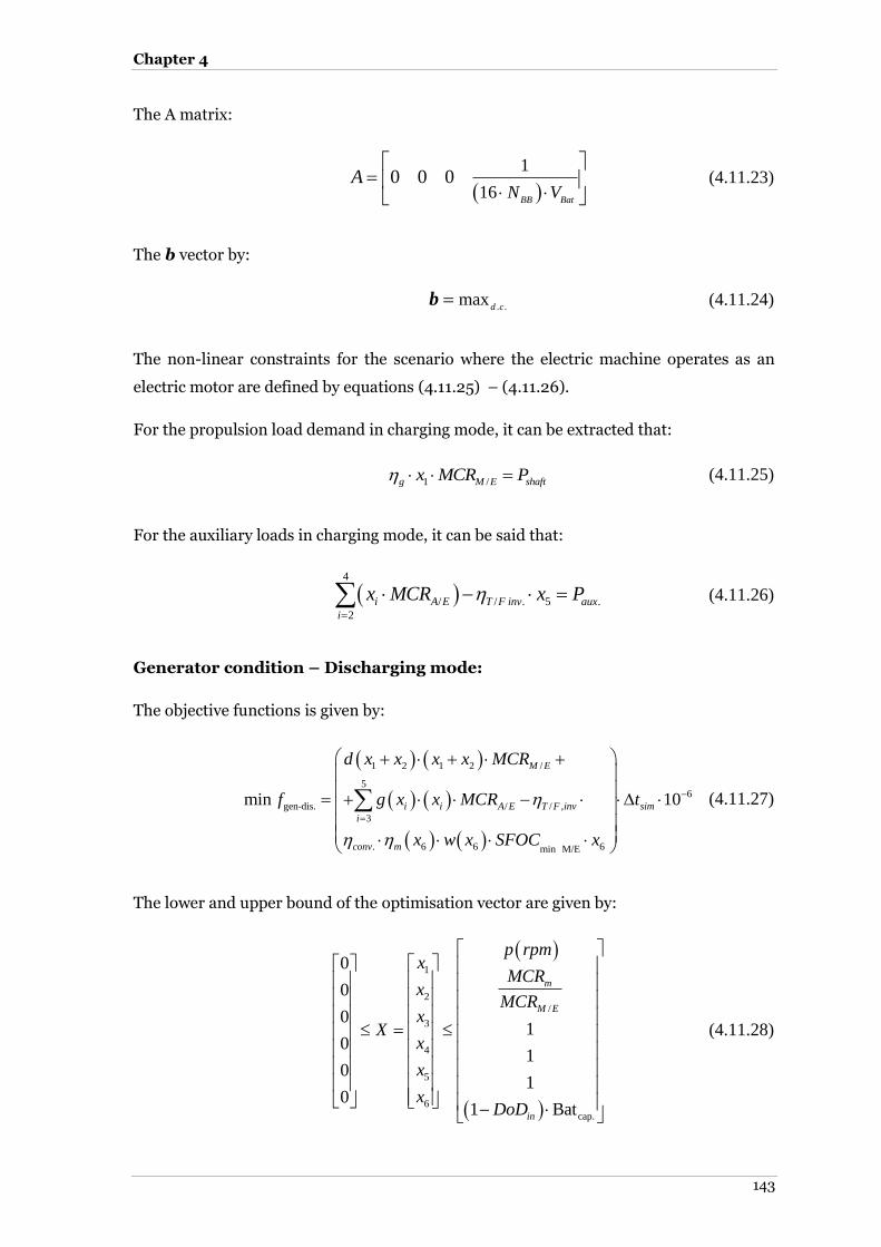
Chapter 4
143
The A matrix:
1
160 0 0
BB BatN V
A
(4.11.23)
The b vector by:
. .
maxd c
b (4.11.24)
The non-linear constraints for the scenario where the electric machine operates as an
electric motor are defined by equations (4.11.25) – (4.11.26).
For the propulsion load demand in charging mode, it can be extracted that:
1 /g M E shaftx MCR P (4.11.25)
For the auxiliary loads in charging mode, it can be said that:
4
/ / . 5 .
2
i A E T F inv aux
i
x MCR x P
(4.11.26)
Generator condition – Discharging mode:
The objective functions is given by:
1 2 1 2 /
56
gen-dis. / / ,
3
. 6 6 6min M/E
min 10
M E
i i A E T F inv sim
i
conv m
d x x x x MCR
f g x x MCR t
x w x SFOC x
(4.11.27)
The lower and upper bound of the optimisation vector are given by:
1
2
/
3
4
5
6
cap.
0
0
01
01
01
01 Bat
m
M E
in
p rpmx
MCRx
MCRx
Xx
x
xDoD
(4.11.28)
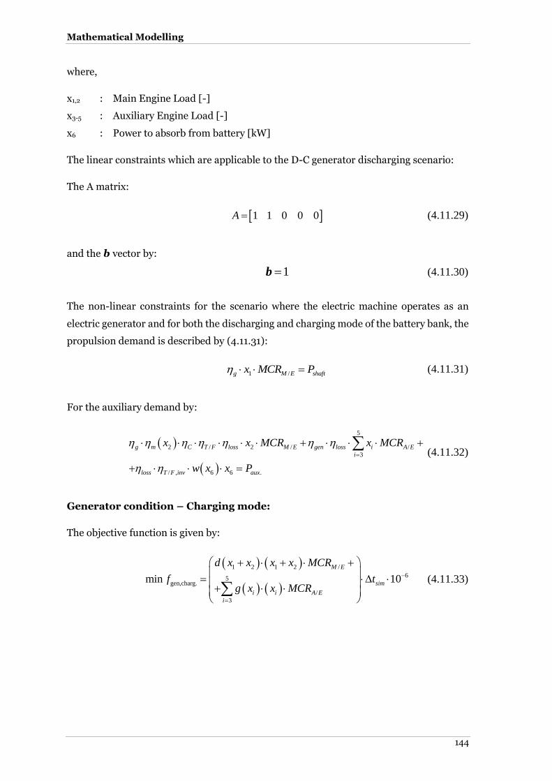
Mathematical Modelling
144
where,
x1,2 : Main Engine Load [-]
x3-5 : Auxiliary Engine Load [-]
x6 : Power to absorb from battery [kW]
The linear constraints which are applicable to the D-C generator discharging scenario:
The A matrix:
1 1 0 0 0A (4.11.29)
and the b vector by:
1b (4.11.30)
The non-linear constraints for the scenario where the electric machine operates as an
electric generator and for both the discharging and charging mode of the battery bank, the
propulsion demand is described by (4.11.31):
1 /g M E shaftx MCR P (4.11.31)
For the auxiliary demand by:
5
2 / 2 / /
3
/ , 6 6 .
g m C T F loss M E gen loss i A E
i
loss T F inv aux
x x MCR x MCR
w x x P
(4.11.32)
Generator condition – Charging mode:
The objective function is given by:
1 2 1 2 /
65
gen,charg.
/
3
min 10
M E
sim
i i A E
i
d x x x x MCR
f tg x x MCR
(4.11.33)

Chapter 4
145
The lower and upper bounds of the optimisation vector are given by:
1
2/
3
4
5
cap. 6
cap.
0 1
0
0
0 1
0 1
1min Bat ,
Bat
m
M E
Batin
insim
xMCR
xMCR
xX
x
xE
DoD xDoDt
(4.11.34)
where,
x1,2 : Main Engine Load [-]
x3-5 : Auxiliary Engine Load [-]
x6 : Power to charge from battery [kW]
The linear constraints which are applicable to the D-C generator charging scenario:
The A matrix:
1 1 0 0 0 0A (4.11.35)
The b vector by:
1b (4.11.36)
The non-linear constraints for this scenario for the auxiliary and charging loads, can be
expressed as follows:
5
2 / 2 / /
3
.
/ ,
1
g m C T F loss M E gen loss i A E
i
Bat
sim Bataux
loss T F inv BB Bat sim
x x MCR x MCR
E
t Ew P
N V t
(4.11.37)
The global minimum is found by comparing charging and discharging in motor mode,
yielding to the local minimum 1. The process is repeated for the generator mode, finding
the local minimum 2. The global minimum is the minimum of the two local minima. Logic
criteria are applied, as mentioned in 4.3.2.1, the difference being that when the system is
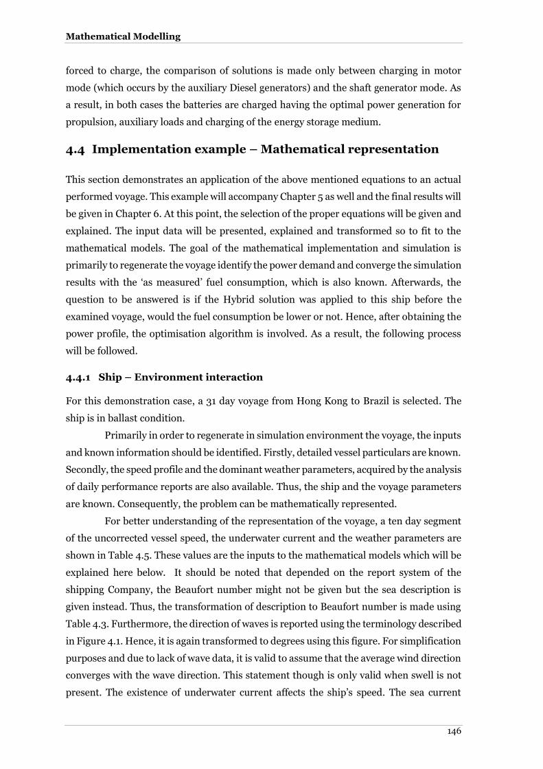
Mathematical Modelling
146
forced to charge, the comparison of solutions is made only between charging in motor
mode (which occurs by the auxiliary Diesel generators) and the shaft generator mode. As
a result, in both cases the batteries are charged having the optimal power generation for
propulsion, auxiliary loads and charging of the energy storage medium.
4.4 Implementation example – Mathematical representation
This section demonstrates an application of the above mentioned equations to an actual
performed voyage. This example will accompany Chapter 5 as well and the final results will
be given in Chapter 6. At this point, the selection of the proper equations will be given and
explained. The input data will be presented, explained and transformed so to fit to the
mathematical models. The goal of the mathematical implementation and simulation is
primarily to regenerate the voyage identify the power demand and converge the simulation
results with the ‘as measured’ fuel consumption, which is also known. Afterwards, the
question to be answered is if the Hybrid solution was applied to this ship before the
examined voyage, would the fuel consumption be lower or not. Hence, after obtaining the
power profile, the optimisation algorithm is involved. As a result, the following process
will be followed.
4.4.1 Ship – Environment interaction
For this demonstration case, a 31 day voyage from Hong Kong to Brazil is selected. The
ship is in ballast condition.
Primarily in order to regenerate in simulation environment the voyage, the inputs
and known information should be identified. Firstly, detailed vessel particulars are known.
Secondly, the speed profile and the dominant weather parameters, acquired by the analysis
of daily performance reports are also available. Thus, the ship and the voyage parameters
are known. Consequently, the problem can be mathematically represented.
For better understanding of the representation of the voyage, a ten day segment
of the uncorrected vessel speed, the underwater current and the weather parameters are
shown in Table 4.5. These values are the inputs to the mathematical models which will be
explained here below. It should be noted that depended on the report system of the
shipping Company, the Beaufort number might not be given but the sea description is
given instead. Thus, the transformation of description to Beaufort number is made using
Table 4.3. Furthermore, the direction of waves is reported using the terminology described
in Figure 4.1. Hence, it is again transformed to degrees using this figure. For simplification
purposes and due to lack of wave data, it is valid to assume that the average wind direction
converges with the wave direction. This statement though is only valid when swell is not
present. The existence of underwater current affects the ship’s speed. The sea current

Chapter 4
147
speed is approximated by the ship’s Master by comparing the speed over ground of the
vessel and the indication on the bridge panel of the speed log/ Doppler. This difference
under normal external conditions gives a good estimation of the underwater current.
Furthermore, in order to reduce the implied error, the values before are transmitted to the
shore office are crosschecked with the sea current charts of the operating area.
Table 4.5: Sample of data interpretation for ship voyage simulation
Time step
Uncorrected vessel speed [knots]
Wind Direction [deg]
Beaufort Number [-]
Underwater current speed [knots]
Corrected vessel speed [knots]
1 14.84 “abeam” =
110 “rough”= 5 “astern”= 0.5 14.34
2 14.46 110 5 0.5 13.96 3 14 0 5 -0.5 14.5 4 14.29 0 6 -0.5 14.79 5 14.92 45 6 0.5 14.42 6 13.63 45 6 -0.5 14.13 7 15.12 135 3 0 15.12 8 14.79 135 5 0.5 14.29 9 14.83 135 6 0.5 14.33 10 14.24 135 6 0.5 13.74
In order to estimate the fuel consumption, the main engine consumption model is
required. According to the mathematical implementation, the engine model demands a
known power profile so to be multiplied by the corrected SFOC and the operational time.
Thus, so that to identify the SFOC of the prime mover, the fuel low calorific value, the
operating temperature should be known. As a result the percentage increase estimated by
equation (4.6.4) can be inserted to the calculations. Nonetheless, the question to be raised
is how to identify the power demand. The connection between the engine and the ship is
established through the use of the propeller model which is mathematically presented in
(4.1.5.1). The best method to implement the propeller is by using the Wageningen B series
approximation which requires though a full set of propeller characteristics, shown in
equation set (4.5.5). Consequently, if the propeller characteristics are known, this
approximation is used. Nevertheless, more information regarding the vessel unique
hydrodynamic parameters is required. For the propeller model the wake friction
coefficient is required. These coefficients and miscellaneous coefficients can be identified
using the material presented in section 4.1.7.
The propeller model in order to give power results requires the ship’s speed and
resistance data. The approximation of resistance is a complex problem and should be
decomposed to calm water resistance, wave resistance, wind resistance, rudder and drift
resistance. Hence, a total set of two (if it is assumed that wave, wind, rudder and drift
resistance are denoted as “added resistance”) resistance components, calm and added

Mathematical Modelling
148
should be identified. The calm water resistance should be identified first. For a given
problem, the question to be answered is why the user should select Holtrop-Mennen
method or Hollenbach approximation. The rule of thumb is to use the model which best
describes the ship resistance if the user has access to the towing tank model tests or to sea
trial measured points. Nonetheless, because in the majority of the applications, this data
is classified or unknown, the following in respect of importance will be assessed so to use
the suitable model:
1. Amount of vessel geometrical information
2. Age of the vessel
3. Hull form
4. Available computational time
Regarding the first parameter, the Holtrop-Mennen method requires a lot of information
which make it unattractive for quick simulation for a given fleet. Nonetheless, it can
describe accurately the majority of designs. However, in unique modern (parameter No 2)
hull forms (parameter No 3), Hollenbach method is suggested. Thus, for the examined
Post-Panamax vessel with dimensions of a regular Panamax ship but with expanded beam
and block coefficient, it is believed from the early beginning that Holtrop-Mennen method
might not describe the problem in laden condition. On the other hand it may better
describe this problem in ballast condition as the hull form in lower drafts yields to typical
hull forms. Thus, by taking into account the above, the calm water resistance will be
approximated by Holtrop method; however, the results should be crosschecked at later
stage with the model data if available.
For this case, the added resistance will be formed by the combination of mean
added resistance models described in 4.1.2.1 – 4.1.2.2 excluding the effect of wind loads
(Kwon, 2008). Aertssen model should be used with caution as it is simple approximation
but yields to modest results. In addition it requires only the length between perpendiculars
of the ship and direction and force of the wind and waves. Kwon model though, uses more
up to date data and applies corrections according to the vessel type, sailing Froude number
and block coefficient. Because the added resistance is a complex problem, the selection of
the model in every case should be done by trial and error method. In case the ship power
demand exceeds regularly the MCR, this means that there is a mismatch of the model and
the reported speed vector or the model is not suitable for this particular simulation case.
For this demonstration case the final selection will be made in Chapter 5 where the
mathematical case will be transformed to Simulink environment.
For the wind resistance, the Blendermann model will be used as it is more up to date
and better describes modern superstructures. Both models in terms of data needs have the

Chapter 4
149
same geometrical information requirements. Thus this parameter does not play any role
to the selection. The rule of thumb for selection the wind resistance is the age of the vessel
and the superstructure type. Usually the age of the ship defines the superstructure form
(examined vessels built in 2005 and onwards).
Concerning the added resistance method of Grigoropoulos (2001), due to the fact
that the vessel coefficients do not drop near the “parent” series forms and also, because
these data do not accurately represent unique designs, this method will not be used.
However, because of the necessary information are known, it will be compared to the rest
mean models in Chapter 5. Although the added resistance models can describe the effect
of wind and waves to the vessel, the lack of sea keeping data inserts a large parameter of
uncertainty. Because RAO information is impossible to be found and detailed towing test
have to be performed, the 4.1.2.3 model will not be used in this thesis. However, in order
to reduce this uncertainty factor, the 4.1.2.4 weather generation coupled with mean models
will be used and demonstrated. This coupling will be analysed in Chapter 5 where the
simulation time step parameters will be discussed.
4.4.2 Coupling power profile and Hybrid system Optimisation
After the mathematical implementation of the ship – environment interaction, the
resistance is transformed to required torque, power and propeller speed. Vessels equipped
with two-stroke Diesel engines have direct propulsion, meaning that no gearbox/ clutch
exits, thus the propeller speed equals to the Diesel engine speed. Therefore, the rotational
speed should remain the same, so that the propeller can maintain the speed of advance
and to produce the required thrust. Furthermore, the production of power, accounting the
transformation losses should be equal to the propeller demand.
For this case, the ECMS strategy will be used as the primary objective is to minimise
the fuel consumption only. Based on the equation set described in 4.3.2, the D-B and D-C
scenarios are applicable to this case. Consequently, before proceeding, the required
information should be identified. Observing the objective functions of D-B power train,
the transformation losses, the engine MCR and the minimum SFOC of the engine are
required. These parameters are static, thus are inserted to the calculations. However, the
battery and the engine fuel efficiencies are load dependent and are not linear. Based on the
Diesel engine fuel efficiency curves of Chapter 3, these curves can be represented by
polynomials of 3rd degree and up, thus the optimisation problem is non-linear. Therefore,
data fitting should be performed and equation for SFOC versus engine load should be
created (g(x) or h(x)). The same is applied to the battery charge and discharge efficiencies
creating the w(x) function.

Mathematical Modelling
150
The case is now mathematically represented. The inputs and outputs are defined.
What remains is how to couple the different time steps and response time for each sub-
model so to form the complete simulation. This will be described in Chapter 5, where the
Simulink representation will be given prior to the continuation of this example.
4.5 Chapter summary
In this chapter, the governing equations for the ship simulator and the optimisation
algorithm were presented. Regarding the ship simulator, a set of models was implemented
for each of the vessel’s calm water resistance. In addition, the propeller and engine models
were also implemented. Furthermore, a mathematical representation of the actual vessel
operation was shown. Concerning the data entry part, environment generation models
were investigated and presented in this chapter. Consequently, a large number of
mathematical models is available for the construction of the simulation blocks. The
description of the simulator blocks will be performed in Chapter 5.
For the Diesel configuration optimisation, two strategies were demonstrated. The
first applied the ECMS strategy for fuel oil consumption reduction. The second algorithm,
named as ‘pseudo multi-objective’ targeted primarily the fuel consumption when the
system is discharging and secondly at the reduction of PM while the system was charging.
The results of the ECMS strategy for Diesel Hybrid power trains are presented in
Chapter 6.

Chapter 5
151
5 Ship Voyage Simulator
Townsin et al. (1975) underlined the importance of monitoring the speed performance of
ships. Two main reasons for monitoring the ship performance are charter party conditions
and studying bad weather performance. For that reason, it is of vital importance to
demonstrate a non-complex, reality-based simulation tool for the ship voyage.
The identification of patterns or of operational randomness will facilitate the
construction of valid test cases and simulation scenarios. The latter will assess primarily
the feasibility of the mathematical modelling and, secondly, the propulsion machinery
optimisation outputs in artificial conditions, based, however, on reality scenarios.
Therefore, the proposed simulation tool accounts for the mathematical implementation of
ship and propulsion components and of charter party agreement requirements. As a result,
based on the management profiles of a large number of shipping companies, the operation
of the vessel is defined by the charter type. In the event of operation in the spot market,
the vessel increases its speed in order to reduce the time spent in the leg, so as to arrive
early at the discharge port and probably receive a demurrage. Alternatively, it is observed
that during years of economic growth when demand is high, shipping companies decide to
break the charter party agreement of unloading the goods at a predefined time and unload
the cargo earlier by paying a penalty, in order to catch the next freight that is far more
profitable for the ship-owner. In this case, the vessel regularly operates at a predefined and
high speed without accounting for the increase in power requirement (Lorange, 2005).
This approach can be characterised as constant speed. When the vessel operates in time
charter, only the distance is predefined and the master usually defines the vessel speed in
order to arrive during the predefined time slot at the arrival port based on a three day or
seven day weather forecast. Usually, the setting is for ‘constant RPM’ during each day, and
re-adjusted accordingly if the ETA is revised. The final operation scenario that was
investigated was the predefined distance to be covered during the voyage day. Actually,
this scenario is a mixture of constant power and constant speed during the examined
increment and relies on the master’s decisions. In the simulation environment, a pseudo
decision making process was inserted using two simple principles. The first principle was
to set a power limit versus sea state, which is usually defined by safety standards for
voluntary speed reduction due to slamming, heavy vertical accelerations forward and
racing of the propeller (Journee and Meijers, 1980), and by the operations department of
the maritime corporation. The second principle is to implement a negative coefficient that
accounts for the ‘off-target percentage’, which is dependent on the elapsed time and the
miles to go. A simple logical operator was inserted to switch from the constant power
setting to constant speed, in order to cover the desired daily distance. It is obvious that the

Ship Voyage Simulator
152
vessel speed is altered significantly when the elapsed time reaches 24 hours, and still the
off target percentage is not equal to zero, indicating that this is not an optimised solution
as decision modelling was not attempted in this project.
5.1 Simulation implementation
This section presents the implementation of the mathematical equations with a graphical
programming representation using the Simulink environment. The Simulink environment
is offered together with the Matlab® Suite, developed by Mathworks 6 . Simulink is a
software package for modelling, simulating, and analysing dynamic systems. It supports
linear and nonlinear systems, modelled in continuous time, sampled time, or a hybrid of
the two. Systems can also be multi-rate, i.e. have different parts that are sampled or
updated at different rates. For modelling, Simulink provides a graphical user interface
(GUI) for building models as block diagrams. With this interface, the models are drawn
easily, with ‘drag and drop’, in contrast to conventional simulation packages that formulate
differential equations and difference equations in a compiled language or program.
Moreover, a predefined template function to write the code of the mathematical
implementation is used. This template is called S-function and significantly reduces the
code complexity (Mathworks, 2002).
The simulation blocks consist of logical separation of the mathematical models;
for example, one simulation block represents the calm water resistance and a different the
wind induced loads. With the modular, scalable and extendable technique, the simulation
tool can be further improved by replacing the models with more complex ones, and can be
updated if there are changes in the governing equations, i.e. to include modern hull forms
similar to the updates proposed by Kwon (2008) for the mean added resistance
approximation.
The input and the output of each sub-model are achieved by the block connection
ports. For each block, the number of inputs and outputs is defined, thus appropriate
connection points are made in order to interconnect with the remaining simulator blocks.
In the Simulink environment, the connection of the blocks is represented using
signal arrows. These arrows can be grouped together into a single bus either they can be
connected to a signal transmitter block. Both ways aim to reduce the graphical complexity
of the simulation representation.
In order to avoid a complex diagram for the entire fleet, it is proposed to group
similar blocks and form major blocks (e.g. fleet calm resistance major block). The approach
using signal buses and major blocks significantly reduces the programming error.
6 Matlab® version 2011b, www.mathworks.com
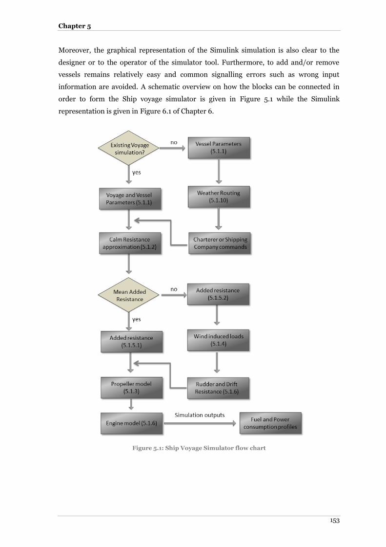
Chapter 5
153
Moreover, the graphical representation of the Simulink simulation is also clear to the
designer or to the operator of the simulator tool. Furthermore, to add and/or remove
vessels remains relatively easy and common signalling errors such as wrong input
information are avoided. A schematic overview on how the blocks can be connected in
order to form the Ship voyage simulator is given in Figure 5.1 while the Simulink
representation is given in Figure 6.1 of Chapter 6.
Figure 5.1: Ship Voyage Simulator flow chart
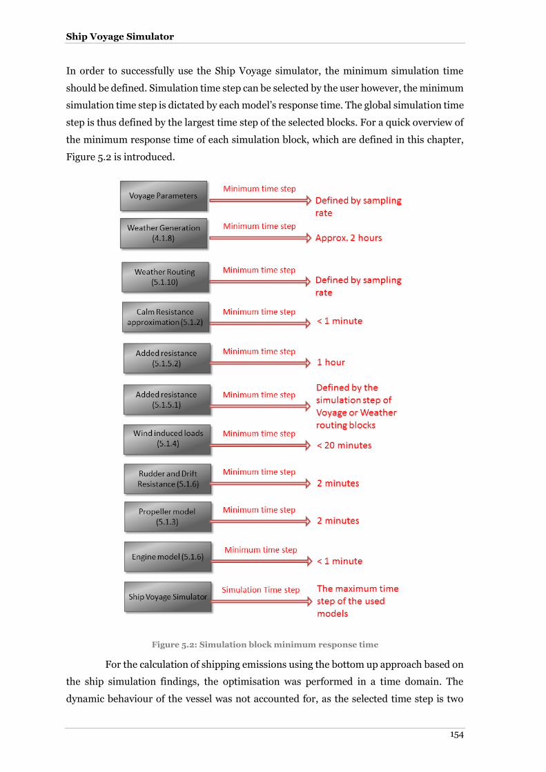
Ship Voyage Simulator
154
In order to successfully use the Ship Voyage simulator, the minimum simulation time
should be defined. Simulation time step can be selected by the user however, the minimum
simulation time step is dictated by each model’s response time. The global simulation time
step is thus defined by the largest time step of the selected blocks. For a quick overview of
the minimum response time of each simulation block, which are defined in this chapter,
Figure 5.2 is introduced.
Figure 5.2: Simulation block minimum response time
For the calculation of shipping emissions using the bottom up approach based on
the ship simulation findings, the optimisation was performed in a time domain. The
dynamic behaviour of the vessel was not accounted for, as the selected time step is two

Chapter 5
155
hours. This can be justified by the fact that emissions are quasi-static phenomena and the
transient operation of the machinery does not need to be simulated. During transient
phenomena, the emission calculation using fuel based or power based factors does not
represent the actual emission phenomena and, in addition, no modelling of emissions
during the dynamic phenomenon is accurate to this date. Thus, the dynamic approach is
rejected, and a time step more than five minutes is required, as a result. However, the
absence of the response amplitude operator (RAO) of added resistance in induced wind
and waves (which requires detailed model basin tests and or runs of complex sea keeping
codes) given a specific sea state (significant wave height and modal period) has led to the
adoption of a two hour simulation time step, with the reasons for this adoption having
been discussed in Chapter 4. The simulation models follow the SI unit system. When other
units are required in interpolation tables, appropriate conversion is performed at a local
stage.
5.1.1 Input data blocks
The simulations require a set of inputs in order to perform the necessary calculations and
produce their outputs, which then can be used as inputs to other blocks. The basis of this
process is made at the input data blocks. Their implementation is simplistic, as the
variables are fed by input values by the user in a text data form. Each variable name is
unique in the data form and has exactly the same name in the Simulink environment.
Consequently, the values are fed to the appropriate output ports and the information can
then pass to the other blocks. With this approach, the blocks are not changed within the
Simulink program, but the user can modify the input file, which then re-assigns the values
to the appropriate variables. Two blocks of this type are found in the developed simulator
package. The first block, coloured in blue, contains the hydrodynamic and geometrical data
for the examined vessel and is identified as ‘ship particulars block’. The second block,
denoted in dark yellow, contains the propeller characteristics and information regarding
the bulbous bow and is referred as ‘propeller data block’. The block coloured in white
contains information regarding air and sea environmental conditions, such as
temperatures, but not the wind velocity or the Beaufort number, which are produced by
the signal generator block. The latter is fed by values produced by the process of random
weather generation defined in chapter 4. Nevertheless, if the simulation is about an actual
voyage, the master’s reported data included in the ‘noon report’ are inserted, along with
the reported vessel speed. This process simplifies the simulation procedure as the data is
not manually transformed into the Simulink but at the input stage. Using that topology,
the simulation can be performed at a very short time for the complete fleet if data is
available, producing a global solution.
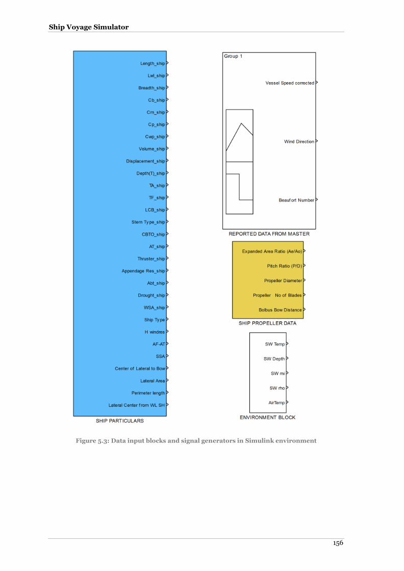
Ship Voyage Simulator
156
Figure 5.3: Data input blocks and signal generators in Simulink environment

Chapter 5
157
5.1.2 Calm water resistance block
The simulation blocks describe the equation set of subchapter (4.1.1) for both resistance
approximation methods. In addition the wake, thrust deduction and relative rotative
coefficients are defined by the equation set of subchapter (4.1.7).
5.1.2.1 The Holtrop-Mennen calm water approximation method
For the approximation of calm water resistance using the aforementioned method, a large
number of geometrical vessel data is required. Due to the requirement of a detailed
geometry of the ship, where – in the case of a globalisation of the simulator – such
information may not be available, this method should be avoided. However, the existence
of this block is necessary as it is where hydrodynamic coefficients required by the propeller
and engine blocks are calculated.
The Holtrop Mennen resistance block is connected to the ‘ship particulars block’,
the ‘propeller data block’, which are considered as input blocks. Their definition is
described later in subchapter 5.2.9. The outputs of this block, with the exception of the
calm resistance, are connected to the propeller block, whether it is the B-Series
approximation or the actual propeller characteristics block.
Table 5.1: Holtrop Mennen resistance block inputs and outputs
Model Inputs Model Outputs Lwl, B, D, lcb, CB, CM, CP, CWP, fore and aft Draft,
mean Draft, Drought, Displacement volume Wetted Surface Area, Immersed transom area,
Thruster diameter, Stern type, Bolbus bow cross sectional area, Bow thruster added
resistance
Calm Water Resistance
Appendage Resistance (Holtrop look up table) Wake coefficient Vessel’s speed Thrust deduction coefficient
Sea water kinematic viscosity Relative rotation coefficient Sea water density
Sea water depth
Expanded Blade Area ratio Pitch to Diameter ratio
It can be seen in the block description of Figure 5.4 that the simulator user can switch
between the approximations of the hydrodynamic coefficients with Holtrop-Mennen and
other methods, as found in subchapter 4.1.7.
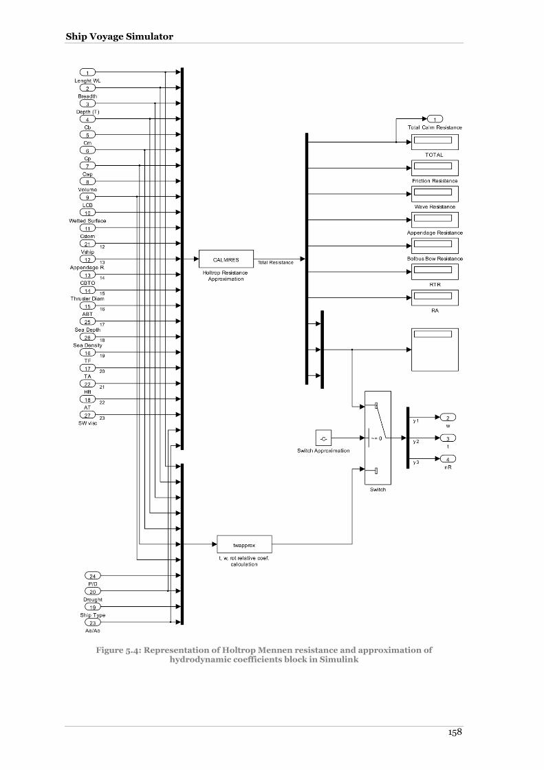
Ship Voyage Simulator
158
Figure 5.4: Representation of Holtrop Mennen resistance and approximation of hydrodynamic coefficients block in Simulink

Chapter 5
159
5.1.2.2 The Hollenbach calm water approximation method
The Hollenbach method requires a smaller set of data compared to the Holtrop Mennen
method. This block has no wake, thrust or rotative efficiency coefficient approximation,
thus it is proposed to be used in combination with the Holtrop Mennen block. Moreover,
it is recommended that the resistance approximation results of the two methods be
compared to each other, in order to identify the method that converges in a better way with
the actual ship resistance.
Figure 5.5: Representation of the Hollenbach resistance block in Simulink
The Hollenbach method approximates the residual resistance only. For the friction
resistance, the method of ITTC is adopted but for a wetted surface area approximated by

Ship Voyage Simulator
160
the method. The friction resistance is the third output of the S-function block and the result
can be checked on the screen by the display sink block.
Table 5.2: Hollenbach resistance block inputs and outputs
Model Inputs Model Outputs Lwl, LBP, Los, B, CB, fore and aft Draft, Number
of Bosses, Number of bilges, Number of Rudders
Calm Water Resistance Vessel’s speed
Sea water kinematic viscosity Sea water density
For simplicity purposes, the S-function block through the first port exports the total
resistance, which is the sum of the friction resistance (port 3) and the residual resistance
(port 2). Due to its application in bulk carriers, this particular model has as constants the
number of bilges (one propeller vessels), the number of propeller boss and the number of
bow thrusters, which is set to zero as the sampled vessels are not equipped with bow
thrusters. The propeller shaft is not supported by brackets thus the number is set to zero.
5.1.3 Propeller block
This block is responsible for matching the resistance with the production of thrust, given
the hydrodynamic coefficients obtained from the resistance blocks. The required
information for the propeller characteristics is imported from the propeller data block. The
output of the system is the propeller developed thrust, the propeller torque and the
rotational speed. Finally, the required engine power to propel the vessel is estimated, given
the speed request.
Table 5.3: Propeller block inputs and outputs
Model Inputs Model Outputs Expanded Blade Area ratio Propeller Thrust
Pitch to Diameter ratio Propeller Torque Number of propeller blades Propeller RPM
Wake coefficient Required Engine power Thrust deduction coefficient
Relative rotation coefficient Sea water kinematic viscosity
Sea water density Propeller shaft efficiency Vessel’s total resistance
Vessel’s speed
It can be seen from the schematic of the Simulink model that the user can easily switch
between the actual propeller data and the B-series approximation. However, the existence
of the two models increases the computer power demand, thus the simulation time. In
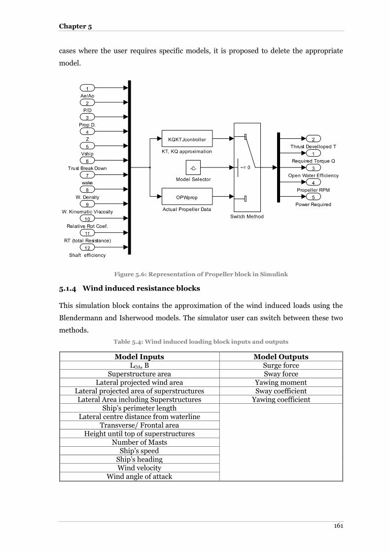
Chapter 5
161
cases where the user requires specific models, it is proposed to delete the appropriate
model.
Figure 5.6: Representation of Propeller block in Simulink
5.1.4 Wind induced resistance blocks
This simulation block contains the approximation of the wind induced loads using the
Blendermann and Isherwood models. The simulator user can switch between these two
methods.
Table 5.4: Wind induced loading block inputs and outputs
Model Inputs Model Outputs LOA, B Surge force
Superstructure area Sway force Lateral projected wind area Yawing moment
Lateral projected area of superstructures Sway coefficient Lateral Area including Superstructures Yawing coefficient
Ship’s perimeter length
Lateral centre distance from waterline Transverse/ Frontal area
Height until top of superstructures Number of Masts
Ship’s speed Ship’s heading Wind velocity
Wind angle of attack
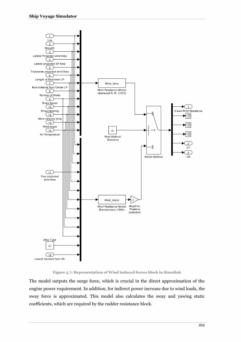
Ship Voyage Simulator
162
Figure 5.7: Representation of Wind induced forces block in Simulink
The model outputs the surge force, which is crucial in the direct approximation of the
engine power requirement. In addition, for indirect power increase due to wind loads, the
sway force is approximated. This model also calculates the sway and yawing static
coefficients, which are required by the rudder resistance block.

Chapter 5
163
This model necessitates the knowledge of various geometrical characteristics of
the vessel. This information regards the area above the water line because that part of the
construction is exposed to the wind. The resistance components are added together into a
resistance sink in order to form the total ship resistance given the specific vessel speed and
the dominating environmental parameters.
5.1.5 Added resistance blocks
For the approximation of added resistance, two approximation methods are proposed. For
a more complex method, but with introduced uncertainty, the Series 60 added resistance
with the use of interpolation tables is modelled.
5.1.5.1 The Aertssen and Kwon block
The Aertssen and Kwon methods rely on the knowledge of simple vessel characteristics
and the Froude number. In addition, the simple wind wave characteristics, such as the
angle of attack and the force expressed in Beaufort number, are required. This block uses
an interpolation table to estimate the minimum and maximum occurrence value of wind
speed given the sea state. When these two values have been identified, a random number
generator produces a wind value into the range defined by the interpolation matrix.
Figure 5.8: Representation of Added resistance block in Simulink

Ship Voyage Simulator
164
Table 5.5: Aetrssen and Kwon block inputs and outputs
Model Inputs Model Outputs
LOA, CB, Displacement volume Surge force percentage of calm
resistance Beaufort Number
Ship type (interpolation table for Blendermann
model) Wave angle of Attack
Ship’s speed
5.1.5.2 Series 60 added resistance block
This block uses a set of matrices to approximate the non-dimensional added resistance
value for an equivalent vessel of the series 60 models of the same L/B and B/T ratio and
CB. In order to estimate the actual value of added resistance, the vessel characteristics, the
wind direction and the significant wave height are inserted into the calculation and the
final value of added resistance is given in algebraic form. This procedure is implemented
using four-dimension interpolation data. Firstly, based on the Grigoropoulos et al. (2001)
publication, the tabular data for added resistance for two B/T ratios have been utilised.
The acquired set of data is for the given vessel CB and for L/B ratio as close as to the ratio
of the examined vessel. In the event that there is a notable difference between the vessel
L/B ratio and the Series 60 model, the recommended procedure is to perform
interpolation between L/B and then B/T. Due to the fact that a five-dimension
interpolation matrix does not exist in Simulink environment, this approximation
technique will require two four-dimension lookup tables and then a two-dimension lookup
table for the final interpolation for the examined L/B and B/T. The four-dimension matrix
requires information regarding the wave peak modal period (port 1), the wave direction
(port 2), the vessel sailing Froude number (port 3) and the B/T ratio (port 4).
There are cases that the modal period calculated by the environmental block
outputs values that exceed the interpolation range. During the test cases it was observed
that the modal period is lower than the lower range bound. Thus, a decision switch was
added to the block in order to acquire the minimum interpolation value instead of the
actual. Although it may argued that this adoption introduces errors into the calculations
and for that reason the non-dimensional form of modal period was implemented, this
assumption led to meaningful results because the insertion of lower range value outcomes
strange modal periods that have no physical meaning. The final value is transformed to kN
and then summed to the resistance sink through the block output port one.

Chapter 5
165
Japanese shipyards were the first to identify the importance of model runs in order to
define at an early design stage the appropriate engine sea margin. However, this method,
compared with the actual voyage, introduces uncertainty into the calculations.
Table 5.6: Series 60 added resistance approximation block inputs and outputs
Model Inputs Model Outputs Length between perpendiculars Surge force
Breadth to Draft ratio
Significant wave Height Wave modal period
Wave angle of Attack Ship’s speed
Sea water density Acceleration of gravity
Figure 5.9: Representation of Series 60 added resistance block in Simulink
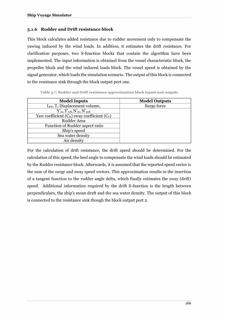
Ship Voyage Simulator
166
5.1.6 Rudder and Drift resistance block
This block calculates added resistance due to rudder movement only to compensate the
yawing induced by the wind loads. In addition, it estimates the drift resistance. For
clarification purposes, two S-function blocks that contain the algorithm have been
implemented. The input information is obtained from the vessel characteristic block, the
propeller block and the wind induced loads block. The vessel speed is obtained by the
signal generator, which loads the simulation scenario. The output of this block is connected
to the resistance sink through the block output port one.
Table 5.7: Rudder and Drift resistance approximation block inputs and outputs
Model Inputs Model Outputs LPP, T, Displacement volume, Surge force
Y’uν, Y’ccδ, N’uν, N’uuδ
Yaw coefficient (CN) sway coefficient (CY) Rudder Area
Function of Rudder aspect ratio Ship’s speed
Sea water density Air density
For the calculation of drift resistance, the drift speed should be determined. For the
calculation of this speed, the heel angle to compensate the wind loads should be estimated
by the Rudder resistance block. Afterwards, it is assumed that the reported speed vector is
the sum of the surge and sway speed vectors. This approximation results in the insertion
of a tangent function to the rudder angle delta, which finally estimates the sway (drift)
speed. Additional information required by the drift S-function is the length between
perpendiculars, the ship’s mean draft and the sea water density. The output of this block
is connected to the resistance sink though the block output port 2.
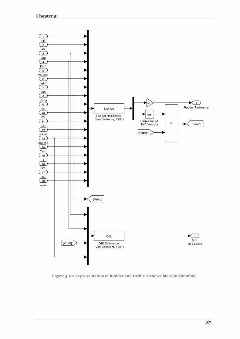
Chapter 5
167
Figure 5.10: Representation of Rudder and Drift resistance block in Simulink
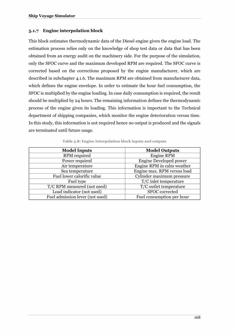
Ship Voyage Simulator
168
5.1.7 Engine interpolation block
This block estimates thermodynamic data of the Diesel engine given the engine load. The
estimation process relies only on the knowledge of shop test data or data that has been
obtained from an energy audit on the machinery side. For the purpose of the simulation,
only the SFOC curve and the maximum developed RPM are required. The SFOC curve is
corrected based on the corrections proposed by the engine manufacturer, which are
described in subchapter 4.1.6. The maximum RPM are obtained from manufacturer data,
which defines the engine envelope. In order to estimate the hour fuel consumption, the
SFOC is multiplied by the engine loading. In case daily consumption is required, the result
should be multiplied by 24 hours. The remaining information defines the thermodynamic
process of the engine given its loading. This information is important to the Technical
department of shipping companies, which monitor the engine deterioration versus time.
In this study, this information is not required hence no output is produced and the signals
are terminated until future usage.
Table 5.8: Engine Interpolation block inputs and outputs
Model Inputs Model Outputs RPM required Engine RPM
Power required Engine Developed power Air temperature Engine RPM in calm weather Sea temperature Engine max. RPM versus load
Fuel lower calorific value Cylinder maximum pressure Fuel type T/C inlet temperature
T/C RPM measured (not used) T/C outlet temperature Load indicator (not used) SFOC corrected
Fuel admission lever (not used) Fuel consumption per hour

Chapter 5
169
Figure 5.11: Representation of Engine interpolation block in Simulink

Ship Voyage Simulator
170
5.1.8 Kinetic Battery Model block
The Kinetic Battery Model is a dynamic simulation model of the battery discharging and
charging. Based on the mathematical equations described in subchapter (4.2.2.2), there is
an exchange of energy between the two wells (Manwell and McGowan, 1993). Due to the
fact that the discharge and charge phenomena are dynamic, differential equations have to
be solved. This block solves the two differential equations and supplies the derivative
though a memory function, in order to proceed with the calculation of the other
parameters, which is the final energy to be absorbed from each well. Nonetheless, the
existence of the memory blocks significantly slows down the simulation process. For that
reason, it is proposed to use the embedded differential equation solver into the S-function
block in order to speed up the process. It has to be noted that in both cases the result should
be the same. In order to increase the block complexity, a two-dimension lookup table is
implemented that describes the cell/battery voltage drop versus the current. In case that
the simulation implies extra accuracy, the lookup table output shall replace the fourth
input port. The SoC and the discharge/charge current can be further calculated by the
existing block outputs.
Figure 5.12: Representation of KiBaM battery block in Simulink
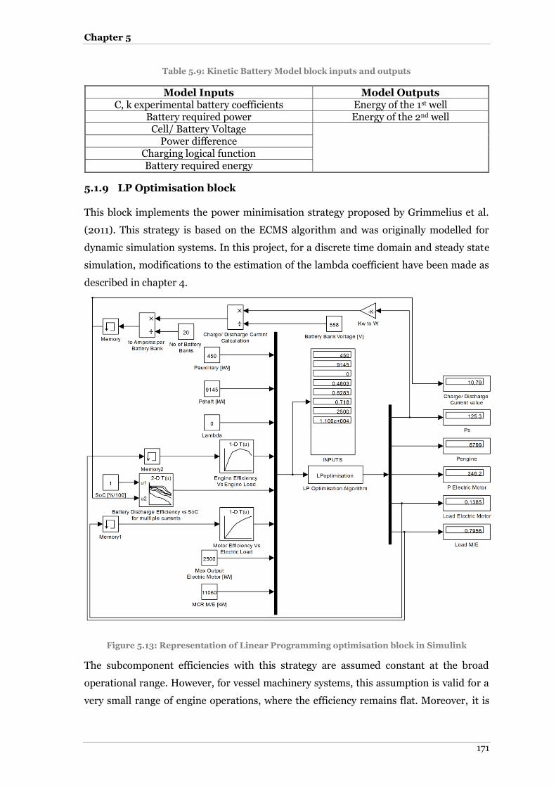
Chapter 5
171
Table 5.9: Kinetic Battery Model block inputs and outputs
Model Inputs Model Outputs C, k experimental battery coefficients Energy of the 1st well
Battery required power Energy of the 2nd well Cell/ Battery Voltage
Power difference
Charging logical function Battery required energy
5.1.9 LP Optimisation block
This block implements the power minimisation strategy proposed by Grimmelius et al.
(2011). This strategy is based on the ECMS algorithm and was originally modelled for
dynamic simulation systems. In this project, for a discrete time domain and steady state
simulation, modifications to the estimation of the lambda coefficient have been made as
described in chapter 4.
Figure 5.13: Representation of Linear Programming optimisation block in Simulink
The subcomponent efficiencies with this strategy are assumed constant at the broad
operational range. However, for vessel machinery systems, this assumption is valid for a
very small range of engine operations, where the efficiency remains flat. Moreover, it is

Ship Voyage Simulator
172
valid for battery systems that operate under constant current for a time period where the
voltage drop is constant.
This block incorporates the Hybrid component efficiencies in the form of a lookup
table. The engine efficiency, the electric motor efficiency is a one-dimension lookup table
with engine or motor load as the interpolating vector. For the battery efficiency, the lookup
table is more complex, as the battery discharge efficiency depends on the State of Charge,
which is the first input, as can be seen in Figure 5.13, and the discharge current as the
second input. Given the fact the LP S-function block yields to the loads of electric machine
and M/E, which feed the input of the efficiency lookup tables, multiple algebraic loops are
present. In order to solve this problem, memory blocks have been inserted to the model,
which are responsible for supplying the previous simulation step values, enabling the
system to run. Nonetheless, the simulation time is increased significantly and for large
variations where the efficiencies are not constant, the outputs are not valid, thus it is
suggested to run the optimisation script described in Chapter 4.
Table 5.10: LP optimisation block inputs and outputs
Model Inputs Model Outputs Number of battery banks (NBB) Battery storage power exchange
Auxiliary required Power M/E power output Propulsive required Power Electric machine power output
λ coefficient Electric machine load Battery SoC M/E load
Electric machine MCR
M/E MCR
5.1.10 Weather routing capability
The ship simulator can be also used for weather routing decisions as it is a non- complex
fast package. The importance of routing for reduction of fuel consumption, voyage time
and increased passage safety was established in the early years of ocean going shipping. In
order to decrease the consumption of power due to added and wind resistance, it was
necessary to identify ways to optimise the route. The first attempt, however, was made by
James (1957), and Hanssen and James (1960). In their study, the use of an isochrones
time-front method based on weather forecast data, which attempted to minimise the
journey time, was demonstrated. James’ (1957) method was based on empirical results
studying the effect of the waves while the ship proceeds into them at different speeds.
Haltiner et al. (1962) published a new approach with the use of calculus variations. This
method was used later by Papadakis et al. (1989), who described the ship speed as a
function of the significant wave height and direction. Zoppoli (1974) produced the first
dynamic approach for optimisation of routing based on James’ (1957) results, by setting
wave height and direction as random parameters. Work on minimisation of voyage time is

Chapter 5
173
performed by Bijlsma (1975) as well, who proposed alternative solutions for fuel savings
and routing optimisation. Frankel and Chen (1978) used the Bretschneider wave spectrum
to match sea state conditions with random wave frequency, direction and height. It was
the first time that the problem was not approached with empirical curve methods, and a
physics implementation was followed to simulate the wave energy and direction. Lo and
McCord (1998) used global data for ocean currents with the addition of data
measurements from ship voyage weather monitoring, in order to estimate state transition
probabilities. Azaron and Kianfar (2003) used the directed acyclic network theory to find
the shortest route. The goal was to decide for each geographical position of the vessel
whether it would be optimum to change its position and towards which direction. Vlachos
(2004) attempted to find the optimum solution for a weighted equation of voyage travel
time and safety. To perform the optimisation he followed two separate methods: the use
of an iterative optimisation algorithm, and the simulated annealing method. Speed loss in
waves was described using James’s results. The study was revised in 2008 and 2009 by
the addition of actual experimental data. Hinnenthal and Saetra (2005) used Pareto fronts,
two objective optimization algorithms, and population generation algorithms to create
different routes to minimise simultaneously travel time and fuel consumption. The swell
forecasts used were modelled using the Bretscheider spectrum. Padhy et al. (2007)
employed optimal control theory and a dynamic programming technique to obtain a
reliable optimum route in a given random sea-state. Szłapczyńska and Śmierzchalski
(2008) attempted in their research to use the Isochrones method with area partitioning,
combined with a weather routing system with an evolutionary approach to find alternative
routes of reduced collision risk and low passage cost.
5.2 Simulink block and optimisation algorithm test cases
This section presents the accuracy of the Simulink models given known inputs and
outputs. The algorithm’s outputs were compared with by hand calculation for the specified
given inputs or by comparing the simulation results with published results presented by
the original authors. The Simulink representation of 5.2.1, 5.2.2 comparison is depicted in
Figure 5.18.
5.2.1 Calm water resistance block test
The selection of the calm water resistance model was made by comparing the different
approximation methods presented in Table 4.1. The selected method should best suit the
experimental resistance curve which was obtained from the MOERI (KRISO) model test
basin in Korea. Due to applicability constraints and due to the publication date, five
resistance approximation methods have been compared. It can be observed from Figure
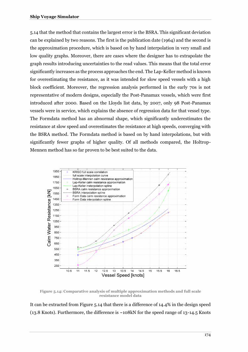
Ship Voyage Simulator
174
5.14 that the method that contains the largest error is the BSRA. This significant deviation
can be explained by two reasons. The first is the publication date (1964) and the second is
the approximation procedure, which is based on by hand interpolation in very small and
low quality graphs. Moreover, there are cases where the designer has to extrapolate the
graph results introducing uncertainties to the read values. This means that the total error
significantly increases as the process approaches the end. The Lap-Keller method is known
for overestimating the resistance, as it was intended for slow speed vessels with a high
block coefficient. Moreover, the regression analysis performed in the early 70s is not
representative of modern designs, especially the Post-Panamax vessels, which were first
introduced after 2000. Based on the Lloyds list data, by 2007, only 98 Post-Panamax
vessels were in service, which explains the absence of regression data for that vessel type.
The Formdata method has an abnormal shape, which significantly underestimates the
resistance at slow speed and overestimates the resistance at high speeds, converging with
the BSRA method. The Formdata method is based on by hand interpolations, but with
significantly fewer graphs of higher quality. Of all methods compared, the Holtrop-
Mennen method has so far proven to be best suited to the data.
Figure 5.14: Comparative analysis of multiple approximation methods and full scale resistance model data
It can be extracted from Figure 5.14 that there is a difference of 14.4% in the design speed
(13.8 Knots). Furthermore, the difference is ~108kN for the speed range of 13-14.5 Knots

Chapter 5
175
and the prediction method follows a cubic trend, as expected. For higher speeds, when
wave-breaking resistance takes place, the error decreases. The approximation curve,
however, has a normal shape for the examined speed range. The last comparison will be
made between the Holtrop-Mennen method and the Hollenbach method. For this purpose,
Figure 5.15 is introduced. The values are corrected for air-drag, which is given for the
examined speed range, and the hull roughness is neglected as the ship is on sea trials.
Based on Figure 5.15, the Hollenbach method slightly overestimates the resistance from
12.5 to 14.3 knots. There is very good matching at 11-12.5 and 14.5 knots, while for high
speeds of >15knots, the method underestimates the total resistance. However, the
introduced error at high speed does not affect the calculations, as the vessel design speed
is 13.81 knots with a maximum reported speed of 14.7 knots in both laden and ballast
conditions.
Differences between this prediction method and the experimental data are due to
the hull design, which has a high block coefficient and small dimensions compared to the
statistical data that the method was based on. Due to the small error introduced, this
method will be considered as best suited for the simulator purpose.
Figure 5.15: Comparative analysis of resistance approximation and model test results for design draft and speed range of 11 – 16 knots

Ship Voyage Simulator
176
5.2.2 Propeller block test
The second comparison will be performed for the purpose of estimating the deviation of
the Wageningen B-series approximation and the actual propeller data as supplied by the
KRISO model basin facility, which performed the propeller tests. The comparison was
performed for ten simulation segments, which correspond to a progressive speed increase
from 11 to 16 knots. It can be observed from the detail of Figure 5.16 that there is
approximately 2.3% difference in the propeller open water efficiency. Nonetheless, the B-
series approximation yields to a very good approach to the actual data and is considered
as an acceptable method in cases where the real propeller performance characteristics are
not available. In order to better understand the effect of this error, the engine propeller
interaction should be evaluated. Two set of tests that couple the resistance model and the
propeller performance have been completed.
Figure 5.17 presents the propeller engine interaction for two thrust resistance
matches. The top figure correlates the thrust resistance match for model test resistance
data.
Figure 5.16: Comparative analysis of B-series approximation and actual propeller data
The curve depicted in diamond symbols represents the engine power and RPM demand to
match the ship’s calm resistance at the design draft, in calm sea, with clean hull and for a

Chapter 5
177
speed range of 11 to 16 knots with the developed thrust. It can be observed that the
propeller efficiency greatly affects the power consumption, thus the propeller is heavily
loaded. In addition, the RPM demand is lower than the actual propeller. However, the
engine propeller matching is not acceptable, since, with the existence of sea margin and
hull foulness, the vessel is unable to absorb the full power of the engine at the maximum
speed. The second figure depicts the engine propeller interaction for thrust resistance
match. The resistance is approximated by the Holtrop-Mennen method. The purpose of
this comparison is to identify the effect of the resistance curve on the engine power and to
conclude which imposed error has greater effect on the total simulation. It can be observed
from Figure 5.17 (lower subplot) that the B-series approximation, in combination with the
Holtrop-Mennen resistance method, leads to a unacceptable propeller engine match. The
propeller cannot absorb the maximum power of the engine, although it does not reach the
speed limit. Nonetheless, the matching of the actual propeller with the Holtrop-Mennen
method leads to an acceptable matching, although the maximum speed is not reached. The
latter is not caused by the simulation block, but by the improper initial design of the vessel.
Figure 5.17: Propeller engine interaction for 2 resistance methods and for B-series approximation compared to actual propeller performance data

Ship Voyage Simulator
178
Thus, the resistance method has a slight effect on the power requirement, but it alters the
propeller rotational speed by approximately 3-5 RPM. By examining Figure 5.17, it can be
concluded that the effect of the resistance on the propeller engine interaction is negligible,
but the approximation of the propeller characteristics greatly affect the simulator
accuracy. This finding necessitates the insertion of the actual propeller data into the ship
voyage simulator, in order to reduce the multiplication of error.

Chapter 5
179
Figure 5.18: Simulink representation for Calm water resistance, propeller and propeller-engine interaction comparative analysis
Input Blocks
Calm Resistance
Block
Model Data for
Propeller Block
Propeller approximation Block

Ship Voyage Simulator
180
5.2.3 Wind induced loads block test
The third comparison will focus on the accuracy of the wind induced loads blocks. Two
methods are compared to each other and are crosschecked with by-hand calculation. The
Simulink representation of the test case layout is found in Figure 5.20. The comparison
test was performed for constant vessel speed of 13.81 knots (design speed) and for constant
wind speed equal to 15 knots. For this test, the single varying parameter was the wind force
angle of attack relative to the ship’s bow.
Figure 5.19: Comparison of wind induced loads approximated by Blendemann and Isherwood methods
The direction changes from head (0o) to astern (180o). For simplicity purposes, the vessel
is considered to sail always in zero angle heading. On the examined ship, two masts exist.
The ship is in laden condition and the lateral and projected areas were measured using the
ship drawings supplied by the shipping company. Based on Figure 5.19, it can be extracted
that both models converge to the wind induced force when the angle of attack is in excess
of 120 degrees (quarter) and up to 180 (astern). The Isherwood model curve (denoted in
red with diamond symbols) has no smooth results over the range of zero to 45 degrees
compared to the Blendermann model curve. This behaviour can be explained by the fact

Chapter 5
181
that this model is based on polynomial interpolations, which are, in turn, based on a
sample of superstructure geometries on various ship models.
Figure 5.20: Simulink representation for wind induced loads comparative analysis
The Blendermann (1994) model is also based on interpolation values. However, the
regression analysis that was performed incorporated modern superstructure forms, which
explains the smoothness of the Blendermann model curve. Nonetheless, both models are
considered accurate for simulation purposes. However, the simulator user is encouraged
to decide which model to use by taking into account the examined vessel geometry and the
vessel built date.
Wind Induced
loads Block
Input Blocks
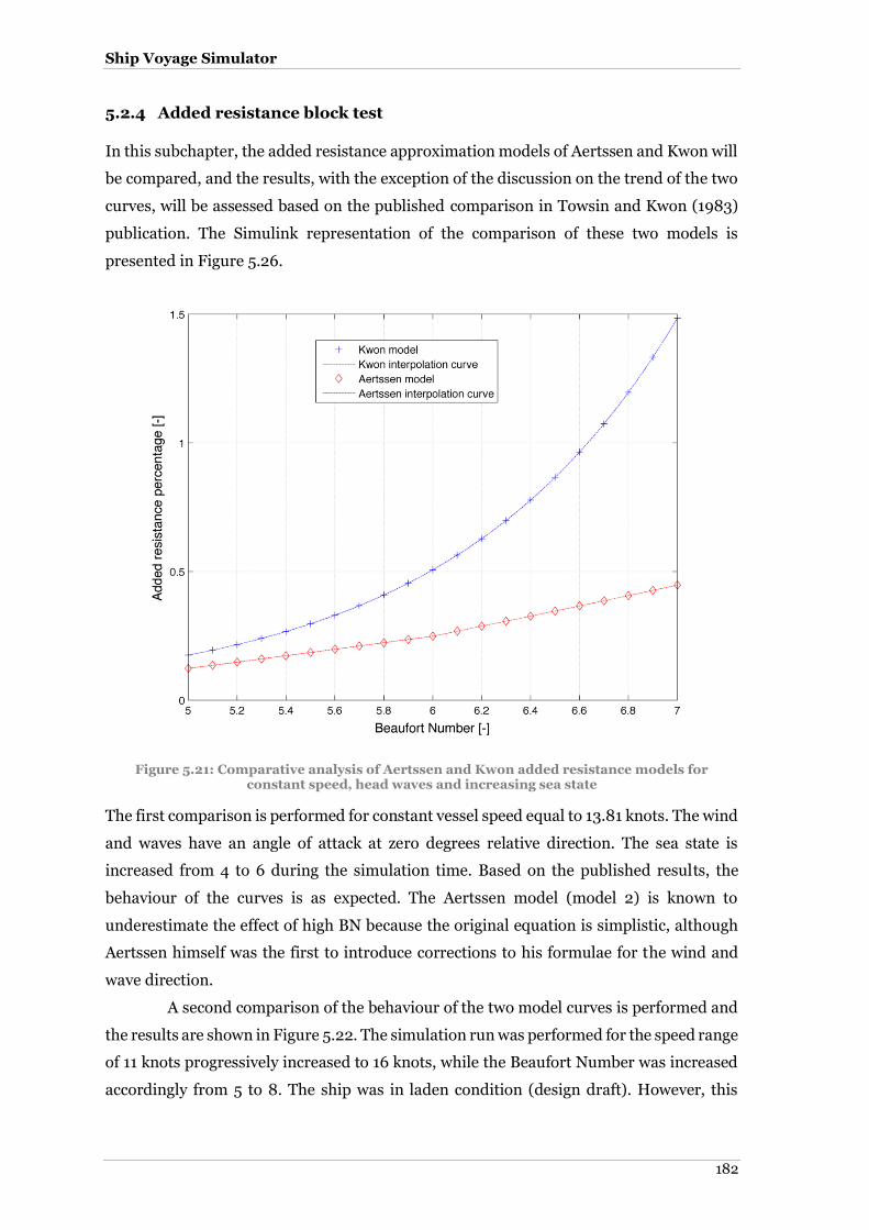
Ship Voyage Simulator
182
5.2.4 Added resistance block test
In this subchapter, the added resistance approximation models of Aertssen and Kwon will
be compared, and the results, with the exception of the discussion on the trend of the two
curves, will be assessed based on the published comparison in Towsin and Kwon (1983)
publication. The Simulink representation of the comparison of these two models is
presented in Figure 5.26.
Figure 5.21: Comparative analysis of Aertssen and Kwon added resistance models for constant speed, head waves and increasing sea state
The first comparison is performed for constant vessel speed equal to 13.81 knots. The wind
and waves have an angle of attack at zero degrees relative direction. The sea state is
increased from 4 to 6 during the simulation time. Based on the published results, the
behaviour of the curves is as expected. The Aertssen model (model 2) is known to
underestimate the effect of high BN because the original equation is simplistic, although
Aertssen himself was the first to introduce corrections to his formulae for the wind and
wave direction.
A second comparison of the behaviour of the two model curves is performed and
the results are shown in Figure 5.22. The simulation run was performed for the speed range
of 11 knots progressively increased to 16 knots, while the Beaufort Number was increased
accordingly from 5 to 8. The ship was in laden condition (design draft). However, this

Chapter 5
183
approach differs from the real vessel operation as, when the vessel exceeds Beaufort
number 7, the master alters vessel speed in order to avoid slamming and racing of the
engine. Moreover, when the ship sails into Beaufort number 8 and higher, the master
lowers the fuel admission lever in order to ease the ship motions and the deck wetness
(Aertssen and Sluys, 1972).
Figure 5.22: Comparative analysis of Towsin and Kwon and Aertssen models for head waves, increasing Beaufort number and progressively increased speed.
It can be extracted from Figure 5.22 that the two models have good accuracy when the ship
sails with increasing speed up to Beaufort number 6. In higher sea states, when the ship
increases its speed instead of performing voluntary speed loss, there is an equivalent speed
loss which is translated into added resistance. The 33% of the equivalent speed loss in BN
8 given by model 2 is precisely what the equation implies. Model 1 value is within the
expected range, allowing the conclusion that the shape and the range of added resistance
and speed loss values are valid. However, the potential error in high sea states due to the
uncertainty in statistical data is limited based on the time the ships spent in high sea states,
as seen in Table 5.11. Nevertheless, it is advisable for the simulator user to identify which
of the two models best describe the sea state by comparing with the actual total resistance
if on-board measurements using torque meters exist.
In order to finalise the test cases of added resistance, one more comparison is
performed to evaluate the added resistance approximation, using the Series 60 model
results dimensioned for the examined Post-Panamax vessel. For this test case, a voyage of

Ship Voyage Simulator
184
thirty-two days is selected. The dominating weather parameters, such as the wind force,
the sea state and the relative angle of attack for wind and waves, are obtained from the
examination of thirty-two ‘noon reports’ of the examined vessel. The daily mean vessel
speed and the mean daily reported Beaufort number are presented in Figure 5.23. Based
on the depicted values of this figure, it can be said that there is a voluntary speed loss when
the ship sailed in sea state 6 (Beaufort number 7). Concerning the values of added
resistance, Figure 5.24 and the detail of the latter figure presented in Figure 5.25 are
introduced.
Table 5.11: Percentage of sailing time in specific Beaufort numbers
Laden Voyage Ballast Voyage
Vessel 1 Vessel 2 Vessel 3 Vessel 1 Vessel 2 Vessel 3
BF ≤ 4 5.88% 12.50% 0.00% 6.45% 11.11% 0.00% 6.25%
BF = 5 76.47% 75.00% 75.00% 45.16% 0.00% 54.55% 25.00%
6 ≤ BF ≤ 7 17.65% 12.50% 25.00% 48.39% 88.89% 45.45% 68.75%
Figure 5.23: Daily mean Beaufort Number and vessel speed versus voyage day
It can be extracted from Figure 5.24 that there is an added resistance increase due to the
increase of sea state on the second day. After the third day, there is a significant drop in

Chapter 5
185
added resistance, which takes on negative values. Physically, the negative sign represents
the aid in the ship’s speed due to direction of the waves.
Figure 5.24: Added Resistance comparative analysis of Kwon and Series 60 methods
Figure 5.25: Detail of added Resistance comparative analysis of Kwon and Series 60 methods

Ship Voyage Simulator
186
On the fourth day, however, the vessel speed is increased and reaches the maximum
reported value, as seen in Figure 5.23, while the added resistance takes the maximum
absolute value at the same time, presenting the coherence of the reported data. The Kwon
model, however, is modelled in a way that does not permit the usage of negative or positive
signs, making the comparison more difficult.
Concerning the rest of the voyage, significant deviations occur on the eleventh day
and up to the fourteenth, as depicted in Figure 5.25. Taking into account the extreme
deviation of the Kwon model and the series 60 approximation for day twenty-seven to
thirty-two, it can be concluded that the connection of the vessel speed (or Froude number)
is the dominant parameter for the accuracy of the models. In addition, there is no
capability to extract secure conclusions, as the Kwon model is sensitive to the Beaufort
number value and to the vessel speed, while the tabular data of Series 60 approximation
is sensitive to the wave angle and the Beaufort number, and not so much to the Froude
number, as the model interpolates only between 0, 0.1, 0.2 Froude number values,
significantly reducing the model sensitivity in speed variations.
Figure 5.26: Simulink representation for added resistance comparative analysis
Added Resistance mean
model Block
Input
Blocks

Chapter 5
187
5.2.5 Non-linear optimisation test
The simulations were performed for the auxiliary loads of a Bulk carrier for a time period
of 24 hours. Primarily, the simulator was fed by an artificial load, which remains constant
for 2.4 hours, in order to validate the simulator’s ability to operate with initially depleted
batteries (Depth of Discharge 100%). The results are presented in a graphical way in Figure
5.27. In combination with Figure 5.28, it can be extracted that the battery is charged
(because of a rule based restriction, as the system prohibits the operation with State of
Charge less than 10%) and is followed by discharge and then by a charge. Meanwhile, in
order to meet the power demand, the Hybrid system engine alters its load, which is
depicted in blue in Figure 5.27. The percentage of this fluctuation is determined by the
ECMS strategy, which optimises the system operation in order to save energy for future
demand and thus minimise fuel consumption and emissions. Of crucial importance to the
outcome of the optimisation and the racing over batteries percentage is the installed
energy capacity. For the artificial load, the capacity was set to 2MWh. The selection energy
capacity of the storage medium is dependent on the engine auxiliary output and the study
of electric load analysis.
Figure 5.27: Comparison of Conventional, Hybrid engine outputs and battery power

Ship Voyage Simulator
188
Figure 5.28: Battery Depth of Discharge versus simulation time
Figure 5.28 denotes that the hybrid system is charging for 50% of the simulation time,
discharging for 40% and remains idle for 10% of the time. This graph denotes that the logic
criteria that accompany the optimisation algorithm do apply and constrain the
optimisation procedure in order to maintain the battery SoC close to the reference value,
which is 35%. However, the SoC reference is the minimum SoC that the system should
have at the end of the reference time. Based on this figure, the optimisation algorithm
applied energy to the battery, reaching, at the final time step, a SoC equal to 80%.
5.3 Implementation example – Simulation representation
In this section, the example of section 4.4 is implemented in the Simulink environment
using the blocks described in section 5.1.
The selected voyage is a 31 day ballast voyage from Hong Kong to Brazil. A data
file containing the vessel geometrical information for the sailing draft, the freeboard etc.
should be created and inserted to the simulator. The input data blocks are the source of
information for the simulation. Every output port is connected to its unique parameter
which is defined in a matrix form. As a result, the data file should provide the required
information in matrix structure. A sample matrix is depicted in Table 5.12, where the
information provided are the geometrical characteristics of the examined ship. Once this
process is completed, the unique parameters defining the voyage should be provided. The
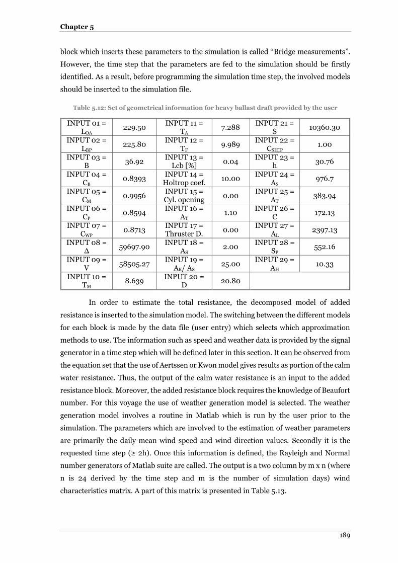
Chapter 5
189
block which inserts these parameters to the simulation is called “Bridge measurements”.
However, the time step that the parameters are fed to the simulation should be firstly
identified. As a result, before programming the simulation time step, the involved models
should be inserted to the simulation file.
Table 5.12: Set of geometrical information for heavy ballast draft provided by the user
INPUT 01 = LOA
229.50 INPUT 11 =
TA 7.288
INPUT 21 = S
10360.30
INPUT 02 = LBP
225.80 INPUT 12 =
TF 9.989
INPUT 22 = CSHIP
1.00
INPUT 03 = B
36.92 INPUT 13 =
Lcb [%] 0.04
INPUT 23 = h
30.76
INPUT 04 = CB
0.8393 INPUT 14 =
Holtrop coef. 10.00
INPUT 24 = AS
976.7
INPUT 05 = CM
0.9956 INPUT 15 = Cyl. opening
0.00 INPUT 25 =
AT 383.94
INPUT 06 = CP
0.8594 INPUT 16 =
AT 1.10
INPUT 26 = C
172.13
INPUT 07 = CWP
0.8713 INPUT 17 = Thruster D.
0.00 INPUT 27 =
AL 2397.13
INPUT 08 = Δ
59697.90 INPUT 18 =
AS 2.00
INPUT 28 = SP
552.16
INPUT 09 = V
58505.27 INPUT 19 =
AK/ AS 25.00
INPUT 29 = AH
10.33
INPUT 10 = TM
8.639 INPUT 20 =
D 20.80
In order to estimate the total resistance, the decomposed model of added
resistance is inserted to the simulation model. The switching between the different models
for each block is made by the data file (user entry) which selects which approximation
methods to use. The information such as speed and weather data is provided by the signal
generator in a time step which will be defined later in this section. It can be observed from
the equation set that the use of Aertssen or Kwon model gives results as portion of the calm
water resistance. Thus, the output of the calm water resistance is an input to the added
resistance block. Moreover, the added resistance block requires the knowledge of Beaufort
number. For this voyage the use of weather generation model is selected. The weather
generation model involves a routine in Matlab which is run by the user prior to the
simulation. The parameters which are involved to the estimation of weather parameters
are primarily the daily mean wind speed and wind direction values. Secondly it is the
requested time step (≥ 2h). Once this information is defined, the Rayleigh and Normal
number generators of Matlab suite are called. The output is a two column by m x n (where
n is 24 derived by the time step and m is the number of simulation days) wind
characteristics matrix. A part of this matrix is presented in Table 5.13.

Ship Voyage Simulator
190
Table 5.13: Wind speed regeneration matrix sample using Rayleigh distribution generator
Time segement
Day 1 Day 2 Day 3 Day 4 Day 5 Day 6 Day 7 Day 8
0-2 5.67 4.20 12.78 4.29 6.94 7.77 8.04 1.88
2 – 4 5.67 2.82 2.07 6.37 15.03 11.01 4.58 1.93
4 – 6 6.25 6.40 11.93 5.64 9.01 8.45 13.51 3.54
6 – 8 3.03 7.23 6.49 1.77 12.46 17.67 6.58 4.24
8 – 10 5.75 4.09 10.54 3.24 9.01 11.96 16.25 0.73
10 – 12 1.37 8.75 5.95 9.13 8.52 12.85 2.60 1.41
12 – 14 12.08 3.55 5.87 4.79 6.22 2.68 0.93 6.16
14 – 16 6.09 9.99 14.07 15.66 1.99 12.46 2.96 6.20
16 – 18 2.98 4.31 1.72 20.59 12.32 7.83 0.93 6.72
18 – 20 8.47 10.59 0.76 5.62 12.75 11.22 2.82 3.08
20 – 22 6.74 6.75 7.32 8.65 7.25 13.05 1.09 6.38
Using the mathematical representation of Chapter 4, the wind speed is transformed to
significant wave height. This vector is loaded to a signal generator, along with the speed
and the rest time variant user input parameters. Because the used mean added resistance
models require the Beaufort number in every time step, the significant wave height during
simulation is transformed to Beaufort number with a 2D lookup table (Beaufort number
versus significant wave height) which is derived from Table 4.3. Thus the added resistance
is estimated. The wind resistance is calculated by the dedicated block for wind induced
loads. The wind speed and direction are directly fed to the block without any
transformation. Moreover, the rest ship geometrical constants are also fed and the wind
resistance is approximated. Because a dedicated block for wind resistance is used, the
added resistance block calculates the effect of wind as well. Therefore, the added resistance
output is transformed so that the portion of added resistance due to wind loads is removed.
As a result, there is no double calculation of any contributing resistance factor to the total
ship resistance. Nevertheless, in order to account all the resistance values, the use of a
block which performes the algebraic sum of resistance components is required. The
Simulink offers an embedded block for this operation. Nonetheless, the added resistance
block has as output the added resistance as proportion of the calm resistance. Thus, the
added resistance due to waves is transformed from percentage of calm resistance to
absolute value by a simple multiplication and then is connected to the resistance combiner.
The total resistance is now defined. It should be also mentioned, that in every case that
algebraic summations between output values of different blocks, the use of combiners is
mandatory.
Eventually the fuel engine power and fuel consumption have to be simulated. In
order to connect the ship resistance with the required propulsive power, the use of
Propeller block is required. The block outputs are the required engine torque and the

Chapter 5
191
developed propeller thrust. This block has as inputs, the total ship resistance for given
speed and the hydrodynamic coefficients which describe the examined hull. In addition a
full set of propeller characteristics is required. The propeller characteristics are supplied
by the “input data blocks”. The dedicated input block is the “Ship Propeller Data” which is
illustrated in Figure 5.3. The hydrodynamic coefficients are supplied by the input data
model (user entry) or by the Holtrop-Mennen model, if the user selects this option. In case
that the Hollenbach method is used, the user has to supply through the data file the
hydrodynamic coefficients, otherwise the simulator cannot run. For this demonstration
scenario, the hydrodynamic coefficients were obtained from the towing tank tests and are
built in Simulink environment as 2D lookup tables with only input the vessel sailing speed
at each time step.
The governing equations of the propeller block are implemented using the S-
function format. By applying the mid-point method of numerical analysis the propeller
RPM are defined. The appropriate advance coefficient J is determined so the resistance
and thrust (accounting the losses) are equal, thus the ship can steam with the user
predefined speed. After identifying the propeller RPM and the required thrust and torque,
the main engine power is estimated prior to any transmission losses. The shaft losses are
user input and are defined when implementing the initial simulation data file.
According to the mathematical implementation, when the power profile is
determined by the Propeller block, the engine block is required so as to identify the fuel
consumption. The SFOC curve is implemented as a 2-D lookup table. The lookup table
represents the SFOC of the M/E versus engine load. Thus, the engine load should be
defined at every time step. This is estimated by a simple mathematical derivation of power
by the engine MCR (user entry at data file) using the mathematical basic design blocks of
Simulink. The corrections are made inside the S-Function. The fuel low calorific value, the
operating temperature are supplied by the user thought the input data file. Based on Figure
5.11, the engine block has many outputs which are reserved for future use. For example,
when the model is used by a Technical department of a maritime company which requests
information regarding the thermodynamic performance of the engine, these lookup tables
will depict the thermodynamic performance of the engine versus its loading. Thus, because
such information is not required in this thesis, this block will not be further analysed.
Finally, when the input and model blocks have been connected, and the
appropriate information display/save blocks have been defined and connected to the
appropriate block output ports, the simulation time step should be defined and so the
computer’s method for simulating the desired scenario.
In order to identify the simulation time step Figure 5.2 should be used. Based on
this figure, the calm water resistance model has a minimum response of 1 minute. The

Ship Voyage Simulator
192
added resistance of 1 hour and the wind induced loads less than 20 minutes. In order to
couple these models together and give correct results, the maximum response time is
selected. Thus, the first simulation time can be defined and is set to 1 hour. However, in
order to have a fully developed sea and the weather generator model to be valid, 2h
response time is required for this model. Thus the simulation time is at least defined to 2
hours. Regarding the engine model, the response time of the engine can be less than a
minute for short fluctuations or can be up to 30 minutes for progressive increase/ decrease
of load which can be overwritten by the crew if necessary. For this simulation, one minute
can be considered as a good average time. Regarding the propeller model two minutes
response time is acceptable time. Hence, the simulation time for this examined case is two
hours.
The problem is discrete and does not involve differential equations, thus a
discrete state solver which is fast and accurate can solve the mathematical equations of the
blocks. Regarding the total simulation time, the number of voyage hours should be divided
by 12 in order to get the discrete simulation time steps. This number is deducted by 1
because the simulation starts from step zero. (t=0). Once all the above have been
accomplished, the user can use sinks to have screen representation of the block outputs or
use the Matlab/ Simulink integration to save the output data to matrices. Using this
capability, the power profile is extracted from the Simulink environment and is saved to
predefined format and name data file inside a specific directory. The data file is a two
dimensional matrix which containts the power requiremernt in one row and in the second
row the simulation time step. Then this matrix is imported by the Optimisation algorithm.
The optimisation algorithm was implemented in Matlab due to the non-linear
form and because of the time consuming process for it to be implementeded in the
Simulink environment. Furthermore, this would also allow power profiles derived from
shipboard measurements or laboratory tests.
The results of the implementation example concerning the voyage simulation are
presented in section 6.1.2 while the optimisation results for the acquired and simulated
power profiles in section 6.2.

Chapter 5
193
5.4 Chapter summary
This chapter presented the simulation block implementation of the mathematical
equations presented in Chapter 4. The key characteristics of the simulator package and the
advantages of the graphical programming have been discussed. It was found that the
adoption of signal flows and major block leads to non-complex models which are more
convenient for simulation expansion while maintaining a low risk of programming errors.
Furthermore, it was found that the calm water resistance in design draft is better
approximated by the Hollenbach method which is more up to date and is based on the
statistical analysis of a large number of modern hull forms.
Moreover, the Blendermann method was also selected to describe the wind
induced loads as it is a more up to date method.
Regarding the added resistance due to wind and waves, the method of Aertssen
or Kwon is selected. The latter method compared to the Grigoropoulos et al. (2001)
approach was found to be more accurate in the method’s applicability range. Thus, the
calculations are based on Kwon (2008) model with the exception when the introduced
error to the calculations is high (large power difference when comparing measured data at
similar conditions with the simulated ones and when continuous overloading of M/E is
present, something that is not possible to happen regurarily); hence the modest approach
of Aertssen is selected.
Due to the absence of RAO data which are more accurate than a daily mean
approximation procedure, this thesis demonstrated a way to regenerate environmental
conditions in order to apply a mean added resistance model, resulting in fluctuating
environmental parameters per day. This method regenerates the environmental
parameters at two-hour intervals, using weather forecasting formulae and by applying the
assumption that sea spectra, which describe the current, are only valid for up to two-hour
periods. A Rayleigh statistical distribution was used for wind speed, and a Normal
distribution around the reported mean value was also implemented for wind direction.
This procedure resulted in more accurate than the daily mean model and introduced
significant less uncertainty than the Grigoropoulos et al. (2001) proposal.
For the engine propeller interaction, the Wageningen B-series approximation has
good accuracy compared to the model test data. However, because the effect in engine
RPM cannot be neglected, for the simulation purposes the model test data should be used.
Concerning the test case of the non-linear optimisation, the ECMS strategy was
adopted. It was found that the algorithm performs power split between the prime movers
and the battery system. In addition, the logic criteria for charging conditions are always
met and the algorithm converges to a global minimum, resulting in fuel savings.

Ship Voyage Simulator
194
On the scope of the above, the simulation blocks are considered accurate;
therefore the simulator can be used in combination with the optimisation algorithm to
solve powering scenarios. The results of voyage cases along with the optimisation of power
vectors for both propulsive and auxiliary loads are given in the next Chapter 6.

Chapter 6
195
6 Simulation and Optimisation Results
This chapter presents the results of voyage simulation cases and uses simulator outputs to
assess the Hybrid power layouts using the implemented ECMS optimisation algorithm.
The first part demonstrates the accuracy of the ship voyage simulator compared to the ‘as
measured’ data obtained from the shipping company. Various runs have been performed
at this stage and a variation of the parameters is also presented for clarification purposes.
The second part of this chapter contains the optimisation outcomes concerning the Diesel
Hybrid power system. Three examined layouts are presented.
6.1 Ship Voyage simulation
For the ship simulator test case scenarios, voyage conditions are modelled based on the
vessels’ daily performance reports. The total mean daily power (Ptotal) was calculated by the
ship simulator using the models described in Chapter 4. This power is determined by the
Thrust-Resistance match for self-propelled ships sailing with constant speed setting. Thus,
Ptotal is the required shaft power to achieve the reported speed at a specific sea state. The
primary source of engine loading is obtained by the simulator, with the relevant Simulink
representation is illustrated in Figure 6.1. The selection of the suitable mathematical
models and simulation blocks was described in sections 4.4 and 5.3 respectively. Figure
6.1 depicts the layout of the simulation blocks, the input data and signal generator blocks
and their interconnections using signal arrows in simulation environmnent. Display/ save
blocks can also found in this figure. The outline of this Figure is always specific as the
Simulink utilises the principles of graphical programming. Always from the left hand side
the user defined information is located. To the right hand side, the simulation outputs are
found.
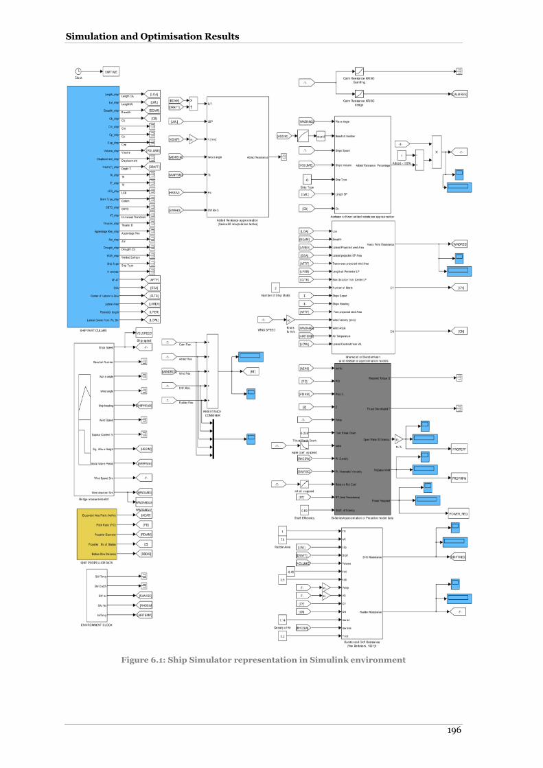
Simulation and Optimisation Results
196
Figure 6.1: Ship Simulator representation in Simulink environment

Chapter 6
197
Voyage simulation using 24 hour time step
For the conventional configuration, six voyages have been implemented in the simulation
environment. For the needs of the simulation, mean 24h values are inserted to the
simulator. The accuracy of reported data relies on the ship’s master. However, during the
sampling period, the data consistency was checked and in cases where errors exceed the
5% of the sampled data, the voyage was rejected and re-sampling was made.
Given the environmental parameters, the corrected SFOC can be determined and
the total fuel consumption to be estimated. For the 6 voyages where details can be found
in Table 6.1, comparison between actual fuel consumption and reported fuel consumption
is made. For demonstration purposes a thirty-two day laden voyage between Australia
(Dalrymple Bay coal station) and Italy (Port Taranto) is presented in detail. The ship sailed
9,535 sea miles. The ‘as measured’ fuel consumption for the main engine was equal to
1359.1 tonnes.
Table 6.1: Ship Simulation examined voyages and cargo quantity present
Ship Departure
Port Arrival Port
Distance (sea miles)
Cargo Type Quantity
(MT)
Vessel 1 Rio Grande Marin 5168
Soya Beans Milled
60600
Hong Kong Tubarao 9435 Ballast 39063
Vessel 2 Tubarao Amsterdam 5045 Grains 80000
Port Talbot Port Cartier 2610 Ballast 39060
Vessel 3
Dalrymple Bay
Taranto 9535 Coal 89524
Luoyan Dalrymple bay 3906 Ballast 39121 Rio Grande Marin 5168 Ballast 40500
For the resistance approximation in laden voyage, for increased accuracy reasons, the full
scale correlated results from ship model tests were used. The runs were performed for the
case that the ship sailed at constant speed in any faced sea state.
The actual propeller performance data was selected instead of the Wageningen B-
series approximation, for the same reason. For the approximation of added resistance due
to waves, the formulae of Aertssen instead of Kwon (2008) are selected because they insert
a modest approach to the effect of added resistance and because the simulation resulted in
continuous engine overload a fact that indicates that the Kwon model overestimated the
added resistance significantly.
The simulated resistance breakdown is presented in Figure 6.2. It can be
identified from this figure that the largest percentage of the resistance is held by the calm
water resistance. The wind resistance seems to reduce the total resistance over a large
number of simulated days as the wind hits the vessel from the quarter or astern.
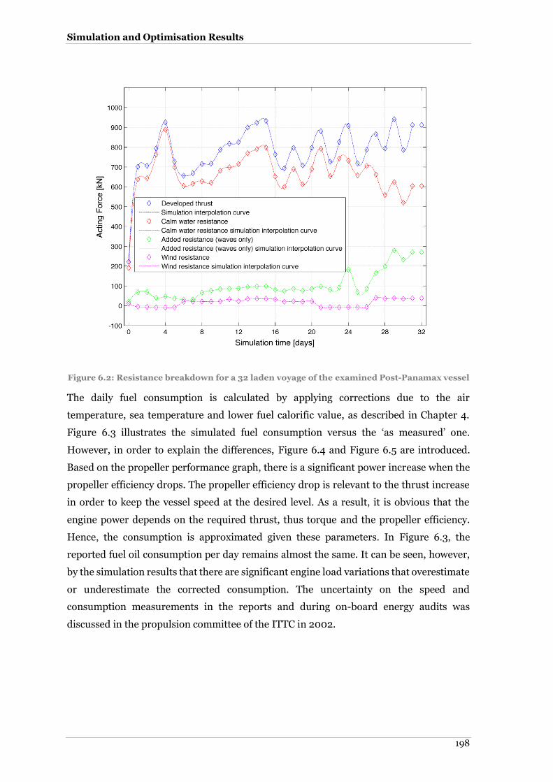
Simulation and Optimisation Results
198
Figure 6.2: Resistance breakdown for a 32 laden voyage of the examined Post-Panamax vessel
The daily fuel consumption is calculated by applying corrections due to the air
temperature, sea temperature and lower fuel calorific value, as described in Chapter 4.
Figure 6.3 illustrates the simulated fuel consumption versus the ‘as measured’ one.
However, in order to explain the differences, Figure 6.4 and Figure 6.5 are introduced.
Based on the propeller performance graph, there is a significant power increase when the
propeller efficiency drops. The propeller efficiency drop is relevant to the thrust increase
in order to keep the vessel speed at the desired level. As a result, it is obvious that the
engine power depends on the required thrust, thus torque and the propeller efficiency.
Hence, the consumption is approximated given these parameters. In Figure 6.3, the
reported fuel oil consumption per day remains almost the same. It can be seen, however,
by the simulation results that there are significant engine load variations that overestimate
or underestimate the corrected consumption. The uncertainty on the speed and
consumption measurements in the reports and during on-board energy audits was
discussed in the propulsion committee of the ITTC in 2002.

Chapter 6
199
Figure 6.3: Simulated versus ‘as measured’ fuel consumption for a 32 laden voyage of the examined Post Panamax vessel
Based on this sample, it can be concluded that, although the total simulated consumption
is underestimated by 56.35 tonnes or 4.14% of the total fuel bill, the daily differences have
significant dissimilarities. In order to identify further differences between the simulator
estimations and the ‘as measured’ fuel consumption, five more voyages have been included
in the calculation. The results corresponding to the already presented voyage are
summarised in Table 6.2. The negative sign denotes that there is an underestimation of
the fuel consumption.
Table 6.2: Simulated versus the ‘as measured’ fuel consumption for all vessels and voyages
Laden Voyage Ballast Voyage
Vessel 1 Vessel 2 Vessel 3 Vessel 1 Vessel 2 Vessel 3 Simulated
Fuel consumption
616.11 614.07 1302.70t 978.45t 276.75t 390.22t 498.66t
Measured fuel
consumption 653.40 642.20 1359.10t 1206.80t 354.60t
438.20t 594.40t
Fuel difference
-37.29 -28.13 -56.35t -228.35 -77.85t -47.98t -95.74t
Percentage difference
-5.71% -4.38% -4.14% -18.92% -21.95% -10.95% -16.11%
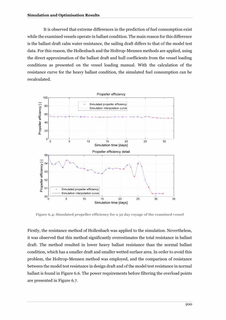
Simulation and Optimisation Results
200
It is observed that extreme differences in the prediction of fuel consumption exist
while the examined vessels operate in ballast condition. The main reason for this difference
is the ballast draft calm water resistance, the sailing draft differs to that of the model test
data. For this reason, the Hollenbach and the Holtrop-Mennen methods are applied, using
the direct approximation of the ballast draft and hull coefficients from the vessel loading
conditions as presented on the vessel loading manual. With the calculation of the
resistance curve for the heavy ballast condition, the simulated fuel consumption can be
recalculated.
Figure 6.4: Simulated propeller efficiency for a 32 day voyage of the examined vessel
Firstly, the resistance method of Hollenbach was applied to the simulation. Nevertheless,
it was observed that this method significantly overestimates the total resistance in ballast
draft. The method resulted in lower heavy ballast resistance than the normal ballast
condition, which has a smaller draft and smaller wetted surface area. In order to avoid this
problem, the Holtrop-Mennen method was employed, and the comparison of resistance
between the model test resistance in design draft and of the model test resistance in normal
ballast is found in Figure 6.6. The power requirements before filtering the overload points
are presented in Figure 6.7.
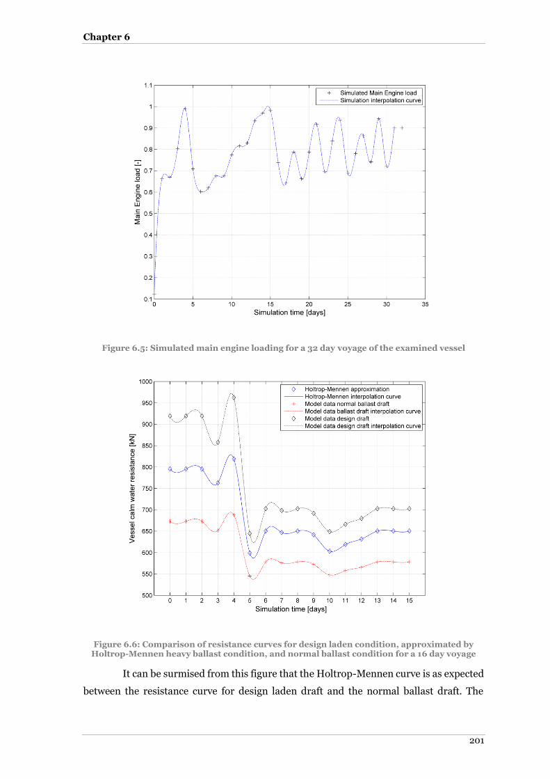
Chapter 6
201
Figure 6.5: Simulated main engine loading for a 32 day voyage of the examined vessel
Figure 6.6: Comparison of resistance curves for design laden condition, approximated by Holtrop-Mennen heavy ballast condition, and normal ballast condition for a 16 day voyage
It can be surmised from this figure that the Holtrop-Mennen curve is as expected
between the resistance curve for design laden draft and the normal ballast draft. The
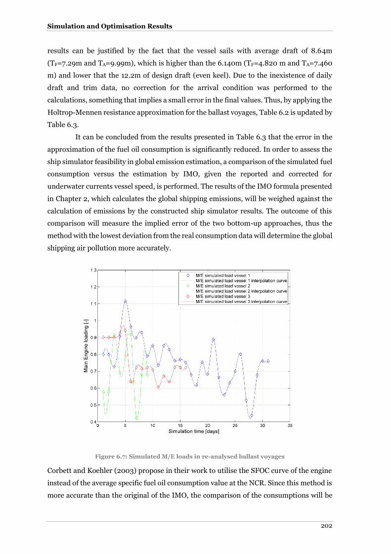
Simulation and Optimisation Results
202
results can be justified by the fact that the vessel sails with average draft of 8.64m
(TF=7.29m and TA=9.99m), which is higher than the 6.140m (TF=4.820 m and TA=7.460
m) and lower that the 12.2m of design draft (even keel). Due to the inexistence of daily
draft and trim data, no correction for the arrival condition was performed to the
calculations, something that implies a small error in the final values. Thus, by applying the
Holtrop-Mennen resistance approximation for the ballast voyages, Table 6.2 is updated by
Table 6.3.
It can be concluded from the results presented in Table 6.3 that the error in the
approximation of the fuel oil consumption is significantly reduced. In order to assess the
ship simulator feasibility in global emission estimation, a comparison of the simulated fuel
consumption versus the estimation by IMO, given the reported and corrected for
underwater currents vessel speed, is performed. The results of the IMO formula presented
in Chapter 2, which calculates the global shipping emissions, will be weighed against the
calculation of emissions by the constructed ship simulator results. The outcome of this
comparison will measure the implied error of the two bottom-up approaches, thus the
method with the lowest deviation from the real consumption data will determine the global
shipping air pollution more accurately.
Figure 6.7: Simulated M/E loads in re-analysed ballast voyages
Corbett and Koehler (2003) propose in their work to utilise the SFOC curve of the engine
instead of the average specific fuel oil consumption value at the NCR. Since this method is
more accurate than the original of the IMO, the comparison of the consumptions will be

Chapter 6
203
based on the simulated engine loading and the approximated engine loading. To estimate
the fuel consumption, each loading will be multiplied by the corrected SFOC and by the
engine MCR times the operational time. Given that an average fuel emission factor is used,
there will be no presentation of CO2 emissions, as the latter can be approximated easily, as
described in chapter 2. Thus, for the ballast voyage of vessel 1, the simulation reanalysis
showed that the simulator underestimated the total fuel oil consumption by 3.93%.
Table 6.3: Re-analysis of the ballast voyage fuel consumptions
Ballast voyage Re-analysis of ballast voyage
Vessel 1 Vessel 2 Vessel 3 Vessel 1 Vessel 2 Vessel 3 Simulated
Fuel consumption
978.45t 276.75t 390.22t 498.66t
1159.28t 307.43t 461.50t 600.44t
Measured fuel
consumption 1206.80t 354.60t
438.20t 594.40t
1206.80t 354.60t 438.20t 594.40t
Fuel difference
-228.35 -77.85t -47.98t -95.74t
-47.52 -47.17 23.30t 6.04t
Percentage difference
-18.92% -21.95% -10.95% -16.11%
-3.93% -13.30% 5.32% 1.02%
By applying the approximation of engine loading given the only the corrected
vessel speed, the IMO formula resulted in overestimation of the fuel consumption by
8.59%. For the first ballast voyage of vessel 3, the implied error by the IMO formula is
8.63% (overestimation), while the implied error by the ship simulator is 5.32%
(overestimation). It can be extracted by the comparison that both approaches introduce
uncertainty to the calculation but the total error is lower than the top down approach.
Moreover, the ship simulator proved to determine with more accuracy the actual
consumed fuel by applying a day-to-day energy approach.
Voyage simulation using 2h time step
In this section, the results of the demonstration test case which was presented in sections
4.4 and 5.3 are given. The selected voyage is a 31 day ballast voyage. Because only the daily
mean environmental parameters were known, the weather generation model is applied.
For the purposes of the simulation, there is no voluntarily speed loss due to bad weather
and the speed remains constant as per the performance report. In cases where the engine
loading exceeds 100%, the result is filtered and neglected, as there is no physical meaning
to this value, since the master always reduces speed to avoid engine overloading and
excessive ship motions. The simulated engine loading is presented in Figure 6.8 and the
speed setting versus the significant wave height is presented in Figure 6.9.

Simulation and Optimisation Results
204
Figure 6.8: Simulated Main Engine loading using 2h weather generation model
Based on the graph depicted in Figure 6.8, it can be said that the engine is overloaded in
25 samples over the generated 373, a fact that supports the initial assumption that the
vessel does not alter its speed when sea state increases during each voyage day.
Figure 6.9: Vessel speed and significant wave height correlation applying 2h weather generation model

Chapter 6
205
Concerning the first peak of engine loading around the 45th two-hour segment, the vessel
speed is not reduced when the vessel faces waves with a significant wave height value
around 5.2 m. Nevertheless, in the extreme weather around the 32oth sample, the master
reduces the speed and the outcome on the engine loading is obvious in Figure 6.8. In order
to finalise the picture on the effect of environmental parameters, the direction of waves is
presented in Figure 6.10. This figure demonstrates why the effect of waves is greater in the
peak engine loads. This is explained by the fact that head waves dramatically increase the
propulsive power for constant speed, while the abeam or astern waves aid the surge
forward movement, reducing the total propulsive power. Taking into account the
aforementioned information, the simulator is expected to overestimate the total fuel
consumption due to the discussed engine overloading. Consequently, the simulated fuel
oil consumption equals to 1240.1 tonnes meaning, 33 tonnes more consumed fuel or 2.75%
implied error with this working procedure.
Figure 6.10: Simulated Wind direction using 2h weather generation model
This error will potentially decrease with better tuning of the simulator, by supplying a
model to alter the speed based on the simulated significant wave height. Nonetheless, the
approximation of fuel consumption yields to a very small deviation from the actual fuel
consumption and the results are closer than the IMO study method.
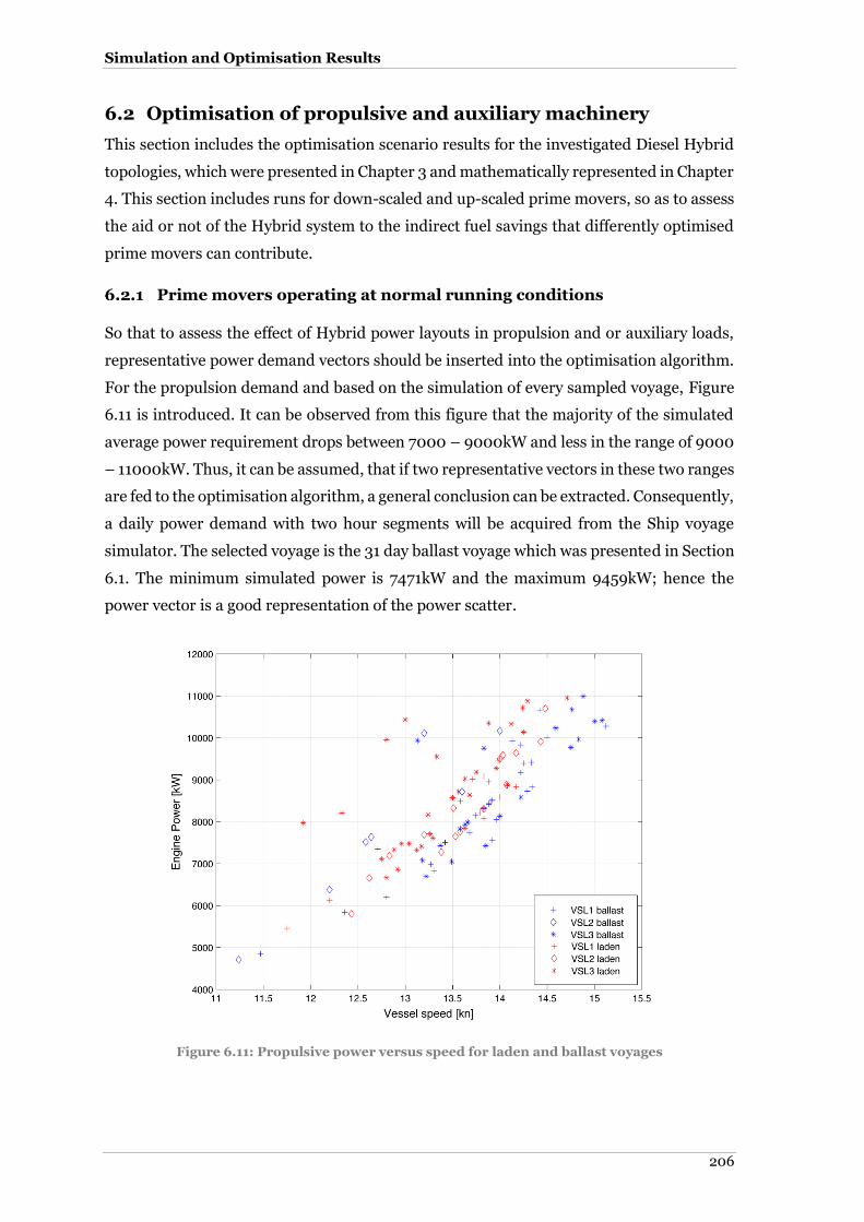
Simulation and Optimisation Results
206
6.2 Optimisation of propulsive and auxiliary machinery
This section includes the optimisation scenario results for the investigated Diesel Hybrid
topologies, which were presented in Chapter 3 and mathematically represented in Chapter
4. This section includes runs for down-scaled and up-scaled prime movers, so as to assess
the aid or not of the Hybrid system to the indirect fuel savings that differently optimised
prime movers can contribute.
Prime movers operating at normal running conditions
So that to assess the effect of Hybrid power layouts in propulsion and or auxiliary loads,
representative power demand vectors should be inserted into the optimisation algorithm.
For the propulsion demand and based on the simulation of every sampled voyage, Figure
6.11 is introduced. It can be observed from this figure that the majority of the simulated
average power requirement drops between 7000 – 9000kW and less in the range of 9000
– 11000kW. Thus, it can be assumed, that if two representative vectors in these two ranges
are fed to the optimisation algorithm, a general conclusion can be extracted. Consequently,
a daily power demand with two hour segments will be acquired from the Ship voyage
simulator. The selected voyage is the 31 day ballast voyage which was presented in Section
6.1. The minimum simulated power is 7471kW and the maximum 9459kW; hence the
power vector is a good representation of the power scatter.
Figure 6.11: Propulsive power versus speed for laden and ballast voyages
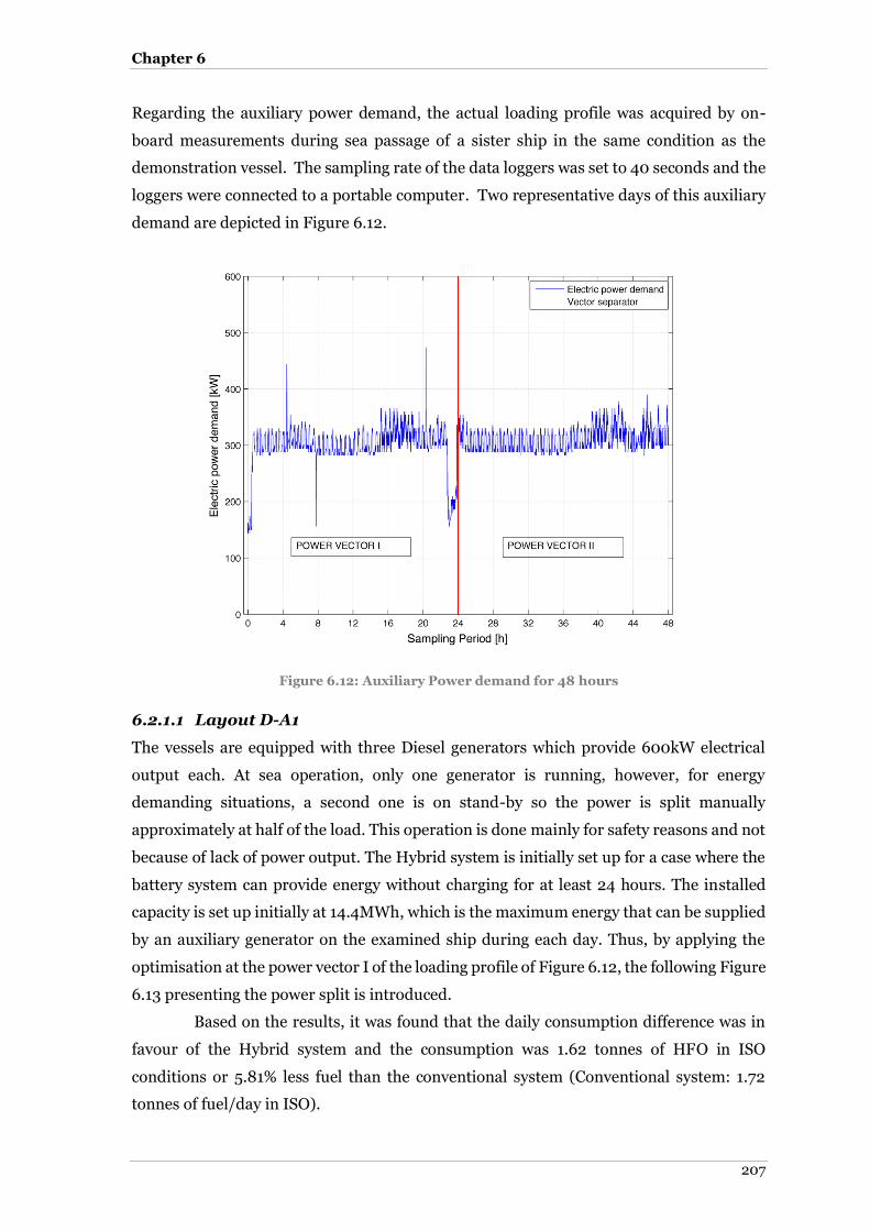
Chapter 6
207
Regarding the auxiliary power demand, the actual loading profile was acquired by on-
board measurements during sea passage of a sister ship in the same condition as the
demonstration vessel. The sampling rate of the data loggers was set to 40 seconds and the
loggers were connected to a portable computer. Two representative days of this auxiliary
demand are depicted in Figure 6.12.
Figure 6.12: Auxiliary Power demand for 48 hours
6.2.1.1 Layout D-A1
The vessels are equipped with three Diesel generators which provide 600kW electrical
output each. At sea operation, only one generator is running, however, for energy
demanding situations, a second one is on stand-by so the power is split manually
approximately at half of the load. This operation is done mainly for safety reasons and not
because of lack of power output. The Hybrid system is initially set up for a case where the
battery system can provide energy without charging for at least 24 hours. The installed
capacity is set up initially at 14.4MWh, which is the maximum energy that can be supplied
by an auxiliary generator on the examined ship during each day. Thus, by applying the
optimisation at the power vector I of the loading profile of Figure 6.12, the following Figure
6.13 presenting the power split is introduced.
Based on the results, it was found that the daily consumption difference was in
favour of the Hybrid system and the consumption was 1.62 tonnes of HFO in ISO
conditions or 5.81% less fuel than the conventional system (Conventional system: 1.72
tonnes of fuel/day in ISO).

Simulation and Optimisation Results
208
Figure 6.13: Power split between Auxiliary Engines and batteries of energy capacity of
14.4MWh and comparison with the conventional system
However, as it is observed from the power demand figure, the maximum instantaneous
peak load was 450kW, hence the daily demand is around 10MWh. In addition due to the
extreme amount of installed energy in batteries and restrictions in carrying capacity of the
vessel, a scenario with the same demand profile was performed, but with reduced energy
capacity in the battery. A 10 – 15% of the capacity of the generator can be considered
sufficient for load levelling purposes. Thus, the second run involves capacity equal to
2MWh. The power split for this scenario is depicted in Figure 6.14
It was found that the consumption of the hybrid system was lower than the
conventional, but the savings are almost negligible (0.0083 tonnes less fuel or 0.48%
savings). Figure 6.14 depicts the power split between the battery and the auxiliary engine.
It can be surmised from Figure 6.14 that, for specific loads, the usage of the hybrid system
is not cost effective. Because of this finding, the engines are switching on and off and the
power split is performed either by the battery only or by the auxiliary engine only. In
addition, the observed non-stable power split is explained by the pairing of the Auxiliary
engine, the reduced size of the battery bank and the implementation of the logic
optimisation criteria. Consequently, the regular switch from idle to ~50% load of each
generator engine is a product of the fast depletion of the battery bank and the existence of
non-favourable charging conditions which do not meet the rule based optimisation criteria
(the cycling over batteries after 16th hour reaches 0%). Because the rule set for charging

Chapter 6
209
cannot escape from the loop of no charging solution, the logic has been altered.
Furthermore, more battery capacities have been investigated. The results indicate that the
saving percentage is improved and the battery is charged by the 16th hour and onwards
with increased rate as the tsim approaches the tref, due to the existence of lambda coefficient.
Figure 6.14: Power split between Auxiliary Engines and batteries of energy capacity 2MWh
and comparison with the conventional system
Three more battery capacities are investigated which are presented in Table 6.4 along with
the fuel saving percentage. The capacity of the 7MWh corresponds approximately to a
power equivalent of ~300kW for 24 hours, the 10MWh for ~450kW and the 4MWh is a
30% storage capacity of the maximum required energy per day.
Table 6.4: Effect of logic and installed capacity on the amount of fuel savings
Battery installed capacity [MWh]
Auxiliary fuel savings with logic improvements [-]
2 0.84% from 0.48%
4 2.64%
7 4.38%
10 5.57%
14.4 6.19% from 5.81%

Simulation and Optimisation Results
210
The saving percentage follows a quadratic curve (shown in Table 6.1) which curves
downwards and remains almost flat when the battery capacity reaches 14.4 MWh. The
reason for the convex form is that when the installed energy exceeds the daily requirement,
the effect of the larger battery bank only reduces the discharging/ charging current per
battery string which is already ultra-low, thus the effect is negligible over a 24h examined
period.
It can be observed from Table 6.4 that the rule based optimisation is affected by
the set applied logic criteria for charging. In addition, it is stated in Dedes et al. (2012a)
that the time step is of crucial importance on the feasibility of the Hybrid power system.
Given these parameters and taking into account that in layout D-C, the propulsion vector
has 2h sample rate, the auxiliary load power demand is transformed to a 2h mean vector.
The process involves the sampling of 180000 40sec values and exports a smaller set of
data which correspond to 2 hour mean power demands. Hence, the charging parameters
are altered. The reference time is reduced from 72h to 48h and 24h respectively. The
reference time affects the lambda coefficient, thus the charging percentage and the
charging logic. For all the cases, the logic improvements which were explained before
apply. The following Table 6.5 presents these effects on a 24h power vector.
Table 6.5: Effect of tref and sampling time in savings percentage for 24h sample
Case Capacity
24h vector, 2h sample rate, tref = 72h
24h vector, 2h sample rate, tref = 48h
24h vector, 2h sample rate, tref = 24h
2MWh 0.53% 0.52% 0.45% 4MWh 2.62% 2.94% -0.60% 7MWh 4.88% 4.91% 1.90%
10MWh 5.52% 5.52% 5.52%
14.4MWh 5.70% 5.70% 5.70%
It can be observed from Table 6.5 that the 2h mean power vector underestimates the
savings in cases where the charging effect is of vital importance. The main reason is that
given the power demand, the battery SoC may not be sufficient to cover the power for this
specific time, but be available for a shorter time, thus the simulation constraints which
have to be satisfied during the time step, reject the optimum solution which is to absorb
power from the battery bank. In cases were the simulation step is smaller, the decisions of
the optimisation algorithm have a lower influence on the drain/ charge rate of the battery
system, yielding to a more global optimised solution, as non-favourable conditions are
present for a shorter time than before and vice versa. Yet, the time division should be made
in accordance with the principle assumption that the system is operating in quasi-steady
conditions.
The reference time and the initial state of charge also alter significantly the
savings percentage as the lambda coefficient (described in equation 4.10.1) is increased
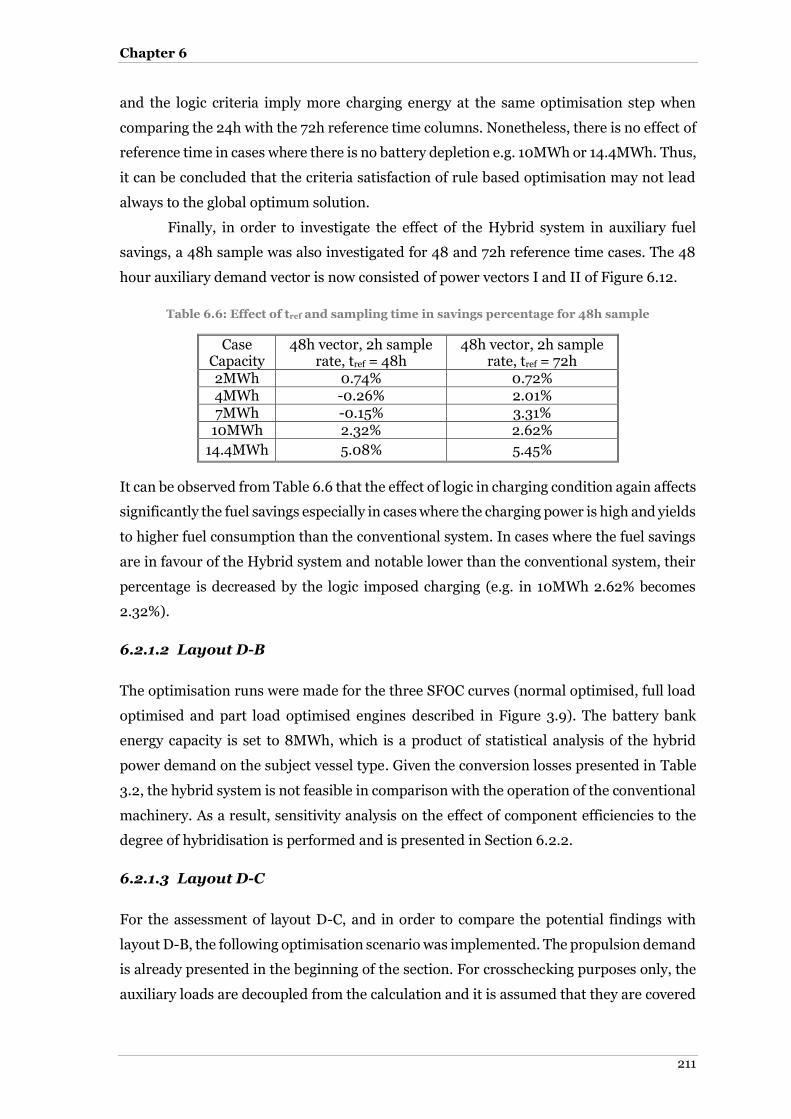
Chapter 6
211
and the logic criteria imply more charging energy at the same optimisation step when
comparing the 24h with the 72h reference time columns. Nonetheless, there is no effect of
reference time in cases where there is no battery depletion e.g. 10MWh or 14.4MWh. Thus,
it can be concluded that the criteria satisfaction of rule based optimisation may not lead
always to the global optimum solution.
Finally, in order to investigate the effect of the Hybrid system in auxiliary fuel
savings, a 48h sample was also investigated for 48 and 72h reference time cases. The 48
hour auxiliary demand vector is now consisted of power vectors I and II of Figure 6.12.
Table 6.6: Effect of tref and sampling time in savings percentage for 48h sample
Case Capacity
48h vector, 2h sample rate, tref = 48h
48h vector, 2h sample rate, tref = 72h
2MWh 0.74% 0.72% 4MWh -0.26% 2.01% 7MWh -0.15% 3.31%
10MWh 2.32% 2.62%
14.4MWh 5.08% 5.45%
It can be observed from Table 6.6 that the effect of logic in charging condition again affects
significantly the fuel savings especially in cases where the charging power is high and yields
to higher fuel consumption than the conventional system. In cases where the fuel savings
are in favour of the Hybrid system and notable lower than the conventional system, their
percentage is decreased by the logic imposed charging (e.g. in 10MWh 2.62% becomes
2.32%).
6.2.1.2 Layout D-B
The optimisation runs were made for the three SFOC curves (normal optimised, full load
optimised and part load optimised engines described in Figure 3.9). The battery bank
energy capacity is set to 8MWh, which is a product of statistical analysis of the hybrid
power demand on the subject vessel type. Given the conversion losses presented in Table
3.2, the hybrid system is not feasible in comparison with the operation of the conventional
machinery. As a result, sensitivity analysis on the effect of component efficiencies to the
degree of hybridisation is performed and is presented in Section 6.2.2.
6.2.1.3 Layout D-C
For the assessment of layout D-C, and in order to compare the potential findings with
layout D-B, the following optimisation scenario was implemented. The propulsion demand
is already presented in the beginning of the section. For crosschecking purposes only, the
auxiliary loads are decoupled from the calculation and it is assumed that they are covered

Simulation and Optimisation Results
212
by one of the three auxiliary generators. The efficiencies of Hybrid components are
described in Table 3.2. The battery energy capacity is set to 8MWh and the MCR of the
PTO/PTI system equals 600kW. The Main Engine is optimised for part load operation.
Table 6.7 presents the power split of the propulsion and auxiliary components for
layout D-C. The results indicate that, due to conversion losses, the battery system remains
idle. Nonetheless, the existence of the PTO/PTI system contributes to fuel savings, which,
for the given propulsion demand vector, amount to 7.23% of the fuel bill. The equivalent
fuel savings do not take into account the potential savings due to the part load optimisation
when compared to the normal optimisation.
Table 6.7: Power Split for layout D-C system for propulsive load demand
Simulation time [h]
Battery Output [kW]
M/E load [-]
A/E 1 load [-]
A/E 2 load [-]
A/E 3 load [-]
1 0 82.30% 100% 0 0 2 0 66.49% 100% 0 0 3 0 69.87% 100% 0 0 4 0 81.64% 100% 0 0 5 0 69.02% 100% 0 0 6 0 65.44% 100% 0 0 7 0 81.48% 100% 0 0 8 0 69.16% 100% 0 0 9 0 66.11% 100% 0 0 10 0 66.84% 100% 0 0 11 0 69.60% 100% 0 0 12 0 69.02% 100% 0 0
The operating principle of Hybrid layout D-C is depicted in Figure 6.15. The total fuel bill
is the multiplication of SFOC and the total kW. For this scenario, equations (6.2.1) and
(6.2.2) explain the optimisation algorithm solution.
/ / / / / /M E M E A E A E M E M ESFOC P SFOC P SFOC P (6.2.1)
The following constraint applies for the power split:
/ / /M E M E A EP P P (6.2.2)
The SFOC is load dependent, thus, if the engine operates at a less efficient point, the total
amount of kW is produced inefficiently. Using the PTO system, the extra kW are produced
in a far more inefficient way, although the remaining kW are produced in a more efficient
way, leading to fuel consumption savings and not to power savings. The difference of SFOC
is clear if Figure 3.8 and Figure 3.9 are compared for given loads. For the examined case,
the conventional system fuel consumption is 67.26 tonnes in ISO conditions, while for the
proposed layout D-C Hybrid system; fuel consumption for propulsion is 62.40 tonnes in
ISO (total difference of 4.86 tonnes HFO). Figure 6.15 explains that in cases where the ship

Chapter 6
213
is required to maintain a predefined speed constant, the RPM of the propeller need to
increase in order to match the total resistance with the produced thrust (accounting the
wake friction and thrust deduction factors).
Figure 6.15: Operating principle of D-C Hybrid power layout
However, instead the engine to increase load, M/E will operate in constant power mode
and the difference is covered by the PTO/PTI system. Nonetheless, in an ideal solution,
the best fuel consumption would be achieved if the M/E working point would be at the fuel
optimisation point set up by the engine manufacturer.
In continuation of the layout D-C assessment, auxiliary loads of Figure 6.12
transformed in 2hour mean segments are inserted to the optimisation algorithm. The
system leads to fuel savings of 7.23% for the propulsive loads and 5.38% for the auxiliary
loads. During this operation, the system is absorbing an amount of energy from the
batteries for the cover of auxiliary demand. Nevertheless, because the principle of
optimisation does not take into account the overall simulation picture, it identifies the best
solution of a specific time step (Guzzella and Sciarretta, 2005), ignoring a different voyage
minimum that could be found using Dynamic Programming. The power split and the
battery DoD for this scenario are given in Table 6.8. It should be noted that the DoD of the
battery at the initial time step is of great importance to the amount of fuel savings. The
charging criteria may lead the optimisation algorithm to non-optimum solutions when

Simulation and Optimisation Results
214
compared to the baseline system, but to lead to best fit to purpose solutions in terms of
criteria satisfaction.
Table 6.8: Power Split for layout D-C system for propulsive load and auxiliary demand
Simulation time [h]
Battery Output [kW]
M/E load [-]
A/E 1 load [-]
A/E 2 load [-]
A/E 3 load [-]
Battery DoD [%]
1 306.73 82.30% 100% 0 0 7.67% 2 330.05 66.49% 100% 0 0 15.92% 3 314.61 69.87% 100% 0 0 23.78% 4 324.95 81.64% 100% 0 0 31.91%
5 345.30 69.02% 100% 0 0 40.54%
6 299.37 65.44% 100% 0 0 48.03%
7 329.15 81.48% 100% 0 0 56.25%
8 324.19 69.16% 100% 0 0 64.36%
9 322.77 66.11% 100% 0 0 72.43%
10 334.12 66.84% 100% 0 0 80.78%
11 344.99 69.60% 100% 0 0 89.41%
12 338.70 69.02% 100% 0 0 97.87%
Sensitivity analysis for D-A1 and D-B layouts
This section investigates the effect of the Hybrid components efficiencies at the feasibility
or not of the Hybrid solution. In addition, in cases where the Hybrid layout is feasible when
using the efficiencies presented in Table 3.2, a battery deterioration model will be inserted
in the calculation, so as to identify the edge of operational success. Finally, for the cases
where the highest saving percentages have been observed, deterioration with sensitivity
analysis is performed.
6.2.2.1 Layout D-A1
Based on the results of section 6.2.1, the D-A1 Hybrid power layout demonstrates the best
potential in terms of fuel savings. Nevertheless, it is probable that during the life time of a
ship, the batteries may exceed the maximum number of cycles and start to deteriorate. For
this scenario, a linear battery system degradation model is applied to the scenarios
presented in 6.2.1. Table 6.9 and Table 6.10 show the effect of battery degradation for
examined battery capacities and for a particular charging logic. It is observed that the
charging logic again affects the feasibility of the system. Nonetheless, it can be extracted
that a 1% difference in battery efficiency decreases by approximately 10-40% the amount
of fuel savings. Hence the system is very sensitive to the battery behaviour.
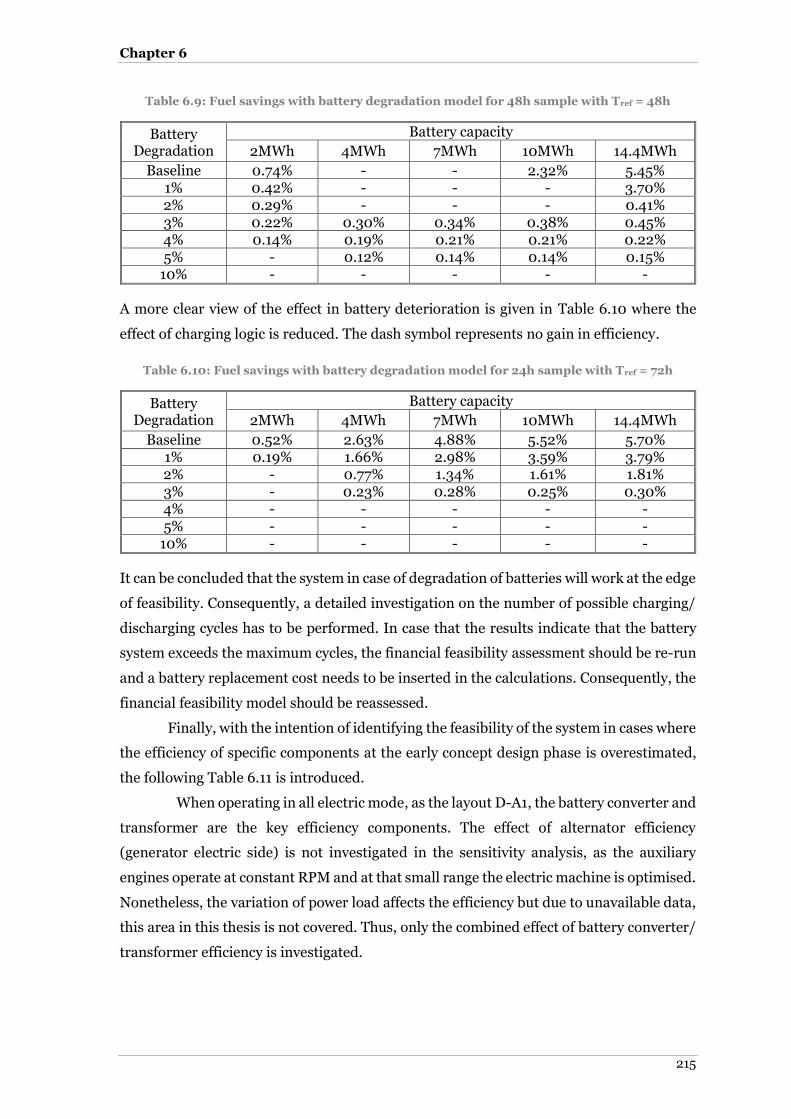
Chapter 6
215
Table 6.9: Fuel savings with battery degradation model for 48h sample with Tref = 48h
Battery Degradation
Battery capacity
2MWh 4MWh 7MWh 10MWh 14.4MWh
Baseline 0.74% - - 2.32% 5.45% 1% 0.42% - - - 3.70% 2% 0.29% - - - 0.41% 3% 0.22% 0.30% 0.34% 0.38% 0.45% 4% 0.14% 0.19% 0.21% 0.21% 0.22% 5% - 0.12% 0.14% 0.14% 0.15%
10% - - - - -
A more clear view of the effect in battery deterioration is given in Table 6.10 where the
effect of charging logic is reduced. The dash symbol represents no gain in efficiency.
Table 6.10: Fuel savings with battery degradation model for 24h sample with Tref = 72h
Battery Degradation
Battery capacity
2MWh 4MWh 7MWh 10MWh 14.4MWh
Baseline 0.52% 2.63% 4.88% 5.52% 5.70% 1% 0.19% 1.66% 2.98% 3.59% 3.79% 2% - 0.77% 1.34% 1.61% 1.81% 3% - 0.23% 0.28% 0.25% 0.30% 4% - - - - - 5% - - - - -
10% - - - - -
It can be concluded that the system in case of degradation of batteries will work at the edge
of feasibility. Consequently, a detailed investigation on the number of possible charging/
discharging cycles has to be performed. In case that the results indicate that the battery
system exceeds the maximum cycles, the financial feasibility assessment should be re-run
and a battery replacement cost needs to be inserted in the calculations. Consequently, the
financial feasibility model should be reassessed.
Finally, with the intention of identifying the feasibility of the system in cases where
the efficiency of specific components at the early concept design phase is overestimated,
the following Table 6.11 is introduced.
When operating in all electric mode, as the layout D-A1, the battery converter and
transformer are the key efficiency components. The effect of alternator efficiency
(generator electric side) is not investigated in the sensitivity analysis, as the auxiliary
engines operate at constant RPM and at that small range the electric machine is optimised.
Nonetheless, the variation of power load affects the efficiency but due to unavailable data,
this area in this thesis is not covered. Thus, only the combined effect of battery converter/
transformer efficiency is investigated.
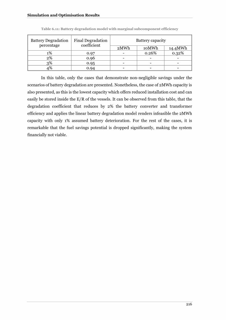
Simulation and Optimisation Results
216
Table 6.11: Battery degradation model with marginal subcomponent efficiency
Battery Degradation percentage
Final Degradation coefficient
Battery capacity
2MWh 10MWh 14.4MWh 1% 0.97 - 0.26% 0.32% 2% 0.96 - - - 3% 0.95 - - - 4% 0.94 - - -
In this table, only the cases that demonstrate non-negligible savings under the
scenarios of battery degradation are presented. Nonetheless, the case of 2MWh capacity is
also presented, as this is the lowest capacity which offers reduced installation cost and can
easily be stored inside the E/R of the vessels. It can be observed from this table, that the
degradation coefficient that reduces by 2% the battery converter and transformer
efficiency and applies the linear battery degradation model renders infeasible the 2MWh
capacity with only 1% assumed battery deterioration. For the rest of the cases, it is
remarkable that the fuel savings potential is dropped significantly, making the system
financially not viable.
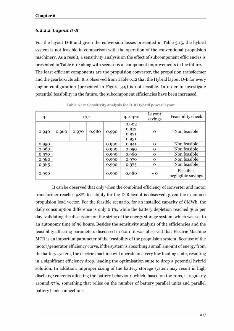
Chapter 6
217
6.2.2.2 Layout D-B
For the layout D-B and given the conversion losses presented in Table 3.15, the hybrid
system is not feasible in comparison with the operation of the conventional propulsion
machinery. As a result, a sensitivity analysis on the effect of subcomponent efficiencies is
presented in Table 6.12 along with scenarios of component improvements in the future.
The least efficient components are the propulsion converter, the propulsion transformer
and the gearbox/clutch. It is observed from Table 6.12 that the Hybrid layout D-B for every
engine configuration (presented in Figure 3.9) is not feasible. In order to investigate
potential feasibility in the future, the subcomponent efficiencies have been increased.
Table 6.12: Sensitivity analysis for D-B Hybrid power layout
ηc ηT/F ηc x ηT/F Layout savings
Feasibility check
0.940 0.960 0.970 0.980 0.990
0.902 0.912 0.921 0.931
0 Non feasible
0.950
0.990 0.941 0 Non feasible 0.960 0.990 0.950 0 Non feasible 0.970 0.990 0.960 0 Non feasible 0.980 0.990 0.970 0 Non feasible 0.985 0.990 0.975 0 Non feasible
0.990 0.990 0.980 ~ 0 Feasible,
negligible savings
It can be observed that only when the combined efficiency of converter and motor
transformer reaches 98%, feasibility for the D-B layout is observed, given the examined
propulsion load vector. For the feasible scenario, for an installed capacity of 8MWh, the
daily consumption difference is only 0.1%, while the battery depletion reached 36% per
day, validating the discussion on the sizing of the energy storage system, which was set to
an autonomy time of 96 hours. Besides the sensitivity analysis of the efficiencies and the
feasibility affecting parameters discussed in 6.2.1, it was observed that Electric Machine
MCR is an important parameter of the feasibility of the propulsion system. Because of the
motor/generator efficiency curve, if the system is absorbing a small amount of energy from
the battery system, the electric machine will operate in a very low loading state, resulting
in a significant efficiency drop, leading the optimisation suite to drop a potential hybrid
solution. In addition, improper sizing of the battery storage system may result in high
discharge currents affecting the battery behaviour, which, based on the runs, is regularly
around 97%, something that relies on the number of battery parallel units and parallel
battery bank connections.

Simulation and Optimisation Results
218
Prime movers operating at special running conditions
This section investigates the applicability of the Hybrid power layouts D-A1 and D-B in
cases where the prime mover output cannot meet the energy demand, either due to
improper design of the power system (cases of large deviation), or due to designer decision
to reduce the total installed power output, or due to emergency/ safety reasons, extra
power is required. In addition, the Hybrid power system will be assessed for cases where
over-sized engines are installed on the ship. This system is investigated under the same
conditions as those applied to the properly matched prime mover in section 6.2.1.1. In
order to investigate these special running conditions, the following statistical vector which
drops into the range of Figure 6.11 will form the input to the optimisation algorithm for
the propulsion layout (D-B-M).
11052 11052 11031 9299 7998
8876 10090 10184 7785 10335shaftP
(6.3.1)
Regarding the auxiliary layout (D-A1-M), the power profile of Figure 6.12 will form the
input to the optimisation algorithm again.
6.2.3.1 Layout D-A1-M
The first scenario to investigate is the possibility of an improper engine match with the
electric power requirements. As this has a low probability of occurence in modern ship
building, this scenario can represent cases that the electric loads are reduced during the
sea passage, in normal environmental conditions without ballast operations.
The Yanmar 6N21L engine is replaced by the MAN 6L23/30, which has an
electrical output of 730kW (characteristics were presented in Table 3.3). This engine has
significantly higher fuel efficiency, as depicted in Figure 3.8. The battery capacity is set to
2MWh which has the lowest effect in fuel savings as seen in Table 6.4 and Table 6.5. Thus
it is considered as the baseline configuration. Figure 6.16 illustrates the power split
between the up-scaled auxiliary engine and the power output of the batteries. It can be
extracted that the battery system is utilised in low generator loads only, and the system
remains idle for the 92% of the simulation time.
Consequently, the battery SoC at the final simulation step is maintained at 87.8%.
The higher fuel efficiency over a large operational range of the MAN 6L23/30 engine,
results in lower hybridisation degree of the system, when compared to the D-A1 scenario.
The effect of D-A1 in combination with this prime mover is restricted due to the steepness
of the SFOC curve of the up-scaled engine. The SFOC is flatter over a large operational
range.

Chapter 6
219
Figure 6.16: Power split between Auxiliary Engines and batteries of energy capacity 2MWh for A1 layout with up-scaled generator output
For this scenario, the auxiliary engine consumption is 1.5520 tonnes of HFO, while the
savings due to the hybrid configuration reach 0.15% of the auxiliary fuel, which is far less
than the equivalent 0.48% of the scenario where the installed energy of the battery system
was set to 2MWh.
To simulate the scenario where the designer has reduced the installed power
output of the prime movers, the Yanmar 6N21L engine is replaced by the Yanmar 6N18L,
which has an electrical output of 475kW (as seen in Table 3.3). The battery capacity is set
to 2MWh. The power split between the battery system and the auxiliary engine is presented
in Figure 6.17.
The analysis of Figure 6.17 shows that the downscaled auxiliary engine restricts
the battery usage, which is now limited to very low currents. This difference is clear when
comparing Figure 6.16 and Figure 6.17 at the 23rd and 24th simulation hours. The
downscaled layout limits the battery operation there and operates the auxiliary engine
instead. The battery peak though, around the 4th hour should be neglected. Nevertheless,
it is found that, for the given auxiliary demand profile, although the downscaled auxiliary
engine is better suited to the operational purpose, there is a slight increase of the total fuel
consumption. The consumption is now 1.58 instead of 1.55 tonnes of HFO. Nonetheless,

Simulation and Optimisation Results
220
this difference is acceptable and is explained by the higher SFOC curve that the Yanmar
engine has in comparison with the auxiliary generator set of MAN Diesel. If assuming a
downscaled engine with the same ‘parent’ SFOC curve, then the fuel consumption would
certainly be lower with the downscaled generator set. Despite this difference, the battery
system affects the fuel consumption and the reduction reaches 0.38% of the auxiliary fuel
bill.
Figure 6.17: Power split between Auxiliary Engines and batteries of energy capacity 2MWh for A1 layout with downscaled generator output
6.2.3.2 Layout D-B-M
Based on the findings of layout D-B, the hybrid system is not feasible for normal load
optimisation or high load optimisation. For this reason, the ‘parent’ engine SFOC curve for
part-load optimised engines is used. For these simulation runs, the M/E MCR is altered
according to Table 3.4. The battery energy capacity is set to 8MWh and to 10MWh. For
this optimisation scenario, the MCR of the PTO/PTI system is increased from 600kW to
1200kW and to 1800kW because the investigation involves excessive high load of the M/E
as the vessel sailed in Beaufort numbers 5 and 6 in high speed.
For this scenario, the installed MAN 7S50MC-C type engine with MCR at
11060kW is downscaled to 10500 (MCRM1) and then is replaced by the MAN 6S50MC-C
type, with a power output equal to 9800kW (MCRM2). No sensitivity analysis is performed

Chapter 6
221
for the downscale scenario. The results of the power split between the propulsion engine
and the battery system are given by Table 6.13.
Table 6.13: Power split and battery DoD for layout D-B and for downscaled M/E
Simulation segment
[-]
Simulation Time [h]
M/E load [-] Battery Power
[kW] Battery DoD [%]
MCRM1
MCRM2
MCRM1
MCRM2
MCRM1
MCRM2
1 2.4 100%
99.96% 948 1768 28% 42%
2 4.8 100% 99.96% 948 1768 57% 85% 3 7.2 100% 100% 1200 631 93% 100% 4 9.6 100% 100% 1200 1800 57% 57% 5 12 77.73% 83.28% 0 0 57% 57% 6 14.4 86.26% 100% 0 1800 57% 14% 7 16.8 100% 99.34% 1200 750 21% 32% 8 19.2 100% 97.64% 695 1050 ~0% 57% 9 21.6 74.14% 81.07% 0 0 ~0% 57% 10 24 100% 97.82% 79 1200 0% 86%
The power split indicates that there is usage of the battery system in cases (time segments
6 and 7) where the total amount of kW reserved for propulsion does not exceed the M/E
MCR, and the Hybrid controller forces the battery system to charge. This can be explained
by the shape of the part load curve, which affects the optimisation decisions, the implied
logic criteria and the equivalent future fuel saving. The implied battery charging results in
equality in fuel efficiency between the initial configuration of 11060kW and when the one
with the MCR set at 10500kW.
When the MCR is set at 9800kW there is a slight decrease in fuel efficiency by
0.10% which is negligible. Hence, it can be said that the Hybrid system is maintaining the
fuel efficiency of a properly matched engine to a configuration with downscaled prime
mover without affecting the operational capability of the vessel and without increasing the
total fuel consumption. Thus, the indirect savings occur in slow vessel speeds where the
downscaled M/E has high fuel efficiency when compared to the baseline configuration.
The Main Engine is now up-scaled and the PTO/PTI MCR is reduced to 600kW
as the M/E power is significantly increased and no large margin for the PTO/PTI system
is required. The MAN 6S70MC-C type with a power output equal to 14460kW is selected
as the propulsion engine. The batteries are fully charged prior to the application of the
shaft power profile. The high power output requirements imply the selection of high load
M/E optimisation profile. Consequently, two runs were performed, incorporating part
load optimisation for comparison with the downscale scenarios and full load optimisation
for Hybrid system assessment.
Simulation and Optimisation Results
222
The hybrid configuration over the reported period is found to be less energy
efficient and the total consumption is increased by 0.37% and for the part load
configuration the fuel consumption is increased by 0.57%. This is explained by the implied
charging current, which marginally increased the power consumption, as the total amount
of equivalent fuel savings is reduced by the existence of conversion losses, but mainly due
to the charging/discharging battery efficiency.
6.3 Chapter summary
This chapter demonstrated the accuracy of the ship simulator. The latter tool in terms of
fuel oil consumption estimation has a lower error in calculations which is around 4%
compared to the IMO formulae which result in an error of around 10%. Nonetheless, when
the ship simulator regenerates the daily parameters and the simulator has a 2 hour step
instead of a daily 24 hour step, the implied simulator error drops to 2.75%. This Chapter
also validated the fuel savings of Hybrid power system concept for Diesel Hybrid power
systems. The D-A1, D-B and D-C scenarios were investigated. For safety reasons and for
cases of improper matching of prime movers, optimisation scenarios using downscaled or
up-scaled prime movers were also performed.
Regarding the auxiliary demands, the prime mover electrical output and the
installed battery energy capacity are the controlling parameters of the hybrid power train
feasibility. Depending on the installed capacity, a hybrid system has small but non
negligible effects that can lead up to 6.19% savings of the daily auxiliary fuel consumption.
It was also demonstrated the crucial effect of the logic in charging mode which
greatly affects the fuel saving percentage. In addition, the reference time which controls
when the system is forced to have the energy storage medium charge, also contributes to
the savings percentage and hence the feasibility of the system. In addition, it was also
underlined the effect of the time step to the optimisation results and also validated the
statements of Dedes et al. (2010).
About the layout D-B, it was found that the system is infeasible. The optimisation
resulted in zero hybridization degree because of the electromechanical losses that exist
from battery towards the PTO/PTI system.
Regarding layout D-C and for part load optimised engine, although the battery
operation is restricted due to conversion losses for propulsion loads, the advanced power
management yielded to power split between the M/E and the A/E offering fuel savings that
reach 7.23% for propulsive loads. In specific loads, it was shown that this is more energy
efficient to supply power to M/E with PTI feature than use the electric machine as a shaft
generator.

Chapter 6
223
A sensitivity analysis was performed for the D-A1 and D-B scenarios. It emerged
that the hybrid system as expected is sensitive to the variation of component efficiencies.
For the layout D-B it was found that the system might run at the edge of efficiency only
when the efficiencies of the conversion and control components are close to one. Thus it
can be concluded that given the SFOC curves and the electrical and electromechnical
conversion efficiencies, the layout D-B is not feasible.
For the case of D-A1 scenario, a linear degradation battery model was applied. It
was found that the system can withstand in most of the cases a degradation of up to 2%
with potential to reach up to 4% depending on the installed battery capacity.
In the test of downscaling and up-scaling the A/E, it emerged for the up-scaled
engine that the fuel consumption is reduced primarily due to improved engine fuel
efficiency and secondly due to the application of the Hybrid solution. Regarding the
downscaled option, the system is less energy efficient due to the less efficient A/E in terms
of SFOC but still, the hybrid system offers fuel savings. Nevertheless, for the examined
power profile, the battery system operating time was reduced, as the optimisation showed
that the battery system reduces the fuel consumption in very low loads.
The same scenario was also applied to layout D-B. It was demonstrated that, for
the given power demand, a downscaled M/E along with a high output PTO/PTI system
supplied by batteries has almost negligible fuel increase due to conversion losses. The
system regularly performed a power split between the battery and the M/E, leading to the
conclusion that the system is feasible without any future component improvements. Thus,
the downscaled option leads to indirect fuel savings due to smaller engine (lower initial
cost) and due to part or low load optimisation which leads to fuel savings. Nonetheless,
the run with the up-scaled M/E showed that the system might work at the edge of its
overall efficiency and it occasionally results in temporary fuel deficiencies.

224
(Page left intentionally blank)

Chapter 7
225
7 Conclusions
This thesis investigated the potential of Hybrid Power layouts for ocean going vessels,
having as prime movers Diesel engines. The thesis applied a systematic approach to the
target areas of emission calculation, performance monitoring and energy efficiency. The
hybrid potential was based on statistical analysis of thirty-six voyages of all the modern
categories of bulkers. The analysis of the Hybrid Power system also included a concept
feasibility, constructional feasibility and financial feasibility, using statistical data sampled
by the author and structural and geometrical data of the examined ships. In order to
estimate global shipping emissions, which are quasi-static phenomena, and also to
measure the benefit of Hybrid Power systems, a time domain quasi-steady ship simulator
was constructed in a modular, scalable and extendable way.
The combination of energy storage devices for the minimisation of engine
transient loads for emissions reduction achieves fuel savings and lowers exhaust emissions
compared to conventional machinery installations. The application of this technology
involves different propulsion layouts for conventional fuel consumption. To assess over a
broad range the Hybrid Power layouts, multiple optimisation scenarios were run. A
modified version of the equivalent cost minimisation strategy was adopted and
implemented. Moreover, a pseudo multi-objective optimisation for PM and CO2 emission
reduction was also demonstrated. Savings ranging from 0.3 to 7.23% for Diesel Hybrid and
advanced energy management concept were demonstrated. In addition, a Hybrid power
system in combination with downscaled prime movers showed great potential in terms of
indirect fuel savings due to better efficiency of the prime mover. Nonetheless, the
sensitivity analysis performed for the pure Hybrid scenarios showed that the proposed
system might work at the edge of operational feasibility when the energy storage system
starts to deteriorate. The following detailed conclusions can be made:
Exhaust emission estimation
This thesis demonstrated that the adopted fuel emission factors introduce a small
percentage of uncertainty when the fuel factor corresponds to the actual burnt fuel.
Moreover, the power based factors, when divided by the engine SFOC, converge with the
correct fuel based factor. However, when an average power based factor is used, a greater
inaccuracy is introduced to the calculations. Regarding the determination of shipping
emissions, the formula of the IMO and the assumptions of the second greenhouse emission
study were compared to the results of the constructed ship simulator. It was shown that
the constructed ship simulator, using daily mean data, underestimates the shipping
emissions in the majority of the acquired sample cases; in terms of error percentage,

Conclusions
226
however, the simulator is far more accurate than the IMO study. Nevertheless, when the
simulator regenerates the environmental conditions over the 24-hour period and
recalculates the emissions over the complete voyage, the simulation results overestimate
the fuel consumption. However, the introduced error is 75% lower than the implied error,
due to the adoption of the IMO formula and of its associated assumptions.
In order to compare the cost and to determine how the hybrid system can interact
with up to date energy efficiency measures, this thesis outlined and presented all energy
saving devices and techniques. It was discussed how the proposed system is suitable for
installation alongside the majority of these measures. However, there are certain cases,
mostly in terms of energy efficiency measures targeting the propulsion machinery, which
reduce the effect of the hybrid system in certain operational profiles. Nonetheless, the
proposed system does not affect the function of these technologies, as the system is capable
of being idle when not required. Thus, the hybrid system proved to be an additional energy
saving technology, which is compatible with the latest technologies and also increases the
overall fuel saving percentage when operated.
Simulator model assessment
For the requirements of the ship simulator, various methods for hull-fluid interaction were
implemented. Regarding the calm water resistance, the Hollenbach method proved to
converge with the model test data at the design draft, while the Holtrop-Mennen method
best fits the ballast draft calm water resistance. However, both methods converge in all
drafts for Handysize and Handymax designs. Concerning the added resistance data, three
methods were implemented. The Aertssen model proved to give modest results regarding
the added resistance due to wind and waves, and better suited the majority of the reported
data. However, there are cases where the Kwon method proved to converge with the actual
reported data.
For the wind induced loads, the Blendermann method converged with the results
of the wind resistance proposed by Isherwood. Since the Blendermann method is more up
to date, it is recommended to use this method for simulation purposes.
Statistical Hybrid Power system analysis
The proposed hypothesis was that a combination of energy storage devices for
minimisation of engine transient loads for emissions and fuel reduction is a promising
alternative to conventional installations of ship machinery. This assumption was initially
validated by the statistical analysis of twenty-six voyages of thirteen types of bulkers. The
amount of demonstrated potential savings was multiplied by the appropriate emission
factors. The likely amount of savings was projected to the world fleet, by multiplying the

Chapter 7
227
results of the sample with the category percentage of the world fleet, in order to assess the
global emission benefit by adopting the proposed machinery alternative.
The voyage statistical analysis showed that a Hybrid Power system is a flexible
and efficient propulsion system for any type of vessel having a standard mission profile,
and not only with an extensive high and low load operation. The minimisation of engine
transient loading and the use of load levelling are shown to result in fuel savings and hence
emissions reductions. The latter may be reduced further through the optimisation of
propulsion and engine components. The overall AES concept proved not to be feasible for
laden operation, as the engine fluctuation fuel savings do not compensate for the
electromechanical losses. Moreover, the hybrid AES system is more suitable in
manoeuvring operation or while sailing within ECA zones. Based on the results of the
statistical analysis, the combination of slow speed Diesel and of a hybrid PTO/PTI
(scenario D-B) system with fully integrated auxiliary power generation proved to be a
feasible alternative.
The statistical analysis concluded that the operation of the fleet greatly affects the
fuel consumption and hence the emissions. Differences were observed in similar designs
(Handysize and Handymax), which were expected to have a similar engine profile and
similar consumption: it emerged that savings were negligible for Handymax vessels,
whereas significant savings were found for Handysize. This is primarily due to chartering
commands resulting in variations in voyage speeds. A secondary reason is that the
relatively small dimensions of the ship make it suitable for a wide range of loads that
greatly affect the engine operation. To extract a more universal conclusion, a larger sample
has to be investigated, using detailed operational profiles for the voyages.
The installed power requirement is shown to be highest for the Panamax category.
On the other hand, larger ships (e.g. Capesize bulkers) operate their engines closer to the
optimum points and there is less speed variation. The installation of a large energy storage
medium is thus not necessary. Analysis of the Panamax type, being between the
HandyMax and Small Capes (also known as Post-Panamax), shows a further increase in
the energy storage demand.
From an economic point of view, and not accounting for the benefit of
environmental protection, the storage medium with Sodium Nickel-Chloride proved to be
the most feasible method, with a potentially high return on initial investment. Post-
Panamax type fuel savings demonstrated that the rate of return on the investments for
both storage media cases examined is less than three years. Other ship types indicate the
system is economically feasible over a 25-year period – with the exception of the
Handymax type– with high rates of return in most cases for the Sodium Nickel Chloride

Conclusions
228
batteries. Meanwhile, whilst other storage media are still very costly when the products
reach the market, their cost is likely to drop.
The voyage analysis showed that installing hybrid power technology on-board dry
bulk ships can lead to fuel savings of up to 1.27 million USD (at the price of 520$/tonne)
per vessel and per year, assuming that 60% of the voyage time ship sails in laden and 40%
in ballast condition. This value also depends on the ship’s dimensions, the storage medium
adopted and the demand for energy availability. The emission reduction is achieved
primarily through reducing the consumption of fuel, and further reductions could be
achieved by the optimisation of the combustion process or the operation of other engine
components. The combination of a hybrid energy storage medium and the flexibility that
it offers in the coupling with the propulsor, along with other possible improvements in
hydrodynamic ship energy efficiency should allow a notable step improvement in the
overall efficiency of the ship’s propulsion systems (estimated between 2%-10%), although
this requires further systematic design studies (Molland, et al., 2009). The re-allocation of
machinery weight and battery system is deemed feasible.
Constructional feasibility assessment
The feasibility of constructing such a hybrid system was investigated for dry bulk ships, by
considering realistic loading conditions and the trim of the vessels, together with a
description of factors to be considered in any change in weight distribution. Of the
considered battery technologies, at the early stage the potential of installing Sodium Nickel
Chloride and Redox flow cell batteries was examined. It was observed that installing
Sodium Nickel Chloride batteries closely balances the weight saving due to the reduction
in carried fuel. For other batteries, a decrease of payload is required to keep the same total
displacement. The operational characteristics of the energy storage system were presented
alongside a discussion of the appropriate compartments for their housing. It appears as
though the operating temperature in Sodium Nickel Chloride batteries is a crucial criterion
in the selection of compartments, however they are an attractive choice, since the specific
energy per m3 and the energy density per kg is high. For the second selected battery type,
namely Vanadium Redox Flow Batteries, large tanks are required to store the electrolytes
(reactants) and their energy density per kilogram and per cubic meter is significantly
lower.
It was demonstrated that the equivalent propulsion system can be installed in
current ships. Two scenarios were investigated; the first includes new-builds using the
current concept design, and the second involves an innovative ship design suitable only for
new-builds. Thus, concerning the first category, the proposed areas suitable for the
installation of energy storage devices proved to be part of the engine room and the steering

Chapter 7
229
gear room. In the cargo length, the lower stool compartments were considered. The
Sodium Nickel Chloride batteries will withstand impacts, penetration and spraying with
water. Moreover, a fire test has been performed by laboratories, which proved the
robustness and the durability of this battery type. Hence, the already successful
implementation in the marine environment, through application in modern submarines,
is validated. On the other hand, Redox flow cells do not have constraints in terms of the
operational temperature. However, the storage of reactants in different tanks raises issues
for the coating of the tanks and the pumping requires power. Moreover, the storage of
reactants creates potential issues of stability due to the presence of uncontrolled free
surfaces and issues of constructional strength due to sloshing effects inside these tanks.
Concerning the second application, the new concept design involves more radical
changes. The overall design is strictly dependent on the number of prime movers and the
installed energy capacity of the storage medium. The overall feasibility is dependent on the
operating profile of the vessel, the cargo loss, the ship’s constructional design, the age of
the vessel and, finally, the overall price of retrofitting, as any payback period of the system
is directly related to the fuel savings that may be achieved due to the installation of the
Hybrid Power system.
It was demonstrated that the percentage of cargo loss is lower than 1% for
Panamax and Post-Panamax bulk carriers, dependent on the payload weight and the
presence of ballast in the examined loading cases.
Ship Voyage simulator results
The ship simulator, which is a quasi-steady time domain simulator, offered significant aid
in identifying the power demand from the propeller, which is subject to dynamic changes
due to ship added resistance and speed alternations. Primarily, the conventional Hybrid
system, which consists of Sodium Nickel Chloride batteries and conventional Diesel
Engines or generator sets, was investigated. Three potential layouts were demonstrated.
However, because conversion losses, from electrical to mechanical and vice versa, are
significant, the latter cannot be levelled by the fuel savings since the fluctuation of engine
loading has to exceed the percentage of the loading range covered by the ‘flat’ section of
the fuel consumption curve of a conventional Diesel engine. Hence, concerning the Main
Propulsion, for the examined propulsive demand, the part load optimised engine in
combination with improved efficiencies give small but non-negligible improvements in
efficiency. Regarding the cycling over batteries, the optimisation runs validated the
preliminary sizing. The total installed energy capacity proved to be sufficient for the
examined application. Furthermore, the cycles per day do not exceed the 0.2 value, which
means that for a typical operational profile, consisting of laden and ballast voyages of

Conclusions
230
maximum 340 days per year, over the expected 25-year service margin of the vessel, the
energy storage medium will not exceed the up to date maximum reported cycles of the
Sodium Nickel Chloride tests. This reduces the risk of battery replacement under normal
conditions and thus the total cost of the system remains as presented in the financial
feasibility of the Hybrid Power system.
Optimisation algorithm results
The adopted ECMS strategy is described as rule based optimisation. Logic criteria are
imposed by the designer and the algorithm has to satisfy the constraints, the rules and find
also the optimum (for implied rules) solution. The following parameters have been noted
as of big influence on the optimisation algorithm solutions.
The reference time which controls when the system is forced to have the energy
storage medium charging, also contributes to the savings percentage and also affect the
feasibility of the system. It was also found that the effect of lambda coefficient in
combination with the rule based (logic criteria) optimisation can lead the system to
infeasible solutions. In addition, it was also underlined the effect of the time step to the
optimisation results and also validated the statements of Dedes et al. (2010).
Regarding the auxiliary demands, the prime mover electrical output and the
installed battery energy capacity are the controlling parameters of the hybrid power train
feasibility. Depending on the installed capacity, hybrid has small but non negligible effects
and can reach up to 6.19% of daily auxiliary fuel consumption.
Regarding layout D-C and for part load optimised engine, it was demonstrated
that, although the battery operation is restricted due to conversion losses, the power split
for propulsive loads is feasible. The propulsion demand is covered by the main Diesel
engine and a small percentage is supplied though the PTO/PTI system which is powered
by the auxiliary engine. In specific loads, it demonstrated savings up to 7.23% and can be
concluded that PTI system is more fuel efficient than the PTO (shaft generator) mode.
Sensitivity analysis was performed for the D-A1 where savings were observed and
to the D-B layout due to the lack of feasibility with the current technological
improvements. It emerged that the Hybrid system is too sensitive on the variation of
component efficiencies, however, it can withstand a small overall efficiency drop of 2%.
For the layout D-B it was found that the system might run at the edge of efficiency only
when the efficiencies of the conversion and control components are close to one. Thus it
can be concluded that given the SFOC curves and the electrical and electromechnical
conversion efficiencies, the layout D-B is not feasible.
Chapter 7
231
For the case of D-A1 scenario, a linear degradation battery model was applied. It
was found that the system can withstand in most of the cases a degradation of up to 2%
with potential to reach up to 4% depending on the installed capacity.
Concerning the test of downscaling and up-scaling the A/E, it emerged for the up-
scaled engine that the fuel consumption is increased.. Regarding the downscaled option,
the Hybrid power system despite the introduction of conversion losses, the total
consumption in high loads (which exceed engines MCR) are almost the same than using a
normal set engine. The fuel savings occurs by optimising the engine in part and low load
configuration. Thus, hybrid couples the benefits of other fuel saving measures to
operational envelopes that before it was not possible to be applied.
The same scenario was also applied to layout D-B. The ship simulator constructed
a 24-hour voyage profile. Regarding the downscaled option, the Hybrid power system
although introduces conversion losses, the total consumption in high loads (which exceed
engines MCR) are almost the same as using a normal set engine. The fuel savings occurs
by optimising the engine in part and low load configuration. Thus, hybrid couples the
benefits of other fuel saving measures to operational envelopes that before it was not
possible to be applied. The system is feasible without any future component
improvements. Nonetheless, the run with the up-scaled M/E showed that the system
might work at the edge of its overall efficiency and it occasionally results in temporary fuel
deficiencies.
Consequently, it can be concluded that the Diesel Hybrid power train is a feasible
solution for marine application in ocean going ships with no extreme variations in engine
loading, although the results are not as remarkable as in automotive applications, where
the ICE efficiency curves are not as flat as in marine Diesel engines. Furthermore, there
are parameters that cannot be described in terms of total fuel savings, which further
improve the benefits of the Hybrid Power concept. These parameters are the operating
temperatures and pressures (e.g. NOx and PM formulation, material life cycle) and the
loading of the engine, which directly affects the external abatement technologies for
emission reduction.
The optimisation scenarios used M/E SFOC curves without having any
degradation model applied to the performance of the main engine are something that
reduces the benefit of the hybrid system. It was observed during energy audits that the
deterioration of the engine performance does not follow the curve trend of the SFOC as it
was manufactured and tuned by the engine builder. Thus, an experimental SFOC curve
should be inserted to the optimisation algorithm so as to compare directly the statistical
analysis with the results of the optimisation Thus, the differences between the statistical
analysis and the actual optimisation results rely on two major parameters. The first is the

Conclusions
232
static efficiency of the components which add uncertainty to the calculation and the second
the actual SFOC curve of each ship. Nonetheless, the statistical analysis gives a good
indication on the potential of the system in full scale application, while the optimisation
results give modest benefits as the developed algorithms compare both systems in ideal
conditions.
Novelty
This research project was the first which investigated the concept of Hybrid propulsion
and Hybrid auxiliary power train for ocean going ships consisting of battery storage system
Diesel prime movers and advanced energy management. The project modified the Hybrid
topologies proposed by the automotive industry and adapted the non-linear optimisation
procedure of the ECMS strategy for marine applications for the first time. In addition a
simple pseudo multi-objective optimisation algorithm was presented aiming at lowering
PM and NOx emissions except CO2 which remained the primary goal. The assessment of
the marine Hybrid topologies was completed by taking into account the numerous
restrictions in the application of such systems in shipping. Moreover, in the investigation
the financial and constructional feasibility has been demonstrated, something than has not
been done up to this date. Furthermore, the author had access to a number of sensitive
technical and operational information, which allowed this project to be in line with the
actual shipping business and in accordance with existing machinery and hull designs.
Nevertheless, in order to be able to increase the usage of the findings and to demonstrate
further the applicability of the proposed systems, a time domain quasi- steady simulation
tool was built. The constructed model library can assist future studies involving simulation
in this domain. Finally, the application of the simulator tool can assist shipping companies
which are aiming at higher fuel efficiency for their fleet. Currently, only few marine
consultancy companies offer Excel® based tools for performance assessment and emission
estimation with the exception of Marorka Company which develops a combination of
performance monitoring, engine control and prediction software for large maritime
companies. Therefore, the ship simulator which utilises a logical amount of computer
power can be an accurate and cheap alternative.
7.1 Discussion
‘What will be the future in marine power systems’, ‘which principles will define the modern
ship design’, ‘will the current market define the ship design for the next 25 years’? These
are some questions that arise and introduce scepticism among the ship designers. Based
on the findings of this research project, it is believed that the Hybrid power train will
dominate the ship industry in the future. Probably the first attempt will be the installation
Chapter 7
233
of multiple prime movers coupled to clutches rotating a single propeller slow speed vessel,
accepting the trade-off of increased complexity. Another potential solution is to design
slow speed twin skeg vessels which will allow a more flexible approach in engine propeller
matching. However, the flexibility, the reliability and the excessive operational profile of
the proposed Hybrid system make it applicable to future ship designs. The main advantage
of this system is that can be combined with the majority of up to date energy efficiency
measures. Moreover it can also improve the prime mover efficiency by decoupling them
from the power demand, allowing operation in more efficient points. This means that the
powering system is suitable for many purposes, something that is not dictating the
maximum or the minimum speed (a common problem of future ships which are designed
nowadays for slow steaming). A more traditional designer may say that the ships are
designed for the current market because ship-owners do not give much weight to the future
requirements as they want to maximise their current profits. This statement is clear by
taking into consideration the number of ordered and cancelled vessels and the vessel
dimensions that dominated the shipping sector. Nonetheless, this statement will not be
valid for long. Ship-owners, influenced by the global economic recession have already
identified the risks of their past choices and nowadays they pay close attention to the
requirements of flag states IMO, EU and of course the charterers including the Oil Majors.
Especially IMO takes many decisions which are not always validated by actual shipping
data, something that drives the industry in strange paths. Consequently, systems that can
serve many purposes without major retrofits and comply with future IMO regulations
should be the first choice of ship-owners willing to adapt without problems to them. In
terms of installed power, always stored energy and propulsion redundancy can decrease
the risks of collision, grounding and even total loss of the ship. To conclude, the traditional
machinery layout is likely to reach its end. Major changes of propulsion machinery in
combination with future ship designs are considered certain. Regarding the future of
Hybrid propulsion, Det Norske Veritas (DNV) had announced the installation of a Hybrid
power module on board the supply vessel ‘Viking Lady’ for assessment. This module is
consisted of an unknown type battery and a controller which will perform the energy
management. The excessive low and high needs of electrical power does not render this
case suitable for assessment of the D-B layout, however, the results will validate or not the
proposed topologies D-A1 and D-A2. Hence, the Hybrid system for Diesel powered vessels
will be judged by the shipping community in shorter time from the publication of this
thesis than initially believed, and if the statistical and simulation results are validated, then
the proposed options may become reality.

Conclusions
234
7.2 Implications for future application
There are currently no projects underway which attempt to merge specified databases of
meteorological data, ship characteristics and AIS data in order to create the appropriate
file for data loading to the simulator. As a result, by using the time domain quasi-steady
ship simulator proposed in this thesis, the fuel consumption and thus emissions can be
estimated by the application of an accurate real time bottom up approach. This tool will be
accurate enough to assess potential fuel saving device that are installed on-board,
especially if this will save historical data in a global fleet database. However, none of the
current projects for emission inventories based on AIS data can actually estimate real time
fuel consumption, as the data of ship hull and weather are available in different databases.
Regarding the ship simulator, further investigation of the models that can
describe more accurately every ship type of the examined sample is proposed. However,
this requires an extensive database of confidential data, which can only be provided by
shipping companies or by the shipyards. In addition, a detailed RAO of added resistance
versus significant wave height and wave direction would be an interesting contribution to
the ship simulator library. In addition, a dynamic approach should also be considered, but
not for emission calculation as these phenomena are quasi-static.
Concerning the optimisation suite, it is proposed to refine and improve the logic
criteria and re-run simulation cases. It would be of great interest if future comparisons
between the results of the ECMS strategy and the results of a DP were made.
Finally, the dynamic coupling in a laboratory environment of the PTO/PTI system
in fluctuating power profile with a Diesel engine requires further testing. In addition, a
dynamic controller for this purpose has to be designed and implemented. It is
recommended to perform laboratory tests, adding to the previous laboratory layout a
Sodium Nickel Chloride battery pack, so as to validate the simulated battery efficiency
curves. The latter efficiencies were obtained from experimental data, but not for marine
application and not in such a large energy capacity.

References
235
References
G. H. Abd-Alla. Using exhaust gas recirculation in internal combustion engines: a review.
Energy Conversion and Management, 43(8):1027–1042, 2002. ISSN 0196-8904.
T. Abram. Reactor thermal Hydraulics - lecture notes SESG6026, University of
Southampton MSc. The University of Manchester, Dalton Institute, 2011.
A. K. Adnanes and Norges teknisk-naturvitenskapelige universitet Institutt for marin
teknikk. Maritime electrical installations and diesel electric propulsion. Citeseer, 2003.
G. Aertssen. Service Performance and Seakeeping Trials on MV Lukuga. Trans. RINA,
page 293, 1963.
G. Aertssen. Service Performance and Seakeeping Trials on MV Jordaens. Trans., RINA,
108(4), 1966.
G. Aertssen. Service-Performance and Sea Keeping Trials on a Stern Trawler.
Transactions of the North-east coast institution of engineers and shipbuilders, page 13,
1967.
G. Aertssen. Service Performance and Trials at Sea. In 12th International Towing Tank
Conference,1969.
G. Aertssen and M. F. Sluys. Service Performance and Seakeeping trials on a large
Containership. Trans. RINA, 114, 1972.
R. Alvarez, P. Schlienger and M. Weilenmann. Effect of hybrid system battery performance
on deter- mining CO2 emissions of hybrid electric vehicles in real-world conditions.
Energy Policy, 2010. ISSN 0301-4215.
M.D. Amiridis, T. Zhang, and R.J. Farrauto. Selective catalytic reduction of nitric oxide
by hydrocar- bons. Applied Catalysis B: Environmental, 10(1-3):203–227, 1996. ISSN
0926-3373.
H. E. Anderson. Predicting wind-driven land wild fire size and shape, United States
Ministry of Agriculture, Research Paper INT-305, 1983.
K. Andersson and H. Winnes. Environmental trade-offs in nitrogen oxide removal from
ship engine exhausts. Proceedings of the Institution of Mechanical Engineers, Part M:
Journal of Engineering for the Maritime Environment, 225(1):1, 2011. ISSN 1475-0902.

References
236
P. Andreadis, C. Chryssakis, and L. Kaiktsis. Optimization of injection characteristics in a
large marine diesel engine using evolutionary algorithms. Optimization, 1:1448, 2009.
S. Ansolabehere, J. Deutch, M. Driscoll, P.E. Gray, J.P. Holdren, P.L. Joskow, R.K. Lester
and E.J. Moniz. The future of nuclear power: an interdisciplinary MIT study, 2008.
M. E. Aughey. Ship Hull Characteristics Program. Joint Meeting of the Chesapeake &
Hampton Roads Section of the Society of Naval Architects and Marine Engineers,
September 1968.
A.P. Ault, M. J. Moore, H. Furutani and K.A. Prather. Impact of emissions from the los
angeles port region on san diego air quality during regional transport events.
Environmental science & technology, 43(10):3500–3506, 2009.
A. Azaron and F. Kianfar. Dynamic shortest path in stochastic dynamic networks: Ship
routing problem. European Journal of Operational Research, 144(1):138–156, 2003.
J. Baker. New technology and possible advances in energy storage. Energy Policy,
36(12):4368–4373, 2008. ISSN 0301-4215.
T. van Beek. Technology Guidelines for Efficient Design and Operation of Ship Propulsor.
Marine news, Wartsilla, 2004.
G. Barabino, M. Carpaneto, L. Comacchio, M. Marchesoni, and GP Novella. A new energy
storage and conversion system for boat propulsion in protected marine areas. In Clean
Electrical Power, 2009 International Conference on, pages 363–369. IEEE.
F. Barnaby and J. Kemp. Too hot to handle? the future of civil nuclear power. Executive
summary, pages 7–14, 2007.
F. Barnaby, J. Kemp and Oxford Research Group. Secure Energy?: Civil Nuclear Power,
Security and Global Warming. Oxford Research Group, 2007.
W. B. van Berlekom, P. Tragardh and A. Dellhag. Large tankers-wind coefficients and
speed loss due to wind and sea. Naval Architect, (1), 1975. ISSN 0306-0209.
W. B. van Berlekom. Wind forces on modern ship forms–effects on performance. Trans.
Of the North East Institute of Engineers and ship Builders, 97(4):123–132, 1981.
S. J. Bijlsma. On minimal-time ship routing. Staats drukkerij, 1975.
W. Blendermann. Parameter identification of wind loads on ships. Journal of Wind
Engineering and Industrial Aerodynamics, 51(3):339–351, 1994. ISSN 0167-6105.

References
237
H. Bohm and G. Gutmann. Proceedings of the 13th international Electric vehicle
symposium, Vol. II p.701, 1996.
H. Bohm and J. L. Sudworth. Extended abstracts of the Electrochemical Society, Abstract
No 138, “ZEBRA-Battery: A Viable Candidate for EV”, Vol. 94-2. The electrochem. Society,
Pennington, NJ, 1994.
N. Bose, Marine Powering Prediction and Propulsors, The society of Naval Architects and
Marine Engineers, 2008.
P. Van den Bossche, J. Matheys, and J. Van Mierlo. Battery environmental analysis.
Electric and Hybrid Vehicles: Power Sources, Models, Sustainability, Infrastructure and
the Market, page 347, 2010.
V. Brslica. Plug-in hybrids and new energy storages. In Vehicle Power and Propulsion
Conference, 2009. VPPC’09. IEEE, pages 516–523. IEEE.
B. Burger, D. Kranzer. Extreme high efficiency PV-power converters, Power Electronics
and Applications, 2009. EPE '09. 13th European Conference on , vol., no., pp.1-13, 8-10
Sept. 2009
P. Cariou. Is slow steaming a sustainable means of reducing CO2 emissions from container
shipping? Transportation Research Part D: Transport and Environment, 2011.
J. S. Carlton, Marine Propellers and Propulsion, 2nd Edition, Butterworth & Heinemann,
Oxford, 2007.
S. L. Ceccio. Friction drag reduction of external flows with bubble and gas injection,
Annual review of Fluid Mechanics 42, pp. 183-203, 2010.
F. Celik. A numerical study for the effectiveness of a wake equilising duct, Ocean
Engineering 34, pp. 2138-2145, 2007.
S.G. Chalk and J.F. Miller. Key challenges and recent progress in batteries, fuel cells, and
hydrogen storage for clean energy systems. Journal of Power Sources, 159(1):73–80,
2006. ISSN 0378-7753.
Chatzilau, K., Prousalidis, I.M., Gyparis, I.K. and Vallianatos, P., Evolution of Electric
Propulsion and overview of design in an All Electric Ship. Athens : Hellenic Chamber of
Mechanics, 2006.

References
238
C. Chryssakis, A. Frangopoulos, and L. Kaitsis. Computational Study of In-Cylinder NOx
Reduction in a Large Marine Diesel Engine Using Water Injection Strategies. In 26th
CIMAC World Congress. Bergen, Norway, June 2010. CIMAC, 2010.
J. F. Cole. Battery energy-storage systems–an emerging market for lead/acid batteries.
Journal of power sources, 53(2):239–243, 1995.
J. J. Corbett, P. S. Fischbeck and S.N. Pandis. Global nitrogen and sulfur inventories for
ocean-going ships. Journal of Geophysical Research, 104(D3):3457–3470, 1999.
J. J. Corbett and H.W. Koehler. Updated emissions from ocean shipping. J. Geophys. Res,
108(D20): 4650–64, 2003.
J. J. Corbett, J.J. Winebrake, E.H. Green, P. Kasibhatla, V. Eyring, and A. Lauer. Mortality
from ship emissions: a global assessment. Environmental science & technology,
41(24):8512–8518, 2007.
J. J. Corbett, H. Wang, and J.J. Winebrake. The effectiveness and costs of speed reductions
on emissions from international shipping. Transportation Research Part D: Transport
and Environment, 14(8): 593–598, 2009.
J. J. Corbett, D. A. Lack, J. J. Winebrake, S. Harder, J. A. Silberman and M. Gold. Arctic
shipping emissions inventories and future scenarios, Atmos. Chem. Phys., 10 9689, 2010.
Cotzias Shipping Group. S&P Monthly Report. Piraeus, June 2010.
C. Daniel and J. O. Besenhard. Handbook of Battery materials Wiley VCH, Weinheim 1999
S. B. Dalsøren, M. S. Eide, Ø. Endresen, A. Mjelde, G. Gravir, and I. S. A. Isaksen. Update
on emissions and environmental impacts from the international fleet of ships: the
contribution from major ship types and ports. Atmospheric Chemistry & Physics, 9:2171–
2194, 2009.
P. de Vos and E. Versluijs. Application of Dynamic Models during Design of a Hybrid
Diesel-Fuelled PEMFC System with Fuel Reformer. In Practical design of ships and other
floating structure symposium, 2009. PRADS’09, pages 681–689. COPPE UFRJ, 2010.
E. K. Dedes. Modular thermodynamic implementation and simulation of the closed cycle
period for a cylinder of a large marine Diesel engine. Master’s thesis, School Naval
Architecture and Marine Engineering, National Technical University of Athens, July 2009.
E. K. Dedes, D. A. Hudson, and S. R. Turnock. Design of hybrid diesel-electric energy
storage systems to maximize overall ship propulsive efficiency. In Practical design of ships
References
239
and other floating structure symposium, 2010. PRADS’10, pages 703–713. COPPE UFRJ,
2010.
E. K. Dedes, D. A. Hudson, and S. R. Turnock. Assessing the potential of hybrid energy
technology to reduce exhaust emissions from global shipping. Under Review Energy
Policy, 2012a.
E. K. Dedes, D. A. Hudson, and S. R. Turnock. Technical feasibility of Hybrid Powering
systems to reduce exhaust emissions of bulk carriers. IJME transactions of RINA, 2013a.
E. K. Dedes, S. R. Turnock, D. A Hudson, and S. Hirdaris. Possible power train concepts
for nuclear powered merchant ships. In Low Carbon shipping conference, Strathclyde
University, Glascow, 2011c.
M. St Denisand W.J. Pierson. On the motion of ships in confused seas. SNAME
Transactions 61, 280–332, 1953.
J. Deutch, E. Moniz, S. Ansolabehere, M. Driscoll, P. Gray, J. Holdren, P. Joskow, R.
Lester and N. Todreas. The future of nuclear power. an MIT Interdisciplinary Study,
http://web.mit.edu/nuclearpower, 2003.
K. C. Divya and J. Østergaard. Battery energy storage technology for power systems–An
overview. Electric Power Systems Research, 79(4):511–520, 2009. ISSN 0378-7796.
DNV. Nuclear powered ships. Technical Report 2010-0685, Det Norske Veritas DNV,
2010.
C.H. Dustmann. Advances in ZEBRA batteries. Journal of Power Sources, 127(1-2):85–
92. ISSN 0378-7753, 2004.
C. Elliott and P. Dearsley. Creating systems that work: Principles of engineering systems
for the 21st century. The Royal Academy of Engineering, 14:27, 2007.
EMEP/CORINAIR. Atmospheric emission inventory guidebook. Technical report, UN
ECE, 2002.
Ø. Endresen, E. Sørgaard, J.K. Sundet, S.B. Dalsøren, I.S.A. Isaksen, T.F. Berglen, and
G. Gravir. Emission from international sea transportation and environmental impact.
Journal of Geophysical Research, 108(D17):4560, 2003.
Ø. Endresen, E. Sørgard, H.L. Behrens, P.O. Brett and I.S.A. Isaksen. A historical
reconstruction of ships’ fuel consumption and emissions. Journal of geophysical research,
112(D12):D12301, 2007.
References
240
ENTEC UK Limited. Quantification of emissions from ships associated with ship
movements between ports in the european union. Technical report, European
Commission, 2002. DG ENV.C1.
ENTEC UK Limited. Defra UK Ship Emissions Inventory. Technical report, Department
for Food and Rural Affairs, 2010. 21897-01.
V. Eyring, H. W. Kohler, J. Van Aardenne, and A. Lauer. Emissions from international
shipping: 1. the last 50 years. Journal of Geophysical Research, 110(D17):D17305, 2005.
V. Eyring, I.S.A. Isaksen, T. Berntsen, W.J. Collins, J.J. Corbett, O. Endresen, R.G.
Grainger, J. Moldanova, H. Schlager, and D.S. Stevenson. Transport impacts on
atmosphere and climate: Shipping. Atmospheric Environment, 44(37):4735–4771, 2010.
O.M. Faltinsen, K. J. Minsaas, N. Liapis, and S.O. Skjordal. Prediction of resistance and
propulsion of a ship in a seaway. In Proc. 13th Symposium on Naval Hydrodynamics,
1980.
Fathom Consulting. Energy Efficiency. The Guide, Fathom Tech, London, 2011.
A. V. Fiacco and G. P. McCormick. Nonlinear programming: sequential unconstrained
minimization techniques, Society for industrial Mathematics 4, 1990.
A.E. Fitzgerald, C. Kingsley, and S.D. Umans. Electric machinery. Tata McGraw-Hill,
2002. ISBN 0070530394.
E. J. Foeth, Decreasing frictional resistance by air lubrication, 20th International Hiswa
Symposium in Yacht Design and Yacht Construction, Amsterdam, 2008.
G. Fontaras, P. Pistikopoulos, and Z. Samaras. Experimental evaluation of hybrid vehicle
fuel economy and pollutant emissions over real-world simulation driving cycles.
Atmospheric Environment, 42(18): 4023–4035, 2008. ISSN 1352-2310.
C.A. Fragkopoulos. Shipboard Energy Systems. Athens: National Technical University of
Athens, 2007.
E.G. Frankel, H. Chen, and National Maritime Research Center. Optimization of ship
routing. National Maritime Research Center, 1980.
A. Fratta, P. Guglielmi, G. M. Pellegrino, F. Villata. DC-AC conversion strategy optimized
for battery or fuel-cell-supplied AC motor drives. Proceedings of the 2000 IEEE
International Symposium on Industrial Electronics, vol.1, no., pp.230,235, 2000 doi:
10.1109/ISIE.2000.930518
References
241
H. Fujii and T. Takahashi. Experimental study on the resistance increase of a large full
ship in regular oblique waves. J. Soc. Nav. Archit. Japan, 137, 1975.
L. Gaines, M. Singh, Argonne National Laboratory, and United States. Dept. of Energy.
Impacts of EV Battery Production on Recycling. GPO, 1996.
R. Galloway and C. Dustmann. ZEBRA® Battery-Material Cost Availability and Recycling.
In proceeding of international electric vehicle symposium (EVS-20), Ling Beach,
Canada, pages 1-9, 2003.
W. S. Gearhart and M. W. Mc Bride. Performance assessment of propeller boss cap fin type
device, 22nd ATTC, St Johns, 1989.
J. Gerritsma and W. Beukelman. Analysis of the resistance increase in waves of a fast
cargo ship. International Shipbuilding Progress, 19(217):285–293, 1972.
S. Grammatico, A. Balluchi, E. Cosoli. A series-parallel hybrid electric powertrain for
industrial vehicles. Vehicle Power and Propulsion Conference (VPPC)’10 IEEE, pp. 1-6,
2010.
J. Gravina, J. I. R. Blake, R. A. Shenoi, S. R. Turnock, S. R. Hirdaris. Concepts for a
Modular Nuclear Powered Containership. 17th International Conference on Ships and
Shipping Research. Naples, 2012.
A. Greig and R. Bucknall. Challenges for Electric Ship Design in a Low Carbon Economy.
Marine Live Workshops, Athens 2012.
G. Grigoropoulos, T. Loukakis and A. Perakis. Seakeeping standard series for oblique seas
(A synopsis), Journal of Ocean Engineering, Vol. 27, pp. 111-126, 2001.
H. Grimmelius, P. de Vos, M. Krijgsman and E. van Deursen. Control of Hybrid Ship Drive
Systems, 2011. University of Delft.
D. Griffiths. Marine Low Speed Diesel Engines. Institute of Marine Engineers, 2006.
ISBN 1902536339.
J. Gurche (ed). Encyclopedia of Electrochemical power sources. Elsevier 4, 2009.
H. E. Guldhammer and S. A. Harvald. Ship Resistance, Effect of Form and Principal
Dimensions. Akademisk Forlag Copenhagen, 1974.
C.T. Gupta and L.C.A. Batra. Marine Engine Emissions and their Control: Present and
the Future. 2010.

References
242
L. Guzzella and A. Sciarretta, Vehicle propulsion systems. 2005, Springer.
W.J. Hall. Assessment of CO2 and priority pollutant reduction by installation of
shoreside power. Resources, Conservation and Recycling, 54(7):462–467, 2010. ISSN
0921-3449.
G. J. Haltiner, H. D. Hamilton, and G. ‘Arnason. Minimal-time ship routing. Journal of
Applied Meteorology, 1:1–7, 1962.
G.L. Hanssen and R.W. James. Optimum ship routing. Journal of Navigation,
13(03):253–272, 1960.
N. Hatziargyriou, T. Karakatsanis, M. Papadopoulos, Probabilistic load flow in distribution
systems containing dispersed wind power generation, EN: IEEE Trans. Energy
Conversion. – Vol. 8, N°1, pp. 159 – 165, 1993.
J. Heywood. Internal combustion engine fundamentals (ISE). Mcgraw-Hill, 1988.
W. Henschke. Schiffbautechnisches Handbuch. 2nd edn, Verlag Technik, Berlin, 1965.
K. Hirota, K. Matsumoto, H. Orihara and H. Yoshida. Verification of Ax-Bow Effect based
on Full Scale Measurement, Journal of the Kansai Society of Naval Architects 241, pp. 33-
40, 2004.
J. Hinnenthal. Robust pareto-optimal routing of ships utilizing ensemble weather
forecasts. In Maritime Transportation and Exploitation of Ocean and Coastal Resources:
Proceedings of the 11th International Congress of the International Maritime
Association of the Mediterranean, Lisbon, Portugal, 26-30 September 2005, volume 1,
page 1045. Taylor & Francis, 2006.
HMS-Sultan. Sustainable energy Nuclear Power - lecture notes SESG6026, University of
Southampton MSc, HMS Sultan. Nuclear Department Defence Academy, 2008.
W. Hock and K. Schittkowski. A Comparative Performance Evaluation of 27 Nonlinear
Programming Codes, Computing Vol. 30, p. 335, 1983.
W. A. Hockberger. Ship design margins-issues and impacts. Naval Engineers Journal,
88(2):157–170, 1976.
J. Holtrop, G. G. J. Mennen. An approximate power prediction method, International
Shipbuilding Progress, Vol. 29, pp. 166-170, 1981.
References
243
J. Holtrop. A statistical re-analysis of resistance and propulsion data. International
Shipbuilding Progress, 31(363):272–276, 1984. ISSN 0020-868X.
U. Hollenbach, O. Reinholz. Hydrodynamic Trends in Optimising Propulsion, SPM ‘11
International Symposium on Marine Propulsors, Hamburg, 2011.
U. Hollenbach and J. Friesch . Efficient hull forms – What can be gained. 1st Intennational
Conference on Ship Efficiency, Hamburg. 2007.
H. Hori. Feasibility of a nuclear ship at crude oil price 100 per barrel, 2008.
D. T. Hountalas, G. C. Mavropoulos, and K. B. Binder. Effect of exhaust gas recirculation
(EGR) temperature for various EGR rates on heavy duty DI diesel engine performance and
emissions. Energy, 33(2):272–283, 2008. ISSN 0360-5442.
IAEA: news centre. Retrieved May 2011, from International Atomic Energy Agency:
www.iaea.org, May, 2011.
IMO. Study of Greenhouse gas emission from ships. Technical report, Norwegian Marine
Technology Research Institute - MARINTEK, 2000. MT00 A23-038.
IMO. Second greenhouse gas emission study. Technical report, International Maritime
Organisation, 2009.
R. M. Isherwood. Wind resistance of merchant ships. RINA Supplementary Papers, 115,
1974.
ITTC. The specialist committee on unconventional propulsors, 22nd International Towing
Tank Conference, Seoul, 1999.
ITTC. Testing and Extrapolation Methods Propulsion, Performance Propulsion Test,
Propulsion Committee of 23rd ITTC. International Towing Tank Conference, Bali, 2002.
R.W. James. Application of wave forecasts to marine navigation. 1957.
A. M. Jaruchi. Analysis and modelling of energy source combinations for electric vehicles.
PhD Thesis, University of Manchester, 2010.
V. Jenkins, J. S. Carlton, and R. Smart. The nuclear propulsion of merchant ships. The
Royal Academy of Engineering, 2010.
J.M.J. Journée. Prediction of Speed and Behaviour of a Ship in a Seaway, ISP, Volume 23,
No. 265, 1976.

References
244
J.M.J. Journée and J.H.C. Meijers. Ship Routeing for Optimal Performance, Transactions
IME, February, 1980.
A. Junglewitz, Der Nabeneinfluib beim Schraubenpropeller, PhD thesis, University of
Rostock, 1996.
C. G. Justus. Winds and wind system engineering, Franklin Institute Press, Philadelphia,
PA, 1978.
M. Kashiwagi. Impact of hull design on added resistance in waves—application of the
enhanced unified theory. Proceedings of the 10th International Marine Design
Conference, Trondheim, Norway, 2009.
Y. Khersonsky, M. Islam, and K. Peterson. Challenges of connecting shipboard marine
systems to medium voltage shoreside electrical power. Industry Applications, IEEE
Transactions on, 43(3):838–844, 2007.
E. Koutroulis, D. Kolokotsa, and G. Stavrakakis. Optimal design and economic evaluation
of a battery energy storage system for the maximization of the energy generated by wind
farms in isolated electric grids. Wind Engineering, 33(1):55–81, 2009.
Y. J. Kwon. Speed loss due to added resistance in wind and waves. The Naval Architect,
March: 14–16, 2008.
N. P. Kyrtatos. Marine Diesel Engines, Design and Operation. Symmetria, 1993. ISBN
9602660023.
N. P. Kyrtatos. Marine Diesel Engines and technologies for emission reduction. In
EnergyReS Scientific Forum. EnergyReS, 2009.
D. A. Lack, et al.. Particulate emissions from commercial shipping: Chemical, physical, and
optical properties, J. Geophys. Res., 114, D00F04, doi:10.1029/2008JD011300, [printed
115(D7), 2010.
J.R. Lamarsh and A.J. Baratta. Introduction to nuclear engineering. Prentice Hall, 2001.
Young-Joo Lee, A. Khaligh, A. Emadi. Advanced Integrated Bidirectional AC/DC and
DC/DC Converter for Plug-In Hybrid Electric Vehicles. Transactions on Vehicular
Technology, IEEE, vol.58, no.8, pp.3970,3980, 2009. doi: 10.1109/TVT.2009.2028070
C. Lewis. The advanced induction motor. In Power Engineering Society Summer
Meeting, 2002 IEEE, volume 1, pages 250–253. IEEE, 2007. ISBN 0780375181.

References
245
D. Lehman. Improved Propulsion with Tuned Rudder Systems, 1st International
Conference on Ship Efficiency, Hamburg, 2007.
H. Liljenberg. Utilising pre-swirl Flow – Reducing Fuel Costs. SSPA Highlights 2, 2006.
C. Lin, J. Kang, J.W. Grizzle and H. Peng. Energy Management Strategy for a Parallel
Hybrid Electric Truck. In Proceedings of the Armerican Control Conference, 2001.
D. Linden and T. B. Reddy. Handbook of batteries 3rd Edition. McGraw-Hill Handbooks,
2002.
S. Liu, A. Papanikolaou, and G. Zaraphonitis. Prediction of added resistance of ships in
waves. Ocean Engineering, 2011.
Lloyds Maritime Information Services. Lloyd's Fairplay Ship Database, 2007.
H.K. Lo and M.R. McCord. Adaptive ship routing through stochastic ocean currents:
General formulations and empirical results. Transportation Research Part A: Policy and
Practice, 32(7):547–561, 1998.
M. S. Longuet-Higgins, On the Statistical Distribution of the Heights of Sea Waves,
Journal of Marine Research, 11(3), PP. 245-266, 1952.
P. Lorange. Shipping Company Strategies: Global Management under Turbulent
Conditions, Emerald Group Publishing Limited, 2005.
MAN Diesel. MAN BW S50MC-C7 project guide. Technical report, MAN Diesel
Copenhagen, 2007.
MAN Diesel. SFOC optimisation methods. Technical report, MAN Diesel Copenhagen,
2009a.
MAN Diesel. Emission control MAN B&W Two-stroke diesel engines. Technical report,
MAN Diesel Copenhagen, 2009b.
J.F. Manwell and J.G. McGowan. Lead acid battery storage model for hybrid energy
systems. Solar Energy, 50(5):399–405, 1993.
JF Manwell, JG McGowan, EI Baring-Gould, W. Stein, and A. Leotta. Evaluation of battery
models for wind/hybrid power system simulation. In Proceedings of EWEC, 1994.
J.F. Manwell, J.G. McGowan, U. Abdulwahid, and K. Wu. Improvements to the hybrid2
battery model. In American Wind Energy Association, Windpower 2005 Conference,
Massachusetts, 2005.

References
246
R. Manzoni, M. Metzger, and G. Crugnola. Zebra electric energy storage system: From RnD
to market. Presented at HTE hi. tech. expo–Milan, 25:28, 2008.
H.S. Marcus, J.L. Beaver. An early conceptual design and feasibility analysis of a
nuclear-powered cargo vessel. PhD thesis, Massachusetts Institute of Technology, 2009.
MARPOL. MARPOL 73/78 revised ANNEX VI, MEPC59. Technical report, Internation
Maritime Organisation, 2005.
MARPOL. MARPOL ANNEX I - oil pollution. Technical report, Internation Maritime
Organisation, 2006.
Mathworks. Building an S - Function. Mathworks Inc., 2002.
V. Matthias, I. Bewersdorff, A. Aulinger and M. Quante. The Contribution of Ship
Emissions to Air Pollution in the North Sea Regions, Env. Poll., 158 (2010) 2241, 2010.
H. Maruo. The excess resistance of a ship in rough seas. International Shipbuilding
Progress, 4(35), 1957. H. Maruo. The drift of a body floating on waves. Journal of Ship
Research, 4(3):1–10, 1960.
H. Maruo. Resistance in waves. Researches on seakeeping qualities in Japan, SNAJ,
60th Aniversary Series, 8:67–102, 1963.
J.A. McDowall. Status and outlook of the energy storage market. In Power Engineering
Society General Meeting, 2007. IEEE, pages 1–3. IEEE, 2007.
De Meyer, P., Maes, F., Volckaert, A. 2008. Emissions from international shipping in the
Belgian part of the North Sea and the Belgian seaports, Atmospheric Environment 42, p.
196, 2008.
MER. Early nuclear tankers. Marine Engineers Review, pages 27–29, March 2011.
M.R. Mohamed, S.M. Sharkh, and F.C. Walsh. Redox flow batteries for hybrid electric
vehicles: progress and challenges. In Vehicle Power and Propulsion Conference, VPPC’09.
IEEE, pages 551–557. IEEE, 2009.
A. F. Molland and S. R. Turnock. Marine Rudders and Control Surfaces: Principle, Data,
Design and Applications, Butterworth & Heinemann, Oxford, 2007.
A.F. Molland, S.R. Turnock, and D.A. Hudson. Design metrics for evaluating the
propulsive efficiency of future ships. Proceedings of the 10th International Marine Design
Conference, Trondheim (IMDC’09), Norway, 2009.

References
247
A.F. Molland, S.R. Turnock, and D.A. Hudson. Ship resistance and propulsion: practical
estimation of ship propulsive power. Cambridge University Press, 2012.
A.F. Molland. The Maritime Engineering Reference Book. Butterworth-Heinemann,
2008. ISBN 9780750689878.
R. Moody. Preliminary power predictions during the early design stages of a ship.
Masters Dissertation, Cape Technikon, South Africa, 1996.
R.F. Mulligan. A simple model for estimating newbuilding costs. Maritime Economics
andLogistics 10, 310–321, 2008.
C. Mussardo, G. Rizzoni and Y. Guezennec. A-ECMS: An adaptive algorithm for hybrid
electric vehicle energy management. European Journal of Control, 2005. Vol. 11, p.p. 509-
524.
S. Naito. Propulsive performance of ships in actual seas. Proceedings of Seventh Osaka
Colloquium on Seakeeping and Stability, Osaka, Japan, 2008.
R. Nilsen and I. Sorfonn. Hybrid power generation systems. In Power Electronics and
Applications, 2009. EPE’09. 13th European Conference on, pages 1–9. IEEE, 2009
NKK. A New Energy-saving Bow Shape at Sea. Technical Report 86, Japan, 2002.
Nocedal, J. and S. J. Wright. Numerical Optimization, Second Edition. Springer Series in
Operations Research, Springer Verlag, 2006.
N. Norbin. Statens Skeppsprovnings anstalt, Transactions of RINA, Vol.114, 1972.
M. K. Ochi, Ocean Waves: The Stochastic Approach, Cambridge University Press, 2005.
M. Ohkusu. Added resistance in waves of hull forms with blunt bow. In Proceedings of
15th Symp. On Naval Hydrodynamics, pages 135–148, 1984.
M.W.C. Oosterveld and P. Van Oossanen. Further computer-analyzed data of the
Wageningen B-screw series. Netherlands Ship Model Basin, 1975.
K. Ouchi. Research and Development of PBCF (propeller boss cap fins) to enhance
propeller efficiency, The Motor Ship 10th International Marine Propulsion Conference,
London, 1988.
K. Ouchi, M. Tamashima, T. Kawasaki, H. Koizuka. A research and development of PBCF
(propeller boss cap fins) – 2nd report: Study on propeller slipstream and actual ship
performance, Journal of Society of Naval Architects 195, Japan, 1989.
References
248
K. Ouchi, M. Tamashima, T. Kawasaki, H. Koizuka. Research and development of PBCF
(propeller boss cap fins) – Novel energy saving device to enhance propeller efficiency,
Naval Architecture and Ocean Engineering 28, Ship and Ocean Foundation, 1992.
M.J. Osborne. A resolution to the NPV-IRR debate? The Quarterly Review of Economics
and Finance, 50(2):234–239, 2010. ISSN 1062-9769.
C.P. Padhy, D. Sen, and P.K. Bhaskaran. Application of wave model for weather routing of
ships in the north indian ocean. Natural Hazards, 44(3):373–385, 2008.
N.A. Papadakis and A.N. Perakis. Deterministic minimal time vessel routing. Operations
Research, 38(3):426–438, 1990.
G. Papalambrou and NP Kyrtatos. Control Development for Smoke Reduction Through
Inlet Manifold Air Injection During Transient Loading of Marine Diesel Engines. ASME,
2009.
G. Papalambrou, N. Alexandrakis, N. P. Kyrtatos, E. Codan, I. Vlaskos, V. Pawils, and R.
Boom. Smokeless Transient Loading of Medium/High-Speed Engines Using a Controlled
Turbocharging System. In 25th CIMAC World Congress. Vienna, Austria, May 2007.
CIMAC, 2007.
A. Papanikolaou. Ship Design, Preliminary design. Symeon, 1991. ISBN 9607346378.
C.D. Parker. Lead-acid battery energy-storage systems for electricity supply networks.
Journal of Power Sources, 100(1-2):18–28, 2001.
A. Paxian, V. Eyring, W. Beer, R. Sausen and C. Wright. Present-Day and Future Global
Bottom-Up Ship Emission Inventories Including Polar Routes, Environmental Science
Technology, 44 1333, 2010.
Petromedia LTD. bunkerworld. Retrieved March 12, 2010, from
http://www.bunkerworld.com , 2010.
R.F. Pocock. Nuclear ship propulsion. 1970.
G. Politis. Ship Resistance and Propulsion. National technical University of Athens, lecture
notes, 1991.
C. Ponce de Leon, A. Fr´ıas-Ferrer, J. Gonz´alez-Garc´ıa, DA Sz´anto, and FC Walsh.
Redox flow cells for energy conversion. Journal of Power Sources, 160(1):716–732, 2006.
ISSN 0378-7753.

References
249
J. Prousalidis, S.A. Gertsos and C.A. Frangopoulos. Electric Propulsion: from infancy to
adolesence. In proceedings of IMDC 2003: 8th International Marine Design Conference,
Athens, 2003.
J. Prousalidis, IK Hatzilau, P. Michalopoulos, I. Pavlou, and D. Muthumuni. Studying ship
electric energy systems with shaft generator. In Electric Ship Technologies Symposium,
2005 IEEE, pages 156–162. IEEE, 2005. ISBN 0780392590.
J. Prousalidis, E. Styvaktakis, E. Sofras, IK Hatzilau, and D. Muthumuni. Voltage dips in
ship systems. In Electric Ship Technologies Symposium, 2007. ESTS’07. IEEE, pages
309–314. IEEE, 2007. ISBN 1424409470.
H. N. Psaraftis and C. A. Kontovas. Balancing the economic and environmental
performance of maritime transportation. Transportation Research Part D 15: 458–462,
2010.
H.N. Psaraftis and C.A. Kontovas. CO2 emissions statistics for the world commercial fleet.
WMU Journal of Maritime Affairs, 8(1):1–25, 2009.
H. N. Psaraftis and C. A. Kontovas. Ship Emissions Study. Athens: NTUA, LMT, 2008.
D. Radan. Power electronic converters for ship propulsion electric motors. Department of
Marine Technology NTNU, 2004.
R. K. Rajput. Engineering thermodynamics: A computer approach (si units version).
Jones and Barlett, 2009.
G. Rousseau, D. Sinoquet, A. Sciarretta and Y. Milhau. Design Optimisation and Optimal
Control for Hybrid Vehicles. International Conference on Engineering, 2008. EngOpt 08.
G.D. Rodriguez. Operating experience with the chino 10 mw/40 mwh battery energy
storage facility. In Energy Conversion Engineering Conference, 1989. IECEC-89.,
Proceedings of the 24th Intersociety, pages 1641–1645. IEEE, 1989.
C. J. Rydh. Environmental assessment of vanadium redox and lead-acid batteries for
stationary energy storage. Journal of Power Sources, Vol. 80, pp 21-29, 1999.
N. Salvesen. Second-order steady state forces and moments on surface ships in oblique
regular waves. In Int. Symp. On Dynamics of Marine Vehicles and Structures in Waves,
Univ. College, London, 1974.
P. Schenzle. Windschiffe im 21sten Jahrhunbert?, Jahrbuch der Schiffbautechnischen
Gesellschaft, Springer, 2010.

References
250
N. J. Schouten, M. A. Salman and N. A. Kheir. Fuzzy Logic Control for Parallel Hybrid
Vehicles. IEEE Transactions on control systems technology. Vol. 10, 2002.
R. Schulze. SVA - Nabenkappenflossen fur Schiffspropeller, Report 2218, SVA Potsdam,
1995.
H. Schneekluth. Wake equalising duct, The Naval Architect 103, April, pp. 147-150, 1986.
H. Schneekluth and V. Bertram, Design for Efficiency and Economy, Butterworth &
Heinemann, Oxford, 1998.
D. F. Shanno. On broyden-fletcher-goldfarb-shanno method, Journal of Optimization
Theory and Applications 46, pp. 87-94, 1985.
K. D. A. Shearer and W.M. Lynn. Wind Tunnel Tests on Models of Merchant Ships. Trans.
NECI, 76(Part 5): 229–260, 1960.
W. Shi, H. T. Grimmelius, D. Stapersma. Analysis of ship propulsion system behaviour and
the impact on fuel consumption, International Shipbuilding Progress, Vol. 57, 2010.
C.S.N. Shiau, C. Samaras, R. Hauffe, and J.J. Michalek. Impact of battery weight and
charging patterns on the economic and environmental benefits of plug-in hybrid vehicles.
Energy Policy, 37(7):2653–2663, 2009.
A. Shintani and R. Inoue , Influence of hull form characteristics on propulsive performance
in waves. SMWP, December, 1984.
SNAME. Marine Diesel Power Plant Practices. The Society of Naval Architects and
Marine Engineers, 1990. ISBN 960254533X.
B.K. Sovacool. Valuing the greenhouse gas emissions from nuclear power: A critical survey.
Energy Policy, 36(8):2950–2963, 2008.
LLC Starcrest consulting Group. The port of San Diego 2006 emissions inventory.
Technical report, 2008.
R. L. Steigerwald. Power electronic converter technology. Proceedings of the IEEE , vol.89,
no.6, pp.890,897, 2001 doi: 10.1109/5.931484
J. L. Sudworth. The sodium/nickel chloride (ZEBRA) battery. Journal of Power sources,
100(1-2):149–163, 2001. ISSN 0378-7753.

References
251
T. M. O’Sullivan, C. M. Bingham and R. E. Clark. Zebra Battery Technologies for the All
Electric Smart Car. International Symposium on Power Electronics. Electrical Drives,
Automation and Motion, 2006 SPEEDAM 06.
D. Sutanto and W. R. Lachs. Battery energy storage systems for sustainable energy
development in Asia. Electric power systems research, 44(1):61–67, 1998.
J. Szlapczynska and R. Smierzchalski. Adopted isochrone method improving ship safety in
weather routing with evolutionary approach. International Journal Of Reliability Quality
and Safety Engineering, 14(6): 635, 2007.
T. Tarasiuk. A few remarks about assessment methods of electric power quality on ships-
Present state and further development. Measurement, 42(8):1153–1163, 2009. ISSN
0263-2241.
R. V. Thomson and P. S. Katsoulakos. The Application of Emulsified Fuels in Diesel
Engine Designs: Experimental Results and Theoretical Predictions. Transactions of
Institute of Marine Engineers, 97, 1985.
F. R. Todd, Series 60 - Methodical Experiments with Models of Single-Screw Merchant
Ships. The David W. Taylor Model Basin, Report 1712. Washington D.C., 1963.
R. L. Townsin and YJ Kwon. Approximate formulae for the speed loss due to added
resistance in wind and waves. Tran. RINA, 125:199–207, 1983.
R. L. Townsin, B. Moss, J. B. Wynne, and IM Whyte. Monitoring the Speed Performance
of Ships. University of Newcastle, England, pages 159–177, 1975.
E. Tzannatos. Ship emissions and their externalities for the port of Piraeus-greece.
Atmospheric Environment, 44(3):400–407, 2010.
UNCTAD. Review of Maritime Transport. In United Nations Conference on Trade and
Development. United Nations, 2008.
US Army, Shore protection manual. Corps of Engineers ; Coastal Engineering Research
Center (U.S.) Volume 1, 1984.
J T. B. A. Van Kessels, Energy management for automotive power nets. Eindhoven :
Technische Universiteit Eindhoven, 2007 - Proefschrift.
A. Versluis, Computer Aided Design of Ship form by Affine Transformation. International
Shipbuilding Progress, 24 (274), 147-160, 1977.

References
252
DS Vlachos. Optimal ship routing based on wind and wave forecasts. Applied Numerical
Analysis & Computational Mathematics, 1(2):547–551, 2004.
VLCC Workgroup- F.R. Adolfen, V. Bertram, S. Collins, D. Connoly et al.. Fuel Saving
Options for VLCCs. 2009.
E. I. Vrettos and S. A. Papathanassiou. Operating policy and optimal sizing of a high
penetration RES-BESS system for small isolated grids. Energy Conversion, IEEE
Transactions on, PP(99):1 –13, 2011. ISSN 0885-8969. doi: 10.1109/TEC.2011.2129571.
R. Wagner. Large lead/acid batteries for frequency regulation, load levelling and solar
power applications. Journal of power sources, 67(1-2):163–172, 1997.
L. Wang, D.J. Lee, W.J. Lee, and Z. Chen. Analysis of a novel autonomous marine hybrid
power gener- ation/energy storage system with a high-voltage direct current link. Journal
of Power Sources, 185(2): 1284–1292, 2008.
C. Whall, D. Cooper, K. Archer, L. Twigger, N. Thurston, D. Ockwell, A. McIntyre, and A.
Ritchie. Quantification of emissions from ships associated with ship movements between
ports in the European Community. Final Report for the European Commision, Entec UK
Limited, 2002.
PA Wilson. A review of the methods of calculation of added resistance for ships in a seaway.
Journal of wind engineering and industrial aerodynamics, 20(1-3):187–199, 1985.
D. Woodyard. Pounder’s marine diesel engines and gas turbines. Butterworth-
Heinemann, 2009. ISBN 0750689846.
H. Klen Woud, D. Stapersma, Science Institute of Marine Engineering, and Technology.
Design of propulsion and electric power generation systems. IMarEST, 2003. ISBN
1902536479.
A. A. Wright. Exhaust emissions from combustion machinery. Institute of Marine
Engineers, 2000. ISBN 1902536177.
GJ Van Wylen and RE Sonntag. Fundamentals of classical thermodynamics, SI version,
744 pp. John Wiley and Sons, New York, 1978.
Liangfei Xu, Guijun Cao, Jianqiu Li, Fuyuan Yang, Languang Lu and Minggao Ouyang and
Francisco Macia Perez (Ed.). Equivalent Consumption Minimization Strategies of Series
Hybrid City Buses, Energy Management, ISBN: 978-953-307-065-0, InTech, 2010.

References
253
M. Zheng, G.T. Reader, and J.G. Hawley. Diesel engine exhaust gas recirculation–a review
on advanced and novel concepts. Energy Conversion and Management, 45(6):883–900,
2004. ISSN 0196-8904.
R. Zoppoli. Minimum-Time Routing as an N-Stage Decision Process. Institute of
Electronics, University of Genoa, Genoa, Italy, 1972.

254
(Page left intentionally blank)

Appendices
i
Appendix I
In this appendix, the calculation process for specific mathematical models is presented. In
addition, mathematical models which were implemented but were not used further in this
project are also described.
Holtrop and Mennen calm water resistance calculations
The total calm water resistance using the Holtrop-Mennen method was given in Chapter 4
by equation (4.1.6). Thus, the components of resistance are given below:
The appendage resistance can be determined from equation (I.1.1)
2
20.5 1APP APP FeqR V S k C (I.1.1)
where,
SAPP : Wetted surface area of appendices [m2]
CF : Coefficient of frictional resistance of the ship according to ITTC-1957 [-]
The wave resistance RW is determined according to the Froude number (Fn). Hence, for
Fn>0.55
2
3 4 cos
17 2 5
dn nm F m F
W B wR c c c e
(I.1.2)
For Fn <0.4 the following equation is introduced:
2
1 4 cos
1 2 5
dn nm F m F
W A wR c c c e
(I.1.3)
Ci , mi, λ are coefficients determined in Holtrop and Mennen (1972) and Holtrop (1984)
For 0.4< Fn <0.55 an interpolation formula is suggested:
0.55 0.4
0.4
10 4
1.5
n W B W A
W W A
F R RR R
(I.1.4)
The additional resistance due to the presence of a bulbous bow near the surface is
determined by:

Appendices
ii
23 3 1.5
2
0.11
1
BP
ni BTB
ni
e F A gR
F
(I.1.5)
The additional pressure resistance due to the immersed transom is determined by:
2
60.5TR w TRR V A c (I.1.6)
The model-ship correlation resistance RA is given by:
20.5A w AR V S C
(I.1.7)
Hydrodynamic induced loads calculations
If the propeller is assumed as an actuator disk of known diameter and area, which is
advancing over an undisturbed fluid at speed V0, the speed at the rudder, whose leading
edge is at distance X downstream of the propeller disk, can be determined by:
1 1 2 0T A V V V (I.2.0)
VO : Undisturbed fluid speed at propeller [m/s]
V1 : accelerated speed at the propeller disk [m/s]
V2 : accelerated speed downstream of propeller disk [m/s]
By applying the Bernoulli equation and by arranging appropriately (I.2.0), it can be said
that:
2
0
1
82 TKTV
A J
(I.2.0)
The Velocity V2 can be calculated using:
2 2
2
8 TKV n D
(I.2.0)
While V1 equals to:
0 21
2
V VV
(I.2.0)

Appendices
iii
Molland and Turnock (2007) propose a Guetsche type correction to V1 to account for the
flow acceleration between the propeller and the rudder. The rudder velocity is noted as
VRR. Thus, the correction for the rudder velocity, which takes into account the distance
from the propeller, is determined by:
0.5
0.50.15
1/
R
p
K
X D
(I.2.0)
X : Distance between rudder and propeller
Finally, the rudder velocity is found using (I.2.0)
0 2
81 1 1T
RR R
KV V K
J
(I.2.0)
Miscellaneous calculations for double screw vessels
The wake, thrust deduction and relative rotation propulsion coefficients for double screw
vessels are presented here. The thrust deduction factor is approximated using the following
the expressions of Holtrop and Mennen (1981) and SSPA laboratory, which have better
accuracy versus the actual coefficients of other approximations found in the literature.
Consequently,
0.325 0.01885B
Dt C
B T
(I.3.1)
1.67 2.3 1.5BB
WP
Ct w C
C
(I.3.2)
The wake coefficient is approximated by Holtrop and Mennen (1981) and Kruger (1976),
respectively. Thus,
0.3095 10 0.23B V B
Dw C C C
B T
(I.3.3)

Appendices
iv
0.81 0.34B
w C (I.3.4)
The relative rotation efficiency is calculated by the formula proposed by Holtrop and
Mennen (1981).Therefore,
0.99737 0.111 0.0225 0.06325R P
PC lcb
D (I.3.5)
Wind Generation parameters
The wind model is a four-component model and is given by (4.8.10).The following
equations describe each subcomponent of (4.8.10).
The base wind component (VWB) is a constant number. This component is assumed to be
always present when the Beaufort number exceeds 3.
The gust wind velocity component is described by the equation:
1
cos 1 1
1
0
0
G
WG G G G
G G
t T
V V T t T T
t T T
(I.4.1)
where,
1
cos 1 cos 22
G G
G G
MX TtV
T T
(I.4.2)
The wind bust model is considered an essential component of wind velocity for dynamic
studies (Anderson et al. 1983), especially when investigating transient loads.
The ramp wind velocity component is described by the equation:
1
1 2
2
0
0
R
WG ramp R R
R
t T
V V T t T
t T
(I.4.3)
where,

Appendices
v
2
1 2
1R
ramp R
R R
t TV MX
T T
(I.4.4)
It should be noted that T2R>T1R.
The final wind velocity component is a random noise component, which is defined by:
1
2 cosN
WN V i i i
i
V s t
(I.4.5)
where,
1
2i i
(I.4.6)
Thus,
2
4/32
2
2
1
N T i
v i
T i
w
K Fs
F
u
(I.4.7)
The surface drag coefficient (KN) equals 0.004, the Turbulence scale factor (FT) equals
2000. The following parameters have been attained from empirical data but, according to
Anderson et al. (1983), they provide results of excellent accuracy when used. Thus, the
sampling rate should be equal to at least 50 and the Δω ranging from 0.5 – 2.0 rad/s.
The wind noise component equation can be replaced using a Gaussian white noise
generator. White noise has been used in sea wave modelling, offering pseudo-realistic
conditions and not smooth and/or perfect representations of the actual sea environment.

Appendices
vi
Appendix II
This appendix contains tabular data which area applicable to conventional Diesel
installation. Detailed tables of equipment located into a conventional engine room are
presented in Appendix Table 3. This information is of vital importance to assess the
constructional feasibility of the Hybrid system which is presented in Chapter 3.
Appendix Table 1: Electric Components in E/R of a modern cruise ship
No Component Installed No Volume Weight
1 Propulsion
Transformers type I 4 159.94 47200
2 Component 1 6.48 -
3 Propulsion
Converter type II
4 Component 1 2 18.30 23600
5 Component 2 2 41.47 -
6 Component 3 2 49.28 23600
7 Component 4 2 33.28 -
8 Propulsion
Converter type I
9 Component 1 1 27.66 -
10 Component 2 2 65.28 23600
11 Component 3 1 26.93 -
12 Component 4 1 16.64 -
13 Engine
Transformers type II 2 28.56 11600
14 Component 1 1 3.60 557
15 Engine
Transformers type I 3 69.12 24000
16 Component 1 1 3.60 557
17 Main Switchboards 1 104.40 3300
18 Secondary
Switchboard 1 1 35.28 684
19 Secondary
Switchboard 2 1 56.88 275
20 Motor Load Control 2 12.672 -
21 Electric Motors 2 274.56 300000
SUM: 1033.94 458.98
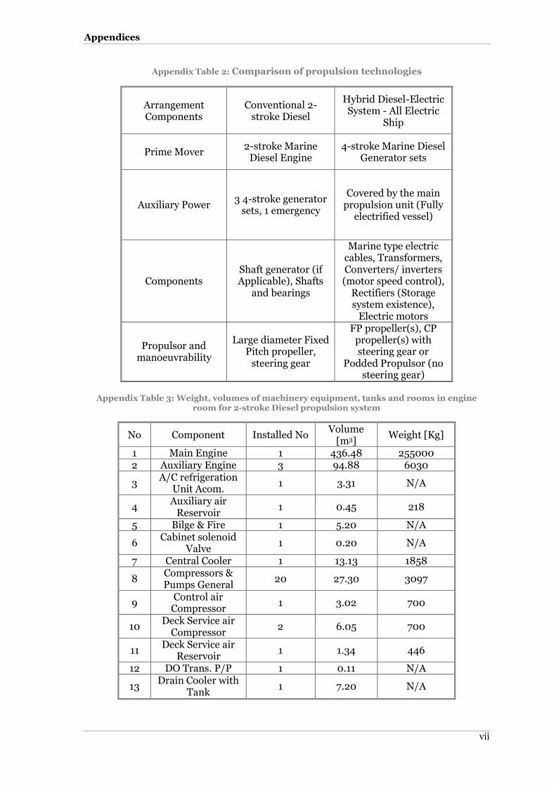
Appendices
vii
Appendix Table 2: Comparison of propulsion technologies
Arrangement Components
Conventional 2-stroke Diesel
Hybrid Diesel-Electric System - All Electric
Ship
Prime Mover 2-stroke Marine
Diesel Engine 4-stroke Marine Diesel
Generator sets
Auxiliary Power 3 4-stroke generator
sets, 1 emergency
Covered by the main propulsion unit (Fully
electrified vessel)
Components Shaft generator (if Applicable), Shafts
and bearings
Marine type electric cables, Transformers, Converters/ inverters (motor speed control),
Rectifiers (Storage system existence),
Electric motors
Propulsor and manoeuvrability
Large diameter Fixed Pitch propeller,
steering gear
FP propeller(s), CP propeller(s) with steering gear or
Podded Propulsor (no steering gear)
Appendix Table 3: Weight, volumes of machinery equipment, tanks and rooms in engine room for 2-stroke Diesel propulsion system
No Component Installed No Volume
[m3] Weight [Kg]
1 Main Engine 1 436.48 255000 2 Auxiliary Engine 3 94.88 6030
3 A/C refrigeration
Unit Acom. 1 3.31 N/A
4 Auxiliary air
Reservoir 1 0.45 218
5 Bilge & Fire 1 5.20 N/A
6 Cabinet solenoid
Valve 1 0.20 N/A
7 Central Cooler 1 13.13 1858
8 Compressors & Pumps General
20 27.30 3097
9 Control air
Compressor 1 3.02 700
10 Deck Service air
Compressor 2 6.05 700
11 Deck Service air
Reservoir 1 1.34 446
12 DO Trans. P/P 1 0.11 N/A
13 Drain Cooler with
Tank 1 7.20 N/A

Appendices
viii
14 Drink Hydrophore
Unit 1 2.04 N/A
15 Emergency air
Compressor 1 1.34 300
16 Fresh Water
Generator 1 4.38 595
17 Fresh Water
Hydrophore Unit 1 3.00 N/A
18 FWD Seal 1 0.44 N/A 19 HFO Trans. P/P 1 0.46 N/A
20 Hot water Calorifier
1 3.51 300
21 Hyd Power Pack 1 1.53 60
22 Jacket Water cooler D/G
3 0.79 N/A
23 LO Purifier 1 9.58 242
24 LO Purifier Feed
Pump 2 0.19 N/A
25 LO Trans Pump 1 0.08 38 26 Local fire P/P 1 0.45 N/A
27 M/E & G/E FO
Supply Unit 2 31.00 220
28 M/E J.W. Pre-
heater 1 0.31 200
29 M/E Jacket F.W.
Cooler 1 0.19 319
30 M/E Jacket Water
Pump 1 0.94 115
31 M/E LO Cooler 1 4.70 3820
32 Main air
Compressor 1 0.96 480
33 Main Air Reservoir
2 15.87 4530
34 Main Central CFW
P/P 3 0.94 1764
35 Main CSW P/P 1 6.00 320
36 Oily Water Separator
1 8.75 650
37 Oily Water
Separator P/P 1 0.06 65
38 Purifier 1 49.03 1410 39 Ref. Prov. Plant 1 1.57 N/A 40 Sewage System 1 10.00 N/A 41 Shaft & Bearings 1 21.68 29945 42 Composite Boiler 3.00 20000
COMPARTMENTS INSIDE E.R. 42 Control Room 1 469.46 N/A
43 Engine Room
Store 1 606.16 N/A
44 Engine Room
Workshop 1 417.30 N/A
TANKS INSIDE E.R.* 45 DO SERVICE 1 33.00 35.6 46 DO SETTLING 1 39.50 29.7

Appendices
ix
47 HFO SERVICE 1 42.30 38.7 48 HFO SETTLING 1 42.30 40.8
49 HFO STORAGE 4
P 1 254.80 245.9
50 HFO STORAGE 4
S 1 419.30 404.8
51 SLUDGE 1 12.30 Depended 52 L/S FO SERVICE 1 40.10 38.7
53 L/S FO
SETTLING 1 40.10 38.7
54 CYLINDER OIL
STORAGE 1 70.30 62
55 G/E LO
STORAGE 1 29.60 26.1
56 M/E LO
STORAGE 1 36.80 32.4
57 M/E LO
SETTLING 1 29.60 26.1
58 GRAY WATER
TANK 1 26.40 Depended
SUMMATION (items marked with * not accounted)
6301 334
Engine Room Free Volume: 2910m3

Appendices
x
Appendix III
This appendix elaborates on the statistical approximation of the energy storage
requirements using the same procedure as presented in Chapter 3.
Appendix Figure 1: Energy profile regression analysis for Handysize type
As a result, Appendix Figure 1 presents the regression analysis for the Handysize bulk
carriers, Appendix Figure 2 for the handymax type, Appendix Figure 3 for the Panamax
type and Appendix Figure 4 for the capsize bulkers. For the Post-Panamax category, the
result is presented with detailed explanation in Chapter 3.
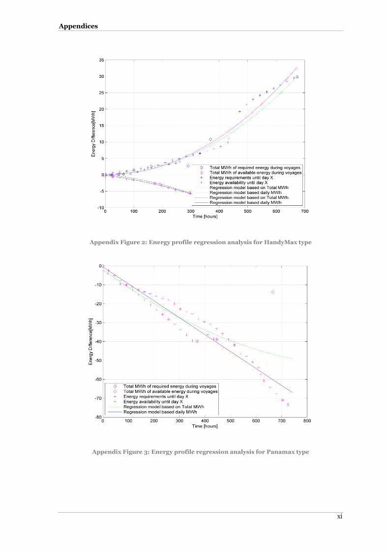
Appendices
xi
Appendix Figure 2: Energy profile regression analysis for HandyMax type
Appendix Figure 3: Energy profile regression analysis for Panamax type

Appendices
xii
Appendix Figure 4: Energy profile regression analysis for Capesize type
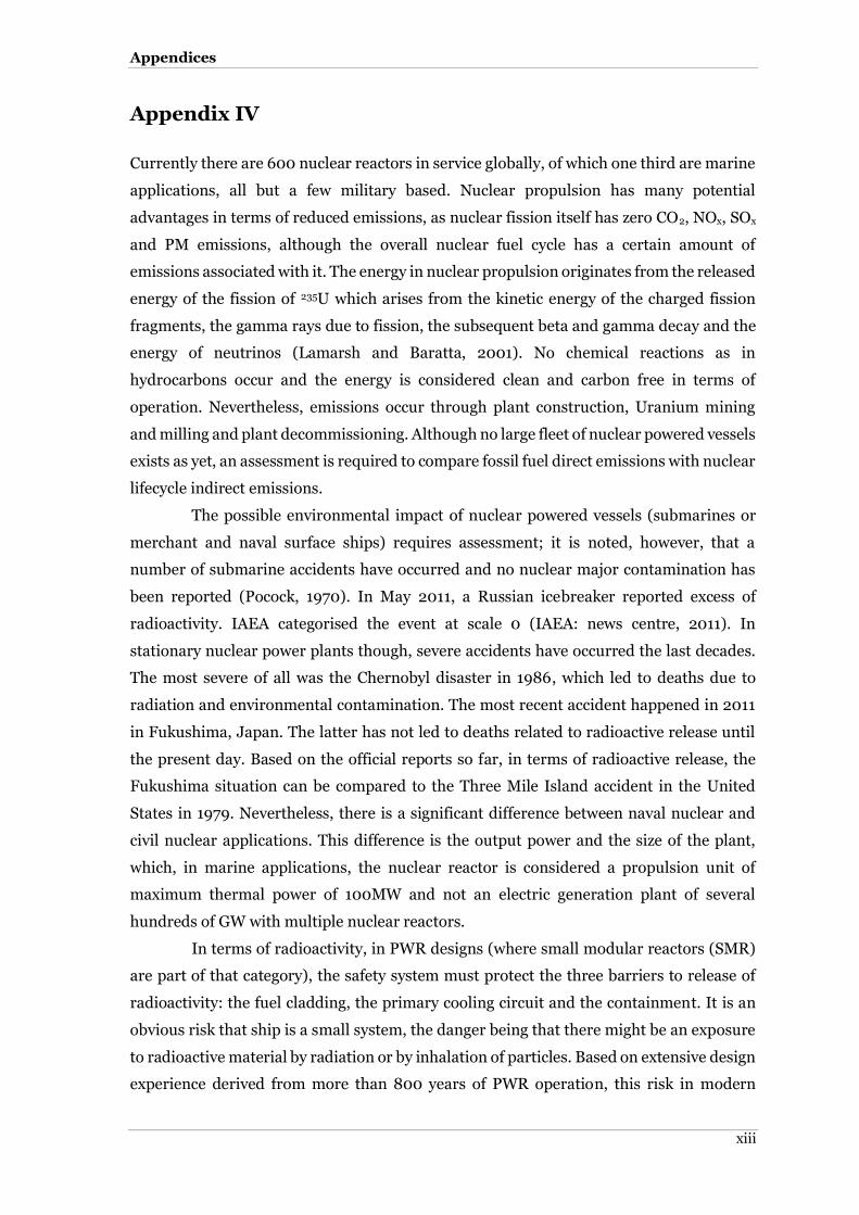
Appendices
xiii
Appendix IV
Currently there are 600 nuclear reactors in service globally, of which one third are marine
applications, all but a few military based. Nuclear propulsion has many potential
advantages in terms of reduced emissions, as nuclear fission itself has zero CO2, NOx, SOx
and PM emissions, although the overall nuclear fuel cycle has a certain amount of
emissions associated with it. The energy in nuclear propulsion originates from the released
energy of the fission of 235U which arises from the kinetic energy of the charged fission
fragments, the gamma rays due to fission, the subsequent beta and gamma decay and the
energy of neutrinos (Lamarsh and Baratta, 2001). No chemical reactions as in
hydrocarbons occur and the energy is considered clean and carbon free in terms of
operation. Nevertheless, emissions occur through plant construction, Uranium mining
and milling and plant decommissioning. Although no large fleet of nuclear powered vessels
exists as yet, an assessment is required to compare fossil fuel direct emissions with nuclear
lifecycle indirect emissions.
The possible environmental impact of nuclear powered vessels (submarines or
merchant and naval surface ships) requires assessment; it is noted, however, that a
number of submarine accidents have occurred and no nuclear major contamination has
been reported (Pocock, 1970). In May 2011, a Russian icebreaker reported excess of
radioactivity. IAEA categorised the event at scale 0 (IAEA: news centre, 2011). In
stationary nuclear power plants though, severe accidents have occurred the last decades.
The most severe of all was the Chernobyl disaster in 1986, which led to deaths due to
radiation and environmental contamination. The most recent accident happened in 2011
in Fukushima, Japan. The latter has not led to deaths related to radioactive release until
the present day. Based on the official reports so far, in terms of radioactive release, the
Fukushima situation can be compared to the Three Mile Island accident in the United
States in 1979. Nevertheless, there is a significant difference between naval nuclear and
civil nuclear applications. This difference is the output power and the size of the plant,
which, in marine applications, the nuclear reactor is considered a propulsion unit of
maximum thermal power of 100MW and not an electric generation plant of several
hundreds of GW with multiple nuclear reactors.
In terms of radioactivity, in PWR designs (where small modular reactors (SMR)
are part of that category), the safety system must protect the three barriers to release of
radioactivity: the fuel cladding, the primary cooling circuit and the containment. It is an
obvious risk that ship is a small system, the danger being that there might be an exposure
to radioactive material by radiation or by inhalation of particles. Based on extensive design
experience derived from more than 800 years of PWR operation, this risk in modern

Appendices
xiv
reactors that operate under normal conditions is considered low (DNV, 2010). In the case
of a ship, the containment compartment is shielded and protected with double bulkheads,
double bottom and double skin in case of collision and grounding. The probability of
collision to the amidships is increased compared to the stern. Unfortunately, there is a
trade-off between the risk of exposing the reactor to high accelerations and the risk of
collision and potential breach of the containment compartment.
The safe operation of ships requires the availability of propulsion power, steering
capability, navigation, and auxiliary power generation. Currently, this is mainly secured by
ensuring that each component complies with the general standards, having enhanced
reliability and performance. In nuclear powered ships, due to the high initial cost of the
reactor, it is believed that only one nuclear reactor providing enough output for the
propulsion and auxiliary loads will be installed. In case of a reactor failure, a back-up
propulsion system should be fitted, to ensure that the ship can return safely to a convenient
port and all the emergency functions can run. A combination of diesel generator and
batteries is the suitable solution. Although Diesel generators can provide enough power to
propel and provide enough electricity for cooling the decay heat of the reactor, as in land
based power plants, a second back-up system is required. Integrating the solution of
Hybrid Nuclear, batteries seem to offer both load levelling in terms of demand, and can
offer at the same time a back-up system in case of total failure. Furthermore, for a nuclear
powered ship, the energy storage coupling is also investigated for optimisation of the
secondary steam generation plant, which affects the overall efficiency of the turbo-
generators or of the propulsion turbines. The mechanical efficiency of the turbo-generators
and the turbine isentropic efficiency depends on the pressure ratio and hence the power
loading of the component (Rasjput, 2009). As a result, the objective of load levelling
practice is transformed from GHG reduction to nuclear fuel burn-up reduction in order to
increase the refuelling interval.
Regarding the safety of the nuclear reactors, the basic principles to design the
secondary safety systems are diversity (different principles of operation), redundancy
(multiple components and systems to guard against the individual failure of components),
and independence (systems have to be physically separated); they must be failsafe and
testable (tested without disrupting operation, or with redundancy). Modern reactor
designs are always under-moderated and they operate with a negative reactivity
coefficient. In case of rapid or extreme load change, turbine failure or loss of primary
coolant, the reactor will self-shut down to avoid damage. In terms of the ship accelerations
imposed on the reactor, the designer has to calculate the operational margins and match
the design with the operational profile of the ship.

Appendices
xv
In the last few decades, terrorist attacks and nuclear major accidents in Chernobyl
and Fukushima have ensured a general public awareness of the potential hazards
associated with the use of nuclear power. In shipping, another aspect arises as harbours
are usually located close to areas of large population density. Although the risk of terrorist
threat may be limited in secured ports, and the low enriched Uranium (LEU which
contains <20% of 235U) fuel is not suitable for nuclear weapons, still the political
implications and the general public opinion is believed to be against nuclear powered ships
entering the harbours. Hence, at least initially, the ship types which seem attractive are
bulk carriers and tankers. They are capable of loading /unloading away from the shore
and, as shown in , share a significant proportion of CO2 emissions. Furthermore, due to
the high initial cost which is 2.5 times the cost of conventional vessels, the HFO
consumption of these ships should be high to justify a radical change in ship design (DNV,
2010).
Implications arise concerning the operation of nuclear vessels. Firstly, not all
ports can accept these vessels. Secondly, transatlantic or transpacific voyages, during
which usually large vessels operate as liners, decrease the flexibility for chartering. Thus
nuclear powered vessels with port restrictions obstruct free economy.
Furthermore, the construction and repairs of such ships is limited to licenced
shipyards, which, again, bound the economy and potentially the construction and repair
cost would remain high due to the lack of competition.
The manning and operational costs of such vessels are still an issue. Nuclear ships
will require fully qualified and thus expensive personnel on board. The rest of the crew can
be as it is currently. However, specialised crew increases the operational cost of the vessel.
From the shipping company view, the daily performance monitoring of the fleet
and the maintenance surveying that superintendent engineers perform in dry-dockings
should change. Superintendent engineers have to attend continuing professional
development (CPD) courses in nuclear engineering so they can understand the principles
of operation and, of course, be aware of and able to identify any failures in materials caused
by radioactive exposure. Nevertheless, small modular reactors can be considered as black
boxes and might be property of the developing company, so no company engineers have
to attend such an inspection but rather, as in the early days of radio, the nuclear company
would provide the operators.

Appendices
xvi
Appendix Table 4: Global fleet (until 2007) and power trends per vessel category
Dry Bulk Carriers Number of Vessels Specified MCR up to [kW] Small and Coastal 753 2,860
Handysize 1,774 7,780 Handymax 1,732 10,600 Panamax 1,383 12,200
Post – Panamax 98 15,200 Capesize >120.000 722 18,660 and 21160 for VLBC
Total: 6,462
Container Vessels Number of Vessels Specified MCR up to [kW] Feeder – Feedermax 1,120 8,500
Handysize 1,143 21,500 Sub-Panamax 689 30,000
Panamax 568 47,000 Post-Panamax 712 78,000 New Panamax - 91,000
ULCV - 106,000 Total: 4,232
Oil Tanker Vessels Number of Vessels Specified MCR up to [kW]
Small 115 3,840 Handysize-Handymax 240 8,800 HS and 10,600 HM
Panamax 177 12,100 Aframax 648 16,000 Suezmax 332 18,700
VLCC/ ULCC >200,000dwt
516 30,000 and 44,000
Total: 2,028
The limitations that currently seem to exist in nuclear merchant shipping dictate
that a potential ship-owner has to be willing to be the first mover, to have a strong financial
position and decide that this potential is going to be a long term investment. Due to the
fact that the acceptance of a ship might be limited and hence trade restrictions might occur,
the ship-owner must be willing to accept the high risks of an unknown territory. However,
in case of success, the benefits of the prime mover can be significant.
Traditional P&I clubs cover third-party liability in case of accidents. When having
a nuclear fleet, a new trust would probably be required to cover any radiological pollution
that might occur after a serious accident. It can be said that the situation will be volatile
and a lot of steps are required before the actual operation of nuclear powered merchant
vessels can occur.
Finally, the spent fuel of global nuclear powered shipping should be considered.
PWR designs create hazardous depleted fuel. In terms of fuel economy, the worst thing to
perform is to bury the depleted fuel. The study of Deutch et al. (2003) showed that the
discovered Uranium resources are sufficient for the next 70 years, without accounting for

Appendices
xvii
the potential of nuclear shipping demand. Therefore, fuel recycling has to begin before any
nuclear renaissance. Technological improvements in fast reactor technology (Lamarsh and
Baratta, 2010) should allow the depleted fuel to be re-used, and thus the nuclear fuel cycle
can close and the actual burnt fuel can breed more, providing practically unlimited fuel for
1500 years. However, with the technology currently available, it would take almost 40-50
years to breed more fuel.
The nuclear propulsion renaissance involves a new type of nuclear reactor. The
Small Modular Reactor (SMR) and all the secondary circuits are contained into a closed to
crew box of known and small dimensions, which potentially equal the dimensions of a Fifty
feet (FEU) container. This reactor type has higher enrichment than the Pressurised Water
Reactor that is still used in naval applications. Its output is initially set to 25 MWe, which,
according to Appendix Table 5 can fit almost all categories if more than two reactors are
installed.
Because an SMR is still under design for marine applications, it can be assumed
that due to the assembly materials and their decreased volume, the associated emissions
are the lowest reported for Nuclear installations (Sovacool, 2008), a fact that makes the
nuclear potential attractive right from the beginning.
To summarise all the above, the research project aims to reduce air emissions
from global shipping using a Hybrid Power concept, which consists of high efficiency
batteries, electric generators and a slow speed Diesel engine. Although the all-electric ship
concept was investigated, efficiency issues made the solution for slow speed vessels
unattractive. The nuclear potential of a pusher barge system is also investigated in terms
of machinery sizing and efficiency. This thesis is accompanied by a ship simulator, which
incorporates multiple optimisation algorithms for calculation of savings, if any, in fuel
consumption, which are dependent on given operational scenarios.
The simulation offers an assessment tool for ship energy efficiency, of optimal
routing and of decision support for the operations department of the maritime companies.
Moreover, it is a tool for the shipping company’s technical department to control the
deterioration of the performance of their fleet. Finally, the structural and financial
feasibility of the hybrid system is demonstrated and thus the alternative system proposal
is validated in terms of most design aspects.
In the short history of nuclear power, many types of reactors have been proposed
for civil and naval applications. Power reactor systems consist primarily of five types of
reactors. The first and most commonly used category is that of light water reactors.
Pressurised water (PWR) and boiling water reactors are well-established light water
designs. The second category includes gas-cooled reactors, the third fast reactors and the
fourth evolutionary pressurised water or boiling water reactors. Recently, a fifth category

Appendices
xviii
of small modular reactors (SMR) was introduced. Modular reactors are designed by
Mitsubishi, Toshiba and Hyperion Energy. Especially for the Hyperion Energy design, the
principal characteristics are found in Appendix Table 5.
Appendix Table 5: Small Modural Reactor principal characteristics
Reactor Power: 70MWthermal
Electrical output : 25MWelectrical
Lifetime: 8 - 10 years
Size: 1.5m w by 2.5m h
Weight: Less than 50tons including pressure vessel, fuel and
primary coolant LBE
Structural material : Staineless steel
Coolant: PbBi
Fuel: Stainless clad, uranium nitride (U2N3)
Enrichment: %U-235 less than 20%
Refuel on site: No
Sealed core: Yes
License : Design certification
Passive shutdown : yes
Active Shutdown: Yes
Transportable : Yes; intact core
Factory fuelled : Yes
Safety and Control Elements: 2 redundant shutdown systems
& reactivity control rods
Not every design is feasible for marine applications, however, except PWR design
which is dominant category in naval vessels (aircraft carriers and submarines); fast
reactors are present in the navy of Russia. Currently, concept designs for vessels equipped
with SMR are underway as well. So as to have a clear picture of reactor designs, a
comparison of characteristics is made. It will be based on the several operation parameters
and on efficiency. The first and most important is the burn-up. This term describes the
energy produced per unit of mass fuel [GWdays/tonne]. A typical value of a PWR design
is 45000 GWdays/tonne compared to a gas fired boiler which is 0.4 GWdays/tonne. The
second parameter is the thermal to electrical efficiency. This efficiency comprises the
steam generator efficiency and the electric generator efficiency, which varies according to
the load. Other important parameters for the consumption of fuel are the operating
temperatures and pressures. Appendix Table 6 contains a comparison of civil reactor

Appendices
xix
designs in general. In marine applications, as previously mentioned, PWR and fast
Reactors have already been installed on naval vessels. Gas reactors, despite their high
efficiency and operating temperatures, are not viable due to their low power density.
Advanced boiling water reactor (BWR) designs should however be investigated in the
future.
Appendix Table 6: Characteristics of civil reactor commercial designs (Pocock, 1970; HMS-Sultan, 2008)
Reactor Type PWR BWR MAGNOX AGR
Fuel 3% LEU 2.2% LEU Natural
Uranium 2% LE UO2
Cladding Zircalloy Zircalloy Magnesium
alloy St. Steel
Moderator Light Water Light Water Graphite Graphite
Coolant Light Water Light Water Carbon dioxide Carbon Dioxide
Outlet Temp. 318 318 360 620
Steam Temp. 285 286 345HP 330LP
540
Steam Pressure 69 75 150 40HP 11LP
Efficiency 32% 32% 33% 42%
Power Density High High Low Low
Burn-up High High Low Low
Light water reactors consist of a pressure vessel, where the nuclear fuel, the
control rods and the moderator are present. The moderator is responsible for slowing the
fission neutrons, which increases the probability of the latter hitting another fuel atom
core and sustaining the fission. A good moderator should be cheap, should have a small
absorption cross sectional area so not to scatter the nuclei, and be chemically compatible
with the core materials. In light water reactors, the moderator also acts as a coolant.
Therefore, it should have good heat transfer capability and, over the range of operational
and fault temperatures, should have well-defined thermal properties. The main difference
between a boiling water reactor and a pressurised water reactor is the existence of a
secondary steam cycle. In PWR such a circuit exists. The steam is produced by steam
generators and the heat transfer occurs into a heat exchanger inside the reactor
compartment. The temperature at the primary circuit is on average at 325OC and the
pressure is kept at 155 bar to prevent the water from boiling, thus changing phase. Single-
phase coolant reassures the undisturbed heat exchange of the primary circuit. On the other
hand, boiling water reactors do not have a secondary steam cycle. The coolant boils and

Appendices
xx
then passes through an expander (turbine), which produces torque. No containment
structure is present as in PWR designs. Furthermore, the dangerous instabilities of the
two-phase condition of the coolant are avoided at high pressures. This means that the
design is robust. There are obvious advantages to BWR reactors. As is known, for a given
amount of water, more heat can be absorbed as latent heat (heat necessary to vaporise a
liquid) than as sensible heat, which only changes the coolant temperature. However, the
water is contaminated and the turbine should be shielded. Furthermore, the power density
of a BWR is lower than a PWR, necessitating the existence of thicker and larger pressure
vessel. Similar to the BWR concept, the RMBK type (Soviet design) utilised graphite as a
moderator and did not have a pressure vessel (Lamarsh and Baratta, 2001).
Fast reactors or Breeder Reactors differ on the principle of operation and fuel
type. Thermal reactors utilise enriched fuel and consume 238U while in operation.
However, Ansolabehere et al. (2008) state that Uranium reserves are depleting, thus
technology for recycling depleted fuel and breeder technology is investigated. A fast reactor
is found in four types: the liquid metal cooled breeder reactor (LMFBR), the gas-cooled
breeder reactor (GCFR), the molten salt breeder reactor (MSBR) and the light-water
breeder reactor (LWBR). The principle behind the operation is to fuel the reactor with
isotopes of plutonium as core, and the blanket to be natural or depleted Uranium and
breed ‘fresh’ fuel. The number of fission neutrons emitted per neutron absorbed by
Plutonium increases monotonically with increasing neutron energies above 100 keV. Thus,
no moderator is present and the effort is to sustain the velocity of neutrons. The breeder
ratio and breeding gain increase with the average energy of the neutron, including fission
in the system (Lamarsh and Baratta, 2001).
Gas cooled reactors, fed by natural Uranium and graphite moderated, were
constructed in US, UK and France for conversion of 238U to 239Pu for military purposes.
They formed the base of nuclear civil applications in nations without access to enrichment
facilities. The coolant is mainly CO2, which as a gas can operate at high temperatures,
increasing the thermal efficiency, which can reach 40%. The steam is superheated
compared to the previous mentioned designs, and their characteristics are an average
temperature of 540OC and pressure of approximately 160 bar. However, the gas has poor
heat transfer properties and requires higher surface to exchange the same amount of heat,
thus the energy density is low compared to PWR or BWR designs. Furthermore, CO2 is
susceptible to leakage, is compressible, hence it requires more pumping power and has
negligible moderating properties due to the tremendously low density (Abram, 2011).
The Small Modular Reactor (SMR) is more like a nuclear battery than a reactor
propulsion layout. It has a 36% thermal to electrical efficiency, competitive to the
European Pressurised Reactor (EPR) design of the French Areva company. These reactors

Appendices
xxi
are modular, can fit into a twenty-foot container (TEU) and weigh approximately two
tonnes per installed MWe. The fuel is LEU.
The marine environment is dynamic with continual variation in load applied to
the vessel structure with resultant motions. Unlike commercial nuclear power plants,
marine nuclear reactors must be rugged and resilient enough to withstand several decades
of rigorous operations at sea, subject to a ship's pitching and rolling and rapidly changing
demands for power, keeping the vessel speed close to that required by the operator. These
conditions, combined with the harsh environment within a reactor plant, which subjects
components and materials to the long-term effects of irradiation, corrosion, high
temperatures and pressures, necessitate an active, thorough and far-sighted technology
effort to verify reactor operation and enhance the reliability of operating plants. A nuclear
reactor is a device that should not operate under non-stable structural conditions. The
nuclear reactor should be placed near the amidships where the longitudinal centre of
buoyancy is found at design or scantling draft. The reactor compartment has to be shielded
and protected from groundings, collisions and impacts. The attractive characteristics of
the SMR reactor are that the coolant circuit operates with atmospheric pressure, thus there
is no sloshing effect caused by the vessel motions. And the reactor operation remains
undisrupted.
Unlike other shore-based electric generator plants, the marine reactor has to
operate at continuous fluctuating load. Depending on the sea state, a rise of total resistance
may lead to a power change of ~10%. Moreover, if the fluctuation of required loading
exceeds 5%, the nuclear reactor is not capable of serving the energy demand for safety
issues. If this is the case, the vessel inevitably has to reduce speed. For the peak auxiliary
loads, there is no direct problem with the nuclear operation, as they share a very small
percentage of the total installed power, hence the peak effects are negligible. Although the
rapid load change, which does not exceed 5% at a small time step, is the least important
aspect in modern nuclear reactors in respect of accident probability, because designs are
under-moderated and have always negative temperature coefficient, the operation of
turbo-machinery in non-optimum conditions increases the fuel consumption whether the
fuel is a HFO or nuclear. Despite the fact the Uranium price has been constant in the last
decades, with the exception of recent problems in mines of Canada which actually
increased the price of 238U up to four times, it is important to have fully optimised and the
least energy intensive systems from the early design stage. Minimising fuel usage will
either reduce or even completely remove the need for through life refuelling with
potentially large cost savings. Reactor technology, however, still limits the possibility for
drastic improvements in steam generation efficiency. The following graphs explain the

Appendices
xxii
Tem
pera
ture
T
em
pera
ture
steam cycles occurring in conventional and nuclear steam power plants. Appendix Figure
5 depicts a steam cycle with superheating.
Appendix Figure 5: Steam Cycle with superheating 3’-3 and one expander (turbine)
Superheating is a better way of increasing Rankine efficiency by the extra area of (3’ 3 4 4’)
(Van Wylen and Sonntag, 1978). Superheated steam ensures longer turbine life because of
the absence of erosion from high-velocity water particles that are suspended in wet vapour
(Rajput, 2009). Moreover, the Rankine cycle efficiency can be improved by increasing the
average temperature (2’ - 3’) at which heat is supplied (2- 3’), or by decreasing the
temperature at which heat is rejected (points refer to Appendix Figure 5). Appendix Figure
6 represents the actual nuclear cycle where no superheating is possible, as the cycle has to
operate at lower temperatures due to reactor constraints (Nuclear cycle typical values are:
T3’= 2850C, X3’ ~=0.9975, P3’= 69bar, while typical steam, T3=6000C, X3>1, P3= 80bar).
Appendix Figure 6: Nuclear steam cycle using two expanders, with reheating (2-3) between high pressure (HP) (1-2) turbine and low pressure (LP) turbine (3-4) and preheating/
compression (5-5’)
To increase efficiency and to protect the low pressure turbine from operating with
steam of dryness <0.9 (X<0.9), reheating occurs after the high pressure turbine (HP) and
1
2
2' 3'
44'
Entropy
3Working fluid
Saturation curve
High pressure
Low pressure
Vapour generator
(Oil Fired Boiler)
(QH)
Condenser
(QL)
Pump (WP) Expander
(turbine)
(WT)
.
.
.
.
1
2
3
4
5
5'
1
2 3
4
Entropy
Condenser
(QL)
Pump (WP) Expander
(turbine)
(WT)
.
.
.
.
Low pressure
Vapour Generator
(Nuclear Reactor)
(QH)
5'
5
4
3
Rejected Heat
High pressure

Appendices
xxiii
the steam efficiency increases. Thus, in order to increase the propulsive efficiency and
reduce the fuel burn up, the secondary circuit efficiency should be targeted.
If the coolant and moderator is light water (H2O), in order to keep it in a single
phase, the reactor maximum temperature should always be under 5500C. Although
operation with a two-phase coolant is possible (in BWR designs), it is very difficult to
control, therefore BWR designs have lower safety limits. Thus, operational risk increases
and other methods for Rankine efficiency increase have to be examined. It has been
observed that by increasing the secondary steam cycle boiler pressure, the cycle efficiency
tends to rise and reaches maximum value at about 166bar. Thermal efficiency of the cycle
increases if the Tmax (without superheating) is higher and by keeping the Tmin lower or equal
to the initial cycle. This means too that high temperature reactors have increased
efficiency.
The net efficiency of the Rankine cycle is given by equation (IV.1.1):
1 2 4 3
1 1 4
f fT PRankine
f
h h h hW Wn
Q h h
(IV.1.1)
Turbo-generator work can be defined by the following equation (IV.1.2):
0 p overallW m h h (IV.1.2)
The mass flow, pressure drop and efficiency of the turbine are described by manufacturer
system maps. Usually these systems are optimised for a broad range of operation and at
high loads, but in every other load their efficiency drops. Typical turbo-generator efficiency
values for example for an LNG operated LNG carrier vessel vary from 0.93 to 0.96.and
remain almost constant at high loads (Rajsput, 2009).
Taking into account the prime mover efficiencies, the Hybrid Power concept
involves a two-stroke Diesel Engine with auxiliary four stroke Diesel Generator Sets. Due
to the fact that 4-stroke Diesel Engines have reduced efficiency in low output powers, as
the basis of the optimisation scenario, a regular Diesel Generator is used. Furthermore, a
lower output generator will be used to measure the impact of low efficiency in combination
with the Hybrid system. Moreover, an oversized generator is used, which has higher
efficiency than in the initially examined cases. The same approach is followed for the main
propulsion Engines. However, it should be noted that the selection of a downscaled or up-
scaled Main Diesel engine is not a product of the optimisation algorithm.
Nuclear Hybrid Series-Parallel Propulsion

Appendices
xxiv
Hybrid nuclear propulsion combines the advantages of direct steam propulsion, the
flexibility of electrical systems in manoeuvring and while ship is at berth, and safety
features. The safe operation of the ship requires the availability of propulsion power,
steering capability, navigation, and auxiliary power generation. Currently, this is mainly
secured by ensuring that each component complies with the general standards, having
enhanced reliability and performance. In nuclear powered ships, due to the high initial
cost of the reactor, it is believed that only one nuclear reactor providing enough output for
the propulsion and auxiliary loads will be installed. In the event of a reactor failure, a back-
up propulsion system should be fitted, to ensure that the ship can return safely to a
convenient port and all the emergency functions can run. A combination of diesel
generator and batteries is a suitable solution. Although Diesel generators can provide
enough power to propel and provide enough electricity for cooling the decay heat of the
reactor, as in land based power plants, a second back-up system is required. The basic
principles for designing the secondary safety systems are diversity (different principles of
operation), redundancy (multiple components and systems to guard against the individual
failure of components), independence (systems have to be physically separated); they also
need to be failsafe and testable (tested without disrupting operation, or with redundancy).
Integrating the solution of Hybrid Nuclear, batteries seem to offer both load
levelling in terms of demand, can actually downscale the reactor installed thermal power
and can offer, at the same time, a back-up system in case of total failure. In normal
conditions the majority of the power generation comes from a nuclear reactor, which
produces steam through the steam generators attached to the secondary circuit. The main
characteristics of the steam are low quality, due to the absence of superheating, and the
existence of reheating between the HP and LP turbines at all stages of operation.
The ship will be considered to operate in four normal and one emergency modes
of operation, which define the Hybrid Nuclear scenarios. Appendix Figure 7 illustrates the
proposed Nuclear Hybrid configuration. The green line represents an alternative steam
and electric circuit, which is controlled by the optimisation algorithm described in Chapter
4. When the system operates using the alternative circuit, HP turbines are by-passed and
the excess of power demand that cannot be covered by the LP turbo-generators is boosted
by the energy storage module.
Scenario Nuclear – A (N-A):
The first scenario is identified as normal, where the main propulsion turbine provides the
power to the propulsor and a secondary turbo-generator, which utilises a part of the steam
flow, provides at sea basic loads only. No battery operation takes place.
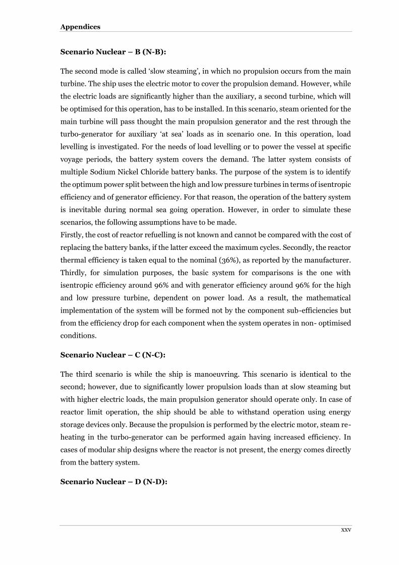
Appendices
xxv
Scenario Nuclear – B (N-B):
The second mode is called ‘slow steaming’, in which no propulsion occurs from the main
turbine. The ship uses the electric motor to cover the propulsion demand. However, while
the electric loads are significantly higher than the auxiliary, a second turbine, which will
be optimised for this operation, has to be installed. In this scenario, steam oriented for the
main turbine will pass thought the main propulsion generator and the rest through the
turbo-generator for auxiliary ‘at sea’ loads as in scenario one. In this operation, load
levelling is investigated. For the needs of load levelling or to power the vessel at specific
voyage periods, the battery system covers the demand. The latter system consists of
multiple Sodium Nickel Chloride battery banks. The purpose of the system is to identify
the optimum power split between the high and low pressure turbines in terms of isentropic
efficiency and of generator efficiency. For that reason, the operation of the battery system
is inevitable during normal sea going operation. However, in order to simulate these
scenarios, the following assumptions have to be made.
Firstly, the cost of reactor refuelling is not known and cannot be compared with the cost of
replacing the battery banks, if the latter exceed the maximum cycles. Secondly, the reactor
thermal efficiency is taken equal to the nominal (36%), as reported by the manufacturer.
Thirdly, for simulation purposes, the basic system for comparisons is the one with
isentropic efficiency around 96% and with generator efficiency around 96% for the high
and low pressure turbine, dependent on power load. As a result, the mathematical
implementation of the system will be formed not by the component sub-efficiencies but
from the efficiency drop for each component when the system operates in non- optimised
conditions.
Scenario Nuclear – C (N-C):
The third scenario is while the ship is manoeuvring. This scenario is identical to the
second; however, due to significantly lower propulsion loads than at slow steaming but
with higher electric loads, the main propulsion generator should operate only. In case of
reactor limit operation, the ship should be able to withstand operation using energy
storage devices only. Because the propulsion is performed by the electric motor, steam re-
heating in the turbo-generator can be performed again having increased efficiency. In
cases of modular ship designs where the reactor is not present, the energy comes directly
from the battery system.
Scenario Nuclear – D (N-D):
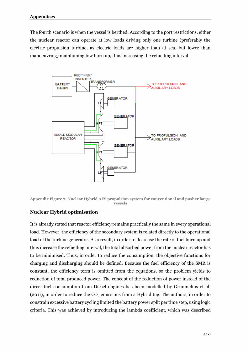
Appendices
xxvi
The fourth scenario is when the vessel is berthed. According to the port restrictions, either
the nuclear reactor can operate at low loads driving only one turbine (preferably the
electric propulsion turbine, as electric loads are higher than at sea, but lower than
manoeuvring) maintaining low burn up, thus increasing the refuelling interval.
Appendix Figure 7: Nuclear Hybrid AES propulsion system for conventional and pusher barge vessels
Nuclear Hybrid optimisation
It is already stated that reactor efficiency remains practically the same in every operational
load. However, the efficiency of the secondary system is related directly to the operational
load of the turbine generator. As a result, in order to decrease the rate of fuel burn up and
thus increase the refuelling interval, the total absorbed power from the nuclear reactor has
to be minimised. Thus, in order to reduce the consumption, the objective functions for
charging and discharging should be defined. Because the fuel efficiency of the SMR is
constant, the efficiency term is omitted from the equations, so the problem yields to
reduction of total produced power. The concept of the reduction of power instead of the
direct fuel consumption from Diesel engines has been modelled by Grimmelius et al.
(2011), in order to reduce the CO2 emissions from a Hybrid tug. The authors, in order to
constrain excessive battery cycling limited the battery power split per time step, using logic
criteria. This was achieved by introducing the lambda coefficient, which was described
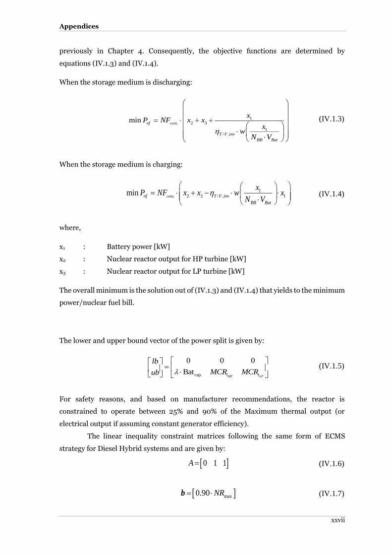
Appendices
xxvii
previously in Chapter 4. Consequently, the objective functions are determined by
equations (IV.1.3) and (IV.1.4).
When the storage medium is discharging:
.
12 3
1/ ,
minconsnf
T F inv
BB Bat
xP NF x x
xw
N V
(IV.1.3)
When the storage medium is charging:
.
12 3 / , 1min
consnf T F inv
BB Bat
xP NF x x w x
N V
(IV.1.4)
where,
x1 : Battery power [kW]
x2 : Nuclear reactor output for HP turbine [kW]
x3 : Nuclear reactor output for LP turbine [kW]
The overall minimum is the solution out of (IV.1.3) and (IV.1.4) that yields to the minimum
power/nuclear fuel bill.
The lower and upper bound vector of the power split is given by:
cap.
0 0 0
BatHP LPt t
lb
MCR MCRub
(IV.1.5)
For safety reasons, and based on manufacturer recommendations, the reactor is
constrained to operate between 25% and 90% of the Maximum thermal output (or
electrical output if assuming constant generator efficiency).
The linear inequality constraint matrices following the same form of ECMS
strategy for Diesel Hybrid systems and are given by:
0 1 1A (IV.1.6)
max0.90 NR b (IV.1.7)

Appendices
xxviii
The non-linear constraint when the storage medium is discharging is determined by:
.
2 2 2 3 3 3
/
1/ , 1
shaft aux
m is m is
C T F loss
T F inv
BB Bat
P Px x x x x x
xw x
N V
(IV.1.8)
The non-linear constraint when the storage medium is charging is determined by:
.
2 2 2 3 3 3
/
1/ , 1
shaft aux
m is m is
C T F loss
T F inv
BB Bat
P Px x x x x x
xw x
N V
(IV.1.9)
The lower and upper bound vector of the power split in charging condition is given by:
cap.
cap.
Bat 0 0
BatHP LPin t t
lb
DoD MCR MCRub
(IV.1.10)
The linear constraints that are applicable to the optimisation vector X for the charging
condition are expressed by matrices (IV.1.6) and (IV.1.7). The initial vector x0, which
enables the system to converge to the minimum solution more rapidly, is given by:
cap.
AES0 0
cap.
/ ,
Bat
1 0Bat 2
sim
T F inv
sim
t Px x
wt
(IV.1.11)
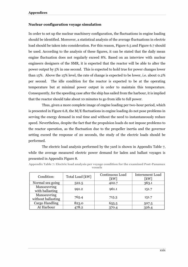
Appendices
xxix
Nuclear configuration voyage simulation
In order to set up the nuclear machinery configuration, the fluctuations in engine loading
should be identified. Moreover, a statistical analysis of the average fluctuations in electric
load should be taken into consideration. For this reason, Figure 6.5 and Figure 6.7 should
be used. According to the analysis of these figures, it can be stated that the daily mean
engine fluctuation does not regularly exceed 8%. Based on an interview with nuclear
engineers designers of the SMR, it is expected that the reactor will be able to alter the
power output by 5% in one second. This is expected to hold true for power changes lower
than 15%. Above the 15% level, the rate of change is expected to be lower, i.e. about 0.2%
per second. The idle condition for the reactor is expected to be at the operating
temperature but at minimal power output in order to maintain this temperature.
Consequently, for the speeding case after the ship has sailed from the harbour, it is implied
that the reactor should take about 10 minutes to go from idle to full power.
Thus, given a more complete image of engine loading per two-hour period, which
is presented in Figure 6.8, the M/E fluctuations in engine loading do not pose problems in
serving the energy demand in real time and without the need to instantaneously reduce
speed. Nevertheless, despite the fact that the propulsion loads do not impose problems to
the reactor operation, as the fluctuation due to the propeller inertia and the governor
setting exceed the response of 20 seconds, the study of the electric loads should be
performed.
The electric load analysis performed by the yard is shown in Appendix Table 7,
while the average measured electric power demand for laden and ballast voyages is
presented in Appendix Figure 8.
Appendix Table 7: Electric load analysis per voyage condition for the examined Post-Panamax vessels
Condition: Total Load [kW] Continuous Load
[kW] Internment Load
[kW] Normal sea going 522.5 402.7 363.1
Manoeuvring with ballasting
991.2 961.1 151.7
Manoeuvring without ballasting
765.4 715.3 151.7
Cargo Handling 823.0 655.5 507.5 At Harbour 478.2 370.4 326.4
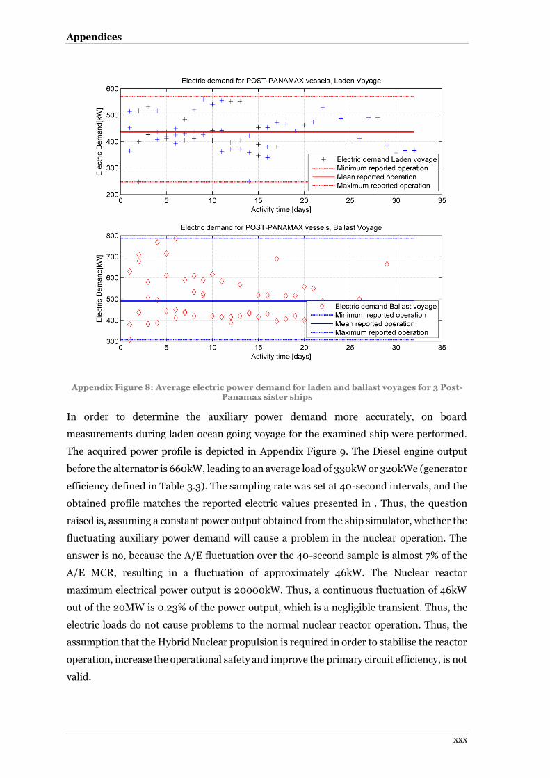
Appendices
xxx
Appendix Figure 8: Average electric power demand for laden and ballast voyages for 3 Post-Panamax sister ships
In order to determine the auxiliary power demand more accurately, on board
measurements during laden ocean going voyage for the examined ship were performed.
The acquired power profile is depicted in Appendix Figure 9. The Diesel engine output
before the alternator is 660kW, leading to an average load of 330kW or 320kWe (generator
efficiency defined in Table 3.3). The sampling rate was set at 40-second intervals, and the
obtained profile matches the reported electric values presented in . Thus, the question
raised is, assuming a constant power output obtained from the ship simulator, whether the
fluctuating auxiliary power demand will cause a problem in the nuclear operation. The
answer is no, because the A/E fluctuation over the 40-second sample is almost 7% of the
A/E MCR, resulting in a fluctuation of approximately 46kW. The Nuclear reactor
maximum electrical power output is 20000kW. Thus, a continuous fluctuation of 46kW
out of the 20MW is 0.23% of the power output, which is a negligible transient. Thus, the
electric loads do not cause problems to the normal nuclear reactor operation. Thus, the
assumption that the Hybrid Nuclear propulsion is required in order to stabilise the reactor
operation, increase the operational safety and improve the primary circuit efficiency, is not
valid.

Appendices
xxxi
Appendix Figure 9: Shipboard energy audit measurements of A/E loads
Thus, the investigation of Hybrid Nuclear propulsion will be focused only on maximising
the secondary steam circuit efficiency, which is dependent on the turbine load.
To produce a typical power profile for the main propulsion of the nuclear Hybrid
ship equipped with electric propulsion, the ship simulator will be used, but with some
modifications on the requested power from the prime mover. Due to the existence of
electric motors, power converters, propulsion transformers and transmission losses, the
following relationship should be applied:
1
shaft
demand n
component
i
PP
(IV.2.1)
The efficiencies of the electric components are presented in Table 3.2. However, in order
to simplify the propulsion problem, the efficiency of the propulsion motors will be taken
as constant and equal to 96% instead of the relationship between load and efficiency
(shown in Figure 3.7). Hence, the prime mover power, as modified for electric propulsion,
is defined by:

Appendices
xxxii
shaft shaftAES
Conventional
1 1AES
1
0.99n n
components components
i i
P PP
(IV.2.2)
To finalise the total power demand of the vessel operation, electric load which depends on
the operational scenario is added to the calculation. This average load is defined by the
electric load analysis and concerns typical ocean going operation. In order to export a
global result to the calculation, the power profile of Appendix Figure 9 will not be used in
the Nuclear Hybrid scenario.
For the baseline approximation of nuclear fuel consumption, the following assumptions
are made:
Approximately 85% of reactions leads to fission
One fission releases approximately 200MeV of energy
1 mol of U2N3 weights 518.078g
Avogadro number equals 6.02x10²³ atoms/mol
Small Modular Reactor efficiency equals to 36%
As a result, the number of fissions to meet the power demand is given by (IV.2.3):
11reactor 3.2 10
demandPA
(IV.2.3)
The number of atoms involved in the fission process is approximated by:
85%
atoms
ANo (IV.2.4)
Hence, the consumption of U2N3, which is the fuel of the examined SMR, is calculated by:
23
6
518.0786.02 10
10
atoms
N
No
FC
(IV.2.5)
The result of (IV.2.3) should be minimised using the optimisation algorithm presented in
this Appendix.

Appendices
xxxiii
Optimisation of Nuclear Hybrid installation
The assessment of the Hybrid Nuclear installation was performed on the basis of the
efficiency of the secondary circuit only. The results indicate that it is more energy efficient
to have multiple turbine sets (denoted as High Pressure or Low Pressure), instead of two
turbo generators. Thus, the following vector represents an average shaft loading. The
power demand to one motor is half of IV.3.1, as to propulsion motors cover the shaft
demand.
9300 8900 9100 7800 7200 6900AESP (IV.3.1)
To this power demand, an additional average power demand for auxiliary services was
included in the optimisation scenario. The average electric load equals to 575kW, which is
the maximum reported current, as shown in Appendix Table 7 and is higher than the
normal sea going operation. For the presented optimisation scenario, the PAES, including
the auxiliary loads, is divided by the number of electric motors, which is set to two. The
motors are connected to a gearbox with an efficiency of 98%. The HP turbo-generator
maximum output is set to 4000kW and the LP turbo-generator maximum output to
2000kW. The nuclear electric output is set to 12000kWe, with nominal thermal to
electrical efficiency of 36%. The installed battery energy capacity is set to 8000kWh and
the batteries are depleted for the optimisation scenario.
The results indicate that the proposed hybrid system with multiple turbines is
indeed less energy efficient by 3.27% than the conventional system for the given power
profile. For the propulsive and auxiliary demand of (IV.3.1), the Hybrid-Nuclear
configuration attempts to maintain the highest loads over the two turbines. This is
explained by the fact that the isentropic and motor efficiency of the HP turbine reaches its
maximum value when it operates near 100% of the load. Hence, with initially depleted
batteries and without the existence of the λ coefficient constraint, there was no need for
the system to reduce the load of turbines and utilise stored energy over the simulation
period and for the remaining simulation time, so the applied logic criterion was set
continuously to the charging condition. Nevertheless, it is stated that the logic criteria are
set in order to determine which of the Hybrid conditions (charging or discharging) yields
to the optimum global solution.
In order to evaluate the effect of the constrained optimisation, a second run is
also performed inserting the λ coefficient constraint, following exactly the same
optimisation procedure outlined in Chapter 4. Appendix Figure 10 depicts the progressive
charging of the battery during the simulated 24-hour operation. It can be extracted that

Appendices
xxxiv
the battery is now charging for 83.3% of the simulation time, until it reaches the SoCref
value, which is 35%.
The charging effect is of great importance to the percentage of power savings or
power losses. For the unconstrained system, where the battery was fully charged after two
hours of operation, power losses reached 3.71%, while, in this scenario, losses amounted
to 959.30kW or 3.27% with progressive charging. However, the results showed that the
baseline system without batteries attached is more energy efficient, as conversion losses
do not exist. In addition, these two scenarios showed that, when the battery system was
utilised and the SoC differed from SoCref, having a high propulsive power demand, the
system was more energy efficient in charging the batteries the as soon as possible, in order
to maximise energy savings. Consequently, in order to evaluate the effect of the battery
system in the Nuclear Hybrid solution, the manoeuvring condition is selected, as the
turbines work at the edge of the thermal efficiency and the turbo-generators at low loads.
The principle is to have a condition that slightly exceeds the maximum output of LP or the
HP turbine.
Appendix Figure 10: Battery Depth of Discharge in Hybrid Nuclear configuration applying λ coefficient constraint
This scenario will evaluate the need for batteries for load levelling purposes in the
Hybrid Nuclear configuration. The power demand vector for each propulsion electric

Appendices
xxxv
motor is the equal power split of the propulsion demand vector. Hence, the following
vector represents the artificial load to the LP and HP turbines. To this load, the average
auxiliary load, which equals 765kW for the ship manoeuvring without ballasting condition,
is added to the calculation. This artificial loading represents the manoeuvring of the vessel
until it reaches berth using tug assistance. The battery system is fully charged prior to this
operation.
5200 4300 3900 2800 2300 1900IAESP (IV.3.2)
Appendix Figure 11 illustrates the power split between the HP, LP and battery system. It
can be concluded from this graph that the battery system interacts and absorbs or provides
energy to the system over the examined simulation. The battery system remains idle only
for 16.7% of the simulation time. Moreover, the LP turbine is operating near its maximum
power output, increasing the energy efficiency of the system. Because the cycling over
batteries is constrained by the λ coefficient, it is impossible to meet the power demand
without running the HP turbo-generator. Thus, it is inevitable to perform a power split
between the battery and the low-pressure turbo-generator only. Nonetheless, compared to
the baseline vessel, the system is more energy demanding.
Appendix Figure 11: Power split between battery system, LP and HP turbo-generators for Nuclear Hybrid configuration
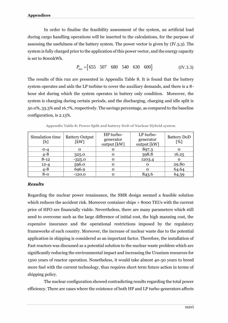
Appendices
xxxvi
In order to finalise the feasibility assessment of the system, an artificial load
during cargo handling operations will be inserted to the calculations, for the purpose of
assessing the usefulness of the battery system. The power vector is given by (IV.3.3). The
system is fully charged prior to the application of this power vector, and the energy capacity
is set to 8000kWh.
655 507 680 540 630 600auxP (IV.3.3)
The results of this run are presented in Appendix Table 8. It is found that the battery
system operates and aids the LP turbine to cover the auxiliary demands, and there is a 8-
hour slot during which the system operates in battery only condition. Moreover, the
system is charging during certain periods, and the discharging, charging and idle split is
50.0%, 33.3% and 16.7%, respectively. The savings percentage, as compared to the baseline
configuration, is 2.13%.
Appendix Table 8: Power Split and battery DoD of Nuclear Hybrid system
Simulation time [h]
Battery Output [kW]
HP turbo-generator
output [kW]
LP turbo-generator
output [kW]
Battery DoD [%]
0-4 0 0 897.3 0 4-8 325.0 0 398.8 16.25 8-12 -325.0 0 1203.4 0 12-4 596.0 0 0 29.80 4-8 696.9 0 0 64.64 8-0 -120.0 0 843.6 64.59
Results
Regarding the nuclear power renaissance, the SMR design seemed a feasible solution
which reduces the accident risk. Moreover container ships > 8000 TEUs with the current
price of HFO are financially viable. Nevertheless, there are many parameters which still
need to overcome such as the large difference of initial cost, the high manning cost, the
expensive insurance and the operational restrictions imposed by the regulatory
frameworks of each country. Moreover, the increase of nuclear waste due to the potential
application in shipping is considered as an important factor. Therefore, the installation of
Fast reactors was discussed as a potential solution to the nuclear waste problem which are
significantly reducing the environmental impact and increasing the Uranium resources for
1500 years of reactor operation. Nonetheless, it would take almost 40-50 years to breed
more fuel with the current technology, thus requires short term future action in terms of
shipping policy.
The nuclear configuration showed contradicting results regarding the total power
efficiency. There are cases where the existence of both HP and LP turbo-generators affects

Appendices
xxxvii
the overall energy efficiency, resulting in the conclusion that the system is not feasible, i.e.
in high loads. Nonetheless, it was demonstrated that, when the power demand is higher
than the maximum power output for each of turbo-generators, but less than their
combined output power, the system absorbs power from the energy storage medium,
increasing the power efficiency by up to 2.13%. However, this case is only applicable in
manoeuvring or cargo handling conditions and not in ocean going.