Air Force Institute of Technology Air Force Institute of Technology

AFIT Scholar AFIT Scholar

Theses and Dissertations Student Graduate Works

3-2020

Use of LiDAR in Automated Aerial Refueling To Improve Stereo Use of LiDAR in Automated Aerial Refueling To Improve Stereo

Vision Systems Vision Systems

Michael R. Crowl

Follow this and additional works at: https://scholar.afit.edu/etd

Part of the Computer Sciences Commons, and the Signal Processing Commons

Recommended Citation Recommended Citation Crowl, Michael R., "Use of LiDAR in Automated Aerial Refueling To Improve Stereo Vision Systems" (2020). Theses and Dissertations. 3171. https://scholar.afit.edu/etd/3171

This Thesis is brought to you for free and open access by the Student Graduate Works at AFIT Scholar. It has been accepted for inclusion in Theses and Dissertations by an authorized administrator of AFIT Scholar. For more information, please contact richard.mansfield@afit.edu.

Use of LiDAR in Automated Aerial Refueling ToImprove Stereo Vision Systems

THESIS

Michael R. Crowl, Capt, USAF

AFIT-ENG-MS-18-M-019

DEPARTMENT OF THE AIR FORCEAIR UNIVERSITY

AIR FORCE INSTITUTE OF TECHNOLOGY

Wright-Patterson Air Force Base, Ohio

DISTRIBUTION STATEMENT AAPPROVED FOR PUBLIC RELEASE; DISTRIBUTION UNLIMITED.

The views expressed in this document are those of the author and do not reflect theofficial policy or position of the United States Air Force, the United States Departmentof Defense or the United States Government. This material is declared a work of theU.S. Government and is not subject to copyright protection in the United States.

AFIT-ENG-MS-18-M-019

Use of LiDAR in Automated Aerial Refueling To Improve Stereo Vision Systems

THESIS

Presented to the Faculty

Department of Electrical and Computer Engineering

Graduate School of Engineering and Management

Air Force Institute of Technology

Air University

Air Education and Training Command

in Partial Fulfillment of the Requirements for the

Degree of Master of Science in Computer Science

Michael R. Crowl, B.S.

Capt, USAF

March 2020

DISTRIBUTION STATEMENT AAPPROVED FOR PUBLIC RELEASE; DISTRIBUTION UNLIMITED.

AFIT-ENG-MS-18-M-019

Use of LiDAR in Automated Aerial Refueling To Improve Stereo Vision Systems

THESIS

Michael R. Crowl, B.S.Capt, USAF

Committee Membership:

Scott Nykl, Ph.D.Chair

Douglas Hodson, Ph.D.Member

Clark Taylor, Ph.D.Member

AFIT-ENG-MS-18-M-019

Abstract

The United States Air Force (USAF) executes five Core Missions, four of which

depend on increased aircraft range. To better achieve global strike and reconnais-

sance, unmanned aerial vehicles (UAVs) require aerial refueling for extended missions.

However, current aerial refueling capabilities are limited to manned aircraft due to

technical difficulties to refuel UAVs mid-flight. The latency between a UAV operator

and the UAV is too large to adequately respond for such an operation. To overcome

this limitation, the USAF wants to create a capability to guide the refueling boom

into the refueling receptacle. This research explores the use of light detection and

ranging (LiDAR) to create a relative pose estimation of the UAV and compares it to

previous stereo vision results.

Researchers at the Air Force Institute of Technology (AFIT) developed an algo-

rithm to automate the refueling operation based on a stereo-vision system. While

the system works, it requires a large amount of processing; it must detect an aircraft,

compose an image between the two cameras’ points of view, create a point cloud of

the image, and run a point cloud alignment algorithm to match the point cloud to

a reference model. These complex steps require a large amount of processing power

and are subject to noise and processing artifacts.

As an alternative to stereo vision systems, AFIT will also experiment with Light

Detection and Ranging (LiDAR). A single flash LIDAR camera may perform the

same task as two stereo vision cameras and eliminate the aforementioned processing

overhead. A LIDAR will produce a point cloud model which is matched against a

reference model. Further, the point cloud a LIDAR produces will not experience the

same errors and noise artifacts as stereo vision. This may yield more accurate results

iv

compared to the stereo-vision camera system.

One more advantage to using LiDAR over stereo vision is the ability to measure

distances between the tanker and approaching aircraft. Current stereo vision research

requires complex geometric calculations from static images to determine the distance

between the refueling boom and receiver. However, LiDAR will produce immediate

and exact calculations. This improvement will save computation time and improve

efficiency of the operation.

In the future, we may combine the flash LiDAR system with previous image recog-

nition capabilities produced by AFIT in the past. One such research project used

convoluted neural networks (CNNs) to identify images of aircraft. This identification

will help compare the point cloud to models of aircraft and guide the automated refu-

eling operation for a wide array of aircraft, both present and future. This capability

will help us reduce search time for the location of the fuel port, which will increase

the efficiency of the automated process as a whole.

v

Table of Contents

Page

Abstract . . . . . . . . . . . . . . . . . . . . . . . . . . . . . . . . . . . . . . . . . . . . . . . . . . . . . . . . . . . . . . . iv

List of Figures . . . . . . . . . . . . . . . . . . . . . . . . . . . . . . . . . . . . . . . . . . . . . . . . . . . . . . . . . viii

List of Tables . . . . . . . . . . . . . . . . . . . . . . . . . . . . . . . . . . . . . . . . . . . . . . . . . . . . . . . . . . . . x

I. Introduction . . . . . . . . . . . . . . . . . . . . . . . . . . . . . . . . . . . . . . . . . . . . . . . . . . . . . . . . 1

1.1 Background and Motivation . . . . . . . . . . . . . . . . . . . . . . . . . . . . . . . . . . . . . . 11.2 Problem Statement . . . . . . . . . . . . . . . . . . . . . . . . . . . . . . . . . . . . . . . . . . . . . . 21.3 Assumptions . . . . . . . . . . . . . . . . . . . . . . . . . . . . . . . . . . . . . . . . . . . . . . . . . . . . 21.4 Contributions . . . . . . . . . . . . . . . . . . . . . . . . . . . . . . . . . . . . . . . . . . . . . . . . . . . 31.5 Overview . . . . . . . . . . . . . . . . . . . . . . . . . . . . . . . . . . . . . . . . . . . . . . . . . . . . . . . 4

II. Background and Related Work . . . . . . . . . . . . . . . . . . . . . . . . . . . . . . . . . . . . . . . . 6

2.1 Overview . . . . . . . . . . . . . . . . . . . . . . . . . . . . . . . . . . . . . . . . . . . . . . . . . . . . . . . 62.2 Previous Work . . . . . . . . . . . . . . . . . . . . . . . . . . . . . . . . . . . . . . . . . . . . . . . . . . 62.3 Related Work . . . . . . . . . . . . . . . . . . . . . . . . . . . . . . . . . . . . . . . . . . . . . . . . . . . 7

2.3.1 AftrBurner Visualization Engine . . . . . . . . . . . . . . . . . . . . . . . . . . . . . 72.3.2 Stereo Vision . . . . . . . . . . . . . . . . . . . . . . . . . . . . . . . . . . . . . . . . . . . . . 72.3.3 Light Detection and Ranging (LiDAR) . . . . . . . . . . . . . . . . . . . . . . . 72.3.4 Global Registration Algorithms . . . . . . . . . . . . . . . . . . . . . . . . . . . . . 122.3.5 Other LiDAR Performance . . . . . . . . . . . . . . . . . . . . . . . . . . . . . . . . 14

III. Methodology . . . . . . . . . . . . . . . . . . . . . . . . . . . . . . . . . . . . . . . . . . . . . . . . . . . . . . 16

3.1 LiDAR Data Format . . . . . . . . . . . . . . . . . . . . . . . . . . . . . . . . . . . . . . . . . . . . 163.2 LiDAR API . . . . . . . . . . . . . . . . . . . . . . . . . . . . . . . . . . . . . . . . . . . . . . . . . . . 173.3 LiDAR Calibration . . . . . . . . . . . . . . . . . . . . . . . . . . . . . . . . . . . . . . . . . . . . . 183.4 LiDAR Field of View . . . . . . . . . . . . . . . . . . . . . . . . . . . . . . . . . . . . . . . . . . . 193.5 Global Registration . . . . . . . . . . . . . . . . . . . . . . . . . . . . . . . . . . . . . . . . . . . . . 233.6 Fast Global Registration . . . . . . . . . . . . . . . . . . . . . . . . . . . . . . . . . . . . . . . . 273.7 Error Calculation . . . . . . . . . . . . . . . . . . . . . . . . . . . . . . . . . . . . . . . . . . . . . . . 303.8 Experiment Setup . . . . . . . . . . . . . . . . . . . . . . . . . . . . . . . . . . . . . . . . . . . . . . 32

3.8.1 Truth Source . . . . . . . . . . . . . . . . . . . . . . . . . . . . . . . . . . . . . . . . . . . . 343.8.2 GPS Time Server . . . . . . . . . . . . . . . . . . . . . . . . . . . . . . . . . . . . . . . . . 35

IV. Results . . . . . . . . . . . . . . . . . . . . . . . . . . . . . . . . . . . . . . . . . . . . . . . . . . . . . . . . . . . 36

4.1 LiDAR Results . . . . . . . . . . . . . . . . . . . . . . . . . . . . . . . . . . . . . . . . . . . . . . . . . 364.2 ICP . . . . . . . . . . . . . . . . . . . . . . . . . . . . . . . . . . . . . . . . . . . . . . . . . . . . . . . . . . 374.3 FGR. . . . . . . . . . . . . . . . . . . . . . . . . . . . . . . . . . . . . . . . . . . . . . . . . . . . . . . . . . 37

vi

Page

4.4 PCL . . . . . . . . . . . . . . . . . . . . . . . . . . . . . . . . . . . . . . . . . . . . . . . . . . . . . . . . . . 374.5 Summary . . . . . . . . . . . . . . . . . . . . . . . . . . . . . . . . . . . . . . . . . . . . . . . . . . . . . 38

V. Conclusion . . . . . . . . . . . . . . . . . . . . . . . . . . . . . . . . . . . . . . . . . . . . . . . . . . . . . . . . 42

5.1 Future Work . . . . . . . . . . . . . . . . . . . . . . . . . . . . . . . . . . . . . . . . . . . . . . . . . . . 42

Appendix A. Video Replay of LiDAR Data . . . . . . . . . . . . . . . . . . . . . . . . . . . . . . . . 44

Bibliography . . . . . . . . . . . . . . . . . . . . . . . . . . . . . . . . . . . . . . . . . . . . . . . . . . . . . . . . . . . 45

vii

List of Figures

Figure Page

1. The intensity (amplitude) of the returned laser pulsewill effect time of flight calculation. Email discussionwith Welsh 1 . . . . . . . . . . . . . . . . . . . . . . . . . . . . . . . . . . . . . . . . . . . . . . . . . . . . 9

2. The three objects in the back are all at the same range,yet the LiDAR calculates a different range . . . . . . . . . . . . . . . . . . . . . . . . . . 9

3. How much loss an EM signal loses at various points onEarth . . . . . . . . . . . . . . . . . . . . . . . . . . . . . . . . . . . . . . . . . . . . . . . . . . . . . . . . . 12

4. Given a subset of the original image, FGR will formcorrespondences between the sensed and reference pointclouds . . . . . . . . . . . . . . . . . . . . . . . . . . . . . . . . . . . . . . . . . . . . . . . . . . . . . . . . . 14

5. Initial experiment setup . . . . . . . . . . . . . . . . . . . . . . . . . . . . . . . . . . . . . . . . . 19

6. Refined setup . . . . . . . . . . . . . . . . . . . . . . . . . . . . . . . . . . . . . . . . . . . . . . . . . . 19

7. Results from the various LiDAR tests . . . . . . . . . . . . . . . . . . . . . . . . . . . . . 19

8. A representation of the VFL’s field of view at 30meters. The larger image shows an optical perspectivefrom a tanker while the smaller image in the bottom leftrepresents the LiDAR return data . . . . . . . . . . . . . . . . . . . . . . . . . . . . . . . . . 20

9. A camera frustum. This will help construct geometricrelationships to perform a 2D-to-3D projection. . . . . . . . . . . . . . . . . . . . . . 21

10. Small LiDAR screen . . . . . . . . . . . . . . . . . . . . . . . . . . . . . . . . . . . . . . . . . . . . 21

11. The combined geometries of Figures 9b and 10 . . . . . . . . . . . . . . . . . . . . . 22

12. The 3D point cloud in the virtual engine . . . . . . . . . . . . . . . . . . . . . . . . . . . 23

13. The 3D point cloud from real LiDAR data . . . . . . . . . . . . . . . . . . . . . . . . . 23

14. The real 3D point cloud after medianBlur . . . . . . . . . . . . . . . . . . . . . . . . . . 24

15. Aftr ICP results . . . . . . . . . . . . . . . . . . . . . . . . . . . . . . . . . . . . . . . . . . . . . . . . 24

16. PCL ICP results . . . . . . . . . . . . . . . . . . . . . . . . . . . . . . . . . . . . . . . . . . . . . . . . 25

17. FGR results . . . . . . . . . . . . . . . . . . . . . . . . . . . . . . . . . . . . . . . . . . . . . . . . . . . . 25

viii

Figure Page

18. Noisy Aftr ICP results . . . . . . . . . . . . . . . . . . . . . . . . . . . . . . . . . . . . . . . . . . 26

19. Noisy PCL ICP results . . . . . . . . . . . . . . . . . . . . . . . . . . . . . . . . . . . . . . . . . . 26

20. Noisy FGR results . . . . . . . . . . . . . . . . . . . . . . . . . . . . . . . . . . . . . . . . . . . . . . 27

21. Example point clouds . . . . . . . . . . . . . . . . . . . . . . . . . . . . . . . . . . . . . . . . . . . 27

22. Simple drawing of a LiDAR pixel extending 30 metersinto space . . . . . . . . . . . . . . . . . . . . . . . . . . . . . . . . . . . . . . . . . . . . . . . . . . . . . 28

23. FGR registration with two partially-overlapping pointclouds . . . . . . . . . . . . . . . . . . . . . . . . . . . . . . . . . . . . . . . . . . . . . . . . . . . . . . . . . 29

24. Aftr ICP registration with two partially-overlappingpoint clouds . . . . . . . . . . . . . . . . . . . . . . . . . . . . . . . . . . . . . . . . . . . . . . . . . . . . 29

25. PCL ICP registration with two partially-overlappingpoint clouds . . . . . . . . . . . . . . . . . . . . . . . . . . . . . . . . . . . . . . . . . . . . . . . . . . . . 30

26. Comparison between ICP and FGR . . . . . . . . . . . . . . . . . . . . . . . . . . . . . . . 31

27. The cameras for the pseudo tanker . . . . . . . . . . . . . . . . . . . . . . . . . . . . . . . . 33

28. The cameras for the pseudo tanker . . . . . . . . . . . . . . . . . . . . . . . . . . . . . . . . 33

29. Point cloud playback with the real LiDAR . . . . . . . . . . . . . . . . . . . . . . . . . 36

30. LiDAR point cloud when receiver is in the full frame . . . . . . . . . . . . . . . . 36

31. Approach 1. Constant movement from 15 meters to 50meters then back to 15 meters . . . . . . . . . . . . . . . . . . . . . . . . . . . . . . . . . . . . 39

32. Approach 2. 15 meters to 50 meters then back to 15meters, but stopping for 5 seconds at various points . . . . . . . . . . . . . . . . . 40

33. Approach 3. Constant movement from 15 meters to 50meters then back to 15 meters with constant yawing . . . . . . . . . . . . . . . . . 41

ix

List of Tables

Table Page

1. Bit organization of range and intensity values . . . . . . . . . . . . . . . . . . . . . . . 16

2. Configuration command messages . . . . . . . . . . . . . . . . . . . . . . . . . . . . . . . . . 17

3. Frame request messages . . . . . . . . . . . . . . . . . . . . . . . . . . . . . . . . . . . . . . . . . 18

x

Use of LiDAR in Automated Aerial Refueling To Improve Stereo Vision Systems

I. Introduction

1.1 Background and Motivation

The USAF uses aerial refueling to extend the range of a variety of aircraft. How-

ever, an unmanned aerial vehicle (UAV) lacks this ability because the pilot experiences

too much latency for a precise refueling operation. Therefore, the USAF wants to

investigate the potential to automate the aerial refueling process, referred to as au-

tomated aerial refueling (AAR). To accomplish this, the tanker uses electro-optical

(EO) and infrared (IR) cameras to sense the location of the UAV in order to send

commands to the UAV and position the refueling boom. To keep with previous liter-

ature and Air Force nomenclature, this paper refers to the aircraft that receives the

fuel as the receiver and the aircraft that provides the fuel as the tanker.

Current research detailed in Chapter II uses a stereo vision system and a stereo

block matching (SBM) algorithm to generate a 3D point cloud from what the tanker

senses. It then uses Iterative Closest Point (ICP) [1] to map a known model of

the receiver to the point cloud. The accuracy of this mapping informs the tanker

of the receiver’s exact location relative to the tanker. However, noise and errors in

the sensors, as well as large computation times, degrade efficiency [2]. This process

also requires a priori knowledge of the type of receiver to enable the ICP algorithm.

Further, without a night vision system integrated into the tanker, the EO cameras

will not refuel aircraft in the dark.

This work evaluates a flash LiDAR camera as an alternative sensor to conduct

1

AAR.

1.2 Problem Statement

The main purpose of this thesis aims to answer whether the flash LiDAR will

provide better results than the current stereo vision system on Air Force tankers.

Since the current EO/IR system must perform SBM to create a point cloud, a LiDAR

already seems lucrative since it automatically generates a point cloud by virtue of the

technology. However, the LiDAR system evaluated produces a very low resolution

point cloud - only 32x128 points. As shown in Chapter III, this creates an issue with

how much of the receiver the tanker sees and therefore the effectiveness of a global

registration algorithm.

To diminish this drawback, we evaluate a new algorithm called Fast Global Reg-

istration (FGR) [3], which offers a quicker and more effective solution. With the new

camera and new global registration algorithm, this research aims to make the AAR

system faster and more accurate.

1.3 Assumptions

This research required certain assumptions - some due to limited availability of

real aircraft and some to provide an apples-to-apples comparison to previous research.

Experiments on the ground require a flat surface to maintain a controlled environ-

ment. This means our faux-receiver will approach the cameras with a linear flight

path, when in reality a receiver approaches the tanker from below at about a 30

degree angle.

This research will use the cameras’ location on the tanker as a point of reference.

The distance away from the camera mount at which the receiver connects to the

refueling boom is known as the contact point. For this research, we assume a contact

2

point at 30 meters to help alleviate some complexity in the problem domain. While

the contact point may vary in length by several meters, this assumption also allows

a simulation to provide a realistic perspective of the refueling operation.

In a real refueling approach, the receiver will approach the tanker at a relatively

slow pace. This research assumes an approach less than 2 m/s relative to the tanker.

Further, the pose of the receiver will not differ from the tanker by more than 2

degrees; otherwise, the receiver will diverge from the tanker too much to enable aerial

refueling.

Section 2.3.3.2 in Chapter II will discuss various objects will either focus or atten-

uate a laser pulse, which will then affect the distance calculation. This research will

use only wooden targets in the ground-based tests to eliminate this source of error.

As Chapter III will elaborate, the Peregrine LiDAR produces a small point cloud

- one that will almost always be smaller than the reference point cloud at the contact

point. This assumption drives the mean squared error (MSE) calculation, used to

determine the accuracy of the pose estimation between the sensed and truth point

clouds, which Chapter III also details.

Last, this research assumes the receiver maintains the same pose as the tanker.

This assumption provides a good seed for the global registration algorithms. Further,

any pose different from the tanker suggests the receiver’s flight path will diverge from

the tanker. This research only applies if the receiver makes a legitimate refueling

approach, which requires the receiver to converge on the tanker’s velocity and pose.

1.4 Contributions

The problem statement above alluded to the possibility that a LiDAR will make

the AAR process faster and more accurate. If true, this will represent an important

contribution to this area of research. In the event the LiDAR alone will not accomplish

3

the mission, then the ability to integrate the LiDAR to enhance the existing EO

and IR cameras will also provide a monumental improvement to the system through

increased accuracy.

To test and evaluate the flash LiDAR, this research also created a unique flash

LiDAR simulator to generate both perfect and noisy synthetic data. This data allows

Air Force Institute of Technology (AFIT) to conduct experiments with various types

of aircraft without expensive test flights. In lieu of these test flights, this simula-

tion also proved itself to train neural nets with simulated data before the networks

successfully used real data.

Last, the integration of FGR into AAR provides an improvement to the perfor-

mance of the EO cameras and their ability to estimate the pose of an aircraft. At

the same time, some of the methods used in FGR help improve the ICP algorithm

as well, so this thesis compares and contrasts a few registration algorithms in this

problem domain.

Contributions summary:

• Faster processing of point clouds will improve system performance.

• The flash LiDAR simulator allows simulations that replace real test flights.

• The integration of newer global registration algorithms provides the AAR pro-

gram flexibility in how best to accomplish its mission.

1.5 Overview

The following chapter provides a thorough literature review. It discusses how

LiDAR works, the use of LiDAR in various applications, and other efforts in AAR.

Chapter III outlines the methodology used in this research. It begins with an ex-

planation of how AFIT’s LiDAR formats its data and the corresponding application

programming interface (API). This enabled a series of calibration experiments to test

4

the LiDAR’s accuracy. With this information, Chapter III provides an analysis of

two global registration algorithms due to the unique nature of our data set. Finally,

Chapter III details the experiment that collected the data for this work. The exper-

iment simulates a tanker with five cameras and a wooden receiver, each on its own

cart. As the receiver gets pushed towards the cameras, the cameras collect imagery

data for point cloud generation, pose estimation, and comparison between camera

types.

Chapter IV analyzes these data, presents the results of the experiment, and pro-

vides a comparison to previous AAR work. Last, Chapter V closes the thesis with

a summary of how this research contributes to the Air Force’s mission and offers

suggestions for future work.

5

II. Background and Related Work

2.1 Overview

This chapter will educate the reader on relevant background and related research

to help summarize the current research landscape in this area. Section 2.2 will elab-

orate on some previous work to solve the automated aerial refueling problem while

Section 2.3 explains recent developments. Section 2.3.3 provides the background for

LiDAR, which is the focus of this research.

2.2 Previous Work

Over the past two decades, many researchers provided solutions to the AAR prob-

lem. In [4], Thomas lists various methods, such as radar, Global Positioning System

(GPS), vision navigation, electro-optical systems, and systems that combine more

than one of these approaches. These solutions eliminated certain aspects of the au-

tomated aerial refueling (AAR) problem but left others unsolved.

Other work in the specific area of AAR originated from the Air Force Institute

of Technology (AFIT) as well. Research by Nalepka [5] requires an operator on the

boom and uses GPS for truth data; this falls short of current United States Air

Force (USAF) needs since the USAF must consider operations in a degraded GPS

environment. Furthermore, the drive to automate the entire system will eliminate

the need for a boom operator. Burns [6] also studied this area and investigated

the control sequences necessary to bring an unmanned aerial vehicle (UAV) into a

refueling envelope but did not study how to align the UAV relative to a tanker.

6

2.3 Related Work

2.3.1 AftrBurner Visualization Engine

Dr Scott Nykl created the AftrBurner visualization engine, formerly known as

the STEAMiE Educational Game Engine [7]. AftrBurner excels in visualization over

other engines such as Unreal because it integrates well with geographic coordinate

transforms. Figure 13 shows an excellent example – given a Google Maps overlay and

truth data from differential GPS (DGPS) system, AftrBurner replays data exactly as

expected to provide a realistic recreation of experiments.

AftrBurner also comes equipped with a powerful array of features and modules

that help integrate into this research. These modules include implementations of var-

ious registration algorithms, point cloud generators, and other user-friendly features.

2.3.2 Stereo Vision

Dallman [2] provides the most foundation for this research. He explored the

effectiveness of electro-optical (EO) and infrared (IR) cameras and collected data

with real test flights. With the current cameras on Air Force tankers, Dallmann used

stereo block matching (SBM) to compare a pair of stereo images and create a point

cloud based on pixel disparity. He then integrated the Iterative Closest Point (ICP)

[1] algorithm into the stereo vision system to align a truth point cloud and therefore

establish a relative pose. Winterbottom [8] also elaborates on the stereo vision system

and how it interacts with a human at the controls, but the USAF wants to remove

the human component to fully automate aerial refueling.

2.3.3 Light Detection and Ranging (LiDAR)

Much like radar (radio) and sonar (sound), LiDAR uses light to determine the

distance to an object. The LiDAR calculates the round trip time for light to travel

7

to a surface and reflect back to the sensor. The camera then calculates the distance

based on the speed of light [9].

2.3.3.1 Types of LiDAR

In [10], Vosselman describes two types of LiDAR: airborne and terrestrial. Air-

borne LiDAR produces digital elevation models, maps vegetation density, and mea-

sures water depth, among many other applications [11]. Terrestrial LiDAR may be

applied to forestry mapping [12] and autonomous vehicles on the streets.

LiDAR also uses a variety of wavelengths, but two stand out - 1550 nm and 905

nm. Many terrestrial LiDAR applications use 1550 nm wavelengths, but standing

water or fog degrades returned data. To compensate, some LiDAR systems use 905

nm wavelength which helps penetrate water barriers. At the same time, a 1550 nm

LiDAR may send out more laser light to achieve performance comparable to 905 nm

systems, which means a 1550 nm system will use more power in similar applications

[13].

Archaeologists use aerial LiDAR to perform terrain mapping through foliage [14]

[15]. One such system, the Multiwavelength Airborne Polarimetric Lidar (MAPL)

uses 1064 nm and 532 nm lasers [16].

2.3.3.2 How LiDAR Works

Since the laser pulse forms a Gaussian distribution, the LiDAR will calculate time

of flight once the returned light surpasses a threshold. This means a more powerful

return pulse will pass the threshold sooner and therefore lead to a shorter calculated

distance. Conversely, a less powerful return pulse will pass the threshold later, which

leads to a longer calculated distance [17]. Figure 1 provides an illustration of this

concept.

8

Figure 1. The intensity (amplitude) of the returned laser pulse will effect time of flightcalculation. Email discussion with Welsh 1

Figure 2a shows an experimental setup to demonstrate this peculiarity with painted

aluminum in the foreground, and wood, unpainted aluminum, and a leather binder

in the background. The objects in the background reside about 26 feet away from

the LiDAR; however, Figure 2b-2c show the binder at 32.47 feet and the aluminum

at 25.69 feet.

(a) (b) (c)

Figure 2. The three objects in the back are all at the same range, yet the LiDARcalculates a different range

Various methods exist to calculate the time of flight based on the waveform of

the returned pulse. The method described above is referred to as Leading Edge

Discriminator, named for when the leading edge of the waveform crosses the threshold.

The Peak Discriminator uses the maximum position of the received pulse to calculate

time. The Center of Gravity Discriminator calculates the energy center of a skewed

9

pulse. Last, a Constant Fraction Discriminator helps eliminate jitter in a signal to

correct walk errors [18].

The Peregrine LiDAR in this research uses a different approach than those in the

previous paragraph. Like in Figure 1, each Peregrine LiDAR pixel waits until the

returned laser pulse exceeds a certain threshold. At this point, the pixel takes 20

“slices” of the pulse, each of which last about 2 nanoseconds. Each slice represents a

reasonable time of flight (TOF) for the laser pulse. The LiDAR calculates a fractional

range from each slice then uses each fractional range calculation to compute the overall

range for the pixel [19]. Figure 2 helps explain this phenomena since the leather is

less reflective than aluminum. The less reflective material will cause the LiDAR pixel

to cross its threshold later, which results in a longer time-of-flight calculation and

therefore a longer range.

Every LiDAR on the market advertises a certain accuracy given various factors

such as reflectance of the target, range, and environmental factors. This research uses

aluminum and paper targets to test the LiDAR. Haseeb [20] provides useful data on

the reflectance of aluminum; for the Peregrine wavelength of 1550 nm (or 1.55 µm),

Haseeb shows that aluminum exhibits a reflectance of 80%. At the same time, [21]

and [22] shows the reflectance of paper up to 800 nm and 750 nm respectively. While

the data does not go up to the Peregrine’s 1550 nm, the trend shows reflectance

greater than 60% for all types of white paper. At a minimum, the Peregrine LiDAR

will detect targets with as little as 20% reflectivity [23].

2.3.3.3 Operational Concerns

Stereo vision uses passive sensors. However, LiDAR takes an active approach to

detect a target since it emits energy. This raises a concern about operational security

for a tanker: how much laser energy reaches the ground, and could an adversary

10

exploit it? The Beer-Lambert Law helps provide insight into this question. However,

this research will touch little on this analysis and will leave the remainder of the topic

as future work.

The Beer-Lambert Law governs the attenuation of an electromagnetic (EM) wave

through some medium [24]. This law states

Extinction = e−(loss per km)×(slant range) (1)

where extinction represents how much the medium (in this case, the atmosphere)

absorbs the electromagnetic radiation from the LiDAR. Some literature uses the term

absorption. The path the laser takes through the atmosphere is called the slant range

measured in kilometers. The loss per km is the value one must calculate to determine

how much energy reaches the ground.

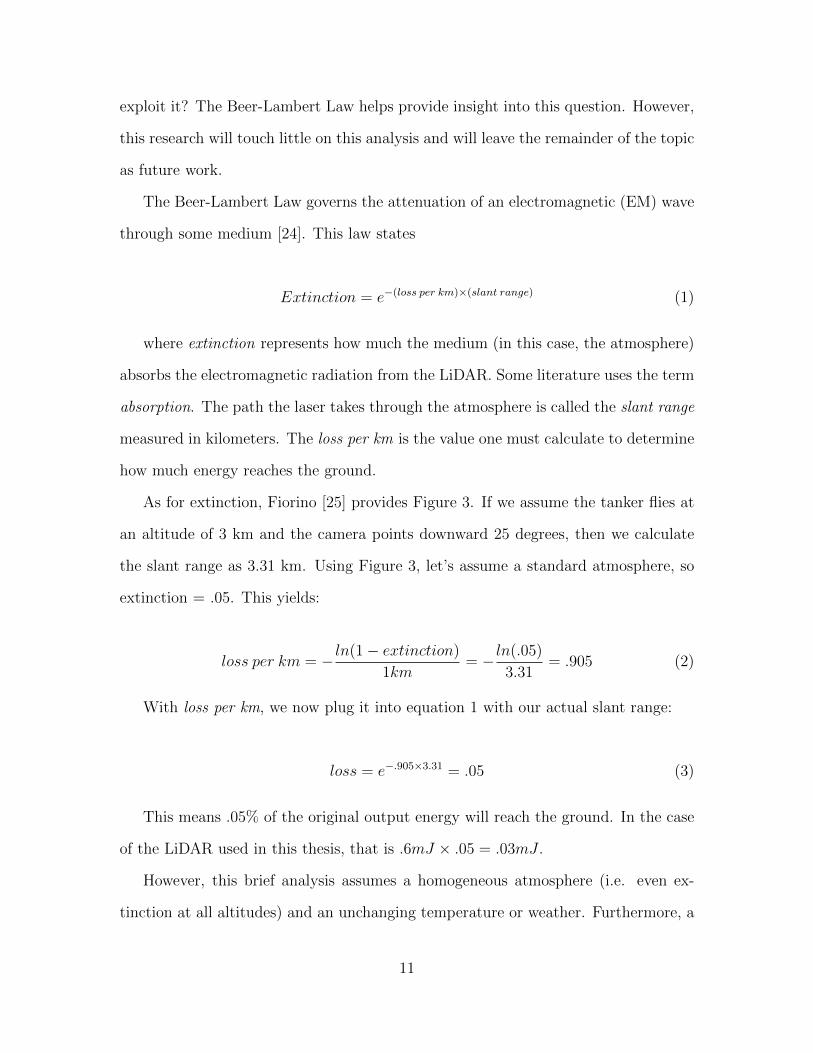
As for extinction, Fiorino [25] provides Figure 3. If we assume the tanker flies at

an altitude of 3 km and the camera points downward 25 degrees, then we calculate

the slant range as 3.31 km. Using Figure 3, let’s assume a standard atmosphere, so

extinction = .05. This yields:

loss per km = − ln(1− extinction)

1km= − ln(.05)

3.31= .905 (2)

With loss per km, we now plug it into equation 1 with our actual slant range:

loss = e−.905×3.31 = .05 (3)

This means .05% of the original output energy will reach the ground. In the case

of the LiDAR used in this thesis, that is .6mJ × .05 = .03mJ .

However, this brief analysis assumes a homogeneous atmosphere (i.e. even ex-

tinction at all altitudes) and an unchanging temperature or weather. Furthermore, a

11

Figure 3. How much loss an EM signal loses at various points on Earth

tanker will fly higher than 3km which only serves to limit the amount of energy that

reaches the ground. Many other factors also affect this analysis, but these assump-

tions help show that small enough energies will not pose an operational concern for

the tanker.

2.3.4 Global Registration Algorithms

A registration algorithm takes two input point clouds - a source and a target.

Throughout this research, we use the terms reference and sensed point clouds; in

this case, a registration algorithm aligns a reference onto a sensed point cloud. The

accuracy of this registration provides information on the 6 degrees of freedom (DOF)

of the sensed point cloud. In the case of AAR, these 6 DOF are crucial to the success

of the operation as they will help guide the boom to the UAV.

Many global registration algorithms exist, but this research only uses a few of the

most prolific algorithms.

12

2.3.4.1 Iterative Closest Point

Created in 1992 by Besl and McKay [1], ICP continually applies a rotation and

translation to a reference point cloud until it minimizes its objective function. This

function attempts to make the distance between each reference point and it’s closest

point in the sensed point cloud as small as possible.

The AftrBurner engine implements Besl’s original ICP algorithm but optimizes it

to minimize memory allocations and leverage modern coding paradigms. To differen-

tiate between this and other similarly-named algorithms, this research will refer to it

as Aftr ICP.

2.3.4.2 Point Cloud Library

The Point Cloud Library (PCL) is a standalone, large scale, open source project

for 2D/3D image and point cloud processing [26]. PCL provides a numerous utilities

for point cloud feature processing, filtering, registration, and segmentation. This

thesis employs the PCL registration functions.

PCL ICP expands upon the original ICP algorithm from 1992 and attempts to find

correspondences between points. It may then minimize the distance between these

correspondences, which eliminates the need to perform nearest neighbor queries as

discussed in Section 2.3.4.1; however, these correspondences require a similar amount

of computational complexity.

2.3.4.3 Fast Global Registration

Unlike PCL ICP or Aftr ICP, Fast Global Registration (FGR) calculates features

and normal vectors of the point cloud to find correspondences [3]. While FGR may

use any feature calculator, the original authors used Fast Point Feature Histograms

(FPFH), which produces 33 features of an input point cloud. While other feature

13

calculators exist, they produce hundreds of features, which negatively effect real-time

performance.

Based on these features, Figure 4 visualizes the correspondences the algorithm

makes; some are correct (blue) and some are incorrect (red).

Figure 4. Given a subset of the original image, FGR will form correspondences betweenthe sensed and reference point clouds

To help form these correspondences, FGR first downsamples the point cloud. PCL

provides a function called setLeafSize [27] that allows the user to specify the size of

a voxel. This 3D voxel will iterate over the point cloud and eliminate multiple points

per voxel.

Before and after picture of voxelization

2.3.4.4 Model-Based ICP (MBI) and Positions Perturbations Dif-

ference (PPD)

Curro [28] used MBI and PPD previously when working with an Ibeo scanning

LiDAR. A datasheet from the company’s website claims an accuracy of 10 cm inde-

pendent of distance [29], but Capt Curro’s results show RMSE of 33.9 cm and 39.1

cm for MBI and PPD, respectively.

2.3.5 Other LiDAR Performance

Curro [28] previously used an Ibeo Lux 8L LiDAR in his research at AFIT. Ibeo

advertises an accuracy of 10cm independent of distance [29], though Curro’s research

14

shows accuracies between 33cm and 39 cm.

Velodyne produces a large array of LiDAR products. One of which, the HDL-64E

S2, advertises an accuracy of 2cm for ”ambient wall tests” [30]. However, research

from Glennie [31] uses the HDL-64E and reports accuracies up to about 10cm; Glennie

also generated a ew calibration for the LiDAR that improved the accuracy to 3.5cm.

15

III. Methodology

To compare LiDAR to the current stereo vision system, the AftrBurner software

needed to interface with the EO and IR hardware. The EO and IR cameras run at

10 FPS while the LiDAR operates at 25 FPS. Conversely, the EO and IR cameras

capture a single frame in a matter of microseconds whereas the LiDAR captures a

frame in milliseconds. This timing disparity requires precise, asynchronous code to

gather the best possible data. With the proper timing, a pseudo refueling experiment

captured time-aligned data from all 3 cameras for post-processing and comparison.

3.1 LiDAR Data Format

The light detection and ranging (LiDAR) achieves a max frame rate up to 25

frames per second (FPS) with each frame composed of 32x128 pixels. Each pixel

carries 32 bits of range and intensity data for a total of 32x128x32 = 131072 bits

per frame. At the max frame rate of 25 FPS, that equates to 131072x25 = 3276800

bits/s, or 3.125 MB/s. Table 1 explains the composition of each pixel.

Because the LiDAR returns these convenient values, it allows for quick computa-

tion of the range to the target – the attribute on which this research places heavy

emphasis. At the max range, the data stream will read 0x0FFFF.FFF, which equates

to (210 − 1) +∑i=6

i=1 2−i = 1023.984375 feet. Conversely, the lowest value the LiDAR

will register is 2−6 = .015625 feet [32].

Range Fractional Range Intensity

31:28 27:24 23:20 19:16 15:12 11:8 7:4 3:0

0 0 0 0 29 28 27 26 25 24 23 22 21 20 2−1 2−2 2−3 2−4 2−5 2−6 211 210 29 28 27 26 25 24 23 22 21 20

Table 1. Bit organization of range and intensity values

16

3.2 LiDAR API

The LiDAR’s vendor-provided software lacked the flexibility required for use in

AAR; it did not allow for 3D visualization or the integration of registration or other

point cloud manipulation libraries. Further, it provided no compatibility with the

AftrBurner simulation engine. To overcome this, we developed an application pro-

gramming interface (API) to allow complete control over functionality of the camera.

The API exists within the AftrBurner engine, which enables direct visualization of

the data.

The programming manual that came with the LiDAR specifies several messages a

host processor must send to the camera in order to establish successful communica-

tions [32]. Table 2 lists the first five messages, known as the configuration commands,

which the camera requires after startup. After initialization, the host processor may

begin to send commands for a single frame or request a continuous series of frames

from the camera. Table 3 details these commands.

This API enables us to request frames from the LiDAR in conjunction with other

AAR code, which becomes very important when integrating the LiDAR with EO and

IR cameras. This level of control also allows us to verify the accuracy of the LiDAR,

which the next section will detail.

Message UDP Data Field Function1 0x10000001 00000011 FEEDBEEF Initialize host port addresses2 0x10000001 00000004 FFFFFFFF Configure camera registers3 0x10000001 0000000A 00000168 Number of pixels per packet4 0x10000001 0000000B 00010000 Frame buffer starting address5 0x10000001 0000000C 0000000B Number of packets sent for each frame

Table 2. Configuration command messages

17

Command UDP Data Field (hex) FunctionOne shot 0x10000001 00000301 00000099 Single frame

Run-at-rate 0x10000001 00000301 000000BF Continuous series of frames at max rateTerminate run-at-rate 0x10000001 00000301 00000098 Terminate the run-at-rate function

Table 3. Frame request messages

3.3 LiDAR Calibration

The baseline accuracy expected of this LiDAR comes from the Peregrine specifica-

tion datasheet [23]: 4 cm plus 1% of range. However, the LiDAR appeared to produce

inaccurate results in the lab. In the first tests, the camera consistently calculated a

distance 9-10 feet short of the measured distance. Figure ?? shows the initial setup

used to obtain these results. The hallway generated a large source of error in this

setup because the LiDAR pulses reflected off the walls and door frames to result in a

washed-out image. To produce a better LiDAR return, Figure 5 shows the improved

setup in a campus parking lot.

Figure 7 displays the results of these tests. An intermediate test between Figure

?? and Figure 5 took place on a street/sidewalk. This proved ineffective since the

heat of the sidewalk produced visible light distortions. In the final parking lot setup,

the camera looked down the row of parking spaces as a reference, and the cart in the

distance held a large, metal checkerboard. A survey wheel measured the true distance

from the camera to the edge of the cart, as shown on the x-axis in Figure 7.

Provide more details with the cold weather tests, discuss the fact that

the clock is not thermally controlled, which means a cold clock runs slower

and therefore calculates a shorter distance

18

Figure 5. Initial experiment setup

Figure 6. Refined setup

50 100 150 200 250 300 350 400Measured distance (meters)

25

20

15

10

5

0

Aver

age

Erro

r (m

eter

s)

Combined LiDAR Error Test ResultsAtriumStreetParking Lot 1Parking Lot 2

Figure 7. Results from the various LiDAR tests

3.4 LiDAR Field of View

The LiDAR’s narrow field of view (FOV) poses a problem for the normal ICP

algorithm. Figure 8 shows an accurate simulation of the LiDAR sensing a C-12 at 30

meters. To simulate LiDAR, the AftrBurner engine reads the virtual camera’s depth

19

buffer from the GPU and renders it directly to the screen as shown in the lower left

of Figure 8. AftrBurner linearly interpolates the value of each depth buffer pixel to a

range between 0 and 255; this creates a grayscale image in which closer points appear

darker and further points appear lighter.

Figure 8. A representation of the VFL’s field of view at 30 meters. The larger imageshows an optical perspective from a tanker while the smaller image in the bottom leftrepresents the LiDAR return data

With the depth buffer from Figure 8, the engine may construct a 3D point cloud.

To begin, one must understand what the depth map represents. Figure 9a displays

the near plane and far plane of a camera frustum; the camera can only view objects

between these two planes. For the Peregrine Flash LiDAR, the far plane lies at 1024

feet as discussed in Section 3.1. Figure 9b shows how a point at {x, y, z} in the 3D

space maps to a point {y′, z′} on the near plane, which corresponds to a pixel on the

computer screen. The value of each pixel in the bottom left of Figure 8 represents

the x-coordinate in 3D space.

A trigonometric construction helps compute the y and z from y′ and z′. Consider

the screen in Figure 10 – a small version of Figure 8’s depth buffer screen with the

20

(a) A 3D camera Frustum (b) Projection from 3D space to the near plane

Figure 9. A camera frustum. This will help construct geometric relationships toperform a 2D-to-3D projection.

same aspect ratio. Since the virtual flash LiDAR (VFL) is simulated as a pinhole

camera, imagine the pinhole exists at the center of the screen (blue dot).

Figure 10. Small LiDAR screen

Each pixel adds 15width

degrees from the center. Given a pixel (y’,z’), the generic

formula to calculate its angle from the center is:

φ =128

2− y − 0.5 (4)

θ =32

2− z − 0.5 (5)

21

Note the 0.5 will calculate the center of each pixel since the pinhole resides on

the line between pixels. For performance, the program precomputes a matrix of φ

and θ for every pixel. When required to project a 3D point cloud, the program uses

the geometric relationships in Figure 11 and Equations 6 and 7 to calculate the final

vector.

(a) (b)

Figure 11. The combined geometries of Figures 9b and 10

y = x× tan(φ) (6)

z =√x2 + y2 × tan(θ) (7)

Every pixel in the 2D depth map is now translated into a 3D vector. Figure 12

shows the representation of this point cloud in the AftrBurner engine, and Figure 13

displays a reprojection of real LiDAR data.

The point cloud in Figure 13 generated an expected amount of noise. To combat

this, OpenCV provides a function called medianBlur, which replaces each pixel with

the median of its neighboring pixels. Figure 14 shows the results of medianBlur.

Notice in Figure 14b how flat the point cloud becomes after medianBlur ; it looks like

it will perform well with the registration algorithms. Chapter IV will elaborate on

the registration results.

22

(a) (b)

Figure 12. The 3D point cloud in the virtual engine

(a) (b)

Figure 13. The 3D point cloud from real LiDAR data

3.5 Global Registration

This research uses three global registration algorithms: the original ICP [1], FGR

[3], and the well-known PCL ICP. Each algorithm uses mean squared error (MSE) to

gauge the quality of the registration as discussed in Section 3.7, and the AftrBurner

engine also tracks execution time. An ideal MSE is zero, which means a perfect 1-to-1

match for every point. At the same time, a faster execution time will enable real-time

AAR. As long as the algorithms execute under 100 ms to allow for 10 FPS, the MSE

23

(a) (b)

Figure 14. The real 3D point cloud after medianBlur

will be the most important factor to determine which algorithm to use.

In Figures 15-17, the yellow points represent the parts of the aircraft the VFL

senses and the red points represent the reference point cloud. These figures show

preliminary simulations with these algorithms; they do not take into account various

aircraft poses or sensor noise. These simulations only serve to prove the algorithms

work with representative data inside AftrBurner. Each registration algorithm com-

putes a rotation and translation that aligns the red points onto the yellow points.

(a) (b)

Figure 15. Aftr ICP results

24

(a) (b)

Figure 16. PCL ICP results

(a) (b)

Figure 17. FGR results

The simulations used a VFL with 128x512 resolution and a 15 degree FOV. The

algorithms first downsample each point cloud, then perform the registration, and last

compute the MSE between the yellow and red points. A comparison of the results

shows Aftr ICP in Figure 15 yields the best MSE and fastest execution time.

The simulation also generates noise to emulate the real LiDAR. Figures 18-20

display the same results as Figures 15-17 above but with a noisy point cloud. C++

offers a useful random normal distribution generator in the standard library. The

distribution used µ = 0 and σ = .2 in accordance with observed statistics with the

25

real LiDAR at 30 meters.

(a) (b)

Figure 18. Noisy Aftr ICP results

(a) (b)

Figure 19. Noisy PCL ICP results

Aftr ICP performed best again in both accuracy and execution time, but there

exists circumstances in which the other registration algorithms outperform Aftr ICP.

The next section will elaborate on one such scenario.

26

(a) (b)

Figure 20. Noisy FGR results

3.6 Fast Global Registration

FGR works best wdith partially-overlapping point clouds. Figure 21 shows one

such example. Each point cloud in this figure contains over 15,000 points, but FGR

excels if it first reduces that number; this process is known as downsampling through

use of the PCL library. To understand what sized voxel to use for downsampling, one

must analyze the volume of space a LiDAR pixel occupies at 30 meters, as this will

provide information on the disparity of the point cloud.

(a) (b)

Figure 21. Example point clouds

27

Each LiDAR pixel represented on Page 21 in Figure 10 exhibit the same arc as

they extend through space because every pixel extends .117 degrees horizontally and

vertically. Figure 22 shows the area a pixel will occupy at 30 meters.

Figure 22. Simple drawing of a LiDAR pixel extending 30 meters into space

This image helps define the length of the projected pixel as

1

2L = 30× tan(

.117

2) = .03

L = .06

(8)

Since the pixel projects into space as a square, we know the square must have an

area of .06m2. The PCL voxel will eliminate all but one point within each volume,

so this research used a voxel of 0.2m3 to eliminate about 23

of the pixels from both

point clouds. The authors of the FGR paper suggest a ratio of 1:2:5 for the voxel,

neighborhood search radius, and feature search radius, which translates to 0.2, 0.4,

and 1.0 respectively.

After downsampling, the yellow point cloud now contains 7911 points and the red

point cloud contains 7363 points.

When compared to ICP, the fact that the point clouds partially overlap proves a

28

(a) (b)

Figure 23. FGR registration with two partially-overlapping point clouds

detriment. ICP attempts to minimize the error between the points, but when some

part of the sensed point cloud never lines up with the reference point cloud, then ICP

will never converge. Figure 24 shows the same downsampled point clouds but with

ICP after 64 iterations; the results do not improve with more iterations.

(a) (b)

Figure 24. Aftr ICP registration with two partially-overlapping point clouds

Figure 25 provides the last demonstration on this data set. Unfortunately, it falls

short with only 64 iterations. Because PCL utilizes matched features between the

point clouds, the MSE calculation returns a number that’s better than the result

29

looks because the matched features align well with each other even if the other points

do not.

(a) (b)

Figure 25. PCL ICP registration with two partially-overlapping point clouds

FGR contains additional settings the fine-tune the performance of the algorithm.

However, this research used the default parameters:

• div factor = 1.4

• use absolute scale = 0

• max corr dist = .025

• iteration number = 64

• tuple scale = .95

• tuple max count = 1000

With these settings, Figure 26 provides a simulated between FGR and ICP for

this data.

3.7 Error Calculation

Both ICP and FGR utilize MSE to provide an apples-to-apples comparison. They

both also use a similar approach to calculate MSE – find a series correspondence

30

(a) (b)

Figure 26. Comparison between ICP and FGR

pairs, subtract each pair of points, square the magnitude, and divide by the total

number of points. However, the original FGR algorithm uses synthetic data which

provides access to the truth translation required to align the reference and sensed

point clouds. Unfortunately, the AAR application does not have that luxury.

This research copied part of the ICP code to compute MSE and leveraged a conve-

nient assumption given the nature of the problem domain. It starts by transforming

the reference points the algorithm produced onto the sensed points by means of the

rotation and translation. Then for each sensed point, it finds the nearest neighbor in

the reference point’s KD tree. Then for each pair of points, the algorithm subtracts

one from the other, squares the magnitude, then divides by the total number of sensed

points. Algorithm 1 formalizes this process. This algorithm assumes the sensed point

cloud will remain smaller than the reference point cloud; however, the presence of

water vapor clouds in the background may skew these results.

31

Algorithm 1 MSE Calculation for two point clouds (PC)

1: procedure MSE(sensedPoints, r, t)

2: mse← 0

3: temp← referencePoints

4: for i < temp.size() do . For each reference point

5: temp[i]← r ∗ temp[i] + t . Transform each point with the r and t

6: end for

7: refPC ← temp . Set the point cloud with the transformed points

8: for i < sensedPoints.size() do . For each sensed point

9: index← refPC.findNearestNeighbor(sensedPoints[i])

10: . Find the nearest point in the reference PC for each sensed point

11: mse = mse+ (sensedPoints[i]− refWO[index]).magnitudeSquared()

12: . Subtracting the two vectors yields another vector.

13: end for

14: mse = mse/sensedPoints.size() . Final MSE calculation

15: end procedure

3.8 Experiment Setup

The crux of this research focuses on the comparison between stereo vision and

LiDAR. In order to recreate Capt Will Dallman’s experiment [2], AFIT fabricated a

camera mount to include the flash LiDAR as seen in Figure 27. This mount places

each EO and each IR camera 12

meter apart – the same setup during previous test

flights.

Since a receiver flies about 100 feet from a tanker to refuel, this experiment placed

a wooden object 150 feet from the camera mount and moved the object toward the

cameras. Figure 28a and Figure 28b show the receiver and tanker, respectively.

32

(a) (b)

Figure 27. The cameras for the pseudo tanker

(a) (b)

Figure 28. The cameras for the pseudo tanker

Both EO and IR cameras receive a hardware trigger via USB. The EO cameras

operate at 10 Hz and the IR cameras operate at 30 Hz. The LiDAR will also operate

at 10 Hz, but it receives a trigger via UDP over Ethernet.

Once the system begins to collect truth data (discussed below in Sections 3.8.1

and 3.8.2), a multi-threaded program logs the data to a file. The other threads of this

program process data from each of the 5 cameras. These threads write information

about the received images to the same log file. In the case of the EO and IR cameras,

it writes the location of the saved image. For the LiDAR, it Base-64 encodes the raw

UDP data and writes the encoded string.

33

Since the LiDAR returns a complete image across 11 UDP packets, the thread

that saves LiDAR data timestamps the first packet. Once the thread receives the

final packet, it writes to the buffer corresponding to that timestamp; this ensures

synchronization between the LiDAR frames and the EO/IR images within the log

file.

For the actual exeriment, the two carts in Figures 28a and 28b face each other from

about 15 feet apart. The collection computer provides the triggers to all 5 cameras

and someone pushes the receive towards the tanker cameras. The images collected

from this simulated approach undergo post-processing. Post-processing must con-

sider camera calibration, pose estimation, and comparison of results between types

of cameras.

Each test with this setup consisted of three approaches:

1. Start at 15 meters from the tanker, back up to 50 meters, then move forward

to the starting position

2. Same as the first but stopping for 5 seconds at various reference points

3. Same as the first but with constant yawing in the receiver

3.8.1 Truth Source

A truth source must accompany the pose estimate of a receiver to validate the

experiment. This experiment used the Swift R©Piksi Multi - a multi-band, multi-

constellation real-time kinematics (RTK) Global Navigation Satellite System (GNSS)

receiver board that provides centimeter-level accurate positioning. It provides the

option to use GPS, GLONASS, BeiDou, and Galileo constellations [33]. To cre-

ate a DGPS solution, Piksi collects data from a rover (receiver) and base station

(tanker). Piksi may calculate the solution real-time given a communication link or

34

during post-processing. This experiment elected to post-process the DGPS solution

for two reasons: a radio link may drop packets, and a 150-meter ethernet cable proves

very difficult to manage.

Piksi samples GPS data at 5 Hz; unfortunately, it cannot sample at higher fre-

quencies. This produces some issues since our cameras collect twice as fast.

Chapter IV walks through the results of the stereo vision system and the LiDAR,

compare each to the truth data, and then compare them to each other.

3.8.2 GPS Time Server

To produce the most accurate results possible, each image from the stereo cameras

and LiDAR needs a GPS time stamp; this helps sync the entire system. This research

uses a TM2000A time server made by Time Machines Corp [34]. The TM2000A time

server uses a GPS antenna to receive a GPS signal and employs the precision time

protocol (PTP) and network time protocol (NTP). Together, these protocols enable

consistent, microsecond timing across our data collection.

Prior to imagery collection, the computer connects to the TM2000A via Ethernet.

Once connected, the internal clock for the data collection computer is synced with

the GPS time hosted on the TM2000A, which forces the data collection computer’s

clock to be accurate within 10−6 seconds. The TM2000A itself is hand-held in size

and requires a power connection to operate.

35

IV. Results

4.1 LiDAR Results

Initial results in Figure 29 show a decent point cloud up close when the receiver

is larger than the LiDAR frame. By virtue of testing on the ground, the LiDAR

produces a large quantity of points around the receiver. This required the use of a

point filter to eliminate the surrounding points, which in turn helps emulate a realistic

point cloud in the air.

(a) (b)

Figure 29. Point cloud playback with the real LiDAR

Once the receiver gets further away, it comes into full view of the LIDAR FOV.

Figure 30 shows what the point cloud looks like after filtering and medianBlur.

(a) (b)

Figure 30. LiDAR point cloud when receiver is in the full frame

36

4.2 ICP

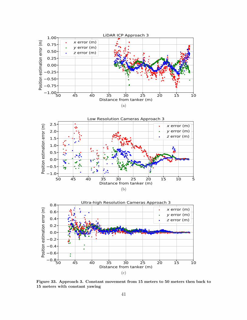
Due to the nature of LiDAR as discussed in Section 2.3.3.2, the results from this

research pale in comparison to stereo vision. Figures 31a-33a show results from the

three tests in Section 3.8. The low-resolution EO camera data comes from Dallmann

[2], and the high-resolution EO camera data comes from Lee [35].

The LiDAR data stops around 35 meters because the error continues to get worse

and the points extend beyond the boundaries of the filter. Even with a dynamic filter,

the error continues to grow and provides no new insight into the performance of the

LiDAR except for the fact that its accuracy decreases the further away a target moves

from the camera.

4.3 FGR

FGR requires correspondences between the sensed points and the reference points

to generate a valid pose registration. The more correspondences FGR finds the bet-

ter the pose registration. However, given a LiDAR with such a small resolution,

FGR continually fails to find the requisite number of correspondences and therefore

produces no registrations.

4.4 PCL

PCL’s implementation of Besl’s original ICP algorithm takes a similar approach

as FGR and uses correspondences to supplement the rest of the algorithm. However,

given the noise in the laser returns and therefore the resulting point cloud, PCL fails

to generate meaningful pose estimations due to erroneous correspondences.

37

4.5 Summary

The current Flash LiDAR technology AFIT bought produces too much noise to

support AAR. The lookup table (LUT) on the LiDAR is supposed to correct for these

discrepancies to a certain extent; however, it is a generalized LUT. A specialized LUT

will not be a viable option either. Across several tests, the LiDAR’s sensed values

at a specific range may vary greatly. For example, at 12.4 feet the LiDAR returned

11.11, 11.95, and 11.01 feet in 3 different tests. If a specialized LUT for the wooden

receiver added the average difference of these (1.04) to the returned value of each,

then then LiDAR would report 12.15, 12.99, and 12.05 respectively. At worst this

still provides a .59-foot error, or 17.98 centimeters.

LiDAR technology from other companies also experience a fair amount of noise in

their LiDAR data. In [31], Glennie shows that the Velodyne HDL-64E S2 scanning

LiDAR exhibits noise between -1.058 meters and 0.710 meters, but the distance at

which the LIDAR experiences these errors is unclear.

A separate Velodyne white paper [36] provides some information on the Velarray,

which claims to be the industry’s first 200 meter forward-looking LiDAR that can

detect objects with as little as 10% reflectivity. At this 200 meter range, the pa-

per claims an accuracy of ±3cm. Various Velodyne datasheets [37] [?] shows similar

accuracies for other products in their line, but careful reading suggests higher vari-

ance given longer range, higher reflectivity, and various environmental considerations.

Regarded as one of the current industry leaders in LiDAR technology, it appears Velo-

dyne LiDAR may not meet USAF needs either; however, tests similar to those in this

research will prove whether or not a LIDAR will meet various benchmarks required

for AAR.

38

101520253035404550Distance from tanker (m)

1.0

0.5

0.0

0.5

1.0Po

sition

estim

ation

erro

r (m)

LiDAR ICP Approach 1x error (m)y error (m)z error (m)

(a)

5101520253035404550Distance from tanker (m)

1.0

0.5

0.0

0.5

1.0

Posit

ion es

timati

on er

ror (

m)

Low Resolution Cameras Approach 1x error (m)y error (m)z error (m)

(b)

101520253035404550Distance from tanker (m)

0.80.60.40.20.00.20.40.60.8

Posit

ion es

timati

on er

ror (

m)

Ultra-high Resolution Cameras Approach 1x error (m)y error (m)z error (m)

(c)

Figure 31. Approach 1. Constant movement from 15 meters to 50 meters then back to15 meters

39

101520253035404550Distance from tanker (m)

0.80.60.40.20.00.20.40.60.8

Posit

ion es

timati

on er

ror (

m)LiDAR ICP Approach 2

x error (m)y error (m)z error (m)

(a)

5101520253035404550Distance from tanker (m)

0.5

0.0

0.5

1.0

Posit

ion es

timati

on er

ror (

m)

Low Resolution Cameras Approach 2x error (m)y error (m)z error (m)

(b)

101520253035404550Distance from tanker (m)

0.80.60.40.20.00.20.40.60.8

Posit

ion es

timati

on er

ror (

m)

Ultra-high Resolution Cameras Approach 2x error (m)y error (m)z error (m)

(c)

Figure 32. Approach 2. 15 meters to 50 meters then back to 15 meters, but stoppingfor 5 seconds at various points

40

101520253035404550Distance from tanker (m)

1.000.750.500.250.000.250.500.751.00

Posit

ion es

timati

on er

ror (

m)LiDAR ICP Approach 3

x error (m)y error (m)z error (m)

(a)

5101520253035404550Distance from tanker (m)

1.00.50.00.51.01.52.02.5

Posit

ion es

timati

on er

ror (

m)

Low Resolution Cameras Approach 3x error (m)y error (m)z error (m)

(b)

101520253035404550Distance from tanker (m)

0.80.60.40.20.00.20.40.60.8

Posit

ion es

timati

on er

ror (

m)

Ultra-high Resolution Cameras Approach 3x error (m)y error (m)z error (m)

(c)

Figure 33. Approach 3. Constant movement from 15 meters to 50 meters then back to15 meters with constant yawing

41

V. Conclusion

LiDAR presents a unique alternative to the current stereo vision method for AAR.

The nature of a LiDAR allows it to generate point clouds quicker, which already pro-

vides a benefit over EO or IR cameras as it cuts out the expensive SBM algorithm.

However, LiDAR will not work as a precision tool for AAR. Specifically, the Pere-

grine LiDAR does not produce consistent results that AAR demands for safety and

reliability.

5.1 Future Work

The ground tests presented a problem with extraneous points that will not exist

during flight; therefore, future research with LiDAR will benefit greatly from test

flights. Not only will test flights allow for the most realistic data, it may also address

how the curvatures of the aircraft will affect the lasers beams. Even on a flat metal

surface, the calculated distance becomes greater around the edges as beams diverge,

so an intricate surface will yield more interesting results.

On top of real test flights, a better LiDAR with a larger FOV may alleviate some

of the problems encountered in this research. At the same time, a LiDAR that utilizes

a different technology to generate a point cloud may also present useful progress for

AAR as discussed in Section 2.3.3.2. The Peregrine LiDAR takes a unique approach

to calculate distance; whether or not this methodology is what causes the inconsistent

point clouds is yet to be determined.

Further study might explore a material that returns the most reliable amount of

laser energy – one that will not attenuate or focus the beam too much. A laser beam

that maintains its wavelength may provide more consistent results with the current

LiDAR. This would translate to less perceived noise and make a specialized LUT a

42

more realistic possibility. At the same time, real UAVs likely will not use such a

material, which presents its own possibility for future work.

Only thorough research will address operational security concerns when using

LiDAR on a tanker. While a brief analysis shows the Peregrine LiDAR transmits

little energy to the ground from 10,000 feet, the USAF will benefit from an FOUO

report using various energies, different places of interest, and varying altitudes. The

analysis may also include time of year as the temperature and composition of the

atmosphere plays an important role in the Beer-Lambert law. The results of this

kind of analysis will help inform the USAF of any no-fly times for a LiDAR on a

tanker.

43

Appendix A. Video Replay of LiDAR Data

To access custom videos of the LIDAR data, see C:/repos/aar/students/michael.crowl/Crowl

Thesis/ThesisDefenseTemplate. The videos are titled Approach1.mp4, Approach2.mp4,

and Approach3.mp4. These videos show the data from Figures 31a-33a in Section 4.2.

These data come from the 13 January 2020 test located in X:/aar folder/stud/GroundTest/13 Jan 20.

Each video begins at pulse 100, and approaches 1, 2, and 3 run for 1400, 2000, and

1800 pulses respectively. As the cart gets further and further away, the LiDAR points

begin to drift outside the filter, which is why I limit the number of pulses.

The settings for start pulse and pulse duration are found within the configuration

file aftr.conf near the bottom. The specific variables are:

• TPS PlaybackLogFile

• TPS PlaybackLog EO Images

• TPS PlaybackLog IR Images

• TPSData Playback Option NumPulsesToConsume

• TPSData Playback Option TimeMode RealTime or EveryDatum

• TPSData Playback Option StartPulse

When you run aarViz, make sure TPS PlaybackLogFile in aftr.conf points to one

of the three log files located in X:/aar folder/stud/GroundTest/13 Jan 20/approach[1-

3] (that’s a regex to say approaches 1-3...).

44

Bibliography

1. P. J. Besl, “A Method for Registration of 3-D Shapes,” IEEE, vol. 14, no. 2,

pp. 239–256, 1992. [Online]. Available: https://www.sciencedirect.com/science/

article/pii/026288569290066C?via{\%}3Dihub

2. W. E. Dallmann, “INFRARED AND ELECTRO-OPTICAL STEREO VISION

FOR AUTOMATED AERIAL REFUELING,” 2018.

3. Q.-y. Zhou and J. Park, “Fast Global Registration.”

4. P. R. Thomas, U. Bhandari, S. Bullock, T. S. Richardson, and J. L. Du Bois,

“Advances in Air to Air Refuelling,” Progress in Aerospace Sciences, vol. 71, pp.

14–35, 2014.

5. J. P. Nalepka and J. L. Hinchman, “Automated Aerial Refueling : Extending the

Effectiveness of Unmanned Air Vehicles,” no. August, pp. 1–8, 2005.

6. B. S. Burns, “Autonomous Unmanned Aerial Vehicle Rendezvous for Automated

Aerial Refueling,” Ph.D. dissertation, 2007.

7. S. Nykl, C. Mourning, M. Leitch, D. Chelberg, T. Franklin, and C. Liu, “An

Overview of the STEAMiE Educational Game Engine,” no. November, 2008.

8. M. Winterbottom, C. Lloyd, J. Gaska, S. Wright, S. Hadley, O. Based, V. As-

sessment, O. Health, A. O. Branch, and P. Wing, “Stereoscopic Remote Vision

System Aerial Refueling Visual Performance,” pp. 1–10, 2016.

9. D. L. M. Ltd, “What can you use lidar for: How does lidar work,”

https://www.3dlasermapping.com/what-is-lidar-and-how-does-it-work/, 2019.

10. G. Vosselman and H.-G. Maas, Airborne and Terrestrial Laser Scanning.

Whittles, 2010. [Online]. Available: https://books.google.com/books?id=

YXNRPgAACAAJ

11. X. Zheng and C. Xiao, “Typical applications of airborne lidar technology in ge-

ological investigation,” International Archives of the Photogrammetry, Remote

Sensing and Spatial Information Sciences - ISPRS Archives, vol. 42, no. 3, pp.

2459–2463, 2018.

12. M. Dassot, T. Constant, and M. Fournier, “The use of terrestrial LiDAR tech-

nology in forest science: Application fields, benefits and challenges,” Annals of

Forest Science, vol. 68, no. 5, pp. 959–974, 2011.

45

13. V. Lidar, “Guide to LiDAR Wavelengths,” 2019. [Online]. Available:

https://velodynelidar.com/newsroom/guide-to-lidar-wavelengths/ [Accessed: 18

November 2019]

14. P. Crow, S. Benham, B. Devereux, and G. Amable, “Woodland vegetation

and its implications for archaeological survey using LiDAR,” Forestry: An

International Journal of Forest Research, vol. 80, no. 3, pp. 241–252, 07 2007.

[Online]. Available: https://doi.org/10.1093/forestry/cpm018

15. G. Amable, B. Devereux, P. Crow, and A. Cliff, “The potential of airborne lidar

for detection of archaeological features under woodland canopies,” Journal of

Archaeological Science, vol. 38, pp. 387–398, 02 2011.

16. S. Tan and J. Stoker, “Multiwavelength Polarimetric Lidar for

Foliage Obscured Man-Made Target Detection,” in Advances in

Geoscience and Remote Sensing, 2009. [Online]. Available: https:

//www.intechopen.com/books/advances-in-geoscience-and-remote-sensing/

multiwavelength-polarimetric-lidar-for-foliage-obscured-man-made-target-detection

17. November 2019, Thomas Welsh, Air Force Research Lab, Email interview.

18. X. Li, B. Yang, X. Xie, D. Li, and L. Xu, “Influence of waveform

characteristics on lidar ranging accuracy and precision,” Sensors (Basel,

Switzerland), vol. 18, no. 4, p. 1156, Apr 2018. [Online]. Available:

https://www.ncbi.nlm.nih.gov/pubmed/29642639

19. S. Bill, personal communication, November 2019, lead engineer at Advanced Sci-

entific Concepts.

20. A. S. M. A. Haseeb, F. Yusof, and H. H. Masjuki, “Laser-based Surface Modifica-

tions of Aluminum and its Alloys Laser-based Surface Modifications of Aluminum

and its Alloys,” no. October, 2015.

21. S. Sciencedirect, B. Making, and P. Bajpai, Biermann ’ s Handbook of Pulp and

Paper ( Third Chapter 11 - Optical Properties of Paper, 2018.

22. I. Juric, I. Karlovic, I. Tomic, and D. Novakovic, “Optical paper properties and

their influence on colour reproduction and perceived print quality,” vol. 28, no. 2,

2013.

23. A. S. C. Peregrine and F. Lidar, “Peregrine v2,” pp. 2–3.

24. J. Clark, “The Beer-lambert Law,” 2019.

46

25. S. T. Fiorino, R. J. Bartell, M. J. Krizo, D. J. Fedyk, P. Moore, T. R. Harris,

S. J. Cusumano, R. Richmond, and M. J. Gebhardt, “Worldwide assessments

of laser radar tactical scenario performance variability for diverse low altitude

atmospheric conditions at 1 . 0642 um and 1 . 557 um,” vol. 3, no. March, pp.

1–15, 2009.

26. R. B. Rusu and S. Cousins, “3D is here: Point Cloud Library (PCL),” in IEEE

International Conference on Robotics and Automation (ICRA), Shanghai, China,

May 9-13 2011.

27. PointClouds.org, “No Title,” 2018. [Online]. Available: http://docs.pointclouds.

org/1.8.1/classpcl{\ }1{\ }1{\ }voxel{\ }grid.html [Accessed: 2 November

2019]

28. J. A. Curro, “Automated Aerial Refueling Position Estimation Using

Scanning Flash LiDAR,” Ph.D. dissertation. [Online]. Available: https:

//apps.dtic.mil/dtic/tr/fulltext/u2/a562501.pdf

29. Hexagon, “ibeo LUX Data sheet,” 2017. [Online]. Avail-

able: https://autonomoustuff.com/wp-content/uploads/2019/05/ibeo{\ }LUX{\ }datasheet{\ }whitelabel.pdf

30. V. LiDAR, “HDL-64E,” Tech. Rep., 2018.

31. C. Glennie and D. D. Lichti, “Static Calibration and Analysis of the Velodyne

HDL-64E S2 for High Accuracy Mobile Scanning,” pp. 1610–1624, 2010.

32. Data Communication Programmer’s Guide for the Peregrine 3D Flash LiDAR

Camera, Advanced Scientific Concepts, LLC, 135 E. Ortega St., Santa Barbara,

Ca. 93101, August 2017.

33. S. Navigation, “Piksi Multi GNSS Module,” 2019. [Online]. Available:

https://www.swiftnav.com/piksi-multi [Accessed: 13 December 2019]

34. T. M. Corp, “Time machines,” https://timemachinescorp.com/, 2019.

35. A. Lee, “Placeholder title,” 2020.

36. W. Paper, “ASSISTANCE SYSTEMS WITH FORWARD-LOOKING LIDAR,”

no. May, 2019.

37. Velodyne LiDAR, “Puck Hi-Res,” Tech. Rep., 2019.

47