user’s guide ses software
TRANSCRIPT

User’s Guide
SES SOFTWARE

SES SOFTWARE User’s Guide v2.0
Copyright ©2014 VG Scienta AB
VG Scienta AB, P.O. Box 15120, 750 15 Uppsala, Sweden
Phone +46 18 480 58 00, Fax +46 18 555 888
E-mail: [email protected]
Web site: www.vgscienta.com
SES SOFTWARE User’s Guide v2.0 Copyright ©2014 VG Scienta AB
1
1 OVERVIEW
1.1 Introduction
The SES software is a Windows-based application that manages most of the user interaction with the SCIENTA spectrometer. The SES software controls the analyzer, and provides a plug-in interface for auxiliary equipment. This guide describes how to use the SES software, version 1.3.1.
1.2 Table of Contents
SES SOFTWARE .................................................................................................................................... 1 1 OVERVIEW ......................................................................................................................................... 1
1.1 Introduction ................................................................................................................................... 1 1.2 Table of Contents ......................................................................................................................... 1 1.3 History ............................................................................................................................................ 2
2 SECTION A – General Software Description ................................................................................ 3 2.1 Introduction ................................................................................................................................... 3 2.2 About the Software ....................................................................................................................... 3 2.3 How to Get Started with the Software ...................................................................................... 3 2.4 Main Menu ..................................................................................................................................... 4
3 SECTION C – Setup Dialogs ......................................................................................................... 11 3.1 Introduction ................................................................................................................................. 11 3.2 Global Detector Setup Dialog .................................................................................................. 11 3.3 Global vs Local Detector Settings ............................................................................................ 14 3.4 Signal Setup Dialog ..................................................................................................................... 15 3.5 File Options Dialog .................................................................................................................... 16 3.6 User Interfaces Dialog ............................................................................................................... 18 3.7 Excitation Energies Dialog ........................................................................................................ 19
4 SECTION D – Calibration Dialogs ............................................................................................... 22 4.1 Introduction ................................................................................................................................. 22 4.2 Voltage Calibration Dialog ........................................................................................................ 22 4.3 How to Optimize the Lens Deflection Elements .................................................................. 27 4.4 How to Edit Lens Tables ........................................................................................................... 28 4.5 Detector Calibration Dialog ...................................................................................................... 29 4.6 Spin Detector Calibration Dialog ............................................................................................. 32 4.7 Control Supplies Dialog ............................................................................................................. 35
5 SECTION E – Sequence Dialogs .................................................................................................. 37 5.1 Introduction ................................................................................................................................. 37 5.2 Sequence List Editor .................................................................................................................. 37 5.3 Sequence Editor .......................................................................................................................... 38 5.4 Region Editor .............................................................................................................................. 41 5.5 Run Modes ................................................................................................................................... 44 5.6 Special Regions ............................................................................................................................ 46
6 SECTION F – Operations during Acquisition ............................................................................ 47 6.1 Introduction ................................................................................................................................. 47 6.2 Operating the Spectrum Display .............................................................................................. 47 6.3 Sequence Tree ............................................................................................................................. 53 6.4 Status Bar ..................................................................................................................................... 54
SES SOFTWARE User’s Guide v2.0 Copyright ©2014 VG Scienta AB
2
7 SECTION G – Installations Dialogs ............................................................................................. 56 7.1 Introduction ................................................................................................................................. 56 7.2 Instrument Installation Dialog .................................................................................................. 56 7.3 Supply Installation Dialog.......................................................................................................... 58 7.4 Element Installation Dialog....................................................................................................... 59 7.5 Lens Mode Installation Dialog .................................................................................................. 60 7.6 Application Examples ................................................................................................................ 62
8 SECTION H – SES Options and Information Dialogs ............................................................. 66 8.1 Introduction ................................................................................................................................. 66 8.2 SES Options Dialog ................................................................................................................... 66 8.3 Supply Information Window .................................................................................................... 69 8.4 Detector Information Window ................................................................................................. 70
9 SECTION I – Manipulator ............................................................................................................. 72 9.1 Introduction ................................................................................................................................. 72 9.2 Installation.................................................................................................................................... 72 9.3 Setup ............................................................................................................................................. 73 9.4 Operation ..................................................................................................................................... 77
10 SECTION J – Monochromator .................................................................................................... 82 10.1 Introduction ............................................................................................................................... 82 10.2 Installation ................................................................................................................................. 82 10.3 Setup ........................................................................................................................................... 83 10.4 Operation ................................................................................................................................... 83
11 SECTION K – DA30 .................................................................................................................... 86 12 SECTION L – Single Transfer Spin ............................................................................................ 86
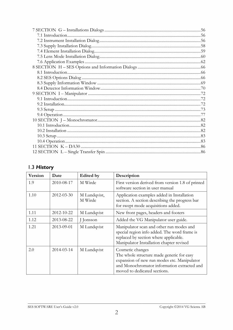
1.3 History
Version Date Edited by Description
1.9 2010-08-17 M Wirde First version derived from version 1.8 of printed software section in user manual
1.10 2012-03-30 M Lundqvist, M Wirde
Application examples added in Installation section. A section describing the progress bar for swept mode acquisitions added.
1.11 2012-10-22 M Lundqvist New front pages, headers and footers
1.12 2013-08-22 J Jonsson Added the VG Manipulator user guide.
1.21 2013-09-01 M Lundqvist Manipulator scan and other run modes and special region info added. The word frame is replaced by section where applicable. Manipulator Installation chapter revised
2.0 2014-03-14 M Lundqvist Cosmetic changes The whole structure made generic for easy expansion of new run modes etc. Manipulator and Monochromator information extracted and moved to dedicated sections.
SES SOFTWARE User’s Guide v2.0 Copyright ©2014 VG Scienta AB
3
2 SECTION A – General Software Description
2.1 Introduction
This section describes the system requirements, the recommended access control set-up and how to get started in the software.
2.2 About the Software
2.2.1 System Requirements
The SES software version 1.2.6 and earlier operates under Windows 2000 or Windows XP. Version 1.3.1 and later operates under Windows 7.
2.2.2 Access Control
The software enables a strict access control to sensitive calibration data by enabling a Privilege Level mechanism for individual voltage elements. The three levels available are: Administrator, Privileged User and User. The level is determined from the current Windows account, and the element access level is configured from the Element Installation dialog.
2.3 How to Get Started with the Software
2.3.1 Starting Program
The SES program is started by double-clicking on its icon. A click sound from the High Voltage should be noticeable.
2.3.2 Check Cables for Low or High Pass
The SES program begins with a pop-up window that reminds you to check cable connections for either Low Pass or High Pass.
2.3.3 Prior Runs
If the SES program has inadvertently shut down during prior acquisition and there is still usable data in the work folder, a query to save the data to an experiment file before continuing is displayed. Click Yes or No to continue.
2.3.4 Start Guide
Experiments are defined and started from the Setup and Run commands in the Sequence
menu (Sequence Setup and Sequence Run)
Energy calibration and lens deflection calibration is done in the Voltage Calibration dialog
(Calibration Voltages).
Global detector settings are defined through the Setup Global Detector command in the
Setup menu (Setup Global Detector).
SES SOFTWARE User’s Guide v2.0 Copyright ©2014 VG Scienta AB
4
2.3.5 Before Turning HV On
Make sure the pressure is below 110-5 mbar.
Open the Voltage Calibration dialog to check that the running parameters are reasonable
(Calibration Voltages).
Go to Chapter 3, System Operation.
2.4 Main Menu
2.4.1 Introduction
This section gives an overview of the commands that are found in the SES main menu (the SES menu bar).
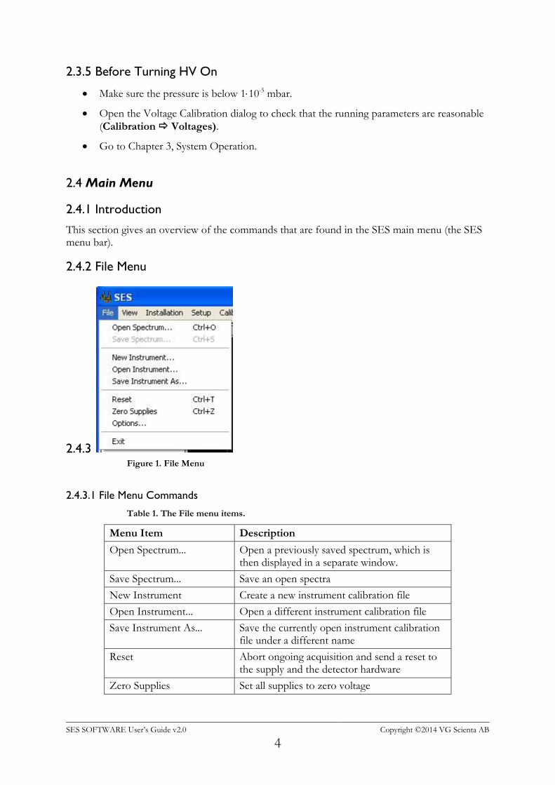
2.4.2 File Menu
2.4.3 Figure 1. File Menu
2.4.3.1 File Menu Commands
Table 1. The File menu items.
Menu Item Description
Open Spectrum... Open a previously saved spectrum, which is then displayed in a separate window.
Save Spectrum... Save an open spectra
New Instrument Create a new instrument calibration file
Open Instrument... Open a different instrument calibration file
Save Instrument As... Save the currently open instrument calibration file under a different name
Reset Abort ongoing acquisition and send a reset to the supply and the detector hardware
Zero Supplies Set all supplies to zero voltage
SES SOFTWARE User’s Guide v2.0 Copyright ©2014 VG Scienta AB
5
Options... Open the SES Options dialog
Exit Close the SES program
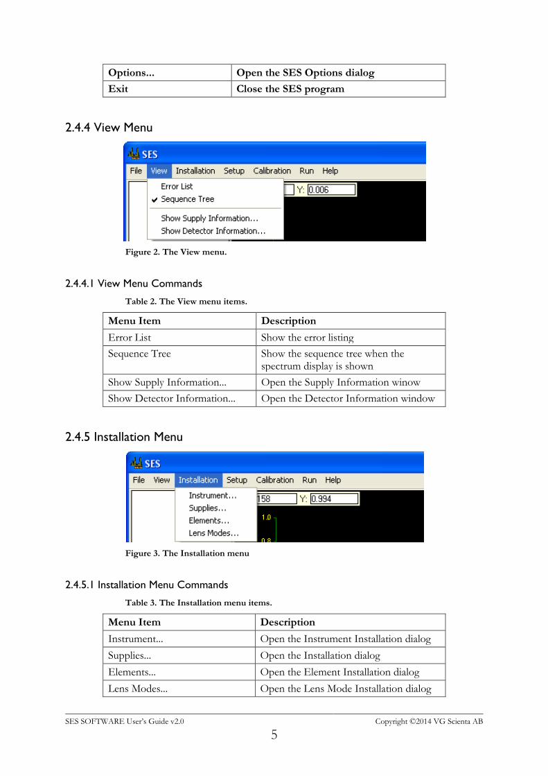
2.4.4 View Menu
Figure 2. The View menu.
2.4.4.1 View Menu Commands
Table 2. The View menu items.
Menu Item Description
Error List Show the error listing
Sequence Tree Show the sequence tree when the spectrum display is shown
Show Supply Information... Open the Supply Information winow
Show Detector Information... Open the Detector Information window
2.4.5 Installation Menu
Figure 3. The Installation menu
2.4.5.1 Installation Menu Commands
Table 3. The Installation menu items.
Menu Item Description
Instrument... Open the Instrument Installation dialog
Supplies... Open the Installation dialog
Elements... Open the Element Installation dialog
Lens Modes... Open the Lens Mode Installation dialog
SES SOFTWARE User’s Guide v2.0 Copyright ©2014 VG Scienta AB
6
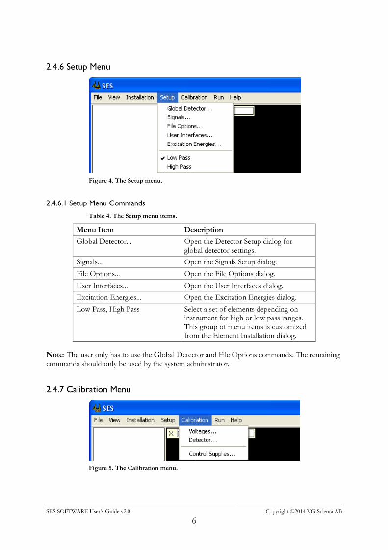
2.4.6 Setup Menu
Figure 4. The Setup menu.
2.4.6.1 Setup Menu Commands
Table 4. The Setup menu items.
Menu Item Description
Global Detector... Open the Detector Setup dialog for global detector settings.
Signals... Open the Signals Setup dialog.
File Options... Open the File Options dialog.
User Interfaces... Open the User Interfaces dialog.
Excitation Energies... Open the Excitation Energies dialog.
Low Pass, High Pass Select a set of elements depending on instrument for high or low pass ranges. This group of menu items is customized from the Element Installation dialog.
Note: The user only has to use the Global Detector and File Options commands. The remaining commands should only be used by the system administrator.
2.4.7 Calibration Menu
Figure 5. The Calibration menu.
SES SOFTWARE User’s Guide v2.0 Copyright ©2014 VG Scienta AB
7
2.4.7.1 Calibration Menu Commands
Table 5. The Calibration menu items.
Menu Item Description
Voltages... Open the Voltage Calibration dialog.
Detector... Open the Detector Calibration dialog.
Control Supplies... Open the Control Supplies dialog.
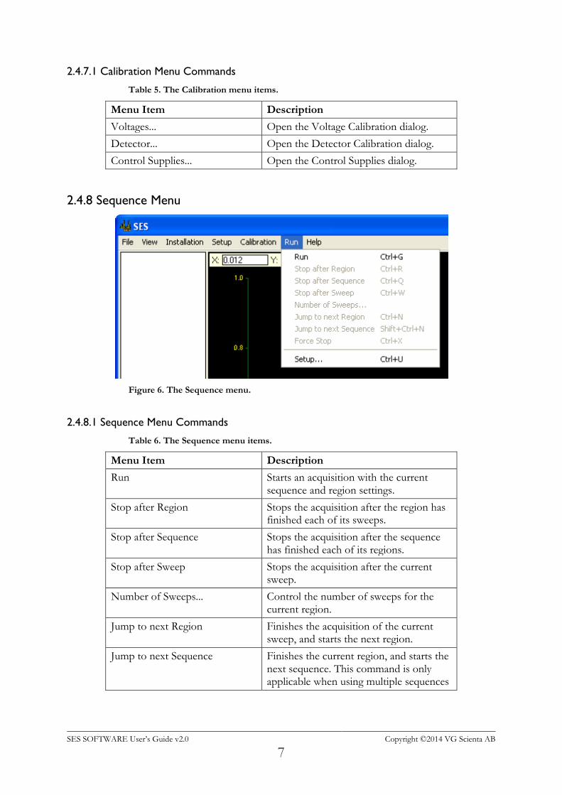
2.4.8 Sequence Menu
Figure 6. The Sequence menu.
2.4.8.1 Sequence Menu Commands
Table 6. The Sequence menu items.
Menu Item Description
Run Starts an acquisition with the current sequence and region settings.
Stop after Region Stops the acquisition after the region has finished each of its sweeps.
Stop after Sequence Stops the acquisition after the sequence has finished each of its regions.
Stop after Sweep Stops the acquisition after the current sweep.
Number of Sweeps... Control the number of sweeps for the current region.
Jump to next Region Finishes the acquisition of the current sweep, and starts the next region.
Jump to next Sequence Finishes the current region, and starts the next sequence. This command is only applicable when using multiple sequences
SES SOFTWARE User’s Guide v2.0 Copyright ©2014 VG Scienta AB
8
Cancel Stop Cancels the current stop request. This command is available only after one of the above stop requests has been issued.
Force Stop Forces the current acquisition to stop immediately. Incomplete data from the current sweep is discarded, but data from earlier sweeps is kept.
Setup... When using multiple sequences, opens the Sequence List Editor for acquisition setup. Otherwise, opens the Sequence Editor.
Note: If the Autosave option is checked in the File Options dialog, all stop commands will save acquired data. Note: If the Zero voltages option is checked in the Acquisition tab of the SES Options dialog, Force Stop works effectively as an emergency button, resetting all supplies to zero. This is important when working with experiments which might damage the detector.
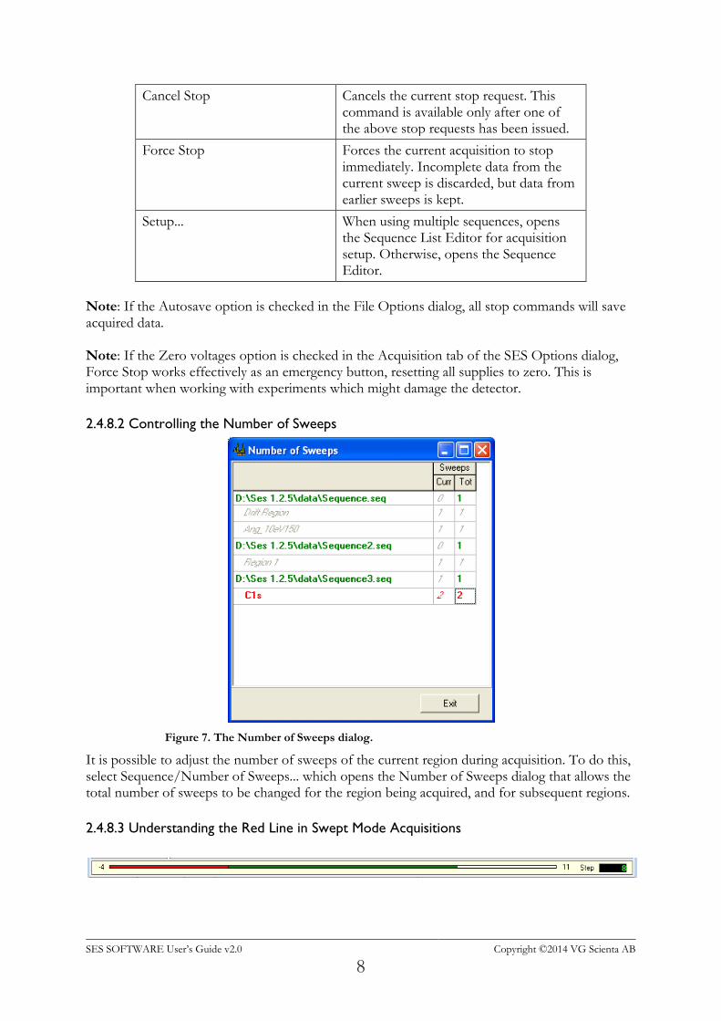
2.4.8.2 Controlling the Number of Sweeps
Figure 7. The Number of Sweeps dialog.
It is possible to adjust the number of sweeps of the current region during acquisition. To do this, select Sequence/Number of Sweeps... which opens the Number of Sweeps dialog that allows the total number of sweeps to be changed for the region being acquired, and for subsequent regions.
2.4.8.3 Understanding the Red Line in Swept Mode Acquisitions
SES SOFTWARE User’s Guide v2.0 Copyright ©2014 VG Scienta AB
9
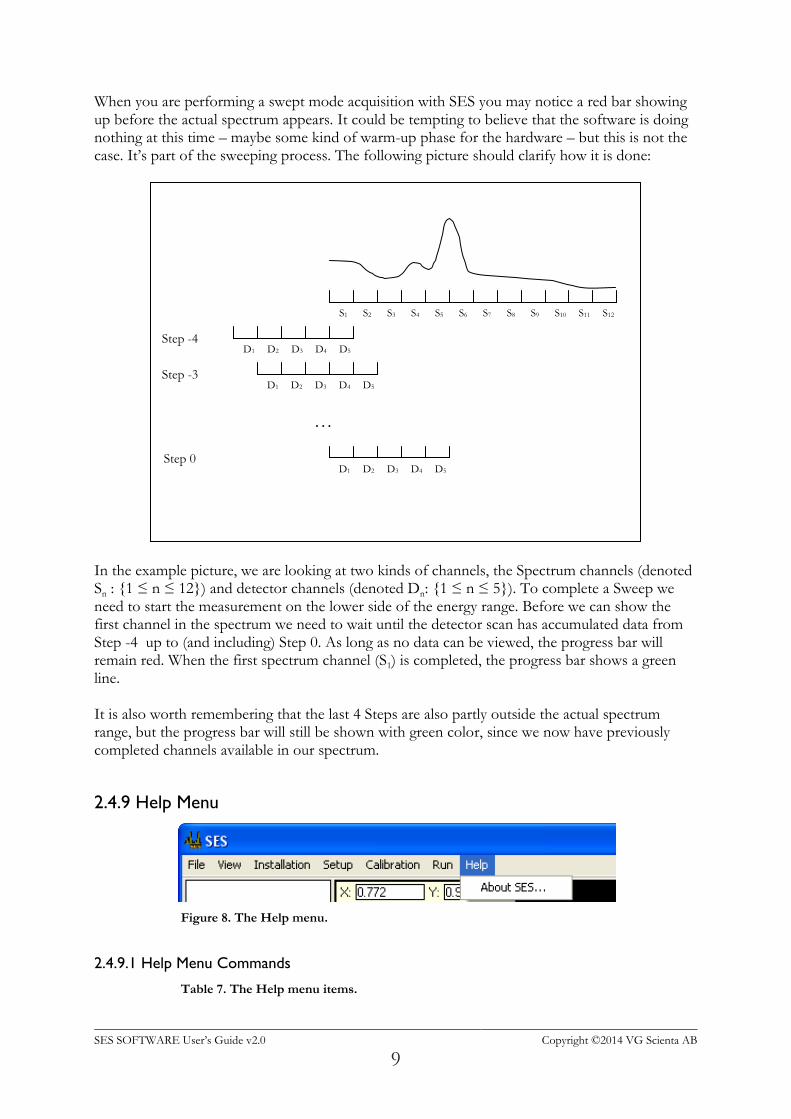
When you are performing a swept mode acquisition with SES you may notice a red bar showing up before the actual spectrum appears. It could be tempting to believe that the software is doing nothing at this time – maybe some kind of warm-up phase for the hardware – but this is not the case. It’s part of the sweeping process. The following picture should clarify how it is done:
In the example picture, we are looking at two kinds of channels, the Spectrum channels (denoted Sn : {1 ≤ n ≤ 12}) and detector channels (denoted Dn: {1 ≤ n ≤ 5}). To complete a Sweep we need to start the measurement on the lower side of the energy range. Before we can show the first channel in the spectrum we need to wait until the detector scan has accumulated data from Step -4 up to (and including) Step 0. As long as no data can be viewed, the progress bar will remain red. When the first spectrum channel (S1) is completed, the progress bar shows a green line. It is also worth remembering that the last 4 Steps are also partly outside the actual spectrum range, but the progress bar will still be shown with green color, since we now have previously completed channels available in our spectrum.
2.4.9 Help Menu
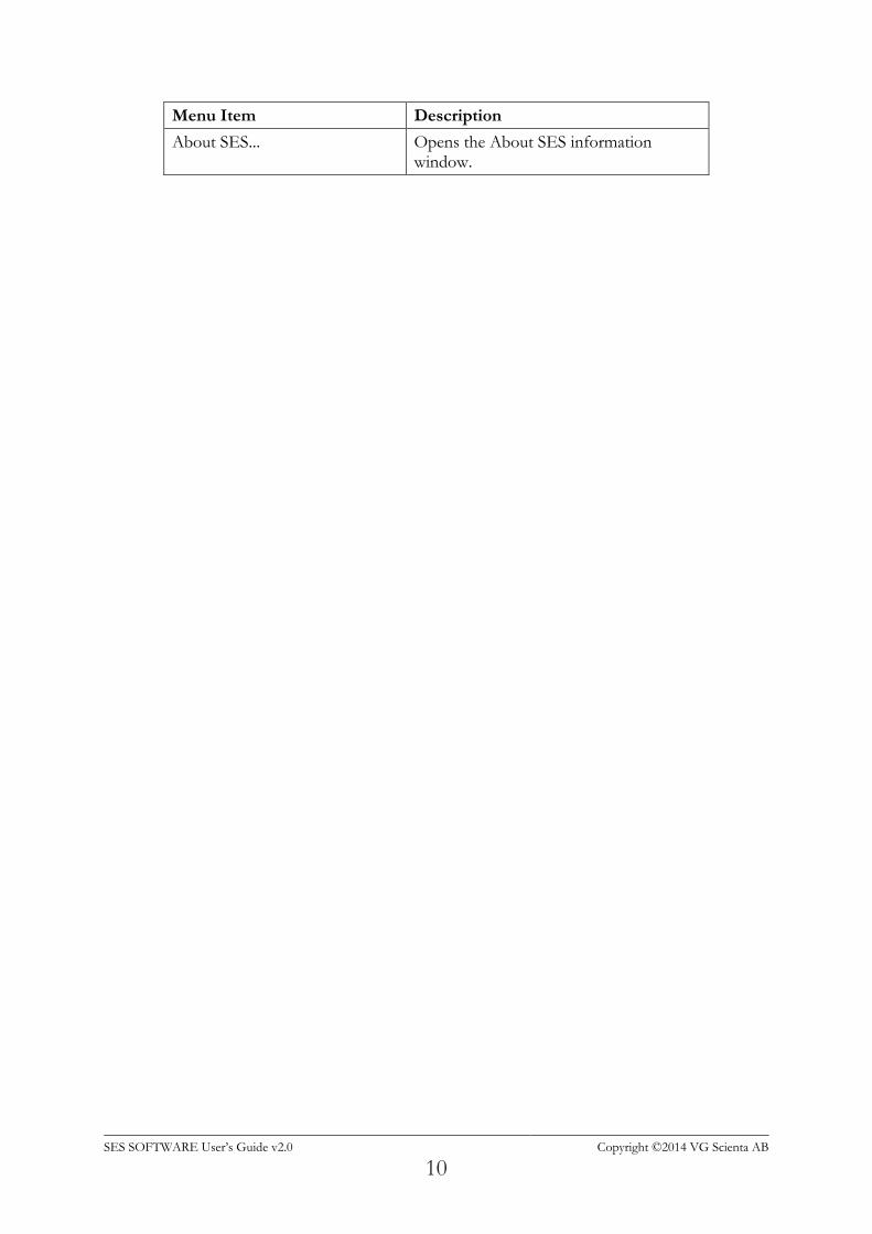
Figure 8. The Help menu.
2.4.9.1 Help Menu Commands
Table 7. The Help menu items.
S1 S2 S3 S4 S5 S6 S7 S8 S9 S10 S11 S12
D1 D2 D3 D4 D5
D1 D2 D3 D4 D5
D1 D2 D3 D4 D5
…
Step -4
Step -3
Step 0
SES SOFTWARE User’s Guide v2.0 Copyright ©2014 VG Scienta AB
10
Menu Item Description
About SES... Opens the About SES information window.
SES SOFTWARE User’s Guide v2.0 Copyright ©2014 VG Scienta AB
11
3 SECTION C – Setup Dialogs
3.1 Introduction
This section describes how to use the Setup dialogs.
3.2 Global Detector Setup Dialog
3.2.1 Description
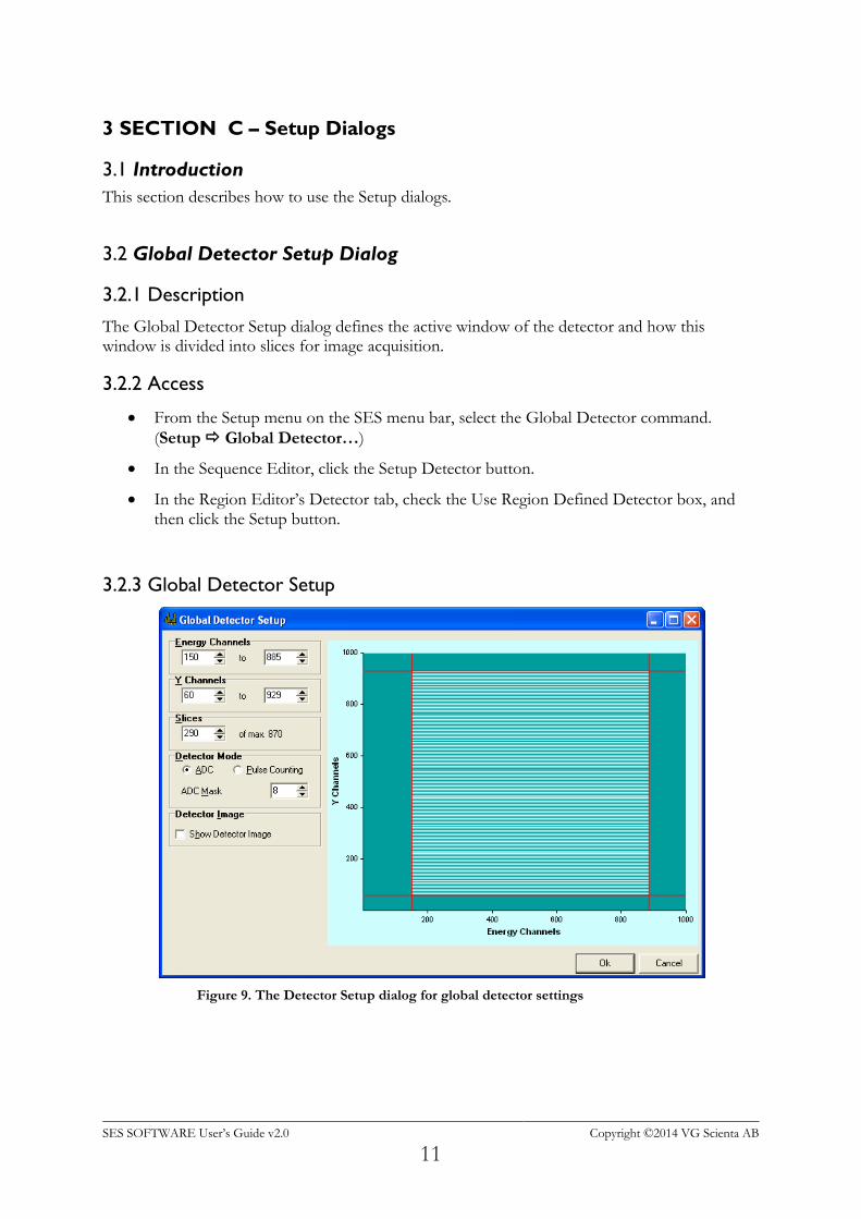
The Global Detector Setup dialog defines the active window of the detector and how this window is divided into slices for image acquisition.
3.2.2 Access
From the Setup menu on the SES menu bar, select the Global Detector command.
(Setup Global Detector…)
In the Sequence Editor, click the Setup Detector button.
In the Region Editor’s Detector tab, check the Use Region Defined Detector box, and then click the Setup button.
3.2.3 Global Detector Setup
Figure 9. The Detector Setup dialog for global detector settings
SES SOFTWARE User’s Guide v2.0 Copyright ©2014 VG Scienta AB
12
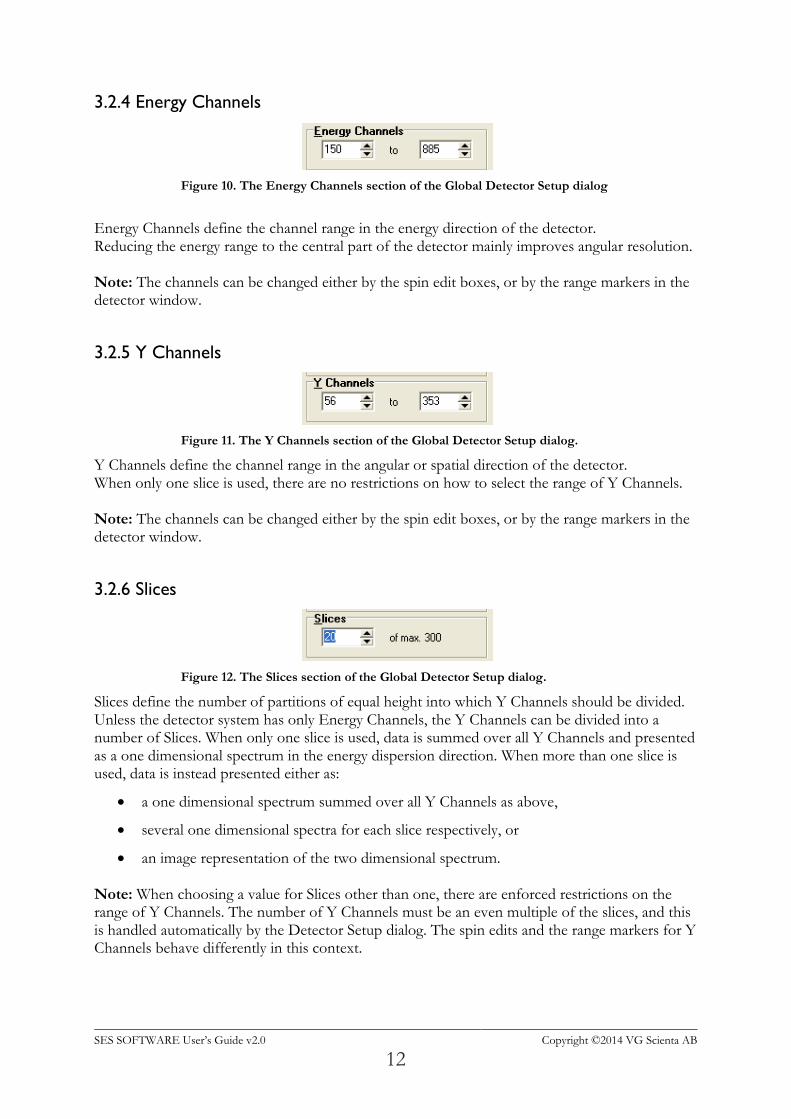
3.2.4 Energy Channels
Figure 10. The Energy Channels section of the Global Detector Setup dialog
Energy Channels define the channel range in the energy direction of the detector. Reducing the energy range to the central part of the detector mainly improves angular resolution. Note: The channels can be changed either by the spin edit boxes, or by the range markers in the detector window.
3.2.5 Y Channels
Figure 11. The Y Channels section of the Global Detector Setup dialog.
Y Channels define the channel range in the angular or spatial direction of the detector. When only one slice is used, there are no restrictions on how to select the range of Y Channels. Note: The channels can be changed either by the spin edit boxes, or by the range markers in the detector window.
3.2.6 Slices
Figure 12. The Slices section of the Global Detector Setup dialog.
Slices define the number of partitions of equal height into which Y Channels should be divided. Unless the detector system has only Energy Channels, the Y Channels can be divided into a number of Slices. When only one slice is used, data is summed over all Y Channels and presented as a one dimensional spectrum in the energy dispersion direction. When more than one slice is used, data is instead presented either as:
a one dimensional spectrum summed over all Y Channels as above,
several one dimensional spectra for each slice respectively, or
an image representation of the two dimensional spectrum. Note: When choosing a value for Slices other than one, there are enforced restrictions on the range of Y Channels. The number of Y Channels must be an even multiple of the slices, and this is handled automatically by the Detector Setup dialog. The spin edits and the range markers for Y Channels behave differently in this context.
SES SOFTWARE User’s Guide v2.0 Copyright ©2014 VG Scienta AB
13
3.2.7 Detector Modes
Detector Mode defines whether the detector system should use Pulse Counting or ADC mode. The detector systems based on the VG Scienta 7059 processor cards and newer detector systems based on FireWire cameras have two detector modes; ADC and Pulse Counting mode. Older detector systems may have either Pulse Counting mode, or no modes.
3.2.8 ADC Mode
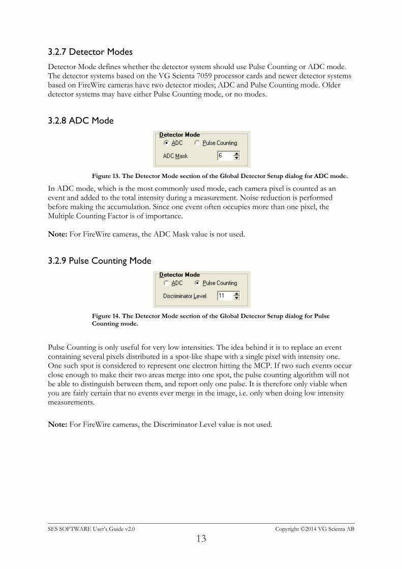
Figure 13. The Detector Mode section of the Global Detector Setup dialog for ADC mode.
In ADC mode, which is the most commonly used mode, each camera pixel is counted as an event and added to the total intensity during a measurement. Noise reduction is performed before making the accumulation. Since one event often occupies more than one pixel, the Multiple Counting Factor is of importance. Note: For FireWire cameras, the ADC Mask value is not used.
3.2.9 Pulse Counting Mode
Figure 14. The Detector Mode section of the Global Detector Setup dialog for Pulse Counting mode.
Pulse Counting is only useful for very low intensities. The idea behind it is to replace an event containing several pixels distributed in a spot-like shape with a single pixel with intensity one. One such spot is considered to represent one electron hitting the MCP. If two such events occur close enough to make their two areas merge into one spot, the pulse counting algorithm will not be able to distinguish between them, and report only one pulse. It is therefore only viable when you are fairly certain that no events ever merge in the image, i.e. only when doing low intensity measurements.
Note: For FireWire cameras, the Discriminator Level value is not used.
SES SOFTWARE User’s Guide v2.0 Copyright ©2014 VG Scienta AB
14
3.2.10 Detector Image
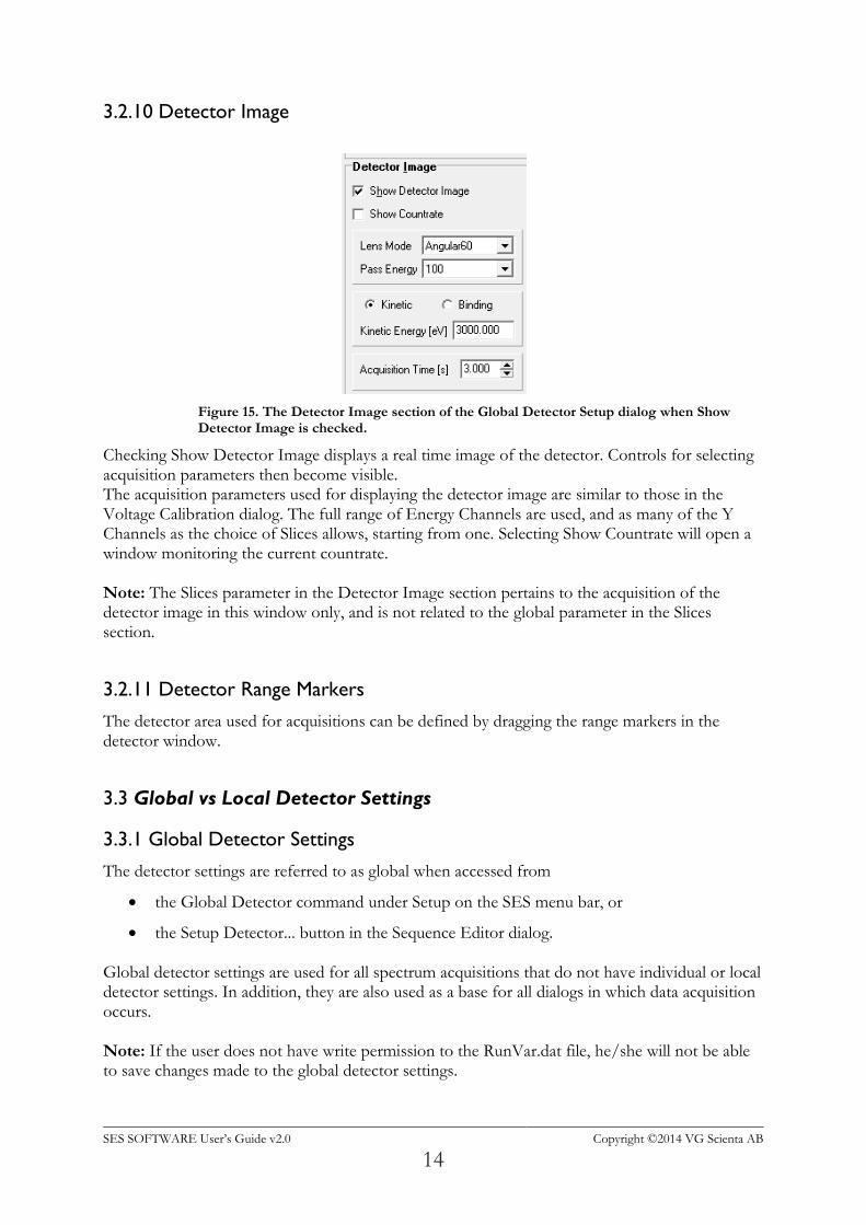
Figure 15. The Detector Image section of the Global Detector Setup dialog when Show Detector Image is checked.
Checking Show Detector Image displays a real time image of the detector. Controls for selecting acquisition parameters then become visible. The acquisition parameters used for displaying the detector image are similar to those in the Voltage Calibration dialog. The full range of Energy Channels are used, and as many of the Y Channels as the choice of Slices allows, starting from one. Selecting Show Countrate will open a window monitoring the current countrate. Note: The Slices parameter in the Detector Image section pertains to the acquisition of the detector image in this window only, and is not related to the global parameter in the Slices section.
3.2.11 Detector Range Markers
The detector area used for acquisitions can be defined by dragging the range markers in the detector window.
3.3 Global vs Local Detector Settings
3.3.1 Global Detector Settings
The detector settings are referred to as global when accessed from
the Global Detector command under Setup on the SES menu bar, or
the Setup Detector... button in the Sequence Editor dialog. Global detector settings are used for all spectrum acquisitions that do not have individual or local detector settings. In addition, they are also used as a base for all dialogs in which data acquisition occurs. Note: If the user does not have write permission to the RunVar.dat file, he/she will not be able to save changes made to the global detector settings.
SES SOFTWARE User’s Guide v2.0 Copyright ©2014 VG Scienta AB
15
3.3.2 Local Detector Settings
The detector settings are referred to as local when accessed from the Region Editor by checking the Use Region Defined Detector box and then clicking the corresponding Setup button.
3.4 Signal Setup Dialog
3.4.1 Description
The Setup Detector dialog defines the active window of the detector and how this window is divided into slices for image acquisition.
3.4.2 Access
From the Setup menu on the SES menu bar, select the Signals command. (Setup Signals…)
3.4.3 Signal Setup
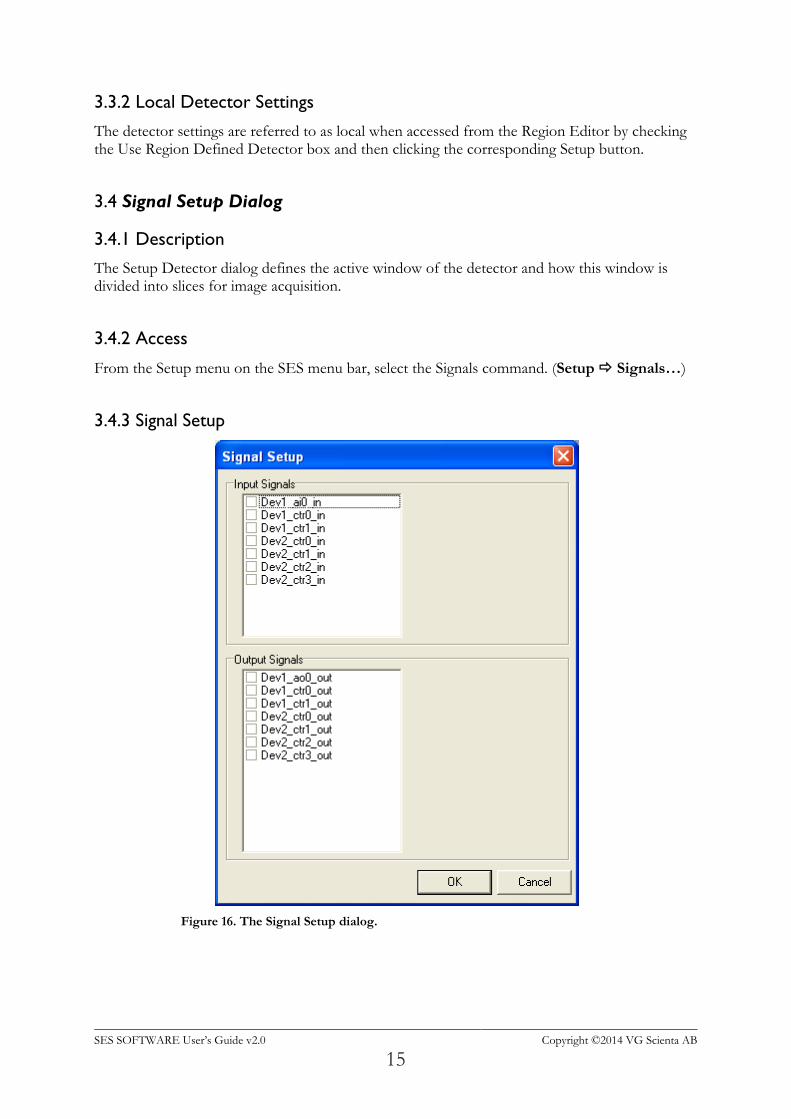
Figure 16. The Signal Setup dialog.
SES SOFTWARE User’s Guide v2.0 Copyright ©2014 VG Scienta AB
16
3.4.4 Input Signals
The Input Signals section lists the input channels defined in the I/O interface library. Input signals can be disabled individually by clicking the check boxes next to the corresponding signal name.
3.4.5 Output Signals
The Output Signals section lists the input channels defined in the I/O interface library. Output signals can be disabled individually by clicking the check boxes next to the corresponding signal name.
3.5 File Options Dialog
3.5.1 Description
The File Options dialog is used for specifying available experiment file libraries and for defining parameters such as experiment file-type, save directory and file naming method.
3.5.2 Access
From the Setup menu on the SES menu bar, select the File Options command.
(Setup File Options…)
In the Sequence Editor click the File Options button. Note: When using multiple sequences and accessing the File Options dialog from the Setup menu, the file options for the first sequence in the list are displayed.
SES SOFTWARE User’s Guide v2.0 Copyright ©2014 VG Scienta AB
17
3.5.3 File Options
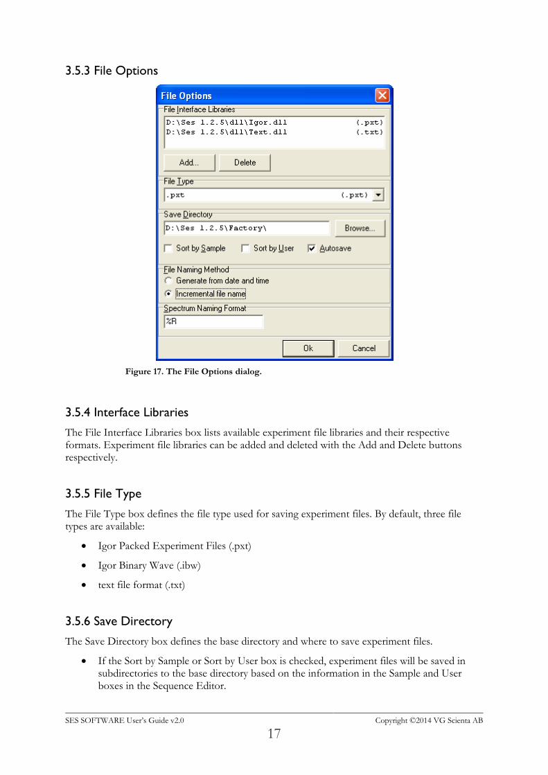
Figure 17. The File Options dialog.
3.5.4 Interface Libraries
The File Interface Libraries box lists available experiment file libraries and their respective formats. Experiment file libraries can be added and deleted with the Add and Delete buttons respectively.
3.5.5 File Type
The File Type box defines the file type used for saving experiment files. By default, three file types are available:
Igor Packed Experiment Files (.pxt)
Igor Binary Wave (.ibw)
text file format (.txt)
3.5.6 Save Directory
The Save Directory box defines the base directory and where to save experiment files.
If the Sort by Sample or Sort by User box is checked, experiment files will be saved in subdirectories to the base directory based on the information in the Sample and User boxes in the Sequence Editor.
SES SOFTWARE User’s Guide v2.0 Copyright ©2014 VG Scienta AB
18
If the Autosave box is checked, experiment data will be saved after each time that the sequence has completed an execution. Experiment data will then also be saved when the sequence is stopped by the user.
3.5.7 File Naming Method
File Naming Method defines whether experiment file names should be constructed from the date and time of the acquisition, or from an incremental number. The file names generated from date and time have the format base-mmddhhnn.ext while the file names generated from an incremental number have the format base-xxx.ext.
3.5.8 Spectrum Naming Format
The Spectrum Naming Format box defines how the spectra are named in the experiment files. There are three format parameters:
%R represents the region name
%F represents the experiment file name
%N represents the incremental number or date and time of the experiment file name Example: ‘%R_%N’ would name the spectrum ‘Region1_001’ for a region with name ‘Region1’ and incremental number ‘001’.
3.6 User Interfaces Dialog
3.6.1 Description
The User Interfaces dialog is used to load and unload plug-ins or user interface libraries for auxiliary equipment, such as sample manipulator, monochromator, flood gun and ion gun. Loaded plug-ins are listed in the Loaded User Interfaces section. A user interface defines so called Run Modes and/or Special Regions that are handled from the Sequence Editor when an experiment is setup.
3.6.2 Access
From the Setup menu on the SES menu bar, select the User Interfaces command. (Setup User Interfaces…)
SES SOFTWARE User’s Guide v2.0 Copyright ©2014 VG Scienta AB
19
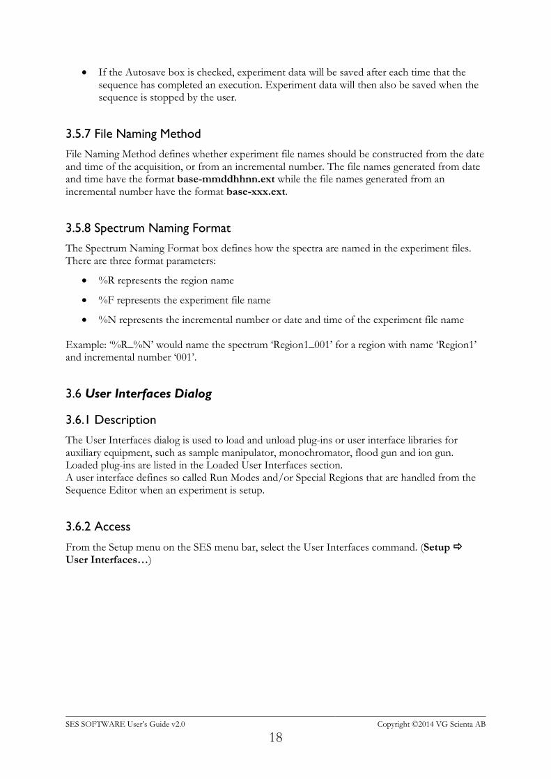
3.6.3 User Interfaces
Figure 18. The User Interfaces dialog
Note: This dialog should only be used by the system administrator.
3.6.4 Add, Delete and Setup Buttons
New User Interface plug-ins can be loaded by clicking the Add button and browse for the desired plug-in.
A plug-in can be unloaded by selecting it in the list and clicking the Delete button.
If the selected plug-in has a setup dialog, it can be opened by clicking the Setup button. As an example: The general manipulator library plug-in has a setup dialog where a hardware dependent library for a particular motor type is selected.
3.7 Excitation Energies Dialog
3.7.1 Description
The Excitation Energies dialog is used to define excitation energies, specify default excitation energy and to change the current excitation energy.
3.7.2 Access
From the Setup menu on the SES menu bar, select the Excitation Energies command. (Setup Excitation Energies…)
SES SOFTWARE User’s Guide v2.0 Copyright ©2014 VG Scienta AB
20
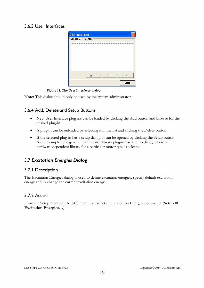
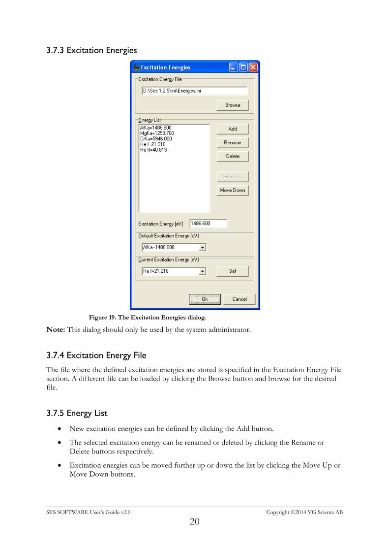
3.7.3 Excitation Energies
Figure 19. The Excitation Energies dialog.
Note: This dialog should only be used by the system administrator.
3.7.4 Excitation Energy File
The file where the defined excitation energies are stored is specified in the Excitation Energy File section. A different file can be loaded by clicking the Browse button and browse for the desired file.
3.7.5 Energy List
New excitation energies can be defined by clicking the Add button.
The selected excitation energy can be renamed or deleted by clicking the Rename or Delete buttons respectively.
Excitation energies can be moved further up or down the list by clicking the Move Up or Move Down buttons.
SES SOFTWARE User’s Guide v2.0 Copyright ©2014 VG Scienta AB
21
The actual energy for the selected excitation energy can be changed in the Excitation Energy field.
3.7.6 Default Excitation Energy
The Default Excitation Energy section specifies which excitation energy to use when creating new regions. The default excitation energy can be changed either by selecting a predefined energy from the drop-down list or by entering a new value.
3.7.7 Current Excitation Energy
The Current Excitation Energy section specifies the excitation energy currently assigned to the instrument. The current excitation energy can be changed by either selecting one of the predefined excitation energies from the drop-down list or by entering a new value and clicking the Set button. Note: If a monochromator plug-in is loaded, the Current Excitation Energy section will display the current photon energy of the monochromator. When the current excitation energy is changed, the new value is assigned to the monochromator.
SES SOFTWARE User’s Guide v2.0 Copyright ©2014 VG Scienta AB
22
4 SECTION D – Calibration Dialogs
4.1 Introduction
This section describes how to use Calibration dialogs.
4.2 Voltage Calibration Dialog
4.2.1 Description
The Voltage Calibration dialog is mainly used for optimizing intensities by changing the Pass Energy and the lens deflection elements, calibrating the Energy Offset to compensate for drift, and general troubleshooting.
4.2.2 Access
From the Calibration menu on the SES menu bar, select the Voltages command. (Calibration Voltages…)
SES SOFTWARE User’s Guide v2.0 Copyright ©2014 VG Scienta AB
23
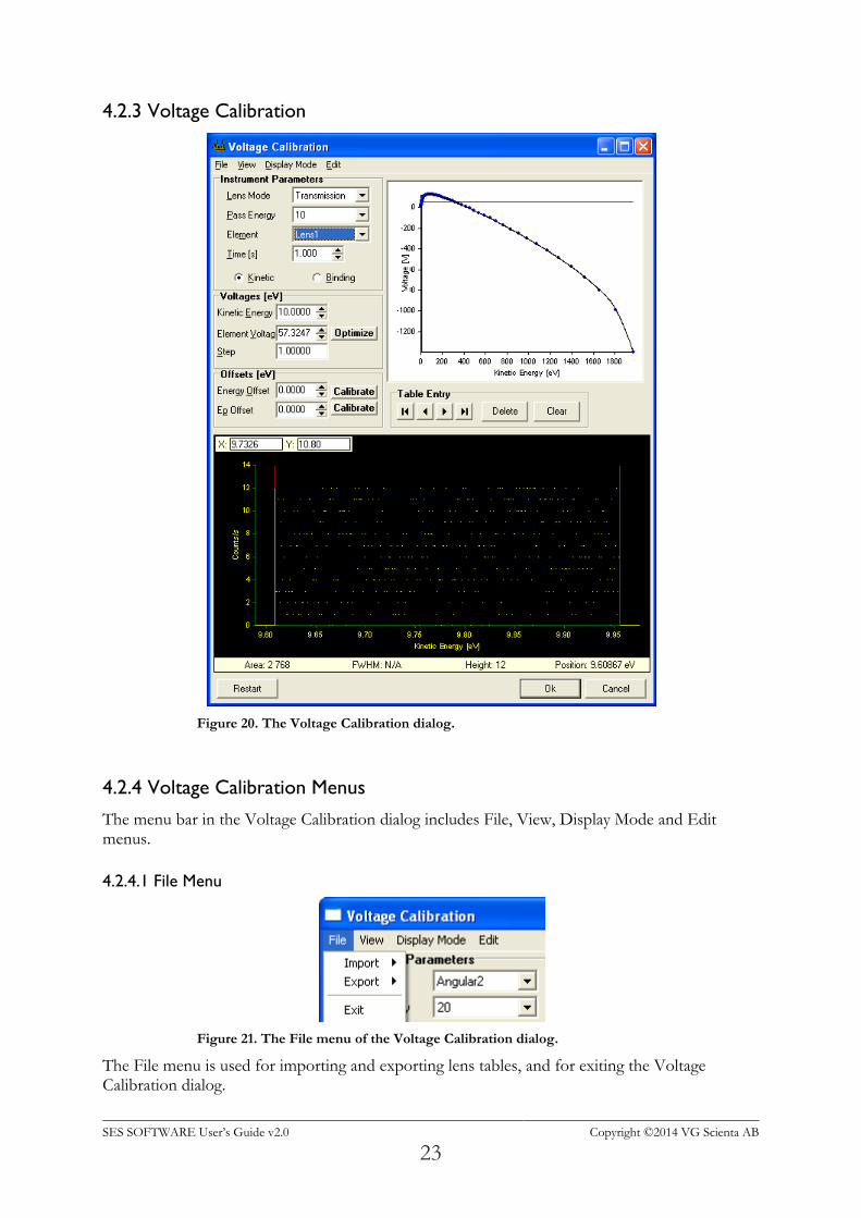
4.2.3 Voltage Calibration
Figure 20. The Voltage Calibration dialog.
4.2.4 Voltage Calibration Menus
The menu bar in the Voltage Calibration dialog includes File, View, Display Mode and Edit menus.
4.2.4.1 File Menu
Figure 21. The File menu of the Voltage Calibration dialog.
The File menu is used for importing and exporting lens tables, and for exiting the Voltage Calibration dialog.
SES SOFTWARE User’s Guide v2.0 Copyright ©2014 VG Scienta AB
24
Note: The user only has to use the Exit command in this menu. The remaining commands should only be used by the system administrator.
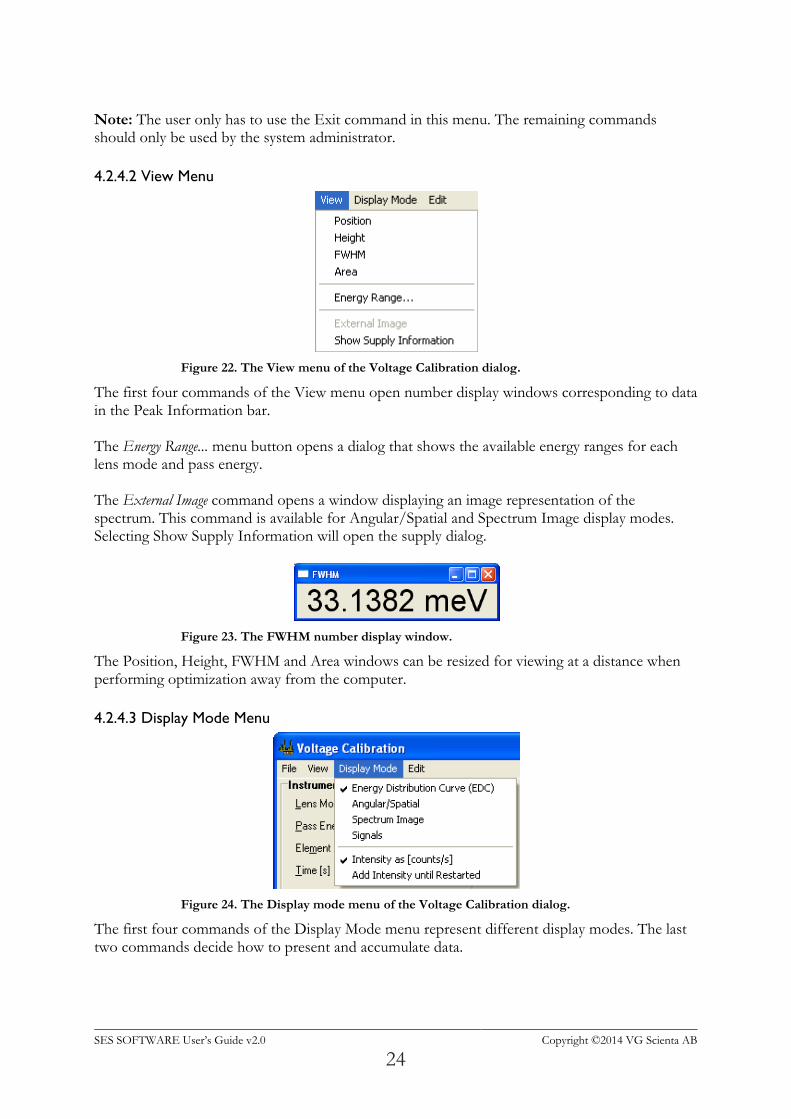
4.2.4.2 View Menu
Figure 22. The View menu of the Voltage Calibration dialog.
The first four commands of the View menu open number display windows corresponding to data in the Peak Information bar. The Energy Range... menu button opens a dialog that shows the available energy ranges for each lens mode and pass energy. The External Image command opens a window displaying an image representation of the spectrum. This command is available for Angular/Spatial and Spectrum Image display modes. Selecting Show Supply Information will open the supply dialog.
Figure 23. The FWHM number display window.
The Position, Height, FWHM and Area windows can be resized for viewing at a distance when performing optimization away from the computer.
4.2.4.3 Display Mode Menu
Figure 24. The Display mode menu of the Voltage Calibration dialog.
The first four commands of the Display Mode menu represent different display modes. The last two commands decide how to present and accumulate data.
SES SOFTWARE User’s Guide v2.0 Copyright ©2014 VG Scienta AB
25
Energy Distribution Curve
corresponds to a one-slice acquisition, presented as kinetic or binding energy vs. counts or count rate in the Spectrum Display.
Angular/Spatial
corresponds to an acquisition using the maximum number of slices available for current selection of Y Channels in the global detector settings. The data is summed over all Energy Channels, and then presented as Y channel vs. counts or count rate in the Spectrum Display.
Spectrum Image
corresponds to an acquisition using the maximum number of slices available for the current selection of Y Channels in the global detector settings. The data can be presented either as an image, or as kinetic or binding energy vs. counts or count rate for each slice individually, or summed over all slices. Note: The Spectrum Image item will have a submenu only if the detector system has a setting for Data Bytes.
Signals
If this command is checked, signal data will be displayed instead of spectrum data. If the Allow acquisition of both Signals and Detector option has been enabled in the SES Options dialog, both signal and spectrum data will be displayed simultaneously. Note: Signals are only available if an I/O interface library has been defined in the Instrument Installation dialog.
Intensity as [counts/s]
If this command is checked, the intensity of the acquired data will be displayed as count rate, rather than as counts.
Add Intensity until Restarted
If this command is checked, the intensity of subsequent acquisitions are added until either the Restart button is clicked, or changes made to the acquisition parameters forces the acquisition to restart.
4.2.4.4 Edit Menu
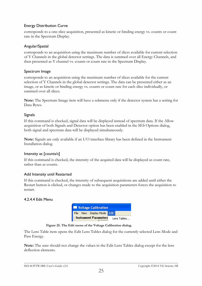
Figure 25. The Edit menu of the Voltage Calibration dialog.
The Lens Table item opens the Edit Lens Tables dialog for the currently selected Lens Mode and Pass Energy. Note: The user should not change the values in the Edit Lens Tables dialog except for the lens deflection elements.
SES SOFTWARE User’s Guide v2.0 Copyright ©2014 VG Scienta AB
26
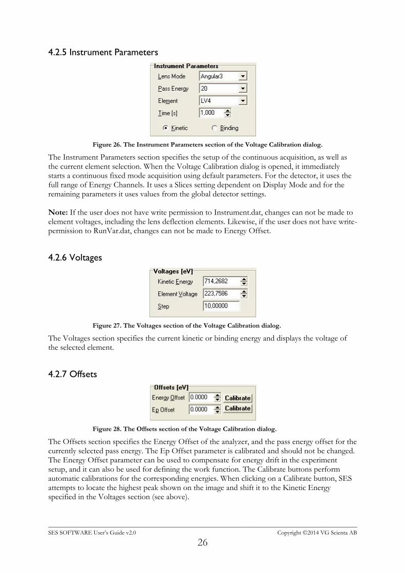
4.2.5 Instrument Parameters
Figure 26. The Instrument Parameters section of the Voltage Calibration dialog.
The Instrument Parameters section specifies the setup of the continuous acquisition, as well as the current element selection. When the Voltage Calibration dialog is opened, it immediately starts a continuous fixed mode acquisition using default parameters. For the detector, it uses the full range of Energy Channels. It uses a Slices setting dependent on Display Mode and for the remaining parameters it uses values from the global detector settings. Note: If the user does not have write permission to Instrument.dat, changes can not be made to element voltages, including the lens deflection elements. Likewise, if the user does not have write-permission to RunVar.dat, changes can not be made to Energy Offset.
4.2.6 Voltages
Figure 27. The Voltages section of the Voltage Calibration dialog.
The Voltages section specifies the current kinetic or binding energy and displays the voltage of the selected element.
4.2.7 Offsets
Figure 28. The Offsets section of the Voltage Calibration dialog.
The Offsets section specifies the Energy Offset of the analyzer, and the pass energy offset for the currently selected pass energy. The Ep Offset parameter is calibrated and should not be changed. The Energy Offset parameter can be used to compensate for energy drift in the experiment setup, and it can also be used for defining the work function. The Calibrate buttons perform automatic calibrations for the corresponding energies. When clicking on a Calibrate button, SES attempts to locate the highest peak shown on the image and shift it to the Kinetic Energy specified in the Voltages section (see above).
SES SOFTWARE User’s Guide v2.0 Copyright ©2014 VG Scienta AB
27
4.2.8 Lens Curve
The Lens Curve graph displays the lens table for the currently selected Element, if it depends on kinetic energy.
4.2.9 Table Entry
The Table Entry section provides means to navigate through the discrete kinetic energy/voltage pairs of the lens table for the currently selected element, if it depends on kinetic energy.
4.2.10 Spectrum Display
The spectrum display presents the spectrum of the current acquisition as a graph or as an image representation.
4.2.11 Signal Display
The signal display presents the signal data of the current acquisition.
4.2.12 Peak Information
The information displayed in the Peak Information Bar of the spectrum display can be used when maximizing intensity and resolution for desired analyzer settings.
4.3 How to Optimize the Lens Deflection Elements
4.3.1 Description
The two lens deflection elements called Up/Down and Left/Right can be used to optimize the sample position with regard to intensity or resolution.
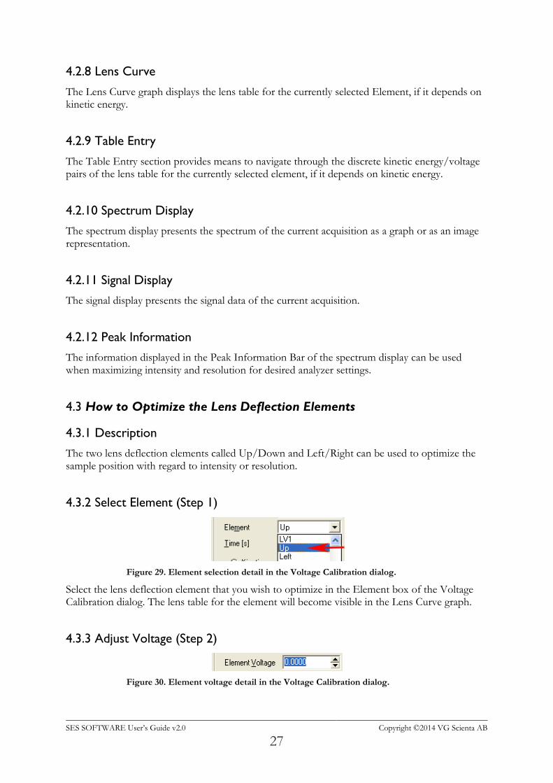
4.3.2 Select Element (Step 1)
Figure 29. Element selection detail in the Voltage Calibration dialog.
Select the lens deflection element that you wish to optimize in the Element box of the Voltage Calibration dialog. The lens table for the element will become visible in the Lens Curve graph.
4.3.3 Adjust Voltage (Step 2)
Figure 30. Element voltage detail in the Voltage Calibration dialog.
SES SOFTWARE User’s Guide v2.0 Copyright ©2014 VG Scienta AB
28
Next, use the Element Voltage box in the Voltage Calibration dialog to adjust the voltage for the lens deflection element while watching the Peak Information bar. Note: Changing settings related to the acquisition will force it to restart, and the Element Voltage for the lens deflection element will revert back to its initial value. Refer to the How to Edit the Lens Tables for instructions on how to save the new lens deflection voltages in the Lens Table.
4.3.4 Optimize (Step 3)
When optimizing for intensity, watch for an increase in peak height or spectrum area; when optimizing for energy resolution, watch for a decrease in peak FWHM, while maintaining good peak height. Note: Instrument operation is best when the lens deflection elements are at 0 V. It is better to optimize the intensity by changing experiment geometry.
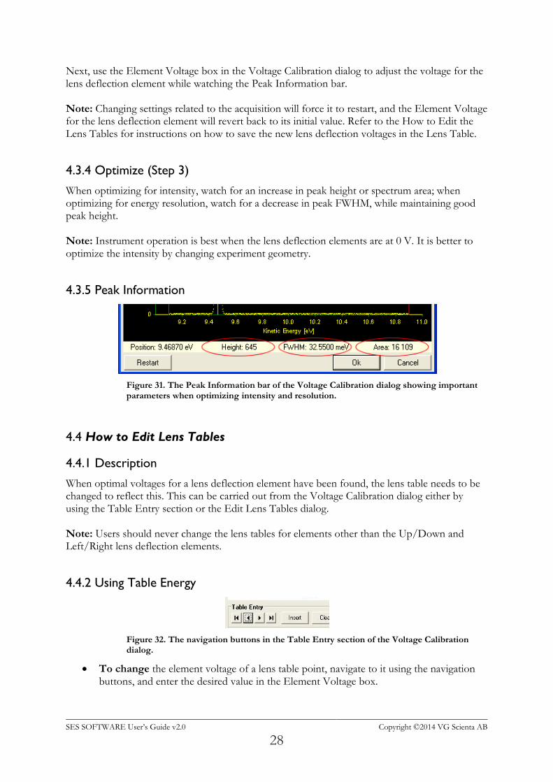
4.3.5 Peak Information
Figure 31. The Peak Information bar of the Voltage Calibration dialog showing important parameters when optimizing intensity and resolution.
4.4 How to Edit Lens Tables
4.4.1 Description
When optimal voltages for a lens deflection element have been found, the lens table needs to be changed to reflect this. This can be carried out from the Voltage Calibration dialog either by using the Table Entry section or the Edit Lens Tables dialog. Note: Users should never change the lens tables for elements other than the Up/Down and Left/Right lens deflection elements.
4.4.2 Using Table Energy
Figure 32. The navigation buttons in the Table Entry section of the Voltage Calibration dialog.
To change the element voltage of a lens table point, navigate to it using the navigation buttons, and enter the desired value in the Element Voltage box.
SES SOFTWARE User’s Guide v2.0 Copyright ©2014 VG Scienta AB
29
To delete a point, navigate to it and click the Delete button.
To insert a new point at the current kinetic energy, enter the desired value in Element Voltage and click the Insert button.
4.4.3 Using Edit Lens Table
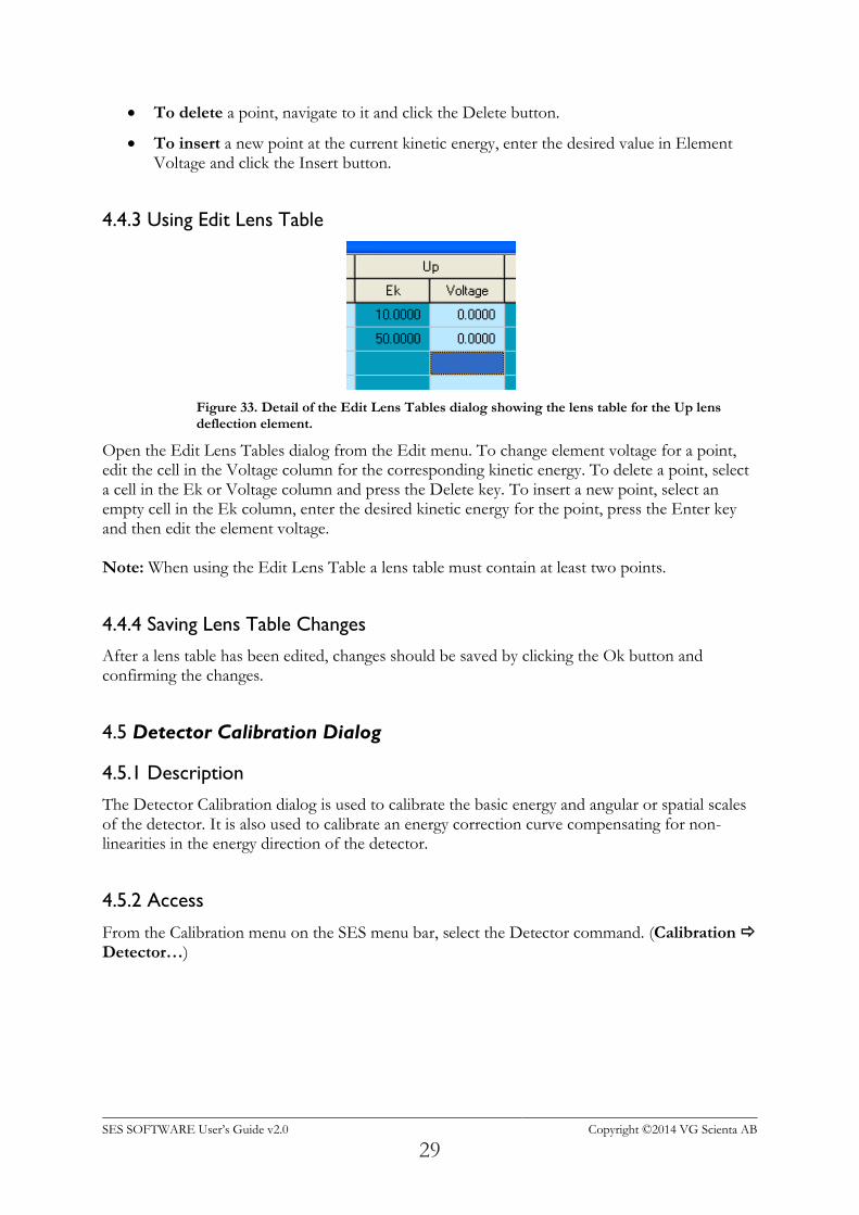
Figure 33. Detail of the Edit Lens Tables dialog showing the lens table for the Up lens deflection element.
Open the Edit Lens Tables dialog from the Edit menu. To change element voltage for a point, edit the cell in the Voltage column for the corresponding kinetic energy. To delete a point, select a cell in the Ek or Voltage column and press the Delete key. To insert a new point, select an empty cell in the Ek column, enter the desired kinetic energy for the point, press the Enter key and then edit the element voltage. Note: When using the Edit Lens Table a lens table must contain at least two points.
4.4.4 Saving Lens Table Changes
After a lens table has been edited, changes should be saved by clicking the Ok button and confirming the changes.
4.5 Detector Calibration Dialog
4.5.1 Description
The Detector Calibration dialog is used to calibrate the basic energy and angular or spatial scales of the detector. It is also used to calibrate an energy correction curve compensating for non-linearities in the energy direction of the detector.
4.5.2 Access
From the Calibration menu on the SES menu bar, select the Detector command. (Calibration Detector…)
SES SOFTWARE User’s Guide v2.0 Copyright ©2014 VG Scienta AB
30
4.5.3 Detector Calibration
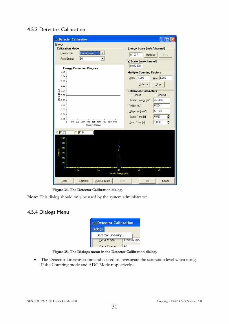
Figure 34. The Detector Calibration dialog.
Note: This dialog should only be used by the system administrator.
4.5.4 Dialogs Menu
Figure 35. The Dialogs menu in the Detector Calibration dialog.
The Detector Linearity command is used to investigate the saturation level when using Pulse Counting mode and ADC Mode respectively.
SES SOFTWARE User’s Guide v2.0 Copyright ©2014 VG Scienta AB
31
4.5.5 Calibration Mode
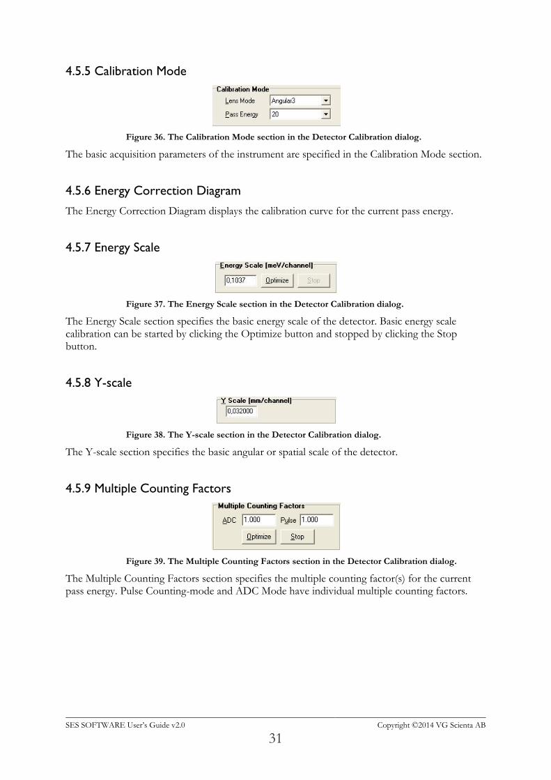
Figure 36. The Calibration Mode section in the Detector Calibration dialog.
The basic acquisition parameters of the instrument are specified in the Calibration Mode section.
4.5.6 Energy Correction Diagram
The Energy Correction Diagram displays the calibration curve for the current pass energy.
4.5.7 Energy Scale
Figure 37. The Energy Scale section in the Detector Calibration dialog.
The Energy Scale section specifies the basic energy scale of the detector. Basic energy scale calibration can be started by clicking the Optimize button and stopped by clicking the Stop button.
4.5.8 Y-scale
Figure 38. The Y-scale section in the Detector Calibration dialog.
The Y-scale section specifies the basic angular or spatial scale of the detector.
4.5.9 Multiple Counting Factors
Figure 39. The Multiple Counting Factors section in the Detector Calibration dialog.
The Multiple Counting Factors section specifies the multiple counting factor(s) for the current pass energy. Pulse Counting-mode and ADC Mode have individual multiple counting factors.
SES SOFTWARE User’s Guide v2.0 Copyright ©2014 VG Scienta AB
32
4.5.10 Calibration Parameters
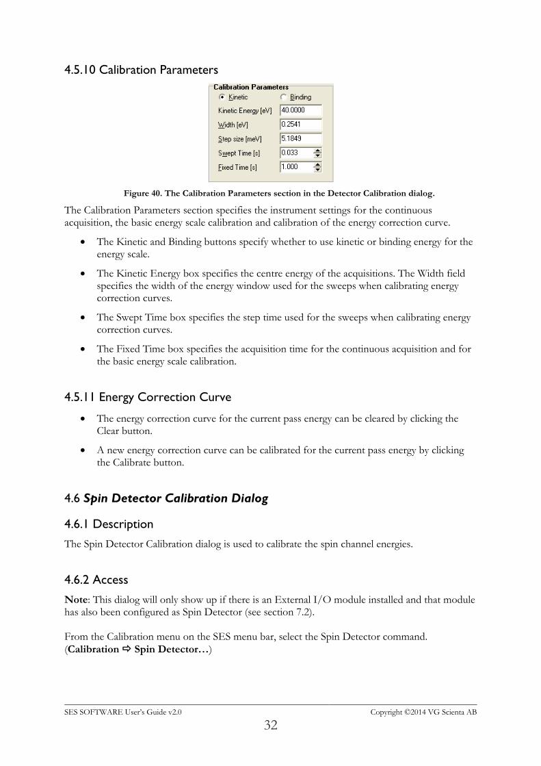
Figure 40. The Calibration Parameters section in the Detector Calibration dialog.
The Calibration Parameters section specifies the instrument settings for the continuous acquisition, the basic energy scale calibration and calibration of the energy correction curve.
The Kinetic and Binding buttons specify whether to use kinetic or binding energy for the energy scale.
The Kinetic Energy box specifies the centre energy of the acquisitions. The Width field specifies the width of the energy window used for the sweeps when calibrating energy correction curves.
The Swept Time box specifies the step time used for the sweeps when calibrating energy correction curves.
The Fixed Time box specifies the acquisition time for the continuous acquisition and for the basic energy scale calibration.
4.5.11 Energy Correction Curve
The energy correction curve for the current pass energy can be cleared by clicking the Clear button.
A new energy correction curve can be calibrated for the current pass energy by clicking the Calibrate button.
4.6 Spin Detector Calibration Dialog
4.6.1 Description
The Spin Detector Calibration dialog is used to calibrate the spin channel energies.
4.6.2 Access
Note: This dialog will only show up if there is an External I/O module installed and that module has also been configured as Spin Detector (see section 7.2). From the Calibration menu on the SES menu bar, select the Spin Detector command.
(Calibration Spin Detector…)
SES SOFTWARE User’s Guide v2.0 Copyright ©2014 VG Scienta AB
33
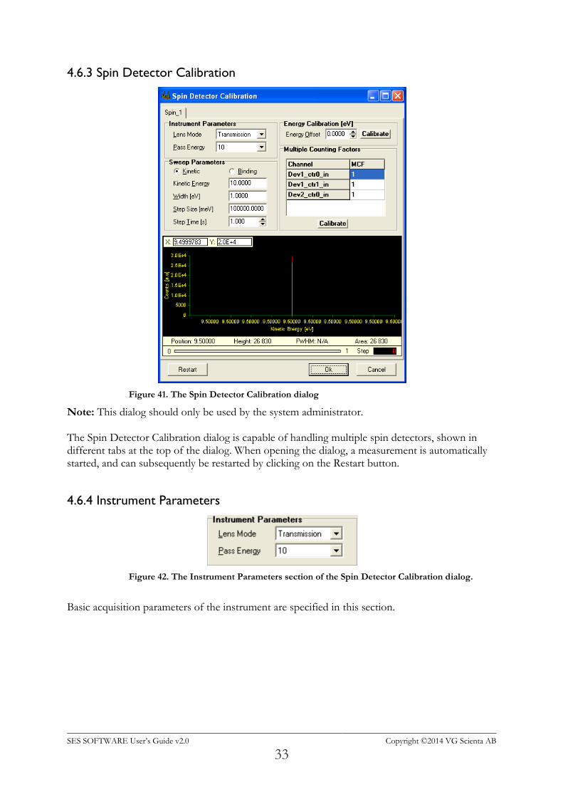
4.6.3 Spin Detector Calibration
Figure 41. The Spin Detector Calibration dialog
Note: This dialog should only be used by the system administrator. The Spin Detector Calibration dialog is capable of handling multiple spin detectors, shown in different tabs at the top of the dialog. When opening the dialog, a measurement is automatically started, and can subsequently be restarted by clicking on the Restart button.
4.6.4 Instrument Parameters
Figure 42. The Instrument Parameters section of the Spin Detector Calibration dialog.
Basic acquisition parameters of the instrument are specified in this section.
SES SOFTWARE User’s Guide v2.0 Copyright ©2014 VG Scienta AB
34
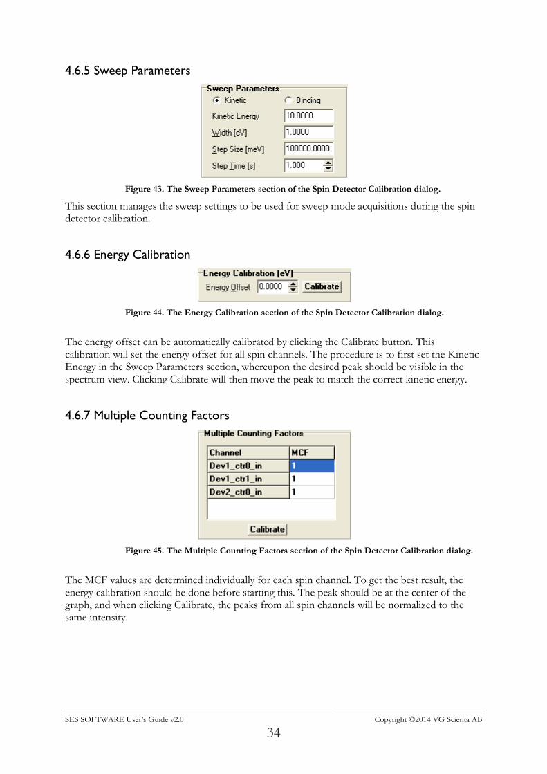
4.6.5 Sweep Parameters
Figure 43. The Sweep Parameters section of the Spin Detector Calibration dialog.
This section manages the sweep settings to be used for sweep mode acquisitions during the spin detector calibration.
4.6.6 Energy Calibration
Figure 44. The Energy Calibration section of the Spin Detector Calibration dialog.
The energy offset can be automatically calibrated by clicking the Calibrate button. This calibration will set the energy offset for all spin channels. The procedure is to first set the Kinetic Energy in the Sweep Parameters section, whereupon the desired peak should be visible in the spectrum view. Clicking Calibrate will then move the peak to match the correct kinetic energy.
4.6.7 Multiple Counting Factors
Figure 45. The Multiple Counting Factors section of the Spin Detector Calibration dialog.
The MCF values are determined individually for each spin channel. To get the best result, the energy calibration should be done before starting this. The peak should be at the center of the graph, and when clicking Calibrate, the peaks from all spin channels will be normalized to the same intensity.
SES SOFTWARE User’s Guide v2.0 Copyright ©2014 VG Scienta AB
35
4.7 Control Supplies Dialog
4.7.1 Description
The Control Supplies dialog is used to display and change the voltages assigned to specific supplies. It is used solely for troubleshooting the operation of the supplies.
4.7.2 Access
From the Calibration menu on the SES menu bar, select the Control Supplies command.
(Calibration Control Supplies…)
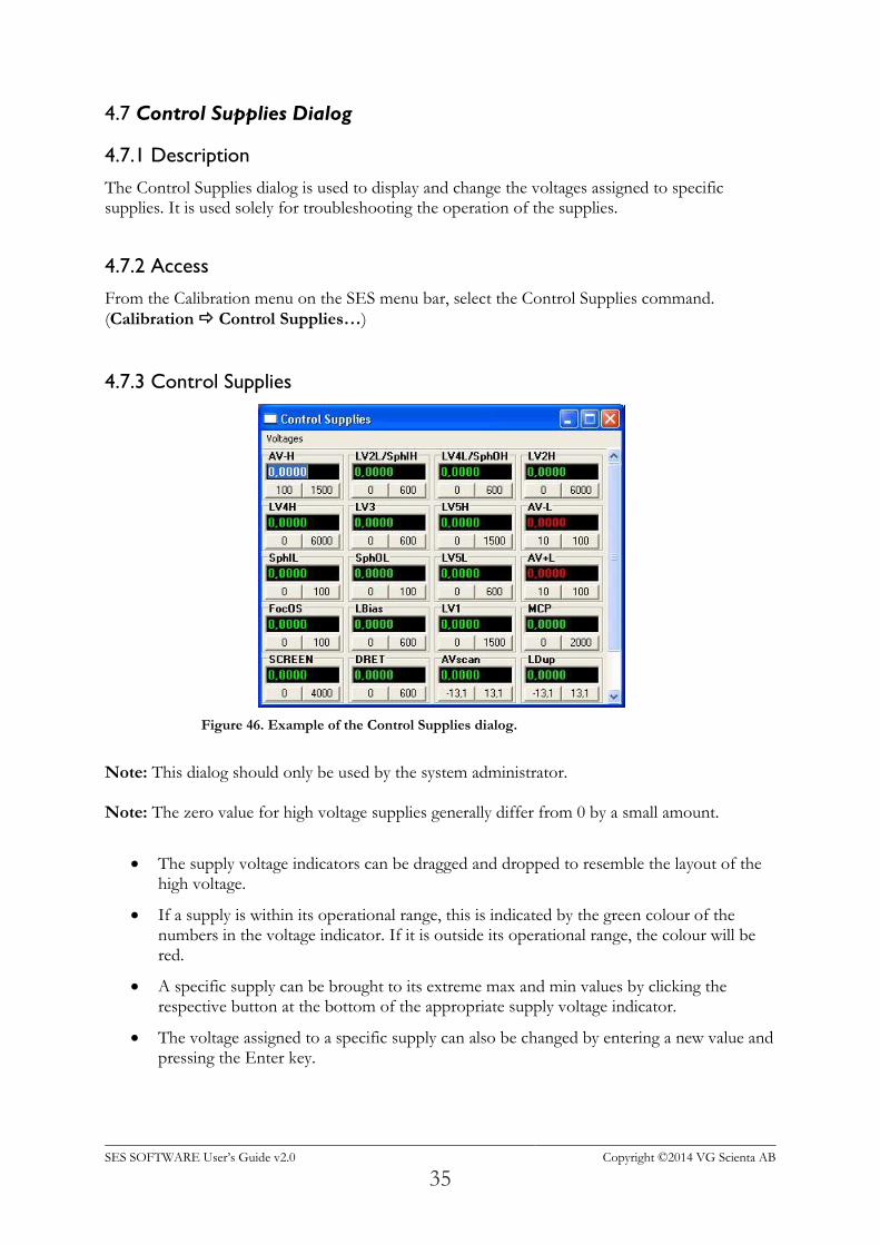
4.7.3 Control Supplies
Figure 46. Example of the Control Supplies dialog.
Note: This dialog should only be used by the system administrator. Note: The zero value for high voltage supplies generally differ from 0 by a small amount.
The supply voltage indicators can be dragged and dropped to resemble the layout of the high voltage.
If a supply is within its operational range, this is indicated by the green colour of the numbers in the voltage indicator. If it is outside its operational range, the colour will be red.
A specific supply can be brought to its extreme max and min values by clicking the respective button at the bottom of the appropriate supply voltage indicator.
The voltage assigned to a specific supply can also be changed by entering a new value and pressing the Enter key.
SES SOFTWARE User’s Guide v2.0 Copyright ©2014 VG Scienta AB
36
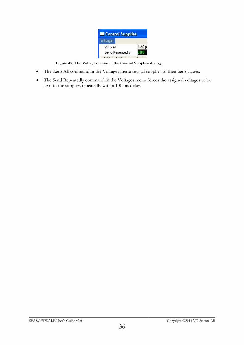
Figure 47. The Voltages menu of the Control Supplies dialog.
The Zero All command in the Voltages menu sets all supplies to their zero values.
The Send Repeatedly command in the Voltages menu forces the assigned voltages to be sent to the supplies repeatedly with a 100 ms delay.
SES SOFTWARE User’s Guide v2.0 Copyright ©2014 VG Scienta AB
37
5 SECTION E – Sequence Dialogs
5.1 Introduction
This section describes how to use the Sequence and Region Editors, explains the Run Modes, Special Regions and how to compensate for energy drifts during data acquisition.
5.2 Sequence List Editor
5.2.1 Desciption
The Sequence List Editor defines sequences to be run in an experiment batch. Each sequence in the sequence list uses individual settings.
5.2.2 Access
From the Sequence menu on the SES menu bar, select the Setup command. (Sequence Setup...) Note: The Sequence List Editor is only available if the Use Multiple Sequences option in the SES Options dialog is checked.
5.2.3 Sequence List Editor
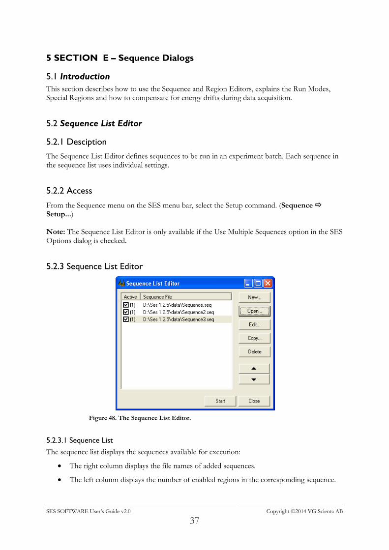
Figure 48. The Sequence List Editor.
5.2.3.1 Sequence List
The sequence list displays the sequences available for execution:
The right column displays the file names of added sequences.
The left column displays the number of enabled regions in the corresponding sequence.
SES SOFTWARE User’s Guide v2.0 Copyright ©2014 VG Scienta AB
38
5.2.3.2 Edit Buttons
The following buttons are available for editing the sequence list:
To create a new sequence, click the New… button. The new sequence is added to the end of the list.
To open one or more existing sequences, click the Open… button. The selected sequences are added to the end of the list.
To edit the selected sequence in the Sequence Editor Dialog, click the Edit… button.
To create a copy of a selected sequence, click the Copy… button.
To delete the selected sequence(s) from the list, click the Delete button.
To move the selected sequence(s) up or down in the queue, use the Up and Down buttons.
Note: Deleting a sequence from the sequence list does not delete the corresponding sequence file.
5.3 Sequence Editor
5.3.1 Description
The Sequence Editor defines the regions to be run in an experiment, which run mode to use and where to save resulting data.
5.3.2 Access
When using multiple sequences, double-click a sequence file or click the Edit button in the Sequence List Editor.
Otherwise, from the Sequence menu on the SES menu bar, select the Setup command.
(Sequence Setup…)
SES SOFTWARE User’s Guide v2.0 Copyright ©2014 VG Scienta AB
39
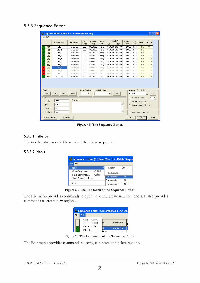
5.3.3 Sequence Editor
Figure 49. The Sequence Editor.
5.3.3.1 Title Bar
The title bar displays the file name of the active sequence.
5.3.3.2 Menu
Figure 50. The File menu of the Sequence Editor.
The File menu provides commands to open, save and create new sequences. It also provides commands to create new regions.
Figure 51. The Edit menu of the Sequence Editor.
The Edit menu provides commands to copy, cut, paste and delete regions.
SES SOFTWARE User’s Guide v2.0 Copyright ©2014 VG Scienta AB
40
5.3.3.3 Acquisition Region
The regions marked as active will be executed sequentially when an experiment is started.
To activate a region, click the centre of the cell of the first column so that it turns green
and the -symbol appears.
To deactivate a region, click the cell so that it turns red and the -symbol appears. Shaded columns are read only, and can be used to move regions up and down in the table. The second column of the region table defines the type of acquisition for the corresponding region:
D – acquisition using detector
r – acquisition using local detector settings
S – acquisition using signals
U – user interface region Note: The Total Time column displays the estimated time to complete one acquisition of the region. This includes the number of repetitions defined in the region in the calculation, but not analyzer delays.
5.3.3.4 Experiment Information
The Info section allows for miscellaneous experiment information to be entered including the base file name for saving experiment data.
5.3.3.5 Run Mode
The Run Mode section defines how the software should perform the acquisitions and save the data.
5.3.3.6 Buttons
To edit the global detector settings, click the Setup Detector button.
To edit the file options for this sequence, click the File Options button.
5.3.4 Saving Experiments
With the exception of the File Name box, all information entered in the Info section will be saved with the experiment. The text in the File Name box will be used as a base file name for the saved experiments.
If the Sort by User option is used, experiments will be saved in a subdirectory named as User.
If the Sort by Sample option is used, experiments will be saved in a subdirectory named as Sample.
If both Sort by User and Sort by Sample options are used, experiments will be saved in subdirectories of the form \User\Sample.
SES SOFTWARE User’s Guide v2.0 Copyright ©2014 VG Scienta AB
41
5.3.5 Region Management
The File and Edit menus contain commands for adding, editing, copying, and deleting regions. In addition, several shortcuts exist to speed up region management.
Create a new acquisition region (CTRL+R), through the Region command in the New submenu of the File menu, or click the New button.
Copy (CTRL+C), cut (CTRL+X), paste (CTRL+V) or delete (DEL) a region, select the corresponding row in the region table and click the appropriate command in the Edit menu or press, or click the corresponding button in the Region group.
To edit a region, double click the corresponding row in the region table to bring up the Region Editor, or edit the cells in the region table directly.
To move a region, click and hold on any of the read-only columns of the region table with the mouse, or hold the CTRL key and use the Up and Down keys.
5.4 Region Editor
5.4.1 Description
The Region Editor is used to define acquisition regions. The most basic settings for a region are lens mode, pass energy, and energy range. In addition to this, there are more advanced settings, such as using a region specific detector setting and run mode.
5.4.2 Access
In the Sequence Editor, double click a row in the region table.
SES SOFTWARE User’s Guide v2.0 Copyright ©2014 VG Scienta AB
42
5.4.3 Region Editor
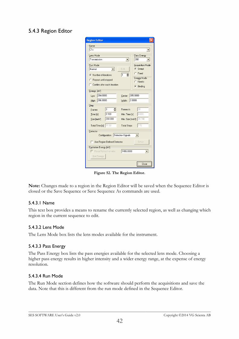
Figure 52. The Region Editor.
Note: Changes made to a region in the Region Editor will be saved when the Sequence Editor is closed or the Save Sequence or Save Sequence As commands are used.
5.4.3.1 Name
This text box provides a means to rename the currently selected region, as well as changing which region in the current sequence to edit.
5.4.3.2 Lens Mode
The Lens Mode box lists the lens modes available for the instrument.
5.4.3.3 Pass Energy
The Pass Energy box lists the pass energies available for the selected lens mode. Choosing a higher pass energy results in higher intensity and a wider energy range, at the expense of energy resolution.
5.4.3.4 Run Mode
The Run Mode section defines how the software should perform the acquisitions and save the data. Note that this is different from the run mode defined in the Sequence Editor.
SES SOFTWARE User’s Guide v2.0 Copyright ©2014 VG Scienta AB
43
5.4.3.5 Acquisition Mode
The Acquisition Mode section defines whether the region should be measured using fixed mode or swept mode. In fixed mode, the energy is kept fixed for the duration of the acquisition, so that a snapshot of the selected detector area is produced. The energy range is restricted by the energy width of the detector, which is typically about 10% of the pass energy. In swept mode, the energy is incremented by the energy step, starting with the low energy. Each step in energy corresponds to one point of the spectrum, and each step in energy is also integrated over the selected area of the detector.
5.4.3.6 Energy Mode
The Energy Mode section defines whether binding energy or kinetic energy should be used for defining the low and high energies and for the energy scale of the spectrum.
5.4.3.7 Energy
The Energy section defines the energy range of the region. It provides means of changing the energy range either by low and high energy, or by centre energy and energy width. The values in the Energy section are either in binding energy or kinetic energy, depending on the selected Energy Mode. If fixed acquisition mode is selected in Acquisition Mode, only the centre energy can be changed.
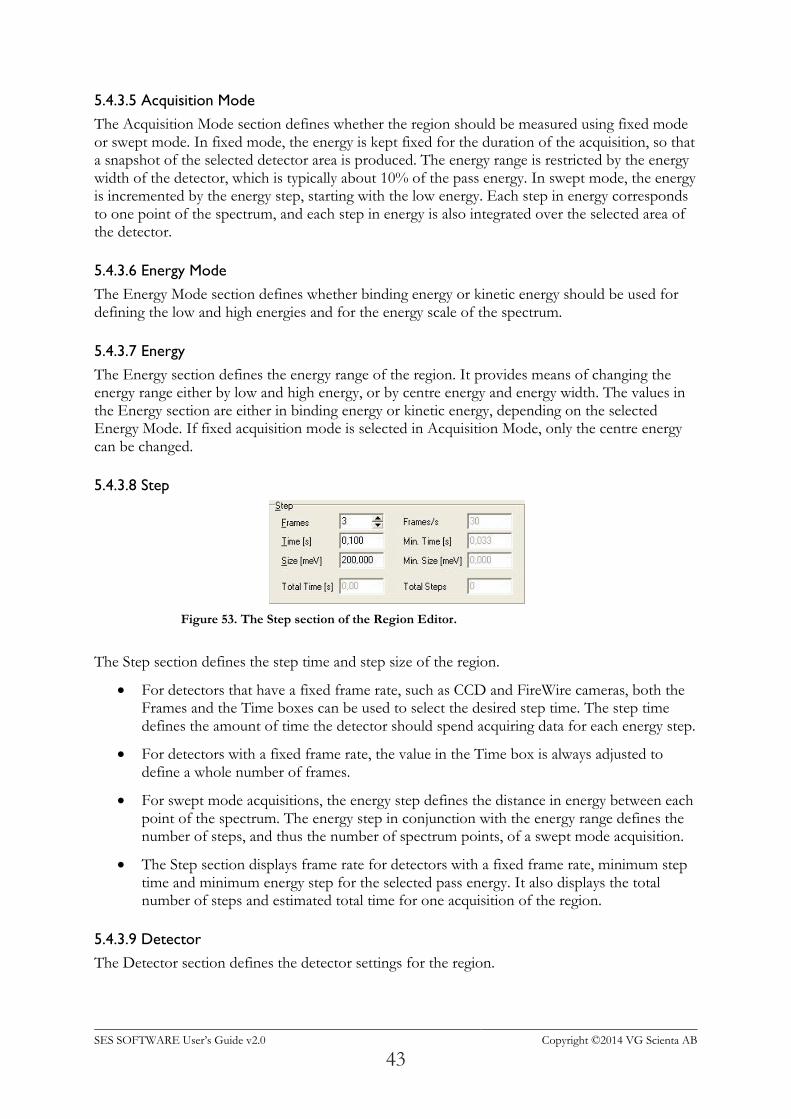
5.4.3.8 Step
Figure 53. The Step section of the Region Editor.
The Step section defines the step time and step size of the region.
For detectors that have a fixed frame rate, such as CCD and FireWire cameras, both the Frames and the Time boxes can be used to select the desired step time. The step time defines the amount of time the detector should spend acquiring data for each energy step.
For detectors with a fixed frame rate, the value in the Time box is always adjusted to define a whole number of frames.
For swept mode acquisitions, the energy step defines the distance in energy between each point of the spectrum. The energy step in conjunction with the energy range defines the number of steps, and thus the number of spectrum points, of a swept mode acquisition.
The Step section displays frame rate for detectors with a fixed frame rate, minimum step time and minimum energy step for the selected pass energy. It also displays the total number of steps and estimated total time for one acquisition of the region.
5.4.3.9 Detector
The Detector section defines the detector settings for the region.
SES SOFTWARE User’s Guide v2.0 Copyright ©2014 VG Scienta AB
44
The Configuration combo box determines if acquisition should be made through the detector and/or the Signals I/O.
If the Use Region Defined Detector box is unchecked, the region will use the global detector settings.
If the Use Region Defined Detector box is checked, it will use local detector settings specific to the region. The local detector settings can be changed by clicking the Setup button.
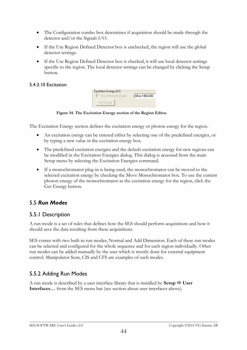
5.4.3.10 Excitation
Figure 54. The Excitation Energy section of the Region Editor.
The Excitation Energy section defines the excitation energy or photon energy for the region.
An excitation energy can be entered either by selecting one of the predefined energies, or by typing a new value in the excitation energy box.
The predefined excitation energies and the default excitation energy for new regions can be modified in the Excitation Energies dialog. This dialog is accessed from the main Setup menu by selecting the Excitation Energies command.
If a monochromator plug-in is being used, the monochromator can be moved to the selected excitation energy by checking the Move Monochromator box. To use the current photon energy of the monochromator as the excitation energy for the region, click the Get Energy button.
5.5 Run Modes
5.5.1 Description
A run mode is a set of rules that defines how the SES should perform acquisitions and how it should save the data resulting from these acquisitions. SES comes with two built-in run modes; Normal and Add Dimension. Each of these run modes can be selected and configured for the whole sequence and for each region individually. Other run modes can be added manually by the user which is mostly done for external equipment control. Manipulator Scan, CIS and CFS are examples of such modes.
5.5.2 Adding Run Modes
A run mode is described by a user interface library that is installed by Setup User Interfaces… from the SES menu bar (see section about user interfaces above).
SES SOFTWARE User’s Guide v2.0 Copyright ©2014 VG Scienta AB
45
5.5.3 Access
Run modes are selected and configured in the Run Mode sections of the Sequence Editor and the Region Editor for the sequence and regions respectively.
5.5.4 Global vs Local Run Modes
When the run mode is set in the Sequence Editor it is defined as Global, and when it is set for an individual region it is defined as Local. It is recommended to use multiple sequence files when handling more than one global run mode. The integrity of the region settings will be protected that way. All combinations of global and local run modes are not allowed for logical reasons. For example is it not possible to run a CIS region in a global CFS sequence, or a special manipulator region in a global manipulator scan sequence.
5.5.5 Normal and Add Dimension Run Modes
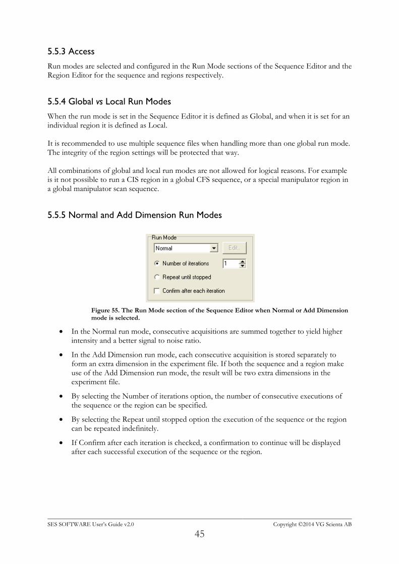
Figure 55. The Run Mode section of the Sequence Editor when Normal or Add Dimension mode is selected.
In the Normal run mode, consecutive acquisitions are summed together to yield higher intensity and a better signal to noise ratio.
In the Add Dimension run mode, each consecutive acquisition is stored separately to form an extra dimension in the experiment file. If both the sequence and a region make use of the Add Dimension run mode, the result will be two extra dimensions in the experiment file.
By selecting the Number of iterations option, the number of consecutive executions of the sequence or the region can be specified.
By selecting the Repeat until stopped option the execution of the sequence or the region can be repeated indefinitely.
If Confirm after each iteration is checked, a confirmation to continue will be displayed after each successful execution of the sequence or the region.
SES SOFTWARE User’s Guide v2.0 Copyright ©2014 VG Scienta AB
46
5.6 Special Regions
A special region is part of a user interface and becomes available when a user interface is installed
via Setup User Interfaces…. (analogous to run modes). In contradiction to normal regions, the action of a special region is not bound to spectrum acquisition. Mostly they control external equipment or signal input/output in a spectrometer system. Move Manipulator and Move Monochromator are examples of special regions (see sections below).
SES SOFTWARE User’s Guide v2.0 Copyright ©2014 VG Scienta AB
47
6 SECTION F – Operations during Acquisition
6.1 Introduction
This section describes the operations and information during data acquisition.
6.2 Operating the Spectrum Display
6.2.1 Description
The Spectrum Display is used to display acquired spectra, and can be configured to display data in several ways. During acquisition, it scales automatically to the acquired data, and it also has zooming capabilities and can display basic peak information.
6.2.2 Spectrum Display
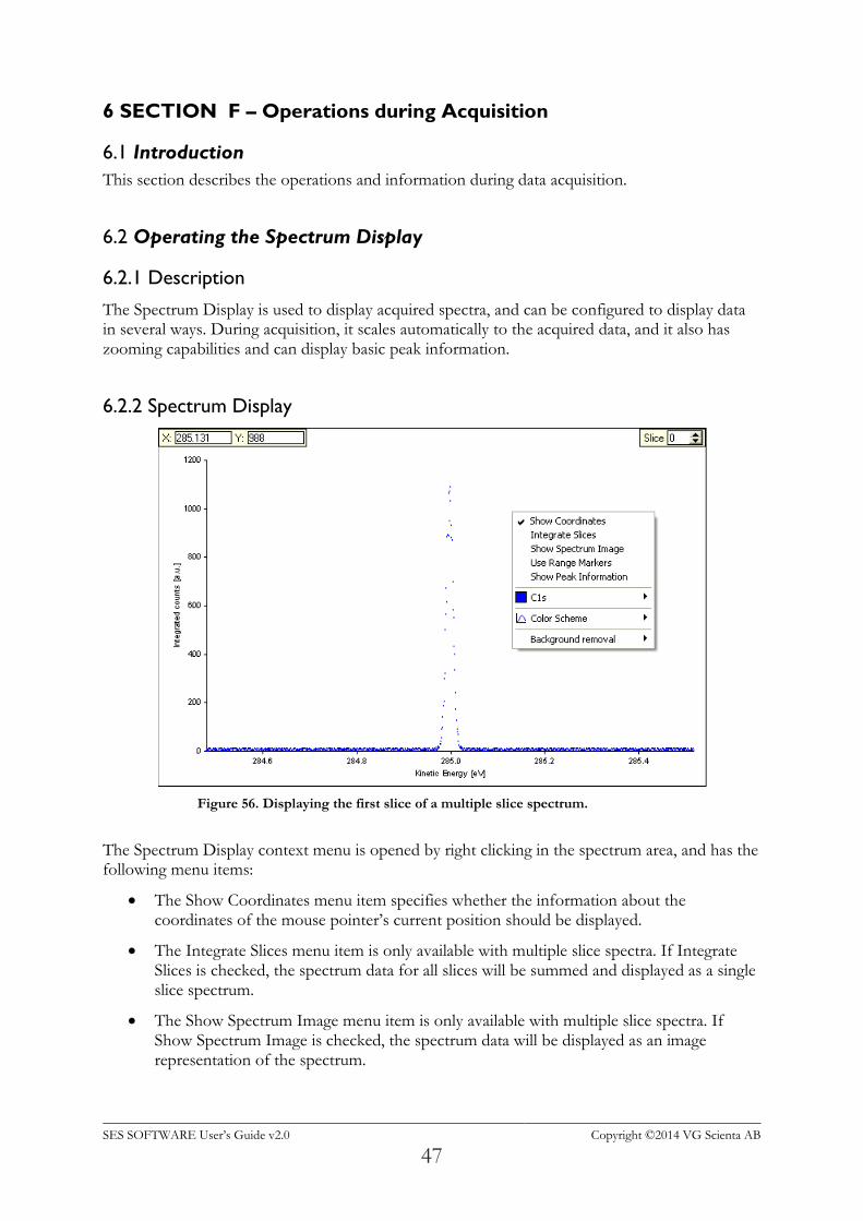
Figure 56. Displaying the first slice of a multiple slice spectrum.
The Spectrum Display context menu is opened by right clicking in the spectrum area, and has the following menu items:
The Show Coordinates menu item specifies whether the information about the coordinates of the mouse pointer’s current position should be displayed.
The Integrate Slices menu item is only available with multiple slice spectra. If Integrate Slices is checked, the spectrum data for all slices will be summed and displayed as a single slice spectrum.
The Show Spectrum Image menu item is only available with multiple slice spectra. If Show Spectrum Image is checked, the spectrum data will be displayed as an image representation of the spectrum.
SES SOFTWARE User’s Guide v2.0 Copyright ©2014 VG Scienta AB
48
The Use Range Markers menu item specifies whether only data within the area of the range markers should be displayed.
The Show Peak Information menu item specifies whether basic peak information should be displayed at the bottom of the spectrum display.
The C1s menu item is named after the region that is being displayed, and is only visible if the spectrum has as a graph. Its sub menu specifies whether the graph should be drawn using lines or points as well as the colour of the graph. The sub menu also allows more detailed modification of the curve by opening a Customize dialog.
The Colour Scheme item specifies what colours to use for the background of the spectrum display, as well as for the axes and the text. When selecting a colour scheme, the colour of the graph will be reset to the default value for that colour scheme.
Note: The Integrate Slices and Show Spectrum Image commands are mutually exclusive. By checking either one of them, the other will automatically be unchecked. If either one of them is checked the Slice box will not be visible.
6.2.3 Customize Curve Dialog
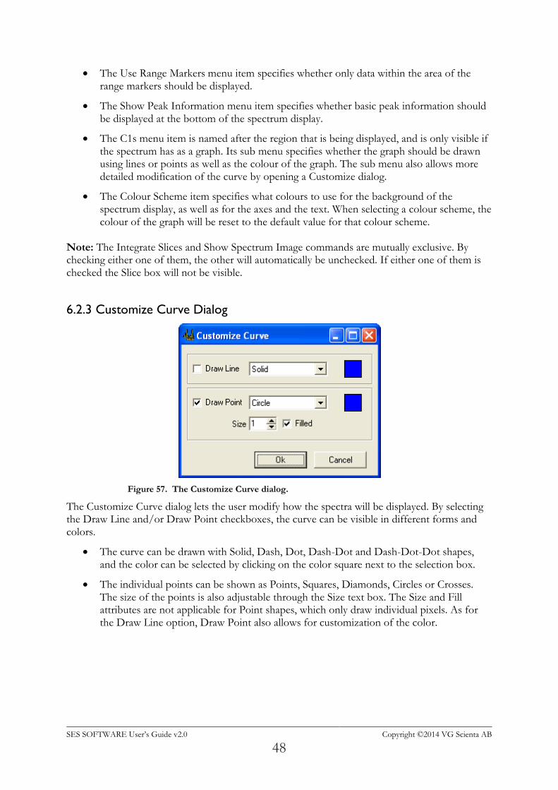
Figure 57. The Customize Curve dialog.
The Customize Curve dialog lets the user modify how the spectra will be displayed. By selecting the Draw Line and/or Draw Point checkboxes, the curve can be visible in different forms and colors.
The curve can be drawn with Solid, Dash, Dot, Dash-Dot and Dash-Dot-Dot shapes, and the color can be selected by clicking on the color square next to the selection box.
The individual points can be shown as Points, Squares, Diamonds, Circles or Crosses. The size of the points is also adjustable through the Size text box. The Size and Fill attributes are not applicable for Point shapes, which only draw individual pixels. As for the Draw Line option, Draw Point also allows for customization of the color.
SES SOFTWARE User’s Guide v2.0 Copyright ©2014 VG Scienta AB
49
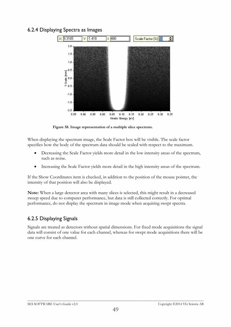
6.2.4 Displaying Spectra as Images
Figure 58. Image representation of a multiple slice spectrum.
When displaying the spectrum image, the Scale Factor box will be visible. The scale factor specifies how the body of the spectrum data should be scaled with respect to the maximum.
Decreasing the Scale Factor yields more detail in the low intensity areas of the spectrum, such as noise.
Increasing the Scale Factor yields more detail in the high intensity areas of the spectrum. If the Show Coordinates item is checked, in addition to the position of the mouse pointer, the intensity of that position will also be displayed. Note: When a large detector area with many slices is selected, this might result in a decreased sweep speed due to computer performance, but data is still collected correctly. For optimal performance, do not display the spectrum in image mode when acquiring swept spectra.
6.2.5 Displaying Signals
Signals are treated as detectors without spatial dimensions. For fixed mode acquisitions the signal data will consist of one value for each channel, whereas for swept mode acquisitions there will be one curve for each channel.
SES SOFTWARE User’s Guide v2.0 Copyright ©2014 VG Scienta AB
50
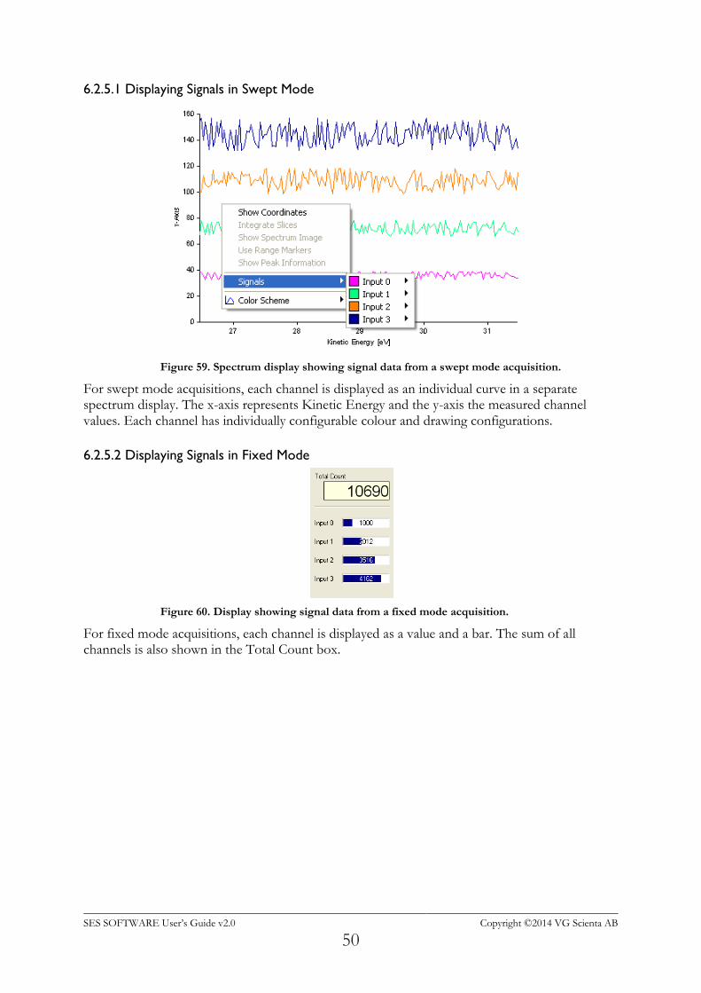
6.2.5.1 Displaying Signals in Swept Mode
Figure 59. Spectrum display showing signal data from a swept mode acquisition.
For swept mode acquisitions, each channel is displayed as an individual curve in a separate spectrum display. The x-axis represents Kinetic Energy and the y-axis the measured channel values. Each channel has individually configurable colour and drawing configurations.
6.2.5.2 Displaying Signals in Fixed Mode
Figure 60. Display showing signal data from a fixed mode acquisition.
For fixed mode acquisitions, each channel is displayed as a value and a bar. The sum of all channels is also shown in the Total Count box.
SES SOFTWARE User’s Guide v2.0 Copyright ©2014 VG Scienta AB
51
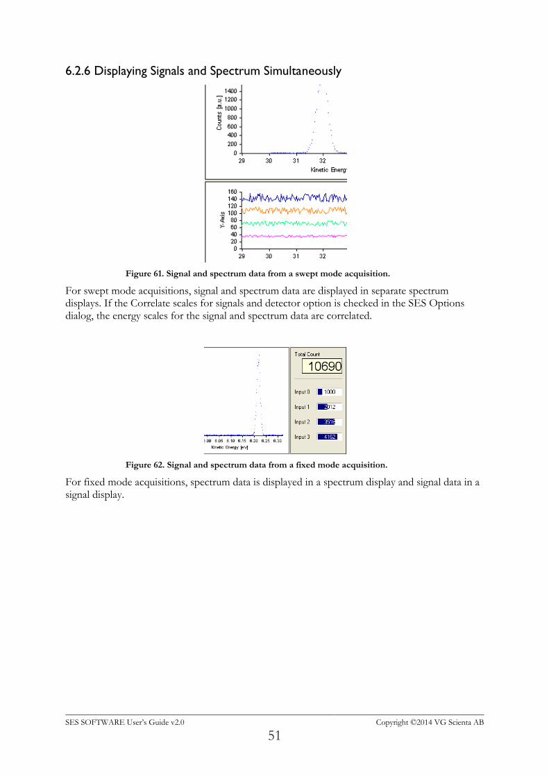
6.2.6 Displaying Signals and Spectrum Simultaneously
Figure 61. Signal and spectrum data from a swept mode acquisition.
For swept mode acquisitions, signal and spectrum data are displayed in separate spectrum displays. If the Correlate scales for signals and detector option is checked in the SES Options dialog, the energy scales for the signal and spectrum data are correlated.
Figure 62. Signal and spectrum data from a fixed mode acquisition.
For fixed mode acquisitions, spectrum data is displayed in a spectrum display and signal data in a signal display.
SES SOFTWARE User’s Guide v2.0 Copyright ©2014 VG Scienta AB
52
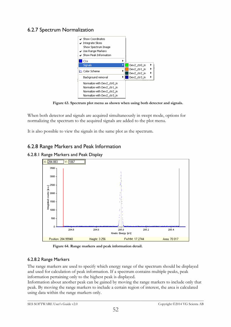
6.2.7 Spectrum Normalization
Figure 63. Spectrum plot menu as shown when using both detector and signals.
When both detector and signals are acquired simultaneously in swept mode, options for normalizing the spectrum to the acquired signals are added to the plot menu. It is also possible to view the signals in the same plot as the spectrum.
6.2.8 Range Markers and Peak Information
6.2.8.1 Range Markers and Peak Display
Figure 64. Range markers and peak information detail.
6.2.8.2 Range Markers
The range markers are used to specify which energy range of the spectrum should be displayed and used for calculation of peak information. If a spectrum contains multiple peaks, peak information pertaining only to the highest peak is displayed. Information about another peak can be gained by moving the range markers to include only that peak. By moving the range markers to include a certain region of interest, the area is calculated using data within the range markers only.
SES SOFTWARE User’s Guide v2.0 Copyright ©2014 VG Scienta AB
53
6.2.8.3 Peak Information
The Peak Information bar displays information pertaining to the highest peak in the spectrum.
Position describes the energy position of the highest point.
Height describes the intensity of the highest point.
FWHM describes the full width at half maximum of the peak.
Area describes the total intensity over the whole spectrum.
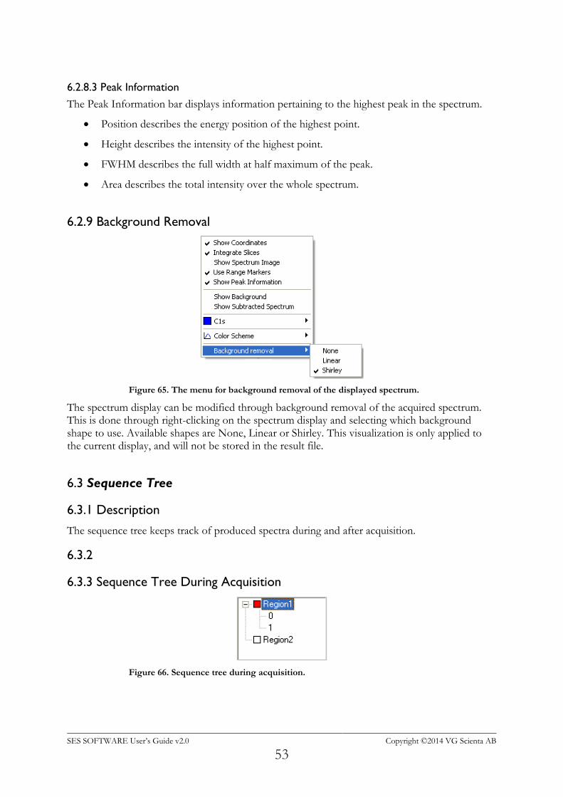
6.2.9 Background Removal
Figure 65. The menu for background removal of the displayed spectrum.
The spectrum display can be modified through background removal of the acquired spectrum. This is done through right-clicking on the spectrum display and selecting which background shape to use. Available shapes are None, Linear or Shirley. This visualization is only applied to the current display, and will not be stored in the result file.
6.3 Sequence Tree
6.3.1 Description
The sequence tree keeps track of produced spectra during and after acquisition.
6.3.2
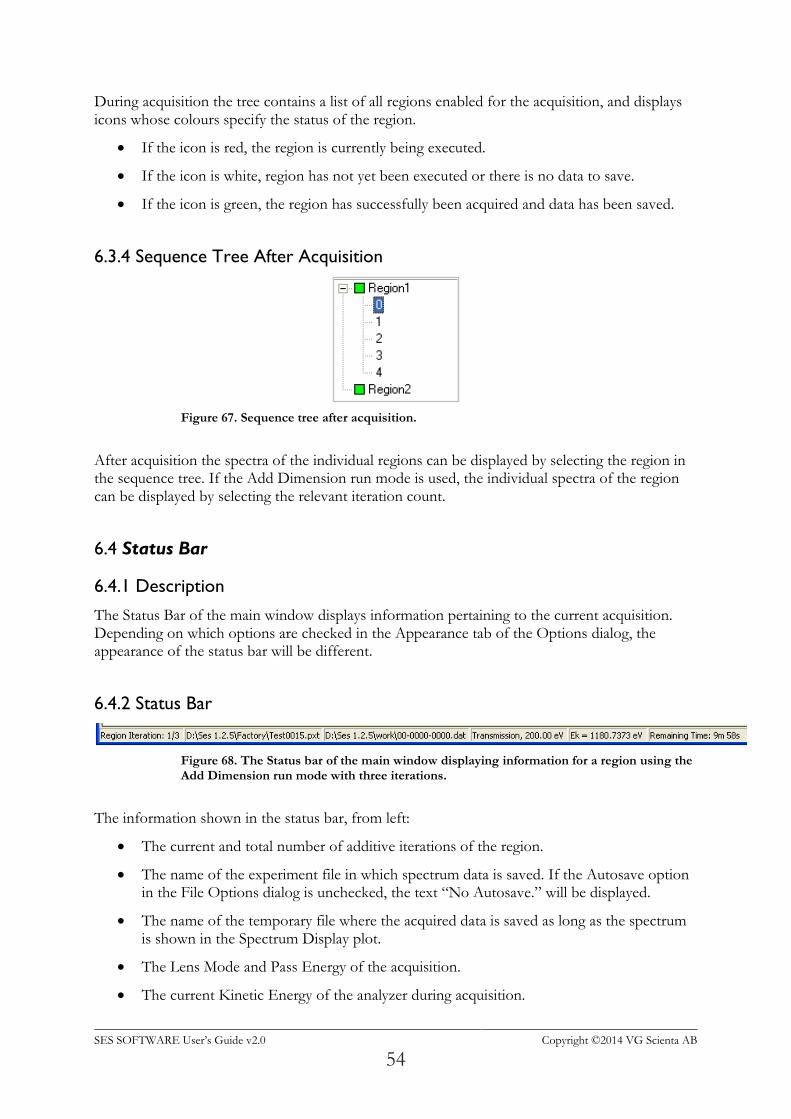
6.3.3 Sequence Tree During Acquisition
Figure 66. Sequence tree during acquisition.
SES SOFTWARE User’s Guide v2.0 Copyright ©2014 VG Scienta AB
54
During acquisition the tree contains a list of all regions enabled for the acquisition, and displays icons whose colours specify the status of the region.
If the icon is red, the region is currently being executed.
If the icon is white, region has not yet been executed or there is no data to save.
If the icon is green, the region has successfully been acquired and data has been saved.
6.3.4 Sequence Tree After Acquisition
Figure 67. Sequence tree after acquisition.
After acquisition the spectra of the individual regions can be displayed by selecting the region in the sequence tree. If the Add Dimension run mode is used, the individual spectra of the region can be displayed by selecting the relevant iteration count.
6.4 Status Bar
6.4.1 Description
The Status Bar of the main window displays information pertaining to the current acquisition. Depending on which options are checked in the Appearance tab of the Options dialog, the appearance of the status bar will be different.
6.4.2 Status Bar
Figure 68. The Status bar of the main window displaying information for a region using the Add Dimension run mode with three iterations.
The information shown in the status bar, from left:
The current and total number of additive iterations of the region.
The name of the experiment file in which spectrum data is saved. If the Autosave option in the File Options dialog is unchecked, the text “No Autosave.” will be displayed.
The name of the temporary file where the acquired data is saved as long as the spectrum is shown in the Spectrum Display plot.
The Lens Mode and Pass Energy of the acquisition.
The current Kinetic Energy of the analyzer during acquisition.
SES SOFTWARE User’s Guide v2.0 Copyright ©2014 VG Scienta AB
55
The estimated remaining time of the acquisition.
SES SOFTWARE User’s Guide v2.0 Copyright ©2014 VG Scienta AB
56
7 SECTION G – Installations Dialogs
7.1 Introduction
This section describes the installation dialogs that are used for the initial setup of a new system.
7.2 Instrument Installation Dialog
7.2.1 Description
The Instrument Installation dialog is used to change basic settings of the instrument, such as which detector and supply libraries to use.
7.2.2 Access
From the Installation menu on the SES menu bar, select the Instrument command. (Installation
Instrument...)
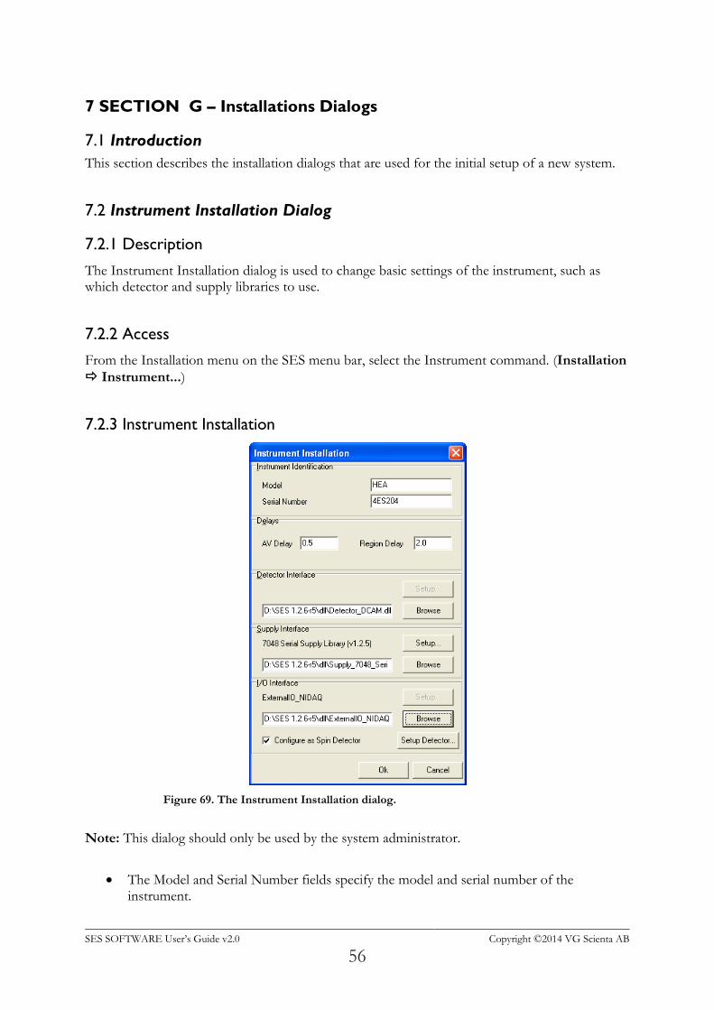
7.2.3 Instrument Installation
Figure 69. The Instrument Installation dialog.
Note: This dialog should only be used by the system administrator.
The Model and Serial Number fields specify the model and serial number of the instrument.
SES SOFTWARE User’s Guide v2.0 Copyright ©2014 VG Scienta AB
57
The AV Delay specifies the delay used when the voltage of a high voltage supply is changed. The Region Delay specifies the delay used between the regions in a sequence.
The Detector Interface section specifies which detector library to use for data acquisition. To change library, click the Browse button and to change library settings, click the Setup button.
The Supply Interface section specifies which supply library to use to control the HV supplies. To change library, click the Browse button and to change library settings, click the Setup button.
The I/O Interface section specifies which I/O library to use for external I/O communication. To change library, click the Browse button and to change library settings, click the Setup button.
The Configure as Spin Detector check-box enables the External I/O interface to be used specifically for spin detectors.
Note: Shipped with SES come dummy libraries for each interface. They are named Detector_Dummy.dll, Supply_Dummy.dll and ExternalIO_NIDAQ_Dummy.dll respectively.
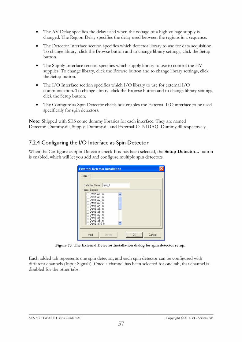
7.2.4 Configuring the I/O Interface as Spin Detector
When the Configure as Spin Detector check-box has been selected, the Setup Detector... button is enabled, which will let you add and configure multiple spin detectors.
Figure 70. The External Detector Installation dialog for spin detector setup.
Each added tab represents one spin detector, and each spin detector can be configured with different channels (Input Signals). Once a channel has been selected for one tab, that channel is disabled for the other tabs.
SES SOFTWARE User’s Guide v2.0 Copyright ©2014 VG Scienta AB
58
7.3 Supply Installation Dialog
7.3.1 Description
The Supply Installation dialog is used to add and remove supplies, and to change their settings and calibration parameters.
7.3.2 Access
From the Installation menu on the SES menu bar, select the Supplies command. (Installation Supplies…)
7.3.3 Supply Installation
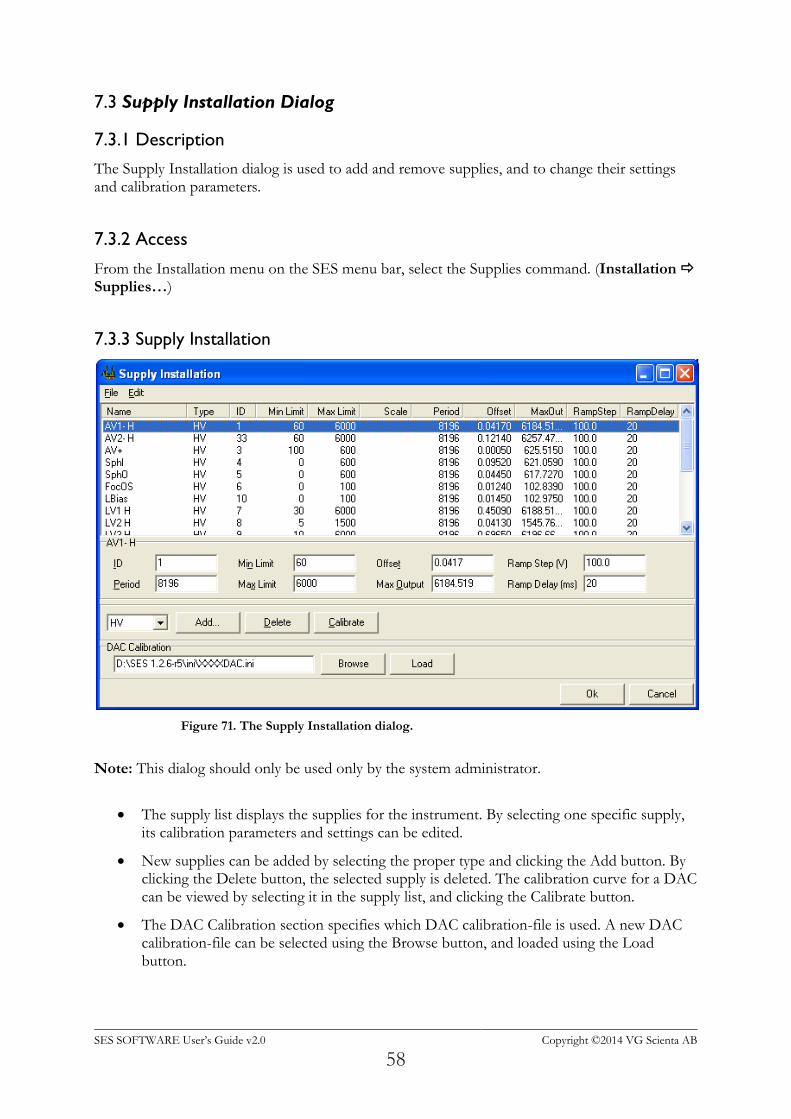
Figure 71. The Supply Installation dialog.
Note: This dialog should only be used only by the system administrator.
The supply list displays the supplies for the instrument. By selecting one specific supply, its calibration parameters and settings can be edited.
New supplies can be added by selecting the proper type and clicking the Add button. By clicking the Delete button, the selected supply is deleted. The calibration curve for a DAC can be viewed by selecting it in the supply list, and clicking the Calibrate button.
The DAC Calibration section specifies which DAC calibration-file is used. A new DAC calibration-file can be selected using the Browse button, and loaded using the Load button.
SES SOFTWARE User’s Guide v2.0 Copyright ©2014 VG Scienta AB
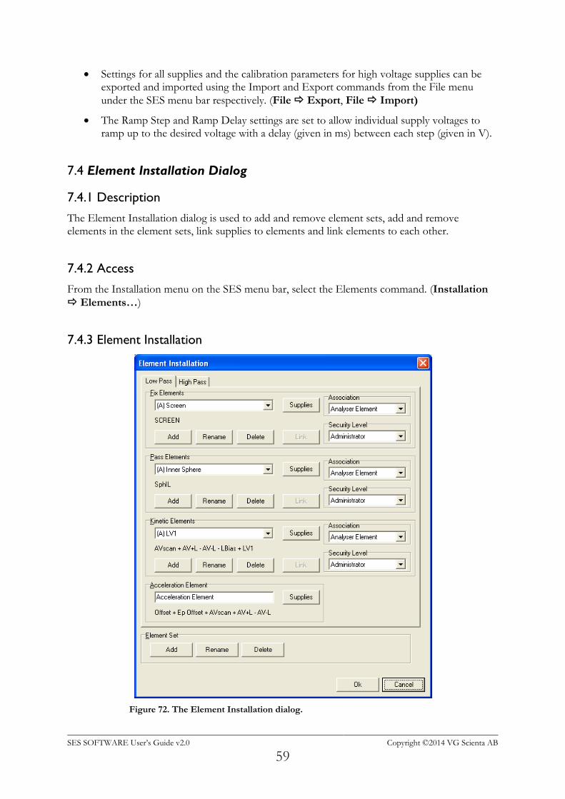
59
Settings for all supplies and the calibration parameters for high voltage supplies can be exported and imported using the Import and Export commands from the File menu
under the SES menu bar respectively. (File Export, File Import)
The Ramp Step and Ramp Delay settings are set to allow individual supply voltages to ramp up to the desired voltage with a delay (given in ms) between each step (given in V).
7.4 Element Installation Dialog
7.4.1 Description
The Element Installation dialog is used to add and remove element sets, add and remove elements in the element sets, link supplies to elements and link elements to each other.
7.4.2 Access
From the Installation menu on the SES menu bar, select the Elements command. (Installation
Elements…)
7.4.3 Element Installation
Figure 72. The Element Installation dialog.
SES SOFTWARE User’s Guide v2.0 Copyright ©2014 VG Scienta AB
60
Note: This dialog should only be used only by the system administrator.
The tabs specify the different element sets available to the instrument.
The Fix Elements section defines elements which are neither dependent on pass energy nor kinetic energy.
The Pass Elements section defines elements which are dependent on pass energy, but not kinetic energy.
The Kinetic Elements section defines elements which are dependent on both pass energy and kinetic energy.
Acceleration Element section defines the acceleration element.
7.4.4 Modifying Elements and Element Sets
Elements in all the different sections described above can be:
Added by clicking the Add button.
Deleted or renamed by clicking the Delete or Rename buttons.
Linked to an element further up in the list by clicking the Link button.
The supplies linked to an element can be changed by clicking the Supplies button.
The association for an element can be changed using the Assosiations drop-down list. Available values are Analyzer Element, Detector Element or External I/O Element.
The security level for an element can be changed using the Security Level drop-down list. Available values are Administrator, Privileged User and User, where Administrator is the highest level.
Element sets can be added, deleted or renamed by clicking the corresponding buttons in the Element Sets section.
Note: Associations are important when using an instrument which has both signals and a detector, and where elements associated with each input interface should be turned off when that interface is not used.
7.5 Lens Mode Installation Dialog
7.5.1 Description
The Lens Mode dialog is used to add and remove lens modes and to add and remove pass energies.
7.5.2 Access
From the Installation menu on the SES menu bar, select the Lens Modes command.
(Installation Lens Modes...)
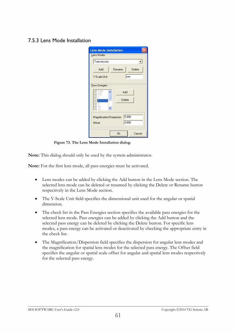
SES SOFTWARE User’s Guide v2.0 Copyright ©2014 VG Scienta AB
61
7.5.3 Lens Mode Installation
Figure 73. The Lens Mode Installation dialog.
Note: This dialog should only be used by the system administrator. Note: For the first lens mode, all pass energies must be activated.
Lens modes can be added by clicking the Add button in the Lens Mode section. The selected lens mode can be deleted or renamed by clicking the Delete or Rename button respectively in the Lens Mode section.
The Y-Scale Unit field specifies the dimensional unit used for the angular or spatial dimension.
The check list in the Pass Energies section specifies the available pass energies for the selected lens mode. Pass energies can be added by clicking the Add button and the selected pass energy can be deleted by clicking the Delete button. For specific lens modes, a pass energy can be activated or deactivated by checking the appropriate entry in the check list.
The Magnification/Dispersion field specifies the dispersion for angular lens modes and the magnification for spatial lens modes for the selected pass energy. The Offset field specifies the angular or spatial scale offset for angular and spatial lens modes respectively for the selected pass energy.
SES SOFTWARE User’s Guide v2.0 Copyright ©2014 VG Scienta AB
62
7.6 Application Examples
7.6.1 Installing a New HV Supply
In addition to installation of a new HV supply in the rack, the supply has to be defined in the SES software. The following steps should be performed:
1. Identify a free optical output (marked with a plain numeric ID) on the DOM board in the rack. Make a note of the ID number.
2. Start SES and add a new supply in the Supply Installation dialog. Select “HV” from the drop-down menu. Enter the selected ID number.
3. Read the A and B calibration parameters that are printed on the HV Supply hardware and enter them into the Supply Installation dialog. A is the Offset value in mV B is the Max Output value in V Note: Offset and Max Output are both given in Volts in SES.
4. Enter the other parameters for the supply. Period, Ramp Step and Ramp Delay can be copied from other supplies but Max Lim and Min Lim are unique for the new supply since they define the operating voltage range.
5. Close the dialog and save the data by clicking the Save button when asked to.
6. Install the HV supply in the rack and connect it with a fibre to the selected optical output of the DOM board.
7.6.2 Installing a New DAC Board
In addition to installation of a new DAC board in the rack, the DAC has to be defined in the SES software. The following steps should be performed:
1. Identify a free optical output (marked with the letter “D” and a numeric ID) on the DOM board in the rack. Make a note of the ID.
2. Set the 8-bit dip switch on the DAC board to the selected ID number in binary format. Switch 1-8 correspond to bits 0-7, and the ON state corresponds to a logical “1”. For example: ON, OFF, ON, OFF, OFF, OFF, OFF, OFF corresponds to 00000101 which represents ID = 5.
3. Check that a DAC calibration data file is available for the new DAC.
4. Start SES and add a new DAC in the Supply Installation dialog. Select “DAC20” from the drop down menu. Enter the selected ID.
5. Enter the other parameters for the DAC. They can all be copied from other DAC boards in the list.
6. Make a note of the path and file name of the current DAC.ini file that is stated in the bottom of the dialog.
SES SOFTWARE User’s Guide v2.0 Copyright ©2014 VG Scienta AB
63
7. Close the dialog and save the data by clicking the Save button when asked to.
8. Exit SES and open the DAC ini file as well as the new DAC calibration data file. Copy the new calibration data into the DAC ini file and save it
9. Install the new DAC in the rack and connect it with a fibre to the selected optical output of the DOM board.
7.6.3 Double HV Rack Configurations
A DOM (Digital Output Module) board in a HV rack is able to address 16 DAC cards and 32 HV supplies. If this is not enough, additional DOM boards have to be installed, either in the same rack or in additional racks that share the same serial communication line to the PC. Each DOM board is given a base address plus a 5 bit address space. This space of 32 addresses (i.e. board ID numbers) can be used for DAC’s as well as HV supplies since these two types of boards are controlled by two different command types from SES. Hence, there is no conflict addressing a DAC and a HV supply with identical ID’s. The DOM board has a four bit jumper area where the base address of the board is programmed. This jumper area corresponds to the high nibble of the board ID in SES. The first DOM board with base address 0 should have jumper setting 0000. The second one at base address 32 should have 0010. The third one at base address 64 should have 0100 and so on (0 means jumper present and 1 means jumper removed).
7.6.4 Extra Acceleration Voltage Chain
In some cases, such as spin detector applications, a large number of HV cards on the detector side have to be biased on the Hertzog (i.e. acceleration) voltage. In order to reduce the load on the accelerating chain supplies, and to minimize the risk for crosstalk between the analyzer and the detector parts, a copy of the accelerating chain can be installed in parallel to the real Hertzog voltage. The following steps should be performed in order to install two HV supplies that bias the spin detector to the same potential as the Hertzog plate.
1. Add two HV supplies to the rack and configure the spin detector filterbox in a way that the spin detector is biased to the sum of the supplies (that are denoted SAV- and SAV + in this text). The voltage ranges and polarities should be selected to match the specific analyzer energy range. These operations are part of production and service work at VG Scienta and should not be performed by normal SES users.
2. Define the HV supplies in SES according to previous section.
3. Open the Element Installation dialog and add a new “Kinetic” element (named SAV in this example).
4. Inspect the Accelerating chain supply configuration in the dialog and associate the same set of supplies to the SAV element but with opposite sign. Then add SAV+ and SAV- supplies to the SAV association list. For example: If the Accelerating element has the following configuration: Offset + Ep Offset + AVScan + (AV+) – (AV-)
SES SOFTWARE User’s Guide v2.0 Copyright ©2014 VG Scienta AB
64
SAV should have following configuration: - AVScan - (AV+) + (AV-) + (SAV+) – (SAV-)
Close the dialog and save the data by clicking the Save button when asked to.
5. Open the lens table editor from the Calibration Voltage dialog. The table for SAV should be just two entries long. Enter (0, 0) and (Max, 0) where Max stands for the highest kinetic energy that will be measured. The settings above makes SAV to act as a virtual element at zero Volts, forcing the SAV supply chain voltage to be equal to the Hertzog chain voltage.
6. Create identical tables for all pass energies that you will use. Close the dialog and save the data by clicking the Save button when asked to.
7. Turn on the HV rack and play with the pass energies and kinetic energies using the Voltage Calibration dialog. Check that the voltage supply settings behave as predicted in the Supply Information window.
8. Measure with a high voltage probe and a multimeter on the filter box electrodes and confirm that the Hertzog voltage and the SAV voltage follow each other. Note: No DAC board is included in the SAV chain in this example which means that the voltage steps of SAV becomes larger than the steps of the real Hertzog voltage.
7.6.5 Kinetic Energy Output as a Voltage
In some cases, add-on equipment to the analyzer needs information about the measured kinetic energy in real time. This can be communicated as an analog voltage from the HV rack. In the following example a DAC is employed for generation of a voltage that is proportional to the measured kinetic energy, but a HV Supply could be used as well. Only the calibration routines differ.
1. Install a new DAC in the rack and define it in SES according to previous section.
2. Restart SES and define a new “Kinetic” element in the Element Installation dialog and associate it to the new DAC via the corresponding Supplies button.
3. Open the lens table editor from the Calibration Voltage dialog and enter the table for the new DAC. It should contain just two entries representing a straight line between (0, 0) and (Max Ek, Max V) where Max V is the voltage that should be output at a certain kinetic energy Max Ek. For example: If 5V output should correspond to Ek = 1keV, the table should have the following entries: (0, 0), (1000, 5). This type of table makes the DAC output proportional to the measured kinetic energy but other relations can easily be implemented by just extending the table.
4. Create identical tables for all pass energies that you will use. Close the dialog and save the data by clicking the Save button when asked to.
5. Turn on the HV rack and play with the pass energies and kinetic energies using the Voltage Calibration dialog. Check that the DAC setting behave as predicted in the Supply Information window.
SES SOFTWARE User’s Guide v2.0 Copyright ©2014 VG Scienta AB
65
6. Measure the DAC output with a multimeter and confirm that the voltage is proportional to the kinetic energy as required.
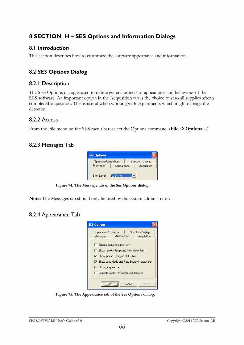
SES SOFTWARE User’s Guide v2.0 Copyright ©2014 VG Scienta AB
66
8 SECTION H – SES Options and Information Dialogs
8.1 Introduction
This section describes how to customize the software appearance and information.
8.2 SES Options Dialog
8.2.1 Description
The SES Options dialog is used to define general aspects of appearance and behaviour of the SES software. An important option in the Acquisition tab is the choice to zero all supplies after a completed acquisition. This is useful when working with experiments which might damage the detector.
8.2.2 Access
From the File menu on the SES menu bar, select the Options command. (File Options…)
8.2.3 Messages Tab
Figure 74. The Message tab of the Ses Options dialog.
Note: The Messages tab should only be used by the system administrator.
8.2.4 Appearance Tab
Figure 75. The Appearance tab of the Ses Options dialog.
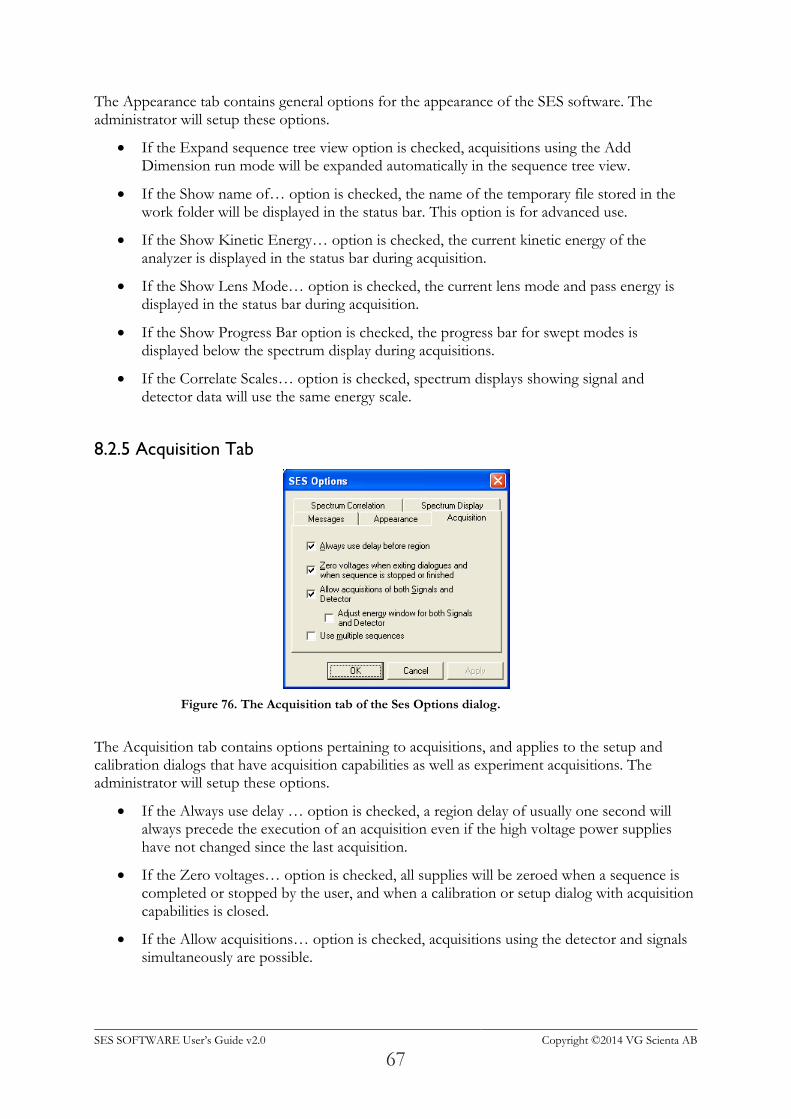
SES SOFTWARE User’s Guide v2.0 Copyright ©2014 VG Scienta AB
67
The Appearance tab contains general options for the appearance of the SES software. The administrator will setup these options.
If the Expand sequence tree view option is checked, acquisitions using the Add Dimension run mode will be expanded automatically in the sequence tree view.
If the Show name of… option is checked, the name of the temporary file stored in the work folder will be displayed in the status bar. This option is for advanced use.
If the Show Kinetic Energy… option is checked, the current kinetic energy of the analyzer is displayed in the status bar during acquisition.
If the Show Lens Mode… option is checked, the current lens mode and pass energy is displayed in the status bar during acquisition.
If the Show Progress Bar option is checked, the progress bar for swept modes is displayed below the spectrum display during acquisitions.
If the Correlate Scales… option is checked, spectrum displays showing signal and detector data will use the same energy scale.
8.2.5 Acquisition Tab
Figure 76. The Acquisition tab of the Ses Options dialog.
The Acquisition tab contains options pertaining to acquisitions, and applies to the setup and calibration dialogs that have acquisition capabilities as well as experiment acquisitions. The administrator will setup these options.
If the Always use delay … option is checked, a region delay of usually one second will always precede the execution of an acquisition even if the high voltage power supplies have not changed since the last acquisition.
If the Zero voltages… option is checked, all supplies will be zeroed when a sequence is completed or stopped by the user, and when a calibration or setup dialog with acquisition capabilities is closed.
If the Allow acquisitions… option is checked, acquisitions using the detector and signals simultaneously are possible.
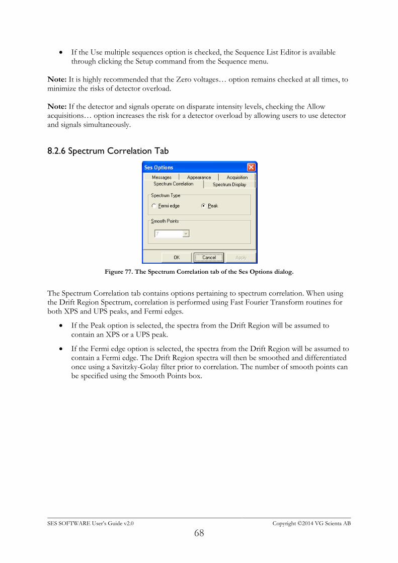
SES SOFTWARE User’s Guide v2.0 Copyright ©2014 VG Scienta AB
68
If the Use multiple sequences option is checked, the Sequence List Editor is available through clicking the Setup command from the Sequence menu.
Note: It is highly recommended that the Zero voltages… option remains checked at all times, to minimize the risks of detector overload. Note: If the detector and signals operate on disparate intensity levels, checking the Allow acquisitions… option increases the risk for a detector overload by allowing users to use detector and signals simultaneously.
8.2.6 Spectrum Correlation Tab
Figure 77. The Spectrum Correlation tab of the Ses Options dialog.
The Spectrum Correlation tab contains options pertaining to spectrum correlation. When using the Drift Region Spectrum, correlation is performed using Fast Fourier Transform routines for both XPS and UPS peaks, and Fermi edges.
If the Peak option is selected, the spectra from the Drift Region will be assumed to contain an XPS or a UPS peak.
If the Fermi edge option is selected, the spectra from the Drift Region will be assumed to contain a Fermi edge. The Drift Region spectra will then be smoothed and differentiated once using a Savitzky-Golay filter prior to correlation. The number of smooth points can be specified using the Smooth Points box.
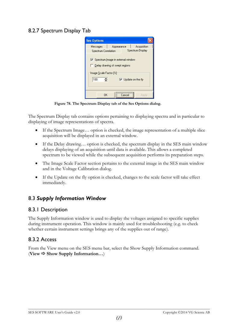
SES SOFTWARE User’s Guide v2.0 Copyright ©2014 VG Scienta AB
69
8.2.7 Spectrum Display Tab
Figure 78. The Spectrum Display tab of the Ses Options dialog.
The Spectrum Display tab contains options pertaining to displaying spectra and in particular to displaying of image representations of spectra.
If the Spectrum Image… option is checked, the image representation of a multiple slice acquisition will be displayed in an external window.
If the Delay drawing… option is checked, the spectrum display in the SES main window delays displaying of an acquisition until data is available. This allows a completed spectrum to be viewed while the subsequent acquisition performs its preparation steps.
The Image Scale Factor section pertains to the external image in the SES main window and in the Voltage Calibration dialog.
If the Update on the fly option is checked, changes to the scale factor will take effect immediately.
8.3 Supply Information Window
8.3.1 Description
The Supply Information window is used to display the voltages assigned to specific supplies during instrument operation. This window is mainly used for troubleshooting (e.g. to check whether certain instrument settings brings any of the supplies out of range).
8.3.2 Access
From the View menu on the SES menu bar, select the Show Supply Information command.
(View Show Supply Information…)
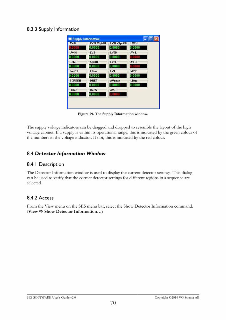
SES SOFTWARE User’s Guide v2.0 Copyright ©2014 VG Scienta AB
70
8.3.3 Supply Information
Figure 79. The Supply Information window.
The supply voltage indicators can be dragged and dropped to resemble the layout of the high voltage cabinet. If a supply is within its operational range, this is indicated by the green colour of the numbers in the voltage indicator. If not, this is indicated by the red colour.
8.4 Detector Information Window
8.4.1 Description
The Detector Information window is used to display the current detector settings. This dialog can be used to verify that the correct detector settings for different regions in a sequence are selected.
8.4.2 Access
From the View menu on the SES menu bar, select the Show Detector Information command.
(View Show Detector Information…)
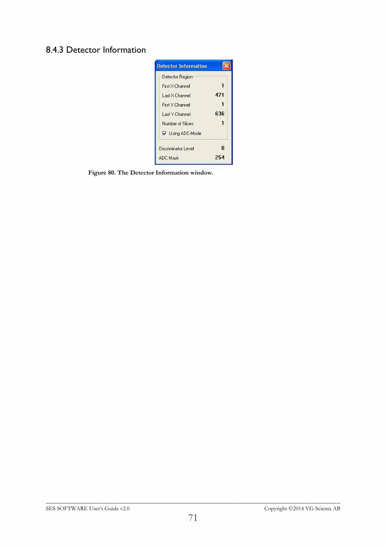
SES SOFTWARE User’s Guide v2.0 Copyright ©2014 VG Scienta AB
71
8.4.3 Detector Information
Figure 80. The Detector Information window.
SES SOFTWARE User’s Guide v2.0 Copyright ©2014 VG Scienta AB
72
9 SECTION I – Manipulator
9.1 Introduction
This section describes how to operate a manipulator user interface in SES, how to install the software and how to test the functionality. Manipulator control requires a general manipulator library but also a hardware dependent plug-in library. All examples are given for the McLennan SimStep stepper motor controllers but the principles apply to all brands of controllers.
9.2 Installation
9.2.1 Connecting the Controller
The PC should be connected to the manipulator controller hardware prior to software installation. The SimStep stepper controllers operate through a standard RS232 protocol, and in this case the controller should be connected via a serial (COM) port. Other controllers employ GPIB, Ethernet, or USB for example.
9.2.2 Adding the General Manipulator Library
The general manipulator library is installed by adding the Manipulator.dll in the list of user
interfaces under Setup User Interfaces… from the SES menu bar (see section about user interfaces above). Once the Manipulator.dll library has been added to the list, the Manipulator menu appears on the SES menu bar.
9.2.3 Adding the Hardware Dependent Plug-in Library
While the general manipulator library is a control library for all types of manipulators, the hardware dependent plug-in handles the communication with specific hardware. The following steps should be taken to install the ManiHW_SimStep.dll library for the SimStep controllers.
1. Select the Manipulator.dll file and click the Setup... button in the User Interfaces dialog,
or select Manipulator Setup… from the SES menu bar. The Setup Manipulator dialog is opened by both actions.
2. Click the Browse button and select the ManiHW_SimStep.dll library. The dialog is shown below.
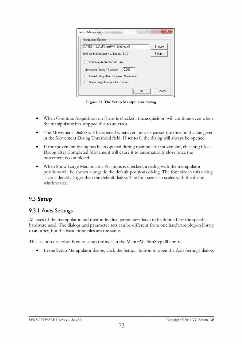
SES SOFTWARE User’s Guide v2.0 Copyright ©2014 VG Scienta AB
73
Figure 81. The Setup Manipulator dialog.
When Continue Acquisition on Error is checked, the acquisition will continue even when the manipulator has stopped due to an error.
The Movement Dialog will be opened whenever any axis passes the threshold value given in the Movement Dialog Threshold field. If set to 0, the dialog will always be opened.
If the movement dialog has been opened during manipulator movement, checking Close Dialog after Completed Movement will cause it to automatically close once the movement is completed.
When Show Large Manipulator Positions is checked, a dialog with the manipulator positions will be shown alongside the default positions dialog. The font size in this dialog is considerably larger than the default dialog. The font size also scales with the dialog window size.
9.3 Setup
9.3.1 Axes Settings
All axes of the manipulator and their individual parameters have to be defined for the specific hardware used. The dialogs and parameter sets can be different from one hardware plug-in library to another, but the basic principles are the same. This section describes how to setup the axes in the ManiHW_SimStep.dll library.
In the Setup Manipulator dialog, click the Setup... button to open the Axis Settings dialog.
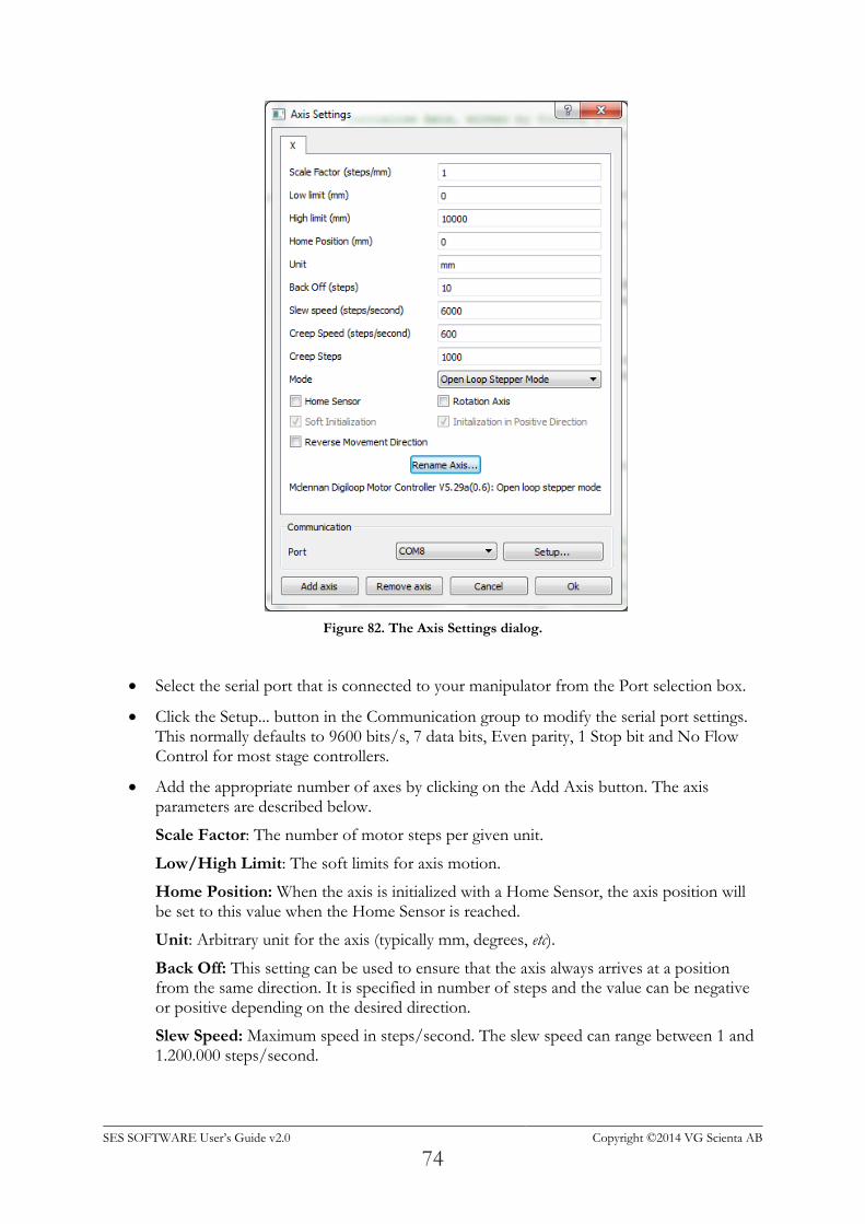
SES SOFTWARE User’s Guide v2.0 Copyright ©2014 VG Scienta AB
74
Figure 82. The Axis Settings dialog.
Select the serial port that is connected to your manipulator from the Port selection box.
Click the Setup... button in the Communication group to modify the serial port settings. This normally defaults to 9600 bits/s, 7 data bits, Even parity, 1 Stop bit and No Flow Control for most stage controllers.
Add the appropriate number of axes by clicking on the Add Axis button. The axis parameters are described below.
Scale Factor: The number of motor steps per given unit.
Low/High Limit: The soft limits for axis motion.
Home Position: When the axis is initialized with a Home Sensor, the axis position will be set to this value when the Home Sensor is reached.
Unit: Arbitrary unit for the axis (typically mm, degrees, etc).
Back Off: This setting can be used to ensure that the axis always arrives at a position from the same direction. It is specified in number of steps and the value can be negative or positive depending on the desired direction.
Slew Speed: Maximum speed in steps/second. The slew speed can range between 1 and 1.200.000 steps/second.
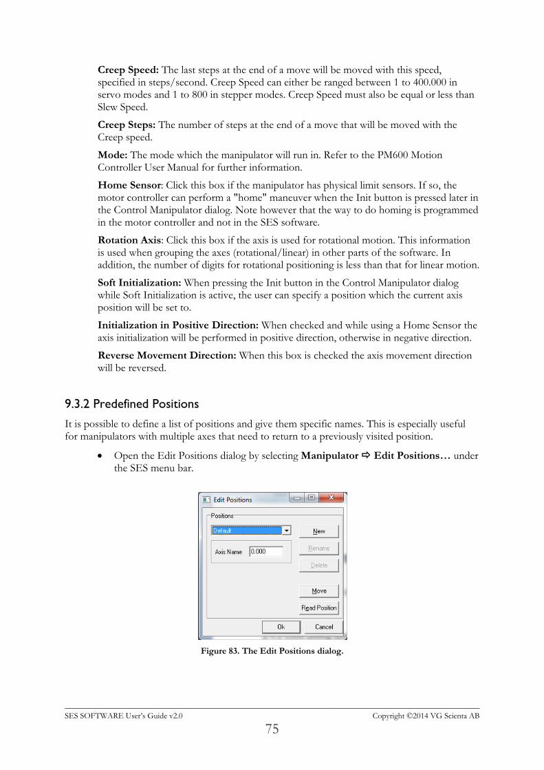
SES SOFTWARE User’s Guide v2.0 Copyright ©2014 VG Scienta AB
75
Creep Speed: The last steps at the end of a move will be moved with this speed, specified in steps/second. Creep Speed can either be ranged between 1 to 400.000 in servo modes and 1 to 800 in stepper modes. Creep Speed must also be equal or less than Slew Speed.
Creep Steps: The number of steps at the end of a move that will be moved with the Creep speed.
Mode: The mode which the manipulator will run in. Refer to the PM600 Motion Controller User Manual for further information.
Home Sensor: Click this box if the manipulator has physical limit sensors. If so, the motor controller can perform a "home" maneuver when the Init button is pressed later in the Control Manipulator dialog. Note however that the way to do homing is programmed in the motor controller and not in the SES software.
Rotation Axis: Click this box if the axis is used for rotational motion. This information is used when grouping the axes (rotational/linear) in other parts of the software. In addition, the number of digits for rotational positioning is less than that for linear motion.
Soft Initialization: When pressing the Init button in the Control Manipulator dialog while Soft Initialization is active, the user can specify a position which the current axis position will be set to.
Initialization in Positive Direction: When checked and while using a Home Sensor the axis initialization will be performed in positive direction, otherwise in negative direction.
Reverse Movement Direction: When this box is checked the axis movement direction will be reversed.
9.3.2 Predefined Positions
It is possible to define a list of positions and give them specific names. This is especially useful for manipulators with multiple axes that need to return to a previously visited position.
Open the Edit Positions dialog by selecting Manipulator Edit Positions… under the SES menu bar.
Figure 83. The Edit Positions dialog.
SES SOFTWARE User’s Guide v2.0 Copyright ©2014 VG Scienta AB
76
Click New to create a new position. The name of the position can be modified at any time by clicking on Rename.
Click Read Position to read the current position. This will update the values of all involved axes.
Modify the edit boxes in the available axes. To test the new position, click Move.
Close the dialog with Ok to accept the changes.
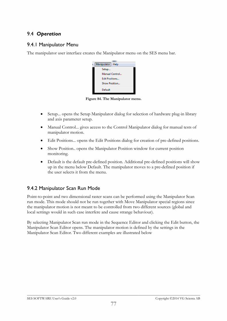
SES SOFTWARE User’s Guide v2.0 Copyright ©2014 VG Scienta AB
77
9.4 Operation
9.4.1 Manipulator Menu
The manipulator user interface creates the Manipulator menu on the SES menu bar.
Figure 84. The Manipulator menu.
Setup... opens the Setup Manipulator dialog for selection of hardware plug-in library and axis parameter setup.
Manual Control... gives access to the Control Manipulator dialog for manual tests of manipulator motion.
Edit Positions... opens the Edit Positions dialog for creation of pre-defined positions.
Show Position.. opens the Manipulator Position window for current position monitoring.
Default is the default pre-defined position. Additional pre-defined positions will show up in the menu below Default. The manipulator moves to a pre-defined position if the user selects it from the menu.
9.4.2 Manipulator Scan Run Mode
Point-to-point and two dimensional raster scans can be performed using the Manipulator Scan run mode. This mode should not be run together with Move Manipulator special regions since the manipulator motion is not meant to be controlled from two different sources (global and local settings would in such case interfere and cause strange behaviour). By selecting Manipulator Scan run mode in the Sequence Editor and clicking the Edit button, the Manipulator Scan Editor opens. The manipulator motion is defined by the settings in the Manipulator Scan Editor. Two different examples are illustrated below
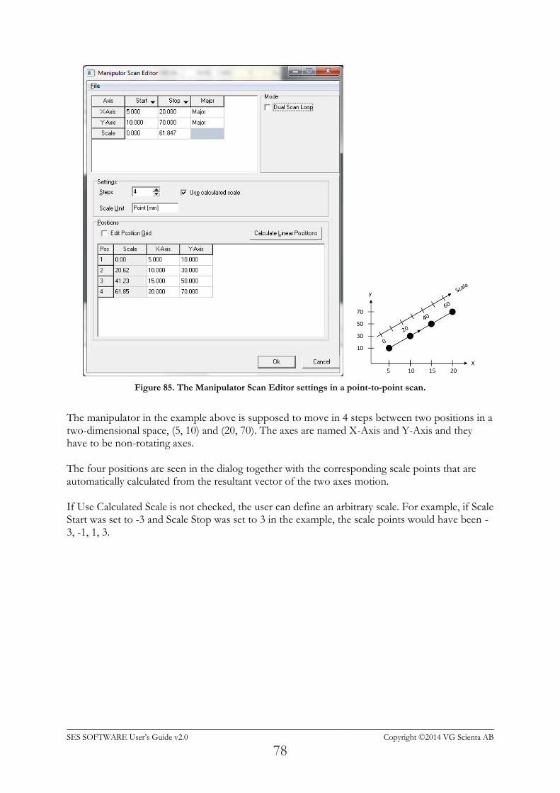
SES SOFTWARE User’s Guide v2.0 Copyright ©2014 VG Scienta AB
78
Figure 85. The Manipulator Scan Editor settings in a point-to-point scan.
The manipulator in the example above is supposed to move in 4 steps between two positions in a two-dimensional space, (5, 10) and (20, 70). The axes are named X-Axis and Y-Axis and they have to be non-rotating axes. The four positions are seen in the dialog together with the corresponding scale points that are automatically calculated from the resultant vector of the two axes motion. If Use Calculated Scale is not checked, the user can define an arbitrary scale. For example, if Scale Start was set to -3 and Scale Stop was set to 3 in the example, the scale points would have been -3, -1, 1, 3.
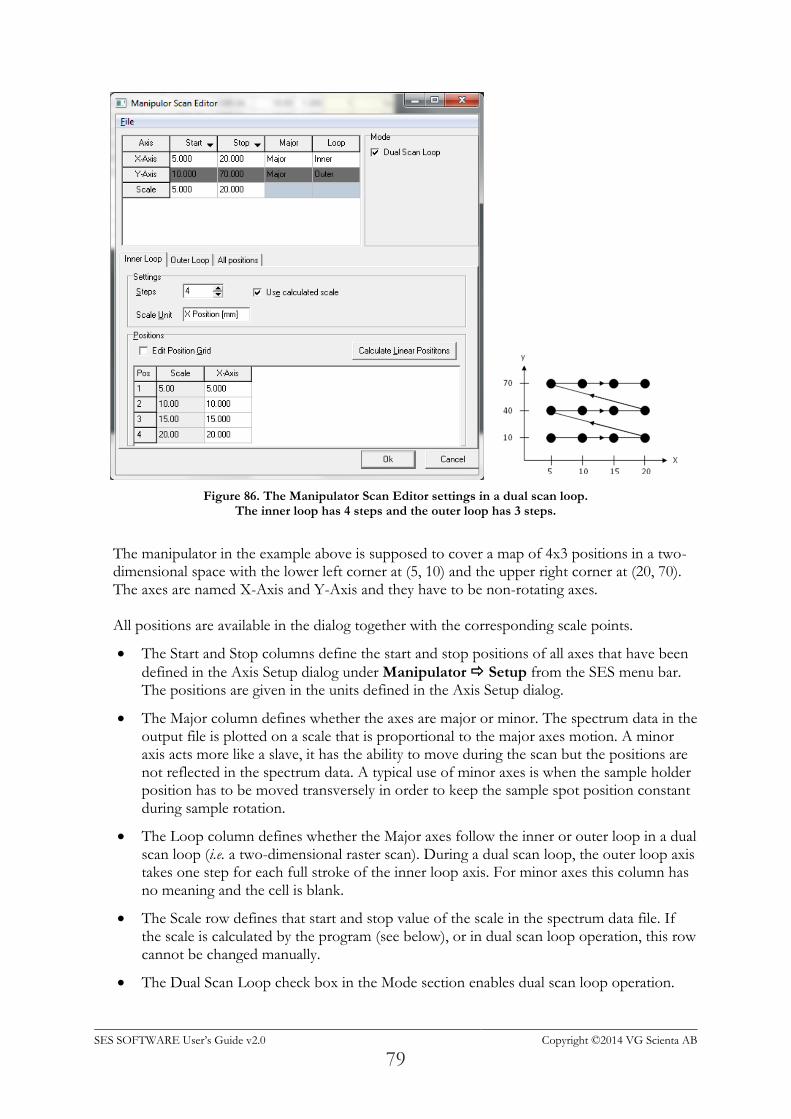
SES SOFTWARE User’s Guide v2.0 Copyright ©2014 VG Scienta AB
79
Figure 86. The Manipulator Scan Editor settings in a dual scan loop. The inner loop has 4 steps and the outer loop has 3 steps.
The manipulator in the example above is supposed to cover a map of 4x3 positions in a two-dimensional space with the lower left corner at (5, 10) and the upper right corner at (20, 70). The axes are named X-Axis and Y-Axis and they have to be non-rotating axes. All positions are available in the dialog together with the corresponding scale points.
The Start and Stop columns define the start and stop positions of all axes that have been
defined in the Axis Setup dialog under Manipulator Setup from the SES menu bar. The positions are given in the units defined in the Axis Setup dialog.
The Major column defines whether the axes are major or minor. The spectrum data in the output file is plotted on a scale that is proportional to the major axes motion. A minor axis acts more like a slave, it has the ability to move during the scan but the positions are not reflected in the spectrum data. A typical use of minor axes is when the sample holder position has to be moved transversely in order to keep the sample spot position constant during sample rotation.
The Loop column defines whether the Major axes follow the inner or outer loop in a dual scan loop (i.e. a two-dimensional raster scan). During a dual scan loop, the outer loop axis takes one step for each full stroke of the inner loop axis. For minor axes this column has no meaning and the cell is blank.
The Scale row defines that start and stop value of the scale in the spectrum data file. If the scale is calculated by the program (see below), or in dual scan loop operation, this row cannot be changed manually.
The Dual Scan Loop check box in the Mode section enables dual scan loop operation.
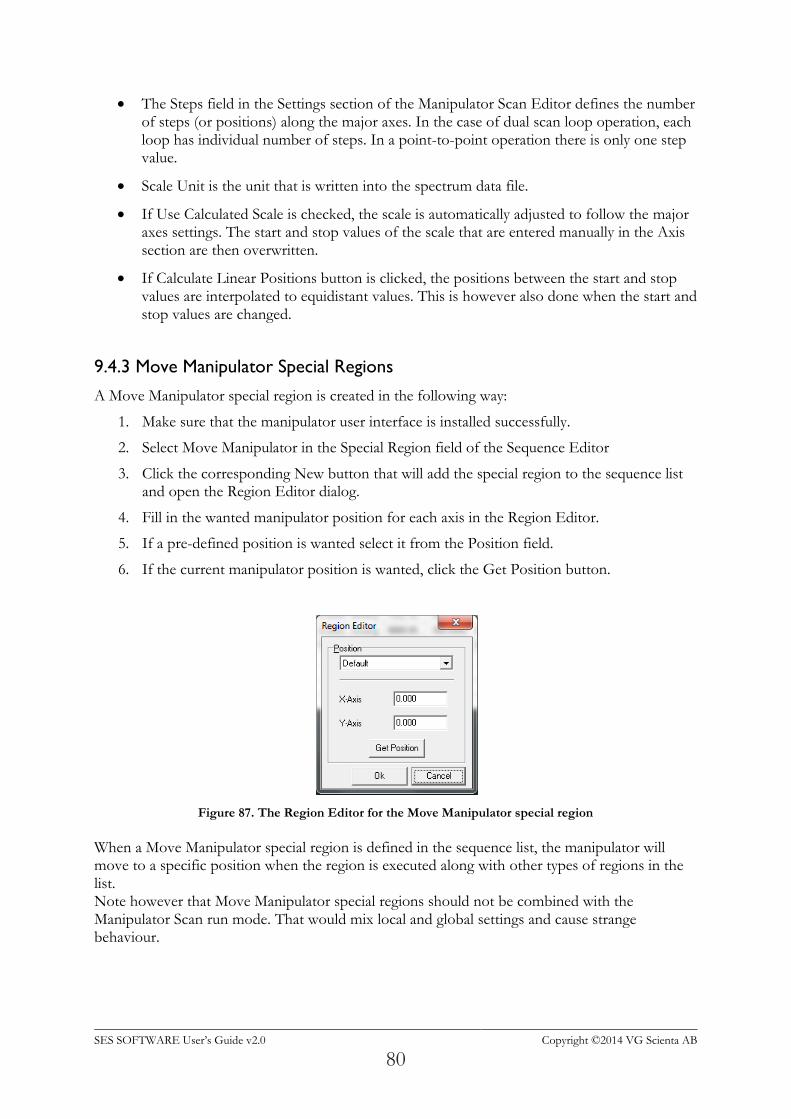
SES SOFTWARE User’s Guide v2.0 Copyright ©2014 VG Scienta AB
80
The Steps field in the Settings section of the Manipulator Scan Editor defines the number of steps (or positions) along the major axes. In the case of dual scan loop operation, each loop has individual number of steps. In a point-to-point operation there is only one step value.
Scale Unit is the unit that is written into the spectrum data file.
If Use Calculated Scale is checked, the scale is automatically adjusted to follow the major axes settings. The start and stop values of the scale that are entered manually in the Axis section are then overwritten.
If Calculate Linear Positions button is clicked, the positions between the start and stop values are interpolated to equidistant values. This is however also done when the start and stop values are changed.
9.4.3 Move Manipulator Special Regions
A Move Manipulator special region is created in the following way:
1. Make sure that the manipulator user interface is installed successfully.
2. Select Move Manipulator in the Special Region field of the Sequence Editor
3. Click the corresponding New button that will add the special region to the sequence list and open the Region Editor dialog.
4. Fill in the wanted manipulator position for each axis in the Region Editor.
5. If a pre-defined position is wanted select it from the Position field.
6. If the current manipulator position is wanted, click the Get Position button.
Figure 87. The Region Editor for the Move Manipulator special region
When a Move Manipulator special region is defined in the sequence list, the manipulator will move to a specific position when the region is executed along with other types of regions in the list. Note however that Move Manipulator special regions should not be combined with the Manipulator Scan run mode. That would mix local and global settings and cause strange behaviour.
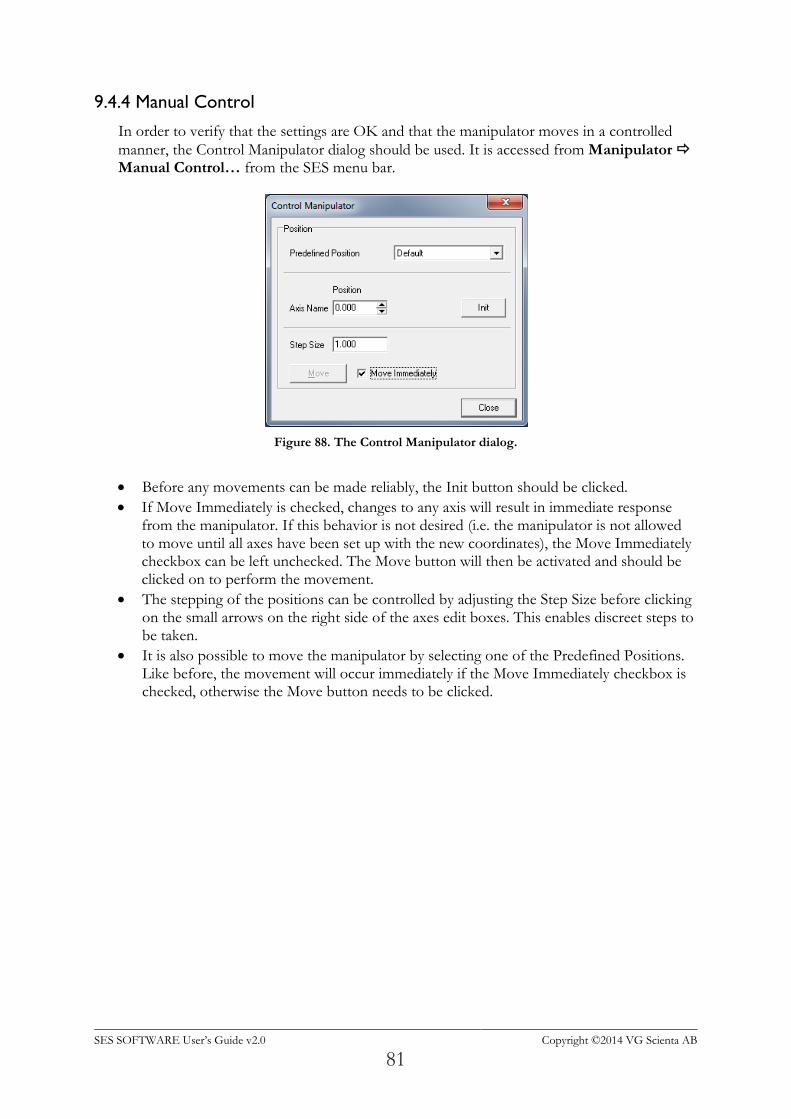
SES SOFTWARE User’s Guide v2.0 Copyright ©2014 VG Scienta AB
81
9.4.4 Manual Control
In order to verify that the settings are OK and that the manipulator moves in a controlled
manner, the Control Manipulator dialog should be used. It is accessed from Manipulator Manual Control… from the SES menu bar.
Figure 88. The Control Manipulator dialog.
Before any movements can be made reliably, the Init button should be clicked.
If Move Immediately is checked, changes to any axis will result in immediate response from the manipulator. If this behavior is not desired (i.e. the manipulator is not allowed to move until all axes have been set up with the new coordinates), the Move Immediately checkbox can be left unchecked. The Move button will then be activated and should be clicked on to perform the movement.
The stepping of the positions can be controlled by adjusting the Step Size before clicking on the small arrows on the right side of the axes edit boxes. This enables discreet steps to be taken.
It is also possible to move the manipulator by selecting one of the Predefined Positions. Like before, the movement will occur immediately if the Move Immediately checkbox is checked, otherwise the Move button needs to be clicked.
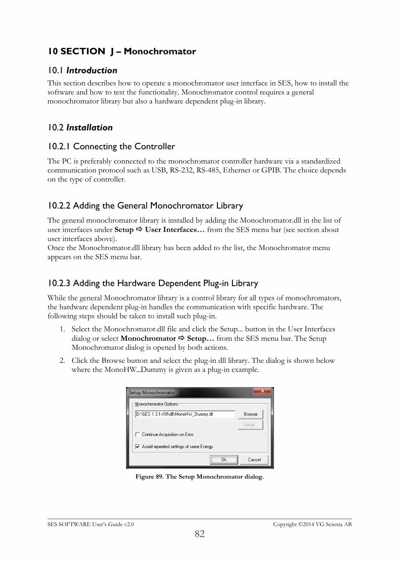
SES SOFTWARE User’s Guide v2.0 Copyright ©2014 VG Scienta AB
82
10 SECTION J – Monochromator
10.1 Introduction
This section describes how to operate a monochromator user interface in SES, how to install the software and how to test the functionality. Monochromator control requires a general monochromator library but also a hardware dependent plug-in library.
10.2 Installation
10.2.1 Connecting the Controller
The PC is preferably connected to the monochromator controller hardware via a standardized communication protocol such as USB, RS-232, RS-485, Ethernet or GPIB. The choice depends on the type of controller.
10.2.2 Adding the General Monochromator Library
The general monochromator library is installed by adding the Monochromator.dll in the list of
user interfaces under Setup User Interfaces… from the SES menu bar (see section about user interfaces above). Once the Monochromator.dll library has been added to the list, the Monochromator menu appears on the SES menu bar.
10.2.3 Adding the Hardware Dependent Plug-in Library
While the general Monochromator library is a control library for all types of monochromators, the hardware dependent plug-in handles the communication with specific hardware. The following steps should be taken to install such plug-in.
1. Select the Monochromator.dll file and click the Setup... button in the User Interfaces
dialog or select Monochromator Setup… from the SES menu bar. The Setup Monochromator dialog is opened by both actions.
2. Click the Browse button and select the plug-in dll library. The dialog is shown below where the MonoHW_Dummy is given as a plug-in example.
Figure 89. The Setup Monochromator dialog.
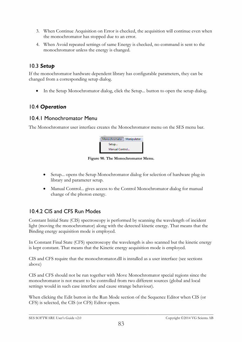
SES SOFTWARE User’s Guide v2.0 Copyright ©2014 VG Scienta AB
83
3. When Continue Acquisition on Error is checked, the acquisition will continue even when the monochromator has stopped due to an error.
4. When Avoid repeated settings of same Energy is checked, no command is sent to the monochromator unless the energy is changed.
10.3 Setup
If the monochromator hardware dependent library has configurable parameters, they can be changed from a corresponding setup dialog.
In the Setup Monochromator dialog, click the Setup... button to open the setup dialog.
10.4 Operation
10.4.1 Monochromator Menu
The Monochromator user interface creates the Monochromator menu on the SES menu bar.
Figure 90. The Monochromator Menu.
Setup... opens the Setup Monochromator dialog for selection of hardware plug-in library and parameter setup.
Manual Control... gives access to the Control Monochromator dialog for manual change of the photon energy.
10.4.2 CIS and CFS Run Modes
Constant Initial State (CIS) spectroscopy is performed by scanning the wavelength of incident light (moving the monochromator) along with the detected kinetic energy. That means that the Binding energy acquisition mode is employed. In Constant Final State (CFS) spectroscopy the wavelength is also scanned but the kinetic energy is kept constant. That means that the Kinetic energy acquisition mode is employed. CIS and CFS require that the monochromator.dll is installed as a user interface (see sections above) CIS and CFS should not be run together with Move Monochromator special regions since the monochromator is not meant to be controlled from two different sources (global and local settings would in such case interfere and cause strange behaviour). When clicking the Edit button in the Run Mode section of the Sequence Editor when CIS (or CFS) is selected, the CIS (or CFS) Editor opens.
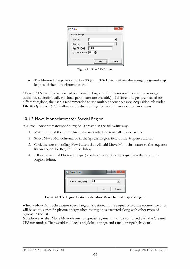
SES SOFTWARE User’s Guide v2.0 Copyright ©2014 VG Scienta AB
84
Figure 91. The CIS Editor.
The Photon Energy fields of the CIS (and CFS) Editor defines the energy range and step lengths of the monochromator scan.
CIS and CFS can also be selected for individual regions but the monochromator scan range cannot be set individually (no local parameters are available). If different ranges are needed for different regions, the user is recommended to use multiple sequences (see Acquisition tab under
File Options…). This allows individual settings for multiple monochromator scans.
10.4.3 Move Monochromator Special Region
A Move Monochromator special region is created in the following way:
1. Make sure that the monochromator user interface is installed successfully.
2. Select Move Monochromator in the Special Region field of the Sequence Editor
3. Click the corresponding New button that will add Move Monochromator to the sequence list and open the Region Editor dialog.
4. Fill in the wanted Photon Energy (or select a pre-defined energy from the list) in the Region Editor.
Figure 92. The Region Editor for the Move Monochromator special region
When a Move Monochromator special region is defined in the sequence list, the monochromator will be set to a specific photon energy when the region is executed along with other types of regions in the list. Note however that Move Monochromator special regions cannot be combined with the CIS and CFS run modes. That would mix local and global settings and cause strange behaviour.
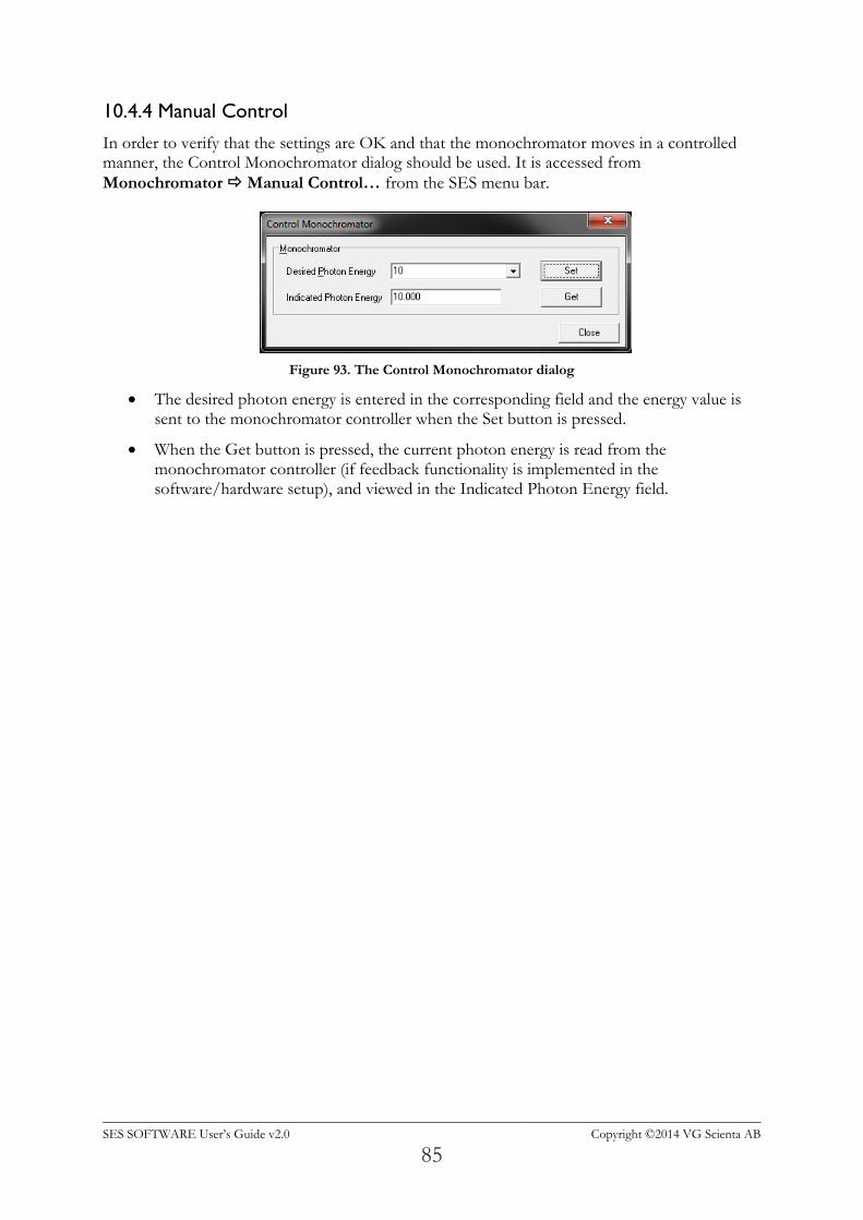
SES SOFTWARE User’s Guide v2.0 Copyright ©2014 VG Scienta AB
85
10.4.4 Manual Control
In order to verify that the settings are OK and that the monochromator moves in a controlled manner, the Control Monochromator dialog should be used. It is accessed from
Monochromator Manual Control… from the SES menu bar.
Figure 93. The Control Monochromator dialog
The desired photon energy is entered in the corresponding field and the energy value is sent to the monochromator controller when the Set button is pressed.
When the Get button is pressed, the current photon energy is read from the monochromator controller (if feedback functionality is implemented in the software/hardware setup), and viewed in the Indicated Photon Energy field.
SES SOFTWARE User’s Guide v2.0 Copyright ©2014 VG Scienta AB
86
11 SECTION K – DA30
The software features of the DA30 instrument are described in the DA30 Software User’s Guide document.
12 SECTION L – Single Transfer Spin
The software features of the Single Transfer Spin detector system are described in the Single Transfer Spin Software User’s Guide document.