uva-dare (digital academic repository) … benjamin kemper, joran lokkerbol and thijs vermaat....
TRANSCRIPT

UvA-DARE is a service provided by the library of the University of Amsterdam (http://dare.uva.nl)
UvA-DARE (Digital Academic Repository)
Estimation methods for statistical process controlSchoonhoven, M.
Link to publication
Citation for published version (APA):Schoonhoven, M. (2011). Estimation methods for statistical process control. Amsterdam: Universiteit vanAmsterdam.
General rightsIt is not permitted to download or to forward/distribute the text or part of it without the consent of the author(s) and/or copyright holder(s),other than for strictly personal, individual use, unless the work is under an open content license (like Creative Commons).
Disclaimer/Complaints regulationsIf you believe that digital publication of certain material infringes any of your rights or (privacy) interests, please let the Library know, statingyour reasons. In case of a legitimate complaint, the Library will make the material inaccessible and/or remove it from the website. Please Askthe Library: http://uba.uva.nl/en/contact, or a letter to: Library of the University of Amsterdam, Secretariat, Singel 425, 1012 WP Amsterdam,The Netherlands. You will be contacted as soon as possible.
Download date: 27 Mar 2019

Estimation Methods forStatistical Process Control

Dit proefschrift is mede mogelijk gemaakt door een financiele bijdrage vanhet Instituut voor Bedrijfs- en Industriele Statistiek van de Universiteit vanAmsterdam (IBIS UvA).
Omslagontwerp: Esther Ris (www.proefschriftomslag.nl)
ISBN: 978-90-6464-505-1

Estimation Methods forStatistical Process Control
ACADEMISCH PROEFSCHRIFT
ter verkrijging van de graad doctoraan de Universiteit van Amsterdamop gezag van de Rector Magnificus
prof.dr. D.C. van den Boomten overstaan van een door het college van promoties
ingestelde commissie,in het openbaar te verdedigen in de Agnietenkapelop woensdag 16 november 2011, te 14:00 uur
door
Marit Schoonhoven
geboren te Alphen aan den Rijn

Promotiecommissie
Promotor: Prof.dr. R.J.M.M. Does
Overige leden: Prof.dr. W. AlbersProf.dr. J.G. BethlehemProf.dr.ir. J.G. de GooijerProf.dr. C.A.J. KlaassenProf.dr. J. de MastProf.dr. K.C.B. RoesDr. A. Trip
Faculteit Economie en Bedrijfskunde

Preface
The thesis you have in front of you is the result of four years of hard work.But I could never have completed it without the help of many others. Inthis final phase, there are some people I would like to thank in particular.
The subject of the thesis is process control. I can’t think of anyonebetter able to control the research process than Ronald Does, my promoter.Ronald, I want to thank you for motivating me and accelerating the processat the right moments. I am sure that without you this process would nothave led to so many concrete results.
I would also like to thank Muhammad Riaz, whose creative ideas inspiredme and who collaborated with me on several articles.
The atmosphere at IBIS is very open and productive and working in suchan environment has been a great experience. I am indebted to all my currentand former IBIS colleagues for their generous advice on consultancy projects,research challenges and administrative issues whenever I found myself strug-gling. Thanks go to Atie Buisman, Henk de Koning, Jeroen de Mast, TashiErdmann, Benjamin Kemper, Joran Lokkerbol and Thijs Vermaat.
In realizing this book, I received help from two other people. I am gratefulto Ivette Jans for her textual improvements and Esther Ris for designing thecover.
Alongside hard work, it is good to relax. Here, I would like to thank myfriends and family, especially my parents Hans and Annemiek as well as Ilseand Niels, for always being there and always showing interest in my work.
Finally, I would like to thank Auke. Auke, you really helped me in allaspects of this thesis, not least with the technical Latex part, but mainlywith your love and all the pleasant moments we shared in the past four years.I look forward to the future together filled with many more challenges.
Marit SchoonhovenNovember 2011
v


Contents
Preface v
1 Introduction 1
1.1 Shewhart control charts . . . . . . . . . . . . . . . . . . . . . 1
1.2 Contributions and thesis outline . . . . . . . . . . . . . . . . 5
2 Standard Deviation Control Charts 11
2.1 Introduction . . . . . . . . . . . . . . . . . . . . . . . . . . . . 11
2.2 Proposed Phase I estimators . . . . . . . . . . . . . . . . . . . 11
2.2.1 Standard deviation estimators . . . . . . . . . . . . . . 12
2.2.2 Efficiency of proposed estimators . . . . . . . . . . . . 17
2.3 Derivation of Phase II control limits . . . . . . . . . . . . . . 25
2.4 Control chart performance . . . . . . . . . . . . . . . . . . . . 26
2.4.1 Simulation procedure . . . . . . . . . . . . . . . . . . 27
2.4.2 Simulation results . . . . . . . . . . . . . . . . . . . . 27
2.5 Real data example . . . . . . . . . . . . . . . . . . . . . . . . 42
2.6 Concluding remarks . . . . . . . . . . . . . . . . . . . . . . . 45
2.7 Appendix . . . . . . . . . . . . . . . . . . . . . . . . . . . . . 45
3 A Robust Standard Deviation Control Chart 47
3.1 Introduction . . . . . . . . . . . . . . . . . . . . . . . . . . . . 47
3.2 Proposed Phase I estimators . . . . . . . . . . . . . . . . . . . 48
3.2.1 Standard deviation estimators . . . . . . . . . . . . . . 48
3.2.2 Real data example . . . . . . . . . . . . . . . . . . . . 50
3.2.3 Efficiency of proposed estimators . . . . . . . . . . . . 53
3.3 Derivation of Phase II control limits . . . . . . . . . . . . . . 59
3.4 Control chart performance . . . . . . . . . . . . . . . . . . . . 59
3.4.1 Simulation procedure . . . . . . . . . . . . . . . . . . 60
vii

viii Contents
3.4.2 Simulation results . . . . . . . . . . . . . . . . . . . . 603.5 Concluding remarks . . . . . . . . . . . . . . . . . . . . . . . 64
4 Location Estimators for X Control Charts 654.1 Introduction . . . . . . . . . . . . . . . . . . . . . . . . . . . . 654.2 Proposed location estimators . . . . . . . . . . . . . . . . . . 66
4.2.1 Location estimators . . . . . . . . . . . . . . . . . . . 664.2.2 Efficiency of proposed estimators . . . . . . . . . . . . 69
4.3 Proposed control chart location estimators . . . . . . . . . . . 734.3.1 Phase I control charts . . . . . . . . . . . . . . . . . . 734.3.2 Efficiency of proposed Phase I control charts . . . . . 77
4.4 Derivation of Phase II control limits . . . . . . . . . . . . . . 804.5 Control chart performance . . . . . . . . . . . . . . . . . . . . 81
4.5.1 Simulation procedure . . . . . . . . . . . . . . . . . . 814.5.2 Simulation results . . . . . . . . . . . . . . . . . . . . 82
4.6 Concluding remarks . . . . . . . . . . . . . . . . . . . . . . . 89
5 A Robust X Control Chart 915.1 Introduction . . . . . . . . . . . . . . . . . . . . . . . . . . . . 915.2 Proposed Phase I estimators . . . . . . . . . . . . . . . . . . . 92
5.2.1 Standard deviation estimators . . . . . . . . . . . . . . 925.2.2 Location estimator . . . . . . . . . . . . . . . . . . . . 945.2.3 Efficiency of proposed standard deviation estimators . 95
5.3 Derivation of Phase II control limits . . . . . . . . . . . . . . 1015.4 Control chart performance . . . . . . . . . . . . . . . . . . . . 102
5.4.1 Simulation procedure . . . . . . . . . . . . . . . . . . 1025.4.2 Simulation results . . . . . . . . . . . . . . . . . . . . 103
5.5 Concluding remarks . . . . . . . . . . . . . . . . . . . . . . . 105
Bibliography 117
Samenvatting 121
Curriculum Vitae 125
Chapter 1
Introduction
This chapter gives a short introduction to Shewhart control charts, an over-view of new developments and an outline of the thesis.
1.1 Shewhart control charts
Processes are subject to variation. Whether or not a given process is func-tioning normally can be evaluated with control charts. Such charts showwhether the variation is entirely due to common causes or whether some ofthe variation is due to special causes. Variation due to common causes isinevitable: it is generated by the design and standard operations of the pro-cess. When the process variation is due to common causes only, the processis said to be in statistical control. In this case, the process fluctuates withina predictable bandwidth. Special causes of process variation may consist ofsuch factors as extraordinary events, unexpected incidents, or a new sup-plier for incoming material. For optimal process performance, such specialcauses should be detected as soon as possible and prevented from occurringagain. Control charts are used to signal the occurrence of a special cause.The power of the control chart lies partly in its simplicity: it consists of agraph of a process characteristic plotted through time. The control limitsin the graph provide easy checks on the stability of the process (i.e. nospecial causes present). The concept of control charts originates with She-whart (1931) and has been extensively discussed and extended in numeroustextbooks (see e.g. Duncan (1986), Does et al. (1999) and Montgomery(2009)).
In the standard situation, 20-30 samples of about five units are taken
1

2 Introduction
initially to construct a control chart. When a process characteristic is anumerical variable, it is standard practice to control both the mean value ofthe characteristic and its spread. The control limits of the statistic of interestare calculated as the average of the sample mean or standard deviation plusor minus a multiplier times the standard deviation of the statistic. Thespread parameter of the process is controlled first, followed by the locationparameter. An example of such a combined standard deviation and locationchart is given in Figure 1.1.
The general set-up of a Shewhart control chart for the dispersion param-eter is as follows. Let Yij , i = 1, 2, 3, ... and j = 1, 2, ..., n, denote samplesof size n taken in sequence of the process variable to be monitored. Weassume the Yij ’s to be independent and N(μ, (λσ)2) distributed, where λ isa constant. When λ = 1, the standard deviation of the process is in control;otherwise the standard deviation has changed. Let σi be an estimate of λσbased on the i-th sample Yij , j = 1, 2, ..., n. Usually, λσ is estimated by thesample standard deviation S. When the in-control σ is known, the processstandard deviation can be monitored by plotting σi on a standard deviationcontrol chart with respective upper and lower control limits
UCL = Unσ, LCL = Lnσ, (1.1)
where Un and Ln are factors such that for a chosen type I error probabilityα we have
P (Lnσ ≤ σi ≤ Unσ) = 1− α.
When σi falls within the control limits, the spread is deemed to be in control.For the location control chart, the Yij ’s, i = 1, 2, 3, ... and j = 1, 2, .., n,
again denote samples of the process variable to be monitored. In this case,we assume the Yij ’s to be independent and N(μ+ δσ, σ2) distributed, whereδ is a constant. When δ = 0, the mean of the process is in control; otherwisethe process mean has changed. Let Yi =
1n
∑nj=1 Yij be an estimate of μ+δσ
based on the i-th sample Yij , j = 1, 2, ..., n. When the in-control μ and σare known, the process mean can be monitored by plotting Yi on a locationcontrol chart with respective upper and lower control limits
UCL = μ+ Cnσ/√n, LCL = μ− Cnσ/
√n, (1.2)
where Cn is the factor such that for a chosen type I error probability α wehave
P (LCL ≤ Yi ≤ UCL) = 1− α.

1.1 Shewhart control charts 3
2 4 6 8 10 12 14 16 18 200
2
4
6
8
10
12
14
16
18
20
Sample number
S
Upper control limit
Lower control limit
2 4 6 8 10 12 14 16 18 2028
30
32
34
36
38
40
Sample number
X
Upper control limit
Lower control limit
Figure 1.1: Standard deviation and location control chart

4 Introduction
When Yi falls within the control limits, the location of the process is deemedto be in control.
The performance of the spread control chart is evaluated in the sameway as that of the location control chart. We define Ei as the event thatσi (Yi) falls beyond the control limits, P (Ei) as the probability that σi (Yi)falls beyond the limits and RL as the run length, i.e. the number of samplesdrawn until the first σi (Yi) falls beyond the limits. When σ (μ, σ) is known,the events Ei are independent, and therefore RL is geometrically distributedwith parameter p = P (Ei) = α. It follows that the average run length (ARL)is given by 1/p and that the standard deviation of the run length (SDRL) isgiven by
√1− p/p.
In practice, the in-control process parameters are usually unknown. There-fore, they must be estimated from k samples of size n taken when the pro-cess is assumed to be in control. This stage in the control charting processis called Phase I (cf. Woodall and Montgomery (1999) and Vining (2009)).The monitoring stage is denoted by Phase II. The samples used to estimatethe process parameters are denoted by Xij , i = 1, 2, ..., k and j = 1, 2, ..., n.Define σ and μ as the unbiased estimates of σ and μ respectively, based onthe Xij . The control limits are estimated by
UCL = Unσ, LCL = Lnσ (1.3)
for the standard deviation control chart and
UCL = μ+ Cnσ/√n, LCL = μ− Cnσ/
√n (1.4)
for the location control chart.Note that Un, Ln and Cn in (1.3) and (1.4) are not necessarily the same
as in (1.1) and (1.2) and might be different even when the probability ofsignaling is the same. Below, we describe how we evaluate the standarddeviation control chart with estimated parameters. The location chart withestimated parameters is evaluated in the same way. Let Fi denote the eventthat σi is above UCL or below LCL. We define P (Fi|σ) as the probabilitythat sample i generates a signal given σ, i.e.
P (Fi|σ) = P (σi < LCL or σi > UCL|σ). (1.5)
Given σ, the distribution of the run length is geometric with parameterP (Fi|σ). Consequently, the conditional ARL is given by
E(RL|σ) = 1
P (Fi|σ) . (1.6)

1.2 Contributions and thesis outline 5
In contrast with the conditional RL distribution, the unconditional RLdistribution takes into account the random variability introduced into thecharting procedure through parameter estimation. It can be obtained byaveraging the conditional RL distribution over all possible values of the pa-rameter estimates. The unconditional p is
p = E(P (Fi|σ)), (1.7)
the unconditional average run length is
ARL = E(1
P (Fi|σ)) (1.8)
and the unconditional standard deviation of the run length is determined by
SDRL =√
V ar(RL)
=√
E(V ar(RL|σ)) + V ar(E(RL|σ))=
√2E( 1
p(Fi|σ))2 − (E 1
p(Fi|σ))2 − E 1
p(Fi|σ) .(1.9)
Quesenberry (1993) showed that for the X and X control charts theunconditional ARL is higher than in the (μ,σ)-known case. Furthermore, ahigher in-control ARL is not necessarily better because the RL distributionwill reflect an increased number of short RL’s as well as an increased numberof long RL’s. He concluded that, if limits are to behave like known limits, thenumber of samples (k) in Phase I should be at least 400/(n-1) for X controlcharts and 300 for X control charts. Chen (1998) studied the unconditionalRL distribution of the standard deviation control chart under normality. Heshowed that if the shift in the standard deviation in Phase II is large, theimpact of parameter estimation is small. In order to achieve a performancecomparable with known limits, he recommended taking at least 30 samplesof size 5 and updating the limits when more samples become available. Forpermanent limits, at least 75 samples of size 5 should be used. Thus, thesituation is somewhat better than for the X control chart with both processmean and standard deviation estimated.
1.2 Contributions and thesis outline
Jensen et al. (2006) conducted a literature survey of the effects of parame-ter estimation on control chart properties and identified the following issue
6 Introduction
for future research: “The effect of using robust or other alternative estima-tors has not been studied thoroughly. Most evaluations of performance haveconsidered standard estimators based on the sample mean and the standarddeviation and have used the same estimators for both Phase I and Phase II.However, in Phase I applications it seems more appropriate to use an esti-mator that will be robust to outliers, step changes and other data anomalies.Examples of robust estimation methods in Phase I control charts includeRocke (1989), Rocke (1992), Tatum (1997), Vargas (2003) and Davis andAdams (2005). The effect of using these robust estimators on Phase II per-formance is not clear, but it is likely to be inferior to the use of standardestimates because robust estimators are generally not as efficient” (Jensen etal. 2006, p. 360). This recommendation is the main subject of the thesis. Inparticular, we will study alternative estimators in Phase I and we will studythe impact of these estimators on the performance of the Phase II controlchart.
Chen (1998) studied the standard deviation control chart when σ is es-timated by the pooled sample standard deviation (S), the mean samplestandard deviation (S) or the mean sample range (R) under normality. Heshowed that the performance of the charts based on S and S is almost iden-tical, while the performance of the chart based on R is slightly worse. Rocke(1989) proposed robust control charts based on the 25% trimmed mean of thesample ranges, the median of the sample ranges and the mean of the sampleinterquartile ranges in contaminated Phase I situations. Moreover, he stud-ied the use of a two-stage procedure whereby the initial chart is constructedfirst and then subgroups that seem to be out of control are excluded. Rocke(1992) gave the practical details for the construction of these charts. Wuet al. (2002) considered three alternative statistics for the sample standarddeviation, namely the median of the absolute deviation from the median(MDM), the average absolute deviation from the median (ADM) and themedian of the average absolute deviation (MAD), and investigated their ef-fect on X control chart performance. They concluded that, if there are no oronly a few contaminations in the Phase I data, ADM performs best. Other-wise, MDM is the best estimator. Riaz and Saghir (2007 and 2009) showedthat the statistics for the sample standard deviation based on Gini’s meandifference and the ADM are robust against non-normality. However, theyonly considered the situation where a large number of samples is availablein Phase I and did not consider contaminations in Phase I. Tatum (1997)clearly distinguished two types of disturbances: diffuse and localized. Dif-

1.2 Contributions and thesis outline 7
fuse disturbances are outliers that are spread over multiple samples whereaslocalized disturbances affect all observations in a single sample. He proposeda method, constructed around a variant of the biweight A estimator, that isresistant to both diffuse and localized disturbances. A result of the inclusionof the biweight A estimator is, however, that the method is relatively com-plicated in its use. Apart from several range-based methods, Tatum did notcompare his method with other methods for Phase I estimation. Finally,Boyles (1997) studied the dynamic linear model estimator for individualscharts (see also Braun and Park (2008)).
In Chapter 2 we compare an extensive number of Phase I estimatorsthat have been presented in the literature and a number of variants of thesestatistics. We study their effect on the Phase II performance of the stan-dard deviation control chart. The estimators considered are S, S, the 25%trimmed mean of the sample standard deviations, the mean of the samplestandard deviations after trimming the observations in each sample, R, thesample interquartile range, Gini’s mean difference, the MDM , the ADM ,theMAD, and the robust estimator of Tatum (1997). Moreover, we proposea robust estimation method based on the mean absolute deviation from themedian supplemented with a simple screening method. The performanceof the estimators is evaluated by assessing the mean squared error (MSE)of the estimators under normality and in the presence of various types ofcontaminations. Finally, we assess the Phase II performance of the controlcharts by means of a simulation study.
Most of the standard deviation estimators presented in Chapter 2 arerobust against either diffuse disturbances, i.e. outliers spread over the sam-ples, or localized disturbances, which affect an entire sample. In Chapter3 we therefore propose an algorithm that is robust against both types ofdisturbances. The method is compared with the pooled standard deviation(because this estimator is most efficient under normality), the robust esti-mator of Tatum (1997) and several adaptive trimmers. The performance ofthe estimators is evaluated by assessing the MSE of the estimators in sev-eral situations. Furthermore, we derive factors for the Phase II limits of thestandard deviation control chart and assess the performance of the Phase IIcontrol charts by means of a simulation study.
As noted earlier, the dispersion parameter of the process is controlledfirst, followed by the location parameter.
So far the literature has proposed several alternative robust location esti-mators. Rocke (1989) proposed the 25% trimmed mean of the sample means,
8 Introduction
the median of the sample means and the mean of the sample medians. Rocke(1992) followed with the practical details for the construction of the corre-sponding charts. Alloway and Raghavachari (1991) constructed a controlchart based on the Hodges-Lehmann estimator. Tukey (1997) and Wang etal. (2007) developed the trimean estimator, which is defined as the weightedaverage of the median and the two other quartiles. Finally, Jones-Farmer etal. (2009) proposed a rank-based Phase I location control chart. Based onthis control chart, they define the in-control state of a process and identifyan in-control reference dataset to estimate the location parameter.
In Chapter 4 we consider several robust location estimators as well asseveral estimation methods based on a Phase I analysis, whereby a controlchart is used to study a historical dataset retrospectively and thus identifydisturbances. In addition, we propose a new type of Phase I analysis. Themethods are evaluated in terms of their MSE and their effect on X Phase IIcontrol chart performance. We consider situations where the Phase I dataare uncontaminated and normally distributed, as well as various types ofcontaminated Phase I situations.
The results of Chapter 4 indicate that the X Phase II control chart (withσ known) based on the new estimation method performs well under normal-ity and outperforms the other charts when contaminations are present inPhase I. However, the results indicate that the effect of estimating the pro-cess location on the performance of the X Phase II control chart is more lim-ited than the effect of the standard deviation estimator. Chapter 5 thereforelooks at the effect of alternative standard deviation estimators under variousPhase I scenarios.
In Chapter 5 we develop an estimation method to derive the standarddeviation for the X control chart when both μ and σ are unknown. Apartfrom the new method, several alternative estimation methods are included inthe comparison. The methods are evaluated in terms of their MSE and theireffect on X Phase II control chart performance. We again consider the situ-ation where the Phase I data are uncontaminated and normally distributed,as well as various types of contaminated Phase I situations.
The material presented in Chapters 2-5 has led to four papers in variousstages of publication. The analysis in Chapter 2 has been published in theJournal of Quality Technology (Schoonhoven et al. (2011b)). A follow-up pa-per based on Chapter 3 has been accepted for publication in Technometrics,with minor revisions (Schoonhoven and Does (2011a)). The work in Chap-ter 4 has been published in the Journal of Quality Technology (Schoonhoven

1.2 Contributions and thesis outline 9
et al. (2011a)) and a follow-up article based on the material in Chapter 5has been submitted to the Journal of Quality Technology (Schoonhoven andDoes (2011b)).

Chapter 2
Standard Deviation Control Charts
2.1 Introduction
This chapter concerns the design and analysis of the standard deviation con-trol chart with estimated limits. We consider an extensive range of statisticsto estimate the in-control standard deviation (Phase I) and design the controlchart for real-time process monitoring (Phase II) by determining the factorsfor the control limits. The Phase II performance of the design schemes is as-sessed when the Phase I data are uncontaminated and normally distributedas well as when the Phase I data are contaminated. We propose a robustestimation method based on the mean absolute deviation from the mediansupplemented with a simple screening method.
The chapter is structured as follows. The next section introduces variousestimators of the standard deviation and assesses the MSE of the estimators.We then derive the Phase II control limits. Next, we describe the simula-tion procedure and simulation results. Furthermore, we discuss a real-worldexample implementing the various charts created. The chapter ends withsome concluding remarks.
2.2 Proposed Phase I estimators
In practice the same statistic is generally used to estimate both the in-controlstandard deviation σ in Phase I and the standard deviation λσ in Phase II.Since the requirements for the estimators differ between the two phases, thisis not always the best choice. In Phase I, an estimator should be efficientin uncontaminated situations and robust against disturbances, whereas in
11
12 Standard Deviation Control Charts
Phase II the estimator should be sensitive to disturbances (cf. Jensen et al.(2006)). In the next two sections, we present the Phase I estimators consid-ered in our study (Section 2.2.1) and evaluate the estimators by comparingtheir MSE (Section 2.2.2).
2.2.1 Standard deviation estimators
David (1998) gave a brief account of the history of standard deviation esti-mators. The traditional estimators are of course the pooled and the meansample standard deviation and the mean sample range. Mahmoud et al.(2010) studied the relative efficiencies of these estimators for different sam-ple sizes n and numbers of samples k. In deriving estimates of the in-controlstandard deviation, we will look at these as well as nine other estimators.
The first estimator of σ is based on the pooled sample standard deviation
S =
(1
k
k∑i=1
S2i
)1/2
, (2.1)
where Si is the i-th sample standard deviation defined by
Si =
(1
n− 1
n∑j=1
(Xij − Xi)2
)1/2
.
An unbiased estimator is given by S/c4(k(n−1)+1), where c4(m) is definedby
c4(m) =
(2
m− 1
)1/2 Γ(m/2)
Γ((m− 1)/2).
The second estimator is based on the mean sample standard deviation
S =1
k
k∑i=1
Si. (2.2)
An unbiased estimator of σ is given by S/c4(n).
Rocke (1989) proposed the trimmed mean of the sample ranges. In ourstudy, we consider a variant of this estimator, namely the trimmed meanof the sample standard deviations because it is well known that the sample

2.2 Proposed Phase I estimators 13
standard deviation is more robust than the sample range. The trimmedmean of the sample standard deviations is given by
Sa =1
k − �ka�×[ k−�ka�∑
v=1
S(v)
], (2.3)
where a denotes the percentage of samples to be trimmed, �z� denotes thesmallest integer not less than z and S(v) denotes the v-th ordered valueof the sample standard deviations. We consider the 25% trimmed meanof the sample standard deviations. To simplify the analysis, we trim aninteger number of samples. For example, the 25% trimmed mean trims offthe eight largest sample standard deviations when k = 30. To provide anunbiased estimate of σ for the normal case, the estimate must be divided by anormalizing constant. These constants are obtained from 100,000 simulationruns. For n = 5 and k = 20, 30, 75, the constants are 0.579, 0.585 and 0.568respectively; for n = 9 and k = 20, 30, 75, the constants are 0.701, 0.705 and0.693 respectively.
Because the above estimator trims off samples instead of individual obser-vations, we expect the estimator to be robust against localized disturbances.We also consider a variant that is expected to be robust against diffuse dis-turbances, namely the mean sample standard deviation after trimming theobservations in each sample
Sb =1
k
k∑i=1
S′i, (2.4)
where S′i is the standard deviation of sample i after trimming the observa-tions, given by
S′i =(
1
n− 2�nb� − 1
n−�nb�∑v=�nb�+1
(Xi(v) − X ′i)2
)1/2
,
where
X ′i =
1
n− 2�nb�n−�nb�∑
v=�nb�+1
Xi(v),
with Xi(v) the v-th ordered value in sample i and b the percentage of lowestand highest observations to be trimmed in each sample. In this study, we
14 Standard Deviation Control Charts
take 20% as our trimming percentage and, again, we trim an integer numberof observations. The estimator trims off the smallest and largest observationfor n = 5; it trims off the two smallest and the two largest observations forn = 9. The normalizing constant is 0.520 for n = 5 and 0.473 for n = 9.
The next estimator is based on the mean sample range
R =1
k
k∑i=1
Ri, (2.5)
where Ri is the range of the i-th sample. An unbiased estimator of σ isR/d2(n), where d2(n) is the expected range of a random N(0, 1) sample ofsize n. Values of d2(n) can be found in Duncan (1986), Table M.
The next estimator is based on the mean of the sample interquartileranges
IQR =1
k
k∑i=1
IQRi, (2.6)
with IQRi the interquartile range of sample i
IQRi = Xi(n−�ne�) −Xi(�ne�+1).
Thus, the same observations are trimmed off as in the calculation of S′i.(Note that one would expect the IQR to correspond to e = 0.25. However,to simplify the analysis we only trim an integer number of observations.)The normalizing constant is 0.990 for n = 5 and 1.144 for n = 9.
We also consider an estimator based on the mean of the sample Gini’smean differences
G =1
k
k∑i=1
Gi, (2.7)
where Gi is Gini’s mean difference of sample i, defined by
Gi =
n−1∑j=1
n∑l=j+1
|Xij −Xil|/(n(n− 1)/2),
representing the mean absolute difference between any two observations inthe sample. This statistic was proposed by Gini (1912), although basicallythe same statistic had already been proposed by Jordan (1869). An unbiasedestimator of σ is given by G/d2(2). The appendix shows that the estimator

2.2 Proposed Phase I estimators 15
based on Gini’s mean difference can be rewritten as a linear function of orderstatistics and that Gini’s mean difference is essentially the same as the so-called Downton estimator (Downton (1966)) and the probability-weightedmoments estimator (Muhammad et al. (1993)). From David (1981, p. 191)it follows that the estimator derived from Gini’s mean difference is highlyefficient (98%) and is more robust to outliers than the estimators based onR or S.
An estimator of σ that is simpler and easier to interpret uses the meanof the sample average absolute deviation from the median, given by
ADM =1
k
k∑i=1
ADMi, (2.8)
where ADMi is the average absolute deviation from the median of samplei, defined as
ADMi =1
n
n∑j=1
|Xij −Mi|,
with Mi the median of sample i. An unbiased estimator of σ is given byADM/t2(n). Since it is difficult to obtain the constant t2(n) analytically,it is obtained by simulation. Extensive tables of t2(n) can be found in Riazand Saghir (2009).
We also study the above estimator supplemented with a screening methodbased on control charting. Rocke (1989) proposed a two-stage procedurewhich first estimates σ by R, then deletes any sample that exceeds the con-trol limits and recomputes R using the remaining samples. Our approachfollows a similar procedure. First, we estimate σ by ADM because ADMis expected to be more robust against outliers. For simplicity, our screeningmethod uses the well known factors of the S/c4(n) control chart correspond-ing to the 3σ control limits in Phase I. Hence, the factors for the limits are2.089 and 0 for n = 5 and 1.761 and 0.239 for n = 9 (cf. Table M in Duncan(1986)). We then chart S/c4(n), delete any sample that exceeds the controllimits and recompute ADM using the remaining samples. We continue untilall sample estimates fall within the limits. The normalizing constant is 0.996for n = 5 and 0.998 for n = 9. The resulting estimator is denoted by ADM ′.
Next we study two other median statistics, namely the average of the
16 Standard Deviation Control Charts
sample medians of the absolute deviation from the median
MDM =1
k
k∑i=1
MDMi, (2.9)
withMDMi = median{|Xij −Mi|},
and the mean of the sample medians of the average absolute deviation
MAD =1
k
k∑i=1
MADi, (2.10)
withMADi = median{|Xij −Xi|}.
The normalizing constant for MDM is 0.554 for n = 5 and 0.613 for n = 9.For MAD, the normalizing constant is 0.627 for n = 5 and 0.658 for n = 9.
We also evaluate a robust estimator proposed by Tatum (1997). Hismethod has proven to be robust to both diffuse and localized disturbances.The estimation method is constructed around a variant of the biweight Aestimator. The method begins by calculating the residuals in each sample,which involves substracting the sample median from each value: resij =Xij −Mi. If n is odd, then in each sample one of the residuals will be zeroand is dropped. As a result, the total number of residuals is equal tom′ = nkwhen n is even and m′ = (n−1)k when n is odd. Tatum’s estimator is givenby
S∗c =m′
(m′ − 1)1/2
(∑k
i=1
∑j:|uij |<1 res
2ij(1− u2ij)
4)1/2
|∑ki=1
∑j:|uij |<1(1− u2ij)(1− 5u2ij)|
, (2.11)
where uij = hiresij/(cM∗), M∗ is the median of the absolute values of all
residuals,
hi =
⎧⎨⎩
1 Ei ≤ 4.5,Ei − 3.5 4.5 < Ei ≤ 7.5,c Ei > 7.5,
and Ei = IQRi/M∗. The constant c is a tuning constant. Each value
of c leads to a different estimator. Tatum showed that c = 7 gives anestimator that loses some efficiency when no disturbances are present, butgains efficiency when disturbances are present. We apply this value of c in

2.2 Proposed Phase I estimators 17
our simulation study. Note that we have h(i) = Ei − 3.5 for 4.5 < Ei ≤ 7.5in the equations instead of h(i) = Ei − 4.5 as presented by Tatum (Tatum1997, p. 129). This was a typographical error in the formula, resulting intoo much weight on localized disturbances and thus an overestimation of σ.An unbiased estimator of σ is given by S∗c /d∗(c, n, k), where d∗(c, n, k) isthe normalizing constant. During the implementation of the estimator wediscovered that, for odd values of n, the values of d∗(c, n, k) given by Table1 in Tatum (1997) should be corrected. We use the corrected values, whichare presented in Table 2.1 below. The resulting estimator is denoted by D7as in Tatum (1997).
c = 7 c = 10n k = 20 k = 30 k = 40 k = 75 k = 20 k = 30 k = 40 k = 755 1.070 1.069 1.068 1.068 1.054 1.053 1.053 1.0527 1.057 1.056 1.056 1.056 1.041 1.040 1.040 1.0409 1.052 1.051 1.050 1.050 1.034 1.034 1.033 1.03311 1.047 1.046 1.046 1.046 1.029 1.029 1.028 1.02813 1.044 1.044 1.043 1.043 1.026 1.025 1.025 1.02515 1.041 1.041 1.041 1.040 1.023 1.023 1.023 1.022
Table 2.1: Normalizing constants d∗(c, n, k) for Tatum’s estimator (S∗c )
The estimators considered are summarized in Table 2.2.
2.2.2 Efficiency of proposed estimators
In order to compare the relative efficiency of the proposed Phase I estimators,we assess their MSE as was done in Tatum (1997). The MSE is estimatedas
MSE =1
N
N∑i=1
(σi − σ)2,
where σi is the unbiased estimate of the standard deviation in the i-th sim-ulation run (note that σi differs from σi, the latter denoting the Phase IIestimate) and N is the number of simulation runs. We include the uncon-taminated case, i.e. the situation where all the Xij ’s are from the N(0, 1)distribution as well as four types of disturbances (cf. Tatum (1997)):
1. A model for diffuse symmetric variance disturbances in which eachobservation has a 95% probability of being drawn from the N(0, 1) distri-

18 Standard Deviation Control Charts
Estimator Notation
Pooled sample standard deviation SMean of sample standard deviations S25% trimmed mean of sample standard deviations S25
Mean of sample standard deviations after trimming sample observations S20
Mean of sample ranges RMean of sample interquartile ranges IQRMean of sample Gini’s mean differences GMean of sample averages of absolute deviation from median ADMAMD after subgroup screening ADM ′
Mean of sample medians of absolute deviation from median MDMMean of sample medians of absolute deviation from mean MADTatum’s robust estimator D7
Table 2.2: Proposed estimators for the standard deviation
bution and a 5% probability of being drawn from the N(0, a) distribution,with a = 1.5, 2.0, ..., 5.5, 6.0.
2. A model for diffuse asymmetric variance disturbances in which eachobservation is drawn from the N(0, 1) distribution and has a 5% probabilityof having a multiple of a χ2
1 variable added to it, with the multiplier equalto 0.5, 1.0, ..., 4.5, 5.0.
3. A model for localized variance disturbances in which observations in3 (when k = 30) or 6 (when k = 75) samples are drawn from the N(0, a)distribution, with a = 1.5, 2.0, ..., 5.5, 6.0.
4. A model for diffuse mean disturbances in which each observationhas a 95% probability of being drawn from the N(0, 1) distribution anda 5% probability of being drawn from the N(b, 1) distribution, with b =0.5, 1.0, ..., 9.0, 9.5.
The MSE is obtained for k = 30, 75 subgroups of sizes n = 5, 9. Thenumber of simulation runs N is equal to 50,000. (Note that Tatum (1997)used 10,000 simulation runs.)
The following results can be observed (see Figures 2.1-2.4). The y-intercepts show the MSE of the estimators when there are no contamina-tions. In this case, S25, MDM , S20, IQR and MAD are less efficient thanany of the other estimators because they use less information, while the otherestimators are more or less equally efficient.

2.2 Proposed Phase I estimators 19
When symmetric diffuse variance disturbances are present (Figure 2.1),the best performing estimators are D7 and ADM ′. The fact that the per-formance of ADM ′ is similar to D7 is interesting because the former is moreintuitive and the estimates are simpler to obtain. Tatum (1997) showedthat the screening procedure based on the chart with σ estimated by R failsto match D7 in this situation. This is because R is more sensitive to out-liers. Thus, using a robust statistic like ADM , supplemented with subgroupscreening by means of the control chart (resulting in ADM ′), works verywell when symmetric diffuse outliers are present. The estimators S25, S20
IQR and MDM are more robust than the traditional estimators but lessrobust than D7 and ADM ′. Another result worth noting is that S performsworst in this situation (comparable to the poor performance of S and R).While others (e.g. Mahmoud et al. (2010)) recommend using this estimatorbecause it is most efficient in the absence of contaminations, we see that itsperformance decreases most quickly when there are outliers. The estimatorsG and ADM are efficient when no contaminations are present and performbetter than the traditional estimators (S, S and R) in the case of occasionaloutliers. The effect is more pronounced for n = 9 than for n = 5.
When asymmetric diffuse variance disturbances are present (Figure 2.2),the same general results are found as for symmetric diffuse variance distur-bances. Tatum (1997) showed that, when n = 9, D7 is superior to severalother estimators, including the estimator resulting from subgroup screeningbased on R. Our subgroup screening algorithm produces outcomes similarto Tatum’s estimator. Note that, to estimate σ, we use an estimator that isless sensitive to outliers, namely ADM rather than R.
In the case of localized variance disturbances (Figure 2.3), the estimatorthat performs best isADM ′, followed byD7 and then by S25. It is interestingto see that ADM ′ performs substantially better than D7. In other words,screening based on the control charting procedure in Phase I seems moreeffective than usingD7 when the data are contaminated by localized variancedisturbances.
When diffuse mean disturbances are present in Phase I (Figure 2.4), D7performs best, followed by ADM ′. The differences appear primarily forn = 9. When there is a possibility of this type of outlier in practice, werecommend using D7 or screening on the basis of an individuals chart. Thelatter is a subject for future research.
To summarize, the most efficient estimators are D7 and ADM ′ whenthere are diffuse variance disturbances; ADM ′ when there are localized vari-

20 Standard Deviation Control Charts
ance disturbances; and D7 when there are mean shift disturbances.

2.2 Proposed Phase I estimators 21
1 1.5 2 2.5 3 3.5 4 4.5 5 5.5 60
0.005
0.01
0.015
0.02
0.025
0.03
0.035
0.04
0.045
0.05
a
MS
E
S
S
S25
S20
R¯IQR
G¯ADM¯ADM
′
¯MDM¯MAD
D7
(a)
1 1.5 2 2.5 3 3.5 4 4.5 5 5.5 60
0.002
0.004
0.006
0.008
0.01
0.012
0.014
0.016
0.018
0.02
a
MS
E
S
S
S25
S20
R¯IQR
G¯ADM¯ADM
′
¯MDM¯MAD
D7
(b)
1 1.5 2 2.5 3 3.5 4 4.5 5 5.5 60.002
0.004
0.006
0.008
0.01
0.012
0.014
0.016
0.018
0.02
MS
E
a
S
S
S25
S20
R¯IQR
G¯ADM¯ADM
′
¯MDM¯MAD
D7
(c)
1 1.5 2 2.5 3 3.5 4 4.5 5 5.5 6
0.002
0.004
0.006
0.008
0.01
0.012
0.014
0.016
0.018
a
MS
E
S
S
S25
S20
R¯IQR
G¯ADM¯ADM
′
¯MDM¯MAD
D7
(d)
Figure 2.1: MSE of estimators when symmetric diffuse variance disturbancesare present. (a) n = 5, k = 30 (b) n = 5, k = 75 (c) n = 9, k = 30 (d)n = 9, k = 75

22 Standard Deviation Control Charts
1 1.5 2 2.5 3 3.5 4 4.5 5 5.5 60
0.005
0.01
0.015
0.02
0.025
0.03
0.035
0.04
0.045
0.05
a
MS
E
S
S
S25
S20
R¯IQR
G¯ADM¯ADM
′
¯MDM¯MAD
D7
(a)
1 1.5 2 2.5 3 3.5 4 4.5 5 5.5 6
0.005
0.01
0.015
0.02
0.025
a
MS
E
S
S
S25
S20
R¯IQR
G¯ADM¯ADM
′
¯MDM¯MAD
D7
(b)
1 1.5 2 2.5 3 3.5 4 4.5 5 5.5 6
0.005
0.01
0.015
0.02
0.025
a
MS
E
S
S
S25
S20
R¯IQR
G¯ADM¯ADM
′
¯MDM¯MAD
D7
(c)
1 1.5 2 2.5 3 3.5 4 4.5 5 5.5 60
0.002
0.004
0.006
0.008
0.01
0.012
0.014
0.016
0.018
0.02
a
MS
E
S
S
S25
S20
R¯IQR
G¯ADM¯ADM
′
¯MDM¯MAD
D7
(d)
Figure 2.2: MSE of estimators when asymmetric diffuse variance distur-bances are present. (a) n = 5, k = 30 (b) n = 5, k = 75 (c) n = 9, k = 30 (d)n = 9, k = 75

2.2 Proposed Phase I estimators 23
1 1.5 2 2.5 3 3.5 4 4.5 5 5.5 60
0.005
0.01
0.015
0.02
0.025
0.03
0.035
0.04
0.045
0.05
a
MS
E
S
S
S25
S20
R¯IQR
G¯ADM¯ADM
′
¯MDM¯MAD
D7
(a)
1 1.5 2 2.5 3 3.5 4 4.5 5 5.5 60
0.001
0.002
0.003
0.004
0.005
0.006
0.007
0.008
0.009
0.01
a
MS
E
S
S
S25
S20
R¯IQR
G¯ADM¯ADM
′
¯MDM¯MAD
D7
(b)
1 1.5 2 2.5 3 3.5 4 4.5 5 5.5 60
0.002
0.004
0.006
0.008
0.01
0.012
0.014
0.016
0.018
0.02
a
MS
E
S
S
S25
S20
R¯IQR
G¯ADM¯ADM
′
¯MDM¯MAD
D7
(c)
1 1.5 2 2.5 3 3.5 4 4.5 5 5.5 60
0.001
0.002
0.003
0.004
0.005
0.006
0.007
0.008
0.009
0.01
a
MS
E
S
S
S25
S20
R¯IQR
G¯ADM¯ADM
′
¯MDM¯MAD
D7
(d)
Figure 2.3: MSE of estimators when localized variance disturbances arepresent. (a) n = 5, k = 30 (b) n = 5, k = 75 (c) n = 9, k = 30 (d)n = 9, k = 75

24 Standard Deviation Control Charts
0 1 2 3 4 5 6 7 8 9 100
0.005
0.01
0.015
0.02
0.025
0.03
0.035
0.04
0.045
0.05
MS
E
b
S
S
S25
S20
R¯IQR
G¯ADM¯ADM
′
¯MDM¯MAD
D7
(a)
0 1 2 3 4 5 6 7 8 9 100
0.005
0.01
0.015
0.02
0.025
0.03
0.035
0.04
0.045
0.05
b
MS
E
S
S
S25
S20
R¯IQR
G¯ADM¯ADM
′
¯MDM¯MAD
D7
(b)
0 1 2 3 4 5 6 7 8 9 100
0.005
0.01
0.015
0.02
0.025
0.03
0.035
0.04
0.045
0.05
b
MS
E
S
S
S25
S20
R¯IQR
G¯ADM¯ADM
′
¯MDM¯MAD
D7
(c)
0 1 2 3 4 5 6 7 8 9 100
0.005
0.01
0.015
0.02
0.025
0.03
0.035
0.04
0.045
0.05
b
MS
E
S
S
S25
S20
R¯IQR
G¯ADM¯ADM
′
¯MDM¯MAD
D7
(d)
Figure 2.4: MSE of estimators when diffuse mean disturbances are present.(a) n = 5, k = 30 (b) n = 5, k = 75 (c) n = 9, k = 30 (d) n = 9, k = 75
2.3 Derivation of Phase II control limits 25
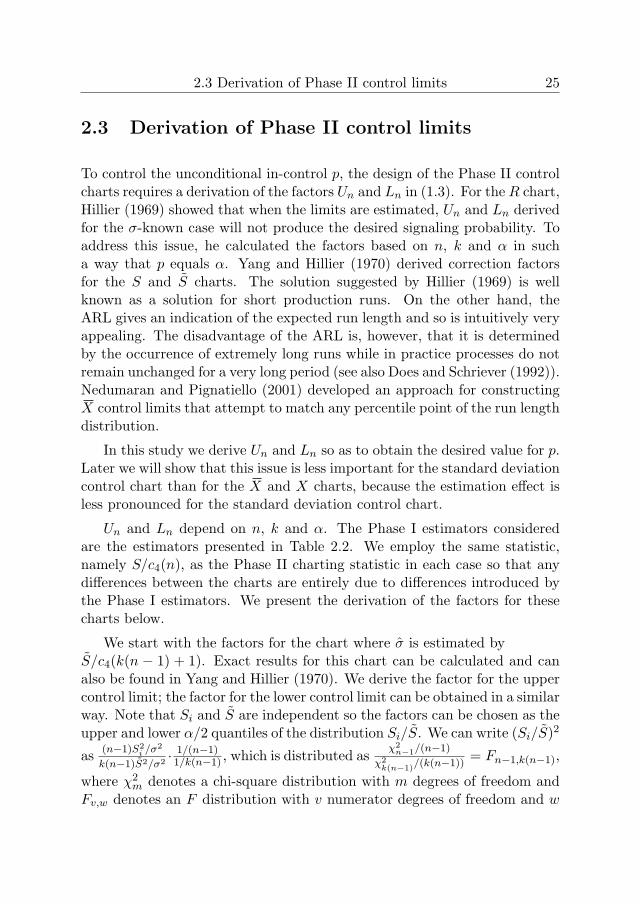
2.3 Derivation of Phase II control limits
To control the unconditional in-control p, the design of the Phase II controlcharts requires a derivation of the factors Un and Ln in (1.3). For the R chart,Hillier (1969) showed that when the limits are estimated, Un and Ln derivedfor the σ-known case will not produce the desired signaling probability. Toaddress this issue, he calculated the factors based on n, k and α in sucha way that p equals α. Yang and Hillier (1970) derived correction factorsfor the S and S charts. The solution suggested by Hillier (1969) is wellknown as a solution for short production runs. On the other hand, theARL gives an indication of the expected run length and so is intuitively veryappealing. The disadvantage of the ARL is, however, that it is determinedby the occurrence of extremely long runs while in practice processes do notremain unchanged for a very long period (see also Does and Schriever (1992)).Nedumaran and Pignatiello (2001) developed an approach for constructingX control limits that attempt to match any percentile point of the run lengthdistribution.
In this study we derive Un and Ln so as to obtain the desired value for p.Later we will show that this issue is less important for the standard deviationcontrol chart than for the X and X charts, because the estimation effect isless pronounced for the standard deviation control chart.
Un and Ln depend on n, k and α. The Phase I estimators consideredare the estimators presented in Table 2.2. We employ the same statistic,namely S/c4(n), as the Phase II charting statistic in each case so that anydifferences between the charts are entirely due to differences introduced bythe Phase I estimators. We present the derivation of the factors for thesecharts below.
We start with the factors for the chart where σ is estimated byS/c4(k(n − 1) + 1). Exact results for this chart can be calculated and canalso be found in Yang and Hillier (1970). We derive the factor for the uppercontrol limit; the factor for the lower control limit can be obtained in a similarway. Note that Si and S are independent so the factors can be chosen as theupper and lower α/2 quantiles of the distribution Si/S. We can write (Si/S)
2
as(n−1)S2
i /σ2
k(n−1)S2/σ2· 1/(n−1)1/k(n−1) , which is distributed as
χ2n−1/(n−1)
χ2k(n−1)
/(k(n−1)) = Fn−1,k(n−1),
where χ2m denotes a chi-square distribution with m degrees of freedom and
Fv,w denotes an F distribution with v numerator degrees of freedom and w

26 Standard Deviation Control Charts
denominator degrees of freedom. Hence
Un =
√Fn−1,k(n−1)(1− α/2)c4(k(n− 1) + 1)
c4(n). (2.12)
For the charts based on the other Phase I estimators we use the re-sult of Patnaik (1950). Patnaik approximated the distribution of R/σ bya(n, k)χν(n,k)/
√ν(n,k), where χν(n,k) is the square root of a chi-square dis-
tribution with ν(n, k) degrees of freedom and a(n, k) is a scale factor. Thefactors a(n, k) and ν(n, k) are obtained by equating the first two moments ofR/σ to the first two moments of a(n, k)χν(n,k)/
√ν(n,k). Patnaik’s approach
can also be applied to approximate the distribution of σ/σ, where σ is ob-tained via one of the unbiased estimators of the standard deviation in PhaseI. Let M1 = E(σ/σ) = 1 and M2 = V ar(σ/σ). From Patnaik (1950) itfollows that the values of ν(n, k) and a(n, k) are
ν(n, k) = 1/(−2 + 2√
1 + 2M2 + 1/(16ν(n, k))3), (2.13)
a(n, k) = 1 +1
4ν(n, k)+
1
32ν2(n, k)− 5
128ν3(n, k). (2.14)
Since (Si/σ)2
(c4(n)σ/σ)2is distributed as
χ2n−1/(n−1)
c24(n)a2(n,k)χ2
ν(n,k)/ν(n,k)
= Fn−1,ν(n,k)/(c24(n)a2(n, k)), it follows that
Un =√
F(n−1),ν(n,k)(1− α/2)/(c4(n)a(n, k)). (2.15)
Table 2.3 summarizes Un and Ln for the control charts with k = 20, 30, 75subgroups of sizes n = 5, 9 and α = 0.0027. For other situations, valuesof M2 can be derived by simulating σ/σ. Then the constants ν(n, k) anda(n, k) can be readily obtained from (2.13) and (2.14).
To judge the quality of the proposed corrections, we evaluate the un-conditional probabilities of a false signal (p) in Phase II. The probabilities,presented in Table 2.4, are assessed using 50,000 simulation runs. This isenough to obtain a sufficiently small relative standard error.
2.4 Control chart performance
In this section we evaluate the performance of the design schemes presentedabove. The schemes are set up in the uncontaminated normal situation and

2.4 Control chart performance 27
several contaminated situations. We consider models similar to those usedto assess the MSE with a, b and the multiplier equal to 4 to simulate thecontaminated cases (see Section 2.2.2).
The performance of the design schemes is assessed in terms of the un-conditional p and ARL as well as the conditional ARL associated with the2.5% and 97.5% quantiles of the distribution of σ. We consider differentshifts in the standard deviation λσ in Phase II, namely λ equal to 0.5, 1,1.5 and 2. The performance characteristics are obtained by simulation. Thenext section describes the simulation method, followed by the results forthe control charts constructed in the uncontaminated situation and variouscontaminated situations.
2.4.1 Simulation procedure
The performance characteristics p and ARL for estimated control limits aredetermined by averaging the conditional characteristics, i.e. the characteris-tics for a given set of estimated control limits, over all possible values of thecontrol limits. Recall the definitions of p(Fi|σ) from (1.5), E(RL|σ) from(1.6), p = E(p(Fi|σ)) from (1.7) and ARL = E( 1
p(Fi|σ)) from (1.8). Theseexpectations are obtained by simulation: 50,000 datasets are generated andfor each dataset p(Fi|σ) and E(RL|σ) are computed. By averaging thesevalues we obtain the unconditional values.
2.4.2 Simulation results
First we consider the situation where the process follows a normal distribu-tion and the Phase I data are not contaminated. We investigate the impactof the estimator used to estimate σ in Phase I. Tables 2.5 and 2.6 presentthe unconditional probability of one sample generating a signal (p), the un-conditional average run length (ARL) and the upper and lower conditionalARL values corresponding to the upper and lower 0.025 quantiles of thedistribution of σ. When λ = 1, the process is in control, so we want p tobe as low as possible and ARL to be as high as possible. When λ �= 1, i.e.in the out-of-control situation, we want to achieve the opposite. The tablesshow that, when the limits are estimated, the in-control ARL is higher thanthe desired 370 (the control limits are chosen to provide an unconditionalp of 0.0027), the value which is achieved when the limits are known. Notethat the increase in the unconditional ARL due to the estimation process

28 Standard Deviation Control Charts
is not as large as for the X control chart. The reason is that for the Xcontrol chart the run length distribution is very right-skewed, generating avery large unconditional ARL. This seems to be less the case for standarddeviation control charts.
We also study the conditional ARL values (or, equivalently, the condi-tional p values, since the conditional RL distribution is simply geometricwith parameter equal to the conditional p). The first value in parenthesesrepresents the ARL for the 2.5% quantile of the distribution of σ, while thesecond value represents the ARL for the 97.5% quantile of the distributionof σ. The results show that the conditional ARL values vary quite strongly,even when k equals 75. When λ equals 0.5, we see that a lower value of σgives a higher ARL and vice versa. The reason is that a smaller value of σ inPhase I results in a lower value for the lower control limit and hence a lowerprobability of detecting a decrease in the standard deviation in Phase II. Inthe normal uncontaminated situation, we observe a nice pattern for all theestimators: the upper and lower conditional ARL values in the in-control sit-uation are higher than in the out-of-control situation. However, this is notalways the case when there are Phase I contaminations (Tables 2.7-2.14).Confining ourselves to the conditional ARL values in the contaminated case,we judge the upper and lower conditional ARL values to be satisfactory,provided that they do not change too much from the values observed in theuncontaminated normal case.
When we compare the estimators in the uncontaminated Phase I situa-tion (Tables 2.5 and 2.6), S, S, R, G, ADM , ADM ′ and D7 produce verysimilar outcomes. The estimators S25, S20, IQR, MDM and MAD are lesspowerful under normality.
The performance of the charts in the case of contaminated data is tabu-lated in Tables 2.7-2.14. The same general results are found as for the MSEcomparisons. The most important points are as follows.
The chart based on S is most powerful under normality; however itsperformance decreases most quickly when diffuse or localized disturbancesoccur. In light of this risk, we do not recommend using S.
The charts based on the estimators S20, IQR and MDM perform rela-tively well in response to diffuse disturbances but not very well when thereare no contaminations.
Furthermore, the charts based on the estimatorsG andADM are efficientunder normality and are more efficient than the traditional charts based onS, S and R when diffuse outliers are present.
2.4 Control chart performance 29
Finally, the charts based on the estimators ADM ′ and D7 performequally well as the traditional charts in the uncontaminated case and sub-stantially better than any of the other charts in contaminated situations.When mean diffuse disturbances are likely to occur in Phase I, we recom-mend using D7 because the control chart based on this estimator is morerobust against such disturbances. When localized disturbances are likely tooccur, we recommend using ADM ′. Advantages of the latter estimator arethe ease of obtaining estimates and its intuitiveness: extreme samples, andhence the root cause of any disturbances, can be readily identified.

30 Standard Deviation Control Charts
Factors for control limitsk = 20 k = 30 k = 75
n σ Un Ln Un Ln Un Ln
5 S Eq. (2.12) 2.352 0.171 2.315 0.172 2.272 0.173S Eq. (2.15) 2.357 0.171 2.318 0.172 2.274 0.173S25 Eq. (2.15) 2.704 0.167 2.527 0.169 2.359 0.171S20 Eq. (2.15) 2.540 0.169 2.438 0.170 2.319 0.172R Eq. (2.15) 2.364 0.171 2.322 0.172 2.275 0.173IQR Eq. (2.15) 2.541 0.169 2.439 0.170 2.318 0.172G Eq. (2.15) 2.359 0.171 2.320 0.172 2.275 0.173ADM Eq. (2.15) 2.366 0.171 2.324 0.172 2.275 0.173ADM ′ Eq. (2.15) 2.376 0.171 2.332 0.171 2.279 0.172MDM Eq. (2.15) 2.554 0.169 2.442 0.170 2.322 0.172MAD Eq. (2.15) 2.447 0.170 2.380 0.171 2.296 0.172D7 Eq. (2.15) 2.376 0.171 2.331 0.172 2.278 0.172
9 S Eq. (2.12) 1.890 0.349 1.872 0.350 1.851 0.351S Eq. (2.15) 1.892 0.349 1.873 0.350 1.852 0.351S25 Eq. (2.15) 2.011 0.342 1.946 0.345 1.883 0.349S20 Eq. (2.15) 1.987 0.343 1.934 0.346 1.876 0.349R Eq. (2.15) 1.900 0.348 1.879 0.349 1.854 0.351IQR Eq. (2.15) 1.982 0.343 1.933 0.346 1.875 0.350G Eq. (2.15) 1.894 0.348 1.874 0.350 1.852 0.351ADM Eq. (2.15) 1.898 0.348 1.877 0.349 1.854 0.351ADM ′ Eq. (2.15) 1.901 0.348 1.879 0.349 1.854 0.351MDM Eq. (2.15) 1.987 0.343 1.936 0.346 1.876 0.349MAD Eq. (2.15) 1.956 0.345 1.915 0.347 1.868 0.350D7 Eq. (2.15) 1.901 0.348 1.879 0.349 1.854 0.351
Table 2.3: Factors Un and Ln to determine Phase II control limits

2.4 Control chart performance 31
p× 102
k = 20 k = 30 k = 75n σ Un Ln Un Ln Un Ln
5 S Eq. (2.12) 0.135 0.135 0.135 0.135 0.135 0.135S Eq. (2.15) 0.135 0.135 0.135 0.135 0.135 0.135S25 Eq. (2.15) 0.131 0.134 0.135 0.135 0.135 0.134S20 Eq. (2.15) 0.135 0.135 0.135 0.134 0.136 0.135R Eq. (2.15) 0.135 0.134 0.135 0.136 0.135 0.137IQR Eq. (2.15) 0.130 0.134 0.131 0.134 0.135 0.135G Eq. (2.15) 0.133 0.134 0.136 0.135 0.134 0.136ADM Eq. (2.15) 0.132 0.134 0.135 0.135 0.134 0.137ADM ′ Eq. (2.15) 0.136 0.135 0.137 0.133 0.134 0.134MDM Eq. (2.15) 0.130 0.136 0.133 0.134 0.134 0.136MAD Eq. (2.15) 0.131 0.135 0.130 0.135 0.134 0.135D7 Eq. (2.15) 0.135 0.135 0.134 0.136 0.136 0.133
9 S Eq. (2.12) 0.134 0.135 0.134 0.135 0.134 0.135S Eq. (2.15) 0.136 0.134 0.136 0.136 0.134 0.135S25 Eq. (2.15) 0.141 0.135 0.137 0.134 0.134 0.135S20 Eq. (2.15) 0.131 0.134 0.135 0.135 0.135 0.133R Eq. (2.15) 0.135 0.135 0.134 0.134 0.134 0.136IQR Eq. (2.15) 0.134 0.134 0.133 0.135 0.133 0.137G Eq. (2.15) 0.133 0.134 0.134 0.136 0.134 0.136ADM Eq. (2.15) 0.134 0.135 0.134 0.134 0.133 0.136ADM ′ Eq. (2.15) 0.134 0.135 0.138 0.134 0.135 0.135MDM Eq. (2.15) 0.134 0.134 0.138 0.134 0.136 0.133MAD Eq. (2.15) 0.134 0.136 0.133 0.135 0.133 0.136D7 Eq. (2.15) 0.134 0.135 0.136 0.134 0.133 0.136
Table 2.4: In-control p × 102 of control limits. The estimated relative stan-dard error is never worse than 1%

32 Standard Deviation Control Charts
p ARLk σ λ = 0.5 λ = 1 λ = 1.5 λ = 2 λ = 0.5 λ = 1 λ = 1.5 λ = 2
30 S 0.019 0.0027 0.084 0.32 54.7 418 14.5 3.28(86.7; 33.7) (151; 455) (5.94; 33.0) (2.18; 5.10)
S 0.019 0.0027 0.083 0.32 54.7 419 14.8 3.30(87.8; 33.4) (150; 451) (5.90; 34.2) (2.18; 5.18)
S25 0.019 0.0027 0.058 0.25 65.1 535 47.8 5.45(155; 24.7) (91.9; 334) (4.78; 248) (1.95; 15.2)
S20 0.019 0.0027 0.068 0.27 60.9 490 28.3 4.29(126; 27.1) (104; 369) (5.03; 113) (2.01; 9.63)
R 0.019 0.0027 0.082 0.32 54.9 421 15.1 3.33(88.8; 32.9) (147; 447) (5.85; 35.9) (2.17; 5.31)
IQR 0.019 0.0026 0.067 0.27 61.0 490 28.5 4.32(125; 27.0) (106; 367) (5.06; 114) (2.01; 9.66)
G 0.019 0.0027 0.083 0.32 54.8 421 14.9 3.52(88.3; 33.2) (148; 450) (5.87; 35.1) (2.17; 5.53)
ADM 0.020 0.0027 0.082 0.32 54.8 423 15.2 3.34(89.1; 32.8) (148; 444) (5.87; 36.6) (2.16; 5.34)
ADM ′ 0.019 0.0027 0.081 0.31 56.5 434 15.7 3.39(95.2; 33.2) (138; 451) (5.69; 39.3) (2.13; 5.50)
MDM 0.019 0.0027 0.067 0.27 60.9 490 29.2 4.37(129; 26.6) (101; 365) (5.02; 123) (2.01; 10.0)
MAD 0.019 0.0026 0.074 0.29 57.7 457 20.4 3.77(107; 29.4) (124; 404) (5.40; 65.6) (2.08; 7.20)
D7 0.020 0.0027 0.081 0.31 55.1 427 15.7 3.38(92.0; 32.4) (140; 442) (5.72; 38.7) (2.14; 5.49)
75 S 0.019 0.0027 0.090 0.34 52.7 391 11.9 3.02(70.8; 38.8) (208; 479) (6.98; 19.8) (2.35; 3.92)
S 0.020 0.0027 0.090 0.34 52.7 392 12.0 3.03(71.2; 38.6) (205; 478) (6.94; 20.1) (2.35; 3.94)
S25 0.019 0.0027 0.077 0.30 57.1 446 18.2 3.60(101; 30.8) (127; 423) (5.24; 52.5) (2.10; 6.44)
S20 0.019 0.0027 0.083 0.32 54.8 420 14.8 3.30(88.2; 33.2) (150; 451) (5.90; 34.7) (2.17; 5.20)
R 0.020 0.0027 0.090 0.34 52.3 391 12.1 3.05(71.1; 38.0) (203; 475) (6.88; 20.6) (2.34; 4.00)
IQR 0.020 0.0027 0.083 0.32 54.7 419 14.8 3.30(88.0; 33.1) (150; 450) (5.90; 34.6) (2.17; 5.20)
G 0.020 0.0027 0.090 0.34 52.2 391 12.0 3.04(70.8; 38.1) (206; 476) (6.93; 20.4) (2.35; 3.98)
ADM 0.020 0.0027 0.090 0.34 52.2 391 12.1 3.04(71.4; 37.8) (201; 474) (6.87; 20.7) (2.34; 4.00)
ADM ′ 0.019 0.0027 0.089 0.33 53.4 399 12.3 3.07(74.4; 38.2) (194; 484) (6.74; 21.6) (2.32; 4.09)
MDM 0.020 0.0027 0.082 0.32 54.7 422 15.0 3.33(88.0; 32.8) (150; 449) (5.89; 36.1) (2.17; 5.29)
MAD 0.019 0.0027 0.086 0.33 53.9 409 13.3 3.17(80.2; 35.4) (174; 471) (6.29; 27.2) (2.25; 4.59)
D7 0.019 0.0027 0.090 0.34 53.6 396 12.1 3.04(74.1; 38.5) (197; 485) (6.75; 21.1) (2.32; 4.06)
Table 2.5: Unconditional p and ARL and (in parentheses) the upper andlower conditional ARL values under normality for n = 5

2.4 Control chart performance 33
p ARLk σ λ = 0.5 λ = 1 λ = 1.5 λ = 2 λ = 0.5 λ = 1 λ = 1.5 λ = 2
30 S 0.12 0.0027 0.17 0.58 9.05 402 6.48 1.74(14.4; 5.64) (173; 394) (3.52; 11.9) (1.42; 2.22)
S 0.12 0.0027 0.17 0.58 9.02 400 6.52 1.75(14.4; 5.57) (172; 390) (3.50; 12.1) (1.42; 2.23)
S25 0.11 0.0027 0.14 0.52 10.6 479 10.4 2.02(24.2; 4.52) (108; 296) (2.97; 32.3) (1.34; 3.35)
S20 0.11 0.0027 0.15 0.53 10.3 462 9.60 1.96(22.3; 4.59) (119; 306) (3.05; 28.4) (1.35; 3.15)
R 0.12 0.0027 0.17 0.58 9.23 410 6.74 1.77(15.1; 5.48) (163; 383) (3.44; 13.3) (1.42; 2.31)
IQR 0.11 0.0027 0.15 0.54 10.3 463 9.52 1.96(22.0; 4.59) (118; 306) (3.06; 28.0) (1.35; 3.13)
G 0.12 0.0027 0.17 0.58 9.02 401 6.55 1.75(14.5; 5.56) (171; 387) (3.50; 12.2) (1.41; 2.25)
ADM 0.12 0.0027 0.17 0.58 9.17 409 6.69 1.76(15.1; 5.51) (168; 387) (3.46; 13.0) (1.41; 2.29)
ADM ′ 0.12 0.0027 0.17 0.58 9.22 409 6.75 1.77(15.4; 5.49) (160; 385) (3.40; 13.1) (1.40; 2.32)
MDM 0.11 0.0027 0.14 0.53 10.4 465 9.68 1.97(22.5; 4.59) (115; 300) (3.03; 29.0) (1.35; 3.18)
MAD 0.12 0.0027 0.15 0.55 9.90 444 8.48 1.89(19.7; 4.82) (130; 325) (3.13; 22.0) (1.37; 2.85)
D7 0.12 0.0027 0.17 0.58 9.22 410 6.73 1.76(15.3; 5.50) (165; 385) (3.43; 13.1) (1.40; 2.32)
75 S 0.12 0.0027 0.18 0.60 8.67 383 5.77 1.68(11.7; 6.43) (235; 429) (3.97; 8.39) (1.48; 1.94)
S 0.12 0.0027 0.18 0.60 8.67 383 5.78 1.68(11.7; 6.39) (229; 429) (3.96; 8.45) (1.48; 1.94)
S25 0.12 0.0027 0.17 0.57 9.27 412 6.90 1.78(15.8; 5.42) (156; 380) (3.38; 13.9) (1.40; 2.36)
S20 0.12 0.0027 0.17 0.58 9.22 408 6.58 1.75(15.0; 5.58) (169; 394) (3.46; 12.4) (1.41; 2.26)
R 0.12 0.0027 0.18 0.60 8.70 384 5.85 1.69(12.0; 6.26) (225; 425) (3.90; 8.86) (1.47; 1.98)
IQR 0.12 0.0027 0.17 0.58 9.02 402 6.58 1.75(14.6; 5.52) (196; 386) (3.48; 12.4) (1.41; 2.26)
G 0.12 0.0027 0.18 0.60 8.68 384 5.80 1.68(11.7; 6.38) (231; 428) (3.95; 8.53) (1.48; 1.95)
ADM 0.12 0.0027 0.18 0.59 8.67 386 5.86 1.69(11.9; 6.28) (225; 427) (3.95; 8.78) (1.47; 1.97)
ADM ′ 0.12 0.0027 0.18 0.60 8.70 384 5.86 1.69(12.0; 6.28) (219; 425) (3.87; 8.84) (1.46; 1.98)
MDM 0.12 0.0027 0.17 0.58 9.23 407 6.58 1.75(95.2; 33.2) (138; 451) (5.69; 39.3) (2.13; 5.50)
MAD 0.12 0.0027 0.17 0.58 8.96 398 6.35 1.73(13.9; 5.73) (185; 401) (3.60; 11.2) (1.43; 2.18)
D7 0.12 0.0027 0.18 0.60 8.69 385 5.84 1.70(12.0; 6.28) (223; 426) (3.89; 8.81) (1.46; 1.98)
Table 2.6: Unconditional p and ARL and (in parentheses) the upper andlower conditional ARL values under normality for n = 9

34 Standard Deviation Control Charts
p ARLk σ λ = 0.5 λ = 1 λ = 1.5 λ = 2 λ = 0.5 λ = 1 λ = 1.5 λ = 2
30 S 0.055 0.0043 0.016 0.11 23.0 293 195 22.9(52.0; 7.68) (475; 92.0) (13.2; 427) (3.22; 131)
S 0.041 0.0031 0.024 0.15 28.7 359 104 9.45(55.8; 12.5) (441; 158) (11.5; 468) (3.02; 30.8)
S25 0.024 0.0024 0.040 0.20 52.7 526 84.4 7.60(128; 19.4) (164; 262) (6.00; 478) (2.19; 24.7)
S20 0.024 0.0023 0.045 0.22 48.5 493 54.9 5.97(103; 20.4) (187; 275) (6.50; 272) (2.29; 16.6)
R 0.041 0.0032 0.023 0.15 28.4 356 110 9.82(55.4; 12.2) (445; 157) (11.8; 483) (3.05; 32.7)
IQR 0.024 0.0023 0.044 0.22 48.3 493 55.0 5.99(103; 20.4) (191; 276) (6.56; 274) (2.29; 16.2)
G 0.038 0.0029 0.026 0.16 30.2 379 86.0 8.10(56.6; 14.0) (429; 183) (11.3; 388) (2.99; 23.3)
ADM 0.035 0.0027 0.029 0.17 31.8 393 73.2 7.28(58.9; 15.3) (411; 200) (10.8; 320) (2.92; 19.3)
ADM ′ 0.024 0.0025 0.060 0.26 47.2 450 27.0 4.31(86.6; 24.0) (178; 330) (6.41; 94.1) (2.25; 8.80)
MDM 0.026 0.0023 0.041 0.21 46.6 489 63.5 6.43(99.6; 19.3) (213; 259) (6.89; 323) (2.35; 18.4)
MAD 0.033 0.0026 0.029 0.17 34.9 423 86.3 8.02(69.6; 15.6) (382; 206) (9.68; 412) (2.78; 23.8)
D7 0.025 0.0024 0.055 0.25 44.1 452 27.8 4.41(76.6; 23.9) (230; 326) (7.30; 90.8) (2.40; 8.50)
75 S 0.054 0.0042 0.012 0.11 20.4 270 163 13.5(36.1; 10.3) (467; 128) (23.0; 478) (4.23; 42.5)
S 0.040 0.0030 0.022 0.16 26.7 353 68.3 7.86(41.7; 16.0) (482; 210) (17.3; 217) (3.67; 14.8)
S25 0.024 0.0023 0.053 0.25 46.4 473 29.4 4.55(83.1; 24.7) (219; 339) (7.04; 97.3) (2.38; 9.01)
S20 0.025 0.0023 0.054 0.25 43.3 459 25.1 4.25(27.4; 25.6) (276; 351) (8.08; 68.7) (2.52; 7.49)
R 0.041 0.0030 0.022 0.16 26.2 347 70.5 7.30(41.2; 15.7) (478; 205) (17.5; 226) (3.69; 15.2)
IQR 0.025 0.0023 0.054 0.25 43.2 459 25.0 4.25(70.1; 25.7) (276; 351) (8.07; 96.0) (2.52; 7.48)
G 0.037 0.0028 0.026 0.17 28.1 371 55.2 6.41(42.7; 17.6) (477; 233) (16.2; 161) (3.53; 12.2)
ADM 0.035 0.0027 0.029 0.18 29.7 387 46.9 5.89(44.5; 18.9) (470; 253) (15.1; 128) (3.41; 10.6)
ADM ′ 0.023 0.0023 0.065 0.28 44.7 445 18.2 3.69(65.9; 29.5) (269; 403) (8.00; 39.3) (2.52; 5.56)
MDM 0.026 0.0023 0.049 0.24 41.5 458 28.4 4.51(67.8; 24.3) (299; 332) (8.57; 80.6) (2.59; 8.12)
MAD 0.033 0.0025 0.031 0.19 32.2 413 45.8 5.78(50.7; 20.0) (462; 264) (13.0; 135) (3.18; 10.9)
D7 0.024 0.0022 0.059 0.27 42.7 454 19.5 3.82(61.1; 29.2) (321; 399) (9.05; 40.3) (2.66; 5.61)
Table 2.7: Unconditional p and ARL and (in parentheses) the upper andlower conditional ARL values when symmetric variance disturbances arepresent in Phase I for n = 5

2.4 Control chart performance 35
p ARLk σ λ = 0.5 λ = 1 λ = 1.5 λ = 2 λ = 0.5 λ = 1 λ = 1.5 λ = 2
30 S 0.40 0.011 0.021 0.21 2.91 147 156 8.78(6.13; 1.41) (432; 39.2) (10.2; 417) (2.10; 36.4)
S 0.32 0.0068 0.033 0.27 3.55 200 77.4 4.61(6.77; 1.81) (463; 55.6) (8.73; 384) (1.98; 12.3)
S25 0.16 0.0026 0.089 0.43 7.70 449 20.9 2.58(17.6; 3.31) (242; 197) (3.93; 83.7) (1.47; 5.03)
S20 0.15 0.0025 0.10 0.46 7.92 456 15.8 2.35(16.7; 3.63) (233; 207) (3.88; 54.6) (1.47; 4.18)
R 0.35 0.0084 0.025 0.23 3.24 175 118 6.19(6.52; 1.60) (461; 41.8) (9.69; 494) (2.05; 20.4)
IQR 0.15 0.0025 0.10 0.46 7.79 454 15.9 2.35(16.5; 3.62) (240; 205) (3.93; 55.3) (1.47; 4.19)
G 0.27 0.0050 0.045 0.32 4.08 246 43.2 3.52(7.38; 2.20) (480; 84.8) (7.69; 181) (1.87; 7.45)
ADM 0.24 0.0042 0.054 0.35 4.56 284 31.2 3.09(8.11; 2.52) (490; 110) (7.03; 114) (1.82; 5.85)
ADM ′ 0.16 0.0027 0.12 0.49 7.10 400 11.5 2.12(13.2; 3.72) (236; 217) (3.95; 31.7) (1.48; 3.32)
MDM 0.15 0.0025 0.096 0.45 7.73 452 17.0 2.41(16.5; 3.52) (249; 197) (3.96; 59.8) (1.48; 4.36)
MAD 0.18 0.0029 0.076 0.41 6.21 392 22.0 2.66(12.3; 3.07) (392; 156) (4.92; 80.3) (1.59; 4.91)
D7 0.15 0.0025 0.11 0.49 7.02 415 10.8 2.09(12.0; 4.03) (294; 247) (4.32; 25.9) (1.53; 3.05)
75 S 0.41 0.010 0.016 0.20 2.61 121 123 6.10(4.23; 1.65) (262; 44.7) (18.4; 414) (2.65; 15.2)
S 0.32 0.0063 0.030 0.28 3.30 180 49.4 3.85(5.00; 2.15) (336; 82.0) (13.1; 157) (3.31; 7.00)
S25 0.16 0.0025 0.11 0.48 6.72 414 11.7 2.15(11.4; 3.95) (331; 241) (4.62; 27.9) (1.56; 3.12)
S20 0.15 0.0024 0.12 0.50 7.06 426 9.90 2.04(11.3; 4.36) (320; 279) (4.56; 20.9) (1.56; 2.79)
R 0.36 0.0079 0.022 0.24 2.96 149 77.3 4.71(4.60; 1.90) (301; 62.6) (15.6; 274) (2.46; 9.68)
IQR 0.15 0.0025 0.12 0.50 6.90 417 10.0 2.04(11.0; 4.27) (324; 271) (4.59; 21.0) (1.56; 2.80)
G 0.27 0.0048 0.044 0.34 3.83 229 29.3 3.11(5.59; 2.59) (383; 118) (10.5; 74.7) (2.12; 4.86)
ADM 0.24 0.0041 0.055 0.37 4.25 266 22.1 2.80(6.10; 2.93) (417; 146) (9.23; 50.4) (2.02; 4.07)
ADM ′ 0.16 0.0025 0.12 0.52 6.64 401 8.99 1.97(9.82; 4.44) (331; 287) (4.75; 16.8) (1.58; 2.54)
MDM 0.15 0.0025 0.11 0.49 6.88 422 10.4 2.07(8.66; 3.61) (443; 207) (6.00; 30.7) (1.71; 3.28)
MAD 0.19 0.0029 0.086 0.44 5.60 368 13.9 2.32(95.2; 33.2) (138; 451) (5.69; 39.3) (2.13; 5.50)
D7 0.16 0.0025 0.12 0.51 6.58 409 8.85 1.97(9.22; 4.65) (370; 307) (5.15; 15.2) (1.66; 2.44)
Table 2.8: Unconditional p and ARL and (in parentheses) the upper andlower conditional ARL values when symmetric variance disturbances arepresent in Phase I for n = 9

36 Standard Deviation Control Charts
p ARLk σ λ = 0.5 λ = 1 λ = 1.5 λ = 2 λ = 0.5 λ = 1 λ = 1.5 λ = 2
30 S 0.16 0.020 0.016 0.074 16.1 189 211 137(54.9; 1.46) (444; 8.54) (12.0; 34.0) (3.08; 99.9)
S 0.063 0.0052 0.019 0.12 23.6 286 196 43.3(57.8; 5.15) (420; 56.2) (11.1; 262) (2.95; 447)
S25 0.023 0.0024 0.044 0.21 55.1 530 74.8 7.08(133; 20.5) (140; 279) (5.79; 421) (2.13; 22.8)
S20 0.025 0.0024 0.047 0.22 49.6 488 57.9 6.88(106; 19.0) (173; 249) (6.30; 354) (2.24; 20.2)
R 0.061 0.0050 0.019 0.12 23.8 291 195 39.5(52.3; 5.51) (420; 61.2) (11.1; 284) (2.95; 389)
IQR 0.025 0.0024 0.047 0.22 49.5 490 58.3 6.72(107; 19.1) (176; 254) (6.36; 339) (2.24; 19.6)
G 0.053 0.0042 0.021 0.13 25.8 315 168 25.6(58.2; 6.94) (407; 80.3) (10.8; 375) (2.91; 195)
ADM 0.047 0.0037 0.023 0.14 27.6 334 147 18.8(60.0; 8.23) (403; 98.5) (10.5; 458) (2.88; 113)
ADM ′ 0.022 0.0025 0.069 0.28 51.1 448 21.0 3.86(90.7; 27.5) (153; 378) (5.94; 63.3) (2.19; 7.12)
MDM 0.024 0.0023 0.045 0.22 48.8 492 56.0 6.05(104; 20.5) (181; 275) (6.48; 279) (2.25; 16.8)
MAD 0.046 0.0037 0.022 0.13 29.4 352 176 23.9(68.9; 8.06) (405; 96.4) (9.89; 453) (2.79; 166)
D7 0.023 0.0024 0.062 0.27 47.5 452 22.6 4.00(81.3; 26.5) (197; 363) (6.71; 65.1) (2.32; 7.24)
75 S 0.16 0.017 0.0079 0.038 10.5 130 263 163(32.5; 1.91) (432; 13.9) (31.1; 61.8) (4.88; 185)
S 0.059 0.0046 0.013 0.11 20.2 264 186 19.7(39.5; 7.93) (482; 93.3) (19.1; 427) (3.85; 95.0)
S25 0.023 0.0023 0.057 0.26 48.5 473 26.7 4.31(86.8; 25.9) (198; 343) (6.71; 83.8) (2.31; 8.27)
S20 0.025 0.0023 0.056 0.26 44.0 453 26.2 4.27(72.8; 24.0) (256; 328) (7.64; 84.5) (2.47; 8.15)
R 0.058 0.0045 0.013 0.11 20.4 268 177 17.6(39.4; 8.24) (478; 99.1) (19.2; 449) (3.87; 78.1)
IQR 0.025 0.0023 0.056 0.26 44.0 453 25.7 4.27(72.7; 24.2) (256; 332) (7.66; 81.3) (2.47; 8.02)
G 0.050 0.0038 0.016 0.13 22.7 299 135 12.1(41.2; 10.1) (480; 124) (17.5; 478) (3.70; 43.3)
ADM 0.046 0.0035 0.019 0.14 24.5 320 107 9.66(42.9; 11.7) (477; 147) (16.2; 433) (3.54; 29.6)
ADM ′ 0.021 0.0024 0.075 0.30 48.4 433 15.3 3.39(70.0; 32.9) (231; 442) (7.42; 30.2) (2.42; 4.82)
MDM 0.025 0.0023 0.054 0.25 43.5 460 25.4 4.25(71.6; 25.5) (268; 349) (8.00; 72.2) (2.52; 7.53)
MAD 0.044 0.0034 0.019 0.14 25.7 335 116 10.2(47.0; 11.7) (492; 147) (15.1; 472) (3.42; 33.0)
D7 0.022 0.0023 0.069 0.29 46.1 447 16.4 3.52(64.8; 32.2) (278; 433) (8.21; 31.9) (2.55; 4.97)
Table 2.9: Unconditional p and ARL and (in parentheses) the upper andlower conditional ARL values when asymmetric variance disturbances arepresent in Phase I for n = 5

2.4 Control chart performance 37
p ARLk σ λ = 0.5 λ = 1 λ = 1.5 λ = 2 λ = 0.5 λ = 1 λ = 1.5 λ = 2
30 S 0.69 0.11 0.025 0.093 1.90 68.9 176 122(5.92; 1.00) (412; 1.63) (10.9; 8.33) (2.14; 44.3)
S 0.48 0.021 0.021 0.17 2.66 127 192 33.7(6.68; 1.09) (460; 9.89) (8.81; 123) (1.97; 383)
S25 0.15 0.0026 0.099 0.45 8.20 462 17.7 2.43(18.6; 3.52) (208; 198) (3.67; 66.8) (1.44; 4.60)
S20 0.14 0.0025 0.11 0.47 8.28 460 14.9 2.29(17.7; 3.63) (204; 217) (3.69; 51.7) (1.44; 4.06)
R 0.50 0.024 0.017 0.15 2.52 116 214 43.3(6.45; 1.07) (453; 8.73) (9.72; 107) (2.06; 469)
IQR 0.14 0.0025 0.11 0.47 8.18 459 15.0 2.29(17.4; 3.68) (211; 268) (3.71; 51.7) (1.45; 4.05)
G 0.37 0.010 0.030 0.24 3.31 179 126 8.78(7.26; 1.37) (478; 26.5) (7.77; 390) (1.89; 41.9)
ADM 0.31 0.0070 0.038 0.28 3.81 220 87.5 5.42(7.95; 1.63) (491; 42.4) (7.10; 490) (1.82; 19.6)
ADM ′ 0.14 0.0026 0.14 0.53 7.95 413 9.00 1.95(14.4; 4.34) (190; 277) (3.67; 21.6) (1.43; 2.83)
MDM 0.14 0.0025 0.10 0.47 8.16 461 15.3 2.31(17.2; 3.68) (220; 216) (3.77; 52.3) (1.45; 4.08)
MAD 0.26 0.0052 0.049 0.32 4.79 291 74.2 4.73(10.8; 1.82) (479; 56.1) (5.68; 517) (1.67; 16.2)
D7 0.14 0.0025 0.13 0.52 7.69 426 9.07 1.96(12.9; 4.46) (249; 291) (4.02; 20.3) (1.48; 2.74)
75 S 0.77 0.092 0.012 0.044 1.42 32.1 205 145(2.95; 1.00) (150; 2.59) (46.5; 18.5) (3.97; 111)
S 0.49 0.017 0.012 0.15 2.27 94.3 204 14.3(4.26; 1.25) (269; 19.3) (18.3; 272) (2.63; 71.1)
S25 0.15 0.0025 0.12 0.50 7.18 424 10.4 2.06(12.1; 4.21) (288; 266) (4.31; 23.8) (1.52; 2.92)
S20 0.14 0.0024 0.13 0.52 7.36 429 9.33 1.99(12.0; 4.47) (292; 293) (4.33; 19.8) (1.52; 2.72)
R 0.52 0.019 0.0093 0.13 2.11 82.0 233 18.6(3.93; 1.20) (241; 16.9) (21.7; 233) (2.86; 102)
IQR 0.15 0.0025 0.12 0.51 7.20 420 9.28 1.99(11.6; 4.40) (294; 284) (4.36; 19.9) (1.53; 2.73)
G 0.37 0.0086 0.024 0.24 2.97 151 92.8 5.25(5.03; 1.68) (342; 46.9) (12.7; 395) (2.29; 14.1)
ADM 0.31 0.0064 0.034 0.29 3.41 191 54.7 3.95(5.58; 1.99) (385; 69.3) (10.7; 226) (2.13; 8.53)
ADM ′ 0.14 0.0025 0.15 0.55 7.47 408 7.39 1.83(10.8; 5.11) (277; 347) (4.32; 12.7) (1.52; 2.27)
MDM 0.15 0.0024 0.12 0.51 7.25 428 9.50 2.00(11.8; 4.47) (297; 288) (4.38; 20.1) (1.53; 2.72)
MAD 0.26 0.0047 0.059 0.34 4.19 256 36.3 3.29(7.21; 2.29) (470; 92.0) (7.70; 143) (1.88; 6.71)
D7 0.14 0.0024 0.14 0.54 7.22 416 7.63 1.86(10.0; 5.17) (321; 351) (4.70; 12.4) (1.56; 2.26)
Table 2.10: Unconditional p and ARL and (in parentheses) the upper andlower conditional ARL values when asymmetric variance disturbances arepresent in Phase I for n = 9

38 Standard Deviation Control Charts
p ARLk σ λ = 0.5 λ = 1 λ = 1.5 λ = 2 λ = 0.5 λ = 1 λ = 1.5 λ = 2
30 S 0.10 0.0083 0.0038 0.035 12.1 153 370 92.9(26.3; 4.82) (362; 51.7) (63.6; 243) (7.10; 476)
S 0.051 0.0038 0.011 0.10 21.3 286 172 13.1(36.8; 12.0) (489; 152) (27.0; 486) (4.58; 34.6)
S25 0.022 0.0024 0.047 0.22 57.2 534 66.1 6.47(136; 21.8) (129; 291) (5.54; 363) (2.09; 19.6)
S20 0.051 0.0039 0.010 0.086 24.3 317 285 27.4(54.9; 9.42) (633; 115) (18.4; 540) (3.77; 133)
R 0.051 0.0038 0.011 0.10 21.4 286 176 12.2(37.3; 11.8) (492; 150) (27.0; 499) (4.59; 36.4)
IQR 0.051 0.0039 0.010 0.086 24.3 316 286 28.1(55.0; 9.39) (633; 115) (18.4; 537) (3.78; 134)
G 0.051 0.0038 0.011 0.10 21.4 286 174 13.1(37.1; 11.9) (450; 151) (27.1; 491) (4.62; 35.2)
ADM 0.051 0.0038 0.010 0.099 21.4 287 178 13.5(37.1; 11.7) (496; 149) (26.4; 503) (4.55; 37.2)
ADM ′ 0.020 0.0027 0.079 0.31 55.1 433 17.3 3.53(97.2; 30.3) (130; 415) (5.51; 48.1) (2.11; 6.16)
MDM 0.051 0.0039 0.010 0.086 24.3 318 288 28.7(56.0; 9.25) (635; 112) (18.1; 532) (3.75; 144)
MAD 0.051 0.0039 0.010 0.092 22.7 301 233 18.9(46.0; 10.3) (573; 128) (21.7; 563) (4.09; 72.3)
D7 0.025 0.0023 0.053 0.25 43.6 454 27.9 4.43(75.6; 24.2) (240; 327) (7.34; 85.2) (2.44; 8.44)
75 S 0.080 0.0064 0.0041 0.050 13.5 175 330 32.9(22.9; 7.39) (312; 87.4) (73.0; 406) (7.74; 117)
S 0.043 0.0032 0.017 0.14 24.1 326 77.6 7.77(34.2; 16.7) (450; 222) (26.7; 186) (4.57; 13.3)
S25 0.021 0.0024 0.065 0.28 51.7 467 22.5 3.99(92.7; 27.8) (165; 384) (6.21; 67.9) (2.21; 7.39)
S20 0.043 0.0032 0.016 0.13 25.3 337 112 9.48(43.1; 14.1) (520; 183) (19.4; 377) (3.85; 23.0)
R 0.043 0.0032 0.017 0.14 24.0 323 78.1 7.81(33.9; 16.5) (448; 218) (26.1; 188) (4.53; 13.6)
IQR 0.043 0.0032 0.016 0.13 0.043 337 112 9.51(43.0; 14.1) (519; 183) (19.3; 375) (3.85; 23.1)
G 0.043 0.0032 0.017 0.14 23.9 323 77.6 7.82(33.7; 16.6) (447; 220) (26.5; 186) (4.55; 13.5)
ADM 0.043 0.0032 0.017 0.14 23.9 323 78.9 7.84(34.3; 16.4) (449; 217) (26.2; 195) (4.52; 13.7)
ADM ′ 0.020 0.0026 0.087 0.33 52.4 405 12.8 3.13(74.6; 36.5) (194; 474) (6.72; 23.7) (2.31; 4.30)
MDM 0.043 0.0032 0.016 0.13 25.2 336 115 9.69(43.3; 14.0) (522; 180) (19.3; 392) (3.85; 24.1)
MAD 0.043 0.0032 0.016 0.13 24.8 333 94.4 8.60(38.7; 15.3) (494; 139) (22.1; 288) (4.13; 18.0)
D7 0.023 0.0023 0.064 0.28 44.7 452 17.5 3.63(63.1; 31.1) (295; 423) (8.55; 34.2) (2.60; 5.19)
Table 2.11: Unconditional p and ARL and (in parentheses) the upperand lower conditional ARL values when localized variance disturbances arepresent in Phase I for n = 5

2.4 Control chart performance 39
p ARLk σ λ = 0.5 λ = 1 λ = 1.5 λ = 2 λ = 0.5 λ = 1 λ = 1.5 λ = 2
30 S 0.66 0.033 0.0037 0.054 1.60 43.1 344 49.3(2.60; 1.12) (117; 12.0) (93.7; 154) (5.30; 263)
S 0.38 0.0088 0.015 0.20 2.75 132 111 5.63(4.22; 1.86) (462; 59.3) (21.8; 346) (2.82; 11.4)
S25 0.13 0.0025 0.12 0.49 9.49 481 12.8 2.17(21.5; 4.13) (142; 255) (3.24; 41.9) (1.38; 3.74)
S20 0.37 0.0089 0.015 0.18 3.09 164 201 8.68(6.29; 1.61) (469; 42.3) (14.2; 590) (2.40; 30.0)
R 0.38 0.0087 0.015 0.20 2.80 136 120 5.86(4.41; 1.82) (285; 57.5) (20.9; 395) (2.77; 12.7)
IQR 0.37 0.0089 0.014 0.18 3.09 162 202 8.59(6.25; 1.61) (467; 42.3) (14.5; 591) (2.42; 29.2)
G 0.38 0.0088 0.015 0.20 2.75 133 113 5.68(4.23; 1.85) (269; 59.4) (21.7; 358) (2.82; 11.7)
ADM 0.38 0.0087 0.015 0.20 2.79 135 117 5.79(4.37; 1.84) (276; 58.0) (21.1; 379) (2.79; 12.2)
ADM ′ 0.12 0.0028 0.17 0.57 9.21 405 6.86 1.78(15.9; 5.33) (147; 369) (3.31; 14.0) (1.39; 2.37)
MDM 0.37 0.0089 0.015 0.18 3.10 164 203 8.78(6.27; 1.61) (475; 42.2) (14.4; 587) (2.39; 30.6)
MAD 0.37 0.0088 0.015 0.18 2.97 154 175 7.54(5.57; 1.66) (406; 56.0) (16.0; 567) (2.50; 22.7)
D7 0.16 0.0026 0.11 0.49 6.88 412 11.1 2.11(11.7; 3.99) (302; 243) (4.42; 26.3) (1.53; 3.09)
75 S 0.58 0.021 0.0039 0.088 1.79 55.0 321 15.5(2.51; 1.33) (110; 24.2) (85.3; 346) (5.11; 43.4)
S 0.32 0.0063 0.027 0.27 3.19 169 44.6 3.77(4.22; 2.43) (264; 104) (18.7; 97.0) (2.66; 5.45)
S25 0.13 0.0025 0.15 0.55 8.48 427 7.82 1.86(14.4; 4.97) (195; 339) (3.65; 16.3) (1.44; 2.51)
S20 0.31 0.0062 0.026 0.26 3.36 186 61.7 4.22(5.30; 2.17) (371; 81.6) (13.7; 205) (2.36; 7.92)
R 0.32 0.0063 0.027 0.27 3.20 170 46.3 3.81(4.30; 2.39) (273; 100) (18.0; 106) (2.62; 5.68)
IQR 0.32 0.0064 0.026 0.26 3.31 182 61.6 4.22(5.21; 2.14) (361; 80.0) (13.8; 199) (2.37; 7.85)
G 0.32 0.0063 0.027 0.27 3.19 169 45.0 3.78(4.23; 2.43) (266; 103) (18.6; 97.9) (2.66; 5.46)
ADM 0.32 0.0063 0.026 0.27 3.19 169 46.1 3.81(4.28; 2.40) (270; 101) (18.4; 104) (2.64; 5.64)
ADM ′ 0.12 0.0027 0.18 0.59 8.68 384 5.90 1.69(12.2; 6.15) (214; 421) (3.83; 9.10) (1.46; 1.99)
MDM 0.31 0.0062 0.026 0.26 3.37 187 62.0 4.22(5.28; 2.16) (374; 82.0) (13.8; 206) (2.35; 7.96)
MAD 0.32 0.0063 0.026 0.26 3.28 179 56.5 4.09(4.91; 2.21) (335; 85.8) (14.9; 169) (2.42; 7.15)
D7 0.15 0.0024 0.13 0.53 6.91 414 8.16 1.91(9.61; 4.93) (347; 332) (4.92; 13.6) (1.59; 2.44)
Table 2.12: Unconditional p and ARL and (in parentheses) the upperand lower conditional ARL values when localized variance disturbances arepresent in Phase I for n = 9

40 Standard Deviation Control Charts
p ARLk σ λ = 0.5 λ = 1 λ = 1.5 λ = 2 λ = 0.5 λ = 1 λ = 1.5 λ = 2
30 S 0.055 0.0042 0.010 0.094 20.5 271 204 15.8(38.8; 10.5) (501; 131) (23.7; 518) (4.27; 49.0)
S 0.046 0.0035 0.015 0.12 24.1 318 139 11.3(44.2; 12.4) (519; 158) (18.1; 477) (3.76; 32.5)
S25 0.027 0.0024 0.033 0.18 47.8 509 112 9.29(117; 17.4) (213; 230) (6.82; 617) (2.32; 33.7)
S20 0.030 0.0025 0.031 0.18 40.3 456 97.3 8.65(87.6; 15.9) (291; 211) (8.22; 509) (2.53; 29.5)
R 0.047 0.0035 0.015 0.12 23.8 316 147 11.8(43.9; 12.1) (522; 155) (18.4; 486) (3.78; 34.1)
IQR 0.030 0.0025 0.031 0.18 40.3 458 96.7 8.51(87.8; 16.0) (293; 212) (8.24; 504) (2.53; 28.9)
G 0.044 0.0033 0.017 0.13 25.4 336 119 9.98(45.7; 13.3) (519; 172) (16.8; 442) (3.61; 26.7)
ADM 0.041 0.0031 0.019 0.14 26.7 351 107 9.25(47.9; 14.0) (514; 182) (15.7; 393) (3.51; 24.2)
ADM ′ 0.032 0.0028 0.041 0.20 38.2 403 67.7 6.84(84.0; 15.5) (202; 204) (6.73; 337) (2.32; 21.0)
MDM 0.030 0.0025 0.030 0.17 39.7 459 100 8.69(87.0; 16.2) (319; 213) (8.52; 497) (2.58; 28.0)
MAD 0.039 0.0029 0.019 0.14 29.5 380 128 10.5(57.8; 13.7) (531; 178) (13.4; 510) (3.26; 32.7)
D7 0.031 0.0025 0.038 0.21 36.8 422 52.1 5.98(69.0; 17.8) (304; 237) (8.45; 216) (2.60; 14.8)
75 S 0.054 0.0042 0.0091 0.097 19.2 257 156 12.0(29.0; 12.7) (393; 162) (39.0; 383) (5.56; 24.6)
S 0.046 0.0034 0.014 0.13 22.8 307 96.8 8.79(33.7; 15.1) (447; 197) (27.2; 255) (4.59; 16.8)
S25 0.026 0.0023 0.044 0.22 42.2 468 38.1 5.14(76.3; 22.3) (283; 302) (3.21; 133) (2.53; 10.6)
S20 0.030 0.0024 0.036 0.21 35.8 434 42.7 5.48(59.9; 20.1) (394; 274) (10.6; 139) (2.86; 11.1)
R 0.047 0.0035 0.014 0.12 22.3 301 101 9.00(33.3; 14.7) (442; 192) (27.5; 270) (4.68; 17.4)
IQR 0.030 0.0024 0.037 0.21 35.7 434 41.4 5.45(59.9; 20.2) (393; 275) (10.5; 136) (2.86; 11.0)
G 0.044 0.0032 0.017 0.14 23.9 322 81.6 7.96(35.0; 36.1) (457; 211) (24.5; 213) (4.39; 14.5)
ADM 0.041 0.0031 0.019 0.15 25.1 338 70.8 7.36(36.5; 16.9) (468; 223) (22.4; 182) (4.14; 13.2)
ADM ′ 0.030 0.0025 0.043 0.22 36.1 416 36.3 5.05(60.6; 20.0) (321; 267) (9.03; 119) (2.69; 10.1)
MDM 0.031 0.0024 0.035 0.20 35.3 434 43.9 5.56(58.5; 20.4) (411; 274) (10.9; 140) (2.92; 10.9)
MAD 0.039 0.0029 0.021 0.15 27.3 364 71.1 7.30(42.4; 17.1) (504; 225) (18.4; 208) (3.78; 14.3)
D7 0.030 0.0024 0.040 0.22 35.4 433 32.1 4.85(53.2; 22.6) (410; 305) (11.3; 82.0) (2.97; 8.17)
Table 2.13: Unconditional p and ARL and (in parentheses) the upper andlower conditional ARL values when diffuse mean disturbances are present inPhase I for n = 5
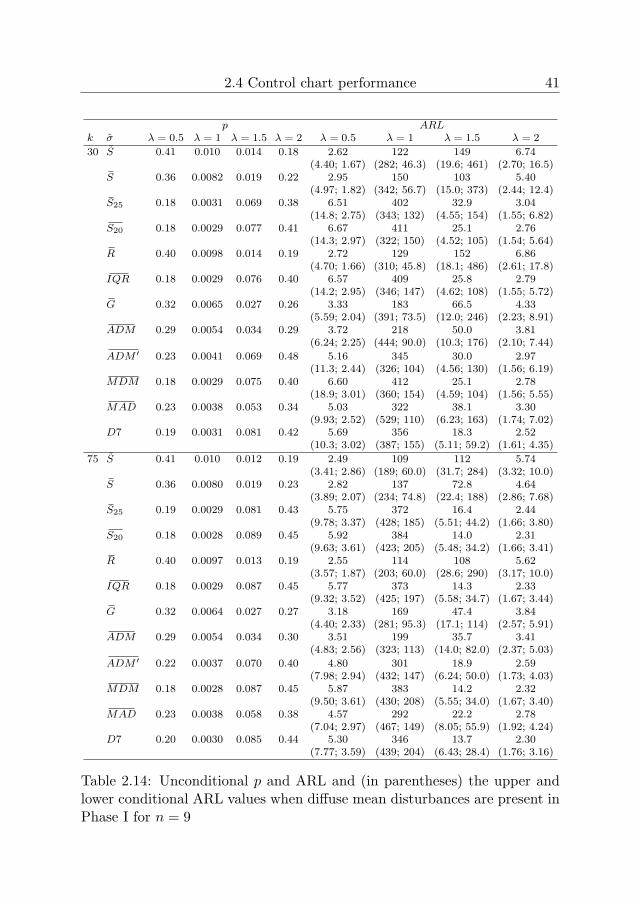
2.4 Control chart performance 41
p ARLk σ λ = 0.5 λ = 1 λ = 1.5 λ = 2 λ = 0.5 λ = 1 λ = 1.5 λ = 2
30 S 0.41 0.010 0.014 0.18 2.62 122 149 6.74(4.40; 1.67) (282; 46.3) (19.6; 461) (2.70; 16.5)
S 0.36 0.0082 0.019 0.22 2.95 150 103 5.40(4.97; 1.82) (342; 56.7) (15.0; 373) (2.44; 12.4)
S25 0.18 0.0031 0.069 0.38 6.51 402 32.9 3.04(14.8; 2.75) (343; 132) (4.55; 154) (1.55; 6.82)
S20 0.18 0.0029 0.077 0.41 6.67 411 25.1 2.76(14.3; 2.97) (322; 150) (4.52; 105) (1.54; 5.64)
R 0.40 0.0098 0.014 0.19 2.72 129 152 6.86(4.70; 1.66) (310; 45.8) (18.1; 486) (2.61; 17.8)
IQR 0.18 0.0029 0.076 0.40 6.57 409 25.8 2.79(14.2; 2.95) (346; 147) (4.62; 108) (1.55; 5.72)
G 0.32 0.0065 0.027 0.26 3.33 183 66.5 4.33(5.59; 2.04) (391; 73.5) (12.0; 246) (2.23; 8.91)
ADM 0.29 0.0054 0.034 0.29 3.72 218 50.0 3.81(6.24; 2.25) (444; 90.0) (10.3; 176) (2.10; 7.44)
ADM ′ 0.23 0.0041 0.069 0.48 5.16 345 30.0 2.97(11.3; 2.44) (326; 104) (4.56; 130) (1.56; 6.19)
MDM 0.18 0.0029 0.075 0.40 6.60 412 25.1 2.78(18.9; 3.01) (360; 154) (4.59; 104) (1.56; 5.55)
MAD 0.23 0.0038 0.053 0.34 5.03 322 38.1 3.30(9.93; 2.52) (529; 110) (6.23; 163) (1.74; 7.02)
D7 0.19 0.0031 0.081 0.42 5.69 356 18.3 2.52(10.3; 3.02) (387; 155) (5.11; 59.2) (1.61; 4.35)
75 S 0.41 0.010 0.012 0.19 2.49 109 112 5.74(3.41; 2.86) (189; 60.0) (31.7; 284) (3.32; 10.0)
S 0.36 0.0080 0.019 0.23 2.82 137 72.8 4.64(3.89; 2.07) (234; 74.8) (22.4; 188) (2.86; 7.68)
S25 0.19 0.0029 0.081 0.43 5.75 372 16.4 2.44(9.78; 3.37) (428; 185) (5.51; 44.2) (1.66; 3.80)
S20 0.18 0.0028 0.089 0.45 5.92 384 14.0 2.31(9.63; 3.61) (423; 205) (5.48; 34.2) (1.66; 3.41)
R 0.40 0.0097 0.013 0.19 2.55 114 108 5.62(3.57; 1.87) (203; 60.0) (28.6; 290) (3.17; 10.0)
IQR 0.18 0.0029 0.087 0.45 5.77 373 14.3 2.33(9.32; 3.52) (425; 197) (5.58; 34.7) (1.67; 3.44)
G 0.32 0.0064 0.027 0.27 3.18 169 47.4 3.84(4.40; 2.33) (281; 95.3) (17.1; 114) (2.57; 5.91)
ADM 0.29 0.0054 0.034 0.30 3.51 199 35.7 3.41(4.83; 2.56) (323; 113) (14.0; 82.0) (2.37; 5.03)
ADM ′ 0.22 0.0037 0.070 0.40 4.80 301 18.9 2.59(7.98; 2.94) (432; 147) (6.24; 50.0) (1.73; 4.03)
MDM 0.18 0.0028 0.087 0.45 5.87 383 14.2 2.32(9.50; 3.61) (430; 208) (5.55; 34.0) (1.67; 3.40)
MAD 0.23 0.0038 0.058 0.38 4.57 292 22.2 2.78(7.04; 2.97) (467; 149) (8.05; 55.9) (1.92; 4.24)
D7 0.20 0.0030 0.085 0.44 5.30 346 13.7 2.30(7.77; 3.59) (439; 204) (6.43; 28.4) (1.76; 3.16)
Table 2.14: Unconditional p and ARL and (in parentheses) the upper andlower conditional ARL values when diffuse mean disturbances are present inPhase I for n = 9

42 Standard Deviation Control Charts
2.5 Real data example
In this section we demonstrate the implementation of the control charts cre-ated above. Our dataset was supplied by Grant and Leavenworth (1988,p.9). The operation concerns thread grinding a fitting for an aircraft hy-draulic system. Table 2.15 shows the pitch diameters of the threads for 20randomly chosen samples. Each sample consists of 5 observations.
The control charting process starts with estimating the in-control stan-dard deviation σ (Phase I). We construct control charts based on the differentPhase I estimators proposed. The estimates derived from these estimatorsare shown in Table 2.16 and are used to determine the Phase II control lim-its. For example, the estimate of σ based on S is equal to 2.972 and Table2.3 shows that the respective factors for the upper and lower control lim-its are 2.352 and 0.171. Consequently the Phase II control limits are 6.990and 0.508. Figure 2.5 compares the Phase II control limits for the proposedestimators.
In the case of ADM ′, we apply a simple subgroup screening method.The factors for the Phase I control limits are 2.089 and 0 for n = 5. Wefirst determine the ADM from the 20 samples, which generates 2.594. ThePhase I control limits are 5.419 and 0. Then we determine the standard de-viation S/c4(5) of each sample and delete samples whose standard deviationfalls outside the initial control limits. For the example discussed here, thestandard deviations of samples 8, 9 and 13 fall outside the control limits.The same procedure is repeated in the second iteration: new values for thein-control σ (2.041) and the Phase I control limits (4.263 and 0) are gener-ated from the remaining samples and any sample whose standard deviationfalls outside the control limits is deleted. In the second iteration, it appearsno longer necessary to delete further samples.
The highest values of UCL and LCL are given by S, while the lowestvalues are given by D7 and ADM ′. Note, however, that the question ofwhich estimator produces the best estimate can not be resolved from such alimited sample.

2.5 Real data example 43
Sample Observations S/c4(5)1 36 35 34 33 32 1.6822 31 31 34 32 30 1.6133 30 30 32 30 32 1.1654 32 33 33 32 35 1.3035 32 34 37 37 35 2.2576 32 32 31 33 33 0.8907 33 33 36 32 31 1.9908 23 33 36 35 36 5.8569 43 36 35 24 31 7.42410 36 35 36 41 41 3.13811 34 38 35 34 38 2.18012 36 38 39 39 40 1.61313 36 40 35 26 33 5.47714 36 35 37 34 33 1.68215 30 37 33 34 35 2.75416 28 31 33 33 33 2.33117 33 30 34 33 35 1.99018 27 28 29 27 30 1.38719 35 36 29 27 32 4.07920 33 35 35 39 36 2.331
Table 2.15: Measurements of pitch diameter of threads on aircraft fittings
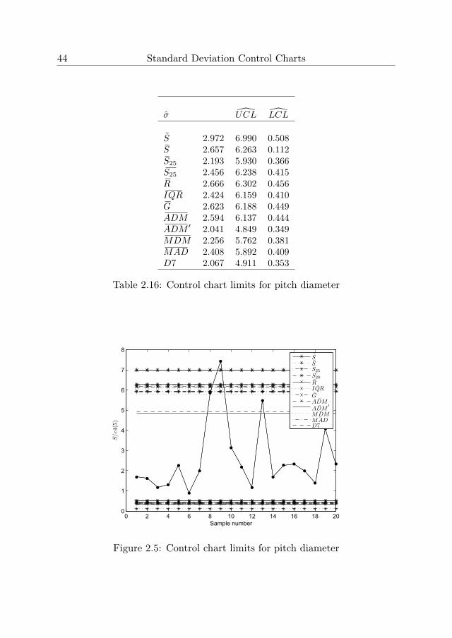
44 Standard Deviation Control Charts
σ UCL LCL
S 2.972 6.990 0.508S 2.657 6.263 0.112S25 2.193 5.930 0.366S25 2.456 6.238 0.415R 2.666 6.302 0.456IQR 2.424 6.159 0.410G 2.623 6.188 0.449ADM 2.594 6.137 0.444ADM ′ 2.041 4.849 0.349MDM 2.256 5.762 0.381MAD 2.408 5.892 0.409D7 2.067 4.911 0.353
Table 2.16: Control chart limits for pitch diameter
0 2 4 6 8 10 12 14 16 18 200
1
2
3
4
5
6
7
8
Sample number
S/c4(5)
S
S
S25
S20
R¯IQR
G¯ADM¯ADM
′
¯MDM¯MAD
D7
Figure 2.5: Control chart limits for pitch diameter

2.6 Concluding remarks 45
2.6 Concluding remarks
In this chapter we have compared 12 different estimators for designing stan-dard deviation control charts and investigated their performance in Phase II.The added value of incorporating a simple screening procedure into an esti-mation method has proven to be substantial. This method performs betterthan estimators which remove samples (S25) or observations (S20 or IQR)beforehand. The disadvantage of removing samples and/or observations be-forehand is that too much information is lost in uncontaminated situationswhile, at the same time, the resulting estimates are biased in contaminatedsituations. The estimator ADM ′ retains far more information, deleting onlyextreme subgroups so that the final estimate is not affected substantially.Moreover, ADM ′ is intuitive and easy to implement. We recommend usingADM ′ when the dataset is likely to be contaminated by localized distur-bances. On the other hand, we prefer D7 when the dataset is likely tobe contaminated by mean diffuse disturbances because D7 is more robustagainst such disturbances. All in all, there appears to be no single bestcontrol-chart method that would cover every process and every company.ASTM 15D (1976, p.143) says it best: “The final justification of a controlchart criterion is its proven ability to detect assignable causes economicallyunder practical conditions.”
2.7 Appendix
The literature proposes several estimators for the standard deviation ofa normal distribution, including estimators based on Gini’s mean differ-ence, Downton’s linear function of order statistics (Downton (1966)) andthe probability-weighted moments estimator (Muhammad et al. (1993)).
Let Xi(1), Xi(2), ..., Xi(n) denote the order statistics of sample i. Accord-ing to David (1968), the sample statistic Gi can also be written as a functionof order statistics
Gi = 2/(n(n− 1))
n∑j=1
(2j − n− 1)Xi(j). (2.16)
Downton (1966) suggested as a possible unbiased estimator of σ the statistic
Di = 1/√π
n∑j=1
(2j − n− 1)Xi(j)/(n(n− 1)), (2.17)

46 Standard Deviation Control Charts
and Muhammad et al. (1993) proposed the so-called probability weightedmoments estimator of σ
Spw,i =√π/n2
n∑j=1
(2j − n− 1)Xi(j). (2.18)
It follows directly from (2.16), (2.17) and (2.18) that
Gi = 2/√πDi = 2n/((n− 1)
√π)Spw,i.

Chapter 3
A Robust Standard DeviationControl Chart
3.1 Introduction
In this chapter we investigate robust Phase I estimators for the subgroupstandard deviation control chart. The estimators considered are the pooledstandard deviation, the robust biweight A estimator of Tatum (1997) andseveral adaptive trimmers. Additionally, we look at an adaptive trimmerbased on the mean deviation from the median, a statistic more resistantto diffuse outliers (see Chapter 2). For diffuse outliers, we think that anindividuals chart would detect outliers more quickly. We therefore include anestimator based on the individuals chart. In order to measure the variabilitywithin and not between subgroups, we correct for differences in the locationbetween subgroups. Moreover, we present an algorithm that combines thelast two approaches. The performance of the estimators is evaluated byassessing their MSE under normality and in the presence of several typesof contaminations. Finally, we derive factors for the Phase II limits of thestandard deviation control chart and assess the performance of the controlcharts by means of a simulation study.
The chapter is structured as follows. The next section introduces thestandard deviation estimators, demonstrates the implementation of the esti-mators by means of a real-world example and assesses their MSE. Next, wepresent the design schemes for the standard deviation control chart and de-rive the Phase II control limits. We then describe the simulation procedure,summarize simulation results and draw some final conclusions.
47

48 A Robust Standard Deviation Control Chart
3.2 Proposed Phase I estimators
In this section we present six Phase I estimators, demonstrate the imple-mentation of the estimators by means of a real data example and assess theefficiency of the estimators in terms of their MSE.
3.2.1 Standard deviation estimators
Recall that Xij , i = 1, 2, ..., k and j = 1, 2, ..., n, denote the Phase I datawith n the subgroup size and k the number of subgroups.
The first estimator of σ is based on the pooled subgroup standard de-viation S (see (2.1)). This estimator provides a basis for comparison undernormality when no contaminations are present. Mahmoud et al. (2010)showed that this estimator is more efficient than the mean of the subgroupstandard deviations and the mean of the subgroup ranges when the data arenormally distributed.
Second, we evaluate a robust estimator proposed by Tatum (1997) (see(2.11)). This estimator is denoted by D7 as in Tatum (1997).
We also include other procedures to obtain σ. The first is a variant ofRocke (1989). Rocke’s procedure first estimates σ by the mean subgrouprange
R =1
k
k∑i=1
Ri,
where Ri is the range of the i-th subgroup. An unbiased estimator of σ undernormality is R/d2(n), where d2(n) is the expected range of a random N(0, 1)subgroup of size n. Values of d2(n) can be found in Duncan (1986), TableM. Any subgroup that exceeds the Phase I control limits is deleted and Ris recomputed from the remaining subgroups. Our approach is similar butcontinues until all subgroup ranges fall between the Phase I control limits.These are set at UCL = UnR/d2(n) and LCL = LnR/d2(n). For simplicity,we derive the factors Un and Ln from the 0.99865 and 0.00135 quantiles ofthe distribution of R/d2(n). Table 3.1 shows the factors for n = 4, 5, 9 aswell as the constants added to obtain unbiased estimates once the data havebeen screened. Note that the factors and the constants are the same fork = 20, 50, 100. The resulting estimator is denoted by Rs.
In addition, we evaluate an adaptive trimmer where the estimate of σ isobtained by the mean subgroup average deviation from the median instead

3.2 Proposed Phase I estimators 49
n = 4 n = 5 n = 9σ Un Ln Constant Un Ln Constant Un Ln Constant
Rs 2.321 0.170 1 2.305 0.172 1 1.950 0.330 1MDs 2.321 0.170 0.998 2.305 0.172 1 1.950 0.330 1
MDi 3 -3 0.990 3 -3 0.975 3 -3 0.986
MDi,s 4.703 0.0018 1 3.225 0.035 1 2.485 0.142 13 -3 0.988 3 -3 0.975 3 -3 0.986
Table 3.1: Factors for Phase I control limits for k = 20, 50, 100
of R. The mean subgroup average deviation from the median is given by
MD =1
k
k∑i=1
MDi,
where MDi is the average absolute deviation from the median Mi of sub-group i defined by,
MDi =n∑
j=1
|Xij −Mi|/n.
An unbiased estimator of σ is MD/t2(n), where t2(n) equals E(MD/σ).Since it is difficult to obtain E(MD) analytically, it is obtained by simula-tion. Extensive tables for t2(n) can be found in Riaz and Saghir (2009). Theadvantage of this estimator is that it is less sensitive to outliers than R (seeChapter 2). The resulting estimator is denoted by MDs. The values usedfor the Phase I control limits and the constants necessary to obtain unbiasedestimates once the data have been screened are given in Table 3.1.
For subgroup control charts, only adaptive trimming methods basedon the subgroup averages or subgroup standard deviations have been pro-posed in the literature so far. For diffuse outliers, however, an individualschart should detect outliers more quickly. We therefore propose a screeningmethod based on an individuals chart. The algorithm first calculates theresiduals by subtracting the subgroup median from each observation in thecorresponding subgroup. This ensures that the variability is measured withinand not between subgroups. Next, an individuals chart of the residuals isconstructed. The location of the chart μ is estimated by the mean of thesubgroup medians, which is zero because the subgroup medians have beensubtracted from the observations, and the standard deviation σ is estimatedby MD. To simplify, the factors for the individuals chart are 3 and -3 (seeTable 3.1). The residuals that fall outside the control limits are excluded

50 A Robust Standard Deviation Control Chart
from the dataset. Then the procedure is repeated: the median values ofthe adjusted subgroups are determined, the residuals are calculated and thecontrol limits of the individuals chart are computed. The residuals that nowexceed the limits are removed. This continues until all residuals fall withinthe control limits. The resulting estimates of σ are slightly biased undernormality. The constants necessary to obtain an unbiased estimate can befound in Table 3.1. The unbiased estimator is denoted by MDi.
The above procedure does not use the spread of the subgroups. There-fore, we finally propose an algorithm that combines the use of an individualschart with subgroup screening. First, an initial estimate of σ is obtainedvia MD. This estimate is then used to construct a standard deviation con-trol chart so that the subgroups can be screened. Adopting R as a chartingstatistic will result in the exclusion of many subgroups, including many un-contaminated observations, when diffuse disturbances are present. For thisreason, we employ IQR for screening purposes. The constants required toobtain an unbiased estimate of σ based on IQR are 0.594 for n = 4, 0.990for n = 5 and 1.144 for n = 9. The values chosen for the Phase I controllimits are presented in Table 3.1. The subgroup screening is continued untilall IQR’s fall within the limits. The resulting estimates of σ are unbiasedand are used to screen observations with an individuals control chart (theprocedure used to derive MDi). The final estimates of σ are slightly biased.The constants necessary to obtain an unbiased estimate can be found inTable 3.1. The unbiased estimator is denoted by MDi,s.
3.2.2 Real data example
In this section we demonstrate the estimation of σ in Phase I. Our datasetwas supplied by Wadsworth et al. (2001, pp. 235-237). The operationconcerns the melt index of a polyethylene compound. The data consist of20 subgroups of size 4 (Table 3.2).
The factors used for the n = 4, k = 20 case are presented in Table 3.1.Note that d2(4) = 2.06, c4(4) = 0.92, t2(4) = 0.66 and dIQR(4) = 0.59.The estimates of σ obtained by S and D7 are determined in one iterationand are 10.14 and 6.59 respectively. The values obtained by Rs and MDs
incorporate subgroup screening. The initial value of Rs is 8.96 and therespective upper and lower control limits are 20.80 and 1.52. The unbiasedestimate of the range (i.e. R/d2(4)) of subgroup 3 falls above the controllimit and so this subgroup is deleted. The second estimate of Rs equals

3.2 Proposed Phase I estimators 51
Sample Observations R/d2(4) S/c4(4) MD/t2(4) IQR/dIQR(4)1 218 224 220 231 6.31 6.23 6.46 6.732 238 236 247 234 6.31 6.23 5.70 3.373 280 228 228 221 28.65 29.70 22.42 04 210 249 241 246 18.94 19.51 16.72 8.425 243 240 230 230 6.31 7.33 8.74 16.846 225 250 258 244 16.03 15.26 14.82 10.107 240 238 240 243 2.43 2.24 1.90 08 244 248 265 234 15.06 14.02 13.30 6.739 238 233 252 243 9.23 8.80 9.12 8.4210 228 238 220 230 8.74 8.03 7.60 3.3711 218 232 230 226 6.80 6.72 6.84 6.7312 226 231 236 242 7.77 7.43 7.98 8.4213 224 221 230 222 4.37 4.38 4.18 3.3714 230 220 227 226 4.86 4.55 4.18 1.6815 224 228 226 240 7.77 7.80 6.84 3.3716 232 240 241 232 4.37 5.35 6.46 13.4717 243 250 248 250 3.40 3.59 3.42 3.3718 247 238 244 230 8.26 8.14 8.74 10.1019 224 228 228 246 10.68 10.69 8.36 020 236 230 230 232 2.91 3.07 3.04 3.37
Table 3.2: Melt index measurements
7.92 and the corresponding Phase I upper and lower control limits are 18.38and 1.35. Now subgroup 4 does not meet the Phase I upper control limitand is removed. The third estimate of Rs is 7.31 and the control limits are16.97 and 1.24. There are no further subgroups whose R/d2(4) exceeds theupper control limit. The resulting unbiased estimate of σ is 7.31. The MDs
procedure works in a similar way. In this case, subgroups 3 and 4 are againdeleted. The final unbiased estimate is 7.03.
For the MDi chart, we use a procedure based on the individuals con-trol chart for the residuals. The residuals are calculated by substracting thesubgroup median from each observation in the corresponding subgroup (seeTable 3.3). The initial value of σ is 8.26 and the control limits of the individ-uals chart are 24.78 and -24.78. One residual in subgroup 3 and one residualin subgroup 4 fall outside the control limits. The corresponding observationsare deleted from the dataset. The subgroup medians are determined from

52 A Robust Standard Deviation Control Chart
Sample Residuals1 -4.0 2.0 -2.0 9.02 1.0 -1.0 10.0 -3.03 52.0 0.0 0.0 -7.04 -33.5 5.5 -2.5 2.55 8.0 5.0 -5.0 -5.06 -22.0 3.0 11.0 -3.07 0.0 -2.0 0.0 3.08 -2.0 2.0 19.0 -12.09 -2.5 -7.5 11.5 2.510 -1.0 9.0 -9.0 1.011 -10.0 4.0 2.0 -2.012 -7.5 -2.5 2.5 8.513 1.0 -2.0 7.0 -1.014 3.5 -6.5 0.5 -0.515 -3.0 1.0 -1.0 13.016 -4.0 4.0 5.0 -4.017 -6.0 1.0 -1.0 1.018 6.0 -3.0 3.0 -11.019 -4.0 0.0 0.0 18.020 5.0 -1.0 -1.0 1.0
Table 3.3: Residuals of melt index measurements
the remaining observations and the residuals are recalculated. The secondestimate of σ is 6.82 and the control limits are now 20.47 and -20.47. Oneresidual in subgroup 6 falls below the lower control limit and so one obser-vation is removed. Again, the medians are determined from the remainingobservations and the residuals are recomputed. The third estimate of σ is6.49 and the control chart has limits at 19.47 and -19.47. There are now noresiduals that fall outside the control limits. The resulting unbiased estimateis 6.55.
For the MDi,s chart, the first part of the procedure screens the subgroupIQR. The respective upper and lower control limits of the IQR chart are38.86 and 0.015. The IQR of subgroups 3, 7 and 19 are 0 and so thesesubgroups are deleted. It is not necessary to delete any further subgroups.Next, individual observations are screened. The estimate of σ is 7.81 andthe upper and lower control limits for the residuals are 23.45 and -23.45.

3.2 Proposed Phase I estimators 53
An outlier in subgroup 4 is deleted. The next estimate of σ is 7.18 withcorresponding control limits 21.55 and -21.55. The outlier in subgroup 6 isremoved from the dataset. Now σ is set at 6.79 with corresponding controllimits 20.37 and -20.37. No further deletions are required. The unbiasedestimate for the MDi,s chart is 6.87.
The final estimates for σ are presented in Table 3.4. The estimate basedon S is higher than the other estimates. This is because S is more sensitiveto outliers than the other estimators.
Chart σ
S 10.14D7 6.59Rs 7.31MDs 7.03
MDi 6.55
MDi,s 6.87
Table 3.4: Final estimates of σ
3.2.3 Efficiency of proposed estimators
In order to evaluate Phase I performance we now assess the MSE of theproposed Phase I estimators. Recall that the MSE is estimated as
MSE =1
N
N∑i=1
(σi − σ)2,
where σi is the value of the unbiased estimate in the i-th simulation run andN is the number of simulation runs. Comparisons are made under normalityand four types of disturbances (cf. Tatum (1997), see Section 2.2.2) but withan error rate of 6% in each case. The number of simulation runs N is equalto 50,000. (Note that Tatum (1997) used 10,000 simulation runs.)
Figure 3.1 shows the MSE values when diffuse symmetric variance dis-turbances are present. The y-intercepts show that the pooled standard de-viation (S) has the lowest MSE when no disturbances are present. However,when the size of the disturbance (a) increases, the MSE increases quickly.The other estimators are more robust against outliers of this type. Those

54 A Robust Standard Deviation Control Chart
that use an individuals control chart to identify individual outliers, i.e. MDi
andMDi,s, coincide and perform best, followed byD7. The estimators basedon only subgroup screening, namely Rs and MDs, turn out to perform lesswell in this situation. The reason is that they screen subgroup dispersion andignore individual outliers. Note that Rs falls far short of MDs, because Rs
uses R (rather than MD) to estimate σ. As R is more sensitive to outliers,the Phase I limits are broader making it more difficult to detect outliers.This effect is particularly significant for n = 9, because a larger subgroup ismore likely to be infected with an outlier.
When asymmetric diffuse disturbances are present (Figure 3.2), the re-sults are comparable to the situation with diffuse symmetric disturbances:MDi and MDi,s coincide and perform best, followed by D7 and MDs. Notethat in this situation S and, for n = 9, R perform badly.
Figure 3.3 shows the results in situations with localized disturbances.The estimators incorporating subgroup screening (Rs and MDs) performbest. The estimator MDi,s performs better than D7 in this situation. Fi-nally, MDi does not perform as well in this case because it does not takeinto account information on the subgroup spread.
The results for diffuse mean disturbance are shown in Figure 3.4. Wecan conclude that S and Rs coincide for n = 9 and perform far worse thanthe other estimators. MDs performs better but not as well as D7 and notas well as the estimators using an individuals chart to identify individualoutliers. The reason is that MDs is less capable of detecting such outliers.The estimators MDi,s and MDi coincide and perform best in this situation.

3.2 Proposed Phase I estimators 55
1 2 3 4 5 60
0.005
0.01
0.015
0.02
0.025
a
MS
E
SD7
Rs
MDs
MDi
MDi,s
(a)
1 2 3 4 5 60
0.002
0.004
0.006
0.008
0.01
0.012
0.014
0.016
0.018
0.02
a
MS
E
SD7
Rs
MDs
MDi
MDi,s
(b)
1 2 3 4 5 60
0.005
0.01
0.015
0.02
0.025
0.03
0.035
a
MS
E
SD7
Rs
MDs
MDi
MDi,s
(c)
1 2 3 4 5 60
0.005
0.01
0.015
0.02
0.025
a
MS
E
SD7
Rs
MDs
MDi
MDi,s
(d)
Figure 3.1: MSE of estimators when symmetric diffuse variance disturbancesare present. (a) n = 5, k = 50 (b) n = 5, k = 100 (c) n = 9, k = 50 (d)n = 9, k = 100

56 A Robust Standard Deviation Control Chart
0 1 2 3 4 50
0.005
0.01
0.015
0.02
0.025
Multiplier
MS
E
SD7
Rs
MDs
MDi
MDi,s
(a)
0 1 2 3 4 50
0.005
0.01
0.015
b
MS
E
SD7
Rs
MDs
MDi
MDi,s
(b)
0 1 2 3 4 50
0.002
0.004
0.006
0.008
0.01
0.012
0.014
0.016
0.018
0.02
Multiplier
MS
E
SD7
Rs
MDs
MDi
MDi,s
(c)
0 1 2 3 4 50
0.001
0.002
0.003
0.004
0.005
0.006
0.007
0.008
0.009
0.01
Multiplier
MS
E
SD7
Rs
MDs
MDi
MDi,s
(d)
Figure 3.2: MSE of estimators when asymmetric diffuse variance distur-bances are present. (a) n = 5, k = 50 (b) n = 5, k = 100 (c) n = 9, k = 50(d) n = 9, k = 100
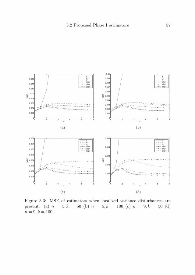
3.2 Proposed Phase I estimators 57
1 2 3 4 5 60
0.002
0.004
0.006
0.008
0.01
0.012
0.014
0.016
a
MS
E
SD7
Rs
MDs
MDi
MDi,s
(a)
1 2 3 4 5 60
0.001
0.002
0.003
0.004
0.005
0.006
0.007
0.008
0.009
0.01
a
MS
E
SD7
Rs
MDs
MDi
MDi,s
(b)
1 2 3 4 5 60
0.001
0.002
0.003
0.004
0.005
0.006
0.007
0.008
a
MS
E
SD7
Rs
MDs
MDi
MDi,s
(c)
1 2 3 4 5 60
0.001
0.002
0.003
0.004
0.005
a
MS
E
SD7
Rs
MDs
MDi
MDi,s
(d)
Figure 3.3: MSE of estimators when localized variance disturbances arepresent. (a) n = 5, k = 50 (b) n = 5, k = 100 (c) n = 9, k = 50 (d)n = 9, k = 100

58 A Robust Standard Deviation Control Chart
0 2 4 6 8 100
0.02
0.04
0.06
0.08
0.1
0.12
0.14
0.16
0.18
0.2
b
MS
E
SD7
Rs
MDs
MDi
MDi,s
(a)
0 2 4 6 8 100
0.01
0.02
0.03
0.04
0.05
0.06
0.07
0.08
0.09
0.1
b
MS
E
SD7
Rs
MDs
MDi
MDi,s
(b)
0 2 4 6 8 100
0.01
0.02
0.03
0.04
0.05
0.06
0.07
0.08
b
MS
E
SD7
Rs
MDs
MDi
MDi,s
(c)
0 2 4 6 8 100
0.01
0.02
0.03
0.04
0.05
0.06
0.07
0.08
b
MS
E
SD7
Rs
MDs
MDi
MDi,s
(d)
Figure 3.4: MSE of estimators when diffuse mean disturbances are present.(a) n = 5, k = 50 (b) n = 5, k = 100 (c) n = 9, k = 50 (d) n = 9, k = 100

3.3 Derivation of Phase II control limits 59
3.3 Derivation of Phase II control limits
Equation (1.3) gives control limits for the standard deviation control chartwith σ estimated in Phase I. We estimate λσ in Phase II by S/c4(n) for allcharts. One of the criteria used to assess Phase II performance is the ARL.To allow comparison, Un and Ln are chosen such that the unconditional ARLequals 370 and, for each chart, the ARL’s for the upper and lower controllimits are similar. Un and Ln can not be obtained easily in analytic formand are obtained from 50,000 simulation runs. Table 3.5 presents Un andLn for n = 5, 9 and k = 50, 100.
k = 50 k = 100n σ Un Ln Un Ln
5 S 2.230 0.163 2.236 0.169D7 2.225 0.162 2.236 0.167Rs 2.226 0.163 2.236 0.168MDs 2.226 0.162 2.237 0.167
MDi 2.217 0.160 2.333 0.166
MDi,s 2.217 0.160 2.333 0.166
9 S 1.832 0.343 1.835 0.347D7 1.830 0.341 1.834 0.346Rs 1.831 0.342 1.835 0.347MDs 1.830 0.342 1.835 0.346
MDi 1.829 0.341 1.833 0.346
MDi,s 1.829 0.341 1.833 0.346
Table 3.5: Factors Un and Ln to determine Phase II control limits for n = 5, 9and k = 50, 100
3.4 Control chart performance
We now evaluate the effect of the proposed estimators on the Phase II perfor-mance of the standard deviation control chart. We consider the same PhaseI estimators as those used to asses the MSE with a, b and the multiplierequal to 4 to simulate the contaminated cases (see Section 2.2.2).
The performance of the control charts is assessed in terms of the uncon-ditional ARL and SDRL. We compute these run length characteristics in anin-control and several out-of-control situations. We consider different shifts

60 A Robust Standard Deviation Control Chart
in the standard deviation λσ, setting λ equal to 0.6, 1, 1.2 and 1.4. Theperformance characteristics are obtained by simulation. The next two sec-tions describe the simulation method and the results for the control chartsconstructed in the uncontaminated and contaminated situations.
3.4.1 Simulation procedure
We use the same procedure as in Section 2.4.1. Enough replications of theprocedure were performed to obtain sufficiently small relative estimated stan-dard errors for the ARL. The relative standard error never exceeds 0.76%.
3.4.2 Simulation results
The ARL and SDRL are obtained in the in-control situation and in the out-of-control situation. When the process is in control, i.e. when λ = 1, wewant the ARL and SDRL to be close to their intended values, namely 370.In the out-of-control situation, i.e. when λ �= 1, we want to detect changesin the standard deviation as soon as possible, so the ARL should be as lowas possible.
Table 3.6 shows the ARL and SDRL for the situation when the Phase Idata are uncontaminated and normally distributed. The ARL is very similaracross charts and the SDRL is slightly higher for the MDi and MDi,s charts.
Tables 3.7 and 3.8 show that, when there are disturbances in the Phase Idata, the ARL values increase considerably. Thus, when the Phase I data arecontaminated, changes in the process standard deviation are less likely to bedetected. With diffuse disturbances (Table 3.7 and second half of Table 3.8),their impact is smallest for the charts based on MDi, MDi,s and D7. Whenthere are localized disturbances (second half of Table 3.8), the charts basedon Rs, MDs and MDi,s perform best, because these charts trim extremesubgroups. Note that in a number of cases the S, Rs and MDs charts areARL-biased: the in-control ARL is lower than the out-of-control ARL (cf.Jensen et al. (2006)).
Overall, the MDi,s chart performs best. Under normality, this chartalmost matches the standard chart based on S and, in the presence of anycontamination, the chart outperforms the alternatives.
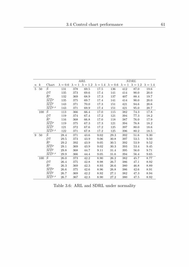
3.4 Control chart performance 61
ARL SDRLn k Chart λ = 0.6 λ = 1 λ = 1.2 λ = 1.4 λ = 0.6 λ = 1 λ = 1.2 λ = 1.4
5 50 S 131 378 69.5 17.5 136 412 87.0 19.6D7 135 373 69.6 17.4 141 414 90.0 20.0Rs 132 369 68.9 17.3 137 407 88.4 19.7MDs 135 375 69.7 17.4 141 414 90.0 20.0MDi 143 371 70.0 17.3 151 421 94.6 20.6MDi,s 143 371 69.9 17.4 151 421 95.0 20.7
100 S 113 366 66.4 17.0 115 382 74.3 17.8D7 119 374 67.4 17.2 121 394 77.3 18.2Rs 116 368 66.8 17.0 118 387 76.0 17.9MDs 119 375 67.3 17.3 121 394 76.8 18.2MDi 121 372 67.6 17.2 125 397 80.0 18.6MDi,s 122 371 67.8 17.2 125 396 80.2 18.5
9 50 S 28.4 371 43.6 9.02 29.3 392 51.6 9.30D7 29.5 373 43.9 9.06 30.8 397 53.5 9.50Rs 29.2 392 43.9 9.05 30.5 392 53.9 9.52MDs 29.1 369 43.9 9.02 30.3 393 53.4 9.45MDi 29.8 368 44.7 9.11 31.4 395 56.0 9.71MDi,s 29.9 366 44.4 9.05 31.6 394 56.4 9.65
100 S 26.0 373 42.2 8.90 26.2 382 45.7 8.77D7 26.4 375 42.8 8.98 26.7 386 47.1 8.92Rs 26.3 369 42.3 8.93 26.6 380 46.8 8.89MDs 26.6 375 42.6 8.96 26.8 386 42.6 8.91MDi 26.7 369 42.2 8.92 27.1 382 47.3 8.94MDi,s 26.7 367 42.3 8.90 27.2 380 47.5 8.92
Table 3.6: ARL and SDRL under normality

62 A Robust Standard Deviation Control Chart
ARL SDRLn k Chart λ = 0.6 λ = 1 λ = 1.2 λ = 1.4 λ = 0.6 λ = 1 λ = 1.2 λ = 1.4
N(0, 1) 5 50 S 43.9 297 425 303 50.8 337 452 391& D7 102 484 159 34.7 108 498 215 47.2N(0, 4) Rs 92.2 464 206 50.1 99.9 479 286 87.2(sym.) MDs 101 474 171 38.2 108 492 171 58.6
MDi 123 443 114 25.3 131 479 164 34.2MDi,s 122 446 114 25.6 131 481 164 34.6
100 S 35.9 248 413 308 38.5 269 425 362D7 89.7 476 152 32.8 91.4 479 182 37.8Rs 81.4 458 191 42.0 84.6 462 239 55.2MDs 89.0 470 159 34.4 89.0 470 159 42.0MDi 104 443 107 24.3 108 458 133 28.0MDi,s 104 444 108 28.0 108 458 134 28.0
9 50 S 5.47 114 317 286 5.92 148 354 351D7 19.9 433 109 17.0 20.8 440 144 20.1Rs 14.3 336 238 47.5 368 238 47.5MDs 18.9 410 128 19.6 20.3 421 178 26.3MDi 23.8 420 75.2 12.9 25.3 433 102 15.0MDi,s 23.7 421 75.9 13.0 25.2 434 103 15.0
100 S 4.86 95.6 305 302 4.75 110 331 345D7 17.9 420 104 16.5 18.0 423 122 17.6Rs 12.9 323 225 36.0 12.9 343 276 53.4MDs 17.3 409 118 18.2 17.3 414 118 18.2MDi 21.3 420 70.0 12.4 21.7 424 82.2 13.1MDi,s 21.2 420 70.6 12.5 21.6 424 83.2 13.2
N(0, 1) 5 50 S 23.2 149 231 266 38.4 243 325 355& D7 112 461 121 26.9 118 483 164 34.2N(0, 4) Rs 108 450 133 29.9 115 472 191 43.6(asym.) MDs 115 449 119 26.6 121 475 168 35.7
MDi 130 419 92.7 21.7 138 461 131 27.5MDi,s 130 422 95.0 21.9 138 463 135 27.9
100 S 14.9 98.0 183 262 21.3 147 253 262D7 98.0 458 116 25.9 100 466 138 28.8Rs 95.2 447 122 27.3 97.9 455 151 31.9MDs 101 448 111 25.1 103 458 111 28.5MDi 111 419 88.9 21.1 114 438 109 23.5MDi,s 110 421 89.8 21.2 114 440 109 23.7
9 50 S 2.34 33.3 93.6 165 3.27 79.5 186 263D7 22.7 435 80.0 13.5 23.7 443 104 15.2Rs 18.8 399 140 22.6 20.6 415 207 39.7MDs 22.5 418 83.3 14.0 23.9 429 116 16.7MDi 26.0 407 61.1 11.2 27.5 425 80.5 12.6MDi,s 25.7 409 61.7 11.3 27.3 426 81.4 12.7
100 S 1.79 18.8 59.5 140 1.72 34.5 112 220D7 20.4 429 75.9 13.2 20.5 431 87.2 13.7Rs 17.1 396 123 18.9 17.6 403 159 22.9MDs 20.6 424 77.4 13.4 20.6 428 92.7 14.3MDi 23.2 408 57.4 10.9 23.6 415 66.3 11.2MDi,s 23.1 411 67.4 11.4 23.4 417 67.4 11.4
Table 3.7: ARL and SDRL when contaminations are present in Phase I

3.4 Control chart performance 63
ARL SDRLn k Chart λ = 0.6 λ = 1 λ = 1.2 λ = 1.4 λ = 0.6 λ = 1 λ = 1.2 λ = 1.4
N(0, 1) 5 50 S 42.8 293 436 308 48.3 330 459 390& D7 118 442 103 23.5 124 469 139 28.7N(0, 4) Rs 129 384 77.1 18.7 134 422 103 22.2(loc.) MDs 131 391 78.5 19.0 137 431 106 22.9
MDi 127 428 100 22.9 136 468 143 29.5MDi,s 135 404 85.9 20.4 144 451 122 25.7
100 S 35.6 245 419 312 37.7 263 429 361D7 103 441 99.1 23.0 105 451 117 25.1Rs 113 382 73.1 18.3 113 401 85.1 19.7MDs 115 392 74.6 18.5 117 411 87.9 20.0MDi 109 429 95.0 22.1 112 446 117 25.0MDi,s 115 403 81.6 19.7 118 425 99.6 21.9
9 50 S 5.34 110 324 295 5.55 136 357 254D7 24.3 427 67.9 12.1 25.4 438 86.9 13.3Rs 28.8 372 46.0 9.31 30.2 396 57.8 9.93MDs 28.6 372 46.0 9.31 30.0 396 57.5 9.91MDi 23.9 420 74.4 12.8 25.5 433 100 14.7MDi,s 28.9 377 49.1 9.68 30.7 404 64.4 10.6
100 S 4.80 93.8 306 309 4.59 105 329 347D7 21.8 425 65.3 11.9 22.0 428 74.0 12.2Rs 25.9 372 43.9 9.12 26.2 384 49.1 9.14MDs 26.2 380 44.1 9.19 26.5 391 49.0 9.20MDi 21.4 420 69.4 12.4 21.8 424 81.6 13.0MDi,s 25.8 379 46.1 9.42 26.3 391 52.8 9.59
N(0, 1) 5 50 S 40.2 280 470 335 42.8 300 480 395& D7 80.3 471 286 72.8 86.7 483 359 117N(4, 1) Rs 54.1 358 431 207 61.1 384 466 292
MDs 65.0 409 394 144 73.0 431 450 220MDi 115 447 152 64.4 127 481 237 64.4MDi,s 115 449 152 63.5 127 483 234 63.5
100 S 34.4 237 434 328 35.1 246 439 360D7 70.0 448 282 65.2 72.5 454 327 85.4Rs 46.6 320 436 193 49.2 336 450 248MDs 55.9 378 399 129 58.9 392 429 173MDi 98.3 451 136 30.2 103 464 183 39.7MDi,s 98.0 451 136 30.2 103 464 182 39.4
9 50 S 5.04 101 325 321 4.87 114 348 363D7 14.4 358 230 35.1 15.3 380 291 51.4Rs 5.59 117 341 292 5.84 144 367 353MDs 9.53 231 370 99.0 10.4 266 404 151MDi 22.8 409 93.6 15.2 25.0 425 142 20.9MDi,s 22.8 410 92.1 15.2 25.0 425 140 21.0
100 S 4.67 89.6 302 327 4.29 94.8 316 351D7 12.9 330 225 32.2 13.0 343 262 38.7Rs 5.00 99.7 322 294 4.77 110 338 332MDs 8.59 207 387 88.6 8.64 226 403 117MDi 20.4 413 82.2 13.9 21.0 418 105 15.6MDi,s 20.4 414 81.7 13.8 21.0 418 104 15.4
Table 3.8: ARL and SDRL when contaminations are present in Phase I

64 A Robust Standard Deviation Control Chart
3.5 Concluding remarks
In this chapter we consider several estimators of the standard deviation inPhase I of the control charting process. We have found that the perfor-mance of certain robust estimators is almost identical to the pooled sub-group standard deviation under normality, while the benefit of using suchrobust estimators can be substantial when there are disturbances. FollowingRocke (1989, 1992), we have considered estimators that include a procedurefor subgroup screening, but whereas Rocke used R, we have used the aver-age deviation from the median. This estimator performs better when thereare localized disturbances and is much more robust against diffuse variancedisturbances. However, when there are diffuse mean disturbances, the pro-cedure loses efficiency.
To address this problem, we have proposed other algorithms, based on aprocedure that also screens for individual outliers. The algorithms removethe variation between subgroups, so that only the variation within subgroupsis measured. We have shown that these algorithms are very effective whenthere are diffuse disturbances. When there might also be localized distur-bances, the method can be combined with subgroup screening based on theIQR. The latter procedure reveals a performance very similar to the ro-bust estimator for the standard deviation control chart proposed by Tatum(1997). We think that this is a noteworthy outcome since the procedureis simple and intuitive. Moreover, it can be used to estimate σ in otherpractical applications.

Chapter 4
Location Estimators for X ControlCharts
4.1 Introduction
This chapter studies estimation methods for the location parameter. We con-sider several robust location estimators as well as several estimation methodsbased on a Phase I analysis (recall that this is the use of a control chart tostudy a historical dataset retrospectively to identify disturbances). In addi-tion, we propose a new type of Phase I analysis. The estimation methodsare evaluated in terms of their MSE and their effect on the X control chartsused for real-time process monitoring (Phase II). It turns out that the PhaseI control chart based on the trimmed trimean far outperforms the existingestimation methods. This method has therefore proven to be very suitablefor determining X Phase II control chart limits.
The remainder of the chapter is organized as follows. First, we presentseveral Phase I sample statistics for the process location and compare theirMSE. Then we describe some existing Phase I control charts and presenta new algorithm for Phase I analysis. Following that, we present the de-sign schemes for the X Phase II control chart and derive the control limits.Next, we describe the simulation procedure and present the effect of theproposed methods on Phase II performance. The final section offers somerecommendations.
65
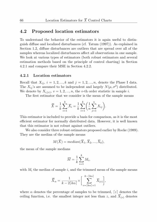
66 Location Estimators for X Control Charts
4.2 Proposed location estimators
To understand the behavior of the estimators it is again useful to distin-guish diffuse and localized disturbances (cf. Tatum (1997)). As explained inSection 1.2, diffuse disturbances are outliers that are spread over all of thesamples whereas localized disturbances affect all observations in one sample.We look at various types of estimators (both robust estimators and severalestimation methods based on the principle of control charting) in Section4.2.1 and compare their MSE in Section 4.2.2.
4.2.1 Location estimators
Recall that Xij , i = 1, 2, ..., k and j = 1, 2, ..., n, denote the Phase I data.The Xij ’s are assumed to be independent and largely N(μ, σ2) distributed.We denote by Xi,(v), v = 1, 2, ..., n, the v-th order statistic in sample i.
The first estimator that we consider is the mean of the sample means
X =1
k
k∑i=1
Xi =1
k
k∑i=1
(1
n
n∑j=1
Xij
).
This estimator is included to provide a basis for comparison, as it is the mostefficient estimator for normally distributed data. However, it is well knownthat this estimator is not robust against outliers.
We also consider three robust estimators proposed earlier by Rocke (1989).They are the median of the sample means
M(X) = median(X1, X2, ..., Xk),
the mean of the sample medians
M =1
k
k∑i=1
Mi,
with Mi the median of sample i, and the trimmed mean of the sample means
Xα =1
k − 2�kα�×[ k−�kα�∑v=�kα�+1
X(v)
],
where α denotes the percentage of samples to be trimmed, �z� denotes theceiling function, i.e. the smallest integer not less than z, and X(v) denotes

4.2 Proposed location estimators 67
the v-th ordered value of the sample means. In our study, we consider the20% trimmed mean, which trims the six smallest and the six largest samplemeans when k = 30. Of course other trimming percentages could have beenused. In fact, we have also used 10% and 25% but the results with 20% arerepresentative for this estimator.
Furthermore, our analysis includes the Hodges-Lehmann estimator (Hod-ges and Lehmann (1963)), an estimator based on the so-called Walsh aver-ages. The h (= n(n+ 1)/2) Walsh averages of sample i are
Wi,k,l = (Xi,k +Xi,l)/2, k = 1, 2, ..., n, l = 1, 2, ..., n, k ≤ l.
The Hodges-Lehmann estimate for sample i, denoted by HLi, is defined asthe median of the Walsh averages. Alloway and Raghavachari (1991) con-ducted a Monte Carlo simulation to determine whether the mean or the me-dian of the sample Hodges-Lehmann estimates should be used to determinethe final location estimate. They concluded that the mean of the samplevalues should be used
HL =1
k
k∑i=1
HLi
and that the resulting estimate is unbiased.
We also include the trimean statistic. The trimean of sample i is theweighted average of the sample median and the two other quartiles
TMi = (Qi,1 + 2Qi,2 +Qi,3)/4,
where Qi,q is the q-th quartile of sample i, q = 1, 2, 3 (cf. Tukey (1997)and Wang et al. (2007)). It also equals the average of the median and the
midhinge 1/2
(Qi,2+
Qi,1+Qi,3
2
)(cf. Weisberg (1992)). We use the following
definitions for the quartiles: Qi,1 = Xi,(a) and Qi,3 = Xi,(b) with a = �n/4�and b = n− a+ 1. This means that Qi,1 and Qi,3 are defined as the secondsmallest and the second largest observations respectively for 5 ≤ n ≤ 8,and as the third smallest and the third largest values respectively for 9 ≤n ≤ 12. Like the median and the midhinge, but unlike the sample mean,the trimean is a statistically resistant L-estimator (a linear combination oforder statistics), with a breakdown point of 25% (see Wang et al. (2007)).According to Tukey (1977), using the trimean instead of the median givesa more useful assessment of location or centering. According to Weisberg

68 Location Estimators for X Control Charts
(1992), the “statistical resistance” benefit of the trimean as a measure of thecenter of a distribution is that it combines the median’s emphasis on centervalues with the midhinge’s attention to the extremes. The trimean is almostas resistant to extreme scores as the median and is less subject to samplingfluctuations than the arithmetic mean in extremely skewed distributions.Asymptotic distributional results of the trimean can be found in Wang etal. (2007). The location estimate analyzed below is the mean of the sampletrimeans, i.e.
TM =1
k
k∑i=1
TMi.
Finally, we consider a statistic that is expected to be robust against bothdiffuse and localized disturbances, namely the trimmed mean of the sampletrimeans, defined by
TMα =1
k − 2�kα�×[ k−�kα�∑v=�kα�+1
TM(v)
],
where TM(v) denotes the v-th ordered value of the sample trimeans. Weconsider the 20% trimmed trimean, which trims the six smallest and the sixlargest sample trimeans when k = 30.
The estimators outlined above are summarized in Table 4.1.
Estimator Notation
Mean of sample means XMedian of sample means M(X)Mean of sample medians M
20% trimmed mean of sample means X20
Mean of sample Hodges-Lehmann HLMean of sample trimeans TM20% trimmed mean of sample trimeans TM20
Table 4.1: Proposed location estimators

4.2 Proposed location estimators 69
4.2.2 Efficiency of proposed estimators
As in Chapters 2 and 3, we follow Tatum (1997) and evaluate the estimatorsin terms of their MSE. In this case, the MSE is estimated as
MSE =1
N
N∑i=1
(μi − μ
σ
)2
.
We include the uncontaminated case, i.e. the situation where all the Xij ’sare from the N(0, 1) distribution, as well as five types of disturbances. Theyare the four models described in Section 2.2.2 and
5. A model for localized mean disturbances in which observations in3 out of 30 samples are drawn from the N(a, 1) distribution, with a =0.5, 1.0, ..., 5.5, 6.0.
1 2 3 4 5 60.006
0.008
0.01
0.012
0.014
0.016
0.018
0.02
a
MS
E
¯X
M (X)
M¯X20
HL¯TM¯TM 20
(a)
1 2 3 4 5 60.003
0.004
0.005
0.006
0.007
0.008
0.009
0.01
0.011
a
MS
E
¯X
M (X)
M¯X20
HL¯TM¯TM 20
(b)
Figure 4.1: MSE of estimators when symmetric diffuse variance disturbancesare present for k = 30 (a) n = 5 (b) n = 9

70 Location Estimators for X Control Charts
0 1 2 3 4 50.006
0.008
0.01
0.012
0.014
0.016
0.018
0.02
0.022
0.024
Multiplier
MS
E
¯X
M (X)
M¯X20
HL¯TM¯TM 20
(a)
0 1 2 3 4 5
0.004
0.006
0.008
0.01
0.012
0.014
MultiplierM
SE
¯X
M (X)
M¯X20
HL¯TM¯TM 20
(b)
Figure 4.2: MSE of estimators when asymmetric diffuse variance distur-bances are present for k = 30 (a) n = 5 (b) n = 9
1 2 3 4 5 60.005
0.01
0.015
0.02
0.025
0.03
0.035
0.04
0.045
a
MS
E
¯X
M (X)
M¯X20
HL¯TM¯TM 20
(a)
1 2 3 4 5 6
0.004
0.006
0.008
0.01
0.012
0.014
0.016
0.018
0.02
0.022
0.024
a
MS
E
¯X
M (X)
M¯X20
HL¯TM¯TM 20
(b)
Figure 4.3: MSE of estimators when localized variance disturbances arepresent for k = 30 (a) n = 5 (b) n = 9

4.2 Proposed location estimators 71
0 2 4 6 8 100.005
0.01
0.015
0.02
0.025
0.03
0.035
0.04
0.045
0.05
MS
E
b
¯X
M (X)
M¯X20
HL¯TM¯TM 20
(a)
0 2 4 6 8 10
0.004
0.006
0.008
0.01
0.012
0.014
0.016
0.018
0.02
0.022
0.024
b
MS
E
¯X
M (X)
M¯X20
HL¯TM¯TM 20
(b)
Figure 4.4: MSE of estimators when diffuse mean disturbances are presentfor k = 30 (a) n = 5 (b) n = 9
0 1 2 3 4 5 60.005
0.01
0.015
0.02
0.025
b
MS
E
¯X
M (X)
M¯X20
HL¯TM¯TM 20
(a)
0 1 2 3 4 5 60.003
0.004
0.005
0.006
0.007
0.008
0.009
0.01
0.011
0.012
0.013
b
MS
E
¯X
M (X)
M¯X20
HL¯TM¯TM 20
(b)
Figure 4.5: MSE of estimators when localized mean disturbances are presentfor k = 30 (a) n = 5 (b) n = 9

72 Location Estimators for X Control Charts
The figures show that in the uncontaminated situation the most efficientestimator is X as was to be expected. The estimators HL, X20 and TMare slightly less efficient followed by TM20, M and M(X), the reason beingthat they use less information.
When diffuse symmetric variance disturbances are present (Figure 4.1),the best performing estimators are HL and TM . The reason why TMperforms well in this situation is that it filters out the extreme high and lowvalues in each sample. HL also performs well because it obtains the samplestatistic using the median of the Walsh averages, which is not sensitive tooutliers. M and TM20 are as efficient in the contaminated situation asin the uncontaminated situation but they are outperformed by HL andTM because the latter estimators use more information. It is worth notingthat the traditional estimator X shows relatively bad results despite thesymmetric character of the outliers. M(X) andX20 do not perform very wellbecause these estimators focus on extreme samples whereas in the presentsituation the outliers are spread over all of the samples so that the non-trimmed samples are also infected.
When asymmetric variance disturbances are present (Figure 4.2), themost efficient estimators are TM , TM20, HL and M , performing partic-ularly well relative to the other estimators for larger sample sizes. As forthe symmetric diffuse case, the estimators that include a method to trimobservations within a sample perform better than the methods that focuson sample trimming.
In the case of localized variance disturbances (Figure 4.3), the estimatorsbased on the principle of trimming sample means rather than within-sampleobservations - X20, TM20 andM(X) - have the lowest MSE . The estimators
X, HL, TM and in particular M are less successful because these statisticsonly perform well if no more than a few observations in a sample are infectedrather than all observations, as is the case here.
When diffuse mean disturbances are present (Figure 4.4), the results arecomparable to the situation where there are diffuse asymmetric variancedisturbances: M , TM20 and TM perform best, followed by HL. Note thatin this situation X, M(X) and X20 perform badly.
When localized mean disturbances are present (Figure 4.5), the resultsare comparable to the situation where there are localized variance distur-bances: the estimators based on the principle of trimming sample means,namely X20, M(X) and TM20, perform best.
To summarize, M , TM and TM20 have the lowest MSE when there are

4.3 Proposed control chart location estimators 73
diffuse disturbances. M and TM lose their efficiency advantage when con-taminations take the form of localized mean or variance disturbances. Insuch situations, M(X), X20 and TM20, which involve trimming the sam-ple means, perform relatively well. TM20 has the best performance overallbecause it is reasonably robust against all types of contaminations.
4.3 Proposed control chart location estimators
In-control process parameters can be obtained not only via robust statisticsbut also via Phase I control charting. In the latter case, control charts areused retrospectively to study a historical dataset and identify samples thatare deemed out of control. The process parameters are then estimated fromthe in-control samples. In this section, we consider several Phase I analyseswhich apply the principle of control charting in order to generate robustestimates of process location. We study a Phase I control chart based on thecommonly used estimator X and a Phase I control chart based on the meanrank proposed by Jones-Farmer et al. (2009). Moreover, we propose twonew types of Phase I analyses. The next section presents the various PhaseI control charts and the following section shows the MSE of the proposedestimation methods.
4.3.1 Phase I control charts
The standard procedure in practice is to use the estimator X for construct-ing the X Phase I control chart limits. The respective upper and lowercontrol limits of the Phase I chart are given by UCL ¯X = X + 3σ/
√n and
LCL ¯X = X − 3σ/√n, where we estimate σ by the robust standard devia-
tion estimator proposed by Tatum (1997), using the corrected normalizing
constants presented in Chapter 2. The samples whose Xi fall above UCL ¯X
or below LCL ¯X are eliminated from the Phase I dataset. The final locationestimate is the mean of the sample means of the remaining samples
X′=
1
k′∑iεK
Xi × ILCL ¯X
≤Xi≤UCL ¯X
(Xi),
with K the set of samples which are not excluded, k′ the number of non-excluded samples and I the indicator function. This adaptive trimmed meanestimator is denoted by ATM ¯X .
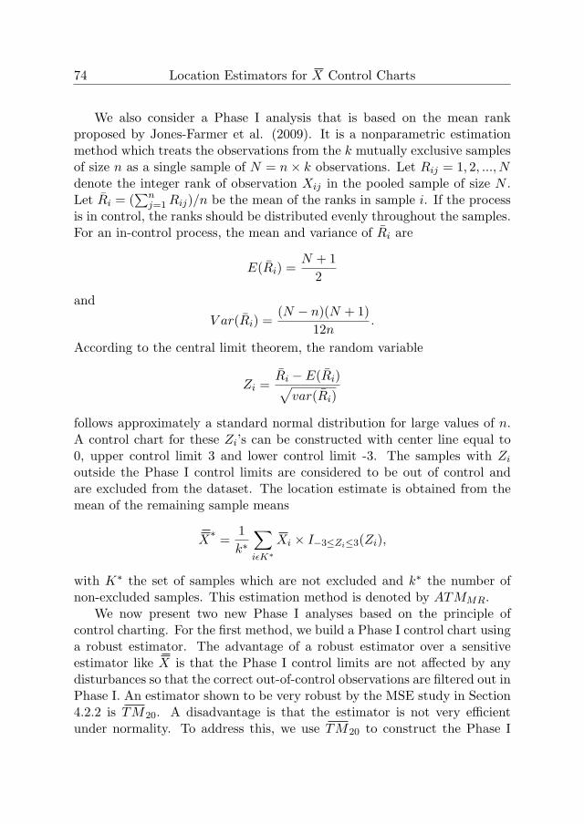
74 Location Estimators for X Control Charts
We also consider a Phase I analysis that is based on the mean rankproposed by Jones-Farmer et al. (2009). It is a nonparametric estimationmethod which treats the observations from the k mutually exclusive samplesof size n as a single sample of N = n× k observations. Let Rij = 1, 2, ..., Ndenote the integer rank of observation Xij in the pooled sample of size N .Let Ri = (
∑nj=1Rij)/n be the mean of the ranks in sample i. If the process
is in control, the ranks should be distributed evenly throughout the samples.For an in-control process, the mean and variance of Ri are
E(Ri) =N + 1
2
and
V ar(Ri) =(N − n)(N + 1)
12n.
According to the central limit theorem, the random variable
Zi =Ri − E(Ri)√
var(Ri)
follows approximately a standard normal distribution for large values of n.A control chart for these Zi’s can be constructed with center line equal to0, upper control limit 3 and lower control limit -3. The samples with Zi
outside the Phase I control limits are considered to be out of control andare excluded from the dataset. The location estimate is obtained from themean of the remaining sample means
X∗=
1
k∗∑iεK∗
Xi × I−3≤Zi≤3(Zi),
with K∗ the set of samples which are not excluded and k∗ the number ofnon-excluded samples. This estimation method is denoted by ATMMR.
We now present two new Phase I analyses based on the principle ofcontrol charting. For the first method, we build a Phase I control chart usinga robust estimator. The advantage of a robust estimator over a sensitiveestimator like X is that the Phase I control limits are not affected by anydisturbances so that the correct out-of-control observations are filtered out inPhase I. An estimator shown to be very robust by the MSE study in Section4.2.2 is TM20. A disadvantage is that the estimator is not very efficientunder normality. To address this, we use TM20 to construct the Phase I

4.3 Proposed control chart location estimators 75
limits with which we screen Xi for disturbances, but then use the efficientestimator X to obtain the location estimate from the remaining samples.The Phase I control limits are given by UCL ¯TM20
= TM20 + 3σ/√n and
LCL ¯TM20= TM20 − 3σ/
√n, where we estimate σ by Tatum’s estimator.
We then plot the Xi’s on the Phase I control chart. The samples whose Xi
falls outside the limits are regarded as out of control and removed from thedataset. The remaining samples are used to determine the grand samplemean
X#=
1
k#
∑iεK#
Xi × ILCL ¯TM20
≤Xi≤UCL ¯TM20
(Xi),
with K# the set of samples which are not excluded and k# the number ofnon-excluded samples. The resulting estimator is denoted by ATM ¯TM20
.
The fourth type of Phase I control chart resembles the chart presentedabove, but employs a different method to screen for disturbances. The pro-cedure consists of two steps.
In the first step we construct the control chart with limits as we did justbefore. Note that, for the sake of practical applicability, we use the samefactor, namely 3, to derive the X and TM charts. We then plot the TMi’sof the Phase I samples on the control chart. Charting the TMi’s instead ofthe Xi’s ensures that localized disturbances are identified and samples thatcontain only one single outlier are retained. A location estimator that isexpected to be robust against localized mean disturbances is the mean ofthe sample trimeans of the samples that fall between the control limits
TM ′ =1
k∧∑iεK∧
TMi × ILCL ¯TM20
≤TMi≤UCL ¯TM20
(TMi),
with K∧ the set of samples which are not excluded and k∧ the number ofnon-excluded samples.
Although the remaining Phase I samples are expected to be free fromlocalized mean disturbances, they could still contain diffuse disturbances.To eliminate such disturbances, the second step is to screen the individualobservations using a Phase I individuals control chart with respective upperand lower control limits given by UCL ¯TM
′ = TM ′ + 3σ and LCL ¯TM′ =
TM ′ − 3σ, where σ is estimated by Tatum’s estimator. The observationsXij that fall above UCL ¯TM
′ or below LCL ¯TM′ are considered out of control
and removed from the Phase I dataset. The final estimate is the mean of
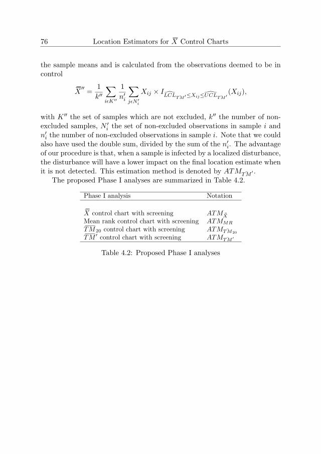
76 Location Estimators for X Control Charts
the sample means and is calculated from the observations deemed to be incontrol
X′′=
1
k′′∑iεK′′
1
n′i
∑jεN ′
i
Xij × ILCL ¯TM′≤Xij≤UCL ¯TM′ (Xij),
with K ′′ the set of samples which are not excluded, k′′ the number of non-excluded samples, N ′
i the set of non-excluded observations in sample i andn′i the number of non-excluded observations in sample i. Note that we couldalso have used the double sum, divided by the sum of the n′i. The advantageof our procedure is that, when a sample is infected by a localized disturbance,the disturbance will have a lower impact on the final location estimate whenit is not detected. This estimation method is denoted by ATM ¯TM
′ .The proposed Phase I analyses are summarized in Table 4.2.
Phase I analysis Notation
X control chart with screening ATM ¯XMean rank control chart with screening ATMMR
TM20 control chart with screening ATM ¯TM20
TM ′ control chart with screening ATM ¯TM ′
Table 4.2: Proposed Phase I analyses
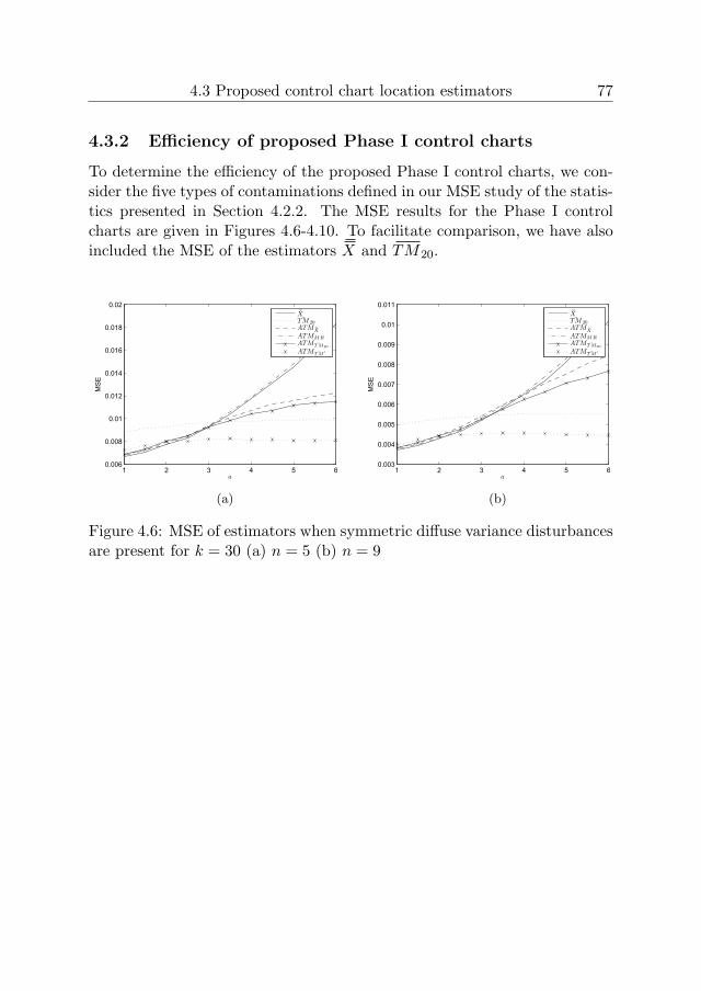
4.3 Proposed control chart location estimators 77
4.3.2 Efficiency of proposed Phase I control charts
To determine the efficiency of the proposed Phase I control charts, we con-sider the five types of contaminations defined in our MSE study of the statis-tics presented in Section 4.2.2. The MSE results for the Phase I controlcharts are given in Figures 4.6-4.10. To facilitate comparison, we have alsoincluded the MSE of the estimators X and TM20.
1 2 3 4 5 60.006
0.008
0.01
0.012
0.014
0.016
0.018
0.02
a
MS
E
¯X¯TM 20
ATM ¯X
ATMMR
ATM ¯T M20
ATM ¯T M′
(a)
1 2 3 4 5 60.003
0.004
0.005
0.006
0.007
0.008
0.009
0.01
0.011
a
MS
E
¯X¯TM 20
ATM ¯X
ATMMR
ATM ¯T M20
ATM ¯T M′
(b)
Figure 4.6: MSE of estimators when symmetric diffuse variance disturbancesare present for k = 30 (a) n = 5 (b) n = 9
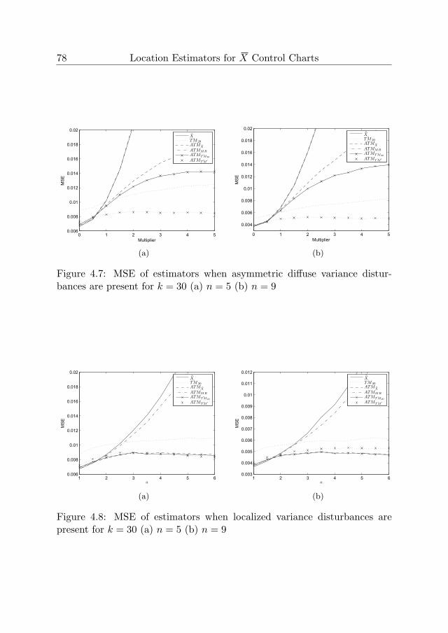
78 Location Estimators for X Control Charts
0 1 2 3 4 50.006
0.008
0.01
0.012
0.014
0.016
0.018
0.02
Multiplier
MS
E
¯X¯TM 20
ATM ¯X
ATMMR
ATM ¯T M20
ATM ¯T M′
(a)
0 1 2 3 4 5
0.004
0.006
0.008
0.01
0.012
0.014
0.016
0.018
0.02
MultiplierM
SE
¯X¯TM 20
ATM ¯X
ATMMR
ATM ¯T M20
ATM ¯T M′
(b)
Figure 4.7: MSE of estimators when asymmetric diffuse variance distur-bances are present for k = 30 (a) n = 5 (b) n = 9
1 2 3 4 5 60.006
0.008
0.01
0.012
0.014
0.016
0.018
0.02
a
MS
E
¯X¯TM 20
ATM ¯X
ATMMR
ATM ¯T M20
ATM ¯T M′
(a)
1 2 3 4 5 60.003
0.004
0.005
0.006
0.007
0.008
0.009
0.01
0.011
0.012
a
MS
E
¯X¯TM 20
ATM ¯X
ATMMR
ATM ¯T M20
ATM ¯T M′
(b)
Figure 4.8: MSE of estimators when localized variance disturbances arepresent for k = 30 (a) n = 5 (b) n = 9

4.3 Proposed control chart location estimators 79
0 2 4 6 8 10
0.01
0.02
0.03
0.04
0.05
0.06
0.07
0.08
b
MS
E
¯X¯TM 20
ATM ¯X
ATMMR
ATM ¯T M20
ATM ¯T M′
(a)
0 2 4 6 8 100
0.005
0.01
0.015
0.02
0.025
0.03
0.035
0.04
0.045
0.05
b
MS
E
¯X¯TM 20
ATM ¯X
ATMMR
ATM ¯T M20
ATM ¯T M′
(b)
Figure 4.9: MSE of estimators when diffuse mean disturbances are presentfor k = 30 (a) n = 5 (b) n = 9
0 1 2 3 4 5 60.005
0.01
0.015
0.02
0.025
MS
E
b
¯X¯TM 20
ATM ¯X
ATMMR
ATM ¯T M20
ATM ¯T M′
(a)
0 1 2 3 4 5 6
0.004
0.006
0.008
0.01
0.012
0.014
MS
E
b
¯X¯TM 20
ATM ¯X
ATMMR
ATM ¯T M20
ATM ¯T M′
(b)
Figure 4.10: MSE of estimators when localized mean disturbances arepresent for k = 30 (a) n = 5 (b) n = 9

80 Location Estimators for X Control Charts
The figures show that the standard Phase I analysis method, ATM ¯X ,
performs almost as well as X under normality when no contaminations arepresent and seems to be robust against localized variance disturbances. How-ever, the method loses efficiency in the other situations. Since X, the initialestimate of μ, is highly sensitive to disturbances, the Phase I limits are biasedand fail to identify the correct out-of-control samples.
The mean rank method, denoted by ATMMR, performs well under nor-mality and when there are localized mean disturbances. The reason is thatthis estimator screens for samples with a mean rank significantly higher thanthat of the other samples. On the other hand, ATMMR performs badly whendiffuse outliers are present. The mean rank is not influenced by occasionaloutliers so that samples containing only one outlier are not filtered out andhence are included in the calculation of the grand sample mean.
The third method, ATM ¯TM20, which uses the robust estimator TM20 to
construct a Phase I control chart, seems to be more efficient under normalitythan TM20 itself. The gain in efficiency can be explained by the use of anefficient estimator to obtain the final location estimate, once screening iscomplete. Thus, an efficient Phase I analysis does not require the use of anefficient estimator to construct the Phase I control chart.
The final method, ATM ¯TM′ , which first screens for localized disturbances
and then for occasional outliers, far outperforms all estimation methods. Themethod is particularly powerful in the presence of diffuse disturbances, be-cause its use of an individuals control chart in Phase I to identify singleoutliers increases the probability that such disturbances will be detected.For example, Figure 4.9 represents the situation where diffuse mean distur-bances are present. The efficiency of the estimator improves for high b valuesbecause the disturbances are more likely to fall outside the control limits andare therefore more likely to be detected.
4.4 Derivation of Phase II control limits
We now turn to the effect of the proposed location estimators on the Xcontrol chart performance in Phase II. The formulae for the X control limitswith estimated parameters are given by (1.4). For the Phase II control limits,we only estimate the in-control mean μ; we treat the in-control standarddeviation σ as known because we want to isolate the effect of estimating thelocation parameter. The factor Cn that is used to obtain accurate control

4.5 Control chart performance 81
limits when the process parameters are estimated is derived such that theprobability of a false signal equals the desired probability of a false signal.Except for the estimator X, Cn can not be obtained easily in analytic formand is therefore obtained by means of simulation. The factors are chosensuch that p is equal to 0.0027 under normality. 50,000 simulation runs areused. For k = 30 n = 5 and n = 9, the resulting factors are equal to 3.05for X, ATM ¯X , ATM ¯TM20
and ATM ¯TM′ ; 3.06 for X20 and TM and 3.07 for
M(X), M , HL, TM20 and ATMMR.
4.5 Control chart performance
In this section we evaluate the effect on X Phase II performance of theproposed location statistics and estimation methods based on Phase I controlcharting. We consider the same Phase I situations as those used to assess theMSE with a, b and the multiplier equal to 4 to simulate the contaminatedcases (see Section 4.2.2).
We use the unconditional run length distribution to assess performance.Specifically, we look at several characteristics of that distribution, namelythe average run length (ARL) and the standard deviation of the run length(SDRL). We also report the probability that one sample gives a signal (p).We compute these characteristics in an in-control and several out-of-controlsituations. We consider different shifts of size δσ in the mean, setting δequal to 0, 0.5, 1 and 2. The performance characteristics are obtained bysimulation. Section 4.5.1 describes the simulation method and Section 4.5.2gives simulation results identifying which control charts perform best in theuncontaminated and various contaminated situations.
4.5.1 Simulation procedure
The performance characteristics p and ARL for estimated control limits aredetermined by averaging the conditional characteristics, i.e. the character-istics for a given set of estimated control limits, over all possible valuesof the control limits. The corresponding definitions of p(Fi|μ), E(RL|μ),p = E(p(Fi|μ)) and ARL = E( 1
p(Fi|μ)) are obtained from (1.5)-(1.8), withall variables conditioned on μ rather than σ and σ = σ. These expectationsare obtained by simulation: numerous datasets are generated and for eachdataset p(Fi|μ) and E(RL|μ) are computed. By averaging these values we

82 Location Estimators for X Control Charts
obtain the unconditional values. The unconditional standard deviation isdetermined by (1.9).
Enough replications of the above procedure were performed to obtainsufficiently small relative estimated standard errors for p and ARL. Therelative standard error of the estimates is never higher than 0.60%.
4.5.2 Simulation results
First, we consider the situation where the process follows a normal distribu-tion and the Phase I data are not contaminated. We investigate the impactof the estimator used to estimate μ in Phase I. Table 4.3 presents p and theARL when the process mean equals μ + δσ. When the process is in con-trol (δ = 0), we want p to be as low as possible and ARL to be as high aspossible. In the out-of-control situation (δ �= 0), we want to achieve the op-posite. We can see that in the absence of any contamination (Table 4.3), theefficiency of the estimators is very similar. We can therefore conclude thatusing a more robust location estimator does not have a substantial impacton control chart performance in the uncontaminated situation.
The Phase II control charts based on the estimation methods M(X),
X20, TM20, ATM ¯X and ATMMR perform relatively well when localizeddisturbances are present, while the charts based on M , HL, TM and TM20
perform relatively well when diffuse disturbances are present (see Tables4.4-4.8).
The Phase II chart based on ATM ¯TM′ performs best: this chart is as
efficient as X in the uncontaminated normal situation and its performancedoes not change much when contaminations come into play. Moreover, thechart outperforms the other methods in all situations because it success-fully filters out both diffuse and localized disturbances. In the presence ofasymmetric disturbances, in particular, the added value of this estimationmethod is substantial.
When localized mean disturbances are present, we see a strange phe-nomenon for the X, M , HL and TM charts: the in-control ARL is lowerthan the out-of-control ARL for δ = 0.5. In other words, these charts aremore likely to give a signal in the in-control situation than in the out-of-control situation for δ = 0.5 and hence, in the presence of disturbances, arehighly ARL-biased (cf. Jensen et al. (2006)).

4.5 Control chart performance 83
p ARL and SDRLn μ δ = 0 δ = 0.5 δ = 1 δ = 2 δ = 0 δ = 0.5 δ = 1 δ = 2
5 X 0.0027 0.029 0.21 0.92 384 (392) 41.7 (49.4) 5.03 (4.90) 1.09 (0.32)M(X) 0.0027 0.028 0.21 0.91 390 (406) 46.2 (59.9) 5.31 (5.43) 1.10 (0.33)M 0.0027 0.028 0.21 0.91 392 (407) 45.9 (59.0) 5.29 (5.37) 1.10 (0.33)
X20 0.0027 0.028 0.21 0.92 391 (401) 43.3 (52.4) 5.14 (5.08) 1.09 (0.32)HL 0.0027 0.029 0.21 0.92 380 (389) 42.0 (50.4) 5.05 (4.94) 1.09 (0.32)TM 0.0027 0.028 0.21 0.92 390 (400) 43.4 (53.0) 5.14 (5.09) 1.09 (0.32)TM20 0.0027 0.028 0.21 0.92 396 (410) 45.3 (56.9) 5.26 (5.29) 1.09 (0.33)ATM ¯X
0.0027 0.029 0.21 0.92 383 (392) 41.8 (49.6) 5.04 (4.92) 1.09 (0.32)ATMMR 0.0027 0.029 0.21 0.92 383 (391) 41.5 (49.1) 5.04 (4.89) 1.09 (0.32)ATM ¯TM20
0.0027 0.029 0.21 0.92 382 (391) 41.8 (49.9) 5.04 (4.92) 1.09 (0.32)
ATM ¯TM′ 0.0027 0.029 0.21 0.92 381 (390) 42.0 (50.3) 5.06 (4.96) 1.09 (0.32)
9 X 0.0027 0.064 0.48 1.00 384 (393) 17.9 (20.0) 2.13 (1.62) 1.00 (0.043)M(X) 0.0027 0.063 0.47 1.00 390 (405) 19.5 (23.5) 2.19 (1.74) 1.00 (0.046)M 0.0027 0.063 0.47 1.00 390 (405) 19.5 (23.6) 2.19 (1.74) 1.00 (0.046)
X20 0.0027 0.063 0.48 1.00 391 (401) 18.5 (21.1) 2.15 (1.66) 1.00 (0.044)HL 0.0027 0.064 0.48 1.00 380 (389) 18.0 (20.4) 2.13 (1.63) 1.00 (0.043)TM 0.0027 0.063 0.48 1.00 390 (400) 18.6 (21.4) 2.16 (1.67) 1.00 (0.045)TM20 0.0027 0.062 0.47 1.00 395 (409) 19.3 (22.7) 2.18 (1.71) 1.00 (0.046)ATM ¯X
0.0027 0.064 0.48 1.00 382 (391) 17.9 (20.1) 2.13 (1.63) 1.00 (0.043)ATMMR 0.0027 0.064 0.48 1.00 382 (391) 17.9 (20.1) 2.13 (1.63) 1.00 (0.043)ATM ¯TM20
0.0027 0.064 0.48 1.00 382 (391) 18.0 (20.2) 2.13 (1.63) 1.00 (0.043)
ATM ¯TM′ 0.0027 0.064 0.48 1.00 380 (390) 18.0 (20.5) 2.13 (1.64) 1.00 (0.043)
Table 4.3: p, ARL and (in parentheses) SDRL of corrected limits undernormality for k = 30

84 Location Estimators for X Control Charts
p ARL and SDRLn μ δ = 0 δ = 0.5 δ = 1 δ = 2 δ = 0 δ = 0.5 δ = 1 δ = 2
5 X 0.0030 0.030 0.21 0.92 358 (375) 45.0 (60.9) 5.21 (5.44) 1.09 (0.33)M(X) 0.0029 0.029 0.21 0.91 375 (395) 48.4 (67.7) 5.41 (5.77) 1.10 (0.34)M 0.0028 0.029 0.21 0.91 387 (403) 46.5 (61.5) 5.34 (5.52) 1.10 (0.33)
X20 0.0028 0.029 0.21 0.92 376 (392) 45.1 (58.8) 5.23 (5.35) 1.09 (0.33)HL 0.0029 0.029 0.21 0.92 370 (383) 43.2 (54.5) 5.13 (5.15) 1.09 (0.32)TM 0.0027 0.029 0.21 0.92 384 (396) 44.2 (55.6) 5.19 (5.21) 1.09 (0.32)TM20 0.0027 0.028 0.21 0.91 390 (405) 46.0 (59.2) 5.29 (5.38) 1.10 (0.33)ATM ¯X
0.0030 0.030 0.21 0.92 362 (378) 44.4 (58.8) 5.18 (5.33) 1.09 (0.32)ATMMR 0.0030 0.030 0.21 0.92 357 (374) 45.1 (61.6) 5.21 (5.44) 1.09 (0.33)ATM ¯TM20
0.0029 0.030 0.21 0.92 364 (379) 44.3 (58.3) 5.18 (5.31) 1.09 (0.32)
ATM ¯TM′ 0.0028 0.029 0.21 0.92 375 (386) 42.7 (52.8) 5.09 (5.06) 1.09 (0.32)
9 X 0.0030 0.066 0.48 1.00 358 (375) 19.1 (24.0) 2.17 (1.73) 1.00 (0.045)M(X) 0.0030 0.065 0.47 1.00 371 (393) 20.6 (27.5) 2.23 (1.83) 1.00 (0.048)M 0.0028 0.063 0.47 1.00 386 (403) 19.8 (24.5) 2.20 (1.75) 1.00 (0.047)
X20 0.0029 0.064 0.48 1.00 373 (389) 19.4 (24.1) 2.18 (1.74) 1.00 (0.046)HL 0.0028 0.064 0.48 1.00 373 (385) 18.4 (21.5) 2.14 (1.66) 1.00 (0.044)TM 0.0027 0.063 0.48 1.00 384 (397) 18.8 (22.1) 2.16 (1.69) 1.00 (0.045)TM20 0.0027 0.063 0.47 1.00 391 (406) 19.4 (23.3) 2.19 (1.74) 1.00 (0.046)ATM ¯X
0.0030 0.066 0.48 1.00 358 (375) 19.2 (24.0) 2.17 (1.73) 1.00 (0.046)ATMMR 0.0031 0.066 0.48 1.00 356 (374) 19.1 (24.1) 2.17 (1.73) 1.00 (0.046)ATM ¯TM20
0.0030 0.066 0.48 1.00 360 (376) 19.0 (23.5) 2.16 (1.71) 1.00 (0.046)
ATM ¯TM′ 0.0028 0.064 0.48 1.00 375 (386) 18.3 (21.3) 2.14 (1.65) 1.00 (0.044)
Table 4.4: p, ARL and (in parentheses) SDRL of corrected limits whensymmetric variance disturbances are present for k = 30

4.5 Control chart performance 85
p ARL and SDRLn μ δ = 0 δ = 0.5 δ = 1 δ = 2 δ = 0 δ = 0.5 δ = 1 δ = 2
5 X 0.0076 0.012 0.12 0.82 233 (295) 143 (210) 12.8 (24.0) 1.23 (0.60)M(X) 0.0034 0.019 0.16 0.88 347 (378) 77.0 (110) 7.34 (8.26) 1.14 (0.41)M 0.0029 0.022 0.18 0.90 374 (395) 61.6 (82.4) 6.32 (6.73) 1.12 (0.37)
X20 0.0034 0.018 0.16 0.88 337 (366) 75.9 (103) 7.22 (7.91) 1.14 (0.41)HL 0.0033 0.020 0.17 0.89 340 (363) 67.3 (90.4) 6.73 (7.36) 1.13 (0.39)TM 0.0030 0.021 0.17 0.89 365 (384) 61.2 (69.2) 6.33 (6.61) 1.12 (0.37)TM20 0.0029 0.022 0.18 0.90 379 (398) 60.4 (78.7) 6.26 (6.56) 1.12 (0.37)ATM ¯X
0.0034 0.020 0.17 0.89 334 (359) 70.0 (95.0) 6.86 (7.51) 1.13 (0.39)ATMMR 0.0076 0.012 0.12 0.82 232 (294) 143 (209) 13.0 (26.7) 1.24 (0.61)ATM ¯TM20
0.0032 0.021 0.17 0.89 347 (367) 62.9 (82.9) 6.46 (6.84) 1.12 (0.38)
ATM ¯TM′ 0.0028 0.025 0.20 0.91 373 (385) 48.9 (60.2) 5.53 (5.55) 1.10 (0.34)
9 X 0.011 0.020 0.27 0.99 175 (239) 89.5 (148) 4.58 (6.42) 1.01 (0.12)M(X) 0.0044 0.035 0.36 0.99 299 (346) 42.1 (63.4) 3.04 (2.89) 1.01 (0.077)M 0.0031 0.048 0.42 1.00 366 (389) 26.8 (34.1) 2.51 (2.12) 1.00 (0.058)
X20 0.0047 0.033 0.35 0.99 280 (324) 42.7 (61.0) 3.09 (2.89) 1.01 (0.078)HL 0.0033 0.044 0.41 1.00 336 (358) 27.9 (33.9) 2.57 (2.15) 1.00 (0.059)TM 0.0031 0.046 0.42 1.00 356 (378) 26.4 (31.9) 2.51 (2.08) 1.00 (0.057)TM20 0.0030 0.047 0.42 1.00 368 (391) 26.8 (33.2) 2.52 (2.11) 1.00 (0.058)ATM ¯X
0.0046 0.035 0.36 0.99 282 (322) 39.6 (57.4) 2.98 (2.76) 1.01 (0.074)ATMMR 0.011 0.021 0.27 0.99 175 (240) 89.3 (148) 4.58 (6.41) 1.01 (0.12)ATM ¯TM20
0.0039 0.039 0.38 1.00 307 (339) 33.3 (44.1) 2.77 (2.44) 1.00 (0.066)
ATM ¯TM′ 0.0028 0.055 0.45 1.00 370 (383) 21.4 (24.9) 2.30 (1.83) 1.00 (0.050)
Table 4.5: p, ARL and (in parentheses) SDRL of corrected limits whenasymmetric variance disturbances are present for k = 30

86 Location Estimators for X Control Charts
p ARL and SDRLn μ δ = 0 δ = 0.5 δ = 1 δ = 2 δ = 0 δ = 0.5 δ = 1 δ = 2
5 X 0.0034 0.032 0.22 0.91 337 (361) 48.7 (73.0) 5.42 (6.09) 1.10 (0.34)M(X) 0.0028 0.029 0.21 0.91 382 (400) 47.4 (64.2) 5.40 (5.66) 1.10 (0.33)M 0.0037 0.033 0.22 0.91 335 (372) 57.2 (98.5) 5.90 (7.45) 1.11 (0.36)
X20 0.0028 0.029 0.21 0.92 382 (395) 44.3 (55.8) 5.21 (5.25) 1.09 (0.32)HL 0.0035 0.032 0.22 0.91 332 (358) 50.0 (76.8) 5.46 (6.22) 1.10 (0.34)TM 0.0035 0.032 0.22 0.91 338 (368) 52.3 (83.4) 5.62 (6.63) 1.10 (0.35)TM20 0.0028 0.029 0.21 0.91 387 (403) 46.6 (61.7) 5.36 (5.55) 1.10 (0.33)ATM ¯X
0.0028 0.029 0.21 0.92 371 (382) 43.1 (53.7) 5.12 (5.13) 1.09 (0.32)ATMMR 0.0033 0.031 0.22 0.92 342 (364) 47.7 (69.5) 5.34 (5.83) 1.10 (0.33)ATM ¯TM20
0.0028 0.029 0.21 0.92 371 (384) 42.9 (53.8) 5.12 (5.13) 1.09 (0.32)
ATM ¯TM′ 0.0028 0.029 0.21 0.92 372 (384) 43.0 (53.7) 5.11 (5.10) 1.09 (0.32)
9 X 0.0034 0.068 0.48 1.00 337 (362) 20.4 (28.6) 2.21 (1.84) 1.00 (0.048)M(X) 0.0028 0.064 0.47 1.00 381 (400) 19.9 (25.0) 2.21 (1.78) 1.00 (0.047)M 0.0038 0.069 0.47 1.00 332 (370) 24.0 (40.4) 2.32 (2.12) 1.00 (0.054)
X20 0.0028 0.064 0.48 1.00 382 (395) 18.9 (22.3) 2.17 (1.69) 1.00 (0.045)HL 0.0035 0.069 0.48 1.00 333 (359) 20.8 (30.1) 2.22 (1.88) 1.00 (0.049)TM 0.0035 0.068 0.48 1.00 338 (368) 21.8 (32.7) 2.25 (1.94) 1.00 (0.051)TM20 0.0028 0.063 0.47 1.00 385 (402) 19.7 (24.2) 2.20 (1.76) 1.00 (0.047)ATM ¯X
0.0028 0.065 0.48 1.00 372 (384) 18.4 (21.6) 2.15 (1.67) 1.00 (0.044)ATMMR 0.0033 0.068 0.48 1.00 342 (364) 20.0 (27.2) 2.20 (1.81) 1.00 (0.048)ATM ¯TM20
0.0028 0.065 0.48 1.00 372 (384) 18.4 (21.7) 2.15 (1.67) 1.00 (0.044)
ATM ¯TM′ 0.0029 0.065 0.48 1.00 368 (381) 18.6 (22.2) 2.15 (1.68) 1.00 (0.045)
Table 4.6: p, ARL and (in parentheses) SDRL of corrected limits whenlocalized variance disturbances are present for k = 30
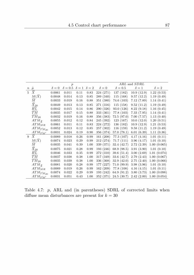
4.5 Control chart performance 87
p ARL and SDRLn μ δ = 0 δ = 0.5 δ = 1 δ = 2 δ = 0 δ = 0.5 δ = 1 δ = 2
5 X 0.0061 0.011 0.11 0.83 224 (271) 137 (182) 10.9 (12.9) 1.22 (0.53)M(X) 0.0048 0.014 0.13 0.85 289 (340) 115 (168) 9.57 (12.2) 1.19 (0.49)M 0.0033 0.019 0.16 0.88 351 (380) 74.6 (103) 7.12 (7.89) 1.14 (0.41)
X20 0.0049 0.013 0.13 0.85 271 (316) 115 (158) 9.52 (11.2) 1.19 (0.49)HL 0.0042 0.015 0.14 0.86 290 (326) 93.0 (126) 8.22 (9.18) 1.16 (0.45)TM 0.0035 0.017 0.15 0.88 333 (361) 77.8 (103) 7.33 (7.95) 1.14 (0.41)TM20 0.0032 0.019 0.16 0.88 356 (383) 72.5 (97.0) 7.00 (7.57) 1.13 (0.40)ATM ¯X
0.0055 0.012 0.12 0.84 245 (392) 123 (167) 10.0 (12.0) 1.20 (0.51)ATMMR 0.0061 0.011 0.11 0.83 224 (272) 136 (182) 10.9 (12.9) 1.21 (0.53)ATM ¯TM20
0.0052 0.013 0.12 0.85 257 (302) 116 (159) 9.58 (11.2) 1.19 (0.49)
ATM ¯TM′ 0.0031 0.024 0.19 0.90 356 (374) 57.0 (78.1) 6.01 (6.39) 1.11 (0.36)
9 X 0.0089 0.018 0.26 0.99 161 (208) 77.3 (107) 4.17 (4.16) 1.01 (0.11)M(X) 0.0074 0.023 0.29 0.99 212 (274) 71.7 (111) 3.96 (4.17) 1.01 (0.10)M 0.0035 0.041 0.39 1.00 339 (371) 32.4 (42.7) 2.72 (2.39) 1.00 (0.065)
X20 0.0075 0.021 0.28 0.99 193 (246) 68.9 (98.5) 3.91 (3.90) 1.01 (0.10)HL 0.0046 0.033 0.35 0.99 272 (310) 39.6 (51.4) 3.00 (2.69) 1.01 (0.074)TM 0.0037 0.038 0.38 1.00 317 (349) 33.6 (42.7) 2.79 (2.43) 1.00 (0.067)TM20 0.0035 0.039 0.38 1.00 336 (368) 32.9 (42.0) 2.75 (2.40) 1.00 (0.066)ATM ¯X
0.0081 0.020 0.28 0.99 177 (227) 71.0 (99.9) 3.98 (3.96) 1.01 (0.10)ATMMR 0.0089 0.019 0.26 0.99 162 (209) 77.8 (108) 4.16 (4.15) 1.01 (0.11)ATM ¯TM20
0.0074 0.022 0.29 0.99 193 (242) 64.9 (91.2) 3.80 (3.73) 1.00 (0.098)
ATM ¯TM′ 0.0031 0.051 0.43 1.00 352 (371) 24.5 (30.7) 2.42 (2.00) 1.00 (0.054)
Table 4.7: p, ARL and (in parentheses) SDRL of corrected limits whendiffuse mean disturbances are present for k = 30

88 Location Estimators for X Control Charts
p ARL and SDRLn μ δ = 0 δ = 0.5 δ = 1 δ = 2 δ = 0 δ = 0.5 δ = 1 δ = 2
5 X 0.017 0.0034 0.046 0.70 72.3 (87.5) 329 (351) 25.0 (28.8) 1.45 (0.83)M(X) 0.0031 0.021 0.17 0.89 366 (389) 66.0 (89.3) 6.62 (7.15) 1.13 (0.38)M 0.017 0.0033 0.045 0.69 80.1 (105) 343 (372) 27.3 (33.6) 1.47 (0.86)
X20 0.0030 0.020 0.17 0.89 360 (379) 64.8 (81.8) 6.57 (6.81) 1.13 (0.38)HL 0.017 0.0034 0.047 0.70 72.8 (89.3) 327 (350) 25.2 (29.2) 1.45 (0.83)TM 0.017 0.0033 0.046 0.69 75.6 (94.4) 337 (362) 26.0 (30.7) 1.46 (0.84)TM20 0.0031 0.019 0.16 0.89 360 (385) 70.4 (92.0) 6.89 (7.32) 1.13 (0.40)ATM ¯X
0.0028 0.026 0.20 0.91 373 (385) 47.5 (49.1) 5.44 (5.47) 1.10 (0.33)ATMMR 0.0028 0.029 0.21 0.92 378 (388) 42.1 (50.9) 5.08 (4.99) 1.09 (0.32)ATM ¯TM20
0.0028 0.029 0.21 0.92 378 (388) 42.8 (52.1) 5.12 (5.07) 1.09 (0.32)
ATM ¯TM′ 0.0028 0.029 0.21 0.92 375 (386) 43.4 (53.4) 5.14 (5.11) 1.09 (0.32)
9 X 0.035 0.0039 0.11 0.96 34.3 (30.7) 293 (321) 10.1 (10.7) 1.04 (0.22)M(X) 0.0031 0.048 0.42 1.00 366 (389) 26.8 (34.3) 2.51 (2.12) 1.00 (0.058)M 0.034 0.0039 0.11 0.95 37.9 (48.5) 308 (346) 10.8 (12.3) 1.05 (0.23)
X20 0.0030 0.046 0.41 1.00 359 (379) 26.3 (31.5) 2.51 (2.07) 1.00 (0.057)HL 0.035 0.0039 0.11 0.96 34.5 (40.8) 293 (322) 10.1 (10.9) 1.05 (0.22)TM 0.034 0.0039 0.11 0.96 35.7 (43.1) 301 (333) 10.4 (11.4) 1.05 (0.22)TM20 0.0031 0.044 0.41 1.00 361 (385) 28.4 (35.4) 2.58 (2.18) 1.00 (0.060)ATM ¯X
0.0029 0.055 0.45 1.00 366 (380) 21.7 (25.9) 2.30 (1.85) 1.00 (0.050)ATMMR 0.0028 0.064 0.48 1.00 377 (387) 18.2 (20.9) 2.14 (1.64) 1.00 (0.044)ATM ¯TM20
0.0028 0.063 0.48 1.00 378 (388) 18.4 (21.1) 2.15 (1.66) 1.00 (0.044)
ATM ¯TM′ 0.0028 0.063 0.48 1.00 376 (386) 18.6 (21.5) 2.16 (1.67) 1.00 (0.044)
Table 4.8: p, ARL and (in parentheses) SDRL of corrected limits whenlocalized mean disturbances are present for k = 30

4.6 Concluding remarks 89
4.6 Concluding remarks
In this chapter we have considered several Phase I estimators of the locationparameter for use in establishing X Phase II control chart limits. The col-lection includes robust estimators proposed in the existing literature as wellas several Phase I analyses, which apply a control chart retrospectively tostudy a historical dataset. The estimators have been evaluated under variouscircumstances: the uncontaminated situation and various situations contam-inated with diffuse symmetric and asymmetric variance disturbances, local-ized variance disturbances, diffuse mean disturbances and localized meandisturbances.
The standard methods suffer from a number of problems. Estimatorsthat are based on the principle of trimming individual observations (e.g. Mand TM) perform reasonably well when there are diffuse disturbances butnot when localized disturbances are present. In the latter situation, estima-tors that are based on the principle of trimming samples (e.g. M(X) and
X20) are efficient. All of these methods are biased when there are asymmet-ric disturbances, as the trimming principle does not take into account theasymmetry of the disturbance.
A Phase I analysis, using a control chart to study a historical datasetretrospectively and trim the data adaptively, does take into account thedistribution of the disturbance and is therefore very suitable for use duringthe estimation of μ. However, the standard method based on the X PhaseI control chart has certain limitations. First, the initial estimate, X, is verysensitive to outliers so that the Phase I limits are biased. As a consequence,the wrong data samples are often filtered out. Second, the sample meanis usually plotted on the Phase I control chart, which makes it difficultto detect outliers in individual observations. Moreover, deleting the entiresample instead of the single outlier reduces efficiency.
To address the problems encountered in the standard Phase I analysis, wehave proposed a new type of Phase I analysis. The initial estimate of μ for thePhase I control chart is based on a trimmed version of the trimean, namelyTM20, and a subsequent procedure for both sample screening and outlierscreening (resulting in ATM ¯TM
′). The proposed method is efficient undernormality and far outperforms the existing methods when disturbances arepresent. Consequently, ATM ¯TM
′ is a very effective method for estimating μin the limits used to construct the X Phase II chart.


Chapter 5
A Robust X Control Chart
5.1 Introduction
This chapter studies alternative standard deviation estimators that serveas a basis to determine the X control chart limits used for real-time pro-cess monitoring (Phase II). Several existing (robust) estimation methods areconsidered. In addition, we propose a new estimation method based on aPhase I analysis, whereby a control chart is used to identify disturbances ina dataset retrospectively. The method constructs a Phase I control chart de-rived from the trimmed mean of the sample interquartile ranges in order toidentify out-of-control data. An efficient estimator, namely the mean of thesample standard deviations, is used to obtain the final standard deviationestimate from the remaining data. The estimation methods are evaluatedin terms of their MSE and their effects on the performance of the X PhaseII control chart. It is shown that the newly proposed estimation method isefficient under normality and performs substantially better than standardmethods when disturbances are present in Phase I.
The chapter is structured as follows. We first present the estimationmethods for the standard deviation and assess the MSE of the estimators.In the following sections, we present the design schemes for the X Phase IIcontrol chart and derive the control limits. Next, we describe the simula-tion procedure and present the effect of the proposed methods on Phase IIperformance. The final section offers some recommendations.
91
92 A Robust X Control Chart
5.2 Proposed Phase I estimators
We analyze various types of standard deviation estimators and comparethem under various types of disturbances. The next two sections introducethe standard deviation and location estimators respectively, while the thirdsection presents the MSE of the standard deviation estimators.
5.2.1 Standard deviation estimators
We again denote the Phase I data by Xij , i = 1, 2, ..., k and j = 1, 2, ..., n.The Xij ’s are assumed to be independent and N(μ, σ2) distributed. Wedenote by Xi,(v), v = 1, 2, ..., n, the v-th order statistic in sample i. We lookat several robust estimators proposed in the existing literature and introducea new method incorporating a Phase I control chart.
We consider the traditional estimators of the standard deviation, namelythe mean of the sample standard deviations S (see (2.2)), the mean of thesample ranges R (see (2.5)) and the mean of the sample interquartile ranges(see (2.6)). We saw in Chapter 2 that S is slightly less efficient under nor-mality than the pooled sample standard deviation S.
Rocke (1989) proposed the trimmed mean of the sample interquartileranges
IQRα =1
k − 2�kα�×[ k−�kα�∑v=�kα�+1
IQR(v)
],
where IQR(v) denotes the v-th ordered value of the sample interquartileranges. We consider the 20% trimmed mean of the sample interquartileranges, which trims the ten smallest and the ten largest sample interquartileranges when k = 50 and the twenty smallest and the twenty largest sampleinterquartile ranges when k = 100. An unbiased estimator of σ is given byIQR20/d ¯IQR20
, where d ¯IQR20is a normalizing constant. The value of this
constant is 0.925 for n = 5 and 1.108 for n = 9.
We also evaluate a robust estimator proposed by Tatum (1997). Thisestimator is defined in (2.11).
We now present a new estimation method based on the principle of PhaseI control charting. We build a Phase I control chart using a robust estimatorfor the standard deviation, namely IQR20. A disadvantage of this estimatoris that it is not very efficient under normality. To address this, we useIQR20 to construct the Phase I limits with which we screen the estimation
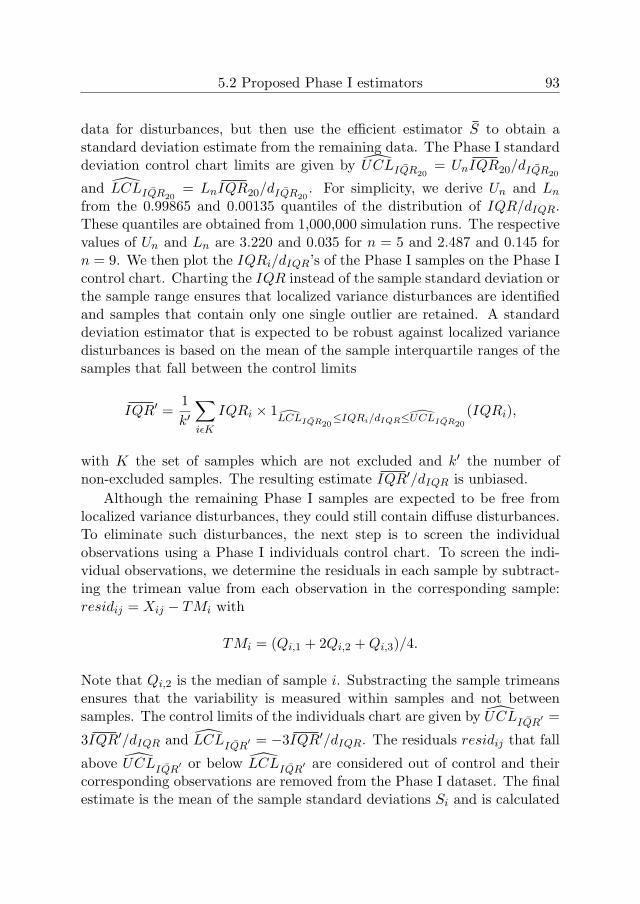
5.2 Proposed Phase I estimators 93
data for disturbances, but then use the efficient estimator S to obtain astandard deviation estimate from the remaining data. The Phase I standarddeviation control chart limits are given by UCL ¯IQR20
= UnIQR20/d ¯IQR20
and LCL ¯IQR20= LnIQR20/d ¯IQR20
. For simplicity, we derive Un and Ln
from the 0.99865 and 0.00135 quantiles of the distribution of IQR/dIQR.These quantiles are obtained from 1,000,000 simulation runs. The respectivevalues of Un and Ln are 3.220 and 0.035 for n = 5 and 2.487 and 0.145 forn = 9. We then plot the IQRi/dIQR’s of the Phase I samples on the Phase Icontrol chart. Charting the IQR instead of the sample standard deviation orthe sample range ensures that localized variance disturbances are identifiedand samples that contain only one single outlier are retained. A standarddeviation estimator that is expected to be robust against localized variancedisturbances is based on the mean of the sample interquartile ranges of thesamples that fall between the control limits
IQR′ =1
k′∑iεK
IQRi × 1LCL ¯IQR20
≤IQRi/dIQR≤UCL ¯IQR20
(IQRi),
with K the set of samples which are not excluded and k′ the number ofnon-excluded samples. The resulting estimate IQR′/dIQR is unbiased.
Although the remaining Phase I samples are expected to be free fromlocalized variance disturbances, they could still contain diffuse disturbances.To eliminate such disturbances, the next step is to screen the individualobservations using a Phase I individuals control chart. To screen the indi-vidual observations, we determine the residuals in each sample by subtract-ing the trimean value from each observation in the corresponding sample:residij = Xij − TMi with
TMi = (Qi,1 + 2Qi,2 +Qi,3)/4.
Note that Qi,2 is the median of sample i. Substracting the sample trimeansensures that the variability is measured within samples and not betweensamples. The control limits of the individuals chart are given by UCL ¯IQR
′ =
3IQR′/dIQR and LCL ¯IQR′ = −3IQR′/dIQR. The residuals residij that fall
above UCL ¯IQR′ or below LCL ¯IQR
′ are considered out of control and theircorresponding observations are removed from the Phase I dataset. The finalestimate is the mean of the sample standard deviations Si and is calculated

94 A Robust X Control Chart
from the observations deemed to be in control
S′ =1
k∧∑iεK∧
Si({Xij × 1LCL ¯IQR′≤residij≤UCL ¯IQR′})(Xij),
with K∧ the set of samples which are not excluded and k∧ the number ofnon-excluded samples. The normalizing constant is 0.980 for n = 5 and0.984 for n = 9. This adaptively trimmed standard deviation is denoted byATS.
The proposed standard deviation estimators are summarized in Table5.1.
Estimator Notation
Mean of sample standard deviations SMean of sample ranges RMean of sample interquartile ranges IQR20% trimmed mean of sample interquartile ranges IQR20
Tatum’s estimator D7IQR′ control chart with screening ATS
Table 5.1: Proposed standard deviation estimators
5.2.2 Location estimator
The above standard deviation estimators are used to construct the X PhaseII control limits. To ensure a fair comparison, we use the same locationestimator in each case. The location estimation method uses a proceduresimilar to ATS above. Chapter 4 showed that this procedure performs betterthan the standard procedures based on estimators such as the mean, median,trimmed mean and Hodges-Lehmann. Again, the procedure consists of twosteps.
In the first step we determine a location estimator that is robust againstboth localized and diffuse mean disturbances, namely the 20% trimmed meanof the sample trimeans
TMα =1
k − 2�kα�×[ k−�kα�∑v=�kα�+1
TM(v)
].

5.2 Proposed Phase I estimators 95
Note that we start with the entire dataset. The respective upper and lowercontrol limits for the sample location are given by UCL ¯TM20
= TM20 +
3σ/√n and LCL ¯TM20
= TM20 − 3σ/√n, where σ is estimated by the cor-
responding standard deviation estimator from Table 5.1. We then plot theTMi’s of the Phase I samples on the control chart. Charting the TMi’sinstead of the Xi’s ensures that localized disturbances are identified andsamples that contain only one single outlier are retained. A location estima-tor that is expected to be robust against localized mean disturbances is themean of the sample trimeans of the samples that fall between the controllimits
TM ′ =1
k∗∑iεK∗
TMi × 1LCL ¯TM20
≤TMi≤UCL ¯TM20
(TMi),
with K∗ the set of samples which are not excluded and k∗ the number ofnon-excluded samples.
Although the remaining Phase I samples are expected to be free fromlocalized mean disturbances, they could still contain diffuse disturbances.To eliminate such disturbances, the next step is to screen the individualobservations using a Phase I individuals control chart with respective upperand lower control limits given by UCL ¯TM
′ = TM ′ + 3σ and LCL ¯TM′ =
TM ′ − 3σ, where σ is estimated by the corresponding standard deviationestimator from Table 5.1. The observations Xij that fall above UCL ¯TM
′ or
below LCL ¯TM′ are considered out of control and removed from the Phase I
dataset. The final estimate is based on the mean of the sample means andis calculated from the observations deemed to be in control
X′=
1
k′′∑iεK′′
1
n′i
∑jεN ′
i
Xij × 1LCL ¯TM′≤Xij≤UCL ¯TM′ (Xij),
with K ′′ the samples which are not excluded, k′′ the number of non-excludedsamples, N ′
i the non-excluded observations in sample i and n′i the numberof non-excluded observations in sample i.
5.2.3 Efficiency of proposed standard deviation estimators
We again use the MSE of the proposed standard deviation estimators toevaluate their efficiency. The MSE is estimated as
MSE =1
N
N∑i=1
(σi − σ
)2
,
96 A Robust X Control Chart
where σi is the value of the unbiased estimate in the i-th simulation run andN is the number of simulation runs. We consider the uncontaminated case,i.e. the situation where all the Xij ’s are from the N(0, 1) distribution, aswell as four types of disturbances (see Section 2.2.2).
The MSE is obtained for k = 50, 100 subgroups of sizes n = 5, 9. Thenumber of simulation runs N is equal to 50,000.

5.2 Proposed Phase I estimators 97
1 2 3 4 5 60
0.005
0.01
0.015
0.02
0.025
0.03
a
MS
E
S
R¯IQR¯IQR
20
D7
ATS
(a)
1 2 3 4 5 60
0.002
0.004
0.006
0.008
0.01
0.012
0.014
0.016
0.018
0.02
a
MS
E
S
R¯IQR¯IQR
20
D7
ATS
(b)
1 2 3 4 5 60
0.005
0.01
0.015
a
MS
E
S
R¯IQR¯IQR
20
D7
ATS
(c)
1 2 3 4 5 60
0.001
0.002
0.003
0.004
0.005
0.006
0.007
0.008
0.009
0.01
a
MS
E
S
R¯IQR¯IQR
20
D7
ATS
(d)
Figure 5.1: MSE of estimators when symmetric diffuse variance disturbancesare present. (a) n = 5, k = 50 (b) n = 5, k = 100 (c) n = 9, k = 50 (d)n = 9, k = 100

98 A Robust X Control Chart
0 1 2 3 4 50
0.005
0.01
0.015
0.02
0.025
a
MS
E
S
R¯IQR¯IQR
20
D7
ATS
(a)
0 1 2 3 4 50
0.005
0.01
0.015
a
MS
E
S
R¯IQR¯IQR
20
D7
ATS
(b)
0 1 2 3 4 50
0.001
0.002
0.003
0.004
0.005
0.006
0.007
0.008
0.009
0.01
a
MS
E
S
R¯IQR¯IQR
20
D7
ATS
(c)
0 1 2 3 4 50
0.001
0.002
0.003
0.004
0.005
0.006
0.007
0.008
a
MS
E
S
R¯IQR¯IQR
20
D7
ATS
(d)
Figure 5.2: MSE of estimators when asymmetric diffuse variance distur-bances are present. (a) n = 5, k = 50 (b) n = 5, k = 100 (c) n = 9, k = 50(d) n = 9, k = 100

5.2 Proposed Phase I estimators 99
1 2 3 4 5 60
0.005
0.01
0.015
0.02
0.025
0.03
a
MS
E
S
R¯IQR¯IQR
20
D7
ATS
(a)
1 2 3 4 5 60
0.002
0.004
0.006
0.008
0.01
0.012
0.014
0.016
0.018
0.02
a
MS
E
S
R¯IQR¯IQR
20
D7
ATS
(b)
1 2 3 4 5 60
0.005
0.01
0.015
a
MS
E
S
R¯IQR¯IQR
20
D7
ATS
(c)
1 2 3 4 5 60
0.001
0.002
0.003
0.004
0.005
0.006
0.007
0.008
0.009
0.01
a
MS
E
S
R¯IQR¯IQR
20
D7
ATS
(d)
Figure 5.3: MSE of estimators when localized variance disturbances arepresent. (a) n = 5, k = 50 (b) n = 5, k = 100 (c) n = 9, k = 50 (d)n = 9, k = 100

100 A Robust X Control Chart
0 2 4 6 8 100
0.005
0.01
0.015
0.02
0.025
0.03
0.035
0.04
b
MS
E
S
R¯IQR¯IQR
20
D7
ATS
(a)
0 2 4 6 8 100
0.005
0.01
0.015
0.02
0.025
MS
E
b
S
R¯IQR¯IQR
20
D7
ATS
(b)
0 2 4 6 8 100
0.005
0.01
0.015
0.02
0.025
b
MS
E
S
R¯IQR¯IQR
20
D7
ATS
(c)
0 2 4 6 8 100
0.005
0.01
0.015
0.02
0.025
b
MS
E
S
R¯IQR¯IQR
20
D7
ATS
(d)
Figure 5.4: MSE of estimators when diffuse mean disturbances are present.(a) n = 5, k = 50 (b) n = 5, k = 100 (c) n = 9, k = 50 (d) n = 9, k = 100

5.3 Derivation of Phase II control limits 101
Figures 5.1-5.4 show the MSE of the proposed estimators. The followingresults can be observed. The standard estimators S and R are not robustagainst either localized or diffuse disturbances. The IQR is less efficient un-der normality when there are no contaminations, but performs reasonablywell when there are diffuse disturbances. The reason why IQR performs sowell in these situations is that it trims the highest and lowest observations ineach sample. However, this estimator remains biased when there are asym-metric diffuse disturbances because the trimming method does not take thedistribution of the contaminations into account. Furthermore, this estima-tor is not efficient when there are localized variance disturbances as it trimsonly the observations within the sample instead of the sample interquartileranges.
An estimator that combines within-sample and between-sample trim-ming, namely IQR20, performs reasonably well for all types of contamina-tions. However, its efficiency is relatively low under normality. D7 is efficientunder normality as well as for contaminated data but relatively less so whenthe contamination consists of localized variance disturbances.
The estimator ATS is slightly less efficient under normality than thestandard estimators, but much more robust than IQR and IQR20. More-over, it shows outstanding performance when contaminations are present.We can therefore conclude that this estimator effectively filters out extremeobservations.
5.3 Derivation of Phase II control limits
We now turn to the effect of the proposed estimators on the performanceof the X Phase II control chart. The formulae for the X control limitswith estimated parameters are given by (1.4). The factor Cn that is used toobtain accurate control limits when the process parameters are estimated isderived such that the probability of a false signal equals the chosen type Ierror probability p. The factors can not be obtained easily in analytic form.Therefore, they are obtained by means of simulation. The chosen type Ierror probability p is 0.0027. 50,000 simulation runs are used. The resultingfactors are presented in Table 5.2.

102 A Robust X Control Chart
Factors for control limitsn = 5 n = 9
σ k = 50 k = 100 k = 50 k = 100
S 3.065 3.030 3.050 3.025R 3.070 3.035 3.055 3.025IQR 3.125 3.060 3.080 3.040IQR20 3.155 3.080 3.090 3.045D7 3.070 3.035 3.050 3.025ATS 3.085 3.040 3.055 3.025
Table 5.2: Factors Cn to determine Phase II control limits
5.4 Control chart performance
In this section we evaluate the effect on X Phase II performance of theproposed standard deviation estimators. We consider the same Phase I sit-uations as those used to assess the MSE with a, b and the multiplier equalto 4 to simulate the contaminated cases (see Section 5.2.3).
The performance of the Phase II control charts is assessed in terms of theunconditional p and ARL as well as the conditional ARL. The conditionalARL values express the ARL values for the control limits associated withthe 2.5% and 95.7% quantiles of p in the in-control situation. We considerdifferent shifts of size δσ in the mean in Phase II, namely δ equal to 0,0.25, 0.5 and 1. The performance characteristics are obtained by simulation.Sections 5.4.1 and 5.4.2 describe the simulation procedure and simulationresults, enabling a comparison of control charts across the uncontaminatedand contaminated situations.
5.4.1 Simulation procedure
The performance characteristics p and ARL for estimated control limits aredetermined by averaging the conditional characteristics, i.e. the character-istics for a given set of estimated control limits, over all possible values ofthe control limits. The corresponding definitions of p(Fi|μ, σ), E(RL|μ, σ),p = E(p(Fi|μ, σ)) and ARL = E( 1
p(Fi|μ,σ)) are obtained from (1.5)-(1.8),where the variables are conditioned on μ and σ. These expectations are ob-

5.4 Control chart performance 103
tained by simulation: numerous datasets are generated and for each datasetp(Fi|μ, σ) and E(RL|μ, σ) are computed. By averaging these values we ob-tain the unconditional values.
Enough replications of the above procedure were performed to obtainsufficiently small relative estimated standard errors for p and ARL. Therelative standard error of the estimates is never higher than 0.80%.
5.4.2 Simulation results
The performance metrics are obtained in the in-control situation as well asin the out-of-control situation. When the process is in control (δ = 0), wewant p to be as low as possible and ARL to be as high as possible. In theout-of-control situation (δ �= 0), we want to achieve the opposite.
Tables 5.3 and 5.4 show the results for the X Phase II charts undernormality. In this case we have estimated both the in-control μ and σ inPhase I. Unlike the X Phase II performance presented in Chapter 4, whereonly the mean was estimated to isolate the effect of location estimation,the ARL values are much higher than the desired 370. Thus, estimatingthe process standard deviation as well as the mean has substantially moreimpact on the X Phase II control chart than only estimating the processmean.
The conditional ARL values are presented in parentheses. The first valuerepresents the ARL for the control limits associated with the 97.5% quantileof the simulated p in the in-control situation, while the second value repre-sents the ARL for the control limits associated with the 2.5% quantile of thesimulated p in the in-control situation. The results show that the conditionalARL values vary quite strongly, even when k equals 100.
In the absence of any contamination, the charts based on S, R, D7 andATS show comparable performance. The charts based on IQR and IQR20
are less powerful under normality.
The analysis shows that, when there are disturbances in the Phase Idata, the performance of all charts changes considerably: there is a sizeabledecrease in p and increase in ARL. In other words, when the Phase I data arecontaminated, shifts in the process mean are less quickly detected. Whensymmetric disturbances are present (Tables 5.5 and 5.6), their impact is thesmallest for the charts based on IQR, IQR20, D7 and ATS. These chartsare also least affected when there are asymmetric disturbances (Tables 5.7and 5.8). Both tables show that the chart based on ATS outperforms the

104 A Robust X Control Chart
others.When there are localized disturbances (Tables 5.9 and 5.10), the charts
based on the estimators D7 and ATS perform best, the reason being thatthese charts trim extreme samples. Finally, in the case of diffuse meandisturbances (Tables 5.11 and 5.12), the charts based on IQR20, D7 andATS perform better than the other charts.
Overall, the ATS chart performs best. Under normality, the chart essen-tially matches the performance of the standard charts based on S and R and,in the presence of any contamination, the chart outperforms the alternatives.

5.5 Concluding remarks 105
5.5 Concluding remarks
We have analyzed several estimation methods for the standard deviation pa-rameter and compared the MSE of the estimators under a range of circum-stances: the uncontaminated situation and various situations contaminatedwith diffuse symmetric and asymmetric variance disturbances, localized vari-ance disturbances and diffuse mean disturbances. We have also investigatedthe effect of estimating the standard deviation on X Phase II control chartperformance when the methods are used to determine the Phase II limits.
One of the proposed methods has allowed us to address certain problemsexhibited by the standard methods. Estimators that trim observations (e.g.IQR) perform reasonably well when there are diffuse disturbances but notwhen there are localized disturbances. In the latter case, estimators thatinclude a method to trim sample statistics (e.g. IQR20) are efficient. But allsuch methods are biased when disturbances are asymmetric, as the trimmingdoes not take asymmetry into account.
A Phase I analysis - using a control chart to study a historical datasetretrospectively and trim the data adaptively - does consider the distributionof the disturbance, making it well-suited to the estimation of σ. In this chap-ter we have proposed a new type of Phase I analysis. The initial estimate ofσ for the Phase I control chart is given by an estimator that is robust againstboth diffuse and localized disturbances, namely IQR20. We have shown thatthis estimator is not very efficient under normality. However, when IQR20
is only used to construct the Phase I control chart limits, and when thestandard estimation method S is used to determine the final estimate of σafter screening, the resulting estimator (ATS) is efficient under normality.Moreover, ATS outperforms the other estimation methods when there arecontaminations. It is therefore a suitable method for determining the valueof σ in the X Phase II control chart limits.
Note that in Chapter 3 we evaluated the standard deviation estimatorMDi,s, whose performance essentially matches that of ATS. The differenceis that, in the case of ATS, the estimators used in Phase I and Phase IIare not the same. The estimator used in Phase I is very robust so that thePhase I control limits better represent the in-control state of the process. Asa result, only one iteration of the screening step is required. We think that,on the whole, ATS is of more practical use.
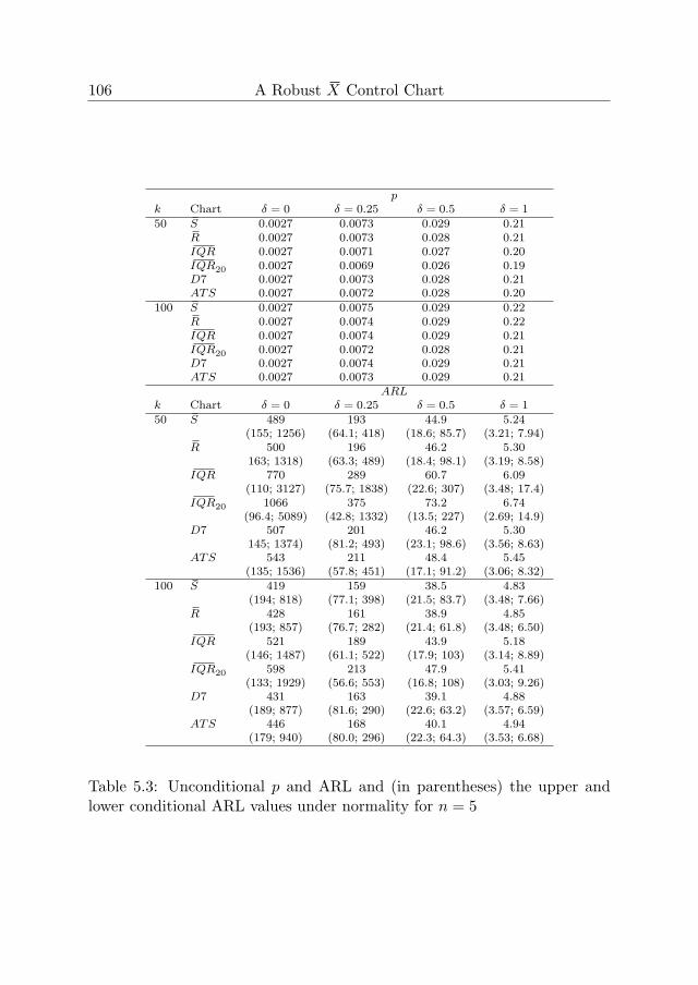
106 A Robust X Control Chart
pk Chart δ = 0 δ = 0.25 δ = 0.5 δ = 1
50 S 0.0027 0.0073 0.029 0.21R 0.0027 0.0073 0.028 0.21IQR 0.0027 0.0071 0.027 0.20IQR20 0.0027 0.0069 0.026 0.19D7 0.0027 0.0073 0.028 0.21ATS 0.0027 0.0072 0.028 0.20
100 S 0.0027 0.0075 0.029 0.22R 0.0027 0.0074 0.029 0.22IQR 0.0027 0.0074 0.029 0.21IQR20 0.0027 0.0072 0.028 0.21D7 0.0027 0.0074 0.029 0.21ATS 0.0027 0.0073 0.029 0.21
ARLk Chart δ = 0 δ = 0.25 δ = 0.5 δ = 1
50 S 489 193 44.9 5.24(155; 1256) (64.1; 418) (18.6; 85.7) (3.21; 7.94)
R 500 196 46.2 5.30163; 1318) (63.3; 489) (18.4; 98.1) (3.19; 8.58)
IQR 770 289 60.7 6.09(110; 3127) (75.7; 1838) (22.6; 307) (3.48; 17.4)
IQR20 1066 375 73.2 6.74(96.4; 5089) (42.8; 1332) (13.5; 227) (2.69; 14.9)
D7 507 201 46.2 5.30145; 1374) (81.2; 493) (23.1; 98.6) (3.56; 8.63)
ATS 543 211 48.4 5.45(135; 1536) (57.8; 451) (17.1; 91.2) (3.06; 8.32)
100 S 419 159 38.5 4.83(194; 818) (77.1; 398) (21.5; 83.7) (3.48; 7.66)
R 428 161 38.9 4.85(193; 857) (76.7; 282) (21.4; 61.8) (3.48; 6.50)
IQR 521 189 43.9 5.18(146; 1487) (61.1; 522) (17.9; 103) (3.14; 8.89)
IQR20 598 213 47.9 5.41(133; 1929) (56.6; 553) (16.8; 108) (3.03; 9.26)
D7 431 163 39.1 4.88(189; 877) (81.6; 290) (22.6; 63.2) (3.57; 6.59)
ATS 446 168 40.1 4.94(179; 940) (80.0; 296) (22.3; 64.3) (3.53; 6.68)
Table 5.3: Unconditional p and ARL and (in parentheses) the upper andlower conditional ARL values under normality for n = 5

5.5 Concluding remarks 107
pk Chart δ = 0 δ = 0.25 δ = 0.5 δ = 1
50 S 0.0027 0.012 0.063 0.48R 0.0027 0.012 0.063 0.48IQR 0.0027 0.012 0.062 0.47IQR20 0.0027 0.012 0.061 0.46D7 0.0027 0.012 0.064 0.48ATS 0.0027 0.012 0.063 0.48
100 S 0.0027 0.012 0.065 0.49R 0.0027 0.012 0.063 0.48IQR 0.0027 0.012 0.064 0.49IQR20 0.0027 0.012 0.064 0.48D7 0.0027 0.012 0.065 0.49ATS 0.0027 0.012 0.065 0.49
ARLk Chart δ = 0 δ = 0.25 δ = 0.5 δ = 1
50 S 427 106 18.0 2.13189; 846) (148; 157) (23.8; 24.6) (2.31; 2.48)
R 440 107 18.2 2.14(186; 923) (53.1; 171) (10.9; 26.2) (1.75; 2.54)
IQR 537 124 20.1 2.22142; 1512) (38.2; 257) (8.61; 35.8) (1.61; 2.94)
IQR20 588 135 21.1 2.26(135; 1858) (36.7; 388) (8.37; 48.7) (1.60; 3.36)
D7 432 106 18.0 2.14(182; 885) (65.8; 184) (12.7; 27.6) (1.85; 2.59)
ATS 441 107 18.2 2.15(177; 931) (127; 171) (21.1; 26.3) (2.21; 2.55)
100 S 397 95.5 16.4 2.06(232; 643) (56.4; 132) (11.4; 21.6) (1.79; 2.33)
R 398 92.8 16.4 2.06(223; 668) (61.2; 135) (12.1; 21.9) (1.83; 2.35)
IQR 440 99.8 17.3 2.10(182; 941) (47.2; 226) (10.0; 32.1) (1.71; 2.75)
IQR20 462 103 17.6 2.12(174; 1066) (46.6; 193) (9.94; 28.7) (1.70; 2.65)
D7 403 93.1 16.4 2.07(225; 670) (61.1; 130) (12.1; 21.4) (1.83; 2.33)
ATS 401 92.9 16.4 2.07(219; 681) (75.8; 143) (14.1; 22.7) (1.92; 2.38)
Table 5.4: Unconditional p and ARL and (in parentheses) the upper andlower conditional ARL values under normality for n = 9

108 A Robust X Control Chart
pk Chart δ = 0 δ = 0.25 δ = 0.5 δ = 1
50 S 4.3 ×10⁻⁴ 0.0014 0.0070 0.081R 4.1 ×10⁻⁴ 0.0013 0.0067 0.079IQR 0.0015 0.0042 0.018 0.15IQR20 0.0016 0.0046 0.018 0.15D7 0.0015 0.0044 0.019 0.16ATS 0.0019 0.0053 0.022 0.17
100 S 3.5 ×10⁻⁴ 0.0012 0.0065 0.082R 3.3 ×10⁻⁴ 0.0012 0.0062 0.079IQR 0.0014 0.0042 0.018 0.16IQR20 0.0016 0.0046 0.019 0.16D7 0.0015 0.0044 0.019 0.16ATS 0.0019 0.0053 0.022 0.18
ARLk Chart δ = 0 δ = 0.25 δ = 0.5 δ = 1
50 S 4.3 ×10⁴ 3609 441 20.2(343; 1.4 ×10⁴) (76.1; 1675) (7.12; 58.7)
R 1.4 ×10⁴ 364 475 21.1562; 7.8 ×10⁴) (275; 1.5 ×10⁴) (61.7; 1758) (6.35; 61.1)
IQR 2041 657 120 9.08(166; 9948) (109; 2979) (30.1; 449) (4.10; 33.3)
IQR20 2288 746 128 9.28144; 1.2 ×10⁴) (70.4; 2700) (20.3; 413) (3.34; 22.4)
D7 1107 401 82.6 7.38(221; 3820) (102; 1209) (27.1; 209) (3.94; 14.0)
ATS 898 335 70.8 6.73(170; 3064) (69.9; 860) (19.9; 157) (3.33; 11.7)
100 S 5922 1599 255 15.2880; 2.4 ×10⁴) (309; 5101) (66.9; 713) (6.80; 32.5)
R 6506 174 271 15.9(912; 2.7 ×10⁴) (302; 6155) (65.4; 837) (6.73; 36.1)
IQR 1116 375 77.1 7.17240; 3632) (99.8; 952) (26.6; 171) (3.91; 12.4)
IQR20 1131 370 76.5 7.10204; 4062) (83.7; 1046) (23.0; 185) (3.61; 13.1)
D7 874 304 64.8 6.57(303; 2126) (126; 785) (32.1; 146) (4.36; 11.0)
ATS 693 247 55.1 5.96235; 1696) (190; 507) (49.3; 101) (5.40; 8.83)
Table 5.5: Unconditional p and ARL and (in parentheses) the upper andlower conditional ARL values when symmetric variance disturbances arepresent in Phase I for n = 5

5.5 Concluding remarks 109
pk Chart δ = 0 δ = 0.25 δ = 0.5 δ = 1
50 S 2.9 ×10⁻⁴ 0.0019 0.015 0.23R 2.0 ×10⁻⁴ 0.0014 0.011 0.20IQR 0.0016 0.0078 0.045 0.40IQR20 0.0017 0.0079 0.046 0.41D7 0.0016 0.0078 0.046 0.41ATS 0.0019 0.0091 0.051 0.43
100 S 2.5 ×10⁻⁴ 0.0017 0.014 0.23R 1.7 ×10⁻⁴ 0.0012 0.011 0.20IQR 0.0016 0.0079 0.047 0.42IQR20 0.0017 0.0081 0.048 0.42D7 0.0016 0.0077 0.046 0.42ATS 0.0019 0.0091 0.053 0.45
ARLk Chart δ = 0 δ = 0.25 δ = 0.5 δ = 1
50 S 1.0 ×10⁴ 1445 127 5.14(934; 4.8 ×10⁴) (185; 1.2 ×10⁴) (67.7; 732) (2.60; 14.0)
R 2.2 ×10⁴ 2702 206 6.42(1162; 1.2 ×10⁵) (230; 2.2 ×10⁴) (32.7; 1246) (2.80; 19.3)
IQR 983 209 29.4 2.62(218; 3166) (62.1; 459) (12.2; 56.3) (1.83; 3.66)
IQR20 1047 219 30.3 2.64(196; 3690) (109; 533) (18.5; 63.2) (2.11; 3.87)
D7 799 180 26.7 2.52(271; 1945) (85.7; 348) (15.4; 45.0) (2.00; 3.26)
ATS 667 154 23.7 2.39(225; 1618) (64.3; 274) (12.5; 37.6) (1.85; 3.00)
100 S 6623 934 95.2 4.61(1446; 2.2 ×10⁴) (244; 2308) (34.4; 203) (2.89; 7.15)
R 1.2 ×10⁴ 1492 135 5.49(1851; 4.6 ×10⁴) (305; 5238) (40.9; 390) (3.13; 10.2)
IQR 785 160 24.6 2.44287; 1831) (67.6; 416) (13.1; 51.2) (1.89; 3.42)
IQR20 785 160 24.4 2.44(263; 1953) (61.9; 317) (12.2; 42.1) (1.84; 3.17)
D7 724 152 23.7 2.41(354; 1367) (91.8; 240) (16.3; 33.9) (2.06; 2.86)
ATS 591 129 20.9 2.28(287; 1106) (71.4; 195) (13.6; 29.0) (1.92; 2.67)
Table 5.6: Unconditional p and ARL and (in parentheses) the upper andlower conditional ARL values when symmetric variance disturbances arepresent in Phase I for n = 9

110 A Robust X Control Chart
pk Chart δ = 0 δ = 0.25 δ = 0.5 δ = 1
50 S 2.9 ×10⁻⁴ 9.2 ×10⁻⁴ 0.0045 0.054R 2.8 ×10⁻⁴ 9.2 ×10⁻⁴ 0.0046 0.055IQR 0.0016 0.0045 0.018 0.15IQR20 0.0018 0.0050 0.020 0.16D7 0.0019 0.0053 0.022 0.17ATS 0.0022 0.0061 0.024 0.19
100 S 1.7 ×10⁻⁴ 6.07 ×10⁻⁴ 0.0033 0.048R 1.7 ×10⁻⁴ 6.3 ×10⁻⁴ 0.0034 0.049IQR 0.0016 0.0045 0.019 0.16IQR20 0.0018 0.0051 0.021 0.17D7 0.0018 0.0053 0.022 0.18ATS 0.0022 0.0061 0.025 0.19
ARLk Chart δ = 0 δ = 0.25 δ = 0.5 δ = 1
50 S 2.4 ×10¹⁰ 4.1 ×10¹⁴ 1.5 ×10⁸ 6.2 ×104549; 2.2 ×10⁷) (277; 2.1 ×10⁷) (62.3; 1.1 ×10⁶) (6.38; 7196)
R 4.2 ×10⁹ 2.9 ×10⁷ 2.5 ×10⁷ 3532(575; 2.2 ×10⁷) (194; 1.4 ×10⁶) (95.4; 9.6 ×10⁴) (5.40; 1172)
IQR 4219 1376 158 9.88(158; 1324) (72.3; 2951) (20.6; 446) (3.38; 23.6)
IQR20 1944 670 118 8.74(132; 1.0 ×10⁴) (62.8; 8338) (18.4; 1152) (3.17; 42.0)
D7 820 318 67.7 6.62(189; 2565) (76.4; 702) (21.4; 132) (3.47; 10.5)
ATS 723 283 60.7 6.23(155; 2292) (77.7; 647) (22.0; 123) (3.49; 10.1)
100 S 8.7 ×10⁵ 6.7 ×10⁴ 1.6 ×10⁴ 123(1107; 1.5 ×10⁶) (467; 2.9 ×10⁵) (94.7; 2.4 ×10⁴) (8.34; 402)
R 6.8 ×10⁵ 7.0 ×10⁶ 5843 69.01097; 1.0 ×10⁶) (402; 1.4 ×10⁵) (83.1; 1.3 ×10⁴) (7.75; 260)
IQR 1204 400 78.8 7.23(223; 4523) (109; 1148) (29.0; 200) (4.07; 13.8)
IQR20 988 341 69.9 6.75188; 3510) (80.2; 1006) (22.3; 179) (3.54; 12.7)
D7 669 246 55.1 5.94(254; 1525) (99.4; 450) (26.4; 91.1) (3.91; 8.30)
ATS 571 213 49.0 5.54(209; 1312) (83.8; 397) (23.0; 82.0) (3.62; 7.77)
Table 5.7: Unconditional p and ARL and (in parentheses) the upper andlower conditional ARL values when asymmetric variance disturbances arepresent in Phase I for n = 5

5.5 Concluding remarks 111
pk Chart δ = 0 δ = 0.25 δ = 0.5 δ = 1
50 S 1.3 ×10⁻⁴ 8.5 ×10⁻⁴ 0.0071 0.14R 1.0 ×10⁻⁴ 6.7 ×10⁻⁴ 0.0058 0.12IQR 0.0018 0.0084 0.048 0.42IQR20 0.0019 0.0087 0.049 0.42D7 0.0020 0.0092 0.052 0.44ATS 0.0023 0.010 0.056 0.45
100 S 7.4 ×10⁻⁵ 5.7 ×10⁻⁴ 0.0054 0.13R 5.5 ×10⁻⁵ 4.4 ×10⁻⁴ 0.0043 0.11IQR 0.0018 0.0086 0.050 0.43IQR20 0.0019 0.0089 0.051 0.43D7 0.0019 0.0092 0.053 0.45ATS 0.0022 0.010 0.058 0.46
ARLk Chart δ = 0 δ = 0.25 δ = 0.5 δ = 1
50 S 1.4 ×10⁸ 1.1 ×10⁷ 1.9 ×10⁵ 1901173; 1.7 ×10⁷) (208; 1.1 ×10⁶) (30.5; 3.5 ×10⁴) (2.72; 166)
R 2.1 ×10⁹ 2.1 ×10⁸ 9.0 ×10¹⁰ 322(1408; 4.1 ×10⁷) (260; 3.1 ×10⁶) (36.0; 9.2 ×10⁴) (2.92; 314)
IQR 880 200 28.5 2.56(194; 2921) (49.7; 444) (10.4; 54.7) (1.73; 4.60)
IQR20 905 203 28.9 2.57(177; 3084) (61.5; 768) (12.1; 82.3) (1.81; 4.29)
D7 628 154 23.6 2.38(232; 1423) (131; 243) (21.3; 34.4) (2.23; 2.88)
ATS 551 137 21.8 2.30(198; 1248) (63.0; 216) (12.3; 31.3) (1.83; 2.76)
100 S 4.8 ×10⁵ 3.6 ×10⁴ 1405 15.1(2429; 1.9 ×10⁶) (577; 1.0 ×10⁵) (66.0; 4594) (3.86; 45.8)
R 1.2 ×10⁶ 1.0 ×10⁵ 2.5 ×10³ 19.9(3124; 3.6 ×10⁶) (532; 2.9 ×10⁵) (62.6; 1.1 ×10⁴) (3.82; 77.3)
IQR 699 152 23.6 2.40(254; 1592) (60.7; 443) (12.1; 52.6) (1.83; 3.44)
IQR20 685 150 23.4 2.38(235; 1674) (58.4; 354) (11.7; 45.4) (1.81; 3.24)
D7 572 131 21.2 2.29(293; 1026) (123; 192) (20.1; 28.6) (2.21; 2.64)
ATS 496 116 19.4 2.20(251; 894) (81.4; 178) (14.9; 27.0) (1.97; 2.57)
Table 5.8: Unconditional p and ARL and (in parentheses) the upper andlower conditional ARL values when asymmetric variance disturbances arepresent in Phase I for n = 9

112 A Robust X Control Chart
pk Chart δ = 0 δ = 0.25 δ = 0.5 δ = 1
50 S 1.3 ×10⁻⁴ 5.2 ×10⁻⁴ 0.0030 0.047R 1.3 ×10⁻⁴ 5.1 ×10⁻⁴ 0.0030 0.046IQR 1.8 ×10⁻⁴ 6.3 ×10⁻⁴ 0.0033 0.047IQR20 0.0011 0.0033 0.014 0.13D7 0.0015 0.0044 0.018 0.16ATS 0.0021 0.0057 0.023 0.18
100 S 1.2 ×10⁻⁴ 4.7 ×10⁻⁴ 0.0029 0.048R 1.1 ×10⁻⁴ 4.6 ×10⁻⁴ 0.0029 0.047IQR 1.4 ×10⁻⁴ 5.3 ×10⁻⁴ 0.0031 0.048IQR20 0.0011 0.0033 0.015 0.14D7 0.0014 0.0043 0.019 0.16ATS 0.0020 0.0056 0.023 0.19
ARLk Chart δ = 0 δ = 0.25 δ = 0.5 δ = 1
50 S 2.3 ×10⁴ 6410 828 32.8(1843; 1.1 ×10⁵) (1054; 2.1 ×10⁴) (192; 2442) (12.8; 76.9)
R 2.5 ×10⁴ 6946 868 33.7(1805; 1.3 ×10⁵) (767; 2.3 ×10⁴) (144; 2606) (10.8; 80.7)
IQR 1.5 ×10⁵ 3.0 ×10⁴ 2.7 ×10³ 60.7(918; 7.2 ×10⁵) (743; 1.2 ×10⁵) (150; 1.1 ×10⁵) (10.8; 231)
IQR20 3703 1171 186 11.8(193; 2.1 ×10⁴) (76.8; 4467) (41.4; 636) (3.48; 30.0)
D7 1112 408 83.5 7.48(224; 3717) (90.4; 1536) (24.5; 257) (3.74; 15.8)
ATS 843 321 68.0 6.58(155; 2899) (216; 780) (70.2; 144) (6.50; 11.2)
100 S 1.5 ×10⁴ 3766 534 25.4(2865; 5.0 ×10⁴) (780; 9525) (144; 1222) (11.1; 47.3)
R 1.6 ×10⁴ 3904 549 26.1(2870; 5.3 ×10⁴) (1034; 1.2 ×10⁴) (184; 1456) (12.8; 53.0)
IQR 2.9 ×10⁴ 6682 827 32.4(1630; 1.6 ×10⁵) (264; 2.7 ×10⁴) (144; 3022) (10.8; 90.0)
IQR20 1775 554 105 8.68(285; 6672) (107; 1654) (28.1; 272) (4.06; 16.9)
D7 886 309 66.0 6.65(309; 2132) (114; 629) (29.6; 120) (4.18; 9.89)
ATS 652 236 52.9 5.80218; 1603) (89.9; 468) (24.4; 94.4) (3.73; 8.47)
Table 5.9: Unconditional p and ARL and (in parentheses) the upper andlower conditional ARL values when localized variance disturbances arepresent in Phase I for n = 5

5.5 Concluding remarks 113
pk Chart δ = 0 δ = 0.25 δ = 0.5 δ = 1
50 S 1.2 ×10⁻⁴ 8.9 ×10⁻⁴ 0.0083 0.17R 1.2 ×10⁻⁴ 9.0 ×10⁻⁴ 0.0083 0.17IQR 1.4 ×10⁻⁴ 9.9 ×10⁻⁴ 0.0086 0.17IQR20 0.0014 0.0067 0.040 0.38D7 0.0016 0.0076 0.045 0.41ATS 0.0025 0.011 0.060 0.46
100 S 1.1 ×10⁻⁴ 8.6 ×10⁻⁴ 0.0082 0.18R 1.1 ×10⁻⁴ 8.6 ×10⁻⁴ 0.0083 0.18IQR 1.2 ×10⁻⁴ 9.0 ×10⁻⁴ 0.0084 0.18IQR20 0.0014 0.0069 0.042 0.40D7 0.0015 0.0076 0.045 0.42ATS 0.0025 0.011 0.061 0.47
ARLk Chart δ = 0 δ = 0.25 δ = 0.5 δ = 1
50 S 1.5 ×10⁴ 2.3 ×10³ 193 6.54(2724; 5.1 ×10⁴) (505; 6959) (59.9; 487) (3.72; 11.4)
R 1.6 ×10⁴ 2432 201 6.69(2608; 6.0 ×10⁴) (773; 1.6 ×10⁴) (82.4; 930) (4.26; 16.0)
IQR 3.0 ×10⁴ 4082 292 7.66(1671; 1.7 ×10⁵) (277; 1.4 ×10⁴) (38.0; 899) (3.02; 16.7)
IQR20 1281 273 35.7 2.82(229; 4581) (87.2; 621) (15.6; 71.4) (2.00; 4.12)
D7 823 190 27.6 2.55(273; 2013) (118; 348) (19.6; 45.1) (2.18; 3.26)
ATS 509 126 20.4 2.24(176; 1211) (96.9; 225) (17.0; 32.2) (2.04; 2.79)
100 S 1.2 ×10⁴ 1650 152 5.95(3975; 3.0 ×10⁴) (690; 2965) (56.6; 249) (4.21; 8.00)
R 1.3 ×10⁴ 1691 154 5.98(3776; 3.3 ×10⁴) (1534; 3841) (142; 303) (5.53; 8.84)
IQR 1686 2130 180 6.38(2599; 6.5 ×10⁴) (404; 6258) (50.8; 453) (3.47; 11.2)
IQR20 971 194 28.3 2.60(310; 2447) (86.6l 387) (45.6; 49.1) (2.02; 3.41)
D7 748 158 24.5 2.44(359; 1422) (79.6; 249) (14.8; 34.9) (1.99; 2.90)
ATS 455 105 18.0 2.14(226; 842) (57.4; 184) (11.6; 27.5) (1.80; 2.58)
Table 5.10: Unconditional p and ARL and (in parentheses) the upperand lower conditional ARL values when localized variance disturbances arepresent in Phase I for n = 9

114 A Robust X Control Chart
pk Chart δ = 0 δ = 0.25 δ = 0.5 δ = 1
50 S 2.5 ×10⁻⁴ 8.8 ×10⁻⁴ 0.0046 0.062R 2.3 ×10⁻⁴ 8.3 ×10⁻⁴ 0.0045 0.060IQR 9.4 ×10⁻⁴ 0.0028 0.012 0.12IQR20 0.0013 0.0036 0.015 0.13D7 9.6 ×10⁻⁴ 0.0029 0.013 0.12ATS 0.0017 0.0047 0.019 0.16
100 S 2.1 ×10⁻⁴ 8.1 ×10⁻⁴ 0.0045 0.063R 2.0 ×10⁻⁴ 7.6 ×10⁻⁴ 0.0042 0.061IQR 8.7 ×10⁻⁴ 0.0027 0.012 0.12IQR20 0.0012 0.0036 0.016 0.14D7 8.8 ×10⁻⁴ 0.0028 0.013 0.13ATS 0.0016 0.0045 0.019 0.16
ARLk Chart δ = 0 δ = 0.25 δ = 0.5 δ = 1
50 S 1.2 ×10⁴ 6444 976 32.3(991; 5.4 ×10⁴) (341; 1.5 ×10⁴) (72.5; 1754) (7.15; 60.0)
R 1.3 ×10⁴ 7379 1117 35.3(1030; 6.1 ×10⁴) (1068; 4.4 ×10⁴) (216; 4737) (13.4; 115)
IQR 4141 2120 306 15.4(245; 2.2 ×10⁴) (108; 6419) (28.4; 866) (4.05; 36.4)
IQR20 3177 1530 264 12.4(176; 1.7 ×10⁴) (83.2; 9626) (23.1; 1253) (3.60; 45.4)
D7 2269 1006 182 11.5(299; 9368) (146; 3666) (36.7; 359) (4.67; 25.9)
ATS 1343 598 115 8.57(175; 5726) (108; 1457) (29.6; 244) (4.07; 15.7)
100 S 7771 3188 484 22.41554; 2.5 ×10⁴) (823; 2.2 ×10³) (155; 2638) (11.2; 75.0)
R 8521 3520 521 23.6(1651; 2.8 ×10⁴) (951; 1.5 ×10⁴) (176; 1756) (12.1; 57.6)
IQR 2173 790 143 10.2(366; 8109) (142; 1924) (35.4; 310) (4.63; 18.4)
IQR20 1564 568 106 8.65(262; 5767) (99.9; 1570) (26.5; 260) (3.93; 16.2)
D7 1662 618 117 9.27(433; 4800) (172; 2467) (421.3; 389) (5.07; 20.5)
ATS 934 350 73.2 6.94(247; 2762) (94.9; 1218) (25.4; 213) (3.83; 13.9)
Table 5.11: Unconditional p and ARL and (in parentheses) the upper andlower conditional ARL values when diffuse mean disturbances are present inPhase I for n = 5

5.5 Concluding remarks 115
pk Chart δ = 0 δ = 0.25 δ = 0.5 δ = 1
50 S 2.2 ×10⁻⁴ 0.0014 0.011 0.20R 1.4 ×10⁻⁴ 0.0010 0.0089 0.17IQR 0.0012 0.0060 0.037 0.36IQR20 0.0014 0.0066 0.040 0.38D7 0.0011 0.0055 0.035 0.36ATS 0.0017 0.0081 0.047 0.41
100 S 1.8 ×10⁻⁴ 0.0013 0.011 0.20R 1.3 ×10⁻⁴ 9.7 ×10⁻⁴ 0.0087 0.17IQR 0.0011 0.0059 0.037 0.38IQR20 0.0013 0.0068 0.041 0.397D7 0.0010 0.0054 0.035 0.37ATS 0.0017 0.0082 0.048 0.42
ARLk Chart δ = 0 δ = 0.25 δ = 0.5 δ = 1
50 S 9178 3394 272 7.00(1508; 3.2 ×10⁴) (2351; 5964) (216; 425) (6.50; 10.4)
R 1.5 ×10⁴ 6628 462 9.05(1923; 5.8 ×10⁴) (512; 7.8 ×10⁴) (60.0; 3614) (3.67; 33.9)
IQR 1479 373 44.8 3.10(278; 5152) (64.8; 693) (12.7; 77.7) (1.87; 4.29)
IQR20 1305 332 41.0 2.95(235; 4557) (391; 964) (56.5; 98.8) (3.29; 4.74)
D7 1336 350 43.5 3.06(361; 3751) (100; 533) (17.4; 63.2) (2.11; 3.87)
ATS 819 215 30.0 2.59(228; 2339) (159; 496) (24.8; 58.8) (2.37; 3.66)
100 S 7369 2127 178 6.07(2201; 1.9 ×10⁴) (450; 1.5 ×10⁴) (54.6; 893) (3.55; 14.9)
R 1.1 ×10⁴ 3640 273 7.512834; 3.1 ×10⁴) (999; 7126) (101; 488) (4.67; 11.1)
IQR 1137 259 34.2 2.82(376; 2822) (82.2; 592) (15.1; 67.5) (2.01; 3.92)
IQR20 979 220 30.8 2.67(316; 2457) (71.6; 373) (13.6; 47.9) (1.92; 3.38)
D7 1166 265 35.8 2.87(484; 2483) (101; 521) (17.6; 61.1) (2.14; 3.74)
ATS 702 163 24.7 2.44303; 1479) (93.3; 259) (16.4; 36.0) (2.05; 2.94)
Table 5.12: Unconditional p and ARL and (in parentheses) the upper andlower conditional ARL values when diffuse mean disturbances are present inPhase I for n = 9


Bibliography
[1] Alloway, J.A.,Jr. and Raghavachari, M. (1991). “Control Chart Based onthe Hodges-Lehmann Estimator”. Journal of Quality Technology 23, pp.336-347.
[2] ASTM (1976). Manual on Presentation of Data and Control Chart Anal-ysis STP l5D. Philadelphia, PA: American Society for Testing and Ma-terials.
[3] Boyles, R.A. (1997). “Estimating Common-Cause Sigma in the Presenceof Special Causes”. Journal of Quality Technology 29, pp. 381-395.
[4] Braun, W.J. and Park, D. (2008). “Estimation of σ for IndividualsCharts”. Journal of Quality Technology 40, pp. 332-344.
[5] Chen, G. (1998). “The Run Length Distributions of the R, S and s2
Control Charts when σ Is Estimated”. Canadian Journal of Statistics26, pp. 311-322.
[6] David, H.A. (1968). “Miscellanea: Gini’s Mean Difference Rediscovered”.Biometrika 55, pp. 573-575.
[7] David, H.A. (1981). Order Statistics, 2nd Edition. New York, NY: Wiley.
[8] David, H.A. (1998). “Early Sample Measures of Variability”. StatisticalScience 13, pp. 368-377.
[9] Davis, C.M. and Adams, B.M. (2005). “Robust Monitoring of Contami-nated Data”. Journal of Quality Technology 37, pp. 163-174.
[10] Does, R.J.M.M.; Roes, K.C.B.; and Trip, A. (1999). Statistical ProcessControl in Industry. Dordrecht, The Netherlands: Kluwer.
117

118 Bibliography
[11] Does, R.J.M.M. and Schriever, B.F. (1992). “Variables Control ChartLimits and Tests for Special Causes”. Statistica Neerlandica 46, pp. 229-245.
[12] Downton, F. (1966). “Linear Estimates with Polynomial Coefficients”.Biometrika 53, pp. 129-141.
[13] Duncan, A.J. (1986). Quality Control and Industrial Statistics, 5th Edi-tion. Homewood, IL: R.D. Irwin Inc.
[14] Gini, C. (1912). “Variabilita e Mutabilita, Contributo allo Studio delleDistribuzioni e delle Relazioni Statistiche”. Studi Economico-Giuridicidella R. Universita di Cagliari 3, pp. 3-159.
[15] Grant, E. L. and Leavenworth, R.S. (1988). Statistical Quality Control,6th Edition. New York, NY: McGraw-Hill.
[16] Hillier, F. (1969). “X and R Chart Control Limits Based on a SmallNumber of Subgroups”. Journal of Quality Technology 1, pp. 17-26.
[17] Hodges, J.L. and Lehmann, E.L. (1963). “Estimates of Location Basedon Rank Tests”. The Annals of Mathematical Statistics 34, pp. 598-611.
[18] Jensen, W.A.; Jones-Farmer, L.A.; Champ, C.W.; and Woodall, W.H.(2006). “Effects of Parameter Estimation on Control Chart Properties:A Literature Review”. Journal of Quality Technology 38, pp. 349-364.
[19] Jones-Farmer, L.A.; Jordan, V.; and Champ, C.W. (2009).“Distribution-Free Phase I Control Charts for Subgroup Location”. Jour-nal of Quality Technology 41, pp. 304-316.
[20] Jordan, W (1869). “Uber die Bestimmung der Genauigkeit MehrfachWiederholter Beobachtungen einer Unbekannten”. AstronomischeNachrichten 74, pp. 209-226.
[21] Mahmoud, M.A.; Henderson, G.R.; Epprecht, E.K.; and Woodall, W.H.(2010). “Estimating the Standard Deviation in Quality-Control Applica-tions”. Journal of Quality Technology 42, pp. 348-357.
[22] Montgomery, D.C. (2009). Introduction to Statistical Quality Control,6th Edition. New York, NY: Wiley.

Bibliography 119
[23] Muhammad, F.; Ahmad, S.; and Abiodullah, M. (1993). “Use of Proba-bility Weighted Moments in the Analysis of Means”. Biometrical Journal35, pp. 371-378.
[24] Nedumaran, G. and Pignatiello, Jr.,J.J. (2001). “On EstimatingX Con-trol Chart Limits”. Journal of Quality Technology 33, pp. 206-212.
[25] Patnaik, P.B. (1950). “The Use of Mean Range as an Estimator ofVariance in Statistical Tests”. Biometrika 37, pp. 78-87.
[26] Quesenberry, C.P. (1993). “The Effect of Sample Size on EstimatedLimits for X and X Control Charts”. Journal of Quality Technology 25,pp. 237-247.
[27] Riaz, M. and Saghir, A. (2007). “Monitoring Process Variability UsingGini’s Mean Difference”. Quality Technology and Quantitative Manage-ment 4, pp. 439-454.
[28] Riaz, M. and Saghir, A. (2009). “A Mean Deviation-Based Approachto Monitor Process Variability”. Journal of Statistical Computation andSimulation 79, pp. 1173-1193.
[29] Rocke, D.M. (1989). “Robust Control Charts”. Technometrics 31, pp.173-184.
[30] Rocke, D.M. (1992). “XQ and RQ Charts: Robust Control Charts”.The Statistician 41, pp. 97-104.
[31] Schoonhoven, M. and Does, R.J.M.M. (2011a). “A Robust StandardDeviation Control Chart”. Accepted for publication in Technometrics,with minor revisions.
[32] Schoonhoven, M. and Does, R.J.M.M. (2011b). “A Robust X ControlChart”. Submitted for publication in the Journal of Quality Technology.
[33] Schoonhoven, M.; Nazir, H.Z.; Riaz, M.; and Does, R.J.M.M. (2011a).“Robust Location Estimators for theX Control Chart”. Journal of Qual-ity Technology 44, pp. 363-379.
[34] Schoonhoven, M.; Riaz, M.; and Does, R.J.M.M. (2011b). “Design andAnalysis of Control Charts for Standard Deviation with Estimated Para-maters”. Journal of Quality Technology 44, pp. 307-333.

120 Bibliography
[35] Shewhart, W.A. (1931). Economic Control of Quality of ManufacturedProduct. Princeton, NJ: Van Nostrand.
[36] Tatum, L.G. (1997). “Robust Estimation of the Process Standard De-viation for Control Charts”. Technometrics 39, pp. 127-141.
[37] Tukey, J.W. (1997) Exploratory Data Analysis. Reading, MA: Addison-Wesley.
[38] Vargas, J.A. (2003). “Robust Estimation in Multivariate Control Chartsfor Individual Observations”. Journal of Quality Technology 35, pp. 367-376.
[39] Vining, G. (2009). “Technical Advice: Phase I and Phase II ControlCharts”. Quality Engineering 21, pp. 478-479.
[40] Wadsworth, H.M.; Stephens, K.S.; and Godfrey, A.B. (2001). ModernMethods for Quality Control and Improvement, 2nd Edition. New York,NY: Wiley.
[41] Wang, T.; Li, Y.; and Cui, H. (2007). “On Weighted RandomlyTrimmed Means”. Journal of Systems Science and Complexity 20, pp.47-65.
[42] Weisberg, H.F. (1992). Central Tendency and Variability. Sage Univer-sity Paper Series on Quantitative Application in Social Sciences, seriesno. 07-038, pp. 7-83. Newbury Park, CA.
[43] Woodall, W.H. and Montgomery, D.C. (1999). “Research Issues andIdeas in Statistical Process Control”. Journal of Quality Technology 31,pp. 376-386.
[44] Wu, C; Zhao, Y; and Wang, Z. (2002). “The Median Absolute Devia-tions and Their Applications to Shewhart X Control Charts”. Commu-nications in Statistics - Simulation and Computation 31, pp. 425-442.
[45] Yang, C. and Hillier, F. (1970). “Mean and Variance Control ChartLimits Based on a Small Number of Subgroups”. Journal of QualityTechnology 2, pp. 9-16.

Samenvatting
Schattingsmethoden voor statistische procesbeheersing
Processen zijn onderhevig aan variatie. In hoeverre een proces normaalfunctioneert kan worden bepaald met behulp van een regelkaart. Een regel-kaart onderscheidt variatie veroorzaakt door speciale oorzaken en variatieveroorzaakt door gewone oorzaken. Variatie door gewone oorzaken is in ie-der proces aanwezig: het is inherent aan het ontwerp van het proces. Alsin een proces alleen variatie door gewone oorzaken aanwezig is, wordt hetproces beheerst genoemd: het proces fluctueert binnen een voorspelbarebandbreedte. Speciale oorzaken van variatie zijn onderwerp voor verbete-ring. Speciale oorzaken zijn bijvoorbeeld onverwachte gebeurtenissen of eennieuwe leverancier voor inkomend materiaal.
De regelkaart is in 1924 ontwikkeld door dr. Walter A. Shewhart. Hetis een grafiek van metingen van een proceskarakteristiek op de verticale as,uitgezet tegen de tijd op de horizontale as. Daarnaast worden in de grafiektwee regelgrenzen weergegeven: de Upper Control Limit (UCL) en de LowerControl Limit (LCL). Wanneer een meting boven de UCL of onder de LCLkomt, geeft de regelkaart een signaal: het proces is niet langer beheerst.Indien de proceskarakteristiek een numerieke variabele is, is het gebruike-lijk om zowel de locatie als de spreiding van de karakteristiek te monitoren.De spreiding wordt eerst onderzocht, gevolgd door de locatie. Veelal wordtals maat voor de locatie het gemiddelde genomen en voor de spreiding destandaarddeviatie. De regelgrenzen van de regelkaart voor de standaardde-viatie worden bepaald op basis van de standaarddeviatie van het proces; deregelgrenzen van de kaart voor het gemiddelde worden gebaseerd op zowelde standaarddeviatie als het gemiddelde van het proces. In de praktijk zijnhet gemiddelde en de standaarddeviatie niet bekend en deze worden daaromgeschat op basis van gemiddeld 30-100 steekproeven, ieder ter grootte van5-9 metingen. Deze fase wordt ook wel Fase I genoemd. Het gebruik van
121

122 Samenvatting
de regelkaart om het proces te monitoren wordt aangeduid met Fase II.In de literatuur gebruikt men vaak de standaardschatters op basis van hetsteekproefgemiddelde en de steekproefstandaarddeviatie gebruikt uit FaseI. Het nadeel van deze methoden is dat ze gevoelig zijn voor uitschieters,verschuivingen en andere afwijkingen in de data. Dit proefschrift onder-zoekt alternatieve schattingsmethoden voor de bepaling van de regelgrenzenin Fase II.
In hoofdstuk 2 worden twaalf schattingsmethoden voor de standaardde-viatie vergeleken. In de studie zijn de standaard schatters gebaseerd op desteekproefstandaarddeviatie en de steekproefrange opgenomen en verschei-dene alternatieve schattingsmethoden voor de standaarddeviatie. Daarnaastwordt een analyse in Fase I onderzocht. Hierin wordt een regelkaart opge-steld, die wordt gebruikt om steekproeven met extreme spreiding te identifi-ceren. De andere steekproeven worden vervolgens gebruikt om de standaard-deviatie te bepalen. De methoden worden beoordeeld door de schattingsfoutte bepalen onder normaliteit en onder aanwezigheid van verschillende typenverstoringen. Daarnaast wordt onderzocht wat het effect van de methodenis op de kwaliteit van de regelkaart in Fase II.
Uit hoofdstuk 2 blijkt dat de meeste schatters voor de standaarddevia-tie robuust zijn tegen ofwel diffuse verstoringen (uitschieters verspreid overde steekproeven), ofwel gelokaliseerde verstoringen (verstoringen die een ge-hele steekproef beınvloeden), maar niet tegen beide. De robuuste schattervan Tatum blijkt goed te werken wanneer diffuse verstoringen aanwezig zijnin Fase I, terwijl de analyse in Fase I goed functioneert wanneer de datagelokaliseerde verstoringen bevatten.
In hoofdstuk 3 wordt geprobeerd een schattingsmethode voor de stan-daarddeviatie te ontwikkelen die goed functioneert voor beide typen versto-ringen. Dit gebeurt door een verbetering aan te brengen in de analyse inFase I (gebruikt in hoofdstuk 2), die steekproeven met extreme spreidingidentificeert met behulp van een regelkaart. Deze analyse wordt aangevuldmet een controle op diffuse verstoringen met behulp van een regelkaart voorindividuele waarnemingen. De methode wordt vergeleken met een aantalandere robuuste methoden. De evaluatie vindt weer plaats op basis van deschattingsfout en het effect op de kwaliteit van de regelkaart voor de stan-daarddeviatie in Fase II. De nieuwe methode blijkt relatief robuust te zijntegen de verschillende typen verstoringen.
De hoofdstukken 4 en 5 gaan over het opstellen van regelkaarten voorhet gemiddelde. Daarvoor dienen het gemiddelde en de standaarddeviatie

Samenvatting 123
van het proces te worden geschat.Hoofdstuk 4 onderzoekt verschillende schattingsmethoden voor het ge-
middelde van het proces. In de studie wordt de standaard schattingsmethode(het gemiddelde van de steekproefgemiddelden) onderzocht evenals een aan-tal alternatieve locatieschatters en Fase I analyses. Daarnaast wordt eenanalyse voor Fase I voorgesteld, waarmee op een nog betere manier dan inhoofdstuk 2 vooraf uitschieters worden verwijderd. Dit kan door nog zorg-vuldiger met verstoringen in de data om te gaan. De resultaten wijzen uitdat de regelkaart voor het gemiddelde op basis van de nieuwe analyse in FaseI, beter presteert dan de andere regelkaarten wanneer verstoringen aanwezigzijn in Fase I.
De methode uit hoofdstuk 4 wordt in hoofdstuk 5 ook toegepast op eenschatter voor de standaarddeviatie. De nieuwe methoden uit hoofdstukken4 en 5 zijn bovendien eenvoudig te combineren tot een regelkaart voor hetgemiddelde. Uit de resultaten volgt dat bij gebruik van deze methoden zoweldiffuse als gelokaliseerde verstoringen in Fase I minder impact hebben op deregelgrenzen, waardoor de regelkaart beter in staat is het proces te monitorenin Fase II.


Curriculum Vitae
Marit Schoonhoven werd geboren op 2 maart 1981 te Alphen aan den Rijn.Na de middelbare school in dezelfde plaats doorlopen te hebben studeerdezij van 1999 tot en met 2004 Bedrijfswiskunde en Informatica aan de VrijeUniversiteit in Amsterdam. Na haar afstuderen in 2004 (cum laude) werkteMarit voor de ING Bank, waar ze afdelingen van ING adviseerde bij de ont-wikkeling van kredietrisicomodellen. In 2007 besloot zij in dienst te tredenvan het Instituut voor Bedrijfs en Industriele Statistiek van de Universiteitvan Amsterdam (IBIS UvA) om advisering te combineren met wetenschap-pelijk onderzoek.
IBIS UvA adviseert bedrijven, financiele instellingen en ziekenhuizen bijde implementatie van Lean Six Sigma, een programma voor kwaliteits- enefficientieverbetering. Het instituut traint medewerkers uit de lijn in het uit-voeren van verbeterprojecten binnen de organisatie. Voorbeelden van dezeverbeterprojecten zijn het effienter inrichten van het hypotheekofferte-trajectbij een bank of het verhogen van de capaciteit op de afdeling cardiologie vaneen ziekenhuis. Marit heeft projecten begeleid bij AEGON, het DeventerZiekenhuis, de Reinier de Graaf Groep en het Universitair Medisch CentrumUtrecht.
Naast advisering levert IBIS UvA een bijdrage aan de wetenschappelijkeontwikkeling van Lean Six Sigma en de industriele statistiek. Marit heeft van2007-2011 onderzoek verricht naar methoden voor procesbeheersing, waar-van dit proefschrift het resultaat is.
125