validation of methods to predict vibration of a panel in the … · · 2013-04-1017th aiaa/ceas...

17th AIAA/CEAS Aeroacoustics Conference (32nd AIAA Aeroacoustics Conference) 6 - 8 Jun 2011, Doubletree Hotel Portland, Portland, Oregon

1

Validation of Methods to Predict Vibration of a Panel in the

Near Field of a Hot Supersonic Rocket Plume

P.G. Bremner Sonelite Inc., Del Mar, CA 92014

P.A.Blelloch, A.Hutchings, P.Shah

ATA Engineering Inc., San Diego, CA 92130

C.L.Streett NASA Langley Research Center, Hampton, VA 23681

C.E.Larsen

NASA Engineering & Safety Center, Houston, TX 77058 This paper describes the measurement and analysis of surface fluctuating pressure level (FPL) data and vibration data from a plume impingement aero-acoustic and vibration (PIAAV) test to validate NASA’s physics-based modeling methods for prediction of panel vibration in the near field of a hot supersonic rocket plume. For this test – reported more fully in a companion paper by Osterholt & Knox at 26th Aerospace Testing Seminar, 2011 - the flexible panel was located 2.4 nozzle diameters from the plume centerline and 4.3 nozzle diameters downstream from the nozzle exit. The FPL loading is analyzed in terms of its auto spectrum, its cross spectrum, its spatial correlation parameters and its statistical properties. The panel vibration data is used to estimate the in-situ damping under plume FPL loading conditions and to validate both finite element analysis (FEA) and statistical energy analysis (SEA) methods for prediction of panel response. An assessment is also made of the effects of non-linearity in the panel elasticity.

I. Nomenclature

A = Area De = Nozzle exit diameter f = Circular frequency k = Wavenumber (rad/m)

ppG = Pressure auto power spectral density

m

= Mass per unit area

p = Pressure Uc = Convection velocity v = Vibration velocity

= Phase

= Damping loss factor

= Radian frequency (rad/sec)

I. Introduction THE space industry has recently invested in significant new testing efforts to better define aero-acoustic loads on space flight vehicles. These high intensity fluctuating pressure loads include lift-off acoustic loads from the rocket motor plume, transonic/supersonic ascent loads and hypersonic re-entry loads. Even higher aeroacoustic loads are expected if tractor-configuration abort motor plumes come close to impinging the space flight vehicle, as reported by Greska & Krothapalli [1].

https://ntrs.nasa.gov/search.jsp?R=20110015360 2018-06-03T15:59:03+00:00Z


2

Aeroacoustic loads are required to assess sonic fatigue of primary structure and to define random vibration environments for spacecraft payloads, launch vehicle avionics and related critical equipment. The need to predict structural vibration levels and stress levels puts specific requirements on how the aeroacoustic load needs to be measured and characterized. Traditionally the NASA vibro-acoustics community has worked with a database of vibration power spectral density (PSD) data from past flights and from wind tunnel tests to empirically scale equipment random vibration environment specifications for new spacecraft and launch vehicles. More recently, the vibro-acoustic community has sought to augment scaling methods with more rigorous, physics-based vibro-acoustic modeling methods [4] such as finite element analysis (FEA) and statistical energy analysis (SEA). Wilby [2] and Cockburn & Robertson [3] have shown that physics-based vibro-acoustic modeling methods require a more rigorous spectrum description of FPL loads – including cross spectrum analysis which describes the spatial correlation characteristics of the aeroacoustic loading. There is presently no industry standard method for measuring spatial correlation of aeroacoustic loads. Harper-Bourne [5] has evaluated FPL and spatial correlation in near field of hot supersonic jets, but there has been no published validation to show that these spatial cross spectrum models can predict random vibration response of structures subjected to the loading. This paper reports the results of a test designed to validate a physics-based modeling method to predict the random vibration level of a flexible panel in the near field of a hot supersonic rocket plume.

II. Vibration Response to Aeroacoustic Loading

The space-averaged, band-limited, mean squared vibration velocity response ,

2

spv of a panel under

any distributed random fluctuating pressure (FPL) loading can be expressed [6] as

2

2

2,

2

r

r

r r

r

sp Y

Jd

Amv

Equation 1

Where xdxA

rr is the normalization for the rth panel mode shape xr ; rm is the panel

modal mass; )(rJ is the modal force spectral density and 22 rrrr iY is the modal receptance. The modal force spectral density represents the stochastic coupling between the spatial correlation of the FPL loading and vibration mode shape, and is defined as:

')'();',()()( xdxdxxxGxJ rp

A

rr Equation 2

where );',( xxGp is the cross power spectral density between any two points x and 'x on the panel. To

predict vibration response to any aeroacoustic loading, it is therefore necessary to know the average spatial correlation parameters of the FPL cross spectrum and its integral across the structure mode shapes. The Corcos cross spectrum model [7] – with certain modifications – is successfully used to describe the average spatial correlation of surface pressure loading under a homogeneous turbulent boundary layer. It assumes that the loading is separable into the product of a space-averaged pressure auto PSD


3

spppG which is a function of frequency and a purely spatial function representing the average

correlation between points under the distributed random pressure field. The Corcos spatial correlation function has three parameters – a convection wavenumber cc Uk ; and two exponential decay

coefficients cx, and cy which represent the decay of surface pressure coherence in streamwise (x) and cross flow (y) directions, respectively.

ykcc

xkc

sppppcycx exkeGxxG cos);',(

Equation 3

The advantage of adopting an empirical form for the surface FPL cross spectrum is that it provides a closed form solution to the modal force spectral density integral in Equation 2. Furthermore, that closed form solution is implemented in commercially available vibroacoustic modeling codes such as VA One1,

requiring only the definition of space-averaged FPL auto spectrum spppG and the spatial correlation

parameters cx, cy and convection velocity Uc . The surface FPL load on a structure in the near field of a rocket plume is also expected to see convecting random pressure loading with spatially decaying coherence. If that is a reasonable assumption, the same Corcos model should be able to predict random vibration response of space structures near hot supersonic rocket plumes. The subject PIAAV study was specifically designed to confirm the validity of that modeling assumption.

III. Test Configuration

A plume impingement aero-acoustic and vibration (PIAAV) test was sponsored by the NASA Engineering Safety Center (NESC) to validate physics-based modeling methods for prediction of panel vibration in the near field of a hot supersonic rocket plume. For this test, a “flexible panel” was located 2.4 nozzle diameters from the plume centerline and 4.3 nozzle diameters downstream from the nozzle exit, during a horizontal static firing of a 24 inch solid rocket motor (SRM), shown in Figure 1 below. The flexible panel was an unstiffened 1/8 inch steel plate approximately 24 inches square. It was bolted at the edges in a more rigid ¾ inch steel frame, which in turn was bolted to a welded steel mounting table. A more complete description of the test set-up is contained in the companion paper by Osterholt and Knox [8]

1 VA One is a registered trade name of ESI Group http://www.esi-group.com/products/vibro-acoustics


4

4.3 De

PIAAV Test Panel2.5 De

Figure 1 Photograph of PIAAV instrumented panel and exhaust plume during test firing at MSFC.

Rocket Plume Characteristics The PIAAV test was conducted as part of a static firing test of a 24 inch diameter solid rocket motor (SRM). The rocket motor had a 14.5 inch nozzle exit diameter and developed 21,500 lbs of thrust, during a 21 second burn period. The fully expanded jet velocity (Ue) was computed to be 8,139 ft/s with the temperature in the plume of 4,100 degR. The fully expanded jet pressure was found to be 12.8 psia which is 0.871 atmospheres resulting in a slightly over-expanded plume with a speed of Mach 2.13 relative to the local plume speed of sound of 3,821 ft/s. The approximate local Mach No distribution in the plume based on CFD predictions is illustrated in Figure 2 below.

PIAAV Test Panel locationPIAAV Test Panel location

Figure 2 Local Mach No for hot supersonic rocket plume


5

Panel Instrumentation The instrumented panel [8] had eleven high frequency pressure transducers located on a rigid frame (nodes P1-5, P11-16) and six accelerometers (nodes A101-106) on the flexible panel as shown in Figure 3

Plume convection

P1 P2 P3

P5

P4

P11P13

P14

P12

P15

P16

A101

A102

A106

A105

A104 A103

Accelerometer

Pressure Transducer

Figure 3 Instrumentation on the PIAAV test panel

Six of the surface pressure transducers were mounted on the rigid frame upstream of the flexible panel (nodes P11-16); the remaining five pressure transducers were symmetrically located downstream of the flexible panel (nodes P1-5). The rectangular grid layout and spacing of the pressure transducers was designed to facilitate measurement of the Corcos spatial correlation parameters – streamwise convection velocity Uc , streamwise coherence decay coefficient cx, and cross flow coherence decay coefficient cy .

IV. Temporal Statistics of Pressure and Vibration Response

The surface fluctuating pressures and vibration responses were observed to be stationary random signals over the full 21 second firing period. The time-averaged RMS levels are summarized in Table 1, below.

Table 1 Time-averaged RMS levels – surface FPL (left) and vibration acceleration (right)


6

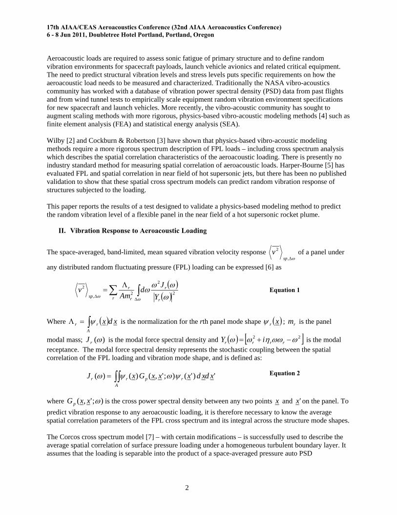
All surface FPL measurements exhibited some degree of skewness and non-normality, as summarized by the probability density function (PDF) and statistics shown in Figure 4 below. This is common when measuring high FPL levels over 165 dB (re: 2e-5 Pa) and is attributed to the onset of non-linear acoustics, as the amplitude of negative random pressure peaks approach atmospheric pressure. However, no significant skewness is observed or measured in the random time history of panel vibration response, as shown in the acceleration PDF in Figure 4. It is assumed that the skewed random pressure loading is seen by the structure as a static pressure plus an equivalent un-skewed FPL loading. Negative pressure peak distortion (eg clipping) is expected to cause some amount of “spill over” to higher frequencies in the linear spectrum analysis discussed in the next section.

-4 -2 0 2 4 6 80

0.1

0.2

0.3

0.4

0.5

Pressure ()

Pro

ba

bili

ty D

en

sity

Fu

nct

ion

PDF for Aft panel fwd

Mean = -0.00Std = 0.90Skew = 0.48Kurt = 3.52Min = -3.50 sigmaMax = 7.04 sigma

PDFGuassian

-300 -200 -100 0 100 200 3000

1

2

3

4

5

6

7

8x 10

-3

Acceleration ()

Pro

ba

bili

ty D

en

sity

Fu

nct

ion

PDF for Upper

Mean = 0.20Std = 56.62Skew = -0.01Kurt = 3.02Min = -4.69 sigmaMax = 4.34 sigma

PDFGuassian

Figure 4 Probability density functions for the random time history of surface FPL at “Aft Panel Fwd” node

#3 (left) and panel vibration acceleration response at “Upper” node #106 (right).

V. Spectrum and Spatial Correlation

The time-averaged, auto power spectral density (PSD) for a typical surface FPL measurement point and for a typical panel vibration response point is shown in Figure 5 below.

Figure 5 Surface pressure PSD in near field of plume; typical point downstream of flexible plate (left) and

typical panel vibration response PSD (right)


7

The presence of only a single apparent “peak” in the FPL spectrum suggests a single dominant jet noise generation mechanism. For a hot supersonic jet, this is most likely to be Mach wave radiation. The

PIAAV plume has an Oertel convective Mach number 25.10 aaaUM jjjIco which Greska

and Krothapalli [1] claim as a necessary condition for fully-developed Mach wave radiation. Here Uj is the jet velocity; aj is the speed of sound in the hot plume gas and a0 is the ambient speed of sound. The maximum one-third octave FPL is also observed to occur in the predicted Strouhal number range

3.02.0 St for Mach wave radiation. For the PIAAV nozzle exit diameter De and plume velocity Uj , the corresponding frequency is 2,000 – 3,000 hz. However, the measured FPL spectrum exceeds Greska and Krothapalli’s normalized pressure spectrum for Mach wave radiation, as shown in Figure 6 below.

Normalized spectrum forMach Wave radiationGreska & Krothapalli [1]

Normalized spectrum forMach Wave radiationGreska & Krothapalli [1]

M0 = 1.23

M0 = 1.05

M0 = 0.84

M0 = 0.59

M0 = 0.42

M0 = 0.27

M0 = 0.14

Mach No. HydrodynamicNear Field M0 = 1.23

M0 = 1.05

M0 = 0.84

M0 = 0.59

M0 = 0.42

M0 = 0.27

M0 = 0.14

Mach No. HydrodynamicNear Field

Figure 6 One third octave spectrum of surface pressure with normalized Mach Wave radiation spectrum [1]

overlaid (left); hydrodynamic near field pressure spectra measured by Harper-Bourne [5] at various jet Mach numbers.

One possible explanation is that the PIAAV test also measured the hydrodynamic near field pressure of the plume, as observed by Harper-Bourne [5]. However, even Harper-Bourne’s measurements – shown in Figure 6 (right) - seem to indicate that the Mach wave radiation pressure spectrum exceeds hydrodynamic near field for higher Mach number jets that are not very close to the jet shear layer. It seems more likely that Greska and Krothapalli’s normalized spectrum is only applicable to ideally-expanded, laboratory scale heated plumes; as they also found that FPL measurements on a full scale rocket plume exhibited higher spectrum levels either side of 3.02.0 St . Plume FPL Convection Velocity The apparent FPL convection velocity cU was computed from the phase gradient dfd observed in the

phase of the cross spectrum between streamwise-oriented pairs of surface FPL measurements.

1

2

df

dUc

Equation 4

where is the separation distance between the two pressure sample points used to calculate the cross spectrum.


8

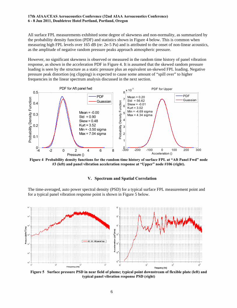
Apparent convection velocities measured in this way were high, corresponding to approximately seventy-five percent of the jet velocity. This is consistent with expected the convection velocity of large scale structures in the jet mixing layer, which are responsible for Mach wave radiation.

0 500 1000 1500 2000 2500 3000 3500 4000 4500 5000-8.5

-8

-7.5

-7

-6.5

-6

-5.5

Frequency (Hz)

Pha

se b

etw

een

Sen

s 12

and

Sen

s 13

Uc from time delay = 7281.7778 ft/s

0 500 1000 1500 2000 2500 3000 3500 4000 4500 5000-8.5

-8

-7.5

-7

-6.5

-6

-5.5

Frequency (Hz)

Pha

se b

etw

een

Sen

s 12

and

Sen

s 13


Uc = 5891 ft/s (1796 m/s)

0 500 1000 1500 2000 2500 3000 3500 4000 4500 5000-8.5

-8

-7.5

-7

-6.5

-6

-5.5

Frequency (Hz)

Pha

se b

etw

een

Sen

s 12

and

Sen

s 13


0 500 1000 1500 2000 2500 3000 3500 4000 4500 5000-8.5

-8

-7.5

-7

-6.5

-6

-5.5

Frequency (Hz)

Pha

se b

etw

een

Sen

s 12

and

Sen

s 13


Uc = 5891 ft/s (1796 m/s)

Figure 7 Observed phase gradient between two closely-spaced, streamwise orient surface pressure

transducers, used to calculate plume FPL convection velocity Plume FPL Spatial Coherence Decay The streamwise coherence decay coefficient cx, and cross flow coherence decay coefficient cy were estimated by curve-fitting to the coherence measured between respective pairs of surface pressure sensors.

101

102

103

10-2

10-1

100

Freqeuency (Hz)

Coh

eren

ce

p

Actual CoherenceCurve Fit Coherence

101

102

103

10-2

10-1

100

Freqeuency (Hz)

Coh

eren

ce

p


101

102

103

10-2

10-1

100

Freqeuency (Hz)

Coh

eren

ce

p


101

102

103

10-2

10-1

100

Freqeuency (Hz)

Coh

eren

ce

p


102

103

10-2

10-1

100

Freqeuency (Hz)

Coh

eren

ce

p


102

103

10-2

10-1

100

Freqeuency (Hz)

Coh

eren

ce

p


102

103

10-2

10-1

100

Freqeuency (Hz)

Coh

eren

ce

p


102

103

10-2

10-1

100

Freqeuency (Hz)

Coh

eren

ce

p


Figure 8 Measured coherence of surface FPL with Corcos spatial coherence decay model overlaid;

streamwise coherence (left) and cross flow coherence (right) A summary of the estimates for the three Corcos spatial correlation parameters - averaged across all sensor pairs - is presented in Table 2 below.

Average

Downstream

Upstream

Average

Downstream

Upstream

6604.176280.346726.84

7740.947491.367427.47

5467.405069.316026.22

38-41s30-33s22-25s

Uc (ft/s)

6604.176280.346726.84

7740.947491.367427.47

5467.405069.316026.22

38-41s30-33s22-25s

Uc (ft/s)

0.6440.5760.556

0.6460.6130.606

0.6430.5390.506

38-41s30-33s22-25s

Cx

0.6440.5760.556

0.6460.6130.606

0.6430.5390.506

38-41s30-33s22-25s

Cx

0.5070.5060.481

0.6600.6760.566

0.3540.3350.396

38-41s30-33s22-25s

Cy

0.5070.5060.481

0.6600.6760.566

0.3540.3350.396

38-41s30-33s22-25s

Cy

Table 2 Summary of spatial correlation parameters extracted from the cross spectrum data


9

Acoustic Reflection Time-based cross correlation measurements 2,1R were used to check the convection velocity estimates

obtained from cross spectrum phase, as described above. It was noticed that the correlation between cross-flow (y direction) sensor pairs 2,1 yyR consistently showed two correlation peaks. The strongest

correlation was at 0 corresponding to the expected 0yk nature of turbulence; with a lower but

consistent correlation peak at 0cy corresponding to acoustic propagation across the panel. There

was no evidence of similar acoustic propagation in the streamwise correlation 2,1 xxR measurements.

-1 -0.8 -0.6 -0.4 -0.2 0 0.2 0.4 0.6 0.8 1

x 10-3

-5

0

5

10x 10

4

Time (s)

Cro

ss-C

orr

Bet

wee

n S

ens

3 an

d S

ens

4

Δy3,4 = 6 inch

τ

Cro

ss-c

orre

latio

n R

3,4

(τ)

-1 -0.8 -0.6 -0.4 -0.2 0 0.2 0.4 0.6 0.8 1

x 10-3

-5

0

5

10x 10

4

Time (s)

Cro

ss-C

orr

Bet

wee

n S

ens

3 an

d S

ens

4

Δy3,4 = 6 inch

τ

Cro

ss-c

orre

latio

n R

3,4

(τ)

Plume

Plate

Nozzle

Direct field(hydrodynamic)

PIAAVPanel

Reflection(acoustic)

Plume

Plate

Nozzle

Direct field(hydrodynamic)

PIAAVPanel

Reflection(acoustic)

Figure 9 Cross-correlation between pressure sensors 3 and 4 showing second peak at delay representative of

acoustic propagation (left) and sketch illustrating path of acoustic reflections (right) On further examination, it was deduced that the PIAAV panel pressure sensors were picking up acoustic propagation from the plume - reflected from a steel plate mounted under the plume – in addition to the direct convecting hydrodynamic field of the plume. As previously identified by Bremner & Wilby [10], this mixed random pressure field needs to be represented in physics-based models with two distinct loads – acoustic and hydrodynamic – with two distinct spatial correlation descriptions. However, with insufficient pressure sensors to do wavenumber spectral filtering, one can only “guesstimate” the relative amplitudes of hydrodynamic and acoustic components. For the PIAAV SEA model, the acoustic level was set 9dB below the measured FPL (Figure 10, left) where it generated a credible panel vibration response in the SEA model, at the panel’s acoustic coincidence frequency of 5,000 Hz (Figure 10, right).

PIAAV Meas (Jet Convection)Acoustic Reflection Load (est)

SEA Acoust Reflection load (est)PIAAV Measured

Figure 10 Relative spectrum amplitude assumed for combined TBL (Corcos) and acoustic source applied to

the SEA model (left) and SEA predict vibration response to acoustic loading estimate only (right)


10

VI. Panel Damping

Assuming panel random vibration is dominated by resonant response, it is also necessary to estimate the frequency band-averaged damping for the flexible test panel bolted into the PIAAV test frame. The authors carried out several independent tests to estimate panel damping. Before and after the SRM firing, a vibration modal analysis of the panel was conducted. As part of the modal test, damping loss factor for the fundamental modes of the panel were obtained by curve-fitting the measured mobility transfer functions, under controlled impact excitation. Modal damping loss factors of one to six percent were measured in the frequency range 60 – 150 Hz as shown in Figure 11. For higher frequency damping estimates, the panel impact response data was further processed to obtain the T60 decay times in one third octave frequency bands. As is often observed at mid- to high frequencies, the T60 decay did not exhibit a uniform log-log decay rate. This is believed to be due to a significant distribution of damping levels for different modes in the analysis band. Highly damped modes decay quickly, leaving the T60 decay dominated by lightly damped modes. High frequency T60 damping loss factor estimates were therefore made at the two bounding limits – “High” damping (high decay rate) and “Low” damping (low decay rate) with a considerable range between them as shown in Figure 11. There was concern that the damping measured during these low level, controlled impact tests might underestimate non-linear effects when the panel is excited by much higher levels of excitation from plume FPL. Several methods of analyzing the panel vibration response data during the rocket motor firing were used to better estimate the panel damping. An approximate method involved curve fitting discrete mode resonance response observed in the transfer function between a panel accelerometer and the nearest surface pressure transducer. This was only possible at low frequencies but gave some indication that damping during the rocket firing test could be higher than modal test estimates. Using a more rigorous maximum entropy parametric estimation process [to be described more fully in a future technical publication] the band-averaged modal damping loss factors were found to be close to the upper bound T60 decay measurements as shown in Figure 11, below.

0%

1%

10%

10 100 1000 10000Frequency (Hz)

Da

mp

ing

Lo

ss F

act

or

TF Curve Fit

Modal Test

T60 High

T60 Low

MESAM 22-25 Seconds

MESAM 40-43 Seconds

Figure 11 Panel damping loss factor estimates using four different methods – Modal test; Transfer function

curvefit; T60 decay time and Maximum Entropy parametric estimation (MESAM)


11

VII. SEA Prediction of Panel Vibration

The foregoing analysis of the PIAAV test data yielded all of the unknown parameters required to use Statistical Energy Analysis (SEA) to predict the panel vibration response. Those unknowns are the FPL space-averaged auto PSD level, the spatial correlation parameters for a Corcos model of the FPL cross spectral properties and the damping loss factor for the panel vibration modes. Inserting those quantities into an SEA model which will solve the equivalent of Equation 1 yields a prediction of panel vibration response – in one third octave frequency bands – which is in good agreement with the measured, space-averaged panel vibration response as shown in Figure 12, below. This is a satisfactory result, demonstrating the validity of SEA methods for defining broadband random vibration environments for sensitive payloads of space flight vehicles.

SEA Est non-lin DLF + A coustic loadPIA A V MeasuredSEA Corcos + Acoustic (59 gRMS)PIAAV Measured (55 gRMS)

SEA Est non-lin DLF + A coustic loadPIA A V MeasuredSEA Corcos + Acoustic (59 gRMS)PIAAV Measured (55 gRMS)

Frequency (Hz)

Figure 12 One third octave panel vibration response; comparing statistical energy analysis (SEA) prediction

versus measured vibration on PIAAV test panel Sensitivity to Spatial Correlation The SEA model was used to assess the sensitivity of random vibration response predictions to the type of spatial correlation assumed for the measured surface FPL auto spectrum. While the PIAAV test has gone to some length to demonstrate that the near field of a SRM plume presents a convecting turbulence loading; without the cross-spectrum measurements described Section V, the vibro-acoustic analyst can only guess at the correct spatial correlation. For example, it is common to simply assume that the aeroacoustic FPL spectrum can be applied as a diffuse acoustic field [4]. Another option would be to assume a propagating random pressure field – perhaps propagating with the plume convection velocity and high coherence decay streamwise, and propagating at acoustic wave speed with low coherence decay in the cross flow direction. However, using these alternate spatial correlation models – with the same measured PIAAV surface pressure spectrum – lead to significantly different vibration response predictions in the SEA model, as shown in Figure 13. One third octave level predictions are up to 10dB higher that the measured vibration response and the overall RMS predictions over-estimate the measured RMS by 250- 300 percent.


12

SEA Propagating Wavefield (161 gRMS)PIAAV Measured (55 gRMS) SEA Diffuse Acoustic Field (128 gRMS)

Figure 13 SEA model predictions for alternative spatial correlation assumptions compared to PIAAV

measured vibration level

VIII. FEA Prediction of Panel Vibration

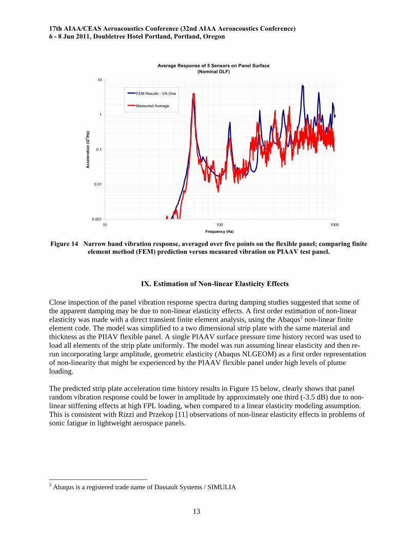
At lower frequencies – around the fundamental resonance frequency of the flexible panel – the foregoing SEA model only has a statistical estimate of the panel modal properties. But high fidelity estimates of vibration and stress response at these discrete resonances is required for sonic fatigue assessment purposes. In which case, the vibro-acoustics community typically uses a deterministic finite element model (FEM) for the flexible panel. The modal force spectral density in Equation 1 is integrated across a numerical estimate of the panel fundamental mode shapes and an estimate of the FPL cross spectrum matrix on the panel surface grid. The same Corcos model used for the SEA model was applied to a simple FEM of the structure and the averaged narrow band acceleration results are compared in Figure 14. The results show that the frequencies and amplitudes of the first two modes are captured correctly. At higher frequencies, the FEM-predicted resonant peaks begin to diverge from the measured data, most likely due to limitations in the modeling of panel boundary conditions and other uncertainties in the model. However, as has been demonstrated in Section VII, the PSD response averaged over one third octave bands is still predicted to sufficient accuracy. These results indicate that the Corcos model, using measured parameters such as convection velocity, is proven satisfactory (at least to first order) for predicting low frequency narrow band response as well as the mid to high frequency band-averaged response.


13

Average Response of 5 Sensors on Panel Surface(Nominal DLF)

0.001

0.01

0.1

1

10

10 100 1000

Frequency (Hz)

Acc

eler

atio

n (

G2/H

z)

FEM Results - VA-One

Measured Average

Figure 14 Narrow band vibration response, averaged over five points on the flexible panel; comparing finite

element method (FEM) prediction versus measured vibration on PIAAV test panel.

IX. Estimation of Non-linear Elasticity Effects

Close inspection of the panel vibration response spectra during damping studies suggested that some of the apparent damping may be due to non-linear elasticity effects. A first order estimation of non-linear elasticity was made with a direct transient finite element analysis, using the Abaqus2 non-linear finite element code. The model was simplified to a two dimensional strip plate with the same material and thickness as the PIIAV flexible panel. A single PIAAV surface pressure time history record was used to load all elements of the strip plate uniformly. The model was run assuming linear elasticity and then re-run incorporating large amplitude, geometric elasticity (Abaqus NLGEOM) as a first order representation of non-linearity that might be experienced by the PIAAV flexible panel under high levels of plume loading. The predicted strip plate acceleration time history results in Figure 15 below, clearly shows that panel random vibration response could be lower in amplitude by approximately one third (-3.5 dB) due to non-linear stiffening effects at high FPL loading, when compared to a linear elasticity modeling assumption. This is consistent with Rizzi and Przekop [11] observations of non-linear elasticity effects in problems of sonic fatigue in lightweight aerospace panels.

2 Abaqus is a registered trade name of Dassault Systems / SIMULIA


14

0 1.0 2.0 3.0 4.0 5.0 0 1.0 2.0 3.0 4.0 5.0 Time (sec)

G G

Time (sec)0 1.0 2.0 3.0 4.0 5.0 0 1.0 2.0 3.0 4.0 5.0 0 1.0 2.0 3.0 4.0 5.0

Time (sec)

G G

Time (sec)0 1.0 2.0 3.0 4.0 5.0

Figure 15 Acceleration time history of an “equivalent strip plate”, predicted by finite element model;

assuming linear elasticity (left) and assuming non-linear elasticity (right) The predicted strip plate acceleration PSD results in Figure 16 below, clearly shows that non-linear elasticity shifts resonance response to higher frequencies and broadens the resonance response peak. This behavior is also as observed by Rizzi and Przekop [11]. The non-linear smearing of time-averaged resonance peaks may therefore be a factor to consider in the use of parametric system identification methods for estimating “operating damping” levels, previewed in the linear vibro-acoustic analysis reported in this paper.

PS

D (

G2 /

Hz)

0 500 1000 1500 2000 2500 Frequency (Hz)

0 500 1000 1500 2000 2500 Frequency (Hz)

PS

D (

G2 /

Hz)

PS

D (

G2 /

Hz)

0 500 1000 1500 2000 2500 Frequency (Hz)

0 500 1000 1500 2000 2500 Frequency (Hz)

PS

D (

G2 /

Hz)

Figure 16 Acceleration PSD of an “equivalent strip plate”, predicted by finite element model; assuming linear elasticity (left) and assuming non-linear elasticity (right)


15

X. Conclusions

The use of a Corcos model for plume loading in both the statistical energy analysis (SEA) validation results summarized in Figure 12, and the finite element analysis results summarized in Figure 14, are satisfactory for the purpose of defining random vibration environment for spacecraft and launch vehicles. These results show that physics-based modeling is a valid alternative to empirical scaling methods traditionally used in the NASA vibroacoustic community. However, this paper also highlights that physics-based vibro-acoustic modeling requires estimation of the spatial cross-spectral characteristics of an aeroacoustic FPL load. While it is NASA standard practice to measure the space-averaged auto PSD for aeroacoustic loads, this paper has shown how and why it is also necessary to measure the corresponding spatial correlation parameters of the aeroacoustic FPL load.

XI. Acknowledgments

The authors acknowledge the NASA Engineering Safely Center funding for this work and thank NASA Marshall Space Flight Center for making the horizontal rocket firing test facility available for the PIAAV test. Special thanks to Mike Nucci at ATA Engineering, who conducted the non-linear finite element analysis.

XII. References

[1] Greska, B., Krothapalli, A., Horne, W.C. and Burnside, N., “A Near-Field Study of High Temperature Supersonic Jets,” AIAA 2008-3026 Proc. AIAA Aeroacoustics Conf. , Vancouver BC, 2008

[2] Wilby, J.F., “The Response of Simple Panels to Turbulent Boundary Layer Excitation.” Air Force Flight Dynamics Laboratory. AFFDL-TR-67-70, October 1967

[3] Cockburn, J.A., Robertson, J.E., “Vibration Response of Spacecraft Shrouds to In-Flight Fluctuating Pressures,” Journal of Sound & Vibration, Vol. 33, No. 4, April, 1974

[4] Himelblau, H., Kern, D.L., et al (Eds.) Dynamic Environmental Criteria, NASA Technical Handbook NASA-HDBK-7005, March 2001

[5] Harper-Bourne, M. “On Modeling the Hydrodynamic Field of High Speed Jets”, AIAA 2004-2830, Proc. 10th AIAA/CEAS Aeroacoustics Conf., 2004

[6] Bremner, P.G. “Finite Element Based Vibro-Acoustics of Panel Systems”, Proc. 5th Intnl. Conf. on Finite Element Methods in Engineering, Melbourne, August 1987

[7] Corcos G.M., “The structure of the turbulent pressure field in boundary-layer flows,” Journal of Fluid Mechanics, Vol. 18, No. 3, March, 1964

[8] Osteholt, D. and Knox, D, . “Measuring Fluctuating Pressure Levels and Vibration Response in a Jet Plume”, Proc. 26th Aerospace Testing Seminar, Los Angeles, 2010.

[9] Krothapalli, A, Arakeri V. and Greska, B., “Identifying Mach Wave Radiation: A Review and an Extension” AIAA 2003-1200, 41st AIAA Aerosciences Meeting, Reno NV, 2003.

[10] Bremner P.G. & Wilby, J.F, “Aero-Vibro-Acoustics: Problem Statement and Model-based Design Methods,” AIAA 2002-2551, Proc. AIAA Aeroacoustics Conf., Breckenridge CO , 2002

[11] Rizzi, S.A. & Przekop, A. “Estimation of Sonic Fatigue by Reduced-Order Finite Element Based Analyses” Proc. IX Intnl. Conf. on Recent Advances in Structural Dynamics, Southampton, UK, July 2006

validation of methods to predict vibration of a panel in the … · · 2013-04-1017th aiaa/ceas...

Documents