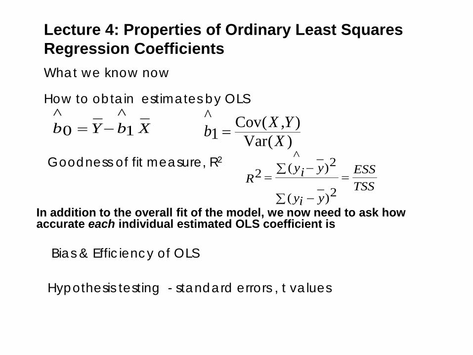
How to obtain estimates by OLS

Goodness of fit measure, R2

Bias & Efficiency of OLS

Hypothesis testing - standard errors , t values

Lecture 4: Properties of Ordinary Least Squares Regression Coefficients What we know now

_1

^_0

^XbYb −=

)(Var),(Cov

1^

XYXb =

In addition to the overall fit of the model, we now need to ask how accurate each individual estimated OLS coefficient is

TSSESS

yiy

yiyR =

∑ −

∑ −=

2)_

(

2)_^

(2

To do this need to make some assumptions about the behaviour of the (true) residual term that underlies our view of the world

Based on a set of beliefs called the Gauss-Markov

assumptions → Gauss-Markov Theorem which underpins the usefulness of OLS as an estimation technique Why make assumptions about the residuals and not the betas? - The behaviour/ properties of the betas are derived from the assumptions we make about the residuals

Gauss-Markov Theorem (attributed to Carl-Friedrich Gauss, 1777 – 1855 & Andrey Markov 1856-1922 )

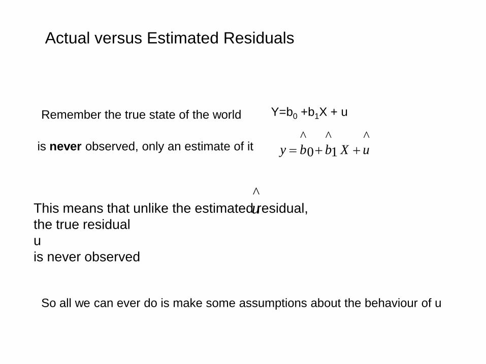
^uThis means that unlike the estimated residual,

the true residual u is never observed

So all we can ever do is make some assumptions about the behaviour of u

Remember the true state of the world Y=b0 +b1X + u

is never observed, only an estimate of it ^

1^

0^

uXbby ++=

Actual versus Estimated Residuals

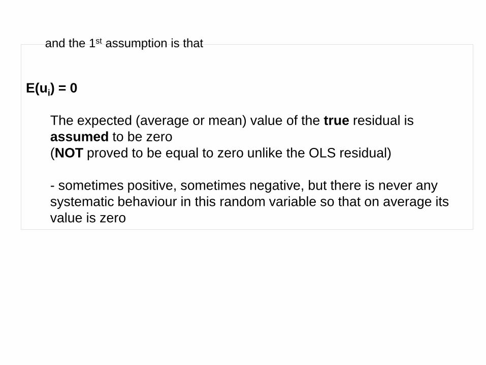
E(ui) = 0

The expected (average or mean) value of the true residual is assumed to be zero (NOT proved to be equal to zero unlike the OLS residual) - sometimes positive, sometimes negative, but there is never any systematic behaviour in this random variable so that on average its value is zero

and the 1st assumption is that

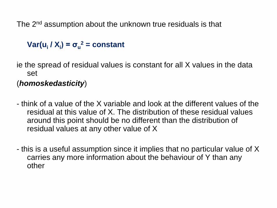
The 2nd assumption about the unknown true residuals is that Var(ui / Xi) = σu

2 = constant ie the spread of residual values is constant for all X values in the data

set (homoskedasticity)

- think of a value of the X variable and look at the different values of the

residual at this value of X. The distribution of these residual values around this point should be no different than the distribution of residual values at any other value of X

- this is a useful assumption since it implies that no particular value of X

carries any more information about the behaviour of Y than any other

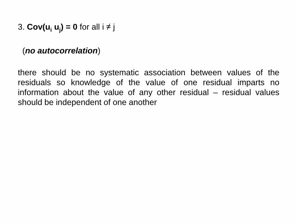
3. Cov(ui uj) = 0 for all i ≠ j (no autocorrelation) there should be no systematic association between values of the residuals so knowledge of the value of one residual imparts no information about the value of any other residual – residual values should be independent of one another

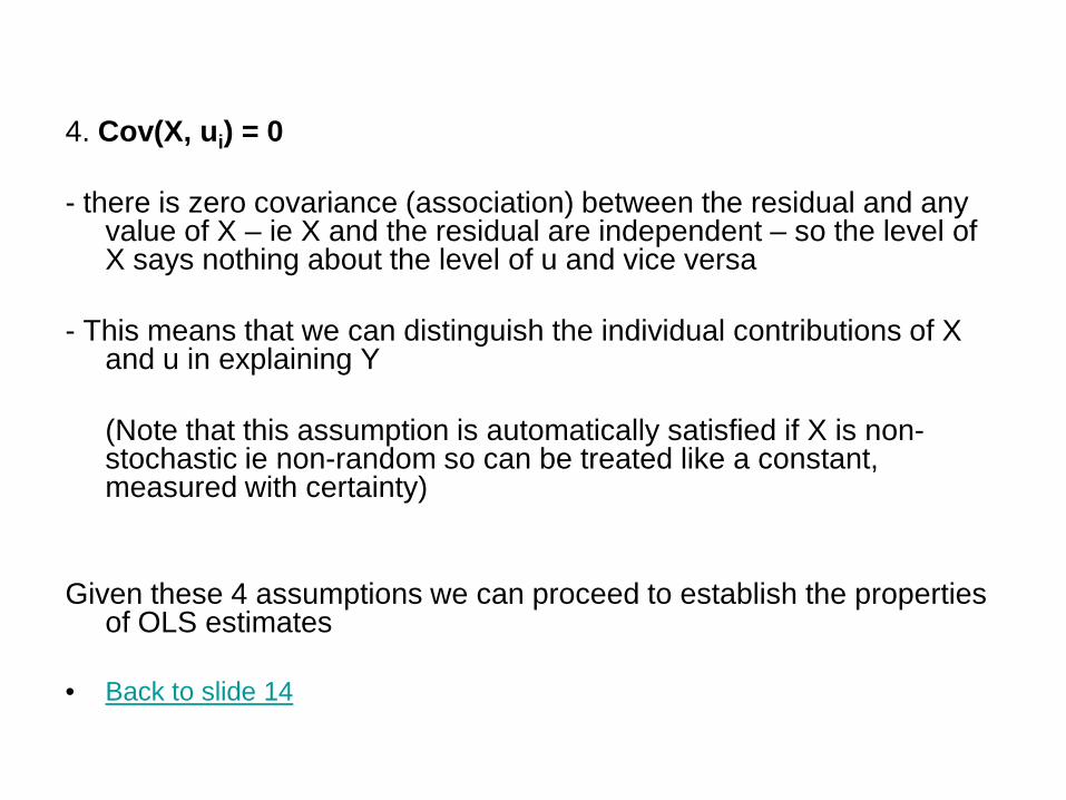
4. Cov(X, ui) = 0

- there is zero covariance (association) between the residual and any value of X – ie X and the residual are independent – so the level of X says nothing about the level of u and vice versa

- This means that we can distinguish the individual contributions of X

and u in explaining Y (Note that this assumption is automatically satisfied if X is non-

stochastic ie non-random so can be treated like a constant, measured with certainty)

Given these 4 assumptions we can proceed to establish the properties

of OLS estimates • Back to slide 14

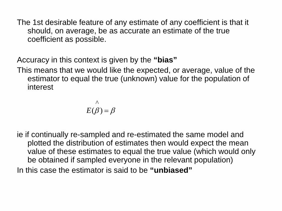
The 1st desirable feature of any estimate of any coefficient is that it should, on average, be as accurate an estimate of the true coefficient as possible.

Accuracy in this context is given by the “bias” This means that we would like the expected, or average, value of the

estimator to equal the true (unknown) value for the population of interest

ie if continually re-sampled and re-estimated the same model and plotted the distribution of estimates then would expect the mean value of these estimates to equal the true value (which would only be obtained if sampled everyone in the relevant population)

In this case the estimator is said to be “unbiased”

ββ =)(^

E

Are OLS estimates biased?

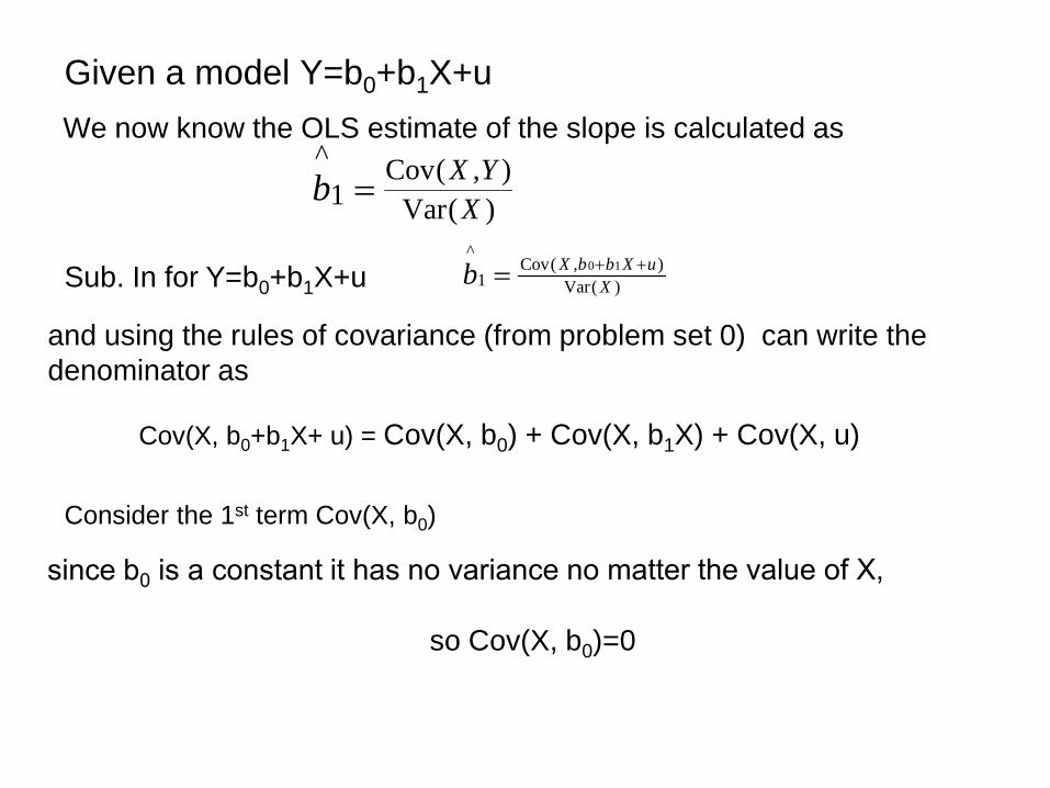
Given a model Y=b0+b1X+u We now know the OLS estimate of the slope is calculated as

)(Var),(Cov

1^

XYXb =

and using the rules of covariance (from problem set 0) can write the denominator as

Cov(X, b0+b1X+ u) = Cov(X, b0) + Cov(X, b1X) + Cov(X, u)

so Cov(X, b0)=0

Sub. In for Y=b0+b1X+u

Consider the 1st term Cov(X, b0)

)(Var),(Cov

1

^10

XuXbbXb ++=

– since b1 is a constant can take it outside the bracket

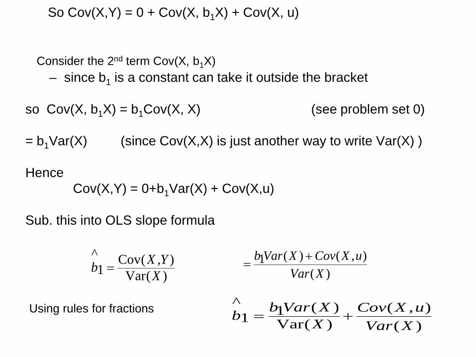
so Cov(X, b1X) = b1Cov(X, X) (see problem set 0) = b1Var(X) (since Cov(X,X) is just another way to write Var(X) ) Hence Cov(X,Y) = 0+b1Var(X) + Cov(X,u) Sub. this into OLS slope formula

)(Var),(Cov

1^

XYXb =

)(),(

)(Var)(11

^

XVaruXCov

XXVarbb +=

So Cov(X,Y) = 0 + Cov(X, b1X) + Cov(X, u)

Consider the 2nd term Cov(X, b1X)

)(),()(1

XVaruXCovXVarb +

=

Using rules for fractions

)(),(

)(Var)(

1^

1

XVaruXCovb X

XVarb +=

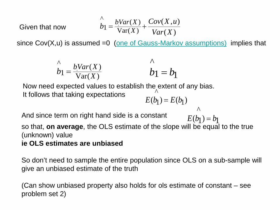
since Cov(X,u) is assumed =0 (one of Gauss-Markov assumptions) implies that

)(Var)(

1^

1

XXVarbb =

Now need expected values to establish the extent of any bias. It follows that taking expectations

)()( 1^1 bEbE =

so that, on average, the OLS estimate of the slope will be equal to the true (unknown) value ie OLS estimates are unbiased So don’t need to sample the entire population since OLS on a sub-sample will give an unbiased estimate of the truth (Can show unbiased property also holds for ols estimate of constant – see problem set 2)

11^

bb =

1)^1( bbE =

Given that now

And since term on right hand side is a constant

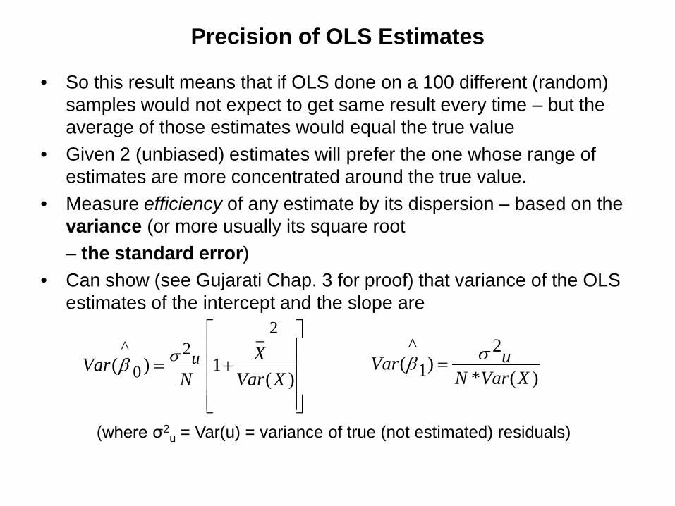
Precision of OLS Estimates

• So this result means that if OLS done on a 100 different (random) samples would not expect to get same result every time – but the average of those estimates would equal the true value

• Given 2 (unbiased) estimates will prefer the one whose range of estimates are more concentrated around the true value.

• Measure efficiency of any estimate by its dispersion – based on the variance (or more usually its square root

– the standard error) • Can show (see Gujarati Chap. 3 for proof) that variance of the OLS

estimates of the intercept and the slope are

+=)(

1)(

2_2

0^

XVarX

NVar uσβ

)(*

2)1

^(

XVarNuVar σβ =

(where σ2u = Var(u) = variance of true (not estimated) residuals)

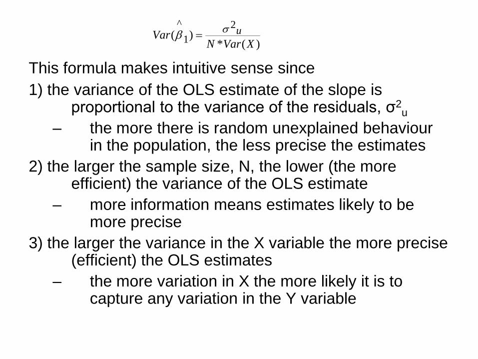
This formula makes intuitive sense since 1) the variance of the OLS estimate of the slope is

proportional to the variance of the residuals, σ2u

– the more there is random unexplained behaviour in the population, the less precise the estimates

2) the larger the sample size, N, the lower (the more efficient) the variance of the OLS estimate

– more information means estimates likely to be more precise

3) the larger the variance in the X variable the more precise (efficient) the OLS estimates

– the more variation in X the more likely it is to capture any variation in the Y variable

)(*)(

21

^

XVarNVar uσβ =

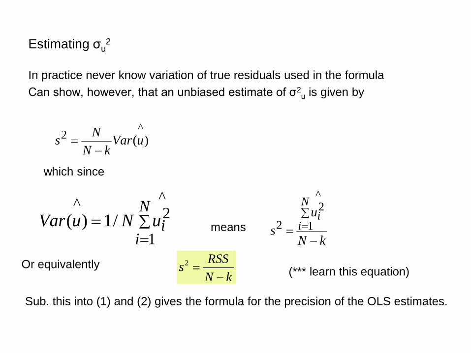
Estimating σu2

In practice never know variation of true residuals used in the formula Can show, however, that an unbiased estimate of σ2

u is given by

kN

us

N

ii

−=

∑=1

^2

2

)(^2 uVar

kNNs−

=

Sub. this into (1) and (2) gives the formula for the precision of the OLS estimates.

∑=

=N

iiuNuVar

1

^2^

/1)(

which since

means

kNRSSs−

=2(*** learn this equation) Or equivalently

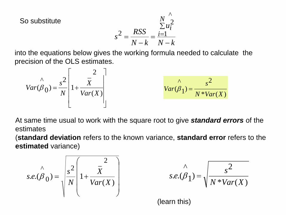
into the equations below gives the working formula needed to calculate the precision of the OLS estimates.

At same time usual to work with the square root to give standard errors of the estimates (standard deviation refers to the known variance, standard error refers to the estimated variance)

+=)(

1).(.

2_20

^

XVarX

Nses β

)(*

2)1

^.(.

XVarNses =β

+=)(

2_

12

)0^

(XVar

XNsVar β

kN

u

kNRSSs

N

ii

−=

−=

∑=1

^2

2

So substitute

)(*

2)1

^(

XVarNs

Var =β

(learn this)

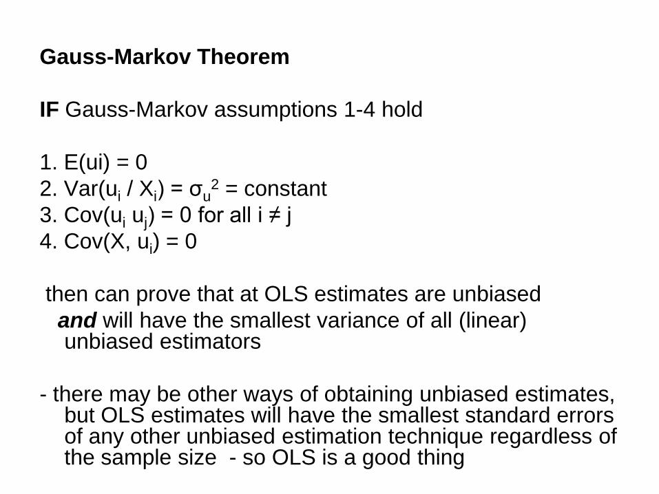
Gauss-Markov Theorem IF Gauss-Markov assumptions 1-4 hold 1. E(ui) = 0 2. Var(ui / Xi) = σu

2 = constant 3. Cov(ui uj) = 0 for all i ≠ j 4. Cov(X, ui) = 0 then can prove that at OLS estimates are unbiased and will have the smallest variance of all (linear)

unbiased estimators - there may be other ways of obtaining unbiased estimates,

but OLS estimates will have the smallest standard errors of any other unbiased estimation technique regardless of the sample size - so OLS is a good thing

Hypothesis Testing Now know how to estimate and interpret OLS regression coefficients We know also that OLS gives us unbiased and efficient (smallest variance) estimates But just because a variable has a large coefficient does not necessarily mean its contribution to the model is significant. This means we need to understand the ideas behind standard errors, the t value and how to use t values in applied work

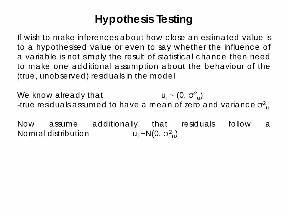
Hypothesis Testing If wish to make inferences about how close an estimated value is to a hypothesised value or even to say whether the influence of a variable is not simply the result of statistical chance then need to make one additional assumption about the behaviour of the (true, unobserved) residuals in the model We know already that ui ~ (0, σ2

u) -true residuals assumed to have a mean of zero and variance σ2

u Now assume additionally that residuals follow a Normal distribution ui ~N(0, σ2

u)

Now assume additionally that residuals follow a Normal distribution ui ~N(0, σ2

u) (Since residuals capture influence of many unobserved (random)

variables, can use Central Limit Theorem which says that the sum of a set of random variables will have a normal distribution)

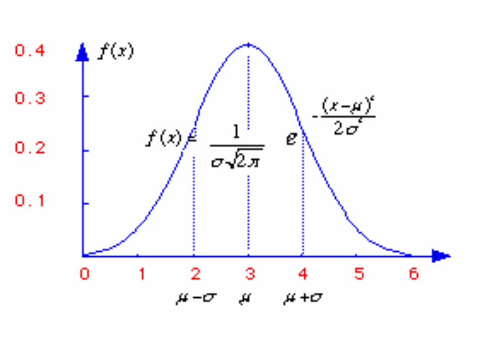
If a variable is normally distributed we know that it is Symmetric centred on its mean and that: 66% of values lie within mean 1*standard deviation 95% of values lie within mean 1.96*standard dev. 99% of values lie within mean 2.9*standard dev.

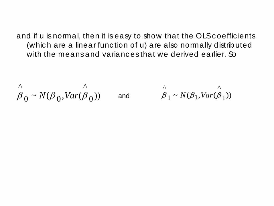
and if u is normal, then it is easy to show that the OLS coefficients

(which are a linear function of u) are also normally distributed with the means and variances that we derived earlier. So

))(,(~ 0^

00^

βββ VarN and ))(,(~ 1^

11^

βββ VarN

→ Gauss-Markov Theorem which underpins the usefulness of OLS as an estimation technique (attributed to Carl-Friedrich Gauss, 1777 – 1855 & Andrey Markov 1856-1922 )